Embed Size (px)
Citation preview

Navier-Stokes Equations with Degenerate
Viscosity, Vacuum and Gravitational Force
Renjun Duan
Department of Mathematics, City University of Hong Kong83 Tat Chee Avenue, Kowloon, Hong Kong, P.R. China
Email: renjun [email protected]
Tong Yang
Liu Bie Ju Centre of Mathematics, City University of Hong Kong83 Tat Chee Avenue, Kowloon, Hong Kong, P.R. China
Email: [email protected]
Changjiang Zhu
Laboratory of Nonlinear Analysis, Department of MathematicsCentral China Normal University, Wuhan 430079, P.R. China
Email: [email protected]
Abstract
The global existence of weak solutions to the compressible Navier-Stokes equationswith vacuum attracts many research interests recently. For the isentropic gas, theviscosity coefficient depends on density function from physical point of view. Whenthe density function connects to vacuum continuously, the vacuum degeneracy givessome analytic difficulties in proving global existence. In this paper, we consider thiscase with gravitational force and fixed boundary condition. By giving a series of apriori estimates on the solution coping with the degeneracy of vacuum, gravitationalforce and boundary effect, we give global existence and uniqueness results similar tothe case without force and boundary.
Key words: Navier-Stokes equations, vacuum, a priori estimates, global existence.
1. Introduction
Consider the one-dimensional compressible Navier-Stokes equations for isentropic flowwith gravitational force in Eulerian coordinates: ρτ + (ρu)ξ = 0,
(ρu)τ + (ρu2 + P (ρ))ξ = (µuξ)ξ + ρg, in y(τ) < ξ < 0, τ > 0,(1.1)
1
2 R.J. DUAN, T. YANG AND C.J. ZHU
with initial data
ρ(ξ, 0) = ρ0(ξ), u(ξ, 0) = u0(ξ), on y(0) ≤ ξ ≤ 0, (1.2)
and boundary conditionu(1, τ) = 0. (1.3)
Here the unknown functions ρ = ρ(ξ, τ) and u = u(ξ, τ) represent the density and velocityrespectively. P (ρ) = Aργ is the pressure with A being a positive constant and γ > 1,µ ≥ 0 is the viscosity coefficient, and g > 0 is the gravitational constant. y(τ) is thevacuum boundary, i.e., the particle path separating the gas and the vacuum, satisfying
dy
dτ= u(y(τ), τ), ρ(y(τ), τ) = 0. (1.4)
Our main concern here is the global existence and the uniqueness of weak solutionswith some regularity for the description on the vacuum boundary to the above initialboundary value problem when the viscosity coefficient depends on the density function. Itis a continuation of works in [26, 28, 29, 30] which are about the case when no boundary andexternal force are considered. As usual, the main estimate is to obtain the lower boundon the density function. When the gas connects to vacuum continuously, the viscositycoefficient also vanishes at the boundary. In this case, we can expect only a lower boundof the density function in the form of a power function xβ for some constant β determinedby the initial data and viscosity coefficient.
Furthermore, the interface separating the gas and vacuum propagates with finite speedbecause of the hyperbolic-parabolic property of the system (1.1). And the proof of thisfinite speed propagation follows from the lower bound of the density function estimate.
Some of the previous works in this direction can be summarized as follows. Whenthe viscosity coefficient µ is a constant, there is no continuous dependence on the initialdata to the Navier-Stokes equations (1.1) with vacuum, see [8]. This leads to the studyon the initial boundary value problem instead of initial value problem. For this, the freeboundary problem of one dimensional Navier-Stokes equations with one boundary fixedand the other connected to vacuum was investigated in [19], where the global existence ofthe weak solutions was proved. Similar results were obtained in [20] for the equations ofspherically symmetric motion of viscous gases. Furthermore, the free boundary problemof the one-dimensional viscous gas expanding into the vacuum has been studied by manypeople, see [19, 20, 25] and reference therein. A further understanding of the regularityand behavior of solutions near the interfaces between the gas and vacuum was given in[15].
It is known that the physically important case related to vacuum is when µ is not aconstant, see [23, 24, 31]. It can be seen from the derivation of the Navier-Stokes equationsfrom the Boltzmann equation through the Chapman-Enskog expansion to the second order,cf. [5], where the viscosity coefficient depends on the temperature. For isentropic flow,this dependence is reduced to the dependence on the density by the laws of Boyle andGay-Lussac for ideal gas as discussed in [14]. When the viscosity coefficient is a function
Navier-Stokes Equations with Vacuum 3
of density, such as µ = cρθ with c and θ being positive constants, the local existence ofweak solutions to Navier-Stokes equations with vacuum was studied in [14] on the casewhen the initial density connects to vacuum with discontinuities. The global existence ofweak solutions was obtained in [21] with the same assumption when 0 < θ < 1
3 and it islater generalized to the cases for 0 < θ < 1
2 and 0 < θ < 1 in [28] and [11] respectively.It is noticed that the above analysis is based on the uniform positive lower bound of
the density with respect to the construction of the approximate solutions. This estimate iscrucial because the other estimates for the convergence of a subsequence of the approximatesolutions and the uniqueness of the solution thus obtained will follow from the estimationby standard techniques as long as the vacuum does not appear in the solutions in finitetime. And this uniform positive lower bound on the density function can only be obtainedwhen the density function connects to vacuum with discontinuities. In this situation, thedensity function is positive for any finite time and thus the viscosity coefficient nevervanishes. This good property of the solution was obtained and used to prove globalexistence of solutions to (1.1) when the initial data is of compact support, cf. [11, 21, 28].
If the density function connects to vacuum continuously, there is no positive lowerbound for the density function and the viscosity coefficient vanishes at vacuum. Thisdegeneracy in the viscosity coefficient gives arise to new analysis difficulties because ofthe less regularizing effect on the solutions. A local existence result was obtained on thiscase in [29], and global existence result in [30] for 0 < θ < 2
9 and in [26] for 0 < θ < 13 .
Another difficulty comes from the singularity at the vacuum boundary when the densityfunction connects to vacuum continuously. This can be seen from the analysis in [25] onthe non-global existence of regular solution to Navier-Stokes equations when the densityfunction is of compact support with the viscosity coefficient being constant. The proofthere is based on the estimation on the growth rate of the support on density function intime t. If the growth rate is sub-linear, then a nonlinear functional was introduced in [25]which yields the non-global existence of regular solutions. The intuitive explanation ofthis phenomena comes from the consideration of the pressure in the gas. No matter howsmooth the initial data is, the pressure of the gas will build up at the vacuum boundaryin finite time and it will push the gas into the vacuum region. This effect can not becompensated by the dissipation from the viscosity so that the support of the gas staysunchanged. This is different from the system of Euler-Poisson equations for gaseous starswhere the pressure and the gravitational force can become balanced to have a stationarysolutions. In the case of compressible Navier-Stokes equation, the pressure will have theeffort on the evolution of the vacuum boundary in finite time so that the density functionat the interface will not be smooth. This singularity at the derivatives , maybe of thesecond order for one-dimensional case, cf. [25], gives some analytic difficulty, but it can beovercome by introducing some appropriate weights in the energy estimates as in [30, 26, 4].Notice that these weight functions vanish at the vacuum boundary.
The last but not least, there has been a lot of investigation on the Navier-Stokesequations when the initial density is away from vacuum, both for smooth initial data ordiscontinuous initial data, and one dimensional or multidimensional problems. For these

4 R.J. DUAN, T. YANG AND C.J. ZHU
results, please refer to [6, 8, 10, 12, 13, 22] and reference therein. The non-appearanceof vacuum in the solutions for any finite time if the initial data does not contain vacuumwas proved in [9]. It is not known yet whether the corresponding result holds for thedensity-dependent viscosity.
The rest of this paper is organized as follows. In Section 2, we will give the definitionof the weak solution and then state the main theorems in this paper. In Section 3, wewill prove some a priori estimates for the global existence of weak solutions to (1.1)-(1.3).In Section 4, we will construct the approximate solutions by the line method and state aseries of lemmas following the estimates on Section 3. A uniqueness theorem for the weaksolution will be given in the last section.
2. The Main Theorems
The free boundary value problem (1.1)-(1.4) can be reformed in Lagrangian coordinatesby using the transformation:
x =∫ ξ
0ρ(z, τ)dz, t = τ, i.e.,
∂
∂τ=
∂
∂t− ρu
∂
∂x,
∂
∂ξ= ρ
∂
∂x,
Now, considering the position of boundary X(τ) = x(y(τ), τ) =∫ y(τ)0 ρ(z, τ)dz and using
(1.1)1, (1.3) and (1.4), we have dXdτ = 0, i.e., X is independent of τ . Thus we can set
X ≡∫ y(0)0 ρ(z, 0)dz. We consider y(0) > −∞ and X > −∞, i.e., a finite total mass on a
finite interval. After rescaling the variables, the problem (1.1)-(1.4) is transformed to thefollowing fixed boundary problem: ρt + ρ2ux = 0,
ut + P (ρ)x = (µρux)x + g, 0 < x < 1, t > 0,(2.1)
with the boundary conditions ρ(0, t) = 0 at the free end,
u(1, t) = 0 at the fixed end,(2.2)
the initial data(ρ, u)(x, 0) = (ρ0(x), u0(x)), 0 ≤ x ≤ 1, (2.3)
and the compatibility conditions at x = 0, 1,
ρ0(0) = 0, u0(1) = 0, (2.4)
where P (ρ) = Aργ , µ = cρθ. We normalize A = 1 and c = 1.Throughout this paper, the assumptions on the initial data, θ and γ can be stated as
follows:
(A1) 0 < θ < 13 , γ > 1;

Navier-Stokes Equations with Vacuum 5
(A2) There exists a positive constant C such that 0 ≤ ρ0(x) ≤ C with ρ0(0) = 0,ρ0(1) > 0, (ρ0(x))−1 ∈ L1([0, 1]), (ργ
0(x))x ∈ L2([0, 1]), u0(x) ∈ L∞([0, 1]) and (ρ1+θ0 (x)u0x(x))x ∈
L2([0, 1]);
(A3) For 0 < θ < 13 , there exists a sufficiently large positive integer m such that
2m− 14m2
≤ θ ≤ 4m2 − 8m+ 312m2 − 14m+ 2
. (2.5)
For such fixed positive integer m, let x2m−2[(ρθ
0)x
]2m∈ L1([0, 1]).
Under the assumptions (A1)-(A3), we will prove the existence of global weak solutionsto the initial boundary value problem (2.1)-(2.4). The weak solution defined bellow issimilar to the one in [21].
Definition 2.1. A pair of functions (ρ(x, t), u(x, t)) is called a global weak solution tothe initial boundary value problem (2.1)-(2.4), if for any T > 0
ρ, u ∈ L∞([0, 1]× [0, T ]) ∩ C1([0, T ];L2([0, 1])), (2.6)
ρ1+θux ∈ L∞([0, 1]× [0, T ]) ∩ C12 ([0, T ];L2([0, 1])). (2.7)
Furthermore, the following equations hold:∫ ∞
0
∫ 1
0(ρφt − ρ2uxφ)dxdt+
∫ 1
0ρ0(x)φ(x, 0)dx = 0, (2.8)
and ∫ ∞
0
∫ 1
0(uψt + (P (ρ)− µρux)ψx − gψ)dxdt+
∫ 1
0u0(x)ψ(x, 0)dx = 0, (2.9)
for any test functions φ(x, t) and ψ(x, t) ∈ C∞0 (Ω) with Ω = (x, t) : 0 ≤ x ≤ 1, t ≥ 0.
In what follows, we always use C (C(T )) to denote a generic positive constant depend-ing only on the initial data (or the given time T ).
We now state the main theorem in this paper as follows:
Theorem 2.2 (Existence). Under the conditions (A1)-(A3), the free boundary problem(2.1)-(2.4) has a weak solution (ρ(x, t), u(x, t)) which satisfies Definition 2.1 and ρ(x, t)satisfies
C(T )x1+k3 ≤ ρ(x, t) ≤ C(T ), (2.10)
where k3 satisfies
2mθ2m(1− θ)− 1
= max
12m− 1
,2mθ
2m(1− θ)− 1
≤ k3 ≤
12θ− 1− 1
(2m− 1)θ. (2.11)
6 R.J. DUAN, T. YANG AND C.J. ZHU
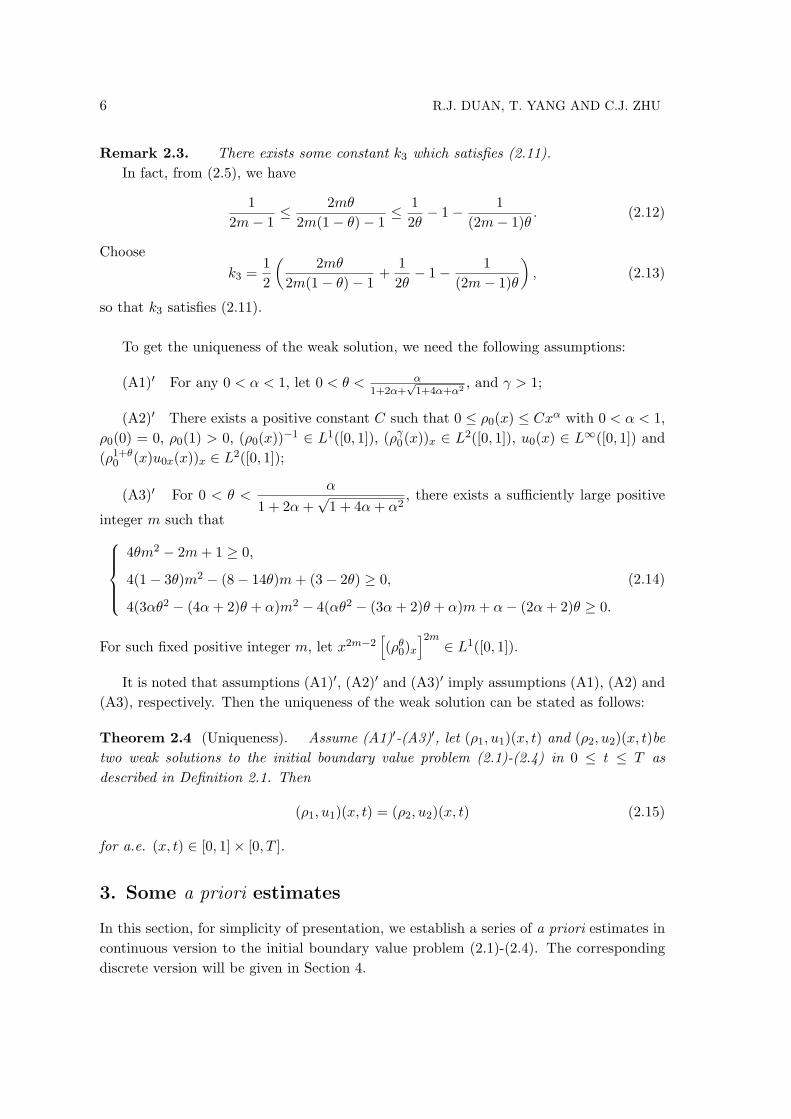
Remark 2.3. There exists some constant k3 which satisfies (2.11).In fact, from (2.5), we have
12m− 1
≤ 2mθ2m(1− θ)− 1
≤ 12θ− 1− 1
(2m− 1)θ. (2.12)
Choosek3 =
12
(2mθ
2m(1− θ)− 1+
12θ− 1− 1
(2m− 1)θ
), (2.13)
so that k3 satisfies (2.11).
To get the uniqueness of the weak solution, we need the following assumptions:
(A1)′ For any 0 < α < 1, let 0 < θ < α1+2α+
√1+4α+α2
, and γ > 1;
(A2)′ There exists a positive constant C such that 0 ≤ ρ0(x) ≤ Cxα with 0 < α < 1,ρ0(0) = 0, ρ0(1) > 0, (ρ0(x))−1 ∈ L1([0, 1]), (ργ
0(x))x ∈ L2([0, 1]), u0(x) ∈ L∞([0, 1]) and(ρ1+θ
0 (x)u0x(x))x ∈ L2([0, 1]);
(A3)′ For 0 < θ <α
1 + 2α+√
1 + 4α+ α2, there exists a sufficiently large positive
integer m such that4θm2 − 2m+ 1 ≥ 0,
4(1− 3θ)m2 − (8− 14θ)m+ (3− 2θ) ≥ 0,
4(3αθ2 − (4α+ 2)θ + α)m2 − 4(αθ2 − (3α+ 2)θ + α)m+ α− (2α+ 2)θ ≥ 0.
(2.14)
For such fixed positive integer m, let x2m−2[(ρθ
0)x
]2m∈ L1([0, 1]).
It is noted that assumptions (A1)′, (A2)′ and (A3)′ imply assumptions (A1), (A2) and(A3), respectively. Then the uniqueness of the weak solution can be stated as follows:
Theorem 2.4 (Uniqueness). Assume (A1)′-(A3)′, let (ρ1, u1)(x, t) and (ρ2, u2)(x, t)betwo weak solutions to the initial boundary value problem (2.1)-(2.4) in 0 ≤ t ≤ T asdescribed in Definition 2.1. Then
(ρ1, u1)(x, t) = (ρ2, u2)(x, t) (2.15)
for a.e. (x, t) ∈ [0, 1]× [0, T ].
3. Some a priori estimates
In this section, for simplicity of presentation, we establish a series of a priori estimates incontinuous version to the initial boundary value problem (2.1)-(2.4). The correspondingdiscrete version will be given in Section 4.

Navier-Stokes Equations with Vacuum 7
Lemma 3.1. Under the conditions of Theorem 2.2, we have that for 0 < x < 1, t > 0,
(ρθ)t(x, t) = −θρ1+θux(x, t), (3.1)
(ρ1+θux
)(x, t) = ργ(x, t) +
∫ x
0ut(y, t)dy − gx, (3.2)
and
ρθ(x, t) + θ
∫ t
0ργ(x, s)ds = ρθ
0(x) + θgxt− θ
∫ t
0
∫ x
0ut(y, s)dyds. (3.3)
Proof. From (2.1)1, we have
(ρθ)t = θρθ−1ρt = −θρ1+θux,
which implies (3.1).Integrating (2.1)2 over [0, x] and using the boundary condition (2.2), we have
∫ x
0ut(y, t)dy + ργ(x, t) =
(ρ1+θux
)(x, t) + gx,
which implies (3.2).Integrating (3.1) over [0, t], we have
ρθ(x, t) = −θ∫ t
0(ρ1+θux)(x, s)ds+ ρθ
0(x). (3.4)
From (3.2) and (3.4), we get (3.3). Lemma 3.1 is completed.
Lemma 3.2. Under the conditions of Theorem 2.2, the following energy estimateshold: ∫ 1
0
(12u2 +
1γ − 1
ργ−1 +gx
ρ
)dx+
∫ t
0
∫ 1
0ρ1+θu2
xdxdt
=∫ 1
0
(12u2
0(x) +1
γ − 1ργ−10 (x) +
gx
ρ0(x)
)dx
≤ C, 0 < t ≤ T. (3.5)
Proof. Multiplying (2.1)1 and (2.2)2 by ργ−2 − gxρ−2 and u, respectively and summingthem, we get
d
dt
(12u2 +
1γ − 1
ργ−1 +gx
ρ
)+ (ργu)x − gxux = u(ρ1+θux)x + gu. (3.6)

8 R.J. DUAN, T. YANG AND C.J. ZHU
Integrating (3.6) over [0, 1]× [0, t] and using the boundary condition (2.2) and the assump-tion (A1) and (A2), we have∫ 1
0
(12u2 +
1γ − 1
ργ−1 +gx
ρ
)dx+
∫ t
0
∫ 1
0ρ1+θu2
xdxdt
=∫ 1
0
(12u2
0(x) +1
γ − 1ργ−10 (x) +
gx
ρ0(x)
)dx+
∫ t
0
∫ 1
0gudxds+
∫ t
0
∫ 1
0gxuxdxds
=∫ 1
0
(12u2
0(x) +1
γ − 1ργ−10 (x) +
gx
ρ0(x)
)dx+
∫ t
0(gxu)|x=1
x=0ds
=∫ 1
0
(12u2
0(x) +1
γ − 1ργ−10 (x) +
gx
ρ0(x)
)dx
≤∫ 1
0
(12u2
0(x) +1
γ − 1ργ−10 (x) +
g
ρ0(x)
)dx, (3.7)
which implies (3.5). The proof of Lemma 3.2 is completed.
Lemma 3.3. Under the conditions of Theorem 2.2, we have
ρ(x, t) ≤ C(T ), 0 < x < 1, 0 < t ≤ T. (3.8)
Proof. Using (3.3), Cauchy-Schwarz inequality, the assumption (A2) and Lemma 3.2, wehave that for 0 < x < 1, 0 < t ≤ T ,
ρθ(x, t) + θ
∫ t
0ργ(x, s)ds = ρθ
0(x) + θgxt− θ
∫ t
0
∫ x
0ut(y, s)dyds
= ρθ0(x) + θgxt+ θ
∫ x
0u0(y)dy − θ
∫ x
0u(y, t)dy
≤ C(T ) + C‖u0‖L∞([0,1]) + C
∫ 1
0u2dx
≤ C(T ),
which implies (3.8). Lemma 3.3 is completed.
Lemma 3.4. For the positive integer m defined by (2.5), we have∫ 1
0u2mdx+
∫ t
0
∫ 1
0u2m−2ρ1+θu2
xdxds ≤ C(T ). (3.9)
Proof. Multiplying (2.1)2 by 2mu2m−1, integrating it over [0, 1] × [0, t] and using theboundary condition (2.2), we have∫ 1
0u2mdx+ 2m(2m− 1)
∫ t
0
∫ 1
0u2m−2ρ1+θu2
xdxds
=∫ 1
0u2m
0 dx+ 2m(2m− 1)∫ t
0
∫ 1
0u2m−2ργuxdxds+ 2mg
∫ t
0
∫ 1
0u2m−1dxds.

Navier-Stokes Equations with Vacuum 9
Using the assumption (A2), Cauchy-Schwarz inequality and Young’s inequality ab ≤ 1pa
p+1q b
q for a, b ≥ 0, p, q > 1, 1p + 1
q = 1, we have
∫ 1
0u2mdx+ 2m(2m− 1)
∫ t
0
∫ 1
0u2m−2ρ1+θu2
xdxds
≤ C +m(2m− 1)∫ t
0
∫ 1
0u2m−2ρ1+θu2
xdxds+m(2m− 1)∫ t
0
∫ 1
0u2m−2ρ2γ−1−θdxds
+(2m− 1)∫ t
0
∫ 1
0u2mdxds+
∫ t
0
∫ 1
0g2mdxds
≤ C(T ) +m(2m− 1)∫ t
0
∫ 1
0u2m−2ρ1+θu2
xdxds
+m(2m− 1)∫ t
0
∫ 1
0
(1mρ(2γ−1−θ)m +
m− 1m
u2m)dxds+ (2m− 1)
∫ t
0
∫ 1
0u2mdxds,
which implies together with Lemma 3.3 and 2γ − 1− θ > 0 that∫ 1
0u2mdx+m(2m− 1)
∫ t
0
∫ 1
0u2m−2ρ1+θu2
xdxds
≤ C(T ) +m(2m− 1)∫ t
0
∫ 1
0u2mdxds. (3.10)
Then (3.10) shows ∫ 1
0u2mdx ≤ C(T ) +m(2m− 1)
∫ t
0
∫ 1
0u2mdxds.
By Gronwall’s inequality, we have∫ 1
0u2mdx ≤ C(T )em(2m−1)t. (3.11)
Substituting (3.11) into the right-hand of (3.10), we deduce (3.9). The proof of Lemma3.4 is completed.
Now we will prove a weighted energy estimate on the function (ρθ)x.
Lemma 3.5. Under the conditions of Theorem 2.2, we have for the positive integer mdefined by (2.5) and any positive constant k1 ≥ 2m− 2 that∫ 1
0xk1
[(ρθ)x
]2mdx ≤ C(T ). (3.12)
Proof. From (3.1), we have(ρθ)t = −θρ1+θux, (3.13)

10 R.J. DUAN, T. YANG AND C.J. ZHU
which implies by using (2.1)2
(ρθ)
xt= −θ(ρ1+θux)x = −θ (ut + (ργ)x) + θg. (3.14)
Integrating (3.14) with respect to t over [0, t], we have
(ρθ)
x=(ρθ0
)x− θ(u(x, t)− u0(x))− θ
∫ t
0(ργ)xds+ θgt. (3.15)
Multiplying (3.15) by xk1 [(ρθ)x]2m−1 and integrating it with respect to x over [0, 1], wehave ∫ 1
0xk1
[(ρθ)x
]2mdx =
∫ 1
0xk1(ρθ
0)x
[(ρθ)x
]2m−1dx
−θ∫ 1
0xk1(u(x, t)− u0(x))
[(ρθ)x
]2m−1dx
−θ∫ 1
0xk1
[(ρθ)x
]2m−1∫ t
0(ργ)xdsdx
+θgt∫ 1
0xk1
[(ρθ)x
]2m−1dx. (3.16)
Using Young’s inequality ab ≤ εap + C(ε)bq for a, b ≥ 0, ε > 0, C(ε) = (εp)−qp q−1, we
have
∫ 1
0xk1
[(ρθ)x
]2mdx
≤ 18
∫ 1
0xk1
[(ρθ)x
]2mdx+ C
∫ 1
0xk1
[(ρθ
0)x
]2mdx
+18
∫ 1
0xk1
[(ρθ)x
]2mdx+ C
∫ 1
0xk1(u2m + u2m
0 )dx
+18
∫ 1
0xk1
[(ρθ)x
]2mdx+ C
∫ 1
0xk1
(∫ t
0|(ργ)x|ds
)2m
dx
+18
∫ 1
0xk1
[(ρθ)x
]2mdx+ Ct2m
∫ 1
0xk1dx
≤ 12
∫ 1
0xk1
[(ρθ)x
]2mdx+ C
∫ 1
0xk1
(∫ t
0|(ργ)x|ds
)2m
dx
+Cmax[0,1]
(xk1−(2m−2)
) ∫ 1
0x2m−2
[(ρθ
0)x
]2mdx+ C
∫ 1
0(u2m + u2m
0 )dx+ C(T ), (3.17)
Noticing k1 ≥ 2m − 2 and using Lemma 3.3, Lemma 3.4, assumptions (A2), (A3) and

Navier-Stokes Equations with Vacuum 11
Holder’s inequality, we have from (3.17)∫ 1
0xk1
[(ρθ)x
]2mdx ≤ C(T )
∫ 1
0xk1
∫ t
0[(ργ)x]2m dsdx+ C(T )
≤ C(T )∫ t
0max[0,1]
(ργ−θ)2m∫ 1
0xk1
[(ρθ)x
]2mdxds+ C(T )
≤ C(T )∫ t
0
∫ 1
0xk1
[(ρθ)x
]2mdxds+ C(T ).
Gronwall inequality implies Lemma 3.5.
For the positive integer m defined by (2.5), if we choose k1 = 2m − 2, then we havethe following result:
Corollary 3.6. Under the conditions of Theorem 2.2, we have∫ 1
0x2m−2
[(ρθ)x
]2mdx ≤ C(T ). (3.18)
Based on Lemma 3.3, Lemma 3.4 and Corollary 3.6, the following lemma gives thiskind of estimate with a weighted function xk2 .
Lemma 3.7. For any k2 >1
2m , we have∫ 1
0
xk2
ρ(x, t)dx ≤ C(T ). (3.19)
Proof. From (2.1)1, we have (xk2
ρ(x, t)
)t
= xk2ux(x, t). (3.20)
Integrating (3.20) over [0, 1]× [0, T ] and using Young’s inequality, we have∫ 1
0
xk2
ρ(x, t)dx =
∫ 1
0
xk2
ρ0(x)dx+
∫ t
0
∫ 1
0xk2ux(x, s)dxds
=∫ 1
0
xk2
ρ0(x)dx+
∫ t
0
(xk2u(x, s)
)∣∣∣x=1
x=0ds− k2
∫ t
0
∫ 1
0xk2−1u(x, s)dxds
≤ C + C
∫ t
0
∫ 1
0u2m(x, s)dxds+ C
∫ t
0
∫ 1
0x
2m(k2−1)
2m−1 dxds.
(3.21)By using Lemma 3.4 and noticing 2m(k2−1)
2m−1 > −1 when k2 >1
2m , we have∫ 1
0
xk2
ρ(x, t)dx ≤ C(T ).
This proves Lemma 3.7.

12 R.J. DUAN, T. YANG AND C.J. ZHU
Remark 3.8. The finite propagation property implies that the finiteness of the integral∫ 10
1ρ(x,t) which is stronger than Lemma 3.7. However, this boundedness can not be obtained
here without using a weight xk2, where k2 is a positive constant which can be arbitrarilysmall. The boundedness of
∫ 10
1ρ(x,t) holds once the L∞ bound on the velocity is given in
Lemma 3.13.If we choose k2 = 1
2m−1 (> 12m) in Lemma 3.7, then we have the following result which
is used to get the lower bound estimate of the density function ρ(x, t).
Corollary 3.9. The following estimate holds:
∫ 1
0
x1
2m−1
ρ(x, t)dx ≤ C(T ), (3.22)
where m is defined by (2.5).
The next lemma gives a estimate on the lower bound for the density function ρ(x, t).This crucial estimate can be used to study the other property of the solution (ρ, u)(x, t)for compactness of the sequence of the approximate solutions given in the next section.
Lemma 3.10. For any 0 < θ < 13 , the following estimate holds
ρ(x, t) ≥ C(T )x1+k3 , (3.23)
where k3 satisfies (2.11).Proof. Now by using Sobolev’s embedding theorem W 1,1([0, 1]) → L∞([0, 1]) andHolder’s inequality, we have from Corollary 3.9 and Lemma 3.5
x1+k3
ρ(x, t)≤∫ 1
0
x1+k3
ρ(x, t)dx+
∫ 1
0
∣∣∣∣∣(x1+k3
ρ(x, t)
)x
∣∣∣∣∣ dx≤ max
[0,1]
(x1+k3−k2
) ∫ 1
0
xk2
ρ(x, t)dx+
∫ 1
0
x1+k3 |ρx(x, t)|ρ2(x, t)
dx
+(1 + k3) max[0,1]
(xk3−k2
) ∫ 1
0
xk2
ρ(x, t)dx
≤ C(T ) +1θ
∫ 1
0
x1+k3 |(ρθ(x, t))x|ρ1+θ(x, t)
dx
≤ C(T ) +1θ
(∫ 1
0xk1
[(ρθ)
x
]2mdx
) 12m(∫ 1
0x(1+k3−
k12m
)qρ−(1+θ)qdx
) 1q
≤ C(T ) + C(T )
(∫ 1
0
xk2
ρ(x, t)dx
) 1q
max[0,1]
x(1+k3−k12m
)q−k2
ρ(1+θ)q−1
1q
≤ C(T ) + C(T ) max[0,1]
(x1+k3
ρ(x, t)
)1+θ− 1q
max[0,1]
xk4 , (3.24)

Navier-Stokes Equations with Vacuum 13
where q = 2m2m−1 and k4 = 1 + k3 − k1
2m − k2q − (1 + k3)
(1 + θ − 1
q
). Here we have used
k3 ≥ 12m−1 = k2 from (2.11).
By k3 ≥ 2mθ2m(1−θ)−1 , we have
k4 = 1 + k3 −k1
2m− k2
q− (1 + k3)
(1 + θ − 1
q
)= k3
(1− θ − 1
2m
)− θ ≥ 0.
This and (3.24) show
max[0,1]
x1+k3
ρ(x, t)≤ C(T ) + C(T )
(max[0,1]
x1+k3
ρ(x, t)
)1+θ− 1q
,
i.e.,
max[0,1]
x1+k3
ρ(x, t)≤ C(T ) + C(T )
(max[0,1]
x1+k3
ρ(x, t)
)θ+ 12m
. (3.25)
For 0 < θ < 13 , we have 0 < θ + 1
2m < 1. Therefore, (3.25) implies
max[0,1]
x1+k3
ρ(x, t)≤ C(T ).
This proves (3.23) and the proof of Lemma 3.10 is completed.
Lemma 3.11. Under the conditions of Theorem 2.2, we have∫ 1
0u2
tdx+∫ t
0
∫ 1
0ρ1+θu2
xtdxds ≤ C(T ). (3.26)
Proof. Differentiating (2.1)2 with respect to t, multiplying it by 2ut and integrating itover [0, 1]× [0, t], we get∫ 1
0u2
tdx+ 2∫ t
0
∫ 1
0(ργ)xt utdxds =
∫ 1
0u2
0tdx+ 2∫ t
0
∫ 1
0
(ρ1+θux
)xtutdxds. (3.27)
Sinceu0t =
(ρ1+θ0 u0x
)x
+ g − (ργ0)x , (3.28)
we have from the assumption (A2) that∫ 1
0u2
0t(x)dx ≤ C. (3.29)
On the other hand, using integration by parts, we have from (2.1)1
2∫ t
0
∫ 1
0
(ρ1+θux
)xtutdxds
= 2∫ t
0
∫ 1
0
(ρ1+θux
)tut
xdxds− 2
∫ t
0
∫ 1
0
(ρ1+θux
)tuxtdxds
= −2∫ t
0
∫ 1
0ρ1+θu2
xtdxds+ 2(1 + θ)∫ t
0
∫ 1
0ρ2+θu2
xuxtdxds. (3.30)

14 R.J. DUAN, T. YANG AND C.J. ZHU
Similarly, we have
2∫ t
0
∫ 1
0(ργ)xt utdxds
= 2∫ t
0
∫ 1
0(ργ)t utx dxds− 2
∫ t
0
∫ 1
0(ργ)t uxtdxds
= 2γ∫ t
0
∫ 1
0ρ1+γuxuxtdxds. (3.31)
Here in (3.30) and (3.31), we have used the boundary condition (2.2) and the equation(2.1)1.
Substituting (3.29)-(3.31) into (3.27), we have∫ 1
0u2
tdx+ 2∫ t
0
∫ 1
0ρ1+θu2
xtdxds
≤ C + 2(1 + θ)∫ t
0
∫ 1
0ρ2+θu2
xuxtdxds− 2γ∫ t
0
∫ 1
0ρ1+γuxuxtdxds. (3.32)
From Cauchy-Schwarz inequality, we have
2(1 + θ)∫ t
0
∫ 1
0ρ2+θu2
xuxtdxds
≤ 12
∫ t
0
∫ 1
0ρ1+θu2
xtdxds+ 2(1 + θ)2∫ t
0
∫ 1
0ρ3+θu4
xdxds, (3.33)
and
−2γ∫ t
0
∫ 1
0ρ1+γuxuxtdxds
≤ 12
∫ t
0
∫ 1
0ρ1+θu2
xtdxds+ 2γ2∫ t
0
∫ 1
0ρ2γ+1−θu2
xdxds. (3.34)
Therefore, ∫ 1
0u2
tdx+∫ t
0
∫ 1
0ρ1+θu2
xtdxds
≤ C + 2(1 + θ)2∫ t
0
∫ 1
0ρ3+θu4
xdxds+ 2γ2∫ t
0
∫ 1
0ρ2γ+1−θu2
xdxds
= C + 2(1 + θ)2I1 + 2γ2I2. (3.35)
Now we can estimate I1 and I2 as follows:
I1 =∫ t
0
∫ 1
0ρ3+θu4
xdxds ≤∫ t
0max[0,1]
(ρ2u2
x
)(·, s)V (s)ds, (3.36)
where
V (s) =∫ 1
0
(ρ1+θu2
x
)(x, s)dx.

Navier-Stokes Equations with Vacuum 15
On the other hand, from (3.2), Lemma 3.3 and Lemma 3.10, we have by Holder’s inequality
ρ2u2x = ρ−2θ
(ρ1+θux
)2
= ρ−2θ(∫ x
0ut(y, t)dy + ργ − gx
)2
≤ Cρ−2θx
∫ 1
0u2
tdx+ Cρ2(γ−θ) + Cg2x2ρ−2θ
≤ C(T )x1−2θ(1+k3)∫ 1
0u2
tdx+ C(T ) + C(T )x2−2θ(1+k3). (3.37)
Since k3 ≤ 12θ − 1− 1
(2m−1)θ ≤12θ − 1, we have
1− 2θ(1 + k3) ≥ 0,
which implies
max[0,1]
(ρ2u2
x
)(·, t) ≤ C(T )
∫ 1
0u2
tdx+ C(T ).
Therefore
I1 ≤ C(T )∫ t
0V (s)
∫ 1
0u2
tdxds+ C(T )∫ t
0V (s)ds. (3.38)
Similarly, we have by Lemma 3.2 and Lemma 3.3
I2 =∫ t
0
∫ 1
0ρ2γ+1−θu2
xdxds = max(ρ2γ−2θ
) ∫ t
0
∫ 1
0ρ1+θu2
xdxds ≤ C(T ). (3.39)
Substituting (3.38) and (3.39) into (3.35), we have by Lemma 3.2∫ 1
0u2
tdx+∫ t
0
∫ 1
0ρ1+θu2
xtdxds ≤ C(T )(
1 +∫ t
0V (s)
∫ 1
0u2
tdxds
). (3.40)
Gronwall’s inequality and Lemma 3.2 give∫ 1
0u2
tdx ≤ C(T ) exp(C(T )
∫ t
0V (s)ds
)≤ C(T ). (3.41)
Combining (3.40) with (3.41) and using Lemma 3.2, we can get (3.26) immediately. Thiscompletes the proof of Lemma 3.11.
Lemma 3.12. Under the conditions of Theorem 2.2, we have∫ 1
0|ρx(x, t)|dx ≤ C(T ), (3.42)
∥∥∥ρ1+θ(x, t)ux(x, t)∥∥∥
L∞([0,1]×[0,T ])≤ C(T ), (3.43)
and ∫ 1
0
∣∣∣(ρ1+θux)x(x, t)∣∣∣ dx ≤ C(T ). (3.44)
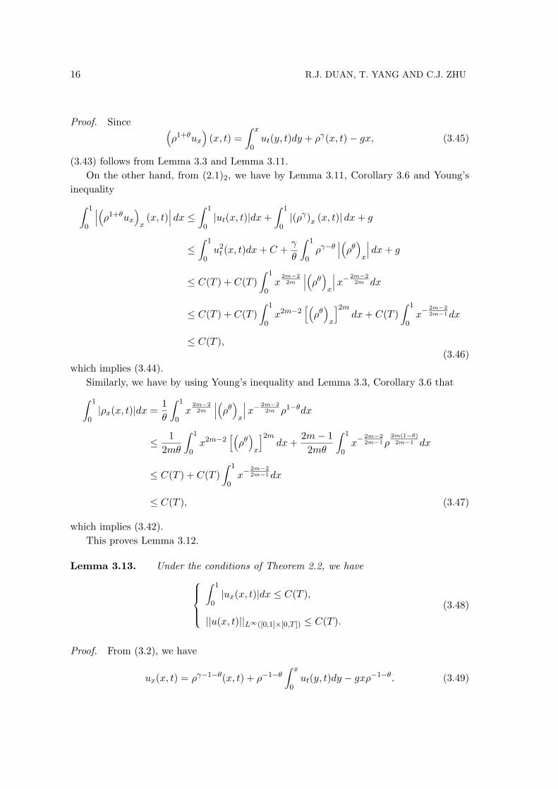
16 R.J. DUAN, T. YANG AND C.J. ZHU
Proof. Since (ρ1+θux
)(x, t) =
∫ x
0ut(y, t)dy + ργ(x, t)− gx, (3.45)
(3.43) follows from Lemma 3.3 and Lemma 3.11.On the other hand, from (2.1)2, we have by Lemma 3.11, Corollary 3.6 and Young’s
inequality∫ 1
0
∣∣∣(ρ1+θux
)x(x, t)
∣∣∣ dx ≤ ∫ 1
0|ut(x, t)|dx+
∫ 1
0|(ργ)x (x, t)| dx+ g
≤∫ 1
0u2
t (x, t)dx+ C +γ
θ
∫ 1
0ργ−θ
∣∣∣(ρθ)
x
∣∣∣ dx+ g
≤ C(T ) + C(T )∫ 1
0x
2m−22m
∣∣∣(ρθ)
x
∣∣∣x− 2m−22m dx
≤ C(T ) + C(T )∫ 1
0x2m−2
[(ρθ)
x
]2mdx+ C(T )
∫ 1
0x−
2m−22m−1dx
≤ C(T ),(3.46)
which implies (3.44).Similarly, we have by using Young’s inequality and Lemma 3.3, Corollary 3.6 that∫ 1
0|ρx(x, t)|dx =
1θ
∫ 1
0x
2m−22m
∣∣∣(ρθ)
x
∣∣∣x− 2m−22m ρ1−θdx
≤ 12mθ
∫ 1
0x2m−2
[(ρθ)
x
]2mdx+
2m− 12mθ
∫ 1
0x−
2m−22m−1 ρ
2m(1−θ)2m−1 dx
≤ C(T ) + C(T )∫ 1
0x−
2m−22m−1dx
≤ C(T ), (3.47)
which implies (3.42).This proves Lemma 3.12.
Lemma 3.13. Under the conditions of Theorem 2.2, we have∫ 1
0|ux(x, t)|dx ≤ C(T ),
||u(x, t)||L∞([0,1]×[0,T ]) ≤ C(T ).
(3.48)
Proof. From (3.2), we have
ux(x, t) = ργ−1−θ(x, t) + ρ−1−θ∫ x
0ut(y, t)dy − gxρ−1−θ. (3.49)

Navier-Stokes Equations with Vacuum 17
By Lemma 3.11 and Holder’s inequality, we have∫ 1
0|ux(x, t)|dx ≤
∫ 1
0ργ−1−θdx+
∫ 1
0ρ−1−θ
∫ x
0|ut(y, t)|dydx+ g
∫ 1
0xρ−1−θdx
≤∫ 1
0ργ−1−θdx+
∫ 1
0ρ−1−θx
12dx
(∫ 1
0u2
tdx
) 12
+ g
∫ 1
0xρ−1−θdx
≤∫ 1
0ργ−1−θdx+ C(T )
∫ 1
0x
12 ρ−1−θdx. (3.50)
The next we will prove (3.48)1.Case 1. If γ − 1− θ < 0, then we have by Lemma 3.10∫ 1
0ργ−1−θ(x, t)dx ≤ C(T )
∫ 1
0x(γ−1−θ)(1+k3)dx.
Sincek3 ≤
12θ− 1− 1
(2m− 1)θ,
we have for γ > 1
(γ − 1− θ)(1 + k3) ≥ −1 + θ − γ
2θ+
1 + θ − γ
(2m− 1)θ> −1 + θ − γ
2θ> −1.
Therefore ∫ 1
0ργ−1−θ(x, t)dx ≤ C(T ). (3.51)
Case 2. If γ − 1− θ ≥ 0, we can also obtain (3.51).On the other hand, by Corollary 3.9 and Lemma 3.10, we have∫ 1
0x
12 ρ−1−θdx ≤ max
[0,1]
x
12− 1
2m−1 ρ−θ∫ 1
0x
12m−1 ρ−1dx
≤ C(T ) max[0,1]
x
12− 1
2m−1 ρ−θ
≤ C(T ) max[0,1]
x12− 1
2m−1−θ(1+k3). (3.52)
By k3 ≤ 12θ − 1− 1
(2m−1)θ , we have
12− 1
2m− 1− θ(1 + k3) ≥ 0.
Therefore ∫ 1
0x
12 ρ−1−θdx ≤ C(T ). (3.53)
Then (3.50), (3.51) and (3.53) show (3.48)1.On the other hand, by using Sobolev’s embedding theorem W 1,1([0, 1]) → L∞([0, 1])
and Cauchy-Schwarz inequality, we have from (3.48)1 and Lemma 3.2
||u(x, t)||L∞([0,1]×[0,T ]) ≤∫ 1
0|u(x, t)|dx+
∫ 1
0|ux(x, t)|dx ≤ C(T ).

18 R.J. DUAN, T. YANG AND C.J. ZHU
This completes the proof of Lemma 3.13.Our last lemma in this section is about the L1-continuity of terms in the equations
(2.1) with respect to time.
Lemma 3.14. Under the conditions of Theorem 2.2, we have for 0 < s < t ≤ T that∫ 1
0|ρ(x, t)− ρ(x, s)|2dx ≤ C(T )|t− s|, (3.54)∫ 1
0|u(x, t)− u(x, s)|2dx ≤ C(T )|t− s|, (3.55)∫ 1
0
∣∣∣(ρ1+θux
)(x, t)−
(ρ1+θux
)(x, s)
∣∣∣2 dx ≤ C(T )|t− s|. (3.56)
Proof. We first prove (3.54). To do this, using (2.1)1, Holder’s inequality and Lemma3.2, Lemma 3.3, we have∫ 1
0|ρ(x, t)− ρ(x, s)|2dx =
∫ 1
0
∣∣∣∣∫ t
sρt(x, η)dη
∣∣∣∣2 dx=∫ 1
0
∣∣∣∣∫ t
s(ρ2ux)(x, η)dη
∣∣∣∣2 dx≤ |t− s|
∫ t
s
∫ 1
0
(ρ4u2
x
)(x, η)dxdη
≤ |t− s|∫ t
0max[0,1]
(ρ3+θ
) ∫ 1
0
(ρ1+θu2
x
)(x, η)dxdη
≤ C(T )|t− s|,
which implies (3.54).Secondly, we have by Holder’s inequality and Lemma 3.11 that∫ 1
0|u(x, t)− u(x, s)|2dx =
∫ 1
0
∣∣∣∣∫ t
sut(x, η)dη
∣∣∣∣2 dx≤ |t− s|
∫ t
s
∫ 1
0u2
t (x, η)dxdη
≤ C(T )|t− s|.
So (3.55) follows.Finally, we prove (3.56). For this, we first obtain from Holder’s inequality that∫ 1
0
∣∣∣(ρ1+θux
)(x, t)−
(ρ1+θux
)(x, s)
∣∣∣2 dx=∫ 1
0
∣∣∣∣∫ t
s
(ρ1+θux
)t(x, η)dη
∣∣∣∣2 dx≤ |t− s|
∫ t
s
∫ 1
0
[(ρ1+θux
)t(x, η)
]2dxdη. (3.57)

Navier-Stokes Equations with Vacuum 19
On the other hand, from (2.1)1, we have(ρ1+θux
)t(x, t) =
(ρ1+θuxt
)(x, t) + (1 + θ)
(ρθρtux
)(x, t)
=(ρ1+θuxt
)(x, t)− (1 + θ)
(ρ2+θu2
x
)(x, t). (3.58)
Therefore, using Cauchy-Schwarz inequality, we have from Lemma 3.2, Lemma 3.3, Lemma3.11 and Lemma 3.12 that∫ t
s
∫ 1
0
[(ρ1+θux
)t(x, η)
]2dxdη ≤ C
∫ t
0
∫ 1
0ρ2+2θu2
xtdxdη + C
∫ t
0
∫ 1
0ρ4+2θu4
xdxdη
≤ C
∫ t
0max[0,1]
(ρ1+θ
) ∫ 1
0ρ1+θu2
xtdxdη
+C∫ t
0max[0,1]
(ρ1+θux
)2max[0,1]
(ρ1−θ
) ∫ 1
0ρ1+θu2
xdxdη
≤ C(T ).
This and (3.57) implies (3.56). The proof of Lemma 3.14 is completed.
4. Construction of weak solution
To construct a weak solution to the initial boundary value problem (2.1)-(2.4), we applythe line method as in [18], which can be described as follows. For any given positive integerN , let h = 1
N . Discretizing the derivatives with respect to x in (2.1), we obtain the systemof 2N ordinary differential equations
d
dtρh2n(t) +
(ρh2n(t)
)2 uh2n+1(t)− uh
2n−1(t)h
= 0,
d
dtuh
2n−1(t) +P (ρh
2n(t))− P (ρh2n−2(t))
h
=1h2
G(ρh
2n(t))(uh2n+1(t)− uh
2n−1(t))−G(ρh2n−2(t))(u
h2n−1(t)− uh
2n−3(t))
+ g,
(4.1)with the boundary condition
ρh0(t) = uh
2N+1(t) = 0, (4.2)
and the initial data ρh2n(0) = ρ0
(2n · h
2
),
uh2n−1(0) = u0
((2n− 1) · h
2
),
(4.3)
where n = 1, 2, · · · , N and G(ρ) = µ(ρ)ρ. When n = 1, the second term in the right handof (4.1)2 is regarded as
G(ρh0(t))
uh1(t)− uh
−1(t)h2
= 0.

20 R.J. DUAN, T. YANG AND C.J. ZHU
To the end, we will use (ρ2n, u2n−1) to replace (ρh2n, u
h2n−1) without any ambiguity.
By using the arguments in [19, 21], we can prove the following lemmas for obtaining theuniform estimate of the approximate solutions to (4.1)-(4.3) with respect to h. Since theyare the same as or similar to those in [19, 21], we omit the proofs for brevity. Interestedreaders please refer to [19, 21]. In the following, we consider the solutions to (4.1)-(4.3)for 0 ≤ t ≤ T where T > 0 is any constant.
Lemma 4.1. Let (ρ2n(t), u2n−1(t)), n = 1, 2, · · · , N , be the solution to (4.1)-(4.3).Then there exists C(T ) independent of h such that
N∑n=1
(12u2
2n−1(t) +1
γ − 1ργ−12n (t) +
gnh
ρ2n(t)
)h+
∫ t
0
N∑n=1
G(ρ2n(s))(u2n+1(s)− u2n−1(s)
h
)2
hds
=N∑
n=1
(12u2
2n−1(0) +1
γ − 1ργ−12n (0) +
gnh
ρ2n(0)
)h ≤ C.
(4.4)As a consequence of (4.4), the problem (4.1)-(4.3) has a unique global solution for any
given h.
Lemma 4.2. For the positive integer m defined by (2.5), we have
ρ2n(t) ≤ C(T ), (4.5)
and
N∑n=1
u2m2n−1(t)h+
∫ t
0
N∑n=1
u2m−22n−1 (s)ρ1+θ
2n (s)(u2n−1(s)− u2n−3(s)
h
)2
hds ≤ C(T ). (4.6)
Lemma 4.3. For the positive integer m defined by (2.5), we have
N∑n=1
(nh)2m−2
(ρθ2n(t)− ρθ
2n−2(t)h
)2m
h ≤ C(T ), (4.7)
N∑n=1
(nh)1
2m−1 ρ−12n (t)h ≤ C(T ), (4.8)
N∑n=1
[d
dtu2n−1(t)
]2h+
∫ t
0
N∑n=1
ρ1+θ2n (s)
(ddtu2n−1(s)− d
dtu2n−3(s)h
)2
hds ≤ C(T ), (4.9)
andρ2n(t) ≥ C(T )(nh)1+k3 , (4.10)
where k3 satisfies (2.11).Based on Lemma 4.1, Lemma 4.2 and Lemma 4.3, similar to the arguments in [18,
19, 21] and those in the proof of Lemma 3.12, Lemma 3.13, Lemma 3.14, we can get thefollowing estimates.
Navier-Stokes Equations with Vacuum 21
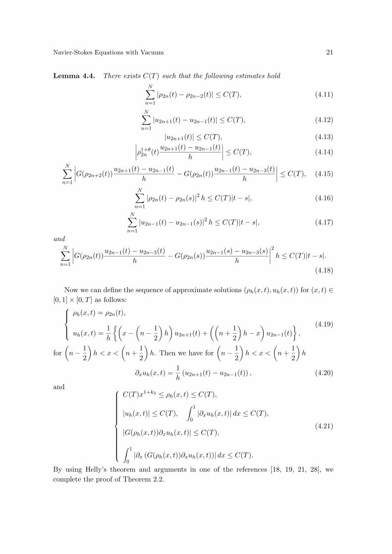
Lemma 4.4. There exists C(T ) such that the following estimates holdN∑
n=1
|ρ2n(t)− ρ2n−2(t)| ≤ C(T ), (4.11)
N∑n=1
|u2n+1(t)− u2n−1(t)| ≤ C(T ), (4.12)
|u2n+1(t)| ≤ C(T ), (4.13)∣∣∣∣ρ1+θ2n (t)
u2n+1(t)− u2n−1(t)h
∣∣∣∣ ≤ C(T ), (4.14)
N∑n=1
∣∣∣∣G(ρ2n+2(t))u2n+1(t)− u2n−1(t)
h−G(ρ2n(t))
u2n−1(t)− u2n−3(t)h
∣∣∣∣ ≤ C(T ), (4.15)
N∑n=1
|ρ2n(t)− ρ2n(s)|2 h ≤ C(T )|t− s|, (4.16)
N∑n=1
|u2n−1(t)− u2n−1(s)|2 h ≤ C(T )|t− s|, (4.17)
andN∑
n=1
∣∣∣∣G(ρ2n(t))u2n−1(t)− u2n−3(t)
h−G(ρ2n(s))
u2n−1(s)− u2n−3(s)h
∣∣∣∣2 h ≤ C(T )|t− s|.
(4.18)
Now we can define the sequence of approximate solutions (ρh(x, t), uh(x, t)) for (x, t) ∈[0, 1]× [0, T ] as follows:
ρh(x, t) = ρ2n(t),
uh(x, t) =1h
(x−
(n− 1
2
)h
)u2n+1(t) +
((n+
12
)h− x
)u2n−1(t)
,
(4.19)
for(n− 1
2
)h < x <
(n+
12
)h. Then we have for
(n− 1
2
)h < x <
(n+
12
)h
∂xuh(x, t) =1h
(u2n+1(t)− u2n−1(t)) , (4.20)
and
C(T )x1+k3 ≤ ρh(x, t) ≤ C(T ),
|uh(x, t)| ≤ C(T ),∫ 1
0|∂xuh(x, t)| dx ≤ C(T ),
|G(ρh(x, t))∂xuh(x, t)| ≤ C(T ),
∫ 1
0|∂x (G(ρh(x, t))∂xuh(x, t))| dx ≤ C(T ).
(4.21)
By using Helly’s theorem and arguments in one of the references [18, 19, 21, 28], wecomplete the proof of Theorem 2.2.

22 R.J. DUAN, T. YANG AND C.J. ZHU
5. Uniqueness of weak solution
In this section, we will prove the uniqueness of the weak solution constructed in Section4. To do this, we first give two lemmas.
Lemma 5.1. For 0 < θ < 12 , let
l1 = 1 + θ − 12(1 + k3)
(≤ 1), (5.1)
where k3 is defined by (2.11). Then there exists some constant C(T ) such that
||(ρl1ux)(x, t)||L∞([0,1]×[0,T ]) ≤ C(T ). (5.2)
Proof. We first notice from (2.11)
−12< l1 − 1− θ < −θ < 0.
Then from (3.2), Lemma 3.3, Lemma 3.10 and Lemma 3.11, we have by Holder’s inequalitythat
|(ρl1ux)(x, t)| ≤ ργ+l1−1−θ + ρl1−1−θ∫ x
0|ut(y, t)|dy + gxρl1−1−θ
≤ C(T ) + ρl1−1−θ(∫ x
0u2
t (y, t)dx) 1
2
x12 + gxρl1−1−θ
≤ C(T ) + C(T )x12+(1+k3)(l1−1−θ) + Cx1+(1+k3)(l1−1−θ). (5.3)
From (5.1), we have
12
+ (1 + k3)(l1 − 1− θ) = 0, 1 + (1 + k3)(l1 − 1− θ) =12> 0.
This and (5.3) show (5.2). The proof of Lemma 5.1 is completed.
Since
0 ≤ ρ0(x) ≤ Cxα, 0 < α < 1, 0 ≤ x ≤ 1, (5.4)
therefore, similar to the proof in [30], we have the following result.
Lemma 5.2. Under conditions (A1)′-(A3)′, we have
ρ(x, t) ≤ C(T )xα, (5.5)
for 0 < x < 1, 0 < t ≤ T .

Navier-Stokes Equations with Vacuum 23
Proof of Theorem 2.4. Let (ρ1, u1)(x, t) and (ρ2, u2)(x, t) be two solutions tothe initial boundary value problem (2.1)-(2.4) as described in Definition 2.1. Then fromLemma 5.1 and Lemma 5.2, we have for i = 1, 2 ||(ρl1
i ∂xui)(x, t)||L∞([0,1]×[0,T ]) ≤ C(T ),
0 ≤ ρi(x, t) ≤ C(T )xα.(5.6)
Let φ(x, t) = (ρ1 − ρ2)(x, t),
ψ(x, t) =∫ x
0(u1 − u2)(y, t)dy,
(5.7)
for 0 ≤ x ≤ 1 and 0 ≤ t ≤ T .By the boundary condition (2.2), we have
φ(0, t) = ψ(0, t) = ψt(0, t) = ψx(1, t) = 0 (5.8)
for 0 ≤ t ≤ T .In the following, we may assume that (ρ1, u1)(x, t) and (ρ2, u2)(x, t) are suitably smooth
since the following estimates are valid for the solutions with the regularity indicated inTheorem 2.2 by using the Friedrichs mollifier.
It follows from (2.1) and (5.7) (φ
ρ1ρ2
)t
+ ψxx = 0, (5.9)
and
ψt +ργ1 − ργ
2
ρ1 − ρ2φ = ρ1+θ
1 ψxx +ρ1+θ1 − ρ1+θ
2
ρ1 − ρ2φu2x. (5.10)
Multiplying (5.9) by 2ρl21 ρ
−12 φ, we have
(ρ−1+l21 ρ−2
2 φ2)t + (1 + l2)ρl21 ρ
−22 φ2u1x + 2ρl2
1 ρ−12 φψxx = 0, (5.11)
whereθ ≤ l2 ≤
(1
1 + k3− 2θ
)α
1 + k3− θ. (5.12)
The proof of the existence of l2 is given by Remark 5.3.Integrating (5.11) with respect to x over [0, 1] and using Cauchy-Schwarz inequality,
we have
d
dt
∫ 1
0ρ−1+l21 ρ−2
2 φ2dx
≤ C
∫ 1
0ρl2−l11 ρ−2
2 φ2|ρl11 u1x|dx+
14
∫ 1
0ρ1+θ1 ψ2
xxdx+ C
∫ 1
0ρ2l2−1−θ1 ρ−2
2 φ2dx
≤ C(T )∫ 1
0ρl2−l11 ρ−2
2 φ2dx+14
∫ 1
0ρ1+θ1 ψ2
xxdx+ C
∫ 1
0ρ2l2−1−θ1 ρ−2
2 φ2dx. (5.13)

24 R.J. DUAN, T. YANG AND C.J. ZHU
From (5.1) and (5.12), we havel2 − l1 ≥ −1 + l2
and2l2 − 1− θ ≥ −1 + l2.
Therefore
d
dt
∫ 1
0ρ−1+l21 ρ−2
2 φ2dx ≤ C(T )∫ 1
0ρ−1+l21 ρ−2
2 φ2dx+14
∫ 1
0ρ1+θ1 ψ2
xxdx. (5.14)
Multiplying (5.10) by ψxx, we have(12ψ2
x
)t+ ρ1+θ
1 ψ2xx =
ργ1 − ργ
2
ρ1 − ρ2φψxx −
ρ1+θ1 − ρ1+θ
2
ρ1 − ρ2φu2xψxx + (ψtψx)x. (5.15)
Integrating (5.15) with respect to x over [0, 1] and using Cauchy-Schwarz inequality, wehave from (5.6), (5.8), Lemma 3.10 and noticing l1 > 0
12d
dt
∫ 1
0ψ2
xdx+∫ 1
0ρ1+θ1 ψ2
xxdx
=∫ 1
0
ργ1 − ργ
2
ρ1 − ρ2φψxxdx−
∫ 1
0
ρ1+θ1 − ρ1+θ
2
ρ1 − ρ2φu2xψxxdx
≤ 14
∫ 1
0ρ1+θ1 ψ2
xxdx+ C(T )∫ 1
0ρ−1−θ1 φ2dx+ C(T )
∫ 1
0ρ−1−θ1 φ2u2
2xdx
≤ 14
∫ 1
0ρ1+θ1 ψ2
xxdx+ C(T ) max[0,1]
(ρ−θ−l21 ρ2
2
) ∫ 1
0ρ−1+l21 ρ−2
2 φ2dx
+C(T ) max[0,1]
(ρ−θ−l21 ρ2
2u22x
) ∫ 1
0ρ−1+l21 ρ−2
2 φ2dx
≤ 14
∫ 1
0ρ1+θ1 ψ2
xxdx+ C(T ) max[0,1]
(ρ−θ−l21 ρ2
2
) ∫ 1
0ρ−1+l21 ρ−2
2 φ2dx
+C(T ) max[0,1]
(ρ−θ−l21 ρ2−2l1
2
)max[0,1]
(ρl12 u2x
)2∫ 1
0ρ−1+l21 ρ−2
2 φ2dx
≤ 14
∫ 1
0ρ1+θ1 ψ2
xxdx+ C(T ) max[0,1]
(x(2−2l1)α−(θ+l2)(1+k3)
) ∫ 1
0ρ−1+l21 ρ−2
2 φ2dx. (5.16)
From (5.1) and (5.12), we have
(2− 2l1)α− (θ + l2)(1 + k3) ≥ 0.
Therefore12d
dt
∫ 1
0ψ2
xdx+∫ 1
0ρ1+θ1 ψ2
xxdx
≤ 14
∫ 1
0ρ1+θ1 ψ2
xxdx+ C(T )∫ 1
0ρ−1+l21 ρ−2
2 φ2dx. (5.17)

Navier-Stokes Equations with Vacuum 25
Thus (5.14) and (5.17) show
d
dt
(∫ 1
0ρ−1+l21 ρ−2
2 φ2dx+12
∫ 1
0ψ2
xdx
)+
12
∫ 1
0ρ1+θ1 ψ2
xxdx
≤ C(T )∫ 1
0ρ−1+l21 ρ−2
2 φ2dx. (5.18)
By using Gronwall’s inequality, we have for any t > 0∫ 1
0ρ−1+l21 ρ−2
2 φ2dx = 0 (5.19)
and ∫ 1
0ψ2
xdx = 0. (5.20)
This proves Theorem 2.4.
Remark 5.3. There exists some constant l2 which satisfies (5.12).In fact, (5.12) is equivalent to
(1 + k3)2 + (1 + k3)α−α
2θ≤ 0, (5.21)
which implies
1 + k3 ≤ −α2
+12
√α2 +
2αθ. (5.22)
From (2.11) and (5.22), we have
2m− 12m− 2mθ − 1
+α
2≤ 1
2
√α2 +
2αθ, (5.23)
i.e.,
α ≥ 2(2m− 1)2θ(2m− 2mθ − 1)(2m− 6mθ + 2θ − 1)
. (5.24)
Furthermore, (5.24) can be rewritten as
4(3αθ2 − (4α+ 2)θ + α)m2 − 4(αθ2 − (3α+ 2)θ + α)m+ α− (2α+ 2)θ ≥ 0. (5.25)
When 0 < θ <α
1 + 2α+√
1 + 4α+ α2, we have
3αθ2 − (4α+ 2)θ + α > 0. (5.26)
From the assumption (A3)′ and (5.26), we see (5.25) holds. Now let
2mθ2m(1− θ)− 1
≤ k3 ≤ min
12θ− 1− 1
(2m− 1)θ, −α
2− 1 +
12
√α2 +
2αθ
, (5.27)
that is to say, we may choose m so large that (2.14) is satisfied. Then (5.22) holds. Sothere exists some constant l2 such that (5.12) hold.

26 R.J. DUAN, T. YANG AND C.J. ZHU
Remark 5.4. When α is sufficiently close to 1, then θ may be sufficiently close to1−
√6
3 .
Acknowledgement: The research of the second author was supported by Hong KongRGC Competitive Earmarked Research Grant CityU 102703 and the National NaturalScience Foundation of China #10329101, respectively. The research of the third authorwas supported by Program for New Century Excellent Talents in University #NCET-04-0745, the Key Project of the National Natural Science Foundation of China #10431060and the Key Project of Chinese Ministry of Education #104128.
References
[1] R. Balian, From microphysics to macrophysics, Texts and monographs in physics,Springer, 1982.
[2] G.Q. Chen, D. Hoff and K. Trivisa, Global solutions of the compressible Navier-Stokesequations with large discontinuous initial data, Comm. Partial Differential Equations,25(2000), 2233-2257.
[3] G.Q. Chen and M. Kratka, Global solutions to the Navier-Stokes equations for com-pressible heat-conducting flow with symmetry and free boundary, Comm. PartialDifferential Equations, 27(2002), 907-943.
[4] D.Y. Fang, T. Zhang, A note on compressible Navier-Stokes equations with vacuumstate in one dimension, Nonlinear Anal., TMA, 58(2004), 719-731.
[5] H. Grad, Asymptotic theory of the Boltzmann equation II. In: Rarefied gas dynamics,1(ed. J. Laurmann), New York Academic Press(1963), 26-59.
[6] D. Hoff, Strong convergence to global solutions for multidimensional flows of com-pressible, viscous fluids with polytropic equations of state and discontinuous initialdata, Arch. Rat. Mech. Anal., 132(1995), 1-14.
[7] D. Hoff and T.-P. Liu, The inviscid limit for the Navier-Stokes equations of compress-ible isentropic flow with shock data, Indiana Univ. Math. J., 38(1989), 861-915.
[8] D. Hoff and D. Serre, The failure of continuous dependence on initial data for theNavier-Stokes equations of compressible flow, SIAM J. Appl. Math., 51(1991), 887-898.
[9] D. Hoff and J. Smoller, Non-formation of vacuum states for compressible Navier-Stokes equations, Comm. Math. Phys., 216(2001), 255–276.
[10] S. Jiang, Global smooth solutions of the equations of a viscous, heat-conducting, one-dimensional gas with density-dependent viscosity, Math. Nachr., 190(1998), 169-183.

Navier-Stokes Equations with Vacuum 27
[11] S. Jiang, Z.P. Xin and P. Zhang, Global weak solutions to 1D compressible isentropicNavier-Stokes equations with density-dependent viscosity, preprint 1999.
[12] S. Kawashima and T. Nishida , The initial-value problems for the equations of viscouscompressible and perfect compressible fluids, RIMS, Kokyuroku 428, Kyoto Univer-sity, Nonlinear Functional Analysis, June 1981, 34-59.
[13] P.L. Lions, Mathematical Topics in Fluid Mechanics, Vol. 1, 2, (1998), ClarendonPress-Oxford.
[14] T.-P. Liu, Z. Xin and T. Yang, Vacuum states of compressible flow, Discrete andContinuous Dynamical Systems, 4(1998), 1-32.
[15] T. Luo, Z. Xin and T. Yang, Interface behavior of compressible Navier-Stokes equa-tions with vacuum, SIAM J. Math. Anal., 31(2000), 1175-1191.
[16] T. Makino, On a local existence theorem for the evolution equations of gaseous stars,“Patterns and wave-qualitative analysis of nonlinear differential equations”, Ed. T.Nishida, M. Mimura and H. Fujii, North-Holland, 1986, 459-479.
[17] T. Nishida, Equations of fluid dynamics-free surface problems, Comm. Pure Appl.Math., XXXIX(1986), 221-238.
[18] T. Nishida, Equations of motion of compressible viscous fluids, Patterns and Waves–Qualitative Analysis of Nonlinear Differential Equations, (1986), 97-128.
[19] M. Okada, Free boundary value problems for the equation of one-dimensional motionof viscous gas, Japan J. Appl. Math., 6(1989), 161-177.
[20] M. Okada and T. Makino, Free boundary problem for the equations of sphericallysymmetrical motion of viscous gas, Japan J. Indust. Appl. Math., 10(1993), 219-235.
[21] M. Okada, S. Matusu-Necasova and T. Makino, Free boundary problem for the equa-tion of one-dimensional motion of compressible gas with density-dependent viscosity,Ann. Univ. Ferrara Sez, VII-Sc.Mat., 48(2002), 1-20.
[22] D. Serre, Sur l’equation mondimensionnelle d’un fluide visqueux, compressible etconducteur de chaleur, Comptes rendus Acad. des Sciences. 303(1986), 703-706.
[23] I. Straskraba, A.A. Zlotnik, Global properties of solutions to 1D-viscous compressiblebaratropic fluid equations with density dependent viscosity, Z. angew. Math. Phys.,54(2003), 593-607.
[24] I. Straskraba, Global analysis of 1-D Navier-Stokes equations with density dependentviscosity, In: Navier-Stokes equations and related nonlinear problems (H. Amann etal., eds.) VSP Utrecht, TEV Vilnius (1997), 371-390.

28 R.J. DUAN, T. YANG AND C.J. ZHU
[25] Z. Xin, Blow-up of smooth solutions to the compressible Navier-Stokes equations withcompact density, Comm. Pure Appl. Math., 51(1998), 229-240.
[26] S.W. Vong, T. Yang and C.J. Zhu, Compressible Navier-Stokes equations with de-generate viscosity coefficient and vacuum (II), J. Differential Equations, 192(2003),475-501.
[27] T. Yang, Some recent results on compressible flow with vacuum, Taiwanese J. Math.,4(2000), 33-44.
[28] T. Yang, Z.A. Yao and C.J. Zhu, Compressible Navier-Stokes equations with density-dependent viscosity and vacuum, Comm. Partial Differential Equations, 26(2001),965-981.
[29] T. Yang and H.J. Zhao, A vacuum problem for the one-dimensional compressibleNavier-Stokes equations with density-dependent viscosity, J. Differential Equations,184(2002), 163-184.
[30] T. Yang and C.J. Zhu, Compressible Navier-Stokes equations with degenerate viscos-ity coefficient and vacuum, Comm. Math. Phys., 230(2002), 329-363.
[31] A.A. Zlonik, Uniform estimates and stabilization of symmetric solutions of a systemof quasilinear equations, Diff. Equations 36(2000), 701-716.


![On the Vanishing Viscosity Limit for the 3D Navier-Stokes ...Dirichlet boundary conditions [17]. For the mathematical rigorous analysis of the Navier-Stokes equations with Naiver-type](https://img.pdfslide.us/doc/110x75/6121ba9b8b23fb1a5910c548/on-the-vanishing-viscosity-limit-for-the-3d-navier-stokes-dirichlet-boundary.jpg)


![Eindhoven University of Technology · arXiv:0906.4281v2 [math.PR] 10 Dec 2009 ERGODICITY OF THE 3D STOCHASTIC NAVIER-STOKES EQUATIONS DRIVEN BY MILDLY DEGENERATE NOISE MARCO ROMITO](https://img.pdfslide.us/doc/110x75/60a598a85c715c0b04414de5/eindhoven-university-of-technology-arxiv09064281v2-mathpr-10-dec-2009-ergodicity.jpg)

![Journal of Computational Physicsby Zhou and coworkers to solve the Navier–Stokes equations with discontinuous viscosity and density [40]. Recently, the MIB method has been extended](https://img.pdfslide.us/doc/110x75/5f48412f2a4fb63ddc605ebc/journal-of-computational-physics-by-zhou-and-coworkers-to-solve-the-navierastokes.jpg)