NAVAL POSTGRADUATE SCHOOL · The separately excited DC motor was investigated to develop the equations necessary to produce the model. Once the required equations were understood,

NAVAL

POSTGRADUATE

SCHOOL

MONTEREY, CALIFORNIA

THESIS

Approved for public release; distribution is unlimited

EMULATION OF WIND POWER WITH A DC MACHINE TO PROVIDE INPUT TO A DOUBLY-FED

INDUCTION MACHINE

by

Jonathan T. Hines

March 2012 Thesis Advisors: Alexander L. Julian Giovanna Oriti

THIS PAGE INTENTIONALLY LEFT BLANK

i

REPORT DOCUMENTATION PAGE Form Approved OMB No. 0704-0188 Public reporting burden for this collection of information is estimated to average 1 hour per response, including the time for reviewing instruction, searching existing data sources, gathering and maintaining the data needed, and completing and reviewing the collection of information. Send comments regarding this burden estimate or any other aspect of this collection of information, including suggestions for reducing this burden, to Washington headquarters Services, Directorate for Information Operations and Reports, 1215 Jefferson Davis Highway, Suite 1204, Arlington, VA 22202-4302, and to the Office of Management and Budget, Paperwork Reduction Project (0704-0188) Washington DC 20503. 1. AGENCY USE ONLY (Leave blank)

2. REPORT DATE March 2012

3. REPORT TYPE AND DATES COVERED Master’s Thesis

4. TITLE AND SUBTITLE Emulation of Wind Power with a DC Machine to Provide Input to a Doubly-Fed Induction Machine

5. FUNDING NUMBERS

6. AUTHOR(S) Jonathan T. Hines 7. PERFORMING ORGANIZATION NAME(S) AND ADDRESS(ES)

Naval Postgraduate School Monterey, CA 93943-5000

8. PERFORMING ORGANIZATION REPORT NUMBER

9. SPONSORING /MONITORING AGENCY NAME(S) AND ADDRESS(ES) N/A

10. SPONSORING/MONITORING AGENCY REPORT NUMBER

11. SUPPLEMENTARY NOTES The views expressed in this thesis are those of the author and do not reflect the official policy or position of the Department of Defense or the U.S. Government. IRB Protocol number ______N/A______.

12a. DISTRIBUTION / AVAILABILITY STATEMENT Approved for public release; distribution is unlimited

12b. DISTRIBUTION CODE A

13. ABSTRACT (maximum 200 words) The behavioral modeling of a separately excited direct current (DC) motor as a prime mover for a doubly-fed induction machine (DFIM) is studied in this thesis. The output torque of the DC motor is computed in the simulation under controlled parameters. The input to the DFIM, used as a doubly-fed induction generator (DFIG), is taken from the DC motor. In theory, the combination of the two machines can be used to emulate various wind patterns and their expected electrical returns for a given DFIM-based wind turbine.

A Simulink model was created to appropriately emulate the operation of the DC machine. That model was then incorporated into an existing model of a DFIM. The resulting simulations are compared to system operating data to determine if machine speed is being correctly modeled. The speeds determined by the simulator accurately track those that are gathered from lab data.

Operating speeds of the system were mapped to historical wind speeds in a geographical area. Output power of the DC motor for the different operating speeds was calculated and plotted. The data confirmed the theory of the proportionality of the rotational output power of a DC motor.

14. SUBJECT TERMS Direct Current (DC) Motor, Doubly-fed induction machine (DFIM), Doubly-fed induction generator (DFIG), Wind Power, Simulink Model

15. NUMBER OF PAGES

91 16. PRICE CODE

17. SECURITY CLASSIFICATION OF REPORT

Unclassified

18. SECURITY CLASSIFICATION OF THIS PAGE

Unclassified

19. SECURITY CLASSIFICATION OF ABSTRACT

Unclassified

20. LIMITATION OF ABSTRACT

UU NSN 7540-01-280-5500 Standard Form 298 (Rev. 2-89) Prescribed by ANSI Std. 239-18

ii


iii

Approved for public release; distribution is unlimited

EMULATION OF WIND POWER WITH A DC MACHINE TO PROVIDE INPUT TO A DOUBLY-FED INDUCTION MACHINE

Jonathan T. Hines Lieutenant, United States Navy B.S., Auburn University, 2005

Submitted in partial fulfillment of the requirements for the degree of

MASTER OF SCIENCE IN ELECTRICAL ENGINEERING

from the

NAVAL POSTGRADUATE SCHOOL March 2012

Author: Jonathan T. Hines

Approved by: Alexander L. Julian Thesis Advisor

Giovanna Oriti Thesis Advisor

R. Clark Robertson Chair, Department of Electrical and Computer Engineering

iv


v

ABSTRACT

The behavioral modeling of a separately excited direct current (DC) motor as a prime

mover for a doubly-fed induction machine (DFIM) is studied in this thesis. The output

torque of the DC motor is computed in the simulation under controlled parameters. The

input to the DFIM, used as a doubly-fed induction generator (DFIG), is taken from the

DC motor. In theory, the combination of the two machines can be used to emulate

various wind patterns and their expected electrical returns for a given DFIM-based wind

turbine.

A Simulink model was created to appropriately emulate the operation of the DC

machine. That model was then incorporated into an existing model of a DFIM. The

resulting simulations are compared to system operating data to determine if machine

speed is being correctly modeled. The speeds determined by the simulator accurately

track those that are gathered from lab data.

Operating speeds of the system were mapped to historical wind speeds in a

geographical area. Output power of the DC motor for the different operating speeds was

calculated and plotted. The data confirmed the theory of the proportionality of the

rotational output power of a DC motor.

vi


vii

TABLE OF CONTENTS

I. INTRODUCTION AND BACKGROUND INFORMATION .................................1 A. BACKGROUND ..............................................................................................1 B. OBJECTIVE ....................................................................................................2 C. APPROACH .....................................................................................................3 D. THESIS ORGANIZATION ............................................................................3

II. SIMULATED DC MACHINE ANALYSIS...............................................................5 A. INTRODUCTION............................................................................................5 B. DC MOTOR EQUATIONS ............................................................................5

1. Basic DC Motor Theory ......................................................................5 2. DC Motor Equations for Separately-Excited Windings ...................7

C. OVERVIEW OF EQUIPMENT CONFIGURATION .................................8 D. SIMULINK MODEL .......................................................................................9 E. MODEL VALIDATION FOR ARMATURE AND FIELD

CURRENTS....................................................................................................13 F. MODEL VALIDATION FOR SPEED ........................................................14

1. Comparison between Operational Data and Simulated Data .......14 2. Results .................................................................................................16

G. MODEL VALIDATION FOR ELECTRICAL INPUT POWER .............17 1. Comparison between Operational Data and Simulated Data .......17 2. Results .................................................................................................19

H. MODELING MECHANICAL OUTPUT POWER ....................................20 I. CHAPTER SUMMARY ................................................................................21

III. MODELING WIND PROFILES..............................................................................23 A. INTRODUCTION..........................................................................................23 B. MAPPING STRATEGY FOR WIND SPEED TO DC MOTOR

SPEED .............................................................................................................23 1. Overview .............................................................................................23 2. Geographic Area Selection ................................................................23 3. Mapping Strategy...............................................................................24 4. Simulation of Different Wind Speeds ...............................................26 5. Simulation of Output Power Based on Wind Speeds .....................26 6. Analysis of Simulated Speed and Power ..........................................27

C. CHAPTER SUMMARY ................................................................................28

IV. CONCLUSIONS AND FUTURE RESEARCH ......................................................29 A. CONCLUSIONS ............................................................................................29 B. FUTURE RESEARCH ..................................................................................29

APPENDIX A .........................................................................................................................31

APPENDIX B .........................................................................................................................33

APPENDIX C .........................................................................................................................51

viii

LIST OF REFERENCES ......................................................................................................65

INITIAL DISTRIBUTION LIST .........................................................................................67

ix

LIST OF FIGURES

Figure 1. Measured and simulated system RPM vs. time. ............................................ xvi Figure 2. Measured and simulated input power vs. time.............................................. xvii Figure 3. Simulated average DC motor speed by month for wind turbine in Norfolk.xviii Figure 4. Simulated average DC motor output power by month for Norfolk. ............ xviii Figure 5. DFIG connected to wind turbine, from [2]. .......................................................1 Figure 6. DFIG connected to DC motor, from [4]. ...........................................................2 Figure 7. Elementary 2-pole DC machine, from [5]. ........................................................6 Figure 8. Equivalent circuit for separately excited DC machine, from [5]. ......................8 Figure 9. Equipment setup in lab, from [3] .......................................................................9 Figure 10. DC motor model in Simulink. ..........................................................................11 Figure 11. Measured and simulated armature and field currents. .....................................13 Figure 12. Measured system RPM vs. time.......................................................................14 Figure 13. Simulated system RPM vs. time. .....................................................................15 Figure 14. Measured and simulated system RPM vs. time. ..............................................16 Figure 15. Measured input power of DC motor vs. time. .................................................17 Figure 16. Simulated input power of DC motor vs. time. .................................................18 Figure 17. Measured and simulated input power vs. time.................................................19 Figure 18. Simulated output power of DC motor. .............................................................20 Figure 19. Simulated average DC motor speed by month for wind turbine in Norfolk. ...26 Figure 20. Simulated average DC motor output power by month for Norfolk. ................27 Figure 21. Overall DFIG system, from [3]. .......................................................................33 Figure 22. Induction Machine of Overall DFIG system, from [3]. ...................................34 Figure 23. Subsystem of Induction Machine, from [3]. ....................................................35 Figure 24. Inverse Ks transformation in Subsystem, from [3]. .........................................35 Figure 25. Inverse Ks transformation1 in Subsystem, from [3]. .......................................36 Figure 26. Subsystem1 of Induction Machine, from [3]. ..................................................37 Figure 27. Subsystem2 of Induction Machine, from [3]. ..................................................37 Figure 28. Subsystem3 of Induction Machine, from [3]. ..................................................38 Figure 29. Stator of Subsystem3, from [3]. .......................................................................38 Figure 30. Stator1 of Subsystem3, from [3]. .....................................................................39 Figure 31. Inverse Kr transformation of Induction Machine, from [3]. ............................39 Figure 32. Psi_dr of Induction Machine, from [3]. ...........................................................40 Figure 33. Psi_ds of Induction Machine, from [3]. ...........................................................40 Figure 34. Psi_md of Induction Machine, from [3]. .........................................................40 Figure 35. Psi_mq of Induction Machine, from [3]. .........................................................41 Figure 36. Psi_qr of Induction Machine, from [3]. ...........................................................41 Figure 37. Psi_qs of Induction Machine, from [3]. ...........................................................41 Figure 38. Rotor controller of Induction Machine, from [3]. ............................................42 Figure 39. AC source of Rotor Controller, from [3]. ........................................................43 Figure 40. Ks transformation of Rotor Controller, from [3]. ............................................43 Figure 41. Inverse trans of Rotor Controller, from [3]. .....................................................44 Figure 42. Rotor currents of Induction Machine, from [3]. ..............................................44

x

Figure 43. Rotor currents1 of Induction Machine, from [3]. ............................................45 Figure 44. Torque of Induction Machine, from [3]. ..........................................................45 Figure 45. Input torque of Overall DFIG system. .............................................................46 Figure 46. Separately excited DC motor of input torque. .................................................47 Figure 47. Inverse Kr transformation of Overall DFIG system, from [3]. ........................48 Figure 48. Inverse Ks transformation of Overall DFIG system, from [3].........................49 Figure 49. Torque equation of Overall DFIG system, from [3]. .......................................49

xi

LIST OF TABLES

Table 1. Values for variables used in DC motor model. ................................................10 Table 2. Monthly wind speed averages for Norfolk, Virginia, from [6]. .......................24 Table 3. Scaling of monthly average wind speed in Norfolk, Virginia, to motor

RPM. ................................................................................................................25

xii


xiii

LIST OF ACRONYMS AND ABBREVIATIONS

A Amperes

DC Direct Current

DFIG Doubly Fed Induction Generator

H Henries

ai Armature Current

fi Field Current

AAL Armature Self Inductance

AFL Mutual Inductance Between Armature and Field

FFL Field Self Inductance

2i rP Armature Losses

inP DC Machine Rotor Input Power

outP DC Machine Rotational Output Power

ar Armature Resistance

fr Field Resistance

RPM Revolutions Per Minute

ORPM Motor Operation Speed Scaled to Wind Speed

eT Output Torque of DC Machine

V Volts

av Armature Voltage Supplied to DC Motor

,a sourcev Source Armature Voltage

xiv

fv Field Voltage Supplied to DC Motor

,f sourcev Source Field Voltage

rω Rotational Speed

xv

EXECUTIVE SUMMARY

The theory of the separately excited direct current (DC) motor as a means to create a

simulated model of the machine is explored in this thesis. This model is used as an input

to a doubly-fed induction generator (DFIG) model. The model is expected to provide a

more accurate evaluation of system behavior than was previously utilized in earlier

research on this system because the earlier research did not include a detailed model of a

DC machine as is the case in the lab hardware.

The separately excited DC motor was investigated to develop the equations

necessary to produce the model. Once the required equations were understood, the model

was designed using the Simulink program. This model of the DC motor was incorporated

within a larger simulation of a DFIG system with the DC motor acting as the prime

mover.

Test runs were completed in the lab using the operational setup. Speed runs were

conducted with commanded speed beginning at 1,441 revolutions per minute (RPM) and

then shifting to 1,981 RPM. The data from these runs was output to a file that could be

incorporated into Matlab.

Next, the simulation of the overall DFIG system was run using the same

commanded speed changes. A plot was constructed of the operational speed of the

simulation versus time. The model was tested for validity by collecting data from lab

experimentation and then comparing the data to the output of the model. The resulting

speed testing plot comparing measured and simulated data is shown in Figure 1.

xvi

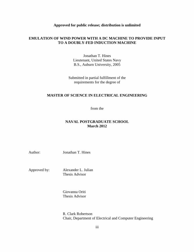
Figure 1. Measured and simulated system RPM vs. time.

The comparison of simulated speed and the measured speed of the system is

shown in Figure 1. The simulation results and the results obtained from the operational

data for the experimental run for speed are closely matched.

The power data was also gathered from the operational runs. The armature input

power from the DC motor model and that of the actual machine are shown in Figure 2.

The steady state values of the Simulink analysis closely approximate those from the

machine run. The machine model does not contain enough detail to fully simulate the

drop in power at the transition in speed, but the dip in the simulated power is similar to

that observed in the measurements.

xvii

Figure 2. Measured and simulated input power vs. time.

Next, the average monthly wind speeds for a particular area were scaled to

operational rotational speeds of the DC motor. The output power was computed using the

simulated model. The correlation between the operational speed of the DC motor and the

output power was confirmed. The plots of the scaled speed and the corresponding output

power are shown in Figures 3 and 4, respectively. Each plot begins with the values for

January at the left and shifts months every four seconds. The conversion of the wind

speed to a particular power level depends on the design of the turbine/gearbox/generator,

and no specific hardware is being represented in this thesis.

xviii

Figure 3. Simulated average DC motor speed by month for wind turbine in Norfolk.

Figure 4. Simulated average DC motor output power by month for Norfolk.

xix

In summary, a model of the separately excited DC motor was created using

Simulink. The motor model responded predictably and accurately to changes in speed.

The input power also responded accordingly leading to a predictable output power of the

system. This will allow for future research to build upon the model to perform further

analysis of the DFIG system at the Naval Postgraduate School.

xx


xxi

ACKNOWLEDGMENTS

First and foremost, I thank God for the perseverance to see this thesis through. If

not for His grace and mercy, I would have never been able to complete the task.

Thank you to all of the staff and faculty of the Naval Postgraduate School who

have facilitated the wonderful educational opportunity that I have had here. The

dedication and time of so many have contributed to my tour being such a wonderful time

for professional and personal growth. In particular, I want to thank Professor Julian for

his advice and knowledge during this process. I learned so much from you and you have

my deepest gratitude.

Finally, I must thank the three most important people in my life. To my beautiful

wife, Linda, you are my rock and my support. Without your love and encouragement,

along with your calming presence, I never would have survived the stresses of the last

two years. I am so blessed to have you. To my wonderful sons, Jonathan and Joshua,

thank you so much for your boundless enthusiasm and joy. You two could always make

me laugh and you never failed at helping me put things in perspective. Whenever I felt

down, you helped me to realize that things were never really bad as long as I had the love

of you guys and your mother.

xxii


1

I. INTRODUCTION AND BACKGROUND INFORMATION

A. BACKGROUND

Per the Energy Policy Act of 2005, the United States government is requiring that

federal agencies, including the Department of Defense (DoD), actively increase their

usage of renewable energy sources. By the year 2025, the DoD is required to produce or

procure at least 25% of its total facility energy from these sources [1]. Meeting this goal

requires an investment in various forms of technology to produce and implement

renewable sources.

Wind power is a potential source of energy that the DoD should exploit. This

would be of great help in achieving the goals of The Energy Policy Act. Wind technology

can provide a proven method of renewable energy.

Doubly-fed induction generators (DFIG) are often used in wind power generation

to supply power to a grid [2]. The turbine blades are connected to a gearbox that provides

input torque to a DFIG. A typical DFIG system is shown in Figure 5.

Figure 5. DFIG connected to wind turbine, from [2].

2

The Naval Postgraduate School has developed a wind power emulator that

replaces the turbine and associated gearbox with a direct current (DC) motor. A

simulation was created with this project to predict and explain its operation [3]. This

setup is displayed in Figure 6.

Figure 6. DFIG connected to DC motor, from [4].

B. OBJECTIVE

The objective of this thesis is to provide better predictions of the operational

speed and input torque of the machines through modeling of the DC machine. The initial

simulations in Matlab used a torque constant as input into the modeled DFIG [2]. While

this method is more than sufficient for studies of the electrical output of the DFIG itself,

it does not accurately predict the torque of the DC machine, particularly when

transitioning between different speeds. The hypothesis is that creating a full model of a

DC machine using Matlab and Simulink and providing input to the Simulink model of

the DFIG will provide a greater level of predictability of system behavior.

Verifying the relationship between output power and speed was a secondary goal

of the study. Theoretically, the DC motor can be used to model the output power and

3

torque provided by turbine blading and the gearbox [2]. The goal is to model the

rotational output power through the use of Simulink and prove the interconnection

between power and speed.

C. APPROACH

The first step in this thesis was to understand the operation of the DC machine

that was to be used. The machine in question was a separately-excited DC motor. By

leveraging previous studies, a mathematical model of the DC motor was created.

References [4], [5], [6], and [7] were used to gather this information. Next, the model of

the separately-excited DC motor was created using Simulink. The model of the DC motor

was then implemented as a replacement for the constant torque input in the DFIG

Simulink model [2]. Machine speed data, including a change in operating speed, and

output power data were obtained from equipment operation in the lab. This data was

compared to the predicted speed and predicted output power from the simulation to

validate the simulation accuracy.

D. THESIS ORGANIZATION

The theory of operation for the separately excited DC motor is covered in Chapter

II. The equations for the field and armature voltages and currents, torque, and power are

presented. The Lab-Volt 8211 DC Motor/Generator is employed, as part of an operating

DFIG system, to provide output data for later analysis. A representative model of the

Lab-Volt DC motor is created in Simulink as part of an overall DFIG system [2]. The

output data of the model is compared to the actual output of the motor to determine

accuracy of the simulation.

A wind profile from a particular geographic area is discussed in Chapter III. The

wind speeds of this profile are mapped to motor operating speeds for the simulated DC

machine. The output power of the machine is computed by the simulation based on the

different speeds of operation.

4

Conclusions are drawn about the testing results in Chapter IV. The validity of the

created model for simulations of the DFIG system is reviewed. Some possibilities for

future work to build upon this topic are also presented.

5

II. SIMULATED DC MACHINE ANALYSIS

A. INTRODUCTION

The equations that define a DC motor are reviewed in this section [5]. Using

values determined from previous research on this machine, we created a model using

Matlab’s Simulink software. The model, used as the prime mover for the DFIG

simulation, is evaluated using a specific operational profile. The speed output is

compared to the output of the actual machinery running the same profile to test the

validity of the model.

B. DC MOTOR EQUATIONS

1. Basic DC Motor Theory

DC motors have been used for many years, and the characteristics of these

machines are well understood. The overall principle behind the operation is quite simple.

A current-carrying conductor, in the presence of a magnetic field, experiences a force that

is perpendicular to both the current and the direction of the magnetic field. Using this

knowledge to produce a practical DC motor is difficult.

Figure 7 is a representation of a simple DC machine [5]. The stator poles are

wound with field windings, while the rotor has its own coil. A commutator, made up of

two semicircular copper segments, is mounted at the end of the rotor. The terminals of

the rotor coil are connected to the copper segment. Voltage is supplied to the rotor from a

stationary circuit via carbon brushes, which causes a current to flow through the rotor

coils. The commutator allows for current to be supplied in a consistent direction so that

the application of electrical torque on the rotor forces rotation in the same direction at all

times [5].

6

Figure 7. Elementary 2-pole DC machine, from [5].

The commutating action causes the rotor coils to appear as a stationary winding

with respect to the field. The magnetic axis of the rotor windings always appears

perpendicular to that of the stator windings. Because of this, there is no induction of

voltages in one winding due to a time rate of change of current in the other [5].

7

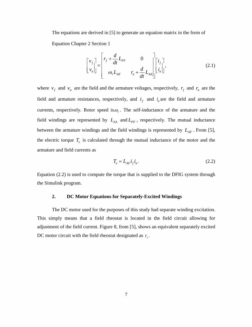
The equations are derived in [5] to generate an equation matrix in the form of

Equation Chapter 2 Section 1

0FFf

f f

a ar aAF AA

dr Lv idtdv iL r Ldt

ω

+=

+, (2.1)

where fv and av are the field and the armature voltages, respectively, fr and ar are the

field and armature resistances, respectively, and fi and ai are the field and armature

currents, respectively. Rotor speed is rω . The self-inductance of the armature and the

field windings are represented by AAL and FFL , respectively. The mutual inductance

between the armature windings and the field windings is represented by AFL . From [5],

the electric torque eT is calculated through the mutual inductance of the motor and the

armature and field currents as

.e aAF fT L i i= (2.2)

Equation (2.2) is used to compute the torque that is supplied to the DFIG system through

the Simulink program.

2. DC Motor Equations for Separately-Excited Windings

The DC motor used for the purposes of this study had separate winding excitation.

This simply means that a field rheostat is located in the field circuit allowing for

adjustment of the field current. Figure 8, from [5], shows an equivalent separately excited

DC motor circuit with the field rheostat designated as xr .

8

Figure 8. Equivalent circuit for separately excited DC machine, from [5].

The value of the field rheostat resistance must be taken into account when performing

calculations to determine motor operating characteristics.

C. OVERVIEW OF EQUIPMENT CONFIGURATION

A representation of the physical system setup is shown in Figure 9. The

specifications of the Lab-Volt motor used for this study are found in Appendix A. The

rotor of the DC motor is connected to the rotor of the DFIG to provide input torque for

the system.

The field programmable gate array (FPGA) is configured to receive various data

from the operating machinery. The output of data is relayed from the machinery to the

controlling personal computer via a universal serial bus connection. The data can be

retrieved and analyzed further at a later time.

An oscilloscope is connected to provide data analysis during the lab

experimentation. It is used to measure the various voltages and currents of interest for the

DFIG. The oscilloscope is also used to export data from the operational experiments.

9

3 phase AC grid

+

vdc-

A+ A- B+ B- C+ C-

Universal Serial Bus

+

-

vabr

vbcr

statorrotorDFIM

4 poles

Encoder

3Φ Input from grid Stator

connected to grid

Xilinx XC4VLX25 FPGA

Custom interface card

(A/D converters and digital I/O

A+ A- B+ B- C+ C-

Xilinx XC4VLX25 FPGA

Custom interface card

(A/D converters and digital I/O

vab

vbc

Stator l-l voltages

Rotor currents

θr

Oscilloscope

iar

Stator currents

ias

ibs

Run/stop

PCWeb Server

DC Motor

ch1ch2ch3ch4

Figure 9. Equipment setup in lab, from [3]

D. SIMULINK MODEL

Equations 2.1 and 2.2 were used to create the model of the DC machine in

Simulink. Measurements were taken with a multimeter to determine the field resistance

for the DFIG system. The measured and calculated values for armature resistance and

mutual inductance were taken from [4]. Rotor speed was initially commanded to 1,440

revolutions per minute (RPM) and then increased to 1,980 RPM. No method was readily

available to test for armature and field self-inductance values. Instead, a nominal value is

assumed for both the armature and field self-inductance based on information from [5].

The values used throughout the simulation process are shown in Table 1.

10

Table 1. Values for variables used in DC motor model.

Values for Simulation Variables

,f sourcev 170 V

,a sourcev 170 V

fr 6.4 Ω

ar 8.5 Ω

rω Varied between 151 and 207 radians/second

FFL 30 H

AAL Initially 180H; reduced to 30 H

AFL Initially 3 H, reduced to 2.25 H

,f refi 0.3125 A

,a refi 1.25 A

The next step in the process was to build the Simulink model of the DC motor.

The equations for field voltage and armature voltage were obtained from (2.1), to get

ff f f FF

div r i L

dt= + (2.3)

and

aa r AF f a a AA

div L i r i Ldt

ω= + + . (2.4)

The field voltage and armature voltage equations were then rearranged to solve for the

field current and the armature current, respectively, to yield

1 ( )f f f fFF

i v r i dtL

= −∫ (2.5)

and

1 ( )a a r AF f a aAA

i v L i r i dtL

ω= − −∫ . (2.6)

Next, Simulink was used to model the motor based on (2.5) and (2.6). Once the separate

equations were assembled, the interconnected functions were joined to create a model of

a separately-excited DC machine. The torque equation was also produced using

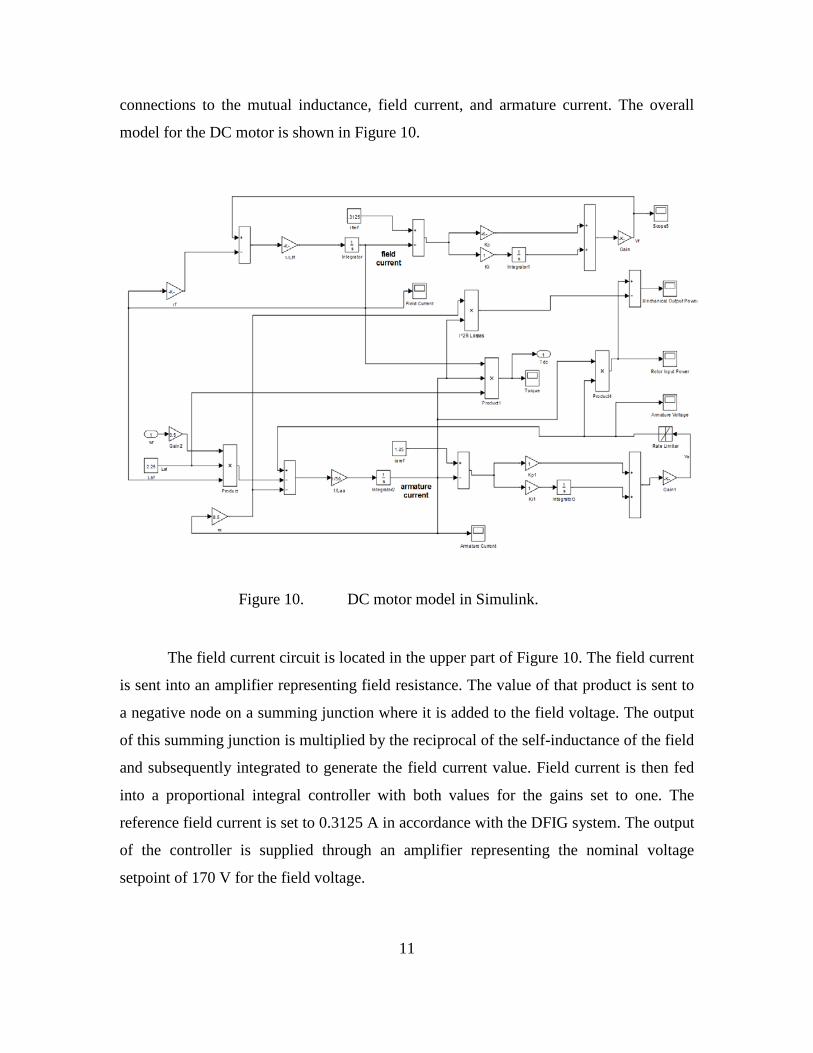
11

connections to the mutual inductance, field current, and armature current. The overall

model for the DC motor is shown in Figure 10.

Figure 10. DC motor model in Simulink.

The field current circuit is located in the upper part of Figure 10. The field current

is sent into an amplifier representing field resistance. The value of that product is sent to

a negative node on a summing junction where it is added to the field voltage. The output

of this summing junction is multiplied by the reciprocal of the self-inductance of the field

and subsequently integrated to generate the field current value. Field current is then fed

into a proportional integral controller with both values for the gains set to one. The

reference field current is set to 0.3125 A in accordance with the DFIG system. The output

of the controller is supplied through an amplifier representing the nominal voltage

setpoint of 170 V for the field voltage.

12

The armature current was designed in a manner similar to the field current circuit

and is located in the lower section of Figure 10. The product junction multiplies the field

current, the mutual inductance, and the rotor speed. That output is, in turn, subtracted

from the value of the armature voltage. The product of the armature resistance and the

armature current is also subtracted from armature voltage at the first summation junction.

The armature voltage is rate limited in order to prevent instantaneous changes in voltage.

This allows for more a more accurate behavioral model of rotor input power by allowing

for a delay reduction in power during the transient. The remainder of the circuit is

identical to the field current circuit with the exception of the value for the reference

armature current (1.25 A).

The machine output torque is calculated at the center of Figure 10 in accordance

with (2.2). The torque is defined as the variable dcT for the drawing.

The calculation for the armature electrical input power is located on the right edge

of Figure 10. The formula [5]

a ain iP v= (2.7)

is used to determine the input power into the rotor of the DC motor, where inP is

electrical input power to the DC motor armature. The armature losses are found from [5]

22

a ai r iP r= (2.8)

where 2i rP is defined as the armature losses. The armature losses are computed on

Figure 10 near the center of the diagram. Next, 2i rP is subtracted from inP to compute a

more realistic value for the machine output power that takes into account armature losses

for the DC motor. The resulting equation is

2out in i rP P P= − , (2.9)

where outP is the final computed mechanical output power for the simulation.

13

E. MODEL VALIDATION FOR ARMATURE AND FIELD CURRENTS

The armature and field currents were extracted as data from the operating

machinery. The measured values were then compared to the simulated values for

accuracy. This step was done to ensure that the simulation was commanding and

outputting the values expected before continuing on to more complex calculations.

Figure 11 is a plot of the measured and simulated armature and field currents during a

transition between 1,441 RPM and 1,981 RPM.

Figure 11. Measured and simulated armature and field currents.

The values of both simulated currents correspond well with the operational data.

The computation of armature current and field current was found to be accurate.

Parameters such as input power and machine speed were simulated with the

understanding that the currents were correctly modeled.

14

F. MODEL VALIDATION FOR SPEED

1. Comparison between Operational Data and Simulated Data

In order to validate the accuracy of the circuit model constructed in Simulink, data

from the DFIG system in the lab was taken. The system was operated using a specific

speed profile. The speed data was extracted from the system and subsequently

implemented into the Matlab code for the DFIG system [2] found in Appendix B. This

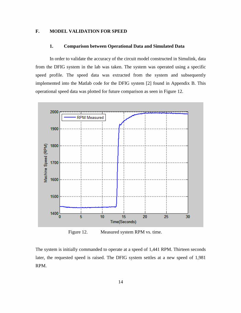
operational speed data was plotted for future comparison as seen in Figure 12.

Figure 12. Measured system RPM vs. time.

The system is initially commanded to operate at a speed of 1,441 RPM. Thirteen seconds

later, the requested speed is raised. The DFIG system settles at a new speed of 1,981

RPM.

15

The simulation was adjusted to reflect the magnitude and duration of the speeds in

the operational portion. The torque constant was removed from the simulation, and the

input torque to the DFIG was connected to the output of the DC motor model. The

overall model of the DFIG system, including the separately excited DC motor, is shown

in Appendix C. The simulation was executed and speed data was collected and plotted.

The plot of the simulated speed data for the test runs is displayed in Figure 13.

Figure 13. Simulated system RPM vs. time.

16

The measured data and the simulated data were plotted together on the same

graph to provide for easier analysis. This yielded the data pictured in Figure 14.

Figure 14. Measured and simulated system RPM vs. time.

2. Results

The data from the simulation compares very favorably with the operational speed.

The simulated system responds more rapidly to the change in speed; however, there is

little difference between the two operating sets at any point during the run.

The difference in response time is likely due to rapid response of the simulation

versus the actual machine. The model constructed in Simulink is an ideal machine.

17

While inertia is accounted for in the data measured in earlier experiments, not all losses

were accounted for. These particular components of the DC motor operation mute the

response when compared to an ideal system.

G. MODEL VALIDATION FOR ELECTRICAL INPUT POWER

1. Comparison between Operational Data and Simulated Data

The next step was validation of the simulation for the electrical input power to the

armature of the DC motor. Input power was measured for the DC motor armature while

operating the DFIG under the same conditions as the speed runs. The power, in watts,

versus the time, in seconds, was plotted on the graph shown in Figure 15.

Figure 15. Measured input power of DC motor vs. time.

18

The simulation was set to plot the output power data corresponding to the same

set of conditions. Figure 16 is a display of the power input to the rotor versus time for the

Simulink model. Both plots were placed on the same axes, found in Figure 17, for

comparative analysis.

Figure 16. Simulated input power of DC motor vs. time.

19

Figure 17. Measured and simulated input power vs. time.

2. Results

The simulated armature input power tracks well with the actual power profile

supplied to the armature of the DC motor. However, the simulation assumes ideal

characteristics. The change in speed causes a significant drop in input power (about 20%)

before the power rises to a new, higher level. This drop-off, while present in the

simulation, is not as pronounced. This is most likely caused by the simulation being able

to respond instantaneously to changes in operational parameters, whereas the actual

system cannot. The effect was produced in the simulation by adding a rate limiter at the

output of the armature voltage to mute the response. The rate limiter prevented the drop

in armature current from causing the voltage to surge to a higher value instantaneously.

During analysis, the armature self-inductance value in the simulation was lowered

to 30 H. The result was a more rapid response to the change in speed. This alteration

provided for a model that more accurately mimicked the machine behavior.

20

H. MODELING MECHANICAL OUTPUT POWER

After modeling the input power, attention was turned to creating an accurate

simulation of the mechanical output power. Finding the output power required a

theoretical approach due to the unavailability of the required equipment to measure the

torque at the rotor. Therefore, certain assumptions were made to estimate the value of the

output.

Windage and friction losses are present in any spinning machine [5]. However,

there was no way to directly measure these values. The losses for the DC machine were

considered to be limited to armature losses for this study. While not completely accurate,

the simulated output is a much more realistic value for machine output power than

assuming 100% efficiency between rotor input power and mechanical output power. The

plot of the modeled output power, in watts, versus time, in seconds, for the speed

transition between 1,441 and 1,981 RPM is found in Figure 18.

Figure 18. Simulated output power of DC motor.

21

The output power is noticeably lower than the armature input power in Figure 17 when

analyzing the same time period. Consideration of the armature losses causes this

reduction.

I. CHAPTER SUMMARY

In this chapter, the DC motor operational theory was reviewed. The theory of

operation was used as a basis to model a DC motor that was used as a torque input to a

DFIG system simulation. Data was gathered from the operational system and compared

to the simulation to determine whether system operation speed could be accurately

predicted. Experimentation showed that the emulated speed was consistent with actual

system operation.

The input power was also discussed. The resulting comparison found the

simulation to accurately model of the rotational output power during steady state

conditions. Transitions in speed caused disturbances in the input power that were not

fully accounted for by the model. Overall, the model matches the operation of the

machinery well. The next section uses this model to determine output power of the DC

motor based on operating speeds derived from wind patterns within a particular region.

22


23

III. MODELING WIND PROFILES

A. INTRODUCTION

Speed prediction has been shown to be accurate in our wind power emulator. The

motor emulator can now be used to model the wind profiles of different geographic

locations. The DC motor replaces the turbine and gearbox that act as the prime mover for

a commercial wind turbine. By mapping the wind speeds in an area to the particular RPM

of the DC machine, a particular wind profile of a region can be generated.

B. MAPPING STRATEGY FOR WIND SPEED TO DC MOTOR SPEED

1. Overview

The process of determining the mapping procedure for wind speed to DC motor

shaft RPM is covered in this section. The methodologies of assigning the numerical

values of speed to the machine as well as the selection of the geographic area are

discussed.

2. Geographic Area Selection

The geographic area was selected based on two factors. The first requirement was

that the area be of significance to the DoD. This was done to tailor the research toward

the goals of [1].

The second factor taken into consideration was the availability of wind speed data

for the area. There are several military installations located throughout the nation. Not all

of them have a significant amount of historical wind speed data readily available.

Viewing the problem from these two perspectives led to choosing Norfolk,

Virginia as the area of study. There is a large amount of data archived by the National

Climatic Data Center [6]. The data focused on for this study was the average wind speed.

The information was held by the National Climatic Data Center was compiled over a 54-

year period. The monthly and annual average wind speeds are present.

24

The monthly data from [6] is presented in Table 2. Average wind speed is given

in miles per hour (MPH).

Table 2. Monthly wind speed averages for Norfolk, Virginia, from [6].

Norfolk, Virginia

Month Average Wind Speed (MPH)

January 11.4

February 11.8

March 12.3

April 11.8

May 10.4

June 9.7

July 8.9

August 8.8

September 9.6

October 10.2

November 10.3

December 10.9

The maximum average wind speed, by month, occurs in March at 12.3 MPH. The

minimum average wind speed is 8.8 MPH in August. It was necessary to develop a

mapping scheme that was able to encompass all of these speeds.

3. Mapping Strategy

The machine speed for commercial wind turbines is varied according to the wind

speed. As a result, maximum power conversion is performed at all speeds. The ideal

25

machine speed for a particular turbine and gearbox combination follows a peak power

curve as a function of wind speed and turbine speed [2]. To simplify the model, the

curved was linearized.

It was decided to set the maximum motor speed equal to a wind speed of 13

MPH. The motor speed was then scaled for the average monthly wind speed

proportionally using

2000 RPM13 MPHo MRPM S= × (2.10)

where ORPM is the operating speed for the system in RPM and MS is the average

monthly wind speed in MPH. The results of the scaling are found in Table 3.

Table 3. Scaling of monthly average wind speed in Norfolk, Virginia, to motor RPM.

Month MS ORPM

January 11.4 1754 February 11.8 1815 March 12.3 1892 April 11.8 1815 May 10.4 1600 June 9.7 1492 July 8.9 1369

August 8.8 1354 September 9.6 1477

October 10.2 1569 November 10.3 1585 December 10.9 1677

The value of ORPM was rounded to the nearest whole number to facilitate easier

calculations. Information from this data set was used as part of the validation of the

simulation as a model for wind speed.

26

4. Simulation of Different Wind Speeds

The motor speeds derived from the mapping were input into the simulation to

replicate the different average wind speeds across each month in Norfolk. The associated

output power levels for the machine speeds were plotted. In Figure 19, ORPM is plotted

versus time for each month. The simulation speed begins at 1,754 RPM to represent the

month of January. Every four seconds, ORPM is shifted to that of each subsequent

month.

Figure 19. Simulated average DC motor speed by month for wind turbine in Norfolk.

5. Simulation of Output Power Based on Wind Speeds

The output power produced by the simulation was graphed in Figure 20.

27

Figure 20. Simulated average DC motor output power by month for Norfolk.

The changes in power are organized in the same manner as the changes in speed.

The power begins with the value corresponding to the month of January. The value of

ORPM is adjusted every four seconds according the month represented. This led to the

variations in power level seen in the plot. The steady state power at each change in speed

indicates the predicted output power of the machine for that speed.

6. Analysis of Simulated Speed and Power

The plots contained within this chapter illustrate the scenarios of speed and power

production. The correlation between the speed of operation and the mechanical output

power was proven through the data plots. Simulated monthly power was almost directly

proportional to the speed.

28

The plot of power does not instantly jump to the final value based on the speed.

This is due to the rate limiter installed in the circuit for the voltage. The behavioral traits

of the machine are shown on the graph and, therefore, it takes a finite amount of time to

reach a new output power. The transition time of four seconds allows the model to reach

a steady state value of power for the given speed before transitioning to the next value.

C. CHAPTER SUMMARY

In this chapter, a mapping strategy was devised for converting wind speed to

rotational speed of the DC motor. The simulation was run using the mapped speeds as a

basis for commanded speed changes. Output power of the machine was calculated based

on the simulated operating speeds.

The correlation between the rotational speed and mechanical output power of the

DC machine was proven. This model can now be adjusted for specific scenarios in

operational speed. Conclusions to the study and further research options are discussed in

the next chapter.

29

IV. CONCLUSIONS AND FUTURE RESEARCH

A. CONCLUSIONS

In this thesis, the theory behind the operation of DC motors was reviewed.

Understanding of this theory allowed for the creation of a Simulink model representing a

separately excited DC motor. Testing was completed to validate the model outputs of

speed and rotational power. Using wind speeds mapped to the RPM of the machine, we

showed how the output power of the DC motor varied with the speed of the machine.

B. FUTURE RESEARCH

The DC motor used can be modeled in greater detail. Slew rate limiting of the

applied armature voltage was added and improved the prediction of the simulation

compared to the measured results. The physics behind this behavioral model should be

explored further. This would allow for a more accurate profile of the machine that models

the responses more faithfully.

A separate study should also measure the output of the DFIG to compare against

the output of the DC motor. The relationship between the two should be detailed. The

theoretical output of a larger system, such as those used in wind turbines, can be scaled

from the data obtained.

Future work should also include matching the DC machine to specific wind

turbine blades and gearboxes. The output power in this thesis uses a linearized model to

convert wind speed to machine speed. For an actual wind turbine, the ideal operating

points are based on a curve [2]. By modeling the curve, behavior of a specific

combination of turbine blades and gearbox can be analyzed.

30


31

APPENDIX A

Lab-Volt DC Machine

This machine can be run independently as a DC motor or a DC generator. The armature,

shunt field, and series field windings are terminated separately on the faceplate to permit

long and short shunt as well as cumulatively and differentially compounded motor

and generator connections. This machine is fitted with exposed movable brushes to

allow students to study the effect of armature reaction and commutation while the

machine is operating under load. An independent, circuit-breaker protected, shunt-field

rheostat is mounted on the faceplate for motor speed control or generator output voltage

adjustment.

32

Model 8211 – DC Motor/Generator 120/208 V – 60 Hz 220/380 V – 50 Hz 240/415 V – 50 Hz

Power Requirement 120/208 V 220/380 V 240/415 V

Rating Motor Output Power

Generator Output Power

Armature Voltage

Shunt Field Voltage

Full Load Speed

Full Load Motor Current

Full Load Generator Current

175 W

120 W 110 W 120 W

120 V – DC 220 V – DC 240 V – DC

120 V – DC 220 V – DC 240 V – DC

1800 r/min 1500 r/min 1500 r/min

2.8 A 1.3 A 1.1 A

1 A 0.5 A 0.5 A

Physical Characteristics Dimensions (H x W x D)

Net Weight

308 x 291 x 440 mm (12.1 x 11.5 x 17.3 in)

14.1 kg (31 lb)

33

APPENDIX B

Simulink Model Files

Figure 21. Overall DFIG system, from [3].

34

Figure 22. Induction Machine of Overall DFIG system, from [3].

.j:::ds """' -.;_, I

I I I'"' ~· "' ~ G) - I "''

I L: ' ,.,

J:S,i_qs

h3 I""-"' rl [ "'' -+Lj-~'!' r-- - psi d;

idr1

fqsx ..... fdsx -

- ~~ ~ ..... y

I ~;s-"' ....... f~y -

~~· ,_ ..

--..c:D (,;:;:;-)""' psi_d' ""' ... _. r~=~·

rottonents.

~:-"" Te

l _n

~:-" T' <OlC<<XnlroUe< "'' .,._., ~ JE,i_nd ·u

~-l""'

iqs

I f- ""' Xls

ln4

.. _mq I f-- f- .n

J' t:o IS= ~

ids

·u ... L__

~- -·

I 1--- ltqsy ,_ ~

~

'--'--' .. L__

ltdsy ::

j.- i ..,.,.. j'Oi00 .,. -fb

rotacu.ents1 SlbsysE.m2 ~

<ota in

D fa

tn -G>-r- in'o'B'SE Kr

L-fu.'"""'-'" psi_~ r-

~L_ GBin2

""-"' '----

.-;:: ... ~ .., power in

-;:; h3Qu3 .... o.5

""'-""' Slbsy5iem 1 1n10ut1

'"" _J,,.o.a p;i_crO

Sub:.ystern3

35

Figure 23. Subsystem of Induction Machine, from [3].

Figure 24. Inverse Ks transformation in Subsystem, from [3].

36

Figure 25. Inverse Ks transformation1 in Subsystem, from [3].

37

Figure 26. Subsystem1 of Induction Machine, from [3].


38


Figure 29. Stator of Subsystem3, from [3].

39

Figure 30. Stator1 of Subsystem3, from [3].

Figure 31. Inverse Kr transformation of Induction Machine, from [3].

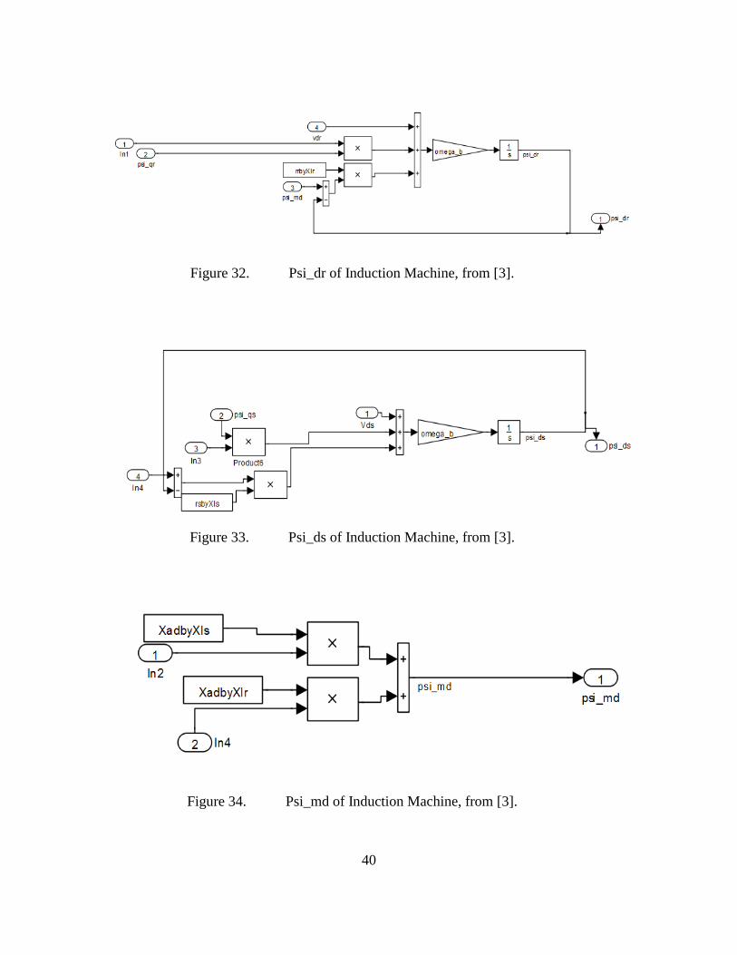
40

Figure 32. Psi_dr of Induction Machine, from [3].

Figure 33. Psi_ds of Induction Machine, from [3].

Figure 34. Psi_md of Induction Machine, from [3].

41

Figure 35. Psi_mq of Induction Machine, from [3].

Figure 36. Psi_qr of Induction Machine, from [3].

Figure 37. Psi_qs of Induction Machine, from [3].

42

Figure 38. Rotor controller of Induction Machine, from [3].

43

Figure 39. AC source of Rotor Controller, from [3].

Figure 40. Ks transformation of Rotor Controller, from [3].

44

Figure 41. Inverse trans of Rotor Controller, from [3].

Figure 42. Rotor currents of Induction Machine, from [3].

45

Figure 43. Rotor currents1 of Induction Machine, from [3].

Figure 44. Torque of Induction Machine, from [3].

46

Figure 45. Input torque of Overall DFIG system.

47

Figure 46. Separately excited DC motor of input torque.

48

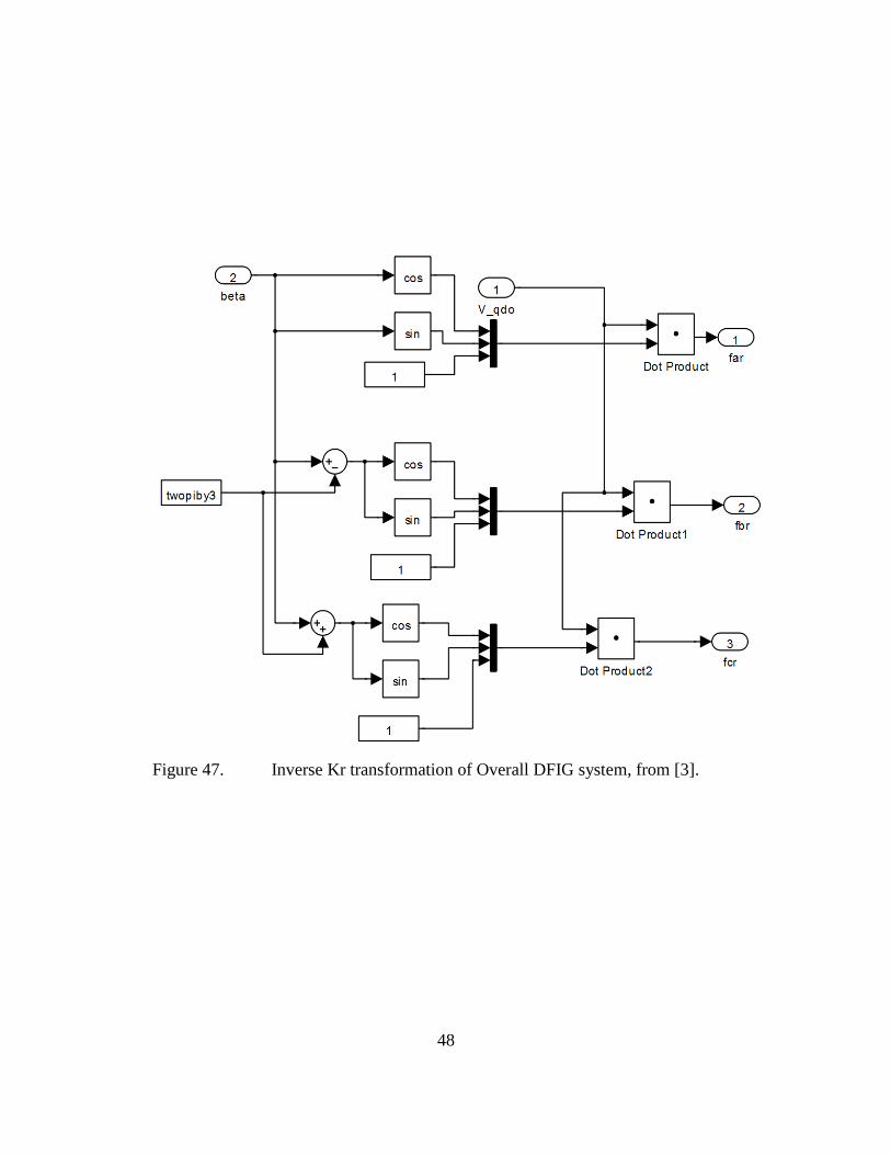
Figure 47. Inverse Kr transformation of Overall DFIG system, from [3].

49

Figure 48. Inverse Ks transformation of Overall DFIG system, from [3].

Figure 49. Torque equation of Overall DFIG system, from [3].

50


51

APPENDIX C

Matlab M-Files

Plot_recorder_update.m % Jonathan Hines Jan12 clear all; omega_b = 2*pi*60; %------------------------------------------------- omegar_ic = omega_b*0.8; %1441 RPM; used for initial tests omega2=omega_b*0.3; omega_jan=367; %used for monthly power data; replace in model omega_feb=0.035*omega_jan; omega_mar=0.044*omega_jan; omega_apr=-0.044*omega_jan; omega_may=-0.123*omega_jan; omega_jun=-0.062*omega_jan; omega_jul=-0.070*omega_jan; omega_aug=-0.009*omega_jan; omega_sep=0.070*omega_jan; omega_oct=0.052*omega_jan; omega_nov=0.009*omega_jan; omega_dec=0.052*omega_jan; sim asynchronous_gen_backupgio_hines_thesis; %connect input torque load data3; delay_time=-.0045-.0005; %load data3; %---------------------------------------------------------------------- %Plots figure(1); %Speed plot measured and simulated plot(timedataold',ch8_final,'b','linewidth',2); hold on; plot(speed_sim(:,1)-30,speed_sim(:,2),'g','linewidth',2) hold off; axis([0 30 1400 2000]); %title('Measured and Simulated Speed'); legend('RPM Measured','RPM Simulated', 'Location', 'NorthWest'); ylabel('Machine Speed (RPM)'); xlabel('Time(Seconds)'); grid; figure(2); % Input Power plot measured and simulated plot(ScopeData14(:,1)-30,ScopeData14(:,2),'g','linewidth',2);

52

hold on; plot(time_dc,dc_machine_power,'b','linewidth',2); hold off; axis ([0 30 110 220]); %title('Rotor Input Power of DC Motor'); legend('Simulated Input Power', 'Measured Input Power', 'Location','NorthWest'); ylabel('Input Power (Watts)'); xlabel('Time (Seconds)'); grid; %-------------------------------------------------------------------------- %Connect the monthly summation block in the induction machine model figure(3); %Monthly speed figure plot(speed_sim(:,1)-30,speed_sim(:,2),'g','linewidth',2) axis([0 48 1300 1900]); %title('Simulated Average DC Motor Speed Scaled by Monthly Norfolk Wind Speeds'); legend('RPM_O For Simulated Wind Speed', 'Location', 'NorthEast'); ylabel('Machine Speed (RPM)'); xlabel('Time(Seconds)'); grid; figure(4); %Monthly Power Figure plot(power_out(:,1)-30,power_out(:,2),'g','linewidth',2); axis ([0 48 110 180]); %title('Simulated Mechanical Output Power of DC Motor Scaled by Monthly Norfolk Winds Speeds'); legend('Output Power by Month for Norfolk', 'Location','NorthEast'); ylabel('Output Power (Watts)'); xlabel('Time (Seconds)'); grid; %-------------------------------------------------------------------------- plot_exp_data_newscope; figure(5); %Armature and Field Currents plot(ia_plot(:,1)-30,ia_plot(:,2), 'g', 'linewidth',4); %Simulated Ia hold on; plot(datavec_ch4(:,1)+13.8,ch4_smooth,'b'); %Measured Armature Current plot(if_plot(:,1)-30, if_plot(:,2), 'c', 'linewidth',4); %Simulated If plot(datavec(:,1)+13.8,ch2_smooth,'m'); %Measured Field Current hold off; axis([12.5 15 0.2 1.4]); %title('Simulated and Measured Armature and Field Currents'); legend('Simulated Armature Current', 'Measured Armature Current','Simulated Field Current', 'Measured Field Current', 'Location', 'East'); ylabel('Current (Amperes)'); xlabel('Time (Seconds)'); grid;

53

figure(6); %Output Power plot plot(power_out(:,1)-30,power_out(:,2),'g','linewidth',2); axis ([0 30 110 200]); %title('Simulated Mechanical Output Power of DC Motor'); legend('Simulated Output Power', 'Location','NorthWest'); ylabel('Output Power (Watts)'); xlabel('Time (Seconds)'); grid; figure(7); %Speed plot measured plot(timedataold',ch8_final,'b','linewidth',2); axis([0 30 1400 2000]); %title('Measured Speed'); legend('RPM Measured', 'Location', 'NorthWest'); ylabel('Machine Speed (RPM)'); xlabel('Time(Seconds)'); grid; figure(8); %Speed plot simulated plot(speed_sim(:,1)-30,speed_sim(:,2),'g','linewidth',2) axis([0 30 1400 2000]); %title('Simulated Speed'); legend('RPM Simulated', 'Location', 'NorthWest'); ylabel('Machine Speed (RPM)'); xlabel('Time(Seconds)'); grid; figure(9); % Input Power plot Simulated plot(ScopeData14(:,1)-30,ScopeData14(:,2),'g','linewidth',2); axis ([0 30 110 220]); %title('Simulated Rotor Input Power of DC Motor'); legend('Simulated Input Power', 'Location', 'NorthWest'); ylabel('Input Power (Watts)'); xlabel('Time (Seconds)'); grid; figure(10); % Input Power plot Measured plot(time_dc,dc_machine_power,'b','linewidth',2); axis ([0 30 110 220]); %title('Measured Rotor Input Power of DC Motor'); legend('Measured Input Power', 'Location', 'NorthWest'); ylabel('Input Power (Watts)'); xlabel('Time (Seconds)'); grid;

54

initial_vars_asynchronous_gen.m, from [3] %initial_vars_asynchronous_gen omega_b = 2*pi*60; % omega2=-omega_b*1/14; tstep=.0008; tstop=60; twopiby3 = 2*pi/3; poles = 4; polesby2J = poles/2/(2.04e-3*1.5); %Inertia from Nytko thesis Kpgain_speed=.033*2; Kigain_speed=.0033*4; Kpgain=15/2*10; % Divide by 2 becuae Vdc=60 is half of 120 in the FPGA program Kigain=2/2*40; %Parameters from Edwards thesis work for DFIG rs=12; rr = 4; Xls =9; Xm =180*0.6; % no load Xm =180*0.7; % with generation Xlr = 9+omega_b*400e-6; rsbyXls = rs/Xls; rrbyXlr = rr/Xlr; Xaq = 1/(1/Xm+1/Xls+1/Xlr); Xad = Xaq; XaqbyXls = Xaq/Xls; XaqbyXlr = Xaq/Xlr; XadbyXls = Xad/Xls; XadbyXlr = Xad/Xlr; V_phase = 220*sqrt(2)/sqrt(3); %Peak value used in Simulink for source model % omegar_ic = omega_b*13/14; psi_qsic=0; psi_dsic=0; psi_qric=0; psi_dric=0;

55

shift_time2.m from [3] %shift_time2 function [data]= shift_time2 (z15_LSB, z15_MSB, z16_LSB, z16_MSB, data_size) z15_new_LSB=uint8(zeros(data_size,1)); z15_new_MSB=uint8(zeros(data_size,1)); index=0; for ii=1:data_size if z15_MSB(ii)>=2^7 index=index+1; z15_new_MSB(ii)=z15_MSB(ii)-2^7; if z15_new_MSB(ii)>=2^6 index=index+1; z15_new_MSB(ii)=z15_new_MSB(ii)-2^6; end elseif z15_MSB(ii)>=2^6 z15_new_MSB(ii)=z15_MSB(ii)-2^6; else z15_new_MSB(ii)=z15_MSB(ii); end end index=0; for ii=1:data_size if z15_LSB(ii)>=2^7 index=index+1; z15_new_LSB(ii)=z15_LSB(ii)-2^7; if z15_new_LSB(ii)>=2^6 index=index+1; z15_new_LSB(ii)=z15_new_LSB(ii)-2^6; end elseif z15_LSB(ii)>=2^6 z15_new_LSB(ii)=z15_LSB(ii)-2^6; else z15_new_LSB(ii)=z15_LSB(ii); end end %channel 16 z16_new_LSB=uint8(zeros(data_size,1)); z16_new_MSB=uint8(zeros(data_size,1)); index=0; for ii=1:data_size if z16_MSB(ii)>=2^7 index=index+1; z16_new_MSB(ii)=z16_MSB(ii)-2^7; if z16_new_MSB(ii)>=2^6 index=index+1; z16_new_MSB(ii)=z16_new_MSB(ii)-2^6; end elseif z16_MSB(ii)>=2^6 z16_new_MSB(ii)=z16_MSB(ii)-2^6; else

56

z16_new_MSB(ii)=z16_MSB(ii); end end index=0; for ii=1:data_size if z16_LSB(ii)>=2^7 index=index+1; z16_new_LSB(ii)=z16_LSB(ii)-2^7; if z16_new_LSB(ii)>=2^6 index=index+1; z16_new_LSB(ii)=z16_new_LSB(ii)-2^6; end elseif z16_LSB(ii)>=2^6 z16_new_LSB(ii)=z16_LSB(ii)-2^6; else z16_new_LSB(ii)=z16_LSB(ii); end end data15=(double(z15_new_LSB)+double(z15_new_MSB)*2^6); data16=(double(z16_new_LSB)+double(z16_new_MSB)*2^6)*2^12; data=((data15+data16)-(data15(1)+data16(1)))*2^17/25e6;

57

shift2alj.m, from [3] %shift2alj function [data]= shiftb2 (z_LSB, z_MSB,data_size) z_new_LSB=uint8(zeros(data_size,1)); z_new_MSB=uint8(zeros(data_size,1)); index=0; for ii=1:data_size if z_MSB(ii)>=2^7 index=index+1; z_new_MSB(ii)=z_MSB(ii)-2^7; if z_new_MSB(ii)>=2^6 index=index+1; z_new_MSB(ii)=z_new_MSB(ii)-2^6; end elseif z_MSB(ii)>=2^6 z_new_MSB(ii)=z_MSB(ii)-2^6; else z_new_MSB(ii)=z_MSB(ii); end end index=0; for ii=1:data_size if z_LSB(ii)>=2^7 index=index+1; z_new_LSB(ii)=z_LSB(ii)-2^7; if z_new_LSB(ii)>=2^6 index=index+1; z_new_LSB(ii)=z_new_LSB(ii)-2^6; end elseif z_LSB(ii)>=2^6 z_new_LSB(ii)=z_LSB(ii)-2^6; else z_new_LSB(ii)=z_LSB(ii); end end for ii=1:data_size if z_new_MSB(ii) >= 2^5 data(ii)=(double(z_new_LSB(ii))+double(z_new_MSB(ii))*2^6-double(2^12)); else data(ii)=(double(z_new_LSB(ii))+double(z_new_MSB(ii))*2^6); end end

58

plot_exp_data_newscope.m, from [3] % EC3150 - Laboratory - G.Oriti, Jul '09 % This file acquires the data vector from the oscilloscope % and plots it versus time % It also plots the spectrum of the input data vector using the fft data_in=xlsread('Tek_CH2_Wfm.csv'); data_in_ch3=xlsread('Tek_CH3_Wfm.csv'); data_in_ch4=xlsread('Tek_CH4_Wfm.csv'); len = length(data_in); datavec=data_in(15:len,1:2); datavec_ch3=data_in_ch3(15:len,1:2); datavec_ch4=data_in_ch4(15:len,1:2); ch2_smooth=(datavec(:,2)+[datavec(2:len-14,2);0])/2; ch3_smooth=(datavec_ch3(:,2)+[datavec_ch3(2:len-14,2);0])/2; ch4_smooth=(datavec_ch4(:,2)+[datavec_ch4(2:len-14,2);0])/2; figure(1); % plot(datavec(:,1),datavec(:,2),'b:'); plot(datavec(:,1),ch2_smooth,'m'); hold on; % plot(datavec_ch3(:,1),datavec_ch3(:,2)/10-15,'g'); % plot(datavec_ch4(:,1),datavec_ch4(:,2),'r'); %plot(datavec_ch3(:,1),ch3_smooth/10-15,'k'); plot(datavec_ch4(:,1),ch4_smooth,'b'); hold off; title('DC Machine measurements during step change in speed'); xlabel('time [s]'); grid on legend('I_f_i_e_l_d','I_a','Location','NorthEast'); axis([-1 1 0 4]);

59

Data_crunching.m from [3] %data_crunching %post-processing and plotting data %processing channel 1 data z_LSB1a=z(:,1); z_MSB1a=z(:,2); z_LSB1b=z(:,1+32); z_MSB1b=z(:,2+32); z_LSB1c=z(:,1+32+32); z_MSB1c=z(:,2+32+32); z_LSB1d=z(:,1+32+32+32); z_MSB1d=z(:,2+32+32+32); z_LSB1e=z(:,1+16); z_MSB1e=z(:,2+16); z_LSB1f=z(:,1+32+16); z_MSB1f=z(:,2+32+16); z_LSB1g=z(:,1+32+32+16); z_MSB1g=z(:,2+32+32+16); z_LSB1h=z(:,1+32+32+32+16); z_MSB1h=z(:,2+32+32+32+16); for ii=1:totalpoints/2 z_LSB1(8*ii-7) =z_LSB1a(ii); z_LSB1(8*ii-6) =z_LSB1e(ii); z_LSB1(8*ii-5) =z_LSB1b(ii); z_LSB1(8*ii-4) =z_LSB1f(ii); z_LSB1(8*ii-3) =z_LSB1c(ii); z_LSB1(8*ii-2) =z_LSB1g(ii); z_LSB1(8*ii-1) =z_LSB1d(ii); z_LSB1(8*ii) =z_LSB1h(ii); z_MSB1(8*ii-7) =z_MSB1a(ii); z_MSB1(8*ii-6) =z_MSB1e(ii); z_MSB1(8*ii-5) =z_MSB1b(ii); z_MSB1(8*ii-4) =z_MSB1f(ii); z_MSB1(8*ii-3) =z_MSB1c(ii); z_MSB1(8*ii-2) =z_MSB1g(ii); z_MSB1(8*ii-1) =z_MSB1d(ii); z_MSB1(8*ii) =z_MSB1h(ii); end ch1_data= shiftb2alj (z_LSB1, z_MSB1, totalpoints*4); ch1_final=ch1_data/2^2; %processing channel 4 data gain1=1/(1/3000+1/200000)/(1/(1/3000+1/200000)+56000*2)*1.05; z_LSB4a=z(:,7); z_MSB4a=z(:,8); z_LSB4b=z(:,7+32); z_MSB4b=z(:,8+32); z_LSB4c=z(:,7+32+32); z_MSB4c=z(:,8+32+32);

60

z_LSB4d=z(:,7+32+32+32); z_MSB4d=z(:,8+32+32+32); z_LSB4e=z(:,7+16); z_MSB4e=z(:,8+16); z_LSB4f=z(:,7+32+16); z_MSB4f=z(:,8+32+16); z_LSB4g=z(:,7+32+32+16); z_MSB4g=z(:,8+32+32+16); z_LSB4h=z(:,7+32+32+32+16); z_MSB4h=z(:,8+32+32+32+16); for ii=1:totalpoints/2 z_LSB4(8*ii-7) =z_LSB4a(ii); z_LSB4(8*ii-6) =z_LSB4e(ii); z_LSB4(8*ii-5) =z_LSB4b(ii); z_LSB4(8*ii-4) =z_LSB4f(ii); z_LSB4(8*ii-3) =z_LSB4c(ii); z_LSB4(8*ii-2) =z_LSB4g(ii); z_LSB4(8*ii-1) =z_LSB4d(ii); z_LSB4(8*ii) =z_LSB4h(ii); z_MSB4(8*ii-7) =z_MSB4a(ii); z_MSB4(8*ii-6) =z_MSB4e(ii); z_MSB4(8*ii-5) =z_MSB4b(ii); z_MSB4(8*ii-4) =z_MSB4f(ii); z_MSB4(8*ii-3) =z_MSB4c(ii); z_MSB4(8*ii-2) =z_MSB4g(ii); z_MSB4(8*ii-1) =z_MSB4d(ii); z_MSB4(8*ii) =z_MSB4h(ii); end ch4_data= shiftb2alj (z_LSB4, z_MSB4, totalpoints*4); ch4_final=ch4_data/2^2; %processing channel 5 data z_LSB5a=z(:,9); z_MSB5a=z(:,10); z_LSB5b=z(:,9+32); z_MSB5b=z(:,10+32); z_LSB5c=z(:,9+32+32); z_MSB5c=z(:,10+32+32); z_LSB5d=z(:,9+32+32+32); z_MSB5d=z(:,10+32+32+32); z_LSB5e=z(:,9+16); z_MSB5e=z(:,10+16); z_LSB5f=z(:,9+32+16); z_MSB5f=z(:,10+32+16); z_LSB5g=z(:,9+32+32+16); z_MSB5g=z(:,10+32+32+16); z_LSB5h=z(:,9+32+32+32+16); z_MSB5h=z(:,10+32+32+32+16); for ii=1:totalpoints/2 z_LSB5(8*ii-7) =z_LSB5a(ii); z_LSB5(8*ii-6) =z_LSB5e(ii); z_LSB5(8*ii-5) =z_LSB5b(ii); z_LSB5(8*ii-4) =z_LSB5f(ii);

61

z_LSB5(8*ii-3) =z_LSB5c(ii); z_LSB5(8*ii-2) =z_LSB5g(ii); z_LSB5(8*ii-1) =z_LSB5d(ii); z_LSB5(8*ii) =z_LSB5h(ii); z_MSB5(8*ii-7) =z_MSB5a(ii); z_MSB5(8*ii-6) =z_MSB5e(ii); z_MSB5(8*ii-5) =z_MSB5b(ii); z_MSB5(8*ii-4) =z_MSB5f(ii); z_MSB5(8*ii-3) =z_MSB5c(ii); z_MSB5(8*ii-2) =z_MSB5g(ii); z_MSB5(8*ii-1) =z_MSB5d(ii); z_MSB5(8*ii) =z_MSB5h(ii); end ch5_data= shiftb2alj (z_LSB5, z_MSB5, totalpoints*4); ch5_final=ch5_data/2^2; %processing channel 6 data gain2=1/(1/6800+1/200000)/(1/(1/6800+1/200000)+120000*2)*1.05; %DC sensor gain gainI=3/1000*330; %current sensor gain z_LSB6a=z(:,11); z_MSB6a=z(:,12); z_LSB6b=z(:,11+32); z_MSB6b=z(:,12+32); z_LSB6c=z(:,11+32+32); z_MSB6c=z(:,12+32+32); z_LSB6d=z(:,11+32+32+32); z_MSB6d=z(:,12+32+32+32); z_LSB6e=z(:,11+16); z_MSB6e=z(:,12+16); z_LSB6f=z(:,11+32+16); z_MSB6f=z(:,12+32+16); z_LSB6g=z(:,11+32+32+16); z_MSB6g=z(:,12+32+32+16); z_LSB6h=z(:,11+32+32+32+16); z_MSB6h=z(:,12+32+32+32+16); for ii=1:totalpoints/2 z_LSB6(8*ii-7) =z_LSB6a(ii); z_LSB6(8*ii-6) =z_LSB6e(ii); z_LSB6(8*ii-5) =z_LSB6b(ii); z_LSB6(8*ii-4) =z_LSB6f(ii); z_LSB6(8*ii-3) =z_LSB6c(ii); z_LSB6(8*ii-2) =z_LSB6g(ii); z_LSB6(8*ii-1) =z_LSB6d(ii); z_LSB6(8*ii) =z_LSB6h(ii); z_MSB6(8*ii-7) =z_MSB6a(ii); z_MSB6(8*ii-6) =z_MSB6e(ii); z_MSB6(8*ii-5) =z_MSB6b(ii); z_MSB6(8*ii-4) =z_MSB6f(ii); z_MSB6(8*ii-3) =z_MSB6c(ii); z_MSB6(8*ii-2) =z_MSB6g(ii); z_MSB6(8*ii-1) =z_MSB6d(ii); z_MSB6(8*ii) =z_MSB6h(ii); end ch6_data= shiftb2alj (z_LSB6, z_MSB6, totalpoints*4);

62

ch6_final=ch6_data/2^6; %processing channel 7 data z_LSB7a=z(:,13); z_MSB7a=z(:,14); z_LSB7b=z(:,13+32); z_MSB7b=z(:,14+32); z_LSB7c=z(:,13+32+32); z_MSB7c=z(:,14+32+32); z_LSB7d=z(:,13+32+32+32); z_MSB7d=z(:,14+32+32+32); z_LSB7e=z(:,13+16); z_MSB7e=z(:,14+16); z_LSB7f=z(:,13+32+16); z_MSB7f=z(:,14+32+16); z_LSB7g=z(:,13+32+32+16); z_MSB7g=z(:,14+32+32+16); z_LSB7h=z(:,13+32+32+32+16); z_MSB7h=z(:,14+32+32+32+16); for ii=1:totalpoints/2 z_LSB7(8*ii-7) =z_LSB7a(ii); z_LSB7(8*ii-6) =z_LSB7e(ii); z_LSB7(8*ii-5) =z_LSB7b(ii); z_LSB7(8*ii-4) =z_LSB7f(ii); z_LSB7(8*ii-3) =z_LSB7c(ii); z_LSB7(8*ii-2) =z_LSB7g(ii); z_LSB7(8*ii-1) =z_LSB7d(ii); z_LSB7(8*ii) =z_LSB7h(ii); z_MSB7(8*ii-7) =z_MSB7a(ii); z_MSB7(8*ii-6) =z_MSB7e(ii); z_MSB7(8*ii-5) =z_MSB7b(ii); z_MSB7(8*ii-4) =z_MSB7f(ii); z_MSB7(8*ii-3) =z_MSB7c(ii); z_MSB7(8*ii-2) =z_MSB7g(ii); z_MSB7(8*ii-1) =z_MSB7d(ii); z_MSB7(8*ii) =z_MSB7h(ii); end ch7_data= shiftb2alj (z_LSB7, z_MSB7, totalpoints*4); ch7_final=ch7_data/2^6; %processing channel 8 data z_LSB8a=z(:,15); z_MSB8a=z(:,16); z_LSB8b=z(:,15+32); z_MSB8b=z(:,16+32); z_LSB8c=z(:,15+32+32); z_MSB8c=z(:,16+32+32); z_LSB8d=z(:,15+32+32+32); z_MSB8d=z(:,16+32+32+32); z_LSB8e=z(:,15+16); z_MSB8e=z(:,16+16); z_LSB8f=z(:,15+32+16); z_MSB8f=z(:,16+32+16); z_LSB8g=z(:,15+32+32+16); z_MSB8g=z(:,16+32+32+16);

63

z_LSB8h=z(:,15+32+32+32+16); z_MSB8h=z(:,16+32+32+32+16); for ii=1:totalpoints/2 z_LSB8(8*ii-7) =z_LSB8a(ii); z_LSB8(8*ii-6) =z_LSB8e(ii); z_LSB8(8*ii-5) =z_LSB8b(ii); z_LSB8(8*ii-4) =z_LSB8f(ii); z_LSB8(8*ii-3) =z_LSB8c(ii); z_LSB8(8*ii-2) =z_LSB8g(ii); z_LSB8(8*ii-1) =z_LSB8d(ii); z_LSB8(8*ii) =z_LSB8h(ii); z_MSB8(8*ii-7) =z_MSB8a(ii); z_MSB8(8*ii-6) =z_MSB8e(ii); z_MSB8(8*ii-5) =z_MSB8b(ii); z_MSB8(8*ii-4) =z_MSB8f(ii); z_MSB8(8*ii-3) =z_MSB8c(ii); z_MSB8(8*ii-2) =z_MSB8g(ii); z_MSB8(8*ii-1) =z_MSB8d(ii); z_MSB8(8*ii) =z_MSB8h(ii); end ch8_data= shiftb2alj (z_LSB8, z_MSB8, totalpoints*4); ch8_final=ch8_data; %processing channel 2 and 3 data to create time vector %processing channel 2 data z_LSB2a=z(:,3); z_MSB2a=z(:,4); z_LSB2b=z(:,3+32); z_MSB2b=z(:,4+32); z_LSB2c=z(:,3+32+32); z_MSB2c=z(:,4+32+32); z_LSB2d=z(:,3+32+32+32); z_MSB2d=z(:,4+32+32+32); z_LSB2e=z(:,3+16); z_MSB2e=z(:,4+16); z_LSB2f=z(:,3+32+16); z_MSB2f=z(:,4+32+16); z_LSB2g=z(:,3+32+32+16); z_MSB2g=z(:,4+32+32+16); z_LSB2h=z(:,3+32+32+32+16); z_MSB2h=z(:,4+32+32+32+16); for ii=1:totalpoints/2 z_LSB2(8*ii-7) =z_LSB2a(ii); z_LSB2(8*ii-6) =z_LSB2e(ii); z_LSB2(8*ii-5) =z_LSB2b(ii); z_LSB2(8*ii-4) =z_LSB2f(ii); z_LSB2(8*ii-3) =z_LSB2c(ii); z_LSB2(8*ii-2) =z_LSB2g(ii); z_LSB2(8*ii-1) =z_LSB2d(ii); z_LSB2(8*ii) =z_LSB2h(ii); z_MSB2(8*ii-7) =z_MSB2a(ii); z_MSB2(8*ii-6) =z_MSB2e(ii);

64

z_MSB2(8*ii-5) =z_MSB2b(ii); z_MSB2(8*ii-4) =z_MSB2f(ii); z_MSB2(8*ii-3) =z_MSB2c(ii); z_MSB2(8*ii-2) =z_MSB2g(ii); z_MSB2(8*ii-1) =z_MSB2d(ii); z_MSB2(8*ii) =z_MSB2h(ii); end %processing channel 3 data z_LSB3a=z(:,5); z_MSB3a=z(:,6); z_LSB3b=z(:,5+32); z_MSB3b=z(:,6+32); z_LSB3c=z(:,5+32+32); z_MSB3c=z(:,6+32+32); z_LSB3d=z(:,5+32+32+32); z_MSB3d=z(:,6+32+32+32); z_LSB3e=z(:,5+16); z_MSB3e=z(:,6+16); z_LSB3f=z(:,5+32+16); z_MSB3f=z(:,6+32+16); z_LSB3g=z(:,5+32+32+16); z_MSB3g=z(:,6+32+32+16); z_LSB3h=z(:,5+32+32+32+16); z_MSB3h=z(:,6+32+32+32+16); for ii=1:totalpoints/2 z_LSB3(8*ii-7) =z_LSB3a(ii); z_LSB3(8*ii-6) =z_LSB3e(ii); z_LSB3(8*ii-5) =z_LSB3b(ii); z_LSB3(8*ii-4) =z_LSB3f(ii); z_LSB3(8*ii-3) =z_LSB3c(ii); z_LSB3(8*ii-2) =z_LSB3g(ii); z_LSB3(8*ii-1) =z_LSB3d(ii); z_LSB3(8*ii) =z_LSB3h(ii); z_MSB3(8*ii-7) =z_MSB3a(ii); z_MSB3(8*ii-6) =z_MSB3e(ii); z_MSB3(8*ii-5) =z_MSB3b(ii); z_MSB3(8*ii-4) =z_MSB3f(ii); z_MSB3(8*ii-3) =z_MSB3c(ii); z_MSB3(8*ii-2) =z_MSB3g(ii); z_MSB3(8*ii-1) =z_MSB3d(ii); z_MSB3(8*ii) =z_MSB3h(ii); end timedataold= shift_time2 (z_LSB2, z_MSB2, z_LSB3, z_MSB3, totalpoints*4);

timedata=[0:(2^11-1)]/25e6*2^12;

65

LIST OF REFERENCES

[1] “Defense infrastructure: Department of Defense renewable energy initiatives,” Briefing for the Committees on Armed Services, United States Senate and House of Representatives. Government Accountability Office, 26 April 2010.

[2] S. Muller, M. Deicke, and R. W. de Doncker. “Doubly fed induction generator systems for wind turbines.” IEEE Industry Applications Magazine, pp. 26–33, May/June 2002.

[3] A. L. Julian and G. Oriti. Class notes for EC4130, Advanced Electrical Machinery Systems and Work on DFIG, Naval Postgraduate School, 2007–2012 (unpublished).

[4] J. R. Derges, “Torque control of a separate-winding excitation DC motor for a dynamometer,” M.S. thesis, Naval Postgraduate School, 2010.

[5] P. C. Krause, O. Wasynczuk, and S. D. Sudhoff, Analysis of Electric Machinery and Drive Systems. Hoboken, NJ: John Wiley & Sons, 2002.

[6] Dan Dellinger. “Wind- average wind speed- (MPH), ” August 20, 2008 [Online]. Available: http://lwf.ncdc.noaa.gov/oa/climate/online/ccd/avgwind.html

66


67

INITIAL DISTRIBUTION LIST

1. Defense Technical Information Center Ft. Belvoir, Virginia 2. Dudley Knox Library Naval Postgraduate School Monterey, California 3. Dr. R. Clark Robertson Navy Postgraduate School Monterey, California 4. Dr. Alexander L. Julian Navy Postgraduate School Monterey, California 5. Dr. Giovanna Oriti Navy Postgraduate School Monterey, California 6. LT Jonathan T. Hines, USN NAVSUBSCOL New London Groton, Connecticut

Documents

NAVAL POSTGRADUATE SCHOOL · The separately excited DC motor was investigated to develop the equations necessary to produce the model. Once the required equations were understood,