NAVAL POSTGRADUATE SCHOOL - oc.nps.educhu/web_paper/thesis/wheatley.pdf · naval postgraduate school monterey, california ... mine warfare: investigation of bedforms, waves, tides,

NAVAL

POSTGRADUATE SCHOOL

MONTEREY, CALIFORNIA

THESIS

Approved for public release; distribution is unlimited

DETERMINING ROUTE SURVEY PERIODICITY FOR MINE WARFARE: INVESTIGATION OF BEDFORMS,

WAVES, TIDES, AND CURRENTS

by

Nicola S. Wheatley

September 2009

Thesis Advisor: Peter Chu Second Reader: Thomas H. C. Herbers

THIS PAGE INTENTIONALLY LEFT BLANK

i

REPORT DOCUMENTATION PAGE Form Approved OMB No. 0704-0188Public reporting burden for this collection of information is estimated to average 1 hour per response, including the time for reviewing instruction, searching existing data sources, gathering and maintaining the data needed, and completing and reviewing the collection of information. Send comments regarding this burden estimate or any other aspect of this collection of information, including suggestions for reducing this burden, to Washington headquarters Services, Directorate for Information Operations and Reports, 1215 Jefferson Davis Highway, Suite 1204, Arlington, VA 22202-4302, and to the Office of Management and Budget, Paperwork Reduction Project (0704-0188) Washington DC 20503. 1. AGENCY USE ONLY (Leave blank)

2. REPORT DATE September 2009

3. REPORT TYPE AND DATES COVERED Master’s Thesis

4. TITLE AND SUBTITLE Determining Route Survey Periodicity for Mine Warfare: Investigation of Bedforms, Waves, Tides, and Currents

5. FUNDING NUMBERSN6230609PO00123

6. AUTHOR(S) Nicola S. Wheatley 7. PERFORMING ORGANIZATION NAME(S) AND ADDRESS(ES)

Naval Postgraduate School Monterey, CA 93943-5000

8. PERFORMING ORGANIZATION REPORT NUMBER

9. SPONSORING /MONITORING AGENCY NAME(S) AND ADDRESS(ES)Ronald E. Betsch, Naval Oceanographic Office 1002 Balch Blvd, Stennis Space Center, MS 39529

10. SPONSORING/MONITORING AGENCY REPORT NUMBER

11. SUPPLEMENTARY NOTES The views expressed in this thesis are those of the author and do not reflect the official policy or position of the Department of Defense or the U.S. Government. 12a. DISTRIBUTION / AVAILABILITY STATEMENT Approved for public release; distribution is unlimited

12b. DISTRIBUTION CODE

13. ABSTRACT (maximum 200 words) To retain maritime security, an up to date database of mine countermeasures route surveys is essential. In 2005, the United Kingdom Hydrographic Office (UKHO) developed a GIS weighted suitability model to determine survey periodicity; allowing optimization of survey resources, increasing time and cost efficiency. The US currently has no such model. Bedforms are an integral part of the survey periodicity problem. Sediment grain size, tides, currents, and wind-generated waves are influential in bedform formation. In this thesis, San Francisco Bay was chosen as a case study. To investigate if sediment properties change over time, localized grab samples for a three-year period were analyzed. The analysis showed little variability in sediment characteristics at a given location. A weighted suitability model based on the UKHO model was constructed. Three layers were developed including sediment grain size, interpolated from 174 grab samples, tidal and current data from over 50 current stations and ripple height inferred from wind generated wave height. A weighting for each layer was determined. Regions indicating the presence of bedforms were assigned a low survey periodicity, as bedforms reduced, survey periodicity was increased. High-resolution multi-beam survey data was used as a comparison and validation, this showed extremely good correlation with the model.

14. SUBJECT TERMS Mine Warfare, Route Survey, Bedforms, Waves, Tides, Currents, Survey Periodicity, Sediment Transport, Sediment Dynamics, Bathymetry, GIS, Weighted Suitability Model, San Francisco Bay

15. NUMBER OF PAGES

124 16. PRICE CODE

17. SECURITY CLASSIFICATION OF REPORT

Unclassified

18. SECURITY CLASSIFICATION OF THIS PAGE

Unclassified

19. SECURITY CLASSIFICATION OF ABSTRACT

Unclassified

20. LIMITATION OF ABSTRACT

UU NSN 7540-01-280-5500 Standard Form 298 (Rev. 8-98) Prescribed by ANSI Std. Z39.18

ii


iii

Approved for public release; distribution is unlimited

DETERMINING ROUTE SURVEY PERIODICITY FOR MINE WARFARE: INVESTIGATION OF BEDFORMS, WAVES, TIDES, AND CURRENTS

Nicola S. Wheatley

Lieutenant, Royal Navy BSc (Hons), University of Plymouth, 2000

Submitted in partial fulfillment of the requirements for the degree of

MASTER OF SCIENCE IN PHYSICAL OCEANOGRAPHY

from the

NAVAL POSTGRADUATE SCHOOL September 2009

Author: Nicola S. Wheatley

Approved by: Peter Chu Thesis Advisor

Thomas H. C. Herbers Second Reader

Jeffrey D. Paduan Chairman, Department of Oceanography

iv


v

ABSTRACT

To retain maritime security, an up-to-date database of mine

countermeasures route surveys is essential. In 2005, the United Kingdom

Hydrographic Office (UKHO) developed a GIS weighted suitability model to

determine survey periodicity; allowing optimization of survey resources,

increasing time and cost efficiency. The U.S. currently has no such model.

Bedforms are an integral part of the survey periodicity problem. Sediment grain

size, tides, currents, and wind-generated waves are influential in bedform

formation. In this thesis, San Francisco Bay was chosen as a case study. To

investigate if sediment properties change over time, localized grab samples for a

three-year period were analyzed. The analysis showed little variability in

sediment characteristics at a given location. A weighted suitability model based

on the UKHO model was constructed. Three layers were developed including

sediment grain size, interpolated from 174 grab samples, tidal and current data

from over 50 current stations and ripple height inferred from wind generated

wave height. A weighting for each layer was determined. Regions indicating the

presence of bedforms were assigned a low survey periodicity, as bedforms

reduced, survey periodicity was increased. High-resolution multi-beam survey

data was used as a comparison and validation, this showed extremely good

correlation with the model.

vi


vii

TABLE OF CONTENTS

I. INTRODUCTION ............................................................................................. 1 A. AIMS AND OBJECTIVES .................................................................... 1 B. MINE WARFARE ................................................................................. 2

1. The Threat ................................................................................ 2 2. Mine Classification .................................................................. 3

a. Bottom Mines ................................................................ 3 b. Moored Mines ................................................................ 3 c. Drifting Mines ................................................................ 3

3. Mine Warfare Operations ........................................................ 4 a. Mining ............................................................................ 4 b. Mine Counter-Measures (MCM) ................................... 4

4. Environmental Factors for Mine Warfare ............................... 4 a. Bathymetry .................................................................... 6 b. Tides and Currents ....................................................... 7 c. Seabed Sediment Type and Sedimentation ................ 8

C. THE UKHO MODEL ........................................................................... 10 1. The UKHO Model Concepts .................................................. 10

a. The Mine Counter Measures Environment ............... 10 b. The Maritime Environment ......................................... 10 c. GIS Modeling ............................................................... 11

2. Model Interpretation .............................................................. 13 3. Model Limitations .................................................................. 14

D. OVERVIEW OF THIS STUDY ............................................................ 14

II. SEDIMENT DYNAMICS AND BEDFORM EVOLUTION .............................. 17 A. SEDIMENT TRANSPORT .................................................................. 17

1. Sediment Type ....................................................................... 18 a. The Wentworth Scale .................................................. 19 b. NAVOCEANO Database Data. .................................... 20

2. Grain Size Distribution and Fluid Flow ................................ 21 3. Threshold of Sediment Movement ....................................... 23

B. BEDFORM FORMATION ................................................................... 25 1. Ripples .................................................................................... 27 2. Dunes ...................................................................................... 27 3. Antidunes ............................................................................... 27

C. INFLUENCE OF CURRENTS AND WAVES ON BEDFORMS ......... 27 1. Currents .................................................................................. 28 2. Waves ..................................................................................... 30 3. Combined Current and Wave Interaction ............................ 31

D. MODELING WAVE GENERATED RIPPLES ..................................... 32

III. CASE STUDY: SAN FRANCISCO BAY ....................................................... 39 A. INTRODUCTION ................................................................................ 39

viii

B. SEDIMENT ANALYSIS: COMPARISON OF LOCALIZED SAMPLE DATA AND DATABASE DATA ......................................... 40 1. Data and Methods .................................................................. 40

a. Sediment Sample Collection ...................................... 41 b. Sediment Sample Analysis. ....................................... 41 c. Localized Sample Data. .............................................. 43

2. Results and Analysis ............................................................. 44 a. Localized Sample Data Comparison. ........................ 44 b. Comparison of Ripple Heights ................................... 50 c. NAVOCEANO Database Comparison. ....................... 53 d. Accuracy and Errors. .................................................. 54

C. USGS MULTI-BEAM SURVEY DATA ............................................... 55 1. Bed Patterns in San Francisco Bay ..................................... 56 2. Temporal Variation in Bedform Morphology ....................... 59 3. Bedform Asymmetry and Sediment Transport Patterns .... 64

IV. DETERMINING ROUTE SURVEY PERIODICITY FOR SAN FRANCISCO BAY .............................................................................................................. 67 A. INTRODUCTION ................................................................................ 67 B. THE MODELING CONCEPT ............................................................. 67

1. The Input Layers .................................................................... 68 a. Predicted Bedform Type ............................................. 68 b. Predicted Bottom Currents ........................................ 71 c. Predicted Wave Generated Ripple Heights ............... 76

2. Layer Classification ............................................................... 78 a. Predicted Bedform Type ............................................. 79 b. Predicted Bottom Currents ........................................ 80 c. Predicted Wave Generated Ripple Heights ............... 82

C. ASSIGNING LAYER WEIGHTING..................................................... 84 1. Option 1 .................................................................................. 85 2. Option 2 .................................................................................. 87 3. Option 3 .................................................................................. 88 4. Option 4 .................................................................................. 89 5. Option 5 .................................................................................. 90

D. DETERMINING SURVEY PERIODICITY ........................................... 91

V. CONCLUSIONS AND RECOMMENDATIONS ............................................. 93 A. SUMMARY OF RESULTS ................................................................. 94

1. Localized Sample Data and Database Comparison Results .................................................................................... 94

2. USGS Multi-beam Survey Results ........................................ 94 3. Modeling Results ................................................................... 95

B. RECOMMENDATIONS ...................................................................... 96 1. Recommendations for the UKHO Model .............................. 97 2. Limitations .............................................................................. 97 3. Recommendations for Further Study .................................. 98

ix

LIST OF REFERENCES ........................................................................................ 100

INITIAL DISTRIBUTION LIST ............................................................................... 104

x


xi

LIST OF FIGURES

Figure 1. The Mine Warfare Environment (After National Research Council,

2000) .................................................................................................... 5 Figure 2. GIS Weighted Suitability Model (From Armishaw, 2005) .................... 11 Figure 3. Relationship between model parameters, showing the weightings

assigned to each layer (From Armishaw, 2005) ................................. 13 Figure 4. Sediment process triad (From Proudman, 2009) ................................ 18 Figure 5. Settling velocities of grains in water at 20oC as a function of grain

diameter and shape factor (From Komar and Reimers, 1978). .......... 23 Figure 6. Forces acting on a grain resting on the seabed (From Liu, 2001) ...... 24 Figure 7. Shields diagram showing the threshold of suspension (From Dyre,

1986) .................................................................................................. 25 Figure 8. Flow over Ripples, Dunes and Antidunes (From Liu, 2001) ............... 26 Figure 9. Bedform prediction diagram (From Liu, 2001) .................................... 26 Figure 10. Typical bedforms in order of increased stream power (From

Deigaard, 1992) .................................................................................. 28 Figure 11. Relationship between total bed shear stress and flow velocity for

different bedforms (From Deigaard, 1992) ......................................... 29 Figure 12. A) Bedform shape in oscillatory flow, B) Bedform shape in steady

flow (From Deigaard, 1992) ................................................................ 29 Figure 13. Sketch of vortices formed over a vortex ripple (From Deigaard,

1992) .................................................................................................. 30 Figure 14. Horizontal velocity profile and water particle orbit as predicted by

linear wave theory (From Liu, 2001) ................................................... 31 Figure 15. Comparison of current and wave velocity profiles (From Liu, 2001) ... 32 Figure 16. Differences in near bottom orbital velocity for different wave heights

and wave periods, for a sediment size of 2.5phi, results obtained using the Wiberg and Harris model .................................................... 36

Figure 17. Differences in wave generated ripple heights for different wave periods and sediment size, for a wave with a height of 1 m, results obtained using the Wiberg and Harris model ...................................... 37

Figure 18. Van Veen grab on board R/V Point Sur. ............................................. 41 Figure 19. Locations of the localized samples used for comparison. ................... 43 Figure 20. Column Graphs for positions A–D, showing sample breakdown, per

year, from largest grain size (left) to smallest grain size (right) .......... 47 Figure 21. Sample mass (%) v’s grain size (mm) for positions A to D. Error

Bars indicate the 95% Confidence Interval in both dimensions. ......... 49 Figure 22. Positions A–D, overlaid on the NAVOCEANO HFEVA Dataset. ........ 53 Figure 23. Bedforms in the inlet throat of San Francisco Bay (With Permission,

from Barnard et al., 2007) ................................................................... 57 Figure 24. Bedforms inside San Francisco Bay (With Permission, from

Barnard et al., 2007) ........................................................................... 58

xii

Figure 25. A) Location of sand wave transects. B) Transect from mouth of San Francisco Bay. C) Transect in vicinity of Alcatraz Shoals. (With permission, from Barnard et al., 2007) ...................................... 61

Figure 26. Region of study between Alcatraz and Angel Island (With permission, from Barnard et al., In Press, 2009). ............................... 62

Figure 27. Transects from Figure 26. A) Transect A-B. B) Transect C-D. (With permission, from Barnard et al., In Press, 2009). ...................... 63

Figure 28. Complex current patterns offshore of Ocean Beach (with permission, from Barnard et al., 2007). .............................................. 64

Figure 29. Asymmetry values across the Golden Gate (with permission from Barnard et al., 2007). .......................................................................... 65

Figure 30. Inferred net bedload sediment transport directions based on asymmetry values, arrows indicated direction only, not magnitude (with permission, from Barnard et al., 2007). ...................................... 66

Figure 31. Flow chart showing the three layers used to predict survey periodicity. .......................................................................................... 68

Figure 32. Sediment type calculated from grab samples, locations of the grab samples are overlaid. ......................................................................... 69

Figure 33. Potential bedform areas. .................................................................... 70 Figure 34. Tidal Zones in the San Francisco Bay region. .................................... 71 Figure 35. Tidal Curves in the San Francisco Bay Region .................................. 72 Figure 36. The locations of the current station data used. ................................... 73 Figure 37. Surface currents, arrows indicate the magnitude and direction of

the current, red indicates ebb currents, green indicates flood currents. ............................................................................................. 74

Figure 38. Bottom currents, arrows indicate the magnitude and direction of the current, red indicates ebb currents, green indicates flood currents. Graduated depth scale shown in meters. ........................................... 74

Figure 39. Ebb and flood dominated regions, surface currents (left), bottom currents (right). ................................................................................... 75

Figure 40. Mean wave generated ripple heights in cm, for January (left) and July (right). .......................................................................................... 77

Figure 41. Predicted wave generated ripple height layer. .................................... 78 Figure 42. Weighted sediment size layer. ............................................................ 80 Figure 43. Weighted bottom currents layer. ......................................................... 82 Figure 44. Weighted wave generated ripple layer. .............................................. 84 Figure 45. Combined weighted layers, Option 1. ................................................. 86 Figure 46. Combined weighted layers, Option 2. ................................................. 87 Figure 47. Combined weighted layers, Option 3. ................................................. 88 Figure 48. Combined weighted layers, Option 4. ................................................. 89 Figure 49. Combined weighted layers, Option 5. ................................................. 90 Figure 50. Recommended survey periodicity for San Francisco Bay. ................. 92

xiii

LIST OF TABLES

Table 1. Impact Matrix of Oceanographic Factors, red – high importance, yellow – moderate importance, green – low importance. ...................... 6

Table 2. Data included in the UKHO model (From Armishaw, 2005) ............... 11 Table 3. Recommended re-survey intervals (From Armishaw, 2005) ............... 13 Table 4. The Wentworth Scale. (From Dyre, 1986) ......................................... 19 Table 5. NAVOCEANO HFEVA database sediment classification. (From

NAVOCEANO, 2003) ......................................................................... 21 Table 6. Mode of transport related to Rouse numbers (From Wikipedia,

2009) .................................................................................................. 22 Table 7. Sediment Classification based on Phi values for Positions A–D. ....... 44 Table 8. Ripple Characteristics for positions A–D. ........................................... 52 Table 9. 2009 sediments samples compared to NAVOCEANO Database

Data. ................................................................................................... 53 Table 10. Climatological data used in this study. ................................................ 76 Table 11. Weighting scheme for sediment size. ................................................. 79 Table 12. Weighting scheme for bottom currents. .............................................. 81 Table 13. Weighting scheme for wave generated ripples. .................................. 83

xiv

LIST OF ACRONYMS

BGS British Geological Survey

CEFAS Centre for Environment, Fisheries and Aquaculture Sciences

DW Deep Water

GEODB Geological Database

GIS Geographical Information Systems

HFEVA High Frequency Environmental Acoustics

MCM Mining and Mine Countermeasures

MODIS Moderate-Resolution Imaging Spectroradiometer

MS Microsoft

NASA National Aeronautics and Space Administration

NOAA National Oceanographic and Atmospheric Association

NAVOCEANO Naval Oceanographic Office

NPS Naval Postgraduate School

RSDB Route Survey Database

SEAs Strategic Environmental Assessments

UK United Kingdom

UKHO United Kingdom Hydrographic Office

US United States

USGS United States Geological Survey

VSW Very Shallow Water

xv

LIST OF SYMBOLS

ω Angular frequency

bτ Bed shear stress

α Coefficient to modify friction velocity

*cU Critical friction velocity

cθ Critical Shields parameter

CD Drag coefficient

d Diameter of a sediment particle

ρ Fluid density

DF Flow drag force

*U Friction velocity

X Grain size in mm

ϕ Grain size measurement

Xϕ Grain size mean

mϕ Grain size mean multiplied by percentage of sub-sample

ϕσ Grain size standard deviation

3ϕα Grain size skewness

g Gravity

CL Lift coefficient

D Mean grain diameter (mm)

0d Near bed orbital diameter

orbU Near bed orbital velocity

rH Ripple height

rL Ripple length

xvi

anoλ Ripple wavelength (anorbital)

orbλ Ripple wavelength (orbital)

subλ Ripple wavelength (suborbital)

oR Rouse Number

sρ Sediment density

sw Settling velocity

sU Shear velocity

θ Shields parameter

V Velocity

ν Viscosity of a fluid

κ Von Karman constant

h Water depth

H Wave height

k Wave number

T Wave period

c Wave speed

xvii

ACKNOWLEDGMENTS

I would like to thank my advisor, Prof. Peter Chu and second reader Prof.

Thomas Herbers for their support, advice and patience throughout this project.

For help during my practical work, thanks must go to Prof. Curt Collins and the

staff of the R/V Point Sur.

Many thanks to Dr. Julie Armishaw, from UKHO, for allowing me to

investigate her model and answering the many questions I asked at the

beginning of this project. Thanks also to Dr. Partrick Barnard, from USGS for

allowing me to use his data, ask questions, and provide comments and feedback

throughout the modeling process.

Lastly and most importantly, I would like to thank my family and friends

back in the UK and in Monterey for their continued support and encouragement

throughout my time at NPS.

xviii


1

I. INTRODUCTION

A. AIMS AND OBJECTIVES

In recent years the Navy has undergone a shift in operational focus from

the traditional ‘blue water operations’ in deep open ocean, to ‘brown water

operations’ in the littoral zone. The littoral, traditionally an unfamiliar area for

Naval operations, brings with it different challenges. A significant threat when

operating in the littoral are mines. Mine warfare is not a new concept; mines have

been used since the American Revolution. They are inexpensive, simple to

manufacture, and relatively easy to obtain and maintain. Mines have resulted in

damage and have sunk more ships in the past century than all other weapons

combined. More than 50 countries possess a mine-laying capability (National

Research Council, 2001).

Mines are used to deny sea control, in order to maintain war-fighting

capability, and naval forces need the ability to open and maintain sea lines of

communication in order to dominate the littoral battle space (Royal Navy, 2004).

In order to retain maritime security, it is essential to maintain an up-to-date

database of mine countermeasures route surveys, particularly for ports, harbors,

and sea-lanes of strategic importance.

The littoral region is subject to many temporal and spatial variations, and it

is therefore difficult to assess how often a region should be surveyed in order to

maintain up-to-date data. The United Kingdom Hydrographic Office (UKHO) has

developed a model to maintain the UK mine warfare route survey database,

taking into account environmental and geospatial parameters. This enables

survey periodicity to be calculated in order to optimize survey resources, thus

making this task more time and cost effective. The U.S. Navy currently has no

such model.

2

B. MINE WARFARE

1. The Threat

The first floating mine was designed by David Bushnell in 1776—‘the

Bushnell Keg’—it was used during the American Revolution. It was a primitive

design that was comprised of a watertight keg filled with gunpowder and a

flintlock detonator, which was suspended from a float. These mines were placed

in the Delaware River so that they would float into British ships that were

stationed down river (Royal Navy, 2009) (U.S. Navy and Marine Corp, 2005).

During the Second World War many different types of mine were

developed, new ways to lay the mines were also developed. Aircraft dropped

mines proved very successful; on average the Allies lost one mine-laying plane

for every twenty enemy ships sunk (Royal Navy, 2009).

In the Korean War, a major U.S. amphibious operation was delayed by

eight days due to a relatively primitive mine threat. The Admiral in charge of the

operation, Real Admiral Allan Smith was quoted as saying (Royal Navy, 2009):

A backward nation with a fleet of sampans designed at the time of Christ has used mines designed during the United States Civil War to halt the mightiest naval power in the history of the world’

This remains true today. The most recent use of mines in combat was

during the 1991 Gulf War. The Iraqi forces laid minefields, comprised of an

estimated 1300 mines (Royal Navy, 2009) (U.S. Navy and Marine Corp, 2005).

This resulted in two U.S. ships, the USS Princeton and the USS Tripoli, being

badly damaged.

The mine has played an important role in all major naval campaigns.

Although mines have become far more sophisticated, they remain relatively

cheap to manufacture and deploy. The cost of producing and laying a mine is

approximately 0.5% to 10% of the cost of removing it, and it can take up to two

hundred times longer to clear a mine field than to lay one (Wikipedia, 2009).

3

Mine damage to a ship can include hull rupture, caused by the pressure

wave created by detonation. Internal damage to equipment is caused by

vibration and flooding and also structural damage to the ship. The magnitude

and type of damage depends upon the size of the explosive force and the shock

resistance of the target (U.S. Navy and Marine Corps, 2005).

2. Mine Classification

Mine warfare is defined as the strategic and tactical use of sea mines and

their countermeasures (U.S. Navy and Marine Corps, 2005). Mines can be

classified into the following three categories.

a. Bottom Mines

Bottom mines, also known as Ground mines, are designed to sink

and rest on the seabed; they are most effective in comparatively shallow waters.

In deep waters, surface vessels may pass over the mine without triggering it. A

bottom mine planted in deep water is still effective against submarines. Acoustic,

magnetic, or pressure sensors can activate bottom mines.

b. Moored Mines

Moored Mines are placed at a pre-determined depth under water,

designed for deep-water, and are effective against submarines and surface

ships. The explosive charge and firing mechanism in a moored mine floats, and a

cable attached to an anchor on the bottom holds the case at the pre-determined

depth below the surface.

c. Drifting Mines

Drifting mines, which were banned under the Hague Convention of

1907, move freely through the water at or near the surface; they have no

anchoring devices. A moored mine that has lost its tether cable becomes a

drifting mine.

4

3. Mine Warfare Operations

Mine Warfare operations can be divided into two categories, Mining

and Mine Countermeasures (MCM).

a. Mining

Mining operations are used to establish or maintain control of sea

areas that are deemed to have tactical or significant importance. Mining has the

advantage of being able to inflict major damage on enemy shipping. A mine field

is covert and passive. This makes it an effective weapon in the denial of a sea

area to enemy forces. However, due to the passive nature of the mine, it cannot

distinguish between friendly or enemy forces. Two important concepts are:

Offensive Denial, which is the prevention of mining, and Defensive Protection,

which is reducing the risk of mines that have already been laid (Royal Navy,

2004).

b. Mine Counter-Measures (MCM)

MCM operations can be sub-divided into two categories. Offensive

MCM is the prevention of mines being laid in the first place. Strategic bombing of

enemy mine factories, depots, airfields, harbors, etc., can achieve this. Sinking

or shooting down of mine laying platforms, or excluding enemy mine layers from

areas of operations, can also achieve this. If enemy mines have already been

laid, then Defensive MCM operations must occur. These include active MCM

such as Mine-sweeping, Mine-hunting, and Clearance Diving.

4. Environmental Factors for Mine Warfare

For successful MCM operations, a number of factors must be taken into

account. The type, size, and aspect of the mine is important, as are the

environmental factors that will influence the behavior of the mine, and the

environmental factors that are present in the locality of the mine will influence

operations.

5

Mining is most likely to occur in the littoral region, where choke points and

shipping lanes are prime targets. In mine warfare the littoral region is divided into

four zones.

Figure 1. The Mine Warfare Environment (After National Research Council, 2000)

The Surf Zone: 0-3 m is where you find obstacles, anti invasion mines,

bottom, moored, and drifting mines. Very Shallow Water (VSW): 3-12 m is a

prime area for bottom, moored, and drifting mines. Shallow Water (SW): 12-60

m, likely mines include moored, drifting, and also rising mines, which are initially

deployed on the sea bed, and will be activated by either a time delay, pressure,

acoustic, or magnetic fluctuation that will cause the mine to rise. Bottom mines

can also be found in this region, but are deemed less effective than if laid in

VSW. Deep Water (DW): >60 m, moored, rising or drifting mines are likely,

bottom mines are unlikely to be laid at this depth.

The different environmental parameters in each zone have varying levels

of importance in MCM operations. They can be categorized by levels of

importance (National Research Council, 2000), these are summarized in Table 1.

6

The oceanographic factors that are considered to be of high importance in a

certain zone are assigned red, those of intermediate or moderate importance are

yellow, and those considered less important are green.

Surf Zone VSW SW DW

Bathymetry

Sediment Size

Seafloor Clutter

Bottom Roughness

Mine Burial

Currents/Waves

Water Clarity

Temperature and Salinity

Acoustic Properties N/A

Table 1. Impact Matrix of Oceanographic Factors, red – high importance, yellow – moderate importance, green – low importance.

The factors deemed more important in relation to survey periodicity are

discussed below.

a. Bathymetry

Bathymetry is an important factor when surveying the periodicity

problem. Spatial and temporal variations in water depth and seafloor profile can

influence the location and height of breaking waves, the position and strength of

surface currents, and the propagation of the tide into very shallow waters.

In the surf zone, temporal changes in bathymetry can influence

local dynamics in time periods as short as one day. In deeper waters, the

fractional changes are smaller and slower, but can still easily be sufficient to

cause mine burial. Prior knowledge of these conditions is an important aid to

operational planning (National Research Council, 2000). Bathymetry is important

7

in mine hunting operations due to scour or burial and bottom clutter

characteristics. Bathymetry measurements are more complex in shallow water,

the fluid dynamics mechanisms involved are increasingly sensitive to small-scale

features (National Research Council, 2000). Temporal changes are important,

modern survey techniques such as multi-beam surveys are increasingly being

used to study this area.

Burial potential varies strongly in the fluid environment with activity

generally increasing with decreasing depth (National Research Council, 2000).

In the deep and shallow water zone, burial can occur either when the mine is laid

or soon afterwards. Bathymetry in very shallow waters changes rapidly due to a

wide spectrum of bedforms, these are also found in shallow water. In this

dynamic morphology environment mines can quickly be susceptible to scour and

be buried. Little is known about the climatology, variability, and importance of

small-scale bedforms in shallow waters (National Research Council, 2000). It is

thought that bedforms are likely to be an important mechanism for mine burial.

Bedforms also affect the flow of the fluid through bottom dissipation. In bedform

regions mine detection is more difficult due to clutter. Knowledge of the presence

and persistence of low-clutter regimes (no bedforms) would be useful (National


b. Tides and Currents

Tidally driven changes of sea surface elevation vary globally from

negligible to several meters in very shallow waters. In the shallow and deep-

water zones, these elevation changes have little effect on mine hunting

operations or effectiveness. Tidal effects primarily influence mine warfare

operations in very shallow water and the surf zone, although in the surf zone tidal

currents are usually negligible compared to wave-driven flows (National


Tidal currents can cause an increase in the scour of bottom mines,

and can also cause significant transport of drifting mines. Outside the surf zone,

8

tidal currents are often greater than 0.5 m/s, this has a detrimental effect on diver

and marine mammal operations.

Currents can affect operations, safety, and potentially scour. There

is generally a decrease in magnitude of currents with depth. Deep and shallow

water flows are geostrophic and low-frequency (and are likely to be predictable),

while very shallow water and surf zone currents are more likely to be directly

forced through wind, wave-driving forces, or buoyancy fluxes due to runoff or

river outflow (National Research Council, 2000).

c. Seabed Sediment Type and Sedimentation

In the littoral zone, it is vital to have a good indication of sediment

type and seafloor characteristics if mine warfare operations are to be successful.

The physical, chemical, and magnetic properties of the seabed can be important

in all aspects of the mine warfare problem, for example (National Research

Council, 2000):

• Mine burial probability is a function of sediment properties; it is a

key factor for mine sweeping or hunting tactical decisions.

• Seafloor conductivity and water depth are key factors for

determining magnetic sweep paths.

• Bottom reflectivity is a factor in airborne LIDAR performance.

• Bottom sediment characteristics are a key factor in sediment

transport, which affects water clarity and mine burial.

With increased understanding of sediment types and properties,

many aspects of mine warfare operations can be improved and ultimately will

become more efficient. Mine burial is an extremely important factor in mine

warfare operations. There are four mechanisms by which mines will bury (U.S.

Navy and Marine Corps, 2005):

• Scour (current-induced and wave-induced)

9

• Migrating sand ridges

• Burial by deposition

• Impact burial

In order to be more effective, we need to have an increased

understanding of the forces that will cause mine burial (for example waves,

currents, and sediment transport). In particular, we need to understand how

these forces will interact with different mine types and the magnitude of these

forces.

Mines have various shapes and sizes. For example, a common

mine, called Manta, is a shallow seabed influence mine, which operates in

depths from 2.5 m to 100 m. It is designed to rest on the seabed even in a

region of strong flows. Typical dimensions of a Manta are: length 980 mm, width

980 mm, and height 470 mm. The dimensions are comparable to mines that

operate in similar depths; the Rockan has a length of 1015 mm, width 800 mm

and a height of just 385 mm. The Mk67 SLMM is 4090 mm in length, 485 mm in

width and 485 mm height. If sediment transport causes a change of

approximately 0.3 to 0.5 m in height of the seabed, it is significant in the possible

burial of mines—this is before factors such as scour are taken into account.

Significant work has been done in sediment transport research, and

a strong understanding of the physics involved has been developed, but these

efforts have been generic rather than mine warfare specific. For example; since

2001, strategic environmental assessments (SEAs) have been carried out in the

UK. They are managed by the Department of Trade and Industry, primarily

aimed at providing information for decisions that could affect the way large-scale

commercial energy resources are developed. However, due to the nature of the

research and the results obtained, this is an ideal source of data for the mine

warfare problem.

10

C. THE UKHO MODEL

The UKHO developed a weighted suitability Geographical Information

Systems (GIS) model in order to review the UK Mine Countermeasures Route

Survey maintenance schedule. The objective of the model is to optimize

resources, by determining which routes are susceptible to change and should be

surveyed at a higher frequency than those that are unlikely to change frequently

over time. This enables a more scientific approach to survey periodicity than that

of frequently re-surveying routes of higher strategic importance and surveying

lower priority routes on a less frequent basis.

1. The UKHO Model Concepts

There are three underlying concepts included in the UKHO model, which

are detailed in the following sections.

a. The Mine Counter Measures Environment

The Mine Counter Measures Environment focuses on factors that

are considered significant in mine burial, including burial mechanisms, burial

probability, and burial rate. These factors were used to estimate how a mine

could be buried, how likely this is, and the time period that these processes are

likely to take.

b. The Maritime Environment

The Maritime environment is an extremely important factor in

determining the survey periodicity for route surveys. The UKHO model included

seabed sediment types, sediment deposition, bottom texture, gas presence and

vessel traffic. A summary of the data included is shown in Table 2. The data

was obtained from many different sources, bottom texture and bottom contacts

data was taken from the UKHO Route Survey Database (RSDB) and processed

in Microsoft Excel, allowing it to be imported easily into ArcGIS. The British

Geological Survey (BGS) supplied the seabed sediment type data in a digital

11

map. In order to determine total suspended matter, satellite data from the NASA

MODIS satellites were used. The density of fishing vessels was obtained from

the Centre for Environment, Fisheries and Aquaculture Sciences (CEFAS). Gas

presence was taken from the UKHO Geological Database (GEODB) and vessel

traffic was supplied by NAVOCEANO.

Table 2. Data included in the UKHO model (From Armishaw, 2005)

c. GIS Modeling

In order to determine the survey periodicity, a weighted suitability

model was developed. This concept was used to simplify an extremely complex

problem.

Figure 2. GIS Weighted Suitability Model (From Armishaw, 2005)

In the UKHO model, each layer was re-classified to a scale of 0 to

9, with 0 representing a high degree of expected change and 9 representing little

change. Each layer was then assigned a weighting value that represented the

12

assessed importance of that layer. Each layer value was then multiplied with the

weighting value and added together for a particular location so that an

assessment could be made to the re-survey interval routes. The weighting

values used are shown in Figure 3. The route survey maintenance schedule was

determined using the three layers: Burial Probability, given a weighting of 0.40,

Burial Mechanisms, given a weighting of 0.40, and Change in Number of Bottom

Contacts, given a weighting of 0.20. Each can be considered a sub-model.

The Burial Probability sub-model is comprised of bottom texture,

weighting 0.30, seabed sediment type, weighting 0.30, total suspended

sediment, weighting 0.10, fishing activity, weighting 0.20 and gas presence,

weighting 0.10. The weightings in the sub-model represent the predicted

importance of each factor within that sub-model.

The Burial Mechanism sub-model is comprised of bottom texture,

weighting 0.45, seabed sediment type, weighting 0.45, and gas presence,

weighting 0.10. All three of these parameters were also included in the Burial

Probability sub-model, so it can be deduced that they are important in both

processes. The importance of bottom texture and seabed sediment type are

particularly relevant.

The Change in number of Bottom Contacts sub-model has two

input factors. The existing contact density has a weighting of 0.35. Additional

contacts from vessels, has a weighting of 0.65, this factor was devised by a

further sub-model including merchant vessels and fishing vessels, both of which

had a weighting of 0.50. The overall weighting of this sub-model is substantially

lower than the other two, indicating it has a lower importance on the overall route

survey maintenance schedule.

13

Figure 3. Relationship between model parameters, showing the weightings assigned to each layer (From Armishaw, 2005)

2. Model Interpretation

The model results were reclassified into four categories in order to assign

survey periodicity, and the results were then further sub-divided in two priority

groupings. The first, Priority 1, being areas of higher importance and the second,

Priority 2, being areas of lower importance. The categories are shown in Table

3, each category corresponds to a seabed changeability, with two recommended

survey intervals, depending on the priority of the region in question.

Category Seabed Changeability Priority 1 Survey Interval Priority 2 Survey Interval

1 HIGH 3-5 yrs 10-12 yrs 2 MODERATE-HIGH 5-7 yrs 12-15 yrs 3 LOW-MODERATE 7-10 yrs 15-20 yrs 4 LOW 10-15 yrs 20 yrs

Table 3. Recommended re-survey intervals (From Armishaw, 2005)

14

The model output layer was then re-plotted into the assigned seabed

changeability categories shown in Table 3, and from this a MCM Route survey-

planning matrix was constructed for UK route surveys.

3. Model Limitations

Recommendations for areas of further study from the UKHO 2005 report

included:

• Investigate the potential for the UKHO model to be used in other

geographic locations.

• Determine if any additional environmental factors should be

included in the model to refine the results.

The current iteration of the UKHO model is limited by the environmental

parameters that have not yet been included. Important factors such as waves,

tides and currents were not included.

The data included in the UKHO model, provides a good assessment for

survey periodicity in the UK region. It cannot be used in other geographical

locations due to the geographical boundaries of the input data. However, it could

be used as a basis for route re-survey models in other regions. The quantity and

quality of the data used to develop the UKHO model is extensive. Similar data

for other geographical locations, has proved difficult to source, and due to time

constraints of this study, a replica of the model for a different geographical

location has not been achieved.

D. OVERVIEW OF THIS STUDY

The primary goal of this research is to determine the variability of temporal

and spatial factors that will affect the survey periodicity of route surveys for Mine

Warfare. Many of these factors have been addressed and included in the UKHO

model. However, a significant omission is that of waves, tides, and currents.

Waves, tides, and currents have a huge impact on sediment transport and

15

bedform formation, which in turn will have a large impact on mine burial.

Therefore, these parameters are important in determining survey periodicity for

route surveys.

In this study, sediment transport and bedform evolution are reviewed. San

Francisco Bay is used as a case study. Experimental results from localized

sediment grabs are used to determine changes in sediment type with time, and

compared to the NAVOCEANO HFEVA sediment database. This allows the

validity of the database to be assessed. The effect of waves, tides, and currents

in the region are assessed. Theses results are then compared to multi-beam

data gathered by the United States Geological Survey (USGS), collected to

determine bedform evolution. The results from these two investigations are

analyzed and an assessment for mine warfare survey periodicity for this region is

determined.

From the San Francisco Bay results, the potential for additional layers

including waves, tides, and currents for the inclusion in the UKHO model are

reviewed and their values assessed.

16


17

II. SEDIMENT DYNAMICS AND BEDFORM EVOLUTION

A. SEDIMENT TRANSPORT

Sediment transport is the movement of sediment; it is typically due to the

gravity acting upon the sediment and the motion of the fluid in which the

sediment is located. It is complex, however, it is an extremely important factor in

determining the survey periodicity for route surveys. The sediment type will

influence the probability of a mine burial. The sediment transport rate has a

significant effect on the time period in which a mine will be buried or remain

uncovered, and thus detected during a survey.

Sediment transport is dependent on a number of variables, which include:

sediment size, shape and density of grains, settling velocity, sediment

availability, flow depth, water density and viscosity, bed shear stress, bedform

wavelength, height and steepness, maximum and residual tidal velocity and

wave period and amplitude (Dyre, 1986).

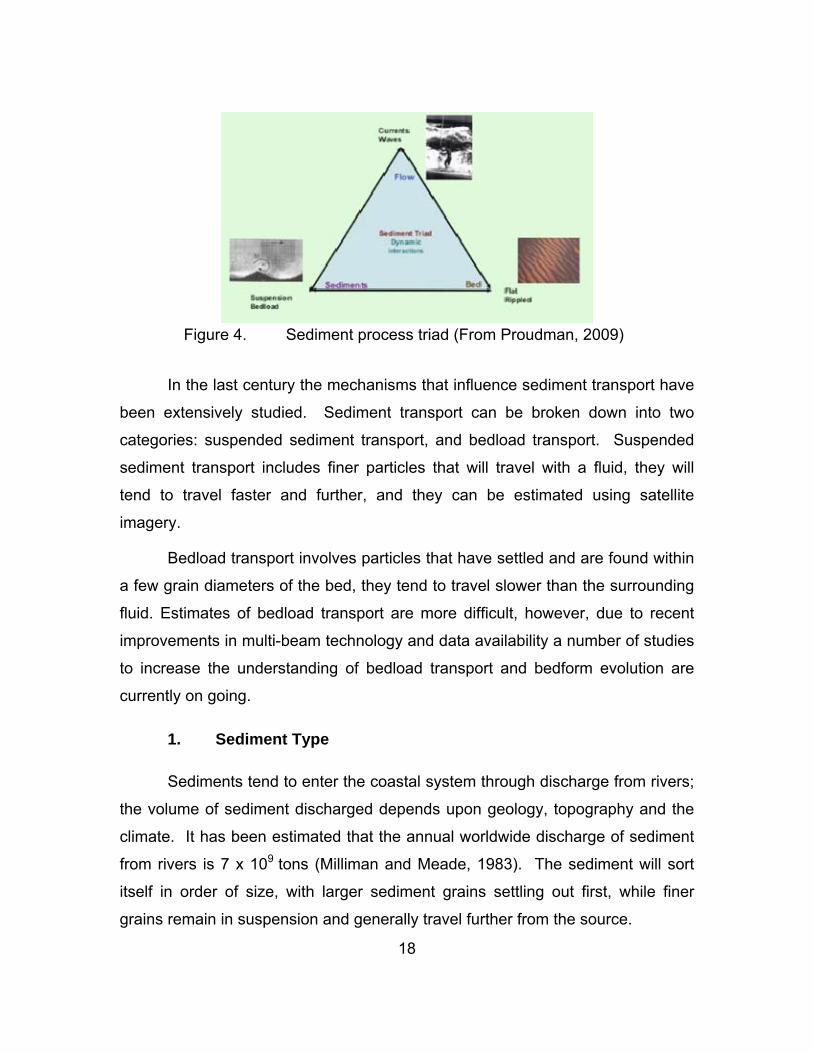
Figure 4 shows a schematic of the dynamic interactions of sediment

behavior. It shows a triad of three important factors: the sediment transport

mechanisms—for example if the sediment will be transported in suspension or as

bedload—, the type of seabed, and the flow that influences the sediment in the

form of waves and currents.

18

Figure 4. Sediment process triad (From Proudman, 2009)

In the last century the mechanisms that influence sediment transport have

been extensively studied. Sediment transport can be broken down into two

categories: suspended sediment transport, and bedload transport. Suspended

sediment transport includes finer particles that will travel with a fluid, they will

tend to travel faster and further, and they can be estimated using satellite

imagery.

Bedload transport involves particles that have settled and are found within

a few grain diameters of the bed, they tend to travel slower than the surrounding

fluid. Estimates of bedload transport are more difficult, however, due to recent

improvements in multi-beam technology and data availability a number of studies

to increase the understanding of bedload transport and bedform evolution are

currently on going.

1. Sediment Type

Sediments tend to enter the coastal system through discharge from rivers;

the volume of sediment discharged depends upon geology, topography and the

climate. It has been estimated that the annual worldwide discharge of sediment

from rivers is 7 x 109 tons (Milliman and Meade, 1983). The sediment will sort

itself in order of size, with larger sediment grains settling out first, while finer

grains remain in suspension and generally travel further from the source.

19

a. The Wentworth Scale

Sediment grain size can be classified using the Udden-Wentworth

scale, which utilizes a logarithmic scale. Sediment type is determined using:

φ = -log2(X) (1)

where X is the grain size in mm. This is a very useful method in the analysis of

sediment type. Mine burial is more likely to occur in areas classified as fine sand

(φ = 2 to 3).

The Wentworth scale is summarized in Table 4—it relates the grain size in

mm to phi units, and then assigns each sediment range a named classification.

The grain size ranges from >256 mm to <0.0002 mm, when converted into phi

the largest sediments are < -8 and the smallest sediments correspond to a phi

value of >12. The sediment size ranges corresponding to each phi increment

can be seen in Table 4.

Table 4. The Wentworth Scale. (From Dyre, 1986)

When a sediment sample is collected, it can then be analyzed

using laboratory methods. It is assumed (Dyre, 1986) that within a given sample,

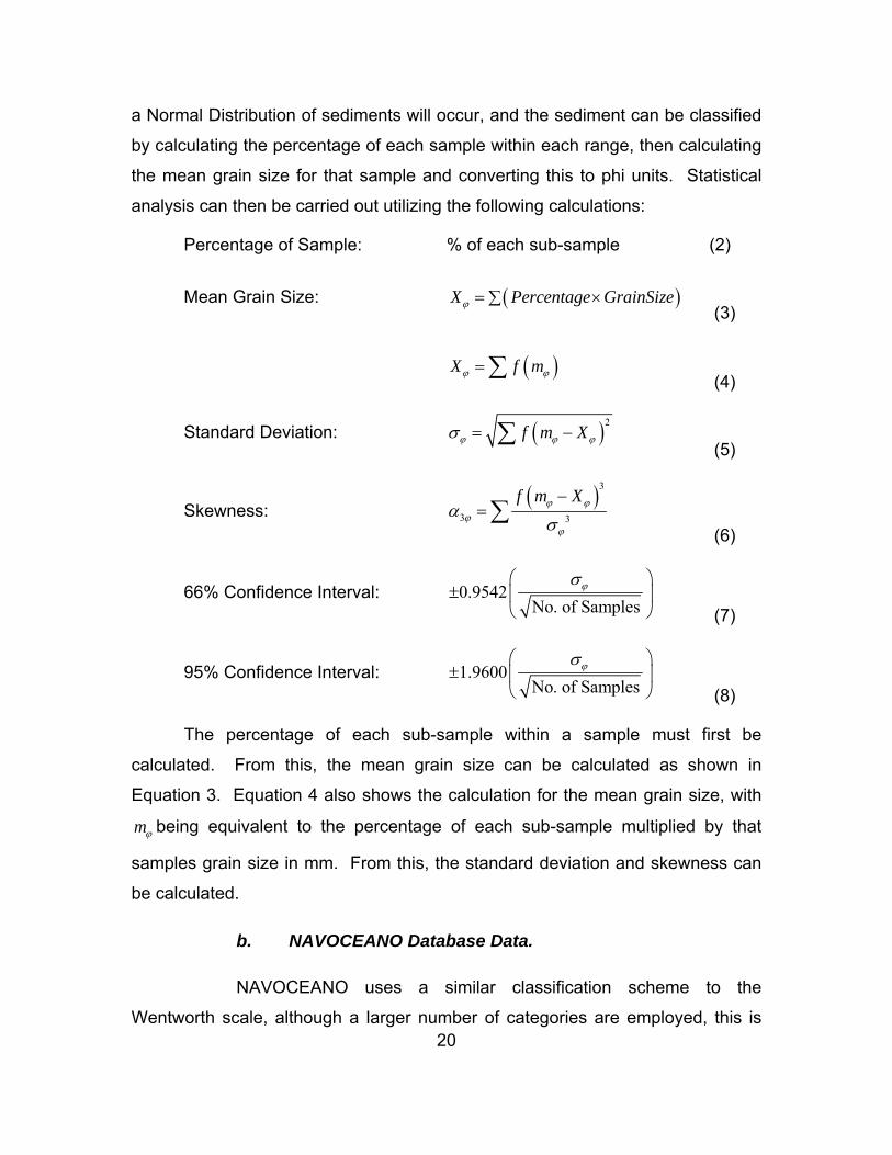
20

a Normal Distribution of sediments will occur, and the sediment can be classified

by calculating the percentage of each sample within each range, then calculating

the mean grain size for that sample and converting this to phi units. Statistical

analysis can then be carried out utilizing the following calculations:

Percentage of Sample: % of each sub-sample (2)

Mean Grain Size: ( )X Percentage GrainSizeϕ = ×∑ (3)

( )X f mϕ ϕ= ∑ (4)

Standard Deviation: ( )2f m Xϕ ϕ ϕσ = −∑

(5)

Skewness: ( )3

3 3

f m Xϕ ϕϕ

ϕ

ασ

−= ∑

(6)

66% Confidence Interval: 0.9542No. of Samples

ϕσ⎛ ⎞± ⎜ ⎟

⎝ ⎠ (7)

95% Confidence Interval: 1.9600No. of Samples

ϕσ⎛ ⎞± ⎜ ⎟

⎝ ⎠ (8)

The percentage of each sub-sample within a sample must first be

calculated. From this, the mean grain size can be calculated as shown in

Equation 3. Equation 4 also shows the calculation for the mean grain size, with

mϕ being equivalent to the percentage of each sub-sample multiplied by that

samples grain size in mm. From this, the standard deviation and skewness can

be calculated.

b. NAVOCEANO Database Data.

NAVOCEANO uses a similar classification scheme to the

Wentworth scale, although a larger number of categories are employed, this is

21

shown in Table 5. Surface sediment type data provided by NAVOCEANO can be

obtained at high and low spatial resolutions.

The databases include analysis of grabs and cores collected during

surveys from multiple sources. Low resolution data is based on data for every

five minutes of latitude and longitude. High resolution data is based on every six

seconds of latitude and longitude. In certain areas, including San Francisco Bay,

more detailed surveys have been compiled and the resolution is increased. In

this investigation sediment samples are compared to the High Frequency

Environmental Acoustics (HFEVA) dataset (NAVOCEANO, 2003).

Table 5. NAVOCEANO HFEVA database sediment classification. (From NAVOCEANO, 2003)

2. Grain Size Distribution and Fluid Flow

Grain size distribution and fluid flow are important in calculating sediment

transport. Sediment within a flow can be transported in three ways, along the

bed as bedload, in suspension as suspended load or along the air-water

22

interface as wash-load, the location at which the sediment will be located can be

determined by the Rouse Number:

s

os

wRuκ

= (9)

where ws is the setting velocity; κ = 0.407, is the von Karman constant; and su is

the shear velocity. The settling velocity of the sediment, ws, is determined by the

sediment density, ρs, and diameter, d of the sediment particle.

The required Rouse numbers for transport as bed load, suspended load,

and wash load are summarized in Table 6.

Table 6. Mode of transport related to Rouse numbers (From Wikipedia, 2009)

The shape of the grains also influences the settling velocity and therefore

the distribution of grains, as shown in Figure 5. As the size of the grains

increase, the settling velocity also increases, indicating that larger grains can

settle in regions with increased fluid flow, where as finer grains will settle in

regions with a lower fluid flow.

Mode of Transport Rouse Number

Bed load >2.5

Suspended load: 50% Suspended >1.2, <2.5

Suspended load: 100% Suspended >0.8, <1.2

Wash load <0.8

23

Figure 5. Settling velocities of grains in water at 20oC as a function of grain diameter and shape factor (From Komar and Reimers, 1978).

In this study, bedload transport is determined to be the most important

factor. The magnitude of bedload transport is extremely difficult to quantify, there

are a number of theories and studies that have been carried out, however, there

is no generic solution to this problem. Therefore, in order to determine survey

periodicity for mine warfare route surveys a qualitative approach is necessary at

this stage.

3. Threshold of Sediment Movement

The seabed is composed of individual sediment grains. The forces acting

upon each grain are summarized in Figure 6.

24

Figure 6. Forces acting on a grain resting on the seabed (From Liu, 2001)

The flow drag force on the grain is the driving factor, this is defined as:

FD =12

ρCDπd2

4αu*( )2

(10)

where the friction velocity u* is the flow velocity close to the seabed, α is a

coefficient used to modify the friction velocity, in turn *uα is the characteristic flow

velocity past the grain. The grain will start to move at critical friction velocity , this

can be denoted as *cu . This is the point at which the grain is about to move, and

occurs when the drag force is equal to the friction force that is parameterized as

the net vertical force (gravity – lift) multiplied by an empirical friction factor, f.

12

ρCDπd2

4αu*,c( )2

= f ρs − ρ( )g πd3

6−

12

ρCLπd2

4αu*,c( )2⎛

⎝ ⎜

⎞

⎠ ⎟ (11)

This equation is then rearranged:

u*,C2

s −1( )gd=

fα 2CD + fα 2CL

43α 2

(12)

The left hand side of the rearranged equation gives us the critical Shields

parameter, cθ , in turn the Shields parameter,θ can be defined as:

θ =u*

2

s −1( )gd (13)

25

Movement will occur if the Shields parameter is greater than the critical

Shields parameter. Figure 7 shows the thresholds of Shields parameter as

delineating suspended and bedload sediment as a function of grain size

according to Bagnold (1956) with a coefficient of 0.4 and McCave (1971) with a

coefficient of 0.19. The actual figures are still disputed.

Figure 7. Shields diagram showing the threshold of suspension (From Dyre, 1986)

B. BEDFORM FORMATION

When sediment begins to move bedforms will begin to form. A flat bottom

can become deformed, with a series of undulations. As water flow increases,

drag will be increased, and this increases in the shear stress available at the bed

to create grain movement (Dyre, 1986). In laboratory investigations, the

sequence of bedforms with increasing flow intensity is: Flat bed, Ripples, Dunes,

High Stage Plane Bed, followed by Antidunes. Terminology varies in different

studies. A diagrammatic representation of the flow over bedforms and their

movement is shown in Figure 8.

26

Figure 8. Flow over Ripples, Dunes and Antidunes (From Liu, 2001)

If the average current velocity, water depth and sediment size are known

factors, then the expected bedforms can be predicted by empirical diagrams, as

shown in Figure 9. The sediment size is represented by the settling velocity. In

this example, the ripple speed is also given so that the figure can be used to

estimate the bed-load transport, (Liu, 2001).

Figure 9. Bedform prediction diagram (From Liu, 2001)

27

1. Ripples

Ripples are formed at relatively weak flow intensity; the mean grain

diameter for ripple formation is less than 0.7 mm (Liu, 2001). From observations,

it is estimated that the average height and length of ripples are controlled by

grain size, they are typically; Hr =100d50 and Lr =1000d50.

2. Dunes

Dunes, also known as Sand Waves, have a very similar shape to ripples,

but are larger in size. The size of dunes is typically controlled by flow depth.

Dunes are formed by coarser sediments, with mean grain size greater than 0.6

mm (Liu, 2001). As flow intensity increases, the dunes will increase in size,

reducing the water depth at the crest of the dunes. The high velocity over the

crest can cause the dunes to become washed out forming a flat plane bed.

3. Antidunes

Antidunes are formed when the Froude number exceeds unity. The wave

height on the water surface is of the same order as the antidune height, this

causes instability in the surface wave, which can grow and break in an upstream

direction, causing the antidune to move upstream (Liu, 2001).

C. INFLUENCE OF CURRENTS AND WAVES ON BEDFORMS

Both currents and waves will influence the formation of bedforms, and

they will affect the type of bedform, its size, and its shape. The magnitude of

sediment transport due to currents and waves has been extensively studied,

however, no single solution exists due to the complexity of the problem and the

number of variables associated with it. Bedload transport formula have been put

forward by Meyer-Peter (1948), Kalinske-Frijlink (1952), Einstein-Brown (1950),

Bagnold (1946), and Bijker (1971). These methods are all complex and do not

28

provide a general solution, however all provide solutions within the same order of

magnitude. This study will therefore be qualitative rather than quantitative.

1. Currents

The typical pattern of bedform formation in a steady current is illustrated in

Figure 10, showing typical bedforms related to increased flow. The starting point

is a typical ripple pattern (A), in a steady current this will develop into dunes with

ripples superposed (B) as the current continues to flow dunes will form (C), they

will then become washed out dunes or in a transition phase (D). Following this,

still under the influence of a steady current, a plane bed will form (E). If the flow

continues to strengthen, antidunes may be formed.

Figure 10. Typical bedforms in order of increased stream power (From Deigaard, 1992)

In a steady current, at the point where sediment transport will begin to

occur the bed becomes unstable. Fine sediments will form ripples usually with a

length of less than 0.6 m and a height of less than 60 mm, ripple size is generally

independent of water depth in this case, (Deigaard, 1992). As current velocity

increases, total bed shear stress increases and the type of bedform will follow the

29

pattern shown in Figure 11. Bed shear stress, bτ , is shown as the vertical axis,

this is plotted against velocity, V, on the horizontal axis. As bτ and V increase

the progression of ripples, dunes, plane bed followed by anti-dunes at the higher

bτ and V values can be seen.

Figure 11. Relationship between total bed shear stress and flow velocity for different bedforms (From Deigaard, 1992)

If the current is oscillatory in nature the shape of the bedforms will be

amended; this is shown in Figure 12. The bedform shape in oscillatory flow is

shown in the upper part of the diagram, this can be compared with the bedform

shape in steady flow in the lower part. It can clearly be seen that in oscillatory

flow the bedform will have more defined peaks, whereas in steady flow, the

peaks will appear much smoother.

Figure 12. A) Bedform shape in oscillatory flow, B) Bedform shape in steady flow (From Deigaard, 1992)

30

2. Waves

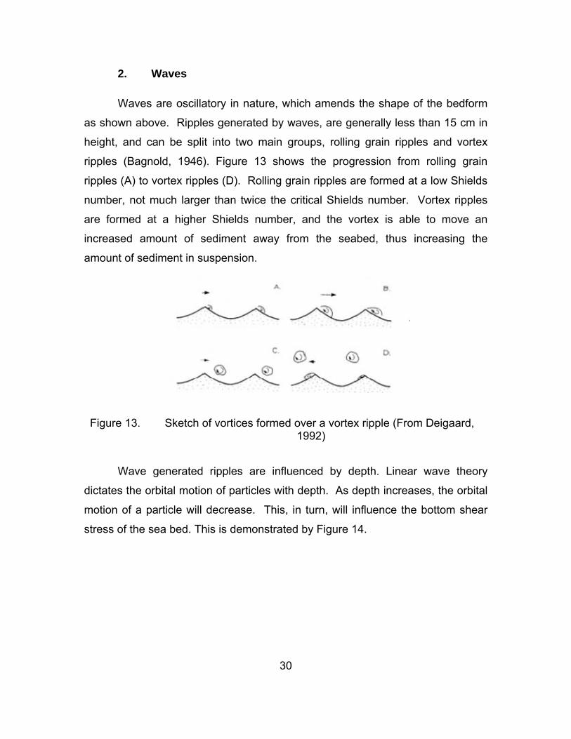
Waves are oscillatory in nature, which amends the shape of the bedform

as shown above. Ripples generated by waves, are generally less than 15 cm in

height, and can be split into two main groups, rolling grain ripples and vortex

ripples (Bagnold, 1946). Figure 13 shows the progression from rolling grain

ripples (A) to vortex ripples (D). Rolling grain ripples are formed at a low Shields

number, not much larger than twice the critical Shields number. Vortex ripples

are formed at a higher Shields number, and the vortex is able to move an

increased amount of sediment away from the seabed, thus increasing the

amount of sediment in suspension.

Figure 13. Sketch of vortices formed over a vortex ripple (From Deigaard, 1992)

Wave generated ripples are influenced by depth. Linear wave theory

dictates the orbital motion of particles with depth. As depth increases, the orbital

motion of a particle will decrease. This, in turn, will influence the bottom shear

stress of the sea bed. This is demonstrated by Figure 14.

31

Figure 14. Horizontal velocity profile and water particle orbit as predicted by linear wave theory (From Liu, 2001)

3. Combined Current and Wave Interaction

The general principle of sediment transport in the coastal or littoral region

is that waves stir up the sediment and currents, then in turn, transport the

sediment. When both waves and currents are present, wave induced velocity will

dominate the situation near to the bottom, even if the current velocity is much

larger. Because of the oscillatory motion of the waves, current will generally be

the main transport mechanism of sediment, except in breaking wave situations.

The comparison of current and wave velocity profiles is shown in Figure 15. The

velocity profile indicated by the solid line is that of wave induced velocity, the

dashed line indicates tidal current velocity. On the left, the differences

throughout the water column can be seen, with the tidal current velocity tending

to be the larger. On the right, the diagram shows a blow up of the region at the

seabed, where it can be seen that wave induced velocity is dominant.

32

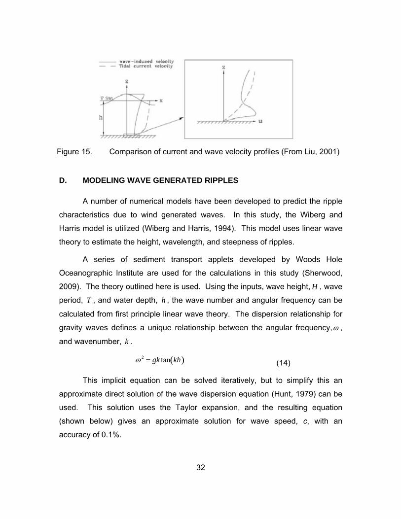
Figure 15. Comparison of current and wave velocity profiles (From Liu, 2001)

D. MODELING WAVE GENERATED RIPPLES

A number of numerical models have been developed to predict the ripple

characteristics due to wind generated waves. In this study, the Wiberg and

Harris model is utilized (Wiberg and Harris, 1994). This model uses linear wave

theory to estimate the height, wavelength, and steepness of ripples.

A series of sediment transport applets developed by Woods Hole

Oceanographic Institute are used for the calculations in this study (Sherwood,

2009). The theory outlined here is used. Using the inputs, wave height, H , wave

period, T , and water depth, h , the wave number and angular frequency can be

calculated from first principle linear wave theory. The dispersion relationship for

gravity waves defines a unique relationship between the angular frequency,ω ,

and wavenumber, k .

ω 2 = gk tan kh( ) (14)

This implicit equation can be solved iteratively, but to simplify this an

approximate direct solution of the wave dispersion equation (Hunt, 1979) can be

used. This solution uses the Taylor expansion, and the resulting equation

(shown below) gives an approximate solution for wave speed, c, with an

accuracy of 0.1%.

33

( )2 112 4 51 0.6522 0.4622 0.0864 0.0675c y y y y y

gh

−−⎡ ⎤= + + + + +⎢ ⎥⎣ ⎦ (15)

y =ω 2h

g (16)

c =ωk (17)

From this relation, the near bed orbital diameter 0d , and the near bottom

orbital velocity, orbU can be calculated:

d0 =H

sinh 2πh L( ) (18)

Uorb =πd0

T (19)

Using these results and the sediment grain size (mm), the ripple height,

ripple wavelength, ripple steepness, and classification can be determined as

detailed in Wiberg and Harris (1994).

Ripples are divided into three categories; this was determined by analysis

of ripple wavelengths. The ratio of near bed orbital diameter 0d and mean grain

diameter D, are examined. At small ratio values, ripple wavelength or spacing is

proportional to 0d ; these are referred to as orbital ripples (Clifton, 1976). At large

ratio values, ripple wavelength appears to be independent of 0d , but is roughly a

constant multiple of the grain size (~500D), which is referred to as anorbital

ripples (Clifton, 1976). In the intermediate range the ripples are termed

suborbital.

Wiberg and Harris examined experimental results from many previous

studies, and relationships determined. It was found that for orbital ripples a

simple linear relationship existed for ripple wavelength and steepness.

λorb = 0.62d0 (20)

34

ηλ

⎛ ⎝ ⎜ ⎞

⎠ ⎟

orb= 0.17

(21)

For anorbital ripples the relationship was more complex:

λano = 535D (22)

ηλ

⎛ ⎝ ⎜ ⎞

⎠ ⎟

ano= exp −0.095 ln d0

η⎛

⎝ ⎜

⎞

⎠ ⎟

2

+ 0.442ln d0

η− 2.28

⎡

⎣ ⎢ ⎢

⎤

⎦ ⎥ ⎥ (23)

For suborbital ripples a weighted geometric average bounded by the

wavelengths of anorbital and orbital ripples was determined giving:

λsub = expln d0 ηano( )− ln100

ln20 − ln100⎛

⎝ ⎜

⎞

⎠ ⎟ lnλorb − lnλano( )+ lnλano

⎡

⎣ ⎢

⎤

⎦ ⎥ (24)

Wiberg and Harris, guided by previous studies, argued that the most

important difference between orbital and anorbital ripples is the ratio of wave

boundary layer thickness to ripple height, which can be approximated by the ratio

0dη . Using this criteria:

0dη < 20 orbital ripples (25)

0dη > 100 anorbital ripples (26)

20 < 0dη < 100 suborbital ripples (27)

Using this theory from three simple inputs, the ripple characteristics can

be approximated, however, the ripple geometries are limited, with one of the

main factors being depth. The calculations are limited to sand sized sediments, it

also suggests that there may be no transport if the near bottom orbital velocity is

less than 0.13 cm/s. Figures 16 and 17 show the results obtained by this model.

35

Figure 16 shows the near bottom orbital velocity for different wave heights

and different wave periods plotted against depth. It can be seen that as wave

height increases, so does the near bottom orbital velocity. The same is true for

an increased wave period, which also increases the near bottom orbital velocity.

It can also be seen that, in each case, the near bottom orbital velocity increases

initially with an increase in depth. A maximum is reached at depths between 10

m and 15 m, the near bottom orbital velocity then steadily decreases with depth,

in all cases at depths greater than 60 m the near bottom orbital velocity had

reduced to 0.2 m/s or less.

Figure 17 shows the wave generated ripple heights for a 1 m wave. The

ripple height is plotted against depth for different wave periods and three different

sediment sizes, with phi 2.5, corresponding to fine sand, phi 1.5, corresponding

to medium sand, and phi 0.5, corresponding to coarse sand. It can be seen that

the ripple heights are larger for the coarse sand and reduce as the sand

becomes finer. As wave period increases the ripple heights also increase. Peak

ripple heights are found at approximately 10 m to 15 m depth, which corresponds

to the maximum near bottom orbital velocities.

36

Figure 16. Differences in near bottom orbital velocity for different wave heights and wave periods, for a sediment size of 2.5phi, results obtained using

the Wiberg and Harris model

37

Figure 17. Differences in wave generated ripple heights for different wave

periods and sediment size, for a wave with a height of 1 m, results obtained using the Wiberg and Harris model

38


39

III. CASE STUDY: SAN FRANCISCO BAY

A. INTRODUCTION

San Francisco Bay is a large, shallow, dynamic estuary located in

California on the west coast of the U.S. It is a major international shipping port,

with large container facilities, which makes it a significant, economically important

port. It is an extremely busy waterway used by both commercial and recreational

vessels. San Francisco Bay is thought to have been formed by a down-warping

of the Earth’s crust between the San Andreas Fault to the west and the Hayward

Fault to the east.

The area has been subject to major changes in topography through the

years. In the nineteenth century, the area was subjected to hydraulic mining,

which released massive amounts of sediment that settled in areas of the bay with

little or no currents. In the twentieth century, the Army Corp of Engineers began

to carry out dredging operations, which have continued. Also aggregate mining

has occurred in this region. These activities have all had an impact on the area,

although the impact has not been quantified (Army Corp of Engineers, 1996;

Friends of the Estuary, 1997).

Approximately 40% of water drainage from the central coast rivers enters

the Pacific Ocean through the Golden Gate channel. This represents a mean

high freshwater discharge rate of approximately 800 m3/s (California Department

of Water Resources, 2007). This is a huge amount of fresh water entering the

estuarine system, which has the potential to carry a significant amount of

sediment into the area.

The San Francisco Bay area is subject to a complex semi-diurnal tidal

regime, this leads to temporally and spatially variable currents that can exceed

2.5 m/s. This leads to a diverse and complex pattern of bedform formations,

40

which were first mapped using side-scan sonar in the late 1970’s, and are now

mapped using high resolution multi-beam surveys. (Barnard et al., 2007).

In this chapter, the Golden Gate region is investigated in detail. A

comparison study of localized sediment grab data in the same positions for a

three year period is assessed and analyzed. This data is then compared to the

NAVOCEANO HFEVA sediment database, and an assessment of the validity of

this database is made. Multi-beam data, obtained by the USGS is examined and

the impact of these findings on the mine warfare route survey periodicity

assessed.

B. SEDIMENT ANALYSIS: COMPARISON OF LOCALIZED SAMPLE DATA AND DATABASE DATA

In February 2009, sediment samples were collected in the vicinity of the

Golden Gate region of San Francisco Bay. Previous sediment studies had been

carried out in the winters of 2007 and 2008. The intent of this investigation is to:

1) re-visit the previously sampled sites and determine statistically if there has

been a change in the sediment properties, and 2) compare the latest sediment

samples to the NAVOCEANO HFEVA database to determine if the database

remains valid.

1. Data and Methods

Sediment samples were collected during a student cruise in the winter of

2009 (OC3570 Operational Oceanography course). The cruise took place from

29 January until 4 February 2009, onboard the R/V Point Sur. Four sediment

samples were collected in San Francisco Bay. The sample locations were the

same as those that had been previously sampled during the Winter 2007/2008

cruises.

41

a. Sediment Sample Collection

The samples were all collected using a double trap Van Veen

sediment grab, deployed off the stern of the ship using a crane. The Van Veen

grab is a light weight stainless steel sampler designed to take samples of soft

bottom sediment. Water is able to flow through the grab as it is lowered. When it

hits the seabed, the doors of the grab close due to tension on the cable, they

remain closed while the grab is raised and recovered on deck.

Figure 18. Van Veen grab on board R/V Point Sur.

Upon recovery of the grab a representative sample of the sediment

was then collected in a quart mason jar. The jar was then sealed, labeled and

stored, for laboratory processing.

b. Sediment Sample Analysis.

The sediment sample analysis was conducted in the oceanographic

laboratory at the Naval Postgraduate School. Laboratory analysis can be broken

down into phases.

The first phase involved emptying the contents of each jar into a

standard plastic Rubbermaid basin; the sample was rinsed with fresh water while

being agitated. The sample was then left to settle—the time this took depended

42

on the consistency of the sample, with silty samples taking much longer. The

samples were generally left overnight; this allowed all the sediment to return to

the bottom, leaving clear water on top. Following the settling period, any

particulates or biologic material floating on the water was removed. The fresh

water was then decanted out, being careful not to pour out any sediment. If

necessary, this process was repeated.

The rinsed sediment was then transferred into a pre-weighed 8 x 8

inch, Pyrex casserole dish. Sediment was transferred by pouring, scraping using

a spoon, and rinsing by squeezing a fine stream of water into the bowl. Once

transferred, the sample was placed in the laboratory oven overnight to dry. The

oven was set at approximately 90o C. Once the sample was completely dry, it

was weighed and prepared for the sieving process.

The dried sample was broken up, in some cases this could be

achieved by using a spoon. However it was necessary to use a hammer to break

up some of the more difficult samples. These tended to be the finer samples that

had become like baked clay. The broken up sample was then place in a pre-

weighed plastic bag. The bagged sample was weighed and the result recorded.

The next phase, the sieving phase was achieved by using a Ro-

Tap automated sieve. A 100 ml glass beaker was weighed, a quantity of the

sample was added to the beaker and it was re-weighed, both weights were

recorded. This was the part of the sample to be analyzed. The Ro-Tap sieve

used in this experiment utilized 14 sieves ranging from 2.00 mm to 0.070 mm in

mesh diameter.

The sample was poured into the top sieve (2.00 mm), and then

sieved through the column of sieves for 15 minutes. The sample collected in

each sieve was carefully collected, by pouring it onto a sheet of card and

removing any residue from the sieve with a wire brush, it was then transferred

43

into a pre-weighed plastic bag. The bag and sample was then weighed and the

results recorded. A loss of less than 1% of the sediment weight had to be

achieved if the result was to be deemed accurate.

c. Localized Sample Data.

The samples collected were compared to samples collected on the

2007/2008 cruises. The previous results were re-formatted for comparison.

Figure 19. Locations of the localized samples used for comparison.

Statistical analysis was carried out; the results for each sample

were first normalized to allow comparison to take place. Analysis as described in

Chapter II was used (Dyre, 1986) to estimate the mean grain size, and classify

the sediment sample according to the Wentworth scale.

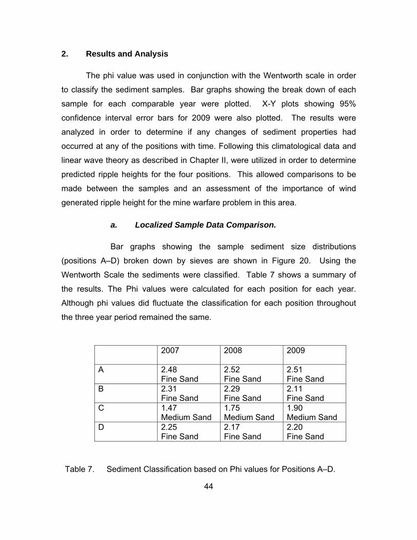
44

2. Results and Analysis

The phi value was used in conjunction with the Wentworth scale in order

to classify the sediment samples. Bar graphs showing the break down of each

sample for each comparable year were plotted. X-Y plots showing 95%

confidence interval error bars for 2009 were also plotted. The results were

analyzed in order to determine if any changes of sediment properties had

occurred at any of the positions with time. Following this climatological data and

linear wave theory as described in Chapter II, were utilized in order to determine

predicted ripple heights for the four positions. This allowed comparisons to be

made between the samples and an assessment of the importance of wind

generated ripple height for the mine warfare problem in this area.

a. Localized Sample Data Comparison.

Bar graphs showing the sample sediment size distributions

(positions A–D) broken down by sieves are shown in Figure 20. Using the

Wentworth Scale the sediments were classified. Table 7 shows a summary of

the results. The Phi values were calculated for each position for each year.

Although phi values did fluctuate the classification for each position throughout

the three year period remained the same.

2007 2008 2009

A 2.48 Fine Sand

2.52 Fine Sand

2.51 Fine Sand

B 2.31 Fine Sand

2.29 Fine Sand

2.11 Fine Sand

C 1.47 Medium Sand

1.75 Medium Sand

1.90 Medium Sand

D 2.25 Fine Sand

2.17 Fine Sand

2.20 Fine Sand

Table 7. Sediment Classification based on Phi values for Positions A–D.

45

Figure 20 shows the breakdown of percentage sample mass for

each position and each year. The largest grain size is shown on the left and the

smallest on the right. Each column represents the percentage of sample mass

recovered from each of the 14 sieves and the bottom pan. The actual sediment

sizes are shown in Figure 21 where a more detailed statistical analysis was

carried out. Each bar graph shows that the sieve with the highest percentage of

sample mass for each position remained the same in each year. These results

would indicate that the sediment characteristics for all positions have changed

little, and sediment classification remains unchanged for the 2007 to 2009 period.

46

47

Figure 20. Column Graphs for positions A–D, showing sample breakdown, per year, from largest grain size (left) to smallest grain size (right)

48

49

Figure 21. Sample mass (%) v’s grain size (mm) for positions A to D. Error

Bars indicate the 95% Confidence Interval in both dimensions.

50

Figure 21 shows the same breakdown of sediment samples by

grain size, with 95% confidence intervals. Although there are differences

between the distributions for each year these variations are not significant at a

95% confidence level. Thus, the main conclusion is that the sediment

characteristics have not changed considerably within the three year period.

b. Comparison of Ripple Heights

Table 8 shows the estimated ripple heights from waves and

characteristics for positions A to D. The wave conditions were obtained from

marine gridded climatology data provided by Fleet Numerical METOC

Detachment in Ashville. Values were calculated by re-analysis of data from 1857

to 1997.

Position A results show all the ripples classed as orbital, the ripple

height varies from 0.3 cm to 0.4 cm. This indicates a limited amount of variability

at position A over the time period.

Position B results also show the ripples are classified as orbital in

all cases. The ripple heights vary from 2.5 cm to 3.1 cm. Although this position

has more variability it remains at less than 1 cm, so cannot be deemed

significant.

Position C results, again, classify the ripples as orbital, while the

ripple height varies from 1.9 cm to 3.1 cm. Although the variability is slightly

larger than the other two positions the range of ripple heights remains relatively

small and inconsequential.

Position D shows the largest variability, all ripples remain orbital,

but heights range from 1.4 cm to 3.4 cm. The range of phi values is from 2.17 to

2.25, which is not a large range, however the depth at which the grab samples

were obtained is more variable for this position, which could explain the variability

in results. The difference of 2 cm ripple height over a three year period is not

large enough to be a significant problem.

51

From these results, it can be seen that the ripple heights for each

position show a degree of variability, although not on a large scale. The variation

for each position is in the order of centimeters, the estimated ripple heights from

waves are all relatively small and would be inconsequential for mine burial at

these positions. However, this does not take into account the currents in this

region.

Although the ripple height is assessed as too small to bury a mine it

still remains an important issue in the mine warfare survey periodicity problem.

Smaller ripples in the order of centimeters can cause a significant problem in

mine detection due to scattering of acoustic rays.

52

2007 2008 2009 Mean SD

A Phi 2.48 2.52 2.51 2.50 0.02

Depth (m) 60 63 63 62 1.73

Orbital Diameter (mm) 0.019 0.015 0.015 0.016 0.0023

Orbital Velocity (m/s) 0.017 0.013 0.013 0.014 0.0023

Ripple Height (cm) 0.4 0.3 0.3 0.33 0.0577

Ripple Classification Orbital Orbital Orbital

B Phi 2.31 2.29 2.11 2.23 0.11

Depth (m) 37 35 38 36.6 1.52



Ripple Height (cm) 2.7 3.1 2.5 2.77 0.3055


C Phi 1.47 1.75 1.90 1.71 0.21

Depth (m) 38 41 35 38 3.00



Ripple Height (cm) 2.5 1.9 3.1 2.5 0.6


D Phi 2.25 2.17 2.20 2.21 0.04

Depth (m) 40 45 34 39.67 5.508



Ripple Height (cm) 2.1 1.4 3.4 2.3 1.01


Table 8. Ripple Characteristics for positions A–D.

53

c. NAVOCEANO Database Comparison.

The four samples were compared to the NAVOCEANO HFEVA

database. Results are summarized in Table 9.

Phi Wentworth Sediment Classification

HFEVA Database

A 2.51 Fine Sand Fine Sand B 2.11 Fine Sand Fine Sand C 1.90 Medium Sand Medium Sand D 2.20 Fine Sand Fine Sand

Table 9. 2009 sediments samples compared to NAVOCEANO Database Data.

Figure 22. Positions A–D, overlaid on the NAVOCEANO HFEVA Dataset.

54

Table 9 shows that the classifications of each of the four positions

are the same as the NAVOCEANO database data. Figure 22 shows the

NAVOCEANO HFEVA dataset plotted geographically; each color represents a

different sediment type as shown in the key on the left of the figure. Figure 22

also shows that the experimental results compare well with the database data.

The experimental results all fall within the same sediment categories that the

database predicts. This would suggest that this is a valid database. Positions A,

B and D all fall within the fine sand category geographically, and position C falls

within the (medium) sand category.

d. Accuracy and Errors.

There are issues involving the accuracy and errors associated with

this investigation. Although, during the collection and laboratory processing, as

much care as possible was taken to limit or eliminate errors.

During the collection phase, the bridge of the R/V Point Sur was

given the positions of previously collected samples, the ship aimed to stay in

station at these locations as accurately as possible during the deployment and

retrieval of the grab. However, from comparing the positions over the three

years, it can be noted that although the positions are extremely similar, they are

not exactly the same. This is reflected in the depths used in calculating ripple

height and is the main reason for the variation in the ripple height.

In order to gain a better representation of sediment type, it would

be preferable to take a selection of samples at each position, so that the average

result could be used, rather that relying on one sample. This would allow any

erroneous sediment samples to be excluded, or have a minimal effect on the

results used for comparison. There results, used for comparison from previous

studies, were assumed to be correct, the sediment samples were not available

for re-analysis.

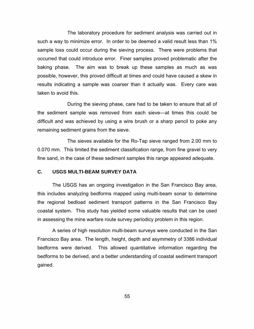
55

The laboratory procedure for sediment analysis was carried out in

such a way to minimize error. In order to be deemed a valid result less than 1%

sample loss could occur during the sieving process. There were problems that

occurred that could introduce error. Finer samples proved problematic after the

baking phase. The aim was to break up these samples as much as was

possible, however, this proved difficult at times and could have caused a skew in

results indicating a sample was coarser than it actually was. Every care was

taken to avoid this.

During the sieving phase, care had to be taken to ensure that all of

the sediment sample was removed from each sieve—at times this could be

difficult and was achieved by using a wire brush or a sharp pencil to poke any

remaining sediment grains from the sieve.

The sieves available for the Ro-Tap sieve ranged from 2.00 mm to

0.070 mm. This limited the sediment classification range, from fine gravel to very

fine sand, in the case of these sediment samples this range appeared adequate.

C. USGS MULTI-BEAM SURVEY DATA

The USGS has an ongoing investigation in the San Francisco Bay area,

this includes analyzing bedforms mapped using multi-beam sonar to determine

the regional bedload sediment transport patterns in the San Francisco Bay

coastal system. This study has yielded some valuable results that can be used

in assessing the mine warfare route survey periodicy problem in this region.

A series of high resolution multi-beam surveys were conducted in the San

Francisco Bay area. The length, height, depth and asymmetry of 3386 individual

bedforms were derived. This allowed quantitative information regarding the

bedforms to be derived, and a better understanding of coastal sediment transport

gained.

56

Selections of USGS survey results are shown in this section (With

permission, Barnard, 2007/2009), the effect of these findings on the survey

periodicity problem are discussed. The results are also used as a quality control

measure in determining a survey periodicity model for this area and are

discussed in Chapter IV.

1. Bed Patterns in San Francisco Bay

Figures 23 and 24 show detailed multi-beam images of the San Francisco

Bay region. The complexity and variety of the bedforms in this region can clearly

be seen in these images.

57

Figure 23. Bedforms in the inlet throat of San Francisco Bay (With Permission,

from Barnard et al., 2007)

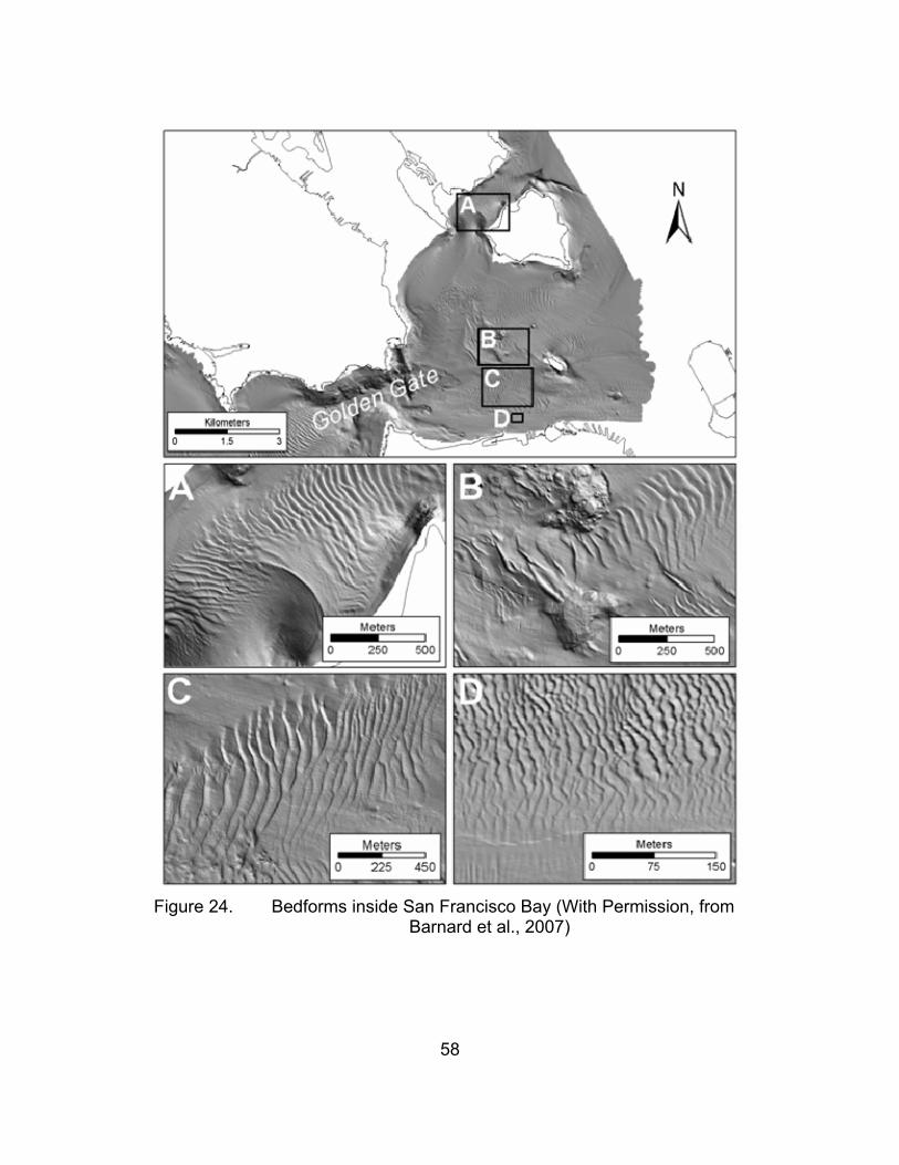
58

Figure 24. Bedforms inside San Francisco Bay (With Permission, from Barnard et al., 2007)

59

2. Temporal Variation in Bedform Morphology

In the region of the larger bedforms, a number of surveys were conducted.

The time scale of these surveys ranged from a few hours to more than ten years.

Transects through these areas were analyzed to determine if bedform size and

shape varied significantly, and on what time scales these variations occur. The

USGS concluded that the bedform fields, as a whole, maintained relative

symmetry, and that asymmetry values have not changed markedly with time

(Barnard et al., 2007).

Figure 25 shows two transects. The first, in the mouth of San Francisco

Bay (Transect B), was repeatedly surveyed in a 5.5 hour period in September

2005. It shows sand wave heights of approximately 5 m. These are large

bedforms compared with for example the size of a MANTA mine (height

approximately 0.5 m), and understanding their evolution is of great importance to

the mine warfare community The second transect, (Transect C) the Alcatraz

Shoal region, was surveyed from time scales of two weeks to eleven years, again

it can be seen that although the height of the sand wave peaks do not vary

considerably, their location does.

Figures 26 and 27 show the results from April and November 2008, in the

region between Alcatraz and Angel Island, again it can be seen in the depth

profile A-B, that the heights of the sand wave peaks do not vary considerably but

their location does. This area is further complicated, smaller bedforms are super

imposed on the larger ones, this can be seen more clearly in transect C-D. The

super imposed bedforms were only identified in the later survey with use of

higher resolution multi-beam technology, and represent an additional change in

height of 0.4 m.

From the transects, it can be seen that the height of the sand wave peaks

does not vary considerably with time, however, the location of the peak does

move with time. This is significant for the mine warfare route survey periodicity

60

problem. The movement of the sand waves would cause a mine to be buried,

and hence not be detected during a survey, these regions should therefore be

subject to a higher survey periodicity.

61

.

Figure 25. A) Location of sand wave transects. B) Transect from mouth of San Francisco Bay. C) Transect in vicinity of Alcatraz Shoals. (With

permission, from Barnard et al., 2007)

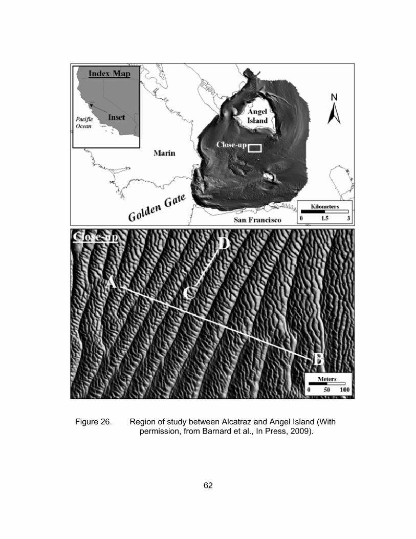
62

Figure 26. Region of study between Alcatraz and Angel Island (With permission, from Barnard et al., In Press, 2009).

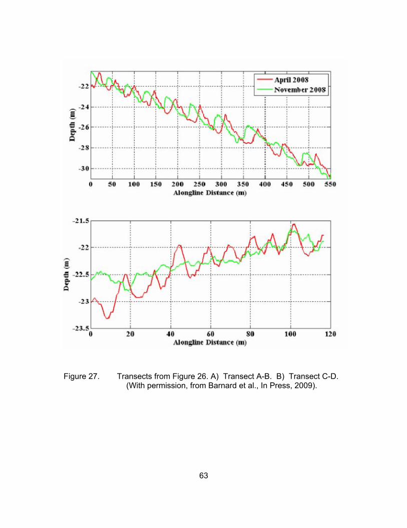
63

Figure 27. Transects from Figure 26. A) Transect A-B. B) Transect C-D.

(With permission, from Barnard et al., In Press, 2009).

64

3. Bedform Asymmetry and Sediment Transport Patterns

Detailed high resolution multi-beam data surveys have enabled an

assessment to be made of the relationship between bedform patterns and

dominant tidal transport directions. This can be seen in Figure 28, the

intersecting bedform patterns occur a) where a flood channel cuts obliquely

across alongshore migrating ebb-orientated bedforms and b) in a large region of

onshore directed bedform migration.

Figure 28. Complex current patterns offshore of Ocean Beach (with permission, from Barnard et al., 2007).

The asymmetry of bedforms in the region of the Golden Gate has been

assessed. This is shown in Figure 29, it shows that in the southern region the

bedforms are flood dominated, and in the northern region bedforms are ebb

dominated. From this the inferred net bedload sediment transport directions can

be determined; this is shown in Figure 30. The USGS used this information,

coupled with tidal information to develop a hydrodynamically calibrated numerical

model to predict total mean sediment transport, instantaneous water discharge

and sediment transport through the Golden Gate.

65

Figure 29. Asymmetry values across the Golden Gate (with permission from Barnard et al., 2007).

66

Figure 30. Inferred net bedload sediment transport directions based on

asymmetry values, arrows indicated direction only, not magnitude (with permission, from Barnard et al., 2007).

67

IV. DETERMINING ROUTE SURVEY PERIODICITY FOR SAN FRANCISCO BAY

A. INTRODUCTION

In order to determine the mine warfare route survey periodicity for San

Francisco Bay, a weighted suitability GIS model, utilizing a similar methodology

to the UKHO model, was developed. From the background theory in Chapter II

and the findings based on information in Chapter III, it is hypothesized that

waves, tides, currents and sediment size will influence bedform formation and

sediment processes; this in turn will affect the survey periodicity requirement.

Tidal data, from NAVOCEANO predictions is examined and the variability

in this region is shown. Historical current data, provided by NAVOCEANO is

analyzed. Using linear wave theory and climatological data, the estimated wave

generated ripple heights are calculated. Sediment data obtained from grab

samples provided by USGS is utilized. This data is weighted and combined, and

a model for survey periodicity is obtained.

This chapter details the process used to develop the survey periodicity

model for the San Francisco Bay region, it details the input layers used and the

weighting schemes employed. A number of different options based on various

weightings are reviewed and the most representative one chosen based on the

actual conditions found from the high resolution multi-beam data collected by

USGS.

B. THE MODELING CONCEPT

The concept of the weighted suitability model used here is summarized in

Figure 31. It utilizes three main input layers; predicted bedform type (green),

predicted bottom current (blue) and predicted wave generated ripple height (red).

Each of these layers can be thought of as a sub-model, similar to those used in

the UKHO model. The details of each layer is described in the following section.

68

Figure 31. Flow chart showing the three layers used to predict survey periodicity.

1. The Input Layers

a. Predicted Bedform Type

In order to predict the bedform type, 174 grab samples were

obtained from the USGS. The grab samples were taken during surveys dated

between 2004 and 2008. In addition the grab samples detailed in Chapter 3

were also included. The data included latitude, longitude, depth, and sediment

grain size. The dataset was compiled in excel and entered into the GIS software

program ArcMap. The data points were interpolated into a raster dataset and

classified using the Wentworth scale. The interpolated sediment classifications

are shown in Figure 32, with the positions of the grabs samples

69

overlaid. A graduated color scale is used with red representing the coarsest

sediments and blue representing the finest. It can be seen that the coarsest

sediment can be found in the mouth of the Golden Gate region.

Figure 32. Sediment type calculated from grab samples, locations of the grab samples are overlaid.

From background theory discussed in Chapter II, it is assessed that

ripples will be generated if the sediment grain size is less than 0.7 mm, these are

generally formed by wave motion. If the sediment size is greater than 0.6 mm

sand waves are more likely to form, these are generally due to current motions.

Taking this into account the grain size in mm was calculated and re-plotted, the

results are shown in Figure 33. Potential areas of wave generated ripples is

shown in green, this indicates a sediment size of less than 0.6 mm,

70

potential areas of current induced sand waves are shown in red, indicating a

sediment size greater than 0.7 mm. An intermediate zone between 0.6 mm and

0.7 mm is shown in yellow.

Figure 33. Potential bedform areas.

When Figure 33 is compared to the multi-beam data shown in

Figures 23 and 24, similarities can be easily identified. The regions identified as

current initiated sand waves tie in well with the sand wave fields observed in the

multi-beam surveys. This indicates that the theoretical assessment, that

sediment grain size is an important factor in the generation of bedforms, is

correct.

71

b. Predicted Bottom Currents

In order to obtain the predicted bottom currents, a number of data

sources were examined. The tidal regime in the San Francisco Bay area is

primarily semi-diurnal, however, it is extremely complex. Tidal prediction data

was obtained from NAVOCEANO. In order to predict the tidal heights in this

region, NAVOCEANO had split it into a number of different zones and the tide in

each zone is predicted separately due to the variability of tidal height in the

region. Tidal curves were plotted from the data provided, the tidal height is

relative to Mean Sea Level and the times were referenced to GMT. Figure 34

shows the zones in the region of study and Figure 35 shows a selection of the

plotted tidal curves. The tidal curves demonstrate the variability of tidal height in

this region. Six tidal curves are shown, the first is located at the mouth of the

Golden Gate, zone 37, and then proceed Northeast inshore to zone 12.

Figure 34. Tidal Zones in the San Francisco Bay region.

72

Tidal Curve: Zone 37

-5

-4

-3

-2

-1

0

1

2

3

4

5

6

1 Jan 09 - 5 Feb 09

Hei

ght (

m)


-5

-4

-3

-2

-1

0

1

2

3

4

5

6

1 Jan 09 - 5 Feb 09

Hei

ght (

m)


-5

-4

-3

-2

-1

0

1

2

3

4

5

6

1 Jan 09 - 5 Feb 09

Hei

ght (

m)


-5

-4

-3

-2

-1

0

1

2

3

4

5

6

1 Jan 09 - 5 Feb 09

Hei

ght (

m)


-5

-4

-3

-2

-1

0

1

2

3

4

5

6

1 Jan 09 - 5 Feb 09

Hei

ght (

m)


-5

-4

-3

-2

-1

0

1

2

3

4

5

6

1 Jan 09 - 5 Feb 09

Hei

ght (

m)

Figure 35. Tidal Curves in the San Francisco Bay Region

73

The complexity of the tidal regime leads to a complex system of

tidal currents. It was decided, that in this study, tidal height would not be a

suitable parameter to use. However, the tidal data is taken into account by the

historical current data for this region. In this model data from NOAA has been

utilized. Over 50 current stations were analyzed, the data included latitude,

longitude, depth and mean annual ebb and flood currents for each station. This

data includes the currents due to tides. The data was imported into MS Excel

and then directly imported into ArcMap. The data was separated into surface

currents and bottom currents. Locations of the current stations are shown in

Figure 36.

Figure 36. The locations of the current station data used.

74

Both the mean ebb and mean flood surface current data was

plotted with the arrows indicating the magnitude and direction of the current at

the station location. Red arrows indicate ebb currents and green arrows indicate

flood currents. The bottom currents were plotted in the same manner. The

results are shown in Figure 37 (surface currents) and Figure 38 (bottom

currents).

Figure 37. Surface currents, arrows indicate the magnitude and direction of the current, red indicates ebb currents, green indicates flood currents.

Figure 38. Bottom currents, arrows indicate the magnitude and direction of the current, red indicates ebb currents, green indicates flood currents.

Graduated depth scale shown in meters.

75

Due to the importance of flood and ebb dominated currents in

bedform formation, further interpolation of this data was conducted. The currents

were interpolated into a raster dataset and separated into ebb dominated and

flood dominated regions. Ebb currents were assigned a negative value, and

flood currents were assigned a positive value and the residual differences

between the two calculated. The results of this interpolation are shown in Figure

39. Ebb dominated regions are indicated in red and flood dominated regions are

shown in green. The contours indicate current speed, and are plotted at 0.1 m/s

intervals, with the interface between the ebb and flood regions being 0.

Figure 39. Ebb and flood dominated regions, surface currents (left), bottom currents (right).

From Figure 39, a good insight into the circulation patterns of San

Francisco Bay can be gained. The general circulation pattern is similar to that in

the Straits of Gibraltar, with an influx of saline water at the bottom and an out flow

of fresh water at the surface. Examination of the representation of bottom

currents shows some interesting features. When compared with the asymmetry

of bedforms generated by USGS (Figure 29), extremely good correlation is

noted. When compared with the multi-beam data, (Figures 23 and 24), it can be

seen that where the boundary between ebb and flood dominated regions occur,

76

bedforms also occur. This is particularly noticeable to the north of Angel Island,

in the region of the Alcatraz Shoal and in the inlet throat of the Bay. This layer

was therefore selected for use in the survey periodicity model.

c. Predicted Wave Generated Ripple Heights

To calculate the mean wave generated ripple heights, the theory

described in Chapter II was utilized. The grab samples provided latitude,

longitude, depth and sediment size data. This data was used in conjunction with

marine gridded climatology data obtained from Fleet Numerical METOC

Detachment in Ashville. The climatological data is calculated by re-analysis of

data from 1857 to 1997. Example data for the months of January and July are

shown in Table 10.

January July Sea Surface Temp (oC) 10-12 14 - 16 Salinity (psu) 32 32 Wind Speed (m/s) 7-8 4-5 Wind Direction (deg) 020 080 Wave Direction (deg) 270 270 Wave Height (m) 2.74 -3.66 0.91-1.83 Wave Period (s) 7 5 Significant Wave Height (m) 1.83 – 2.74 0.91 – 1.83 Swell Direction (deg) 270 270 Swell Height (m) 1.83 – 2.74 0.91 – 1.83 Swell Period (s) 6-9 6-9

Table 10. Climatological data used in this study.

Using linear wave theory, the depth, mean wave height and mean

wave period, the near bottom orbital velocity and near bottom orbital diameter

were calculated. Applying the Wiberg and Harris model, and including the

sediment grain size data the predicted ripple height was calculated. This data

was collated in MS Excel and then imported into ArcMap. The data was

77

interpolated into a raster data set. Layers were generated for the monthly mean

data, these were then combined in order to generate an annual mean wave

generated ripple height layer. Examples of the layers generated for January,

July and the mean wave generated ripple heights are shown in Figure 40. The

smaller ripple heights are shown in pink, with the greatest ripple heights shown in

orange and brown, as according to the color scale shown. It can be seen that

the greatest ripple heights occurred seaward of the San Francisco Bay region in

January, this coincided with the larger wave heights.

Figure 40. Mean wave generated ripple heights in cm, for January (left) and July (right).

In certain regions, under specific circumstances, for example where

the waves are too small in deep channels, there are no ripples generated from

the waves, as the near bed orbital velocity and near bed orbital diameter are not

large enough to generate ripples. In cases where this occurred the value was

classified as ‘Exceeds Limits’, this is shown in white, and can be seen in the

Golden Gate region in July. When this occurred a value of -0.1cm was assigned

to that data point, this was then classified as exceeding limits in the resulting

layers. Figure 41 shows a mean ripple heights layer that was selected for use in

the survey periodicity model. This layer is a composite of the monthly layers

generated, and each monthly layer was given an equal weighting. The larger

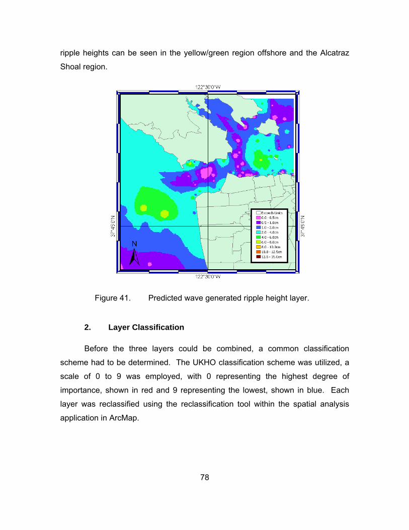
78

ripple heights can be seen in the yellow/green region offshore and the Alcatraz

Shoal region.

Figure 41. Predicted wave generated ripple height layer.

2. Layer Classification

Before the three layers could be combined, a common classification

scheme had to be determined. The UKHO classification scheme was utilized, a

scale of 0 to 9 was employed, with 0 representing the highest degree of

importance, shown in red and 9 representing the lowest, shown in blue. Each

layer was reclassified using the reclassification tool within the spatial analysis

application in ArcMap.

79

a. Predicted Bedform Type

It is assessed that large bedforms will occur when sediment sizes

are larger; these are likely to be current induced bedforms. Larger sediment

sizes were assigned a higher weighting and the weighting reduced with reducing

sediment size. The weighting scheme is detailed in Table 11 and the resulting

layer shown in Figure 42. Figure 42 shows the largest sediment sizes in red, in

accordance to the colored weighting scheme shown. The largest sediments

occur in the Golden Gate region and the Alkatraz Shoal region, this also

corresponds to deeper water and strong currents.

Sediment Size (mm) Weighting

>0.7 0

0.6 – 0.7 1

0.5 – 0.6 2

0.4 – 0.5 3

0.3 – 0.4 4

0.2 – 0.3 5

0.1 – 0.2 6

0.05 – 0.1 7

0.01 – 0.05 8

<0.01 9

Table 11. Weighting scheme for sediment size.

80

Figure 42. Weighted sediment size layer.

b. Predicted Bottom Currents

From background theory it was assessed that larger currents will

give rise to increased sediment transport, the regions with higher currents have

therefore been assigned the highest weighting and the weighting reduced with

reduction in the magnitude of the current. The currents were separated into ebb

and flood constituents, and the same weighting criteria applied to both. The

weighting scheme is detailed in Table 12 and the resulting layer shown in Figure

43. It can be seen that the highest currents occur in the region of the channel,

inshore of the Golden Gate, which is indicated in red. Further inshore the current

decreases.

Weighted Sediment Size

81

Bottom Currents (m/s) Weighting

> ±0.6 0

±0.5 – ±0.6 1

±0.4 – ±0.5 2

±0.3 – ±0.4 3

±0.2 – ±0.3 4

±0.1 – ±0.2 5

±0.05 – ±0.1 6

±0.02 – ±0.05 7

±0.01 – ±0.02 8

-0.01 – 0.01 9

Table 12. Weighting scheme for bottom currents.

82

Figure 43. Weighted bottom currents layer.

c. Predicted Wave Generated Ripple Heights

It is assessed that the larger ripple heights will have a higher effect

on the survey periodicity. The larger ripple heights have therefore been assigned

a higher weighting, with the weighting reducing with reducing ripple height. The

weighting scheme is detailed in Table 13 and the resulting layer shown in Figure

44. The higher ripple heights occur in the Alcatraz Shoal, and offshore. The

lower ripple heights occur in the deeper water located in the channel.

122°30'0"W

122°30'0"W

37°4

5'0"

N

37°4

5'0"

N

Weighted Currents

83

Ripple Height (cm) Weighting

12.5 – 15.0 0

10.0 – 12.5 1

8 .0 – 10.0 2

6.0 – 8.0 3

4.0 – 6.0 4

2.0 – 4.0 5

1.0 – 2.0 6

0.5 – 1.0 7

0.0 – 0.5 8

Exceeds Limits 9

Table 13. Weighting scheme for wave generated ripples.

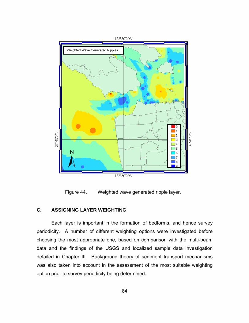
84

Figure 44. Weighted wave generated ripple layer.

C. ASSIGNING LAYER WEIGHTING

Each layer is important in the formation of bedforms, and hence survey

periodicity. A number of different weighting options were investigated before

choosing the most appropriate one, based on comparison with the multi-beam

data and the findings of the USGS and localized sample data investigation

detailed in Chapter III. Background theory of sediment transport mechanisms

was also taken into account in the assessment of the most suitable weighting

option prior to survey periodicity being determined.

Weighted Wave Generated Ripples

85

The layers were combined using the raster calculator tool, within the

spatial analyst application within ArcMap.

1. Option 1

Figure 45 shows the first option with the following weighting scheme:

weighted sediment size, 50%, weighted currents, 25% and weighted wave

generated ripples, 25%.

Higher combined weightings occur throughout the region of the Golden

Gate Channel, particularly in deeper water, the higher weightings extend offshore

from the channel. The region to the Northeast of the Golden Gate and the West

of the Alcatraz Shoal has the highest weighting. In this region the sediment size

was large, the currents were strong and the wave generated ripples were also

large.

86

Figure 45. Combined weighted layers, Option 1. 122°30'0"W

122°30'0"W

37°4

5'0"

N

37°4

5'0"

N

Option 1

87

2. Option 2

Figure 46 shows the second option, with equal weights employed:



Again the higher weightings occur to the Northeast of the Golden Gate

and the West of the Alcatraz Shoal. In this region the sediment size was large,

the currents were strong and the wave generated ripples were also large. There

is quite a high weighting offshore and also on the Northwest side of the channel.

This option has many regions with a low weighting, indicated by blue.

Figure 46. Combined weighted layers, Option 2.

122°30'0"W

122°30'0"W

37°4

5'0"

N

37°4

5'0"

N

Option 2

88

3. Option 3

Figure 47 shows the third weighting option, using the following weighting;



In this option higher priority is assigned to regions with strong current,

resulting in lower weightings over the majority of the area. Only the region to the

Northeast of the Golden Gate and the West of the Alcatraz Shoal would be

frequently surveyed, this would not capture all the dominant sand wave

movements.


122°30'0"W

122°30'0"W

37°4

5'0"

N

37°4

5'0"

N

Option 3

89

4. Option 4

Figure 48 shows the fourth weighting option, the following weighting was

employed; weighted sediment size, 25%, weighted currents, 25% and weighted

wave generated ripples, 50%.

From Figure 48, it can be seen that a large percentage of the region has a

weighting of 3. This indicates a relatively high changeability throughout the

area. Again the region to the Northeast of the Golden Gate and the West of the

Alcatraz Shoal stands out, as having the highest changeability. However, as the

magnitude of wave generated ripples appears to be much smaller than the effect

of sediment size and currents, this option should be immediately discounted.


122°30'0"W

122°30'0"W

37°4

5'0"

N

37°4

5'0"

N

Option 4

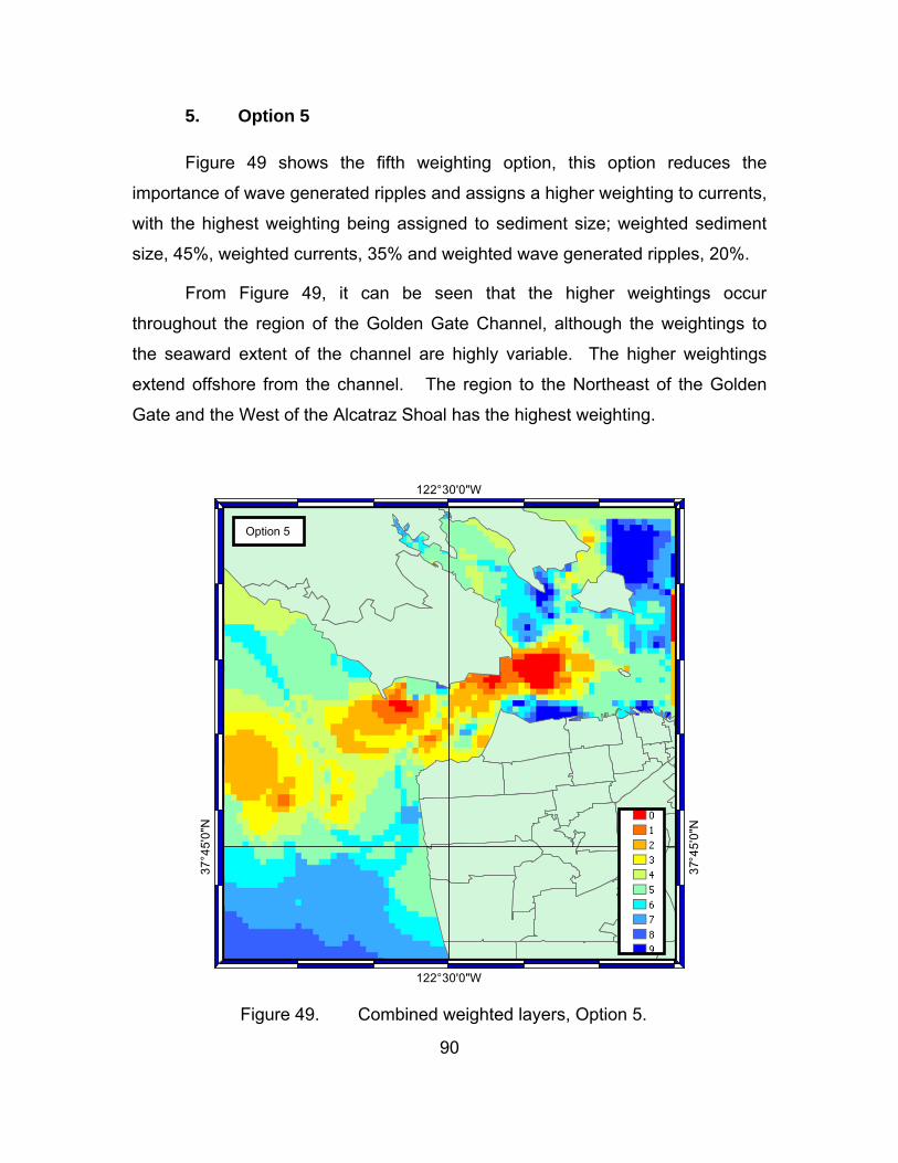
90

5. Option 5

Figure 49 shows the fifth weighting option, this option reduces the

importance of wave generated ripples and assigns a higher weighting to currents,

with the highest weighting being assigned to sediment size; weighted sediment

size, 45%, weighted currents, 35% and weighted wave generated ripples, 20%.

From Figure 49, it can be seen that the higher weightings occur

throughout the region of the Golden Gate Channel, although the weightings to

the seaward extent of the channel are highly variable. The higher weightings

extend offshore from the channel. The region to the Northeast of the Golden

Gate and the West of the Alcatraz Shoal has the highest weighting.


122°30'0"W

122°30'0"W

37°4

5'0"

N

37°4

5'0"

N

Option 5

91

D. DETERMINING SURVEY PERIODICITY

In order to determine the recommended survey periodicity, the weighted

option layers were reclassified, using the UKHO recommended re-survey

intervals (Table 3). This was achieved by reclassifying the layer into the four

survey categories. With category 1, indicating a high level of changeability and

therefore a low survey re-interval, shown in red. The lowest changeability,

category 4, was shown in blue.

From the detailed study of the five weighting options put forward in the

previous section, it was determined that Option 5 provided the best

representation of both the multi-beam data and the background theory.

Option 5 had 45% weighting for the sediment layer, from the background

theory it was extremely apparent that sediment grain size was particularly

important in sediment transport mechanisms and in bedform formation

mechanisms. Currents were weighted at 35%, this demonstrates the importance

of currents, in this case due to a particularly strong tidal regime, the importance

of currents was also apparent from the background theory of sediment transport.

Waves had a weighting of 20%, the lower weighting was due to the smaller

magnitude of ripple heights due to wave motion, although the ripple height from

wave motion cannot be discounted it is not of a large enough magnitude to cause

mine burial.

Each option was carefully compared to the known patterns of San

Francisco Bay from the high resolution USGS multi-beam data (Figures 23 to

27). Options 1 and 5 both showed a high correlation with this data. Options 2, 3

and 4, showed some correlation but it was significantly less than the other two

options. It was decided that Option 5 was the most representative; it captured

the majority of features shown on the multi-beam data.

The red regions of Figure 50, located throughout the Golden Gate

Channel and the Alkatraz Shoal, show the regions of highest seabed

changeability, those that should be surveyed most often. Following the UKHO

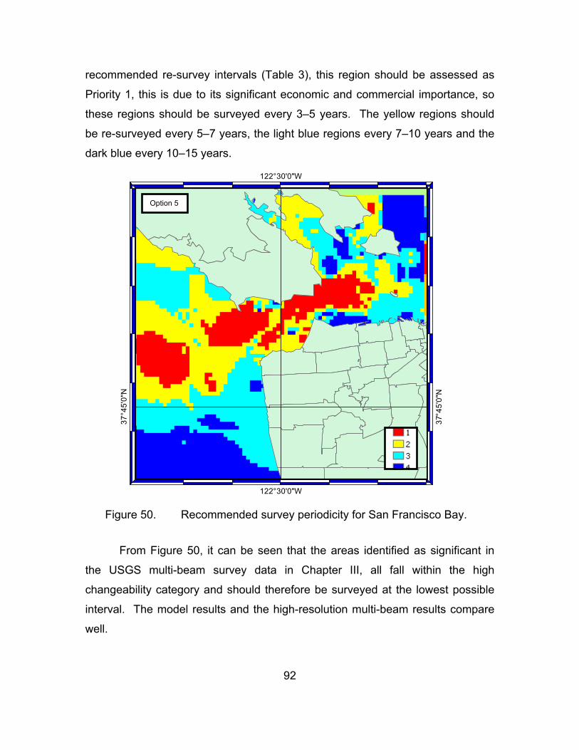
92

recommended re-survey intervals (Table 3), this region should be assessed as

Priority 1, this is due to its significant economic and commercial importance, so

these regions should be surveyed every 3–5 years. The yellow regions should

be re-surveyed every 5–7 years, the light blue regions every 7–10 years and the

dark blue every 10–15 years.

Figure 50. Recommended survey periodicity for San Francisco Bay.

From Figure 50, it can be seen that the areas identified as significant in

the USGS multi-beam survey data in Chapter III, all fall within the high

changeability category and should therefore be surveyed at the lowest possible

interval. The model results and the high-resolution multi-beam results compare

well.

122°30'0"W

122°30'0"W

37°4

5'0"

N

37°4

5'0"

N

Option 5

93

V. CONCLUSIONS AND RECOMMENDATIONS

It is essential to maintain an up-to-date database of route surveys for mine

warfare in order to maintain maritime security at home and abroad. Mine warfare

routes often pass through strategic sea-lanes in order to gain access to ports and

harbors, these routes traverse the littoral region, a complex oceanographic

environment, in which a variety of mines could be laid. This study is primarily

valid for VSW, SW and DW regions, not the surf zone as the sediment transport

mechanisms and processes are much more complex in this region. The

bathymetry in the regions of interest can be complex and often difficult to predict.

Complex bathymetry patterns hinder the mine warfare problem due to increased

clutter, scouring and burial of mines, unfortunately the impact of bathymetry,

particularly bedforms is poorly understood, and little research of the impact has

been conducted.

It is known that seabed type, sedimentation, and transport due to tides,

currents and wave interaction are extremely important in sediment transport

mechanisms and bedform formation. Sediment transport and bedform formation,

in turn, are extremely important in the mine warfare route periodicity problem,

when taking into account the size of a typical mine (height 0.5 m), a relatively

small change in ripple height or bedform height in any location can easily cause

the burial of a mine. By assessing the rate of change in a location an

assessment of survey periodicity can be made. Due to the complex nature and

number of mechanisms involved a qualitative rather than quantitative

assessment has been made.

The UKHO GIS weighted suitability model, formed a qualitative

assessment for the UK mine countermeasures route survey maintenance

schedule in 2005. This model could not be used for the U.S. due to its

geographic limitations, but the concepts used in its construction can. The U.S.

currently has no such model for determining route survey periodicity.

94

A. SUMMARY OF RESULTS

1. Localized Sample Data and Database Comparison Results

San Francisco Bay was used as a case study; a sediment analysis

investigation was carried out in February 2009. The investigation involved the

comparison of grab samples taken over a three-year period, the aim of this was

to determine if there had been any change with time in the sediment properties at

the sites sampled and to compare the results to the NAVOCEANO HFEVA

database, to assess if the database remained valid.

From the results it can be concluded that at the sites sampled, there was

not a significant change in sediment properties with time. From the results and

climatological data the predicted ripple heights were calculated, these results

concluded that the ripple heights showed variability of a few centimeters over the

three-year period, which is not deemed significant.

When compared to the NAVOCEANO HFEVA database the sediment type

of each sample concurred with the database results, suggesting that this

database remains a valid assessment of sediment type in this area. Every care

was taken to assure the accuracy of this investigation as discussed in Chapter III.

2. USGS Multi-beam Survey Results

The comprehensive results using high resolution multi-beam survey

techniques obtained by USGS show that bedform fields as a whole maintained

relative symmetry and asymmetry values had not changed markedly with time

(Barnard et al., 2007). From these results the temporal variability of bedforms in

the San Francisco Bay region was demonstrated.

The height of the bedforms was assessed as a significant factor in the

determination of route survey periodicity, as although the location of the bedform

fields did not change significantly with time, the location of the sand wave crests

95

did. This has the potential to cause mine burial and was of significant interest

during this study.

3. Modeling Results

The route survey periodicity model developed for San Francisco Bay was

based on the concepts of the UKHO model. Although different input layers were

used, the UKHO model included layers to depict the MCM environment and the

maritime environment, but did not include waves, tides or currents. Due to

difficulties sourcing the data included in the UKHO model for the San Francisco

Bay area an alternate approach was necessary. From background theory and

the experimental results it was apparent that bedform size and mechanisms were

an integral part of this problem. It was decided that sediment size, tides and

currents and ripples generated from wind waves were critical in bedform

formation and size. If this could be predicted, survey periodicity could be

determined based on the bedform size and the known movement characteristics.

The San Francisco model was comprised of three layers. The sediment

size layer was constructed from 174 grab samples, which were interpolated into

a raster dataset, from this predicted bedform type could be determined. Tides

and currents were accounted for by interpolating over 50 current stations. The

predicted wave generated ripple heights were calculated from climatological data

and the Wiberg and Harris model. Each layer was weighted, the weighting

scheme was used, and each layer was re-classified with a scale of 0 to 9, with 0

representing a high degree of change, and 9 representing little change. As these

layers had not been used before, the weighting schemes used were based

primarily on background theoretical concepts.

The recommended re-survey intervals, used in the UKHO model (shown

in Table 3) were used in this model. In order to determine the most

representative weighting of each layer, five options were examined. The

resulting layers were compared to the high-resolution multi-beam data, in order

to determine which weighting option was the most representative.

96

The fifth option had the predicted bedform type layer weighting of 45%, in

all background theory literature sediment size was shown to be the most

important factor in bedform type and hence size. The predicted bottom current

layer had a weighting of 35%, indicating that currents, in this case due to the tidal

regime had a greater importance than waves, which were given a weighting of

20%. A lower weighting was given to waves due to the fact that the ripple

heights capable of being generated were much smaller than those generated by

currents.

When compared to the high-resolution multi-beam data, this option was

deemed to be the most representative. In regions where the seabed

changeability was assessed to be high, a survey interval of 3–5 years was

assigned. A number of these regions corresponded with comprehensive regions

of study by the USGS (Figures 25–27). The temporal variability shown in these

regions indicate that this survey interval would be the most suitable. Figure 23

and 24; show the bed patterns in San Francisco Bay. When compared to the

model, the results are extremely encouraging.

B. RECOMMENDATIONS

This study has resulted in a number of recommendations. Potentially this

model could be used to determine the route re-survey interval for the US.

Implementing the three layers discussed could do this. The NAVOCEANO

HFEVA database could be used to form the basis of the predicted bedform layer.

However, it is recommended that NAVOCEANO include the recent grab sample

data obtained by USGS and other sources to improve the resolution of the

HFEVA database, this can be demonstrated by examination of Figures 22 and

32. This model could be used in other worldwide regions of interest as all the

input data can be gained from easily available open sources, although obviously

the better the resolution of the input data the better the results.

97

1. Recommendations for the UKHO Model

The San Francisco Bay model utilizes layers including; sediment size,

waves, tides and currents. One of the recommendations for areas of further

study in the UKHO 2005 report was to determine if any additional environmental

factors should be included in the model to refine the results. This investigation

has shown by using the three layers; sediment size, waves, tides and currents;

predicted bedform regions can be obtained and a survey periodicity determined.

Although the UKHO model does not include waves, tides and currents,

sediment type and bottom texture are included. Sediment size, waves, tides and

currents are the inputs required to determine bedforms. Bedforms are already

included in the UKHO model from sediment type and bottom texture. When

UKHO results are compared to results from the SEAs reports, it can be seen that

regions of bedforms, determined by the SEAs study, correspond to regions with a

low re-survey interval determined by the UKHO model. It is therefore,

recommended that inclusion of these extra environmental parameters is not

necessary for the UKHO model.

2. Limitations

In San Francisco Bay coarse sediments are found in regions of strong

tidal currents, this is where the larger bedforms occur. The same is true for

regions around the UK, however, this may not be true in all cases. A further

limitation could occur in regions of fine sediments, fine sediments would not

cause large ripple heights or bedforms to occur, however, they do remain a

region of interest for the mine warfare survey periodicity problem. In fine

sediment regions, a mine could potentially become buried by scour or suspended

sediments being washed down a river. This model does not capture these

effects.

98

3. Recommendations for Further Study

All results from this study indicate the San Francisco Bay model results

are viable and the survey periodicity suggested is credible for this area. It is

recommended that this study be replicated in a different regions, where high-

resolution multi-beam data is available and the weighting scheme for the model

verified by this.

Different regions should include regions with similar characteristics, for

example sandy sediments and strong tidal currents. If deemed correct then this

model could be implemented for use in the US and other similar regions of

interest. The model should also be replicated in regions of finer sediments to

determine if additional layers or and alternate weighting scheme should be used

in these regions.

From the results analyzed throughout this study, it has become apparent

that one of the most important factors in determining the survey periodicity for

mine warfare is sediment size, a further study could be conducted to determine if

an assessment of survey periodicity could be made from this data alone,

particularly in regions where little data is available.

99


100

LIST OF REFERENCES

Armishaw, J. E. (2005). Route Resurvey Model (QRM): Use of GIS Modelling to Review the UK Route Survey Maintenance Schedule. UKHO/MEIC TR/05/01, June 2005. Taunton, Somerset.

Armishaw, J. E. (2005). Optimising MW Surveying by Modelling the Seabed Environment using GIS Techniques. Adapted by DIJE from UKHO/MEIC TR/05/01, June 2005. Taunton, Somerset.

Bagnold, R. A. (1946). Motion of Waves in Shallow Water: Interaction Between Waves and Sand Bottoms. Proc. R. Soc. London Ser, A187, 1-15.

Bagnold, R. A. (1956). Flow of Cohesionless Grains in Fluids. Phil. Trans. Royal

Society, London, A249, 235-297. Barnard, P. L. et al. (2006). Giant Sand Waves at the Mouth of San Francisco

Bay. EOS, Vol 87, 29, 285-289. Barnard, P. L. et al. (2006). Massive Bedforms and their Movement Mapped at

the Mouth of San Francisco Bay Using Multibeam Sonar. American Geophysical Union, Fall Meeting 2006.

Barnard, P. L et al. (2007). Coastal Processes Study at Ocean Beach, San Francisco, California; Summary of Data Collection 2004-2006. US Geological Survey Open File Report 2007-1217. http://pubs.usgs.gov/of/2007/1217/

Barnard, P. L. et al, (In Press, 2009). Analyzing Bedforms Mapped Using

Multibeam�Sonar to Determine Regional Bedload Sediment Transport Patterns in�the San Francisco Bay Coastal System. Sedimentology, In: Li, M.,�Sherwood, C., and Hill, P. (Eds.), International Association of�Sedimentologist's Special Publication Book on Shelf Sedimentology, 33 pp.

Blondeaux, P. (2001). Mechanics of Coastal Forms. Annual Review Fluid

Mechanics, 33, 339–370.

British Geological Survey, (2005). DTI Strategic Enviromnetal Assessment Area 6, Irish Sea, Seabed and Surficial Geology and Processes. Continental Shelf and Margins Commissioned Report CR/05/057.

British Geological Survey, (2007). DTI Strategic Enviromnetal Assessment Area 8, Superficial Seabed Processes and Hydrocarbon Prospectivity. Marine Coastal and Hydrocarbons Commissioned Report CR/07/075.

101

California Department of Water Resources, (2007). Delta Outflow. California Data Exchange Center, http://cdec.water.ca.gov/

Clifton, H. E. (1976). Wave-formed Sedimentary Structures: A Conceptual

Model, in Beach and Nearshore Sedimentation. Edited by R.A. Davis and R. L. Ethington, SEPM Special Publication, 24, 126-148.

Dare, C; Craig, M and Torresan, M. (2006). Grain-Size Analysis of sediments

From San Francisco Bay: A Comparison of LISST and Sieve Analysis Methods. American Geophsical Union, Fall Meeting 2006.

Davis, A. G. et al. (2002). Intercomparision of Research and Practical Sand Transport Models. Coastal Engineering, 46, 1-23.

Deigaard, F. (1992). Mechanics of Coastal Sediment Transport. World Scientific, Singapore.

Dyre, K. R. (1986). Coastal and Estuarine Sediment Dynamics, John Wiley & Sons, Chichester.

Dyre, K. R. and Soulsby, R. L. (1988). Sand Transport on the Continental Shelf.

Annual Review Fluid Mechanics, 20, 295-324.

Fleet Numerical METOC Detachment, (2009). Marine Gridded Climatological Data: 1857-1997. Ashville. http://niprnavy.ncdc.noaa.gov/webv7-servlet/jsps/marine/context/idx_smgc_graphic.jsp

Friends of the Estuary, (1997). Annual Report, 1996-1997. Hudson, D. (2008). Sediment Analysis: Statistical Variation of Localized

Samples and Database Verification. OC3570: Operational Oceanography Report, Naval Postgraduate School, Monterey, California.

Hunt, J. N. (1979) Direct solution of wave dispersion equation. J. Waterways,

Ports, Coastal Ocean Div., ASCE 105(WW4):457-459. King, D. (2007). Sediment Analysis and Database Verification Report. OC3570:

Operational Oceanography Report, Naval Postgraduate School, Monterey, California.

Komar, P. D. (1976). Beach Processes and Sedimentation. Prentice-Hall, Inc.

New Jersey. Komar, P. D. and Reimers, C. E. (1978). Grain Shape Effects on Settling Rates.

Journal of Geology, 86, 193-209.

102

Liu, Z. (2001). Sediment Transport. Laboratoriet for Hydraulik og Havnebygning, Aalorg Universitet. http://lvov.weizmann.ac.il/lvov/Literature-Online/Literature/Books/2001_Sediment_Transport.pdf

MacVean, L. J. and Stacey, M. T. (2008). Lateral Mixing Processes in a Estuary:

San Francisco Bay and its Exchange With Perimeter Habitat. American Geophysical Union, Fall Meeting 2008.

McCave, I. N. (1971a). Wave effectivness at the Sea Bed and its Relationship to

bedforms and Deposition of Mud. Journal of Sedimentology and Petrolium, 41, 89-96.

McCave, I. N. (1971b). Sand waves of the North Sea off the Coast of Holland.

Marine Geology, 10, 199-225. McCoy, J. and Johnston, K. (2002). Using ArcGIS Spatial Analyst. ESRI.

Redlands, USA

Milliman, J. D. and Meade, R. H. (1983) World wide delivery of River Sediment to the Oceans. Journal of Geology, 91, 1-21.

National Research Council (2000): Oceanography and Mine Warfare. Ocean

Studies Board, Commission on Geosciences, Environment, and Resources. National Academy Press. Washington DC

National Research Council (2001). Naval Mine Warfare: Operational and Technical Challenges for Naval Forces. Committee for Mine Warfare Assessment, Naval Studies Board, www.nap.edu/catalog.php?record_id=10176

Parker, K. A. et al. (2003). Sediment Distribution in Central San Francisco Bay in the Vicinity of Racoon Strait. American Geophysical Union, Fall Meeting 2003.

Proudman Marine Laboratory (2009). Sediment Process Triad http://www.pol.ac.uk/home/research/theme3/wp33.php

Royal Navy (2004). BR1806: British Maritime Doctrine, 3rd Edition. Ministry of Defence, TSO (The Stationary Office). London

Royal Navy (2009). www.royalnavy.mod.uk/operations-and-support/surface-fleet/mine-countermeasure

Schoellhamer, D. H. (1996). Factors Affecting Suspended Solids Concentrations in South San Francisco Bay, California. Journal of Geophysical Research, Vol 101, C5, 12087-12096.

103

Sherwood, C. (2007). Demonstration Sediment Transport Applets. http://woodshole.er.usgs.gov/staffpages/csherwood/sedx_equations/sedxinfo.html

Stive, M. J. F. et al. (2002). Variability of Shore and Shoreline Evolution. Coastal Engineering, 47, 211-235.

Soulsby, R. L. et al. (1983). The Detailed Processes of Sediment Transport by Tidal Currents and by Surface Waves, Institute of Marine Sciences, Natural Environment Research Council. http://eprints.soton.ac.uk/14569/01/152.PDF

US Navy Marine Corps (2005). Mine Warfare. University Press of the Pacific, Honolulu, Hawaii

United States Army Corp of Engineers, (1996). Ocean Beach Storm Damage reduction Feasibility Study; Final Feasibility Study for the City and County of San Francisco. San Francisco District.

United States Naval Oceanographic Office. (September 2003). Database

Description for Surface Sediment Type, Stennis Space Center, Mississippi: Acoustics Division.

Weltmer, M. A. (2003). Bedform Evolution and Sediment Transport Under Breaking Waves. M.S. thesis, Naval Postgraduate School, Monterey, California.

Wiberg, P. L., and C. K. Harris (1994) Ripple geometry in wave-dominated

environments. Journal of Geophysical Research, 99(C1):775-789

Wikipedia, (2009). Naval Mine. http://en.wikipedia.org/wiki/Naval_mine

Wikipedia, (2009). Sediment Transport. http://en.wikipedia.org/wiki/Sediment_transport

104

INITIAL DISTRIBUTION LIST

1. Defense Technical Information Center Ft. Belvoir, Virginia

2. Dudley Knox Library Naval Postgraduate School Monterey, California

3. Professor Peter Chu Department of Oceanography Naval Postgraduate School Monterey, California

4. Professor Thomas Herbers

Department of Oceanography Naval Postgraduate School Monterey, California

5. Dr J E Armishaw

Maritime Environment Information Centre Hydrographic Office Admiralty way Taunton Somerset TA1 2DN United Kingdom

6. Dr Patrick Barnard Research Geologist USGS Pacific Science Center 400 Natural Bridges Drive Santa Cruz, California

7. Lt Cdr C Chapple RN SO2 ENVIRON

Maritime Warfare Centre Room F190, Marlbourough Building HMS Collingwood Newgate Lane, Fareham Hampshire, PO14 1AS United Kingdom

105

8. Lt Cdr K Pullen RN DI ICSP-JGI-HM1-SO2

DI ICSP Old War Office Whitehall London SW1A 2EU United Kingdom

9. Cdr M Jones RN

CDR HM Room 225 Defiance Building HMNB Devonport Plymouth Devon, PL2 2BG

10. Cdr A V Swain RN FOST HM

Fitzroy Building Upper Battery Road HMNB Devonport Plymouth Devon, PL2 2BG United Kingdom

11. Cdr D Turner RN British Embassy Washington DC, 20008

Documents

NAVAL POSTGRADUATE SCHOOL - oc.nps.educhu/web_paper/thesis/wheatley.pdf · naval postgraduate school monterey, california ... mine warfare: investigation of bedforms, waves, tides,