NAVAL POSTGRADUATE SCHOOL Monterey, California · file cvi naval postgraduate school monterey, california 0, thesis analysis of the accuracy of a propossed target motion analysis

FILE CVI

NAVAL POSTGRADUATE SCHOOLMonterey, California

0,

THESIS

ANALYSIS OF THE ACCURACY OF APROPOSSED

TARGET MOTION ANALYSIS PROCEDURE

by

Bernabe Carrero Cuberos

1989 September

Thesis Advisor James N. EagleCo-Advisor Donald P. Gaver

Approved for public release; distribution is unlimited

DTIC/ " Iii - AMAR 16 1990

Unclassifiedsecurity classification of this page

REPORT DOCUMENTATION PAGEI a Report Security Classification Unclassified lb Restrictive Markings

2a Security Classification Authority 3 DstributionAvailability of Report2b Declassification Downgrading Schedule Approved for public release; distribution is unlimited..1 Performing Organization Report Numbcr(s) 5 Monitoring Organization Report Number(s)

6a Name of Performing Organization 6b Office Symbol 7a Name of Monitoring OrganizationNaval Postgaduate School (if app'"abte) 55 Naval Postgraduate School6c Address (elry, state, and ZIP code) 7b Address (city, state, and ZIP code)Monterey, CA 93943-5000 Monterey, CA 93943-5000Sa Name of Funding Sponsoring Organization 8b Office Symbol 9 Procurement Instrument Identification Number

(I applicable)Sc Address (city, state, and ZIP code) 10 Source of Funding Numbers

Program Element No I Project No I Task No I Work Unit Accession No

11 Title (Incl.de security classification) ANALYSIS OF THE ACCURACY OF A PROPUS ED TARGET MOTION ANALY-SIS PROCEDURE12 Personal Author(s) Bernabe Carrero Cuberos )g13a Type of Report 13b Time Covered 14 Date of Report (year, month, day) 15 Page CountMaster's Thesis From To 1989 September 6616 Supplementary Notation "lhe views expressed in this thesis are those of the author and do not reflect the official policy or po-sition of the Department of Defense or the U.S. Government.1"7 Cosati Codec 1S Subject Terms (contlnue on reverse if necessary and Identify by-block number)Field Group Subgroup TMA, Passive bearings-only.

Abstract (continue on reverse if necessary and ldenty by block number)T]is thesis inestigates the accuracy of a recently proposed passive bearings-only Target Motion Analysis (TMA) proce-

dure. The primary method of analy .is is to compare computer generated positions of a Target that is moving with a constantcourse and speed, with the procedurally derived estimated positions.

A computer model i as de% eloped \ hich simulated several possible interactions -between the Target and Own Ship. Es-timated parameters of the Target track % ere computed using the procedure under analysis. These values were compared tothe "true" values generated by the simulation.

An anal\ sis of the TMA procedure as originally proposed sho\%ed that it failed to accurately estimate the target track pa-rameters. However \ ith some modifications, the accuracy improved significantly and it is felt that the procedure can accu-rately estimate target range (but not necessarily course and speed) for some target geometries.

20 Distribution Availability of Abstract 21 Abstract Security Classification_0 unclassificd unlimited 1 same as report 0] DrIC users U'classified22a Name of Responsible Individual 22b Telephone (include Area code) 22c Office SymbolJames N. Fagle (408) 646-2654 155ErDD FORM 1473,84 MAR 83 APR edition may be used until exhausted security classification of this-page

All other editions are obsolete

Unclassified

Approved for public release; distribution is unlimited.

Analysis of the Accuracy of aPropossed

Target Motion Analysis Procedure

by

Bernabe Carrero Cuberos

Commander, Venezuelan NavyB.S., Venezuelan Naval School., 1985

Submitted in partial fulfillment of the

requirements for the degree of

MASTER OF SCIENCE IN OPERATIONS RESEARCH

from the

NAVAL POSTGRADUATE SCHOOL

1989 September

Author:

e abe Carrero Cuberos

Approved by: xJames N. Eagle, Thesis Advisor

Donald P. Ga , Co-Advisor

Peter Purdue, Chairman,Department of Operations Research

ii

ABSTRACT

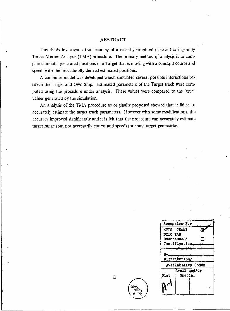
This thesis investigates the accuracy of a recently proposed rassive bearings-only

Target Motioln Analysis (TMA) procedure. The primary met hod of analysis is-to, c6m-

pare computer generated positions of a Target that is moving with a constant course and

speed, with the procedurally derived estimated positions.

A computer model was developed which simulated several possible interactions-be-

tween the Target and Own Ship. Estimated parameters of the Target track were com-

puted using the procedure under analysis. These values were compared to the "true"

values generated by the simulation.

An analysis of the TMA procedure as originally proposed showed that it failed to

accurately estimate the target track parameters. However with some modifications, the

accuracy improved significantly and it is felt that the procedure can accurately estimate

target range (but not necessarily course and speed) for some target geometries.

Accessio-n ForNITIS -GRA&IDTIC TAB 0

Just if-19atioL

Distribution/Availabi-lity Codes

Avail and/or:Dist Special

TABLE OF CONTENTS

I. INTRODUCTION TO THE PASSIVE RANGING PROBLEM ............ 1A. BRIEF HISTORY ........................................... 1B. PURPOSE OF THE THESIS ................................... 2

C. PROBLEM DESCRIPTION ..................................... 3

D. ASSUMPTIONS FOR THE SIMULATION ....................... 5

E. TERMINOLOGY .......................................... 5

II. TESTING THE BEARING EXTRAPOLATION PROCEDURE .......... 7

A. INITIAL CONDITIONS ...................................... 7

B. DESCRIPTION OF THE SIMULATION ......................... 7

C. TESTING THE BEARING EXTRAPOLATION PROCEDURE UNDERIDEAL CONDITIONS .......................................... 8

D. TESTING WITH BEARING ERRORS .......................... 12

E. ANALYSIS OF TIHE RESULTS ............................... 15

1. Differences Between Lead-Leg and Lag-Leg-Estimation ............ 15

2. Explanatiorn of Why Lag-Leg Estimation is Better than Lead-Leg Esti-m ation ...... ... ... ... ...... ... ... ..................... ...... 17

F. CONCLUSIONS ........................................... 20

-I11. POSSIBLE IMPROVEMENTS, AND ANALYSIS OF THEIR ACCURA-

C IE S .... .... .... ..... .. ........ ............... ... ...... ... ... 21

A MINORCHANGES ....................................... 21

1. Increase in Leg Length .................................... 21

2. Use of a Quadratic Model-to Fair the Lag-Leg .................. 21

3. Increase in Turn Time .................................... 21

B-. ELIMINATION OFI TJ-KE LEAD-LEGEST[MATION .............. 221. W ithout M inor Changes ................................... 23

2. With Increascd Leg, Length and Lag-Leg Faired with a Quadratic Model, 233. W;th =rv,,,, .' o ,",i, P=us an crease in Tur'n Duration .... 26

a. Effect of Target Courses Greater than 1,500 when Lag-Leg Esti-

mation and Mino0 Changes are Used ............................... 28

jirv

C. USE OF AN ARCTANGENT MODEL TO EXTRAPOLATE THE

LAG-LEG BEARINGS ........................................ 30

1. Fitting the Arctangent Model by Using Least Squares ............. 31

2. Estimation of the Parameters for the Arctangent Model by Solving a

System of Linear Equations ...................................... 33

IV. CONCLUSIONS AND RECOMMENDATIONS .................... 37

I. CONCLUSION S ........................................ 37

2. RECOMMENDATIONS ................................. 37

APPENDIX A. DISCUSSION OF SELECTED SOLUTION METHODS ..... 38

A. SPIESS RANGING ......................................... 38

B. EKELUND RANGING ...................................... 38

C. CHURN M ETHOD ......................................... 41

APPENDIX B. VARIABLES OF THE SIMULATION PROGRAM ......... 42

APPENDIX C. SIMULATION PROGRAM CODE ..................... 46

LIST OF REFERENCES .......................................... 57

INITIAL DISTRIBUTION LIST .................................... 58

I:V

S--- - - - --!:--------- - - - - - - - - - - - -

ACKNOLEDGEMENTS

I would like to express my gratitude to Prof. James N. Eagle and to Prof. Donald

P. Gaver for their assistance, guidance, and encouragement which they provided during

the pursuit of this work.

A special note of thanks is extended to LCDR. William Walsh, CPT. Charles H.

Shaw, III, and LT. Scott Negus for their help in the revision of the formal English

needed for this work.

I also want to dedicate my work to my lovely wife Tahamara and to my sons Sandy

Gabriel, Daniel Antonio, and Jenny Coralis for their patience, understanding and

fortitude given to me during my studies at the Naval Postgraduate School.

vi

I. INTRODUCTION TO THE PASSIVE RANGING PROBLEM

A. BRIEF HISTORYThe importance of doing Target Motion Analysis (TMA)I by a passive bearings-

only tracking technique has had the attention of many tacticians over the last 45 years,

mainly because the submarine's objective is to remain covert (undetected) during the

tracking maneuver. This guarantees the advantage of surprise if an attack is to be per-

formed.

In the early part of WWII, TMA by passive bearings-only methods began to be

used, and the following drawn from Naval Tactical Decision Aids by D. H. Wagner, 1989,

provides a brief history of its development:

During WWII LT. F. C. Linch developed the Linch Plot, which uses a pivotalrelationship among bearings, bearing rate, and Target relative motion. Based onthat, he developed a graphical method that was used until the late 1960's. It wasabandoned -because it was useful only for the short ranges contemplated by Linchat that time.

During the 1950's, various human plot methods and nomographs were used forTMA. One of the oldest of these was the Strip Plot, later called Geographical Plot.This method has often been used to provide upper and lower bounds on Targetrange. based on bounds on speed. An additional much used nomographic devicehas been the Bearing Rate Slide Rule. An early TMA computer was the PositionKeeper, which was a carryover from WWII, and used as an aid to approach andattack surface ships.

In 1953, F. N. Spiess published a graphical procedure requiring four bearings anda maneuver by Own Ship. This method is known as Spiess Plot. It remains in usein surface ship TMA.

The 1954 command thesis of LT. J. F. Fagan derived a four-bearing TMA sol-ution. which was a transcendental system of three equations with three unknowns.To reduce to computability by slide rule, he assumed that Own Ship motion duringthe first three bearings was approximately zero which was probably satisfactory fordiesel operations.

In 1957, LT. .. J. Ekelund devised one of the most famous TMA methods, nowcalled Ekelund Ranging.

Between 1967 and 1969, D. C. Bossard with a group of USN officers, made ananai sis of the fundamentals of bearings-only ranging and the effect of Own Ship

I Determination of Target range. course, and speed

maneuvers on ranging accuracy. Through this work and trials at sea, -they observedthat ranging errors could be eliminated by judicious choice of the time- for which therange was estimated. Also, by selecting some particular maneuvers, this best timecould be controlled to be in the past, present, or future; then they applied thismethod to various forms of bearings-only ranging, especially to Ekelund and Spiessmethods. The general name for these procedures is Time Correction.

In August 1968, a series of exercises was conducted aboard the USS Pargo tocompare the different methods in use at that time. The Passive Ranging Manualevolved in three volumes from the report of the analysis of these exercises and waspublished later as an NWP. This is a basic reference today for TMA.

In the late 1960's the CHURN method appeared, which uses a large number ofbearing observations and regression methods to do TMA. This method was devel-oped by General Dynamics: Electric Boat and Librascope.

In 1969, H. W. Headle, J. Di Russo, and E. Messere developed the ManualAdaptive TMA Evaluator (MATE). This method begins with an input estimate ofTarget course, speed and range, and from there estimated bearings are computedand compared against observed bearings. Differences between these bearing valuesare plotted against time. If these differences are distributed roughly symmetricallyas white noise about zero, while Own Ship changes course or speed, then the trialsolution is a good one; otherwise the MATE operator adjusts the input Target pa-rameters.

In the early 1970's, the application of Kalman filtering appeared for the-first timein TMA. It was a done by J. S. -Davis of NUSC, based on the Ph. D. thesis of D.J. Murphy at Northeastern University. Later versions were developed-by -IBM.

In the mid 1970's,-a new TMA method known as FLIT was devised by ENS. L.Anderson which has seen considerable effective operational use. Its methodologyremains classified.

In the mid and later 1970's, ranging and tracking at long range on-a sphere weredeveloped by D. C. Bossard, J. B. Behrla, and L. K. Graves of Daniel -H. Wagner,Associates. This was motivated by over-the-horizon targeting needs.

In the late 1970's and during the 1980's, further developments were made by usingKalman filtering and also-stochastic differential equations. The Maneuvering TargetStatistical Tracker (MTST)-is a method devised from this basis by W. H. Barker ofDaniel H.Wagner, Associates.

From 1985 to 19S7 the -Generical Statistical Tracker (GST) was developed atDaniel H. Wagner, Associates. This is a PC version of MTST.

B. PURPOSE OF THETHESiS

In late 19S8, LCDR P. K. Peppe of the USS La Jolla (SSN 701) -proposed a

bearing-only Target Motion Analhsis (TMA) procedure (here called the Bearings Ex-

trapolation Procedure) for use in submarines [Ref. I]. It is the purpose of this thesis to

test the accuracy of this procedure against a nonmaneuvering Target.

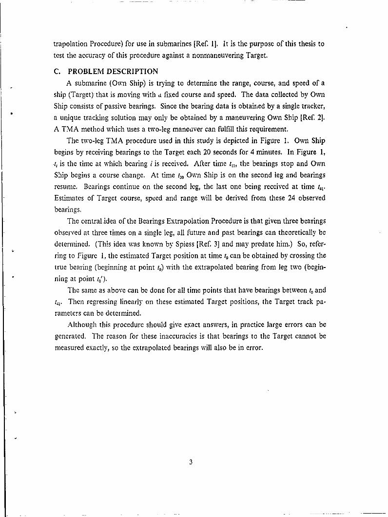
C. PROBLEM DESCRIPTION

A submarine (Own Ship) is trying to determine the range, course, and speed of a

ship (Target) that is moving with t fixed course and speed. The data collected by Own

Ship consists of passive bearings. Since the bearing data is obtained by a single tracker,

a unique tracking solution may only be obtained by a maneuvering Own Ship [Ref. 2].

A TMA method which uses a two-leg maneuver can fulfill this requirement.

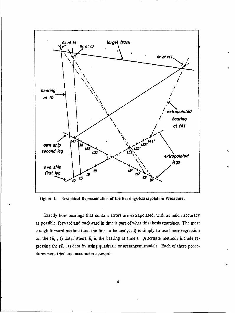
The two-leg TMA procedure used in this study is depicted in Figure 1. Own Ship

begins by receiving bearings to the Target each 20 seconds for 4 minutes. In Figure 1,

-t, is the time at which bearing i is received. After time t,, the bearings stop and Own

Ship begins a course change. At time t30 Own Ship is on the second leg and bearingsresume. Bearings continue on the second leg, the last one being received at time t4,.

Estimates of Target course, speed and range will be derived from these 24 observed

bearings.

The central-idea of the Bearings Extrapolation Procedure is that given three bearings

observed at three times on a single leg, all future and past bearings can theoretically be

determined. (This idea was known by Spiess [Ref. 3] and may predate him.) So, refer-

ring to Figure 1, the estimated Target position at time to can be obtained by crossing the

true bearing (beginning at point to) with the extrapolated bearing from leg two (begin-

ning at point to').

The same as-above can be done for all time points that have bearings between t, and

t,,. Then regressing linearly on these estimated Target positions, the Target track pa-

rameters can be determined.

Although this procedure should give exact answers, in practice large errors can be

generated. The reason for these inaccuracies is that bearings to the Target cannot be

measured exactly, so the extrapolated bearings will also be in error.

I3

fix at 0 target track

• ~fix at Ml I

~/"

own shipsecond leg t

extraplated

own ship

fiarstng "s N

Figure 1. Graphical Representation of the Bearings Extrapolation Procedure.

Exactly how-bearings that contain errors are extrapolated, with as much accuracy

as possible, forward-and backward in time is part of what this thesis examines. The most

straightforward -method (and the first to be analyzed)-is simply to use linear regression

on the (B, , t) data,where B, is the bearing at time -t. Alternate methods include re-

gressing the (B,-, Q) data by using quadratic or arctangent-models, Each of these proce-

dures were tried and-accuracies assessed.

4

The Spiess Graphical Method, Ekelund Ranging, and the CHURN Method are

closely related to the procedure proposed by Peppe, and for that reason they are further

explained in Appendix A

D. ASSUMPTIONS FOR THE SIMULATION

The computer simulation used in this study uses the following assumptions:

1. The Target moves at a constant course and speed throughout the tracking maneu-'er.

2. Differences in depth for the Target and Own Ship are disregarded.

3. Errors in position for Own Ship are disregarded.

4. Errors in bearings to the Target are independent and identically distributed normalrandom variables with mean zero and standard deviation not larger than 1.50. Inaddition, this standard deviation is constant for each simulation experiment.

5. Bearings to the Target are obtained each 20 seconds.

6. Initial course, speed and range for the Target and initial course and speed for OwnShip are as described in Chapter II.

E. TERMINOLOGY

1. Lead-leg. An Own Ship course such that Own Ship speed across the line of soundis in the same direction as the Target speed across the line of sound at the start oftile leg.

2. Lag-leg. An Own Ship course such that Own Ship speed across the line of soundis in the opposite direction to the Target speed across the line of sound at the startof the leg.

3. Leg length. The distance along either leg where bearings are received (does notinclude Own Ship turn).

4. Raw bearing. An unsmoothed bearing to the Target.

5. Faired bearing. A bearing obtained after smoothing of the raw bearings.

6. Extrapolated positions. Positions of Own Ship obtained by extending the first legforward'in time or the second leg backward in time.

7. Extrapolated bearings. Bearings obtained by extrapolating actual bearings forwardin time for-the first leg or backward in time for the second leg.

S. Lead-le, estimation. The estimated target track obtained by linear regression ofestimated Target positions. These estimated Target positions are obtained from theintersection of faired bearings from the lead-leg and extrapolated bearings from thelag-leg.

9. ta2-ie. estimation The estimated target track obtained by linear regression ofestimated Target positions. These estimated Target positions are obtained from theintersection of faired bearings from the lag-leg and extrapolated bearings from thelead-leg.

10. Lead angle. Angle between the line of sound and the course of Own Ship when-itis leading the Target.

11. La2 angle. The angle between the line of sound and the course of Own Ship whenit is lagging the Target.

12. Angle on the bow. The angle between the line of sound and the course of theTarget.

6

II. TESTING THE BEARING EXTRAPOLATION PROCEDURE

A. INITIAL CONDITIONSIn order to perform a thorough analysis of the Bearing Extrapolation Procedure,

5,184 separate simulation experiments were conducted. Each experiment used one of thepossible combinations of the following parameters:

1. The initial Target positions were all due north from Own Ship (i. e., 0000) at oneof three different initial distances: large (= 60,000 yds), medium (= 30,000 yds),and short (= 10,000 yds).

2. Six courses for the Target were used: 0300, 0600, 0900, 1200, 150', and 1750.

3. Three speeds for the Target: 25, 15, and 5 knots.

4. Four courses for Owin Ship in the lead-leg: 060', 0700. .:800, and 0900.

5. Four courses for Own Ship in the lag-leg: 2700, 2800, 2900, and 3000.

6. Three speeds for Own Ship: 5, 10, and 15 knots.

7. Two maneuvers by Own Ship: lead-lag and lag-lead.

8. Four bearing error standard deviations: 0', 0.50 , 1, and 1.50.

It is important to mention that because of problem symmetry and the fact that both

lead-lag and lag-lead maneuvers are simulated, there was no need for simulating coursesfor the Target from 1800 to 3600.

The randomness in the simulation was introduced only through errors in the re-ceived -bearings.

B. DESCRIPTION OF THE SIMULATION

The simulation was written in Fortran 77 [Ref. 4] and executed on an IBM 3033

mainframe. Appendix B has a complete listing of all variables of the simulation pro-gram. Appendix C is a listing of the simulation progiam code.

For each combination of initial conditions, the simulation was repeated 100 times

with different seeds for pseudorandom-generation of bearing error. For each of the re-petitions. the following steps were conducted:

1. Target positions were simulated every 20 seconds for the entire maneuver.

. For the first leg the folio uwn-data was generated:

a. Own-Ship position every 20 seconds.

b. Bearing to the Target every 20 seconds (normal errors are added).

7

c. Own Ship track extended beyond the turn.

3. For the first leg the following data was then computed:

a. Coefficients for linear and quadratic fits for bearings versus time.

b. Faired bearings and extrapolated bearings using the results from linear orquadratic fit.

4. Own Ship course was determined for the second leg; based on the required secondleg. lead or lag angle, and the line of sound specified by the extrapolated bearingat the middle of the maneuver (t20).

5. Simulations and computations for the second leg were completed in the samefashion.

6. Estimated positions of the Target in two coordinates (X and Y) were computed bydetermining the point of intersection of faired bearings with their correspondingextrapolated- bearings.

7. Linear and orthogonal regression is conducted on the estimated Target positions(in X versus Y c-)ordinates), to determine the Target course.

S. Range to the Target at the end of the maneuver was obtained by computing thedistance between Own Ship's actual position at -the end of the second leg and theestimated Target position.

9. Finally. Target speed was obtained by computing the distance between the esti-mated Target -position at time to and the estimated Target position at the end of thesecond leg (t,,), on the fitted Target track, and then dividing this distance by141 -t10

The simulation of the bearine errors was done using the Linear CongruentialMethod for uniform pseudorandom numbers, combined with the Box and Muller

Method to produce normal variates [Refs. 5,6]. These procedures were selected to allow

-the simulation to be pc:rformed on a- personal computer.

C. TESTING THE BEARING EXTRAPOLATION PROCEDURE UNDER IDEALCONDITIONS

Here bearings to the Target were considered without error. Also the bearing rates-immediately before the turn (used to extrapolate bearings forward in time) and imme-

diately after the turn (used to extrapolate bearings backward in time) were computed

exactly with no errors introduced. The only source of error in this case was the linear

bearing extrapolation. This case is intended to be an-optimistic bound on the accuracyof the bearing extrapolation procedure when linear regression is used.

The ineasuie of effectiveness -(MOE) for the accuracy of this procedure was thepercentage of times that the estimated error was within 10% for range, 200 for course,

and 10% for speed from the actual-parameters of the Target track. These results are

8

presented in Table I and Table 2 for lead-lag and lag-lead maneuvers respectively.

Each number in these Tables resulted from the examination of 18 simulation exper-iments (six Target courses and three Target speeds). For example, when the initial dis-

tance was large, lead and lag angles 70% and Own Ship speed 15 knts, then five of the

18 simulations experiments (or 27.8%) resulted in the calculated Target speed beingwithin 10% of the actual Target speed. Note that without bearing error, the simulation

experiments are deterministic.

9

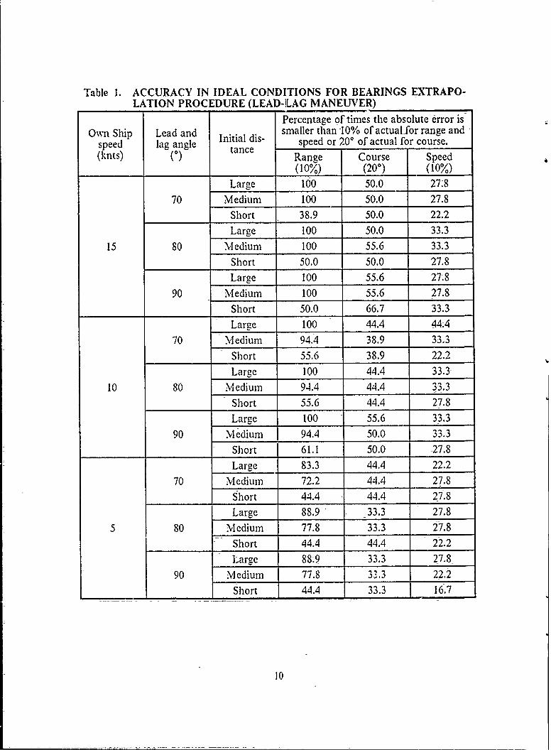
Table 1. ACCURACY IN IDEAL CONDITIONS FOR BEARINGS EXTRAPO-

LATION PROCEDURE (LEAD-LAG MANEUVER)

Percentage of times the absolute error isOwn Ship Lead and Initial dis- smaller than 10% of actual-for range and

speed lag angle tance speed or 200 of actual for course.(knts) (0) Range Course Speed

(10%) (200) (10%)Large 100 50.0 27.8

70 Medium 100 50.0 27.8

Short 38.9 50.0 22.2

Large 100 50.0 33.3

15 80 Medium 100 55.6 33.3

Short 50.0 50.0 27.8

Large 100 55.6 27.8

90 Medium 100 55.6 27.8

Short 50.0 66.7 33.3

Large 100 44.4 444

70 Medium 94.4 38.9 33.3

Short 55.6 38.9 22.2

Large 100 44.4 33.3

10 80 Medium 94.4 44.4 33.3

Short 55.6 44.4 27.8

Large 100 55.6 33.3

90 Medium 94.4 50.0 33.3

Short 61.1 50.0 27.8

Large 83.3 44.4 22.2

70 Medium 72.2 44.4 27.8

Short 44.4 44.4 27.8

Large 88.9 33.3 27.8

5 80 Medium 77.8 33.3 27.8

Short 44.4 44.4 22.2

Large 88.9 33.3 27.8

90 Medium 77.8 33.3 22.2

Short 44.4 33.3 16.7

10

Table 2. ACCURACY IN IDEAL CONDITIONS FOR BEARINGS EXTRAPO-LATION PROCEDURE (LAG-LEAD MANEUVER)

Percentage of times the absolute -error isOwn Ship Lead and initial dis- smaller than 10% of actual for range and

speed lag angle tance speed or 200 of actual for course.(knts) (0) Range Course Speed

(10%) (20°) (10%)Large 88.9 77.8 27.8

70 Medium 66.7 77.8 27.8Short 50.0 50.0 33.3Large 88.9 94.4 38.9

15 80 Medium 72.2 88.9 50.0

Short 50.0 33.3 33.3Large 94.4 94.4 44.4

90 Medium 72.2 88.9 44.4Short 38.9 27.8 27.8Large 83.3 88.9 22.2

70 Medium 66.7 94.4 22.2

Short 44.4 50.0 27.8

Large 83.3 94.4 33.310 80 Medium 61.1 88.8 33.3

Short 50.0 44.4 22.2Large 77.8 94.4 38.9

90 Medium 61.1 88.9 38.9Short 50.0 38.9 16.7

Large 72.2 77.8 33.370 Medium 50.0 77.8 27.8

Short 38.9 66.7 27.8

Large 72.2 77.8 33.35 80 Medium 50.0 77.8 27.8

Short 44.4 66.7 27.8Large 72.2 77.8 38,9

90 Medium 50.0 77.8 33.3

Short 44.4 66.7 22.2

11

As can be seen in Table 1 and Table 2, the following results were ob.,"d under

ideal conditions:

1. Range estimation is good, but only for medium or large initial distances.

2. Accuracy improves with increases in Own Ship speed.

3. Course and speed estimation is less accurate than range estimation.

4. Accuracy improves with increases in lead and lag angle.

5. Lead-lag maneuvers give better range estimates than do lag-lead, but not neces-sarily better course-and speed estimates.

It is felt that the procedure performed poorly for short initial- distances, in part be-

cause the bearing versus time curve is more nonlinear in -this case.

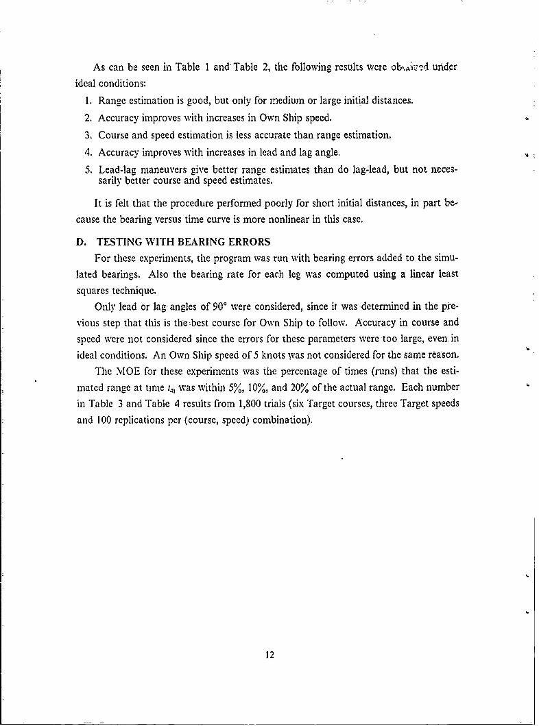
D. TESTING WITH BEARING ERRORS

For these experiments, the program was run with bearing errors added to the simu-

lated bearings. Also the bearing rate for each leg was computed using a linear least

squares technique.

Only lead or lag angles of 90* were considered, since it was -determined in the pre-

vious step that this is the best course for Own Ship to follow. Accuracy in course and

speed were not considered since the errors for these parameters weretoo large, even in

ideal conditions. An Own Ship speed of 5 knots was not considered for the same reason.

The NIOE for these experiments was the percentage of times (runs) that the esti-

mated range at time t,, was within 5%, 10%, and 20% of the actual range. Each number

in Table 3 and Table 4-results from 1,800 trials (six Target courses, three Target speeds

and 100 replications per (course, speed) combination).

12

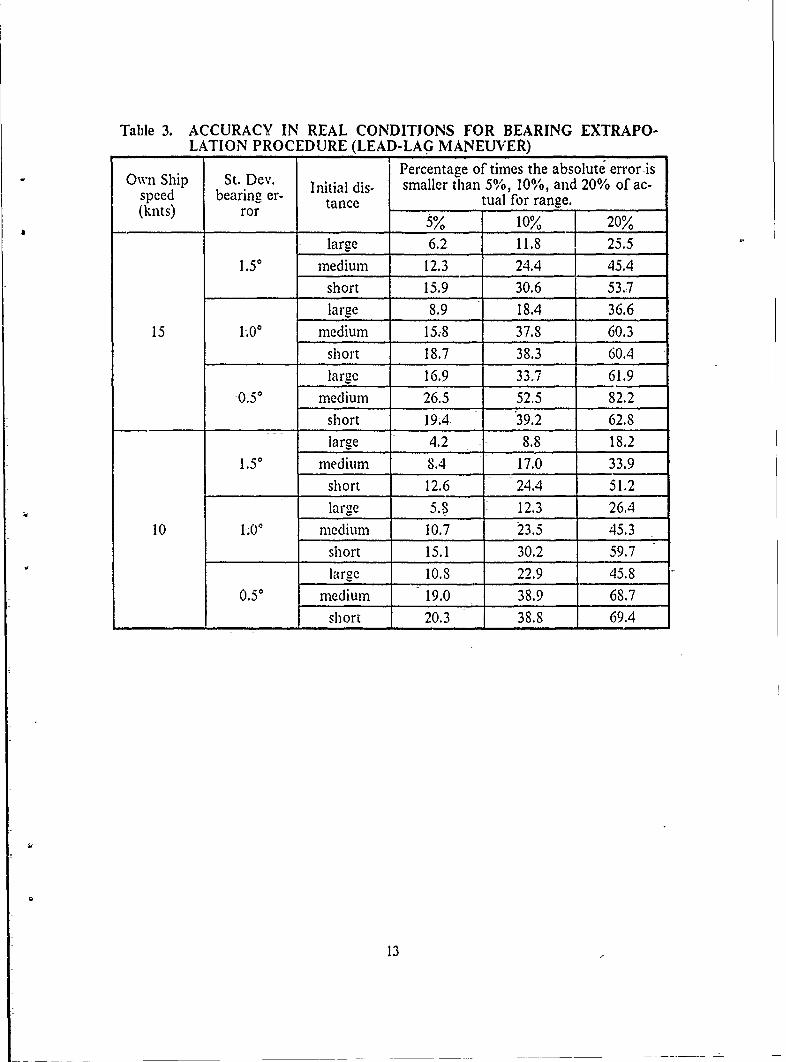
Table 3. ACCURACY IN REAL CONDITJONS FOR BEARING EXTRAPO-LATION PROCEDURE (LEAD-LAG MANEUVER)

Percentage of times the absolute error isOwn Ship St. Dev. Initial dis- smaller than 5%, 10%, and 20% of ac-

specd bearing er- tance tual for range.(knts) ror20

large 6.2 11.8 25.51.50 medium 12.3 24.4 45.4

short 15.9 30.6 53.7large 8.9 18.4 36.6

15 01,0 medium 15.8 37.8 60.3short 18.7 3S.3 60.4

large 16.9 33,7 61.90.50 medium 26.5 52.5 82.2

short 19.4 39.2 62.8large 4.2 8.8 18.2

1.50 medium 8.4 17.0 33.9

short 12.6 24.4 51.2

large 5.8 12.3 26.4

10 1.01 medium 10.7 23.5 45.3short 15.1 30.2 59.7large 10.8 22.9 45.8

0.50 medium 19.0 38.9 68.7

short 20.3 38.8 69.4

13

Table 4. ACCURACY IN REAL CONDITIONS FOR BEARING EXTRAPO-LATION PROCEDURE (LAG-LEAD MANEUVER)

Own Ship St. Dv. itPercentage of times the absolute error isOsip ba Der- Initial dis- smaller than 5%, 10%, and 20% of ac-speed bearing r- tance tual for range.(knts) ror 5% 10% 20%

large 4.7 11.3 23.2

1.50 medium 10.3 19.7 36.5short 6.7 12.3 23.9large 7.11 15.9 34.3

15 1.00 medium 11.7 24.2 46.6

short 6.7 12.2 22.2large 16.2 31.8 56.1

0.50 medium 17.1 30.9 54.9

short 5.3 11.6 21.4

large 4.0 7.4 18.1

1.50 medium 7.3 13.7 26.9

short 5.7 11.7 21.9large 5.4 10.8 23.4

10 1.00 medium 9.0 17.3 35.9short 5.0 10.8 23.2

large 11.0 22.2 42.90.50 medium 12.4 25.1 46.2

short 3.8 9.7 23.6

From Table 3 and Table 4, the following results are obtained:

1. The higher the Own Ship speed, the better the accuracy.

2. The best accuracy is obtained for medium initial distances.

3. The smaller the-bearing error, the better the accuracy.

4. A lead-lag maneuver gives better accuracy than lag-lead maneuver.

It is noted that orthogonal regression was also tried on the estimated Target posi-

tions, but with results similar to -those obtained with linear -egression. Subsequent ex-

periments used only linear regression.

14

E. ANALYSIS OF THE RESULTS

It appears that even in the absence of bearing errors, the Bearing Extrapolation

Procedure gives poor estimates of Target course and speed. And when bearing errors

are introduced, the range errors also become unacceptable. It is the purpose cr this

section to determine why these poor results were obtained.

I. Differences Between Lead-Leg and Lag-Leg-Estimation

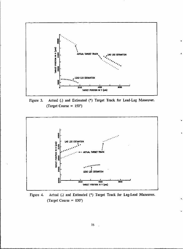
Figures 2 to 5 show actual and estimated Target positions- for four encounter

geometries with no error in bearing. So the only errors introduced are due to the linear

extrapolation of bearings. It is clear that lag-leg estimation is much more accurate than

the lead-leg-estimation. It is also clear that any attempt to regress estimated Target

positions over both legs can result in large errors.

L .EAD LEG ESflMATIDN

Xz

LAG LEG ESTIMAloN

4012000TARGEr POSITON IN Y (WO)

Figure 2. Actual ()and Estimated ()Target Track for Lead-Lag Maneuver.

(Target Course 0 60')' 0(,e

ACTUAL TARGET TRAK LAO LED EFTWATION

LEAD LEG ESTIMATION

02000 4SCOOKTA'ROET POSITION IN Y (rd.)

Figure 3. Actual ()and Estimated ()Target Track -for Lead-Lag Maneuver.

(Target Course = 150')

LAC LEO ESTIMATION

ACTUA TDTTRC

LEDLG ESITO

Figure 4. Actual ()and Estimated (*) Target Track for Lag-Lead Maneuver.

(Target Course =0300)

16

LAG LEG E1T A.TION/ LEAD LEG IMIMATION; . . ,o ,

A*.LWu TARGC TWXK

_4C .'0 5000 12000

INcRE1 POSMON IN Y COO)

Figure 5. Actual (.) and Estinw-ted (*) Target Track for Lag-Lead Maneuver.

(Target Course = 1201)

2. Explanation of Why Lag-Leg Estimation is Better than Lead-Leg Estimation

To help explain why the lag-leg estimation was better than lead-leg estimation,

scatter plots of bearings versus time for numerous encounter geometries were obtained.

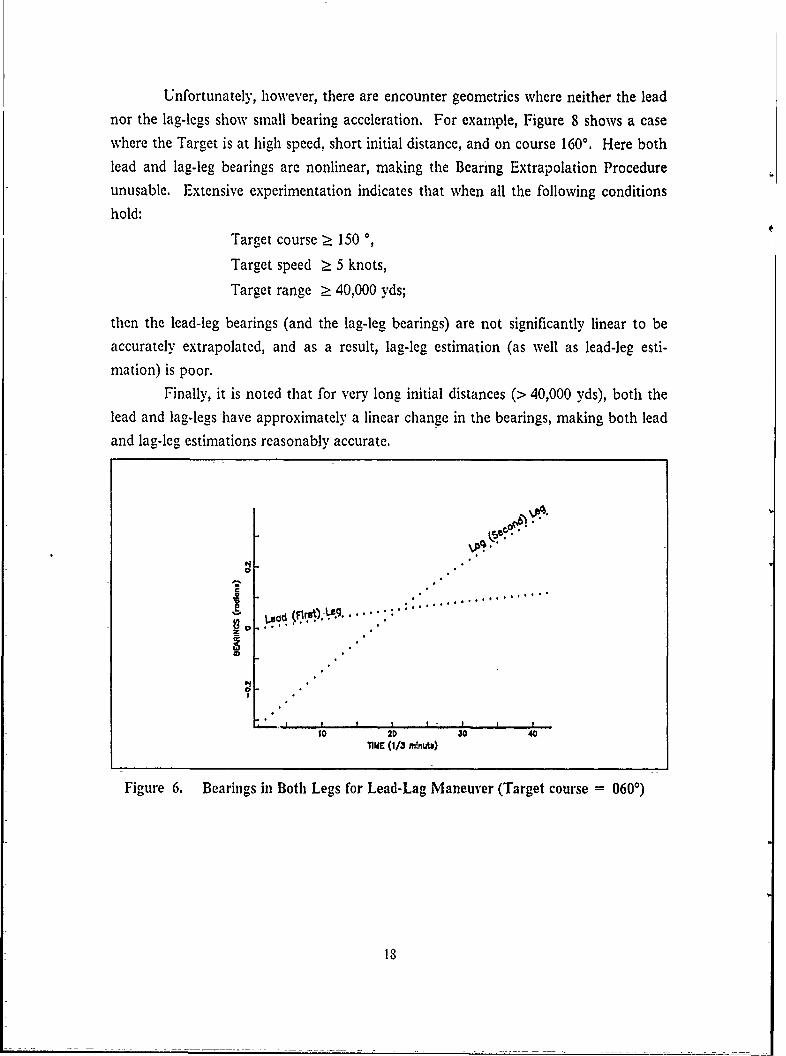
Figures 6, 7, and 8 are-typical. In Figure 6, a lead-lag encounter is represented. It was

observed that during the lead-leg (first leg), the bearing rate was generally smaller than

that of the lag-leg (second leg). Also, and perhaps more importantly, the change in

-bearing rate (bearing acceleration) was also -smaller in the lead-leg. When this happens,

it is possible to use linear regression to extrapolate the lead-leg bearings accurately into

the-future. This makes -the lag-leg estimation -more accurate. It is -clear from Figure 6

that if linear iegression were used to extrapolate the lag-leg bearings into the past, sig-

nificant errors would result, and these errors would likely cause-the lead-leg estimation

to be less accurate.

In the same fashion, Figure 7 shows a plot of bearings versus time for a typical

lag-lead cncountcr. Here also, the leadleg (second leg) has a smaller bearing rate and

bearing acceleration. So linear regression can be used to extrapolate accurately the

lead-leg bearings backward in time, again making the lag-leg estimation most accurate.

17

Unfortunately, however, there are encounter geometries where neither the leadnor the lag-legs show small bearing acceleration. For example, Figure 8 shows a casewhere the Target is at high speed, short initial distance, and on course 1600. Here both

lead and lag-leg bearings are nonlinear, making the Bearing Extrapolation Procedureunusable. Extensive experimentation indicates that when all the following conditions

hold:

Target course > 150

Target speed > 5 knots,

Target range > 40,000 yds;

then the lead-leg bearings (and the lag-leg bearings) are not significantly linear to beaccurately extrapolated, and as a result, lag-leg estimation (as well as lead-leg esti-

mation) is poor.

Finally, it is noted that for very long initial distances (> 40,000 yds), both the

lead and lag-legs -have approximately a linear change in the bearings, making both leadand lag-leg estimations reasonably accurate.

0

C ... .. .. .. .. . ..

u~ 9..... ..

s."

,,I,,, I - I f

10 20 30 40TIME (113 n,!nutv)

Figure 6. Bearings in Both Legs for Lead-Lag Maneuver (Target course = 0600)

18

Ie.c..... *

VA.Oll.

II I I I I10 20 30 40

TIME (I/3 minute)

Figure 7. Bearings in Both Legs for Lag-Lead Maneuver (Target Course = 1400)

44

- Lead (First) Leg."'

E. ............

z

! I I I I I I

10 20 30 -,OIME (1/ minute)

Figure 8. Bearings in Both Legs for Lead-lag Maneuver at Short Distance and

Closing Target.

19

F. CONCLUSIONS

1. Even when bearings were without error, the Bearing Extrapolation Procedure wasunsuccessful in estimating Target course and speed. However, range estimates werereasonable.

2. When bearing errors were introduced, range estimates also became inaccurate.3. For most encounter geometries, lag-leg estimation gave more -accurate results than

did lead-leg estimation. However, for some important cases both lag and lead-legestimations performed poorly.

20

III. POSSIBLE IMPROVEMENTS, AND ANALYSIS OF THEIR

ACCURACIES

The lack of accuracy of the proposed procedure, even under ideal conditions, led to

attempts to improve its performance. The following are some suggested minor changes

and two suggested major changes that were found to improve the accuracy of the Bear-

ing Extrapolation Procedure.

A. MINOR CHANGES

1. Increase in Leg Length

In an attempt to improve performance, several different leg lengths were tried.

It was discovered that leg lengths of 8 to 12 minutes gave the-best results. Shorter legs

gave too little data and longer legs resulted in nonlinear changes in lead-leg bearings.

Based on these tests, ten minutes was selected as the leg length for subsequent simu-

lation experiments.

2. Use of a Quadratic Model to Fair the Lag-Leg

Another important change from the original simulation that was tried was to

use a quadratic model to fair the bearings in the lag-leg. This produced better accuracy

in the estimated Target track parameters. It is noted that current-manual TMA methods

(in particular, the Time-Bearing Plot) use linear fairing.

3. Increase in Turn Time

Contrary to Ekelund ranging, if an instantaneous turn-is considered, large errors

in the estimated Target track parameters are generated. This is-because some actual and

corresponding extrapolated bearings are too close to each other-(i. e., a small baseline).

The intersection of those bearings often results in a estimated Target position far away

from the true position of the Target.

Based on these considerations, it was determined that the time-required for Own

Ship to turn should be increased. After many trials, it was found-that the best turn du-

ration is ten minutes, if leg length is also ten minutes. For longer times, the bearing rate

in the lead-leg does not remain low and constant, reducing the accuracy of the lkad-leg

bearing extrapolation,

21

B. ELIMINATION OF THE LEAD-LEG-ESTIMATION

As shown in Chapter II, when linear extrapolation of the bearings from the lag-leg

is used, increased errors are generated in the estimation of the Target track parameters.

This occurs because- the lag-leg generates a high and variable bearing rate compared to

the lead-leg. A simple solution to the problem is to drop the estimated Target positions

generated by the extrapolation of the lag-leg bearings.

One problem with this idea is that a lead-lag maneuver will then produce more ac-

curate estimates of Target position at the end of the maneuver than will a lag-lead ma-

neuver. This occurs since in the lead-lag case, the estimated Target positions are

obtained for times during the second (i.e., the lag) leg. And in the lag-lead case, the es-

timated Target positions are for times in the first (again, the lag) leg. So tW use a lag-lead

maneuver to estimate Target positions at the end of the maneuver requires that these

positions be extrapolated in time using derived estimates of Target course and speed.

This leads to accumulated errors in the final Target position.

To test for the possible improvements that might result when using only lag-leg es-

timation, simulation experiments were-conducted with-the -following parameters:

1. Speed of Own Ship: 5, 10, and 15 knots.

2. Speed of the Target: 5, 15, and 25 knots.

3. Initia! range: large (= 60,000), medium (= 30,000), and short ( 10,000) yds.

4, Only the lead-lag maneuver is considered.

5. Only the initial lead angle of 90 is cosidered.

6. Leg length: 4 minutes.

7. Time between legs: 6 minutes.

S. Standard deviation bearing error: 00, 0.50, 1.00, and 1.50.

9. Bearings for the first leg were faired and extrapolated linearly.

10. Bearings in- the- second leg were faired linearly.

It is important to note that other values for lead angle were not considered because,

as discussed in Chapter II, it was found that the best results were obtained-for a 90' lead'

angle.

In order to show -how the minor changes improve the performance of this major

suggested change (i. e., elimination of the lead-leg estimation), the simulation was run

for three different cases:

22

1. Without Minor Changes

The simulation program was run 100 times for each combination of the above

parameter values. It was determined that for the ideal case (O° bearing errors) the ac-

curacy of the predicted Target parameters was adequate, but with bearing errors intro-

duced, large errors in all three Target parameters were produced. So it was concluded

that simply eliminating the lead-leg estimation was not a sufficient improvement.

2. With Increased Leg Length and Lag-Leg Faired with a Quadratic Model

Here leg length was increased to ten minutes and the lag-leg was faired with a

quadratic model. The same simulation experiments were run as before. Only the results

for lead-lag maneuvers are presented in Table 5. Lag-lead maneuvers gave uniformly

worse results for reasons discussed above. Additionally, and more surprisingly, the ac-

curacy for the lag-lead maneuver was not as good as the lead-lag, even when estimating

the Target parameters at the end of the first leg. This was a confirmation that, in gen-

eral, the lead-lag maneuver gives better results than do lag-lead [Ref. 7: pp. 3].

Results for estimated Target course and speed were- very precise only when the

bearing error was zero and when Own Ship speed was greater than- ten knots. When

errors in bearings were included, the accuracy in estimated Target course and'speed was

tremendously reduced. For example, for large initial- distance and 15 knots Own Ship

speed the following was obtained:

1. With no bearing error, the error in estimated speed was always less than 10% andthe error in course was less than 100 in 83% of the different geometries.

2. With a small bearing error (standard deviation = 0.5"),-only 33.4% of the runs hadan error in speed of less than 10% . In 15.1% of the runs, the error in course wasless than 100.

One of the conclusions of this study is that the Bearing Extrapolation Procedure, even

as modified here, does not produce accurate estimates of Target-course- and speed. With

Target range, however, more success was obtained. Table 5 shows the percentage of

simulation runs that produced an estimated Target range at the end of the maneuver

within 5%o, 10/o, and 20% of the true range.

23

Table 5. ACCURACY IN ESTIMATED RANGE WHEN ONLYLAG-LEG-ESTIMATION IS USED. (LEG LENGTH = 10 MIN).

n Si Percentage of times the absolute error isOwn Ship St. Dev. Initial dis- smaller than 5%, 10%, and 20% of ac-

speed bearing er- tance tual for range.(knts) ror 5% 10% 20%

large 21.6 41.7 72.1


1.00 medium 35.4 62.9 86.6

short 10.7 18.6 40.215 .... __ __

large 49.9 78.8 93.70.50 medium 43.8 71.1 88.6

short 10.3 18.9 39.6

large 72.2 88.9 94.40.00 medium 55.6 77.8 88.9

short 11.1 22.2 38.9large 15.2 30.6 55.9

1.50 medium 20.2 39.4 70.7

short 16.4 32.4 51.3large 21.0 41.2 70.1

1.00 medium 26.2 .9.5 76.610 short 16.1 32.7 52.6

large 35.4 62.1 88.7

0.50 medium 35.4 61.3 79.5

short 15.3 32.3 52.5

largc 72.2 77.8 94.4

0.00 medium 38.9 72.2 77.8short 16.7 27.8 50.0

From Table 5 it can be seen that the larger the Own Ship speed the better is

the estimate of range. This is shown in Figure 9 which is the plot of the accuracy in

estimated ran2e versus standard deviation of bearing errors when the Own Ship speed

24

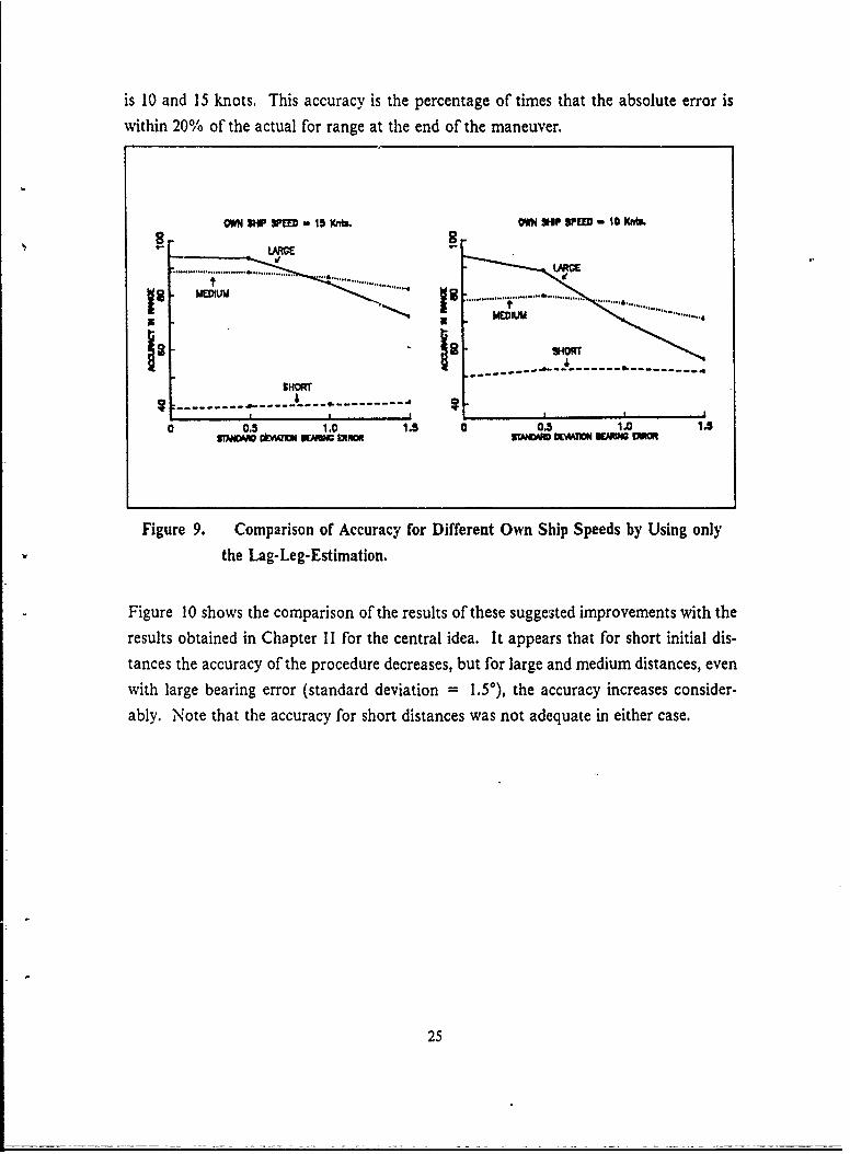
is 10 and 15 knots. This accuracy is the percentage of times that the absolute error iswithin 20% of the actual for range at the end of the maneuver.

MN SH WPlD - 15 Kn& 0W SIP SPEW - 10 Kff.8"I,

.... ..... .... . ..... ....".

M M .. . . .. . . .. . . .. . . . .... ...... ............... ....... ....

------------------------- --- k-----------------SHORT

0 0!5 1!0 1 .5 0..5 1.0 1.3

KNOMM ObW=C NEAMO 1XR SW OMBE=M

Figure 9. Comparison of Accuracy for Different Own Ship Speeds by Using only

the Lag-Leg-Estimation.

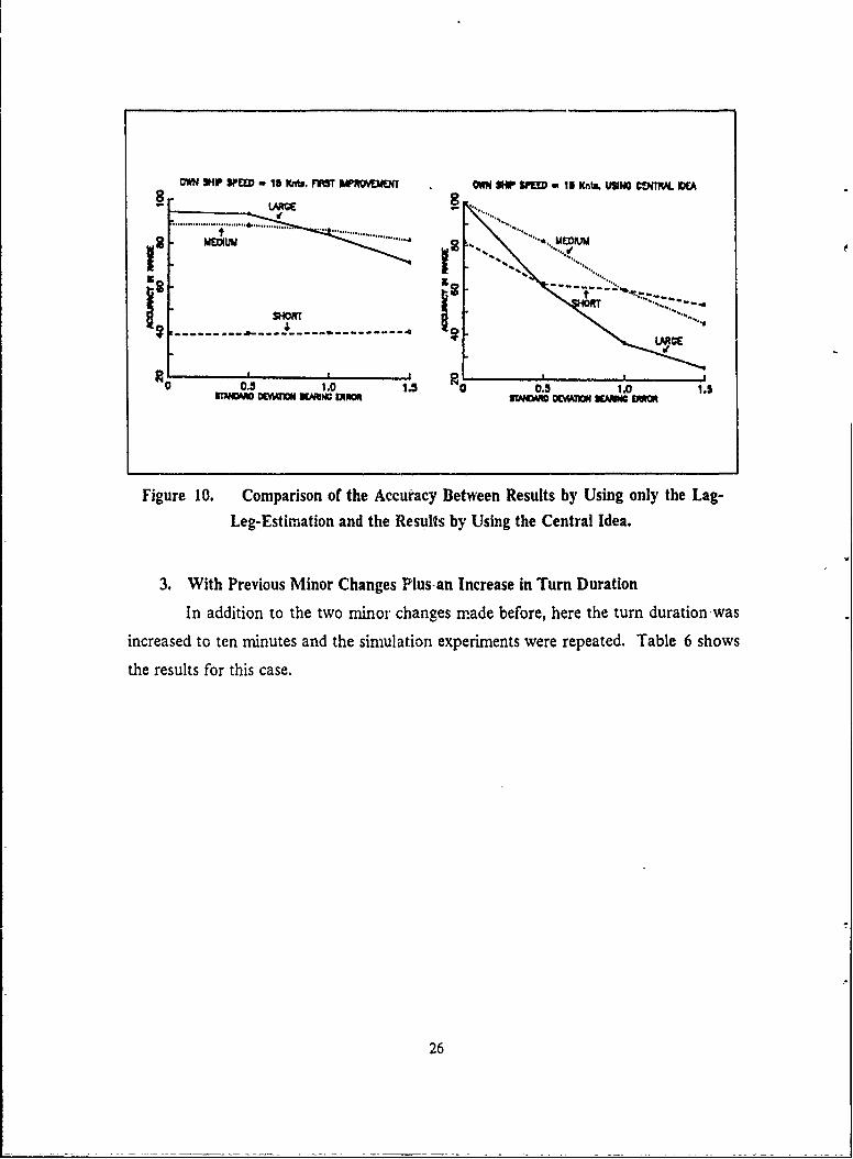
Figure 10 shows the comparison of the results of these suggested improvements with the

results obtained in Chapter II for the central idea. It appears that for short initial dis-tances the accuracy of the procedure decreases, but for large and medium distances, even

with large bearing error (standard deviation = 1.50), the accuracy increases consider-

ably. Note that the accuracy for short distances was not adequate in either case.

25

0"N SHP SFEW 15 Xnt. F1VT U'ROEMO( . OWN SW SPEW - 15 Xntik USNO C?4ThA VEA

LAG

... ..... ...

mmmMEDIUU

0. ! 13 9 0 0.9 1.0O 1.5STNW DYM KNW i W 3WO; OCWAflUUN WAM W

Figure 10. Comparison of the Accuracy Between Results by Using only the Lag-Leg-Estimation and the Results by Using the Central Idea.

3. With Previous Minor Changes Plus-an Increase in Turn Duration

In addition to the two midnor changes made before, here the turn durationwas

increased -to- ten minutes and the simulation experiments were repeated. Table 6 shows

the results for this case.

26

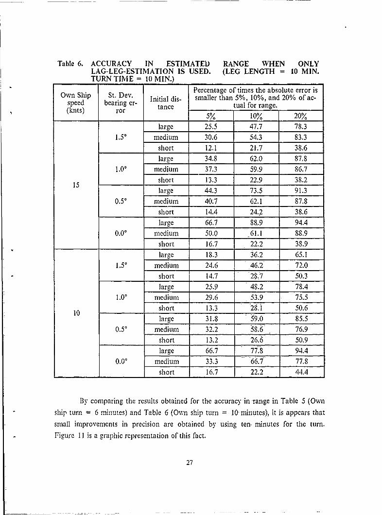
Table 6. ACCURACY IN ESTIMATED RANGE WHEN ONLYLAG-LEG-ESTIMATION IS USED. (LEG LENGTH = 10 MIN.TURN TIME = 10 MIN.)


speed bearing er- tance tual for range.(knts) ror 10% 20%

large 25.5 47.7 78.31.50 medium 30.6 54.3 83.3

short 12.1 21.7 38.6

large 34.8 62.0 87.81.0° medium 37.3 59.9 86.7

15 short 13.3 22.9 38.2

large 44.3 73.5 91.30.50 medium 40.7 62.1 87.8

short 14.4 24.2 38.6

large 66.7 88.9 94.40.00 medium 50.0 61.1 88.9

short 16.7 22.2 38.9large 18.3 36.2 65.1

1.50 medium 24.6 46.2 72.0

short 14.7 28.7 50.3large 25.9 48.2 78.4

1.0° medium 29.6 53.9 75.5

10 short 13.3 28.1 50.6large 31.8 59.0 85.5

0.50 medium 32.2 58.6 76.9

short 13.2 26.6 50.9

large 66.7 77.8 94.40.00 medium 33.3 66.7 77.8

I short 16.7 22.2 44.4

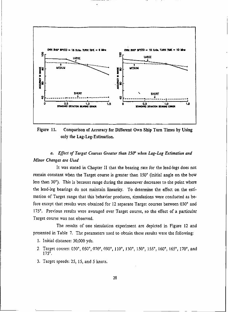
By comparing the results obtained for the accuracy in range in Table 5 (Own

ship turn = 6 minutes) and Table 6 (Own ship turn = 10=minutes), it is appcars that

small improvements in precision are obtained by using ten minutes for the turn.

Figure 11 is a graphic representation of this fact.

27

OWN SHP ,1 Kn W.IN Ttk OW N "P O SrEt D -, I I Kb.TUIN '.%A 10 Mkw

[ SHORr ' SHORT- -- - -- - ---------------- ----- -- 4- - - - - - -.- 9 --- 4

0.5 1.0 1.5 0 ' 0. 1.0 1.11

Figure 11. Comparison of Accuracy for Different Own Ship Turn Times by Using

only the Lag-Leg-Estimation.

a. Effect of Target Courses Greater than 150' when Lag-Leg Estimation and

Minor Changes are Used

It was stated in Chapter II that the bearing rate for the lead-legs does not

remain constant when the Target course is greater than 1500 (initial angle on the bow

less than 300). This is because range during the maneuver decreases to the point wherethe lead-leg bearings do not maintain linearity. To determine the effect on the esti-

mation of Target range that this behavior produces, simulations were conducted as be-fore except that results were obtained for 12 separate Target courses between 0300 and

1750. Previous results were averaged over Target course, so the effect of a particular

Target course was not observed.

The results of one simulation experiment are depicted in Figure 12 and

presented in Table 7. The parameters used to obtain these results were the following:

1. Initial distance: 30,000 yds.

2. Target couses: 030', 050, 070, 0900, 1100, J300 , 1500. 1550, 1600, 1650, 1700, and175".

3. Target speeds: 25, 15, and 5 knots.

28

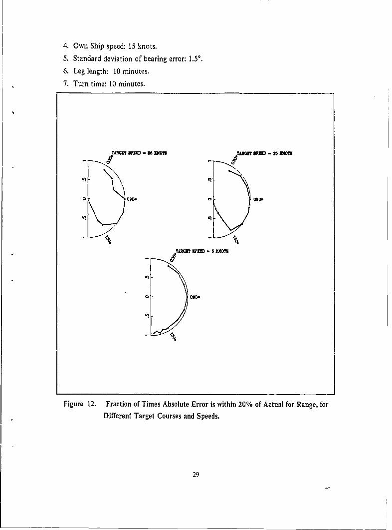
4. Own Ship speed: 15 knots.

5. Standard deviation of bearing error: 1.5°.

6. Leg length: 10 minutes.

7. Turn time: 10 minutes.

k IT WED - 2 In TAI UD - 15 D'II

0V 0 OO

Ui n

Figure 12. Fraction of Times Absolute Error is within 20% of Actual for Range, for

Different Target Courses and Speeds.

29

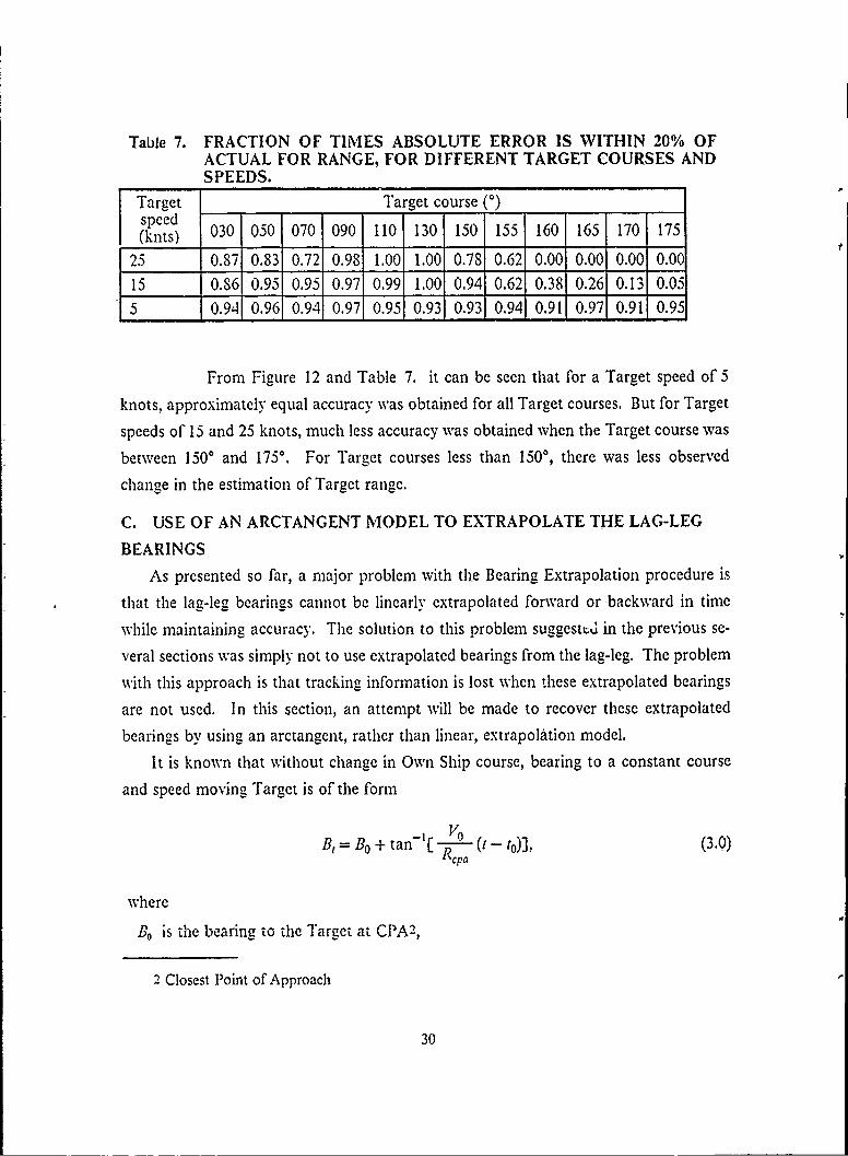
Table 7. FRACTION OF TIMES ABSOLUTE ERROR IS WITHIN 20% OFACTUAL FOR RANGE, FOR DIFFERENT TARGET COURSES ANDSPEEDS.

Target Target course (0)speed(knts) 030 050 070 090 110 130 150 155 160 165 170 175

25 0.87 0.83 0.72 0.98 1.00 1.00 0.78 0.62 0.00 0.00 0.00 0.00

15 0.86 0.95 0.95 0.97 0.99 1.00 0.94 0.62 0.38 0.26 0.13 0.05

5 0.94 0.96 0.94 0.97 0.95 0.93 0.93 0.94 0.91 0.97 0.91 0.95

From Figure 12 and Table 7. it can be seen that for a Target speed of 5

knots, approximately equal accuracy was obtained for all Target courses. But for Target

speeds of 15 and 25 knots, much less accuracy was obtained when the Target course was

between 1500 and 1750. For Target courses less than 150 °, there was less observed

change in the estimation of Target range.

C. USE OF AN ARCTANGENT MODEL TO EXTRAPOLATE THE LAG-LEG

BEARINGS

As presented so far, a major problem with the Bearing Extrapolation procedure is

that the lag-leg bearings cannot be linearly extrapolated forward- or -backward in time

while maintaining accuracy. The-solution to this problem suggesttd in the previous se-

veral sections was simply not to use extrapolated bearings from the lag-leg. The problem

with this approach is that tracking information is lost when these extrapolated bearings

are not used. In this section, an attempt will be made to recover these extrapolated

-bearings by using an arctangent, rather than linear,- extrapolation model.

It is known that without change in Own Ship-course, bearing to a constant course

and speed moving Target is of the form

Bt = B0 + tan- h--- (t - to)], (3.0)lcpa

where

B0 is the bearing to the Target at IP A2,

2 Closest Poit of Approach

30

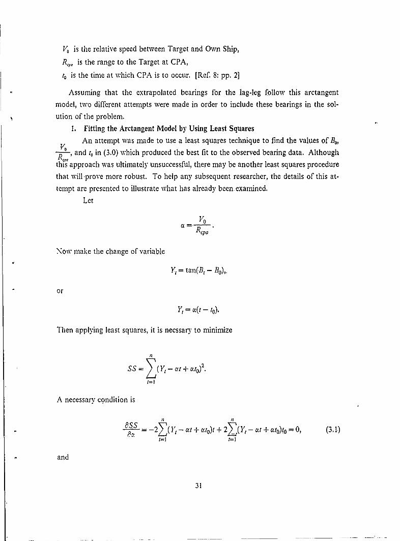
V/0 is the relative speed between Target and Own Ship,

R.Po is the range to the Target at CPA,

t. is the time at which CPA is to occur. [Ref. 8: pp. 2]

Assuming that the extrapolated bearings for the lag-leg follow this arctangent

model, two different attempts were made in order to include these bearings in the sol-

ution of the problem.

1. Fitting the Arctangent Model by Using Least Squares

An attempt was made to use a least squares technique to find the values of B,

R and t, in (3.0) which produced the best fit to the observed bearing data. Although

ths approach was ultimately unsuccessful, there may be another least squares procedure

that will -prove more robust. To help any subsequent researcher, the details of this at-

tempt are presented to illustrate what has already been-examined.

Let

Vo

Repa

Now make the change of variable

Yz tan(B, - Bo) ,

or

= a(t - to).

Then applying least squares, it is necssary to minimize

SS= (Yt - cat +ss 1o) 2 .

t=l

A necessary condition is

n ?I

-2..( t- at + ato)t + 27_()'t - at +ato)to = 0, (3.1)

and

31

-t

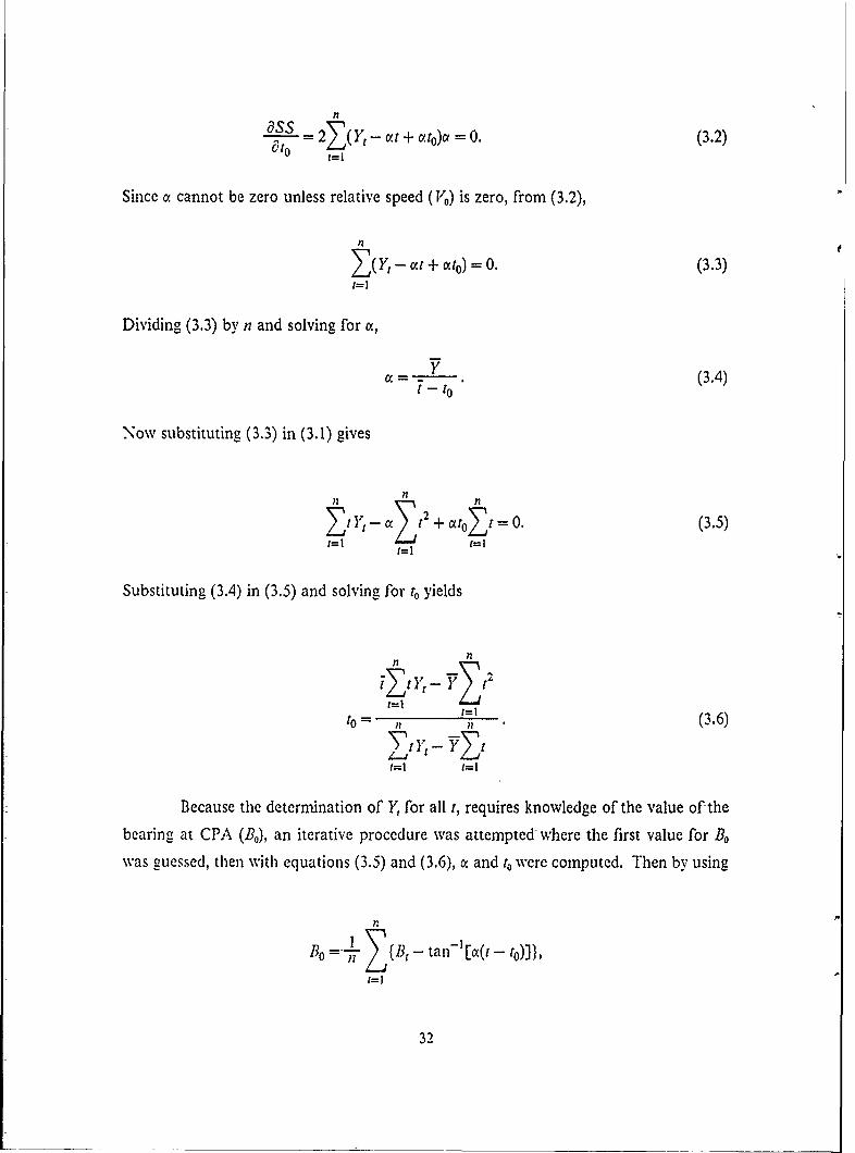
OSS 2 2 (Yt - t + .to)o = O. (3.2)10 1=1

Since . cannot be zero unless relative speed (I') is zero, from (3.2),

nY( Yt - at + Oto) 0 . (3.3)

Dividing (3.3) by n and solving for c,

- _(3.4)

Now substituting (3.3) in (3.1) gives

n

71- Y 0 t 2 + to t= 0. (3.5)

Substituting (3.4) in (3.5) and solving for to yields

~nI-t F t 2

t=1 t=l

to = (3.6)Zt~t- Y~t

Because the determination of I, for all t, requires knowledge of the value of-the

bearing at CPA (B,), an iterative procedure was attempted where the first value for B.

was guessed, then with equations (3.5) and (3.6), o. and to were computed. Then by using

Bo B, 1- tan-I[.(t-

32

a new value for Bo was obtained. This iteration was continued in an attempt to converge

on the true B. Unfortunately for even small errors in bearings, (standard deviation =

0.5*). the procedure would not reliably converge.

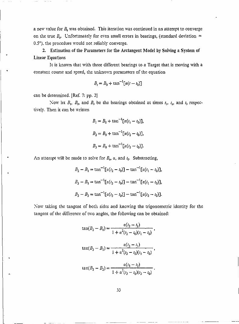
2. Estimation of the Parameters for the Arctangent Model by Solving a System of

Linear Equations

It is known that with three different bearings to a Target that is moving with a

constant course and speed, the unknown parameters of the equation

Bt = Bo + tan-'1.(t - to)]

can be determined. [Ref. 7: pp. 2]

Now let B,, B2, and B3 be the bearings obtained at times tj, t., and 13 respec-

tively. Then it can be written

B, = B0 + tan-'[.(tj - to)],

B2 = Bo + tan-'[.(t2 - to)],

B3 = Bo + tan-'[o(t 3 - to)].

An attempt will be made to solve for B,, a, and to. Substracting,

B2- Bi = tan-'[(t 2 - to)] - tan-l[(t - to)],

B3 - B1 = tan-'[a(t3 - to)] - tan-' [.(t1 - to)],

B3 - B2 = tan-1[c.(t 3 - to)] - tan- [1C (t 2 - t0)].

Now taking the tangent of both sides and knowing the trigonometric identity for the

tangent of the difference of two angles, the following can be obtained:

tan(132 - B,) = 2 - -

1 + . (13 - to)(t to)

- 12)

tan(B3 - B2 ) =i+ a :.(13 - 10)(12 - 0

33

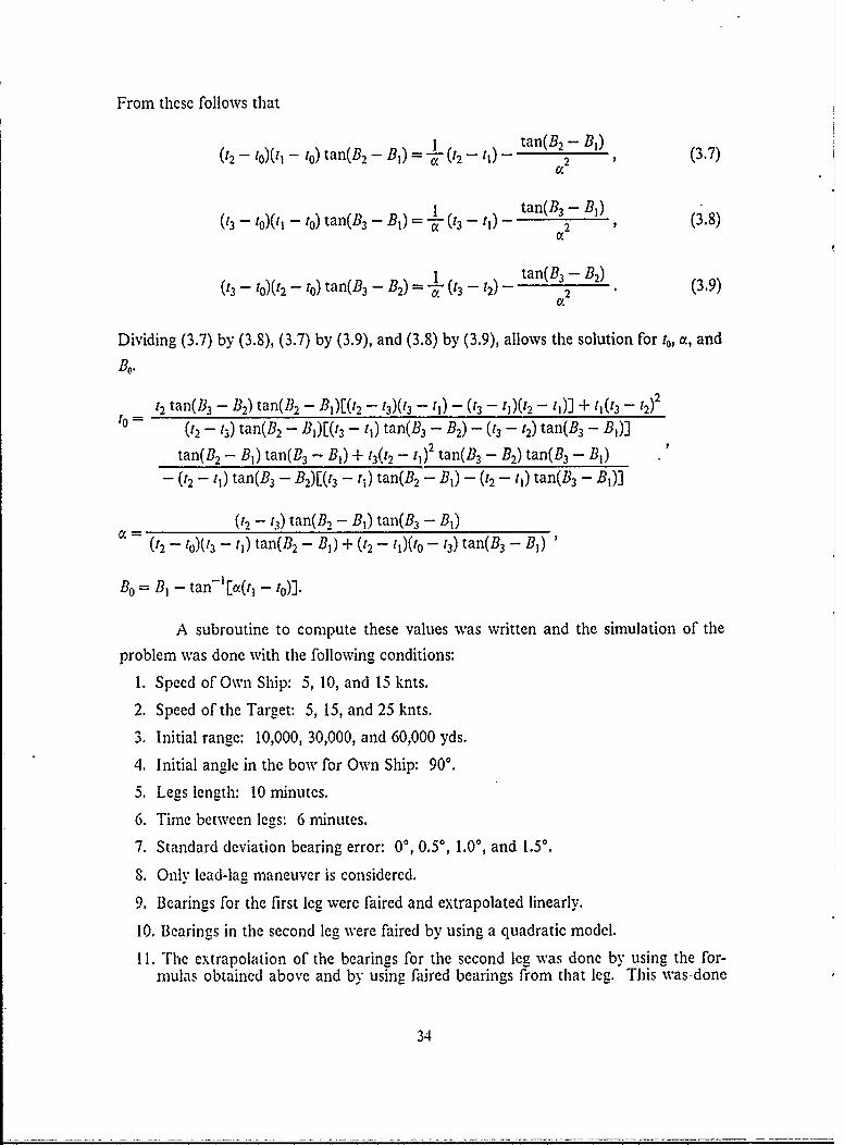
From these follows that

= - -tan(B 2 -B0)('2 - 4o)(fi - to) tan(B2 - BI) = 1 (t2 - t) (3.7)

1 tan(B3 - BI)(t3 - to)(t, - to) tan(B3 - BI) = (t3 - -) - (3.8)-

= 1 - ~) -tan(B 3 - B 2 )_(t3 - tO)(2 - 1o) tan(B3 - B2) =' oi (3 2 2 (3.9)

Dividing (3.7) by (3.8), (3.7) by (3.9), and (3.8) by (3.9), allows the solution for to, (X, and

B0.

r 2 tan(B3 - B2) tan(B2 - B 1)[(t2 - t3)(3 - ti) - (3 - tl)(t2 - r,)] + 1t(3 - t2)2

to (t2 - 13) tan(B2 - B,)[( 3 - tj) tan(B3 - B2) - (t3 - t2) tan(B3 - B,)]

tan(B2 - BI) tan(B3 - BI) + 13(2 - t,)2 tan(B3 - B2) tan(B3 - BI)

-(t 2 - t,) tan(B3 - B2)[(r3 - tj) tan(B2 - BI) - (t2 - t,) tan(B3 - B,)]

('2 - 13) tan(B, - BI) tan(B3 - BI)

(2- 1())(i3 - 4rj) tan(B2 - B0) + (t2 - ION(' - 13) tan(B3 - BI)

B0 = B, - tan-' [.(t - to)].

A subroutine to compute these values was written and the simulation of the

problem was done with the following conditions:

1. Speed of Own Ship: 5, 10, and 15 knts.

2. Speed of the Target: 5, 15, and 25 knts.

3Initial range: 10,000, 30,000, and 60,000 yds.

4. Initial angle in the bow for Own Ship: 900.

5. Leg~s length: 10 minutes.

6. Time between legs: 6 minutes.

7. Standard deviation bearing error: 0', 0.50, 1.0%, and 1.50.

8. Only lead-lag maneuver is considered.

9. Bearings for the first leg were faired and extrapolated linearly.

10. Bearings in the second leg were faired by using a quadratic model.

11. The extrapolation of the bearings for the second leg was done- by using the for-mnulas obtained above and by using faired bearings from that leg. This was-done

34

because the use of raw bearings produced too much error in the estimation of theparameters of the Target.

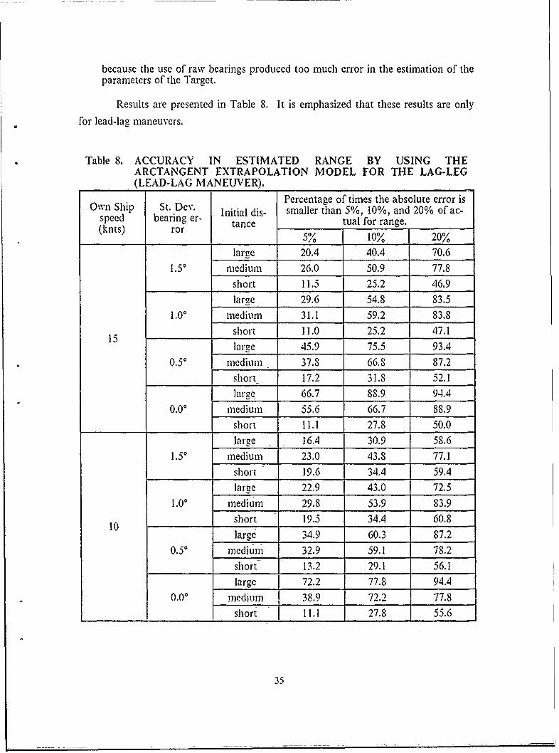
Results are presented in Table S. It is emphasized that these results are only

for lead-lag maneuvers.

Table 8. ACCURACY IN ESTIMATED RANGE BY USING THEARCTANGENT EXTRAPOLATION MODEL FOR THE LAG-LEG(LEAD-LAG MANEUVER).


speed bearing er- tance tual for range.(knts) ror 5% 10% 20%

large 20.4 40.4 70.61.50 medium 26.0 50.9 77.8

short 11.5 25.2 46.9large 29.6 54.8 83.5

1.00 medium 31.1 59.2 83.8

15 short 11.0 25.2 47.1lar-ee 45.9 75.5 93.4

0.50 medium 37.8 66.S 87.2short- 17.2 31.8 52. 1

large 66.7 88.9 94.40.00 medium 55.6 66.7 88.9

short 1-1.1 27.8 50.0large 16.4 30.9 58.6


1.00 medium 29.8 53.9 83.9

10 short 19.5 34.4 60.8large 3 4.9 60.3 87.2

0.50 medium 32.9 59.1 78.2

short 13.2 29.1 56.1large 72.2 77.8 94.4

0.00 medium 38.9 72.2 77.8short I1.1 27.8 55.6

35

Comparing these results with those on Table 3 on page 13, it is clear that this

procedure performs better than the original (unimproved) Bearing Extrapolation Proce-

dure. However, the results are about the same as those in Table 8, indicating that sim-

ply not using the lag-leg extrapolated bearings is just about as effective as trying to

extrapolate them with the arctangent model.

36

IV. CONCLUSIONS AND RECOMMENDATIONS

1. CONCLUSIONS

1. The proposed procedure does not allow estimation, with adequate accuracy, of theTarget track parameters when linear bearing extrapolation is used for both legs(central idea). Linear bearing extrapolation is only valid for lead-legs where lowand constant bearing rate is obtained. For lag-legs the bearing rate is generallyhigher and more variable.

2. Adequate accuracy for course and speed is not obtained using any of the examinedprocedures unless bearing error is zero (ideal conditions).

3. Adequate accuracy in estimated range for large and medium initial distances canbe obtained if.

a. Quadratic faired bearings from the lag-leg are used in combination with linearextrapolated bearings from the lead leg.

b. Lead-lag maneuver is performed.

c. Lead angle close to 900 is used.

d. Leg length is larger than seven minutes and less than twelve minutes.

e. Own ship turn time is larger than six minutes and less than ten minutes.

f. Angle on the bow is not smaller than 300. If it is, then Target speed is notgreater than 5 knots.

4. Adequate accuracy in range for short initial distances is obtained only when theTarget is not closing the Own Ship.

2. RECOMMENDATIONS

1. If this procedure is implemented. use only extrapolated bearings from the lead leg(low and constant bearing rate) and faired bearings for the lag-leg (high and vari-able bearing rate).

2. Further research should be done to obtain a model that allows use of the extrapo-lated bearings obtained from the lag-leg.

37

APPENDIX A. DISCUSSION OF SELECTED SOLUTION METHODS

A. SPIESS RANGING

Spiess theory establishes that the problem of obtaining satisfactory solutions for a

bearings-only approach against targets moving with a constant course and speed, can

be solved by using four bearings and at least one change of course or speed by Own

Ship. With this in mind, several graphical methods capable of giving quick reliable sol-

utions were developed. [Ref. 3]

From the Passive Ranging Manual, Volume III, the basic graphical method for

Spiess ranging is explained as follows:

Given three bearings to the Target, observed at times t, r2 , and t3 togetherwith a fourth time, t,, the locus, L, of all possible Target position! at time, t,, for allpossible Target tracks which satisfy the three bearings at t,, t2, and t3, and whichmaintain a constant course and speed. is a straight line. The actual position of theTarget at time, r,, is determined by the intersection of L with the observed bearingat time, t,, (provided SSK changes course and speed).

This locus, L, can be determined by picking out two arbitrary Target trackswhich satisfy the three-bearing conditions, and plotting the position of the Targeton these tracks at time 1, Then L is the line through these two plotted positions.This is the basis of the Spiess four-bearing TMA. The bearing lines at t,, t2, and t3are used to find the locus of Target positions at t4. The intersection of this locuswith the bearing line at t, determines one -point on the track. Another point is de-teramined by using the bearing lines at t2, t3 , and t4 to find the locus of Target posi-tions at zt. The intersection of this locus with the bearing line at t, determinesanother point on the track. The track is then the line joining the two constructedTarget positions.

Because bearings are not precise enough to- apply this method, faired bearings are

usually used.

B. EKELUND RANGING

The basic Ekelund solution for a constant course and speed moving Target is based

on a two leg maneuver by Own Ship. During these legs, Own Ship records actual Target

bearings. The rate of change of the bearings-is computed for each leg by applying linear

least squares techniques. This method assumes that during the turn the distance that

Own Ship moves and the change of angle in the bow can be disregarded; i.e., assumes

an instantaneous turn. Given this assumption, the range to the Target can be computed.

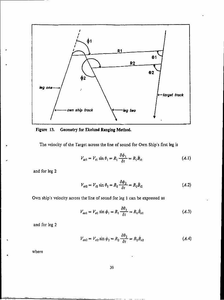
Using Figure 13, derivation of range is as follows:

38

8R

log one

target track

4---own ship track kgtwo

Figure 13. Geometry for Ekelund Ranging Method.

The velocity of the Target- across -the line of sound for Own Ship's first leg is

V.,11 = VIl sin 01 -- R, RI[

and for leg 2

Va VSin 2 = R2 a 2 Rh (A.2)at

Own ship's velocity across the line of sound for leg I can be expressed as

Vaoi = Vol sin R, = =R]t(A.3)

and for leg 2

V 2 = V02 sin c, R, a0 2 = R2Bo2 (A.4)

where

39

= Bearing rate of Target in leg i.

R, = Range to the Target at the turn.

R2 = Range to the Target after the turn.

ll, = Velocity of Own Ship in leg i.

, = Velocity of the Target in leg i.

Assuming Target velocity remains constant during Own Ship maneuvering; i.e.,

Va = V,2 = V, and that the angle in the bow also remains approximately constant; i.e.,

01 02 = 0, and that the range to the Target does not appreciably changes; i.e.,

R= R2 = R,, then equations (A.1), (A.2), (A.3), and (A.4) can be written as

V, sin 01 = Rebtl, (A.5)

T, sin 0 = ReBha , (A.6)

Vol sin 0 = ReBol, (A.7)

1"o2 sin 4i = RABo 2. (A.8)

and by subtracting (A.7) from (A.5) and (A.8) from (A.6)

V, sin 0 - Vl sin 01 = Re(Bh - Boi) = ReI3i,

V sin 0 - V02 sin b2 = Re(b. 2 - Bo2) = ReB 2"

Subtracting these last two equations yields

1/0, sinO I - "o2 sin0 2R- B2 i '

where, B, = bearing rate of Target relative to Own Ship in leg i.

The problems in accuracy with this method are:

I. It assumes that Own Ship can perform the two legs maneuver with an instantane-ous turn-[Ref. 9: pp. 1-3].

2. The Ekelund Range Equation is dependent on the ratio of the bearing -rates -devel-oped on the two legs of the ranging maneuver which are small and not very precisevalues [Ref. 9: pp. 1-3.

40

3. In practice, measuring the bearing rate involves a bearing smoothing process whichtakes place over a portion of each leg and results in bearing rates at times signif-icantly different from the time of the turn [Ref 9: pp. 3-2].

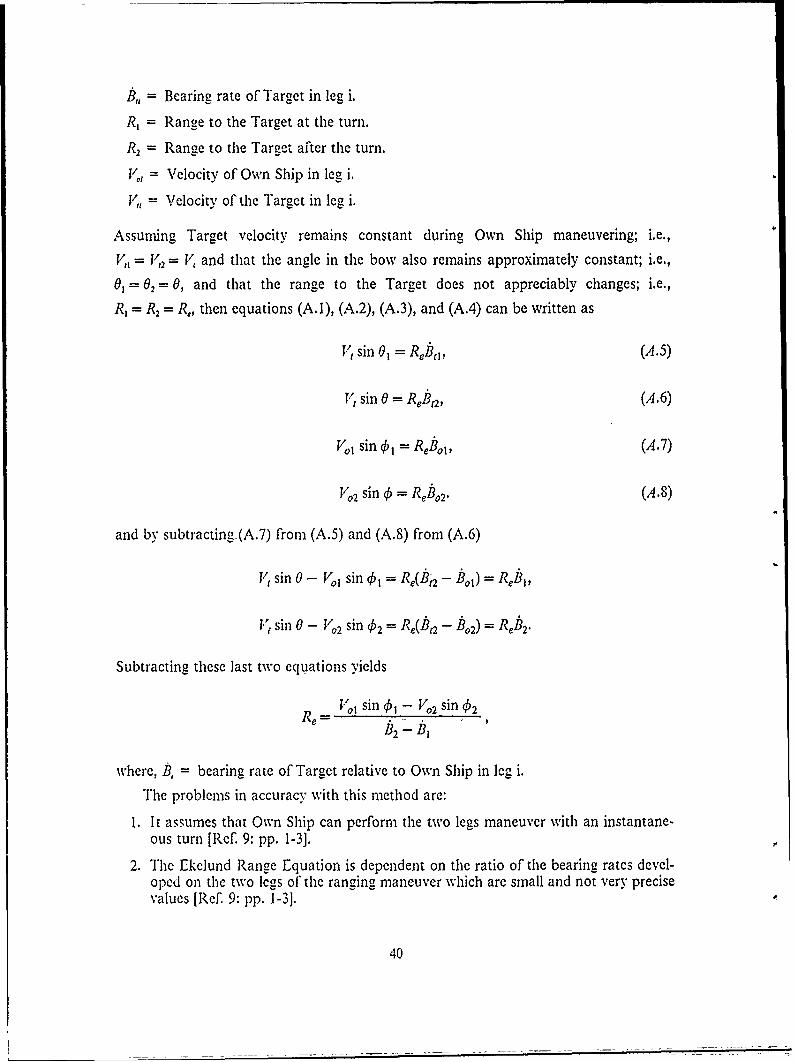
C. CHURN METHODThe basic concept of CHURN TMA is similar to that of the strip plot and includes

in its solution the Spiess TMA for the particular case where there are only four bearinglines computed [Ref. 9: pp. 7-1, 7-31. Figure 14, depicts the regular CHURN TMA

method.

estimatedt2 target track

N Bi = bearing

J1 82 83 94 195 196 87 8I

13 4 own ship track

Figure 14. Geometry for CHURN Method.

Own Ship performs a two leg maneuver during which it measures bearings to aTarget that is moving with constant course and speed. The CHURN method takes those

bearings and fits a Target track to them using the perpendicular distance between a given

bearing line and the corresponding Target position on the fitted track as a measure ofthe goodness of fit. Applying the concept of least squares, the best Target track is that

which then minimizes the sum of squares of these distances.[Ref. 9: pp. 7-2 ]

41

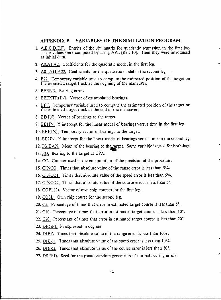
APPENDIX B. VARIABLES OF THE SIMULATION PROGRAM

1. A.B.C.D.E.F. Entries of the A-' matrix for quadratic regression in the first leg.These values were computed by using APL [Ref. 10]. Then they were introducedas initial data.

2. AO.AI.A2. Coefficients for the quadratic model in the first leg.

3. A01.A1 1.A22. Coefficients for the quadratic model in the second leg.

4. B22. Temporary variable used to compute the estimated position of the target onthe estimated target track at the begining of the maneuver.

5. BEERR. Bearing error.

6. BEEXTR(IN). Vector of extrapolated bearings.

7. BFF. Temporary variable used to compute the estimated position of the target onthe estimated target track at the end of the maneuver.

8. BE(IN). Vector of bearings to-the target.

9. BE1IN. Y intercept for the linear model of bearings versus time in the first leg.

10. BEI(IN). Temporary vector of bearings to the target.

11. BE21N. Y intercept for the-linear model of bearings versus time in the second leg.

12. BMEAN. Mean of the bearing to the target. Same variable is used for-both-legs.

13. BO. Bearing to the target at CPA.

14. CC. Counter used in the-computation of the precision of the procedure.

15. CINCO. Times that absolute-value of the range error is less than 5%.

16. CINCO1. Times that absolute value of the speed error is less than 5%.

17. CINCO2. Times that absolute value of the course error is less than 5*.

18. COFL(2). Vector of own ship-courses for the first leg..

19. COSL. Own ship course-for the second leg.

20. C5. Percentage of times-that error in estimated target course is less than 5*.

21. CIO. Percentage of times that error in estimated target course is less than 100.

22. C20. Percentage of times that -error in estimated target course is less than 20*.

23. DEGPI. Pi expressed-in degrees.

24. DIEZ. Times that absolute value of the range error is less than 10%.

25. DIEZI. '1 imes that absolute value of the speed error is less than 10%.

26. DIEZ2. Times that absolute value of the course error is less than 100.

27. DSEED. Seed for the pseudorandom generation of normal bearing errors.

42

28. ECTLR. Estimated target course obtained by linear regression on the target fixes.

29. ERANTL. Estimated range to the target at the end of the maneuver.

30. ESLOPE. Temporary variable corresponding to the target course.

31. ESPTL. Estimated speed of the target.

32. EXT(IN). Vector of estimated target positions in the X axis.

33. EYINT. Y intercept of the estimated target course.

34. EYT(IN). Vector of estimated target positions in the Y axis.

35. FBE(IN). Vector of faired target bearings.

36. IN. Time to complete the maneuver in 1/3 of minutes.

37. INFO(IN). Flag used to signal when Estimated X position of the target is equalto the X position of the own ship.

38. IX(3). Vector of initial target distances from own ship in the X axis.

39. IY(3). Vector of initial target distances from own ship in the Y axis.

40. LLL. Counter to determine the amount of fixes used in the regression to determinetarget track.

41. PER. Percentage error in range computed from the estimated and the simulatedrange to the target at the end of the maneuver.

42. PERI. Percentage error in speed computed from the estimated and the simulatedtarget speed.

43. PER2. Amount of error in course computed from the estimated and the simulatedtarget course.

44. Pl. Pi in radians.

45. R.S.T.U.V.W. Entries of the A-' matrix for quadratic regression in the second leg.These values were computed by using APL [Ref. 10]. Then they introduced as ini-tial data.

46. RANGEF. Simulated range to the target at the end of the maneuver.

47. RCBFL 1. Rate of change of bearing during the first leg. This value is computedassuming che linear model for the bearings versus time.

48. RCBSLI. Rate of change of bearing during the Second leg. This value is computedassuning the linear model for the bearings versus time.

49. R5. Percentage of times that error in estimated range to the target is less than 5%.

50. R10. Percentage of times that error in estimated range to the target is less than10"o.

51. R20. Percentage of times that error in estimated range to the target is less than20%.

52. SCT(6). Vector of simulated target courses.

53. SI). Standard deviation of bearing errors.

43

54. SLOPE(IN). Vector of faired bearings to the target expressed as slopes in the X-Yplane.

55. SLOPEX(IN). Vector of extrapolated bearings to the target expressed as slopesin X-Y plane.

56. SMALL. Constant that defines equality between simulated Own ship position andestimated target position.

57. SMALLB. Constant used to determine when the faired or extrapolated targetbearing correspond to a value of 90' or 2700.

58. SO(3). Vector of simulated own ship speeds.

59. SST(3). Vector of simulated target speeds.

60. SUMB. Summation of the bearing values.

61. SUMB2. Summation of the square of the bearing values.

62. SUMT. Summation of time.

63. SUMTB. Summation of the products of bearing and time.

64. SUMT2. Summation of the squares of the time.

65. SUMT2B. Summation of the products of square of time and bearing.

66. SUMX. Summation of the estimated target positions in the X axis.

67. SUMXY. Summation of the product of estimated target positions in the X axisand the estimated target position in the Y axis.

68. SUNIX,. Summation of the square of the estimated target positions in the-X axis.

69. SUMY. Summation of the estimated target positions in the Y axis.

70. SUMY2. Summation of the square of the estimated target positions-in the Y axis.

71. SXT(IN). Vector of simulated target positions in the X axis.

72. SYT(IN). Vector of simulated target positions in the Y axis.

73. S5. Percentage of times that error in estimated target speed is less than 5%.

74. SIO. Percentage of times that error in estimated target speed is less than 10%.

75. S20. Percentage of times that error in cstimaed target speed is less than 20%.

76. TEL(2). Vector of leg lengths.

77. TE.MP. Temporary variable.

78. TNIEAN. Mean of the time.

79. TO. Time when CPA occurs.

80. TWO. 2 expressed as double precision constant.

81. VARERB. Variance of bearing error.

82. VEINTE. Times that absolute value of the range error is less than 20%.

44

83. VEINTI. Times that absolute value of the speed error is less than 20%.

84. VEINT2. Times that absolute value of the course error is less than 200.

85. VD. Ratio between relative speed of target and own ship and range at CPA.

86. XO(IN). Vector of own ship positions in the X axis.

87. XOEXTR(IN). Vector of extrapolated own ship positions in the X axis.

88. XMEAN. Mean of target positions (fixes) in the X axis.

89. XFF. Estimated target position at the end of the maneuver in the X axis.

90. X22. Estimated target position at the begining of the maneuver in the X axis.

91. YFF. Estimated target position at the end of the maneuver in the Y axis.

92. YMEAN. Mean of target positions (fixes) in the Y axis.

93. YO(IN). Vector of own ship positions in the Y axis.

94. YOEXTR(IN). Vector of extrapolated own ship positions.

95. Y22. Estimated target position at the beggining of the maneuver in the Y axis.

45

APPENDIX C. SIMULATION PROGRAM CODEPROGRAM SIMTMA

STHIS PROGRAM SIMULATES A PASSIVE BEARINGS-ONLY TARGET MOTION ANALYSIS**PROCEDURE WHICH IS PERFORMED BY A SUBMARINE (OWN SHIP) AGAINST A **TARGET WHICH IS MOVING WITH CONSTANT COURSE AND SPEED.**THE OWN SHIP PERFORMS A TWO LEG MANEUVER. EACH OF THEM WITH CONSTANT*SCOURSE AND SPEED.*

* WRITTEN BY CMR. CARRERO CUBEROS, BERNABE** VENEZUELAN NAVY

PARAMETER(IN = 78)INTEGER TEL(2), INFO(-IN)-, LLL, CC, CINCO, DIEZ, VEINTE,

&CINCO1, DIEZi, VEINTi, CINCO2, DIEZ2, VEINT2DOUBLE PRECISION IX(3), IY(3), DSEED, COFL(2), COSL, SCT(6), SD,

&SST(3), VARERB, BEERR, EXT(IN), EYT(IN), SO(3), SXT(IN), SYT(IN),&XO(IN), YO(IN), BE(IN), SLOPE(IN), BEEXTR(IN), XOEXTR(IN),&YOEXTR(IN), SLOPEX(IN), PI, SMALL, DEGPI, TWO, TEMP, SUMX, SUMX2,&SUMY2, SUMY, SUMXY, XMEAN, YMEAN, ESLOPE, SMALLB, EYINT, ECTLR,&B22, BFF, X22, Y22, XFF, YFF, ESPETL, ERANTL, RANGEF, SUMT, SUMB,&SUMT2, SUMB2, SUMTB, TMEAN, BMEAN, RCBFL1, RCBSL1, BEl(IN), BElIN,&BE21N, FBE(IN), AO, Al, A2, SUMT2B, A, B, C, D, E, F, A0l, All,&A21, R, S, T, U, V, W, BO, TO, VD, PER, PERi, PER2, R5, R10, R20,&5, SIL, S20, C5, C10, C20DATA PI/3. 1415926535898D0/, SMALL/O. lDO/, DEGPI/180.DO/, TWO/2.DO-/,

&SCT/153.DO,158.DO,163.-DO,167.DO,171.DO,175.DO/, TEL/39,30/,&SO/30000.DO,20000.DO,1OOOO.DO/, SST/50000.DO,30000.DO,lOOOO.DO/,&COFL/088.DO,272.DO/, SMALLB/. OOOOlDO/, A/118. 4785317D0/,&B/-3. 77185762D0/, C/. 02947719689D0/, D/. 1205858692D0/,)&E/-. 0009459915779D0/, F/. 000007448752582D0/, RI. 3438423645D0/,&S/-. 0450738916D0/, TI. 001231527094D0/, U/. 007603190052D0/,&V/-. 0002309 1133D0/, WI. 000007448752582D0/,&IY/60000.DO,30000.DO,lOOOO.DO/, IX/O.DO,O.DO,O.DO/PRINT*.','ENTER VARIANCE OF BEARING ERROR (SQUARE DEGREES) AND'PRINT'-,'INITIAL SEED (_7 DIGIT INTEGER)'TO BEGIN THE SIMULATION'READ*,VARERB,DSEED

*TRANSFORMATION OF DATA THAT INVOLVES DEGREES TO RADIANSSD = SQRT(VARERB)SD = SD*PI/DEGPIDO 50 I = 1,2

COFL(I) = COFL(I)*PI/DEGPI50 CONTINUE

DO 100 I1 1,6SCT(I) =SCT(I)*PI/DEGPI

100 CONTINUE

46

'~SELECTION OF TWO DIFFERENT LENGTH LEGDO 2000 I = 1,2

*SELECTION FROM THREE DIFFERENT INITIAL DISTANCES BETWEEN -4RGET AND*OWN SHIP

DO 1999 MMMM = 1,3

SSELECTION FROM THREE DIFFERENT SPEEDS FOR OWN SHIPDO 1100 L = 1,3

SSELECTION FROM LEAD-LAG AND LAG-LEAD MANEUVER AND INITIALIZATIONDO 950 M =1,1

CC = 0CINCO 0DIEZ =0

VEINTE = 0CINCOl = 0DIEZi 0VEINT1 0CINC02 0DIEZ2 =0

VEINT2 =0

*SELECTION FROM SIX DIFFERENT TARGET COURSESDO 900 J = 1,6

*SELECTION FROM THREE TARGET SPEEDSDO 850 K = 1,3

*REPETITION OF THE SIMULATION 100 TIMES WITH DIFFERENT SEEDDO 793 JIJ = 1,100

*INITIALIZATION AND SIMULATION OF TARGET POSITION EVERY 20 SECONDSDO 150 11 = 1,2*TEL(I)

SXT(II) = 0.DOSYT(II) = 0.DOXO(II) = O.DOYO(II) = 0.DOBE(II) = O.DOBE1(II) = O.DOFBE(II) = O.DOSLOPE(II) =O.DO

SLOPEX(II) =0. DOXOEXTR(II) = 0.DOYOEXTR(II) =0. DOBEEXTR(II) = .DOINFO(II) =0.DOTEMP =(DBLE(II))/180.DOSXT(II) = IX(MMMM) + COS(SCT(J)-PI/TWO)*SST(K)*TEMPSYT(II) = IY(MMMM) - SIN(SCT(J)-PI/TO)*SST(K)*TEMP

150 CONTINUE

SINITIALIZATION OF REGRESSION TO COMPUTE RATE OF CHANGE OF BEARING INFIRST LEG.

SUNT = .DOSUNT2 O .DO

47

SUMB2 = 0.DOSUMB = 0. DOSUMTB = O.DOSUMT2B = 0.DODO 750 N = 1,TEL(I)-9

* SIMULATION OF POSITION OF OWN SHIP EVERY 20 SECONDS IN THE FIRST LEG.

TEMP = (DBLE(N))/180.DO,XO(N) = COS(COFL(M) - PI/TWO)*SO(L)*TEMPYO(N) = SIN(PI/TWO - COFL(M))*SO(L)*TEMP

* SIMULATION OF THE BEARINGS TO THE TARGET IN THE FIRST LEG.

CALL NORRN(DSEED,BEERR)IF(ABS(SYT(N) - YO(N)) .GE. SMALL)THENIF(ABS(XO(N) - SXT(N)) .GE. SMALL)THENIF(YO(N) .LT. SYT(N))THENIF(XO(N) .LT. SXT(N))THENBE(N) = ATAN((SXT(N) - XO(N))/(SYT(N) - YO(N)))

ELSETEMP = ATAN((SXT(N) XO(N))/(SYT(N) - YO(N)))BE(N) = TWO*PI + TEMP

END IFELSEIF(XO(N) .LT. SXT(N))THENTEMP = ATAN((SXT(N) - XO(N))/(SYT(N) - YO(N)))BE(N) = PI + TEMP

ELSETEMP = ATAN((SXT(N) - XO(N))/(SYT(N) - YO(N)))BE(N) = PI + TEMPEND IF

END IFBE(N) = BE(N) + BEERR*SDIF(BE(N) .GE. TWO*PI)BE(N) = BE(N) - TWO*PI

ELSEIF(SYT(N) .GT. YO(N))THENBE(N) 0.DO

ELSEBE(N) = PI

END IFINFO(N) = 99END IFELSEIF(SXT(N) .GT. XO(N))THENBE(N) = PI/TWO

ELSEBE(N) = 3.D0*PI/TWO

END IFEND IF

COMPUTATION OF COEFFICIENTS FOR QUADRATIC AND LINEAR LEAST SQUARES

* FITS FOR THE BEARINGS IN THE FIRST LEG.SUMT = SUMT + DBLE(N)SUMT2 = SUMT2 + (DBLE(N))**2IF(BE(N) .GT. 3.DO*PI/TWO)THENBEI(N) = BE(N) - TWO*Pl

ELSE

48

BEl(N) = BE(N)END IFSUMB =SUMB + BE1(N)SUMB2 SUMB2 + BE1(N)**2SUMTB =SUMTB + (DBLE(N))*BEl(N)SUMT2B =SUMT2B + (DBLE(N)**2)*BEl(N)

750 CONTINUETMEAN = SUMT/DBLE(TEL(I)-9)BMEAN = SUMB/DBLE(TEL(I)-9)RCBFL. = (SUMTB - SUMT*BMEAN)/(SUMT2 - SUMT*TMEAN)BElIN = BNEAN - RCBFL1*TMEANA01l R*SUMB + S*SUMTB + TrSUMT2BAll = S*SUMB + U*SUMTB + V*SUMT2BA21 = T*-SUMB + V*SUMTB + W*SUMT2B

* COMPUTATION OF THE OWN SHIP POSITION AT THE FICTITIOUS TURNTEMP = DBLE(TEL(l))/180.DOXO(TEL(I)) = COS(COFL(M) -PI/TWO)*SO(L)*TEMP

YO(TEL(I)) = SIN(PI/TWO -COFL(M))*SO(L)*TEMP

*t COMPUTATION OF FAIR BEARINGS DURING THE FIRST LEG USING THE RESULTS* FROM LINEAR OR QUADRATIC FIT. THIS DEPEND IF THE MANEUVER IS LEAD-LAG* OR LAG-LEAD.

DO 755 N = 1,TEL(I)-9IF (M .EQ. 1)THENFBE(N) = RCBFL1*DBLE(N) + BElIN

ELSEFBE(N) = AOl + All*DBLE(N) + A21*(DBLE(N)**2)

END IFIF(FBE(N) .LT. 0.DO)FBE(N) = TWO*PI + FBE(N)IF((ABS(FBE(N) -PI/TWO)- LT. SMALLB) .OR.

& (ABS(FBE(N) -3.DO*PI/TWO) .LT. SMALLB))THENSLOPE(N) =O.DO

ELSESLOPE(N) =l.DO/TAN(FBE(N))

END IF755 CONTINUE

" IN CASE OF LAG-LEAD MANEUVER (M=2), CALL SUBROUTINE TANGENT TO COMPUTE" THE COEFFICIENTS THAT RELATES THE BEARINGS TO THlE ARCTANGENT MODEL. IN" CASE OF LEAD-LAG MANEUVER USE THE LINEAR MODEL ALREADY COMPUTED. WITH'

THIS INFORMATION, COMPUTE THE EXTRAPOLATED BEARINGS FROM THE FIRST LEG

TF(M -EQ. 2)CALL TNGENT(FBE,IN,M,BO,TO,VD)DO 760 N = TEL(I)+10,2*TEL(-I)IF(M .EQ. 1)THENBEEXTR(N) = RCBFL1*DBLE(N) + BElIN

ELSEBEEXTR(N) = B0 + ATAN(-VD*(DBLE(N) - TO))

END IFIF( BEEXTR(N) .LT. 0. DO)BEEXTR(N)TlwO*PI+BEEXTR(N)T I(( A S(BEEXTR(N) -P1/TIWO) .LT. SMALLB) .OR.

& (ABS(BEEXTR(N) -3.DO*PI/TWO) .LT. SMALLB))THENSLOPEX(N) = O.-DO

ELSESLOPEX(N) = 1.DO/TAN(-BEEXTR(N))

49

END IF760 CONTINUE

*SIMULATION OF EXTRAPOLATED POSITIONS OF OWN SHIP OUT OF THE FIRST LEG.DO 765 N = TEL(I)+10, 2*TEL(I)TEMP - (DBLE(N))/180.DOXOEXTR(N) = COS(COFL(M) -PI/TWO)*SO(L)*TEMP

YOEXTR(N) = SIN(PI/TWO -COFL(M))*SO(L)*TEMP

765 CONTINUE

" SIMULATION OF FAIR BEARING TO THE TARGET AT THE TURN, BY USING THE" LINEAR MODEL.

FBE(TEL(I)) = RCBFLI*DBLE(TEL(I)) + BElINIF(FBE(TEL(I)) .LT. 0.DO)FBE(TEL(I)) = TWO*PI +

& FBE(TEL(I))IF(FBE(TEL(I)) .GE. TWO*PI)FBE(TEL(I)) = FBE(TEL(I))-

& TWO*PI

" DETERMINATION OF OWN SHIP COURSE FOR THE SECOND LEG ACCORDING WITH THE" LINE OF SIGHT TO THE TARGET AT THE TURN.

IF (M .EQ. 1)THENCOSL = FBE(TEL(I)) - PI*(.48888889D0)

ELSECOSL = FBE(TEL(I)) + PI*(.48888889D0)

END IFIF(COSL .LT. 0 DO)COSL = TWO'*PI + COSLIF(COSL .GT. TW0*PI)COSL = COSL - TWO*Pi

" INITIALIZATION OF REGRESSION TO COMPUTE RATE OF CHANGE OF BEARING IN*SECOND LEG.

SUMT = O.DOSUMT2 = 0. DOSUMB2 = O.DOSUMB = O.DOSUMTB = O.DOSUMT2B = O.DODO 778 N = TEL(I)+10,2*TEL(I)

*SIMULATION OF POSITION OF OWN SHIP EACH 20 SECONDS IN THE SECOND LEG.TEMP =(DBLE(N) - DBLE(TEL(I)))/180.DOXO(N) =XO(TEL(I)) + SO(L)*TEMP* COS(COSL-PI/TWO)YO(N) =YO(TEL(I)) - SO(L)*TEMP*SIN(COSL-PI/TWO)

SSIMULATION OF THE BEARINGS TO THE TARGET IN THE SECOND LEG.CALL NORRN(DSEED ,BEERR)IF(ABS(SYT(N) - YO(N)) .GE. SIMALL)THEN

IF(ABS(SXT(N) - XO(N)) .GE. SMALL)THENIF(YO(N) .LT. SYT(N))THENIF(XO(N) .LT. SXT(N))THENBE(N) =ATAN((SXT(N) - XO(N))/(SYT(N) -YO(N)))

TEMP =ATAN((SXT(N) - XO(N)-)/(SYT(N) -YO(N)))

BE(N) = NO*PI + TEMPEND IFELSE

50

IF(XO(N) .LT. SXT(N))THENTEMP = ATAN((SXT(N) - XO(N))/(SYT(N) - YO(N)))BE(N) = PI + TEMPELSETEMP = ATAN((SXT(N) - XO(N))/(SYT(N) - YO(N)))BE(N) = PI + TEMP

END IFEND IFBE(N) = BE(N) + BEERR*SDIF(BE(N) .LT. O.DO)BE(N) = TWO*PI + BE(N)IF(BE(N) .GE. TWO*PI)BE(N) = BE(N) - TWO*PI

ELSEIF(SYT(N) .GT. YO(N))THENBE(N) = O.DO

ELSEBE(N) = PI

END IFINFO(N) = 99

END IFELSEIF(SXT(N) .GT. XO(N))THENBE(N) = PI/TWO

ELSEBE(N) = 3.DO*PI/TWO

END IFEND IF

* COMPUTATION OF COEFICIENTS FOR LINEAR AND QUADRATIC FITS FOR THE* BEARINGS IN THE SECOND LEG

SUNT = SUMT + DBLE(N)SUMT2 = SUMT2 + (DBLE(N))**2IF(M .EQ. l)THEN

IF(BE(N) .GT.. 65D0*PI)THENBEI(N) = BE(N) - TWO*PI

ELSEBE1(N) = BE(N)

END IFELSE

BEI(N) = BE(N)END IFSUMB = SUMB + BEI(N)SUMB2 = SUMB2 + BEl(N)**2SUMTB = SUMTB + (DBLE(N))*BEl(N)SUMT2B = SUMT2B + (DBLE(N)**2)*BEl(N)

778 CONTINUETMEAN = SUMT/DBLE(TEL(I)-9)BMEAN = SUMB/DBLE(TELCI)-9)RCBSLI = (SUMTB - SUMT*BMEAN)/(SUMT2 - SUMT*TMEAN)BE2IN = BMEAN - RCBSL1*TMEANAO = A*SUMB + B*SUMTB + C*SUMT2BAl = B*SUMB + D*SUMTB + E*SUMT2BA2 = C'SUMB + E*SUMB + F*SUMT2B

* COMPUTATION OF FAIR BEARINGS DURING THE SECOND LEG USING LINEAR* OR QUADRATIC FIT. THIS DEPEND ON THE TYPE OF MANEUVER.

5I

DO 779 N = TEL(I)+10,2*TEL(I)IF(M .EQ. 1)THENFBE(N) = AO + A1*DBLE(N) + A2*(DBLE(N)**2)

ELSEFBE(N) = RCBSL1*DBLE(N) + BE2IN

END IFIF(FBE(N) .LT. O.DO)FBE(N) = TWO*PI + FBE(N)IF((ABS(FBE(N) - PI/TWO) .LT. SMALLB) .OR.

& (ABS(FBE(N) - 3.DO*PI/TWO) .LT. SMALLB))THENSLOPE(N) = O.DO

ELSESLOPE(N) = I.DO/TAN(FBE(N))

END IF779 CONTINUE

* IN CASE OF LEAD-LAG MANEUVER (M=I), CALL SUBROUTINE TANGENT TO COMPUTE* THE COEFFICIENTS THAT RELATES THE BEARINGS TO THE ARCTANGENT MODEL. IN* CASE OF LAG-LEAD MANEUVER USE THE LINEAR MODEL ALREADY COMPUTED. WITH* THIS INFORMATION, COMPUTE THE EXTRAPOLATED BEARINGS FROM THE SECOND LEG

IF(M .EQ. 1)CALL TNGENT(FBE,IN,M,B0,TO,VD)DO 781 N = 1,TEL(I)-9

IF(M .EQ. 1)THENBEEXTR(N) = BO + ATAN(VD*(DBLE(N) - TO))

ELSEBEEXTR(N) = RCBSL1*DBLE(N) + BE2IN

END IFWRITE(I,'(F9.6,1X,I3)')BEEXTR(N),NIF(BEEXTR(N) .LT. 0. DO)BEEXTR(N)=TWO*PI+BEEXTR(N)IF((ABS(BEEXTR(N) - PI/TWO) .LT. SMALLB) .OR.

& (ABS(BEEXTR(N) - 3.DO*PI/TWO) .LT. SMALLB))THENSLOPEX(N) = O.DO

ELSESLOPEX(N) = I.DO/TAN(BEEXTR(N))

END IF781 CONTINUE

* SIMULATION OF EXTRAPOLATED OWN SHIP POSITIONS OUT OF THE SECOND LEG.DO 782 N = 1,TEL(1)-9TEMP = (DBLE(TEL(I)) - DBLE(N))/180.DOXOEXTR(N) = XO(TEL(I)) - COS(COSL - PI/TWO)*

& SO(L)*TEMPYOEXTR(N) = YO(TEL(I)) + SIN(COSL - PI/TWO)*

& SO(L)*TEMP

782 CONTINUE

* INITIALIZATION OF VARIABLES USED IN THE LINEAR REGRESSION TO COMPUTE* COURSE OF THE TARGET.

SUMX = O.DOSUMX2 = O.DOSUMY2 = 0. DOSUMY = O.DOSUMXY = O.DOLLL = 0

* COMPUTATION OF EXPECTED POSITION (X,Y) OF THE TARGET.

52

DO 783 N = 1,2*TEL(I)

"~ ELIMINATION OF 18 CENTRAL ESTIMATED POSITIONS OF THE TARGET TO ALLOW" THE MANEUVER OF THE OWN SHIP IN ORDER TO CHANGE COURSE FROM FIRST LEG" TO SECOND LEG (SIX MINUTES)

IF((N .GT. TEL(I)-9) .AND. (N .LE. (TEL(I)+9)))& GO TO783

IF(INFO(N) .EQ. 99)THEN4 EXT(N) = XO(N)

EYT(N) = SLOPEX(N)*(XO(N) - XOEXTR(N)) + YOEXTR(N)ELSE

EXT(N) = XOEXTR(N)EYT(N) = SLOPE(N)*(XOEXTR(N) - XO(N)) + YO(N)

END IF

" COMPUTATION OF VALUES OF THE VARIABLES NEEDED TO DO LINEAR REGRESSIONSON THE TARGET FIXES TO DETERMINE ESTIMATED COURSE

LLL =LLL + 1SUMX =SUMX + EXT(N)SUMX2 = SUMX2 + (EXT(N))**2SUMY = SUMY + EYT(N)SUMY2 = SUMY2 + (EYT(N))**2SUMXY = SUMXY + EXT(N)*EYT(N)

783 CONTINUEXMEAN = SUMX/LLLYMEAN =SUMY/LLL

*ESTIMATED SLOPE (ESLOPE) AND Y INTERCEPT (EYINT) OF TARGET TRACKESLOPE = (SUMXY - SUMX*YMEAN) /(CSUMX2 - SUMX*XMEAN)EYINT = YMEAN - ESLOPE*XMEAN

SESTIMATION OF COURSE,SPEED AND RANGE OF THE TARGETECTLR = (PI/TWl0 - ATAN(ESLOPE))*DEGPI/PIB22 = EYT(l) - EYINT - ESLOPE*EXT(l)BFF = EYT(2*TEL(I)) - EYINT - ESLOPE*EXT(2*TEL(I))Y22 = EYT(1) - B22/(1 + ESLOPE**2)YFF = EYT(2*TEL(I)) - BFF/(1 + ESLOPE**2)X22 = (Y22 - EYINT)/ESLOPEXFF = (YFF - EYINT)/ESLOPEESPETL = SQRT((XFF - X22)**2+(YFF - Y22)**2)/

& DBLE(2*TEL(I)-1)ERANTL = SQRT((XFF - XO(2*TEL(I)))**2 +

& (YFF - YO(2*TEL(I)))**2)RANGEF = SQRT((SXT(2*TEL(I)) - XO(2*TEL(I)))**2 +

& (SYT( 2*TEL( I)) - YO( 2*TEL( I)) )**2)

'~INITIAL COMPUTATIONS TO DETERMINE THE PRECISION OF THE PROCEDURECC =CC + 1

*PRECISION FOR ESTIMATED TARGET RANGEPER = ((ERANTL - RANGEF)*100.DO)/RANGEFIF(ABS(PER) . LE. 20. DO)THEN

VEINTE = VEINTE + 1IF(ABS(PER) .LE. 10.DO)THENDIEZ = DIEZ + 1

53

IF(ABS(PER) .LE. 5.DO)THENCINCO = CINCO + 1

END IFEND IF

ELSEEND IF

" PRECISION FOR ESTIMATED TARGET SPEEDPERI = ((ESPETL*180D0 - SST(K))*100.DO)/SST(K)IF(ABS(PER1) .LE. 20.DO)THEN

VEINTi =-VEINTI + 1IF(ABS(PER1) .LE. 1O.DO)THENDIEZi = DIEZi + 1

IF(ABS(PER1) .LE. 5.DO)THENCINC01 = CINCOl + 1

END IFEND IF

ELSEEND IF

" PRECISION FOR ESTIMATED TARGET COURSEPER2 = ECTLR - SCT(J)*DEGPI/PIIF(ABS(PER2) .LE. 20.DO)THEN

VEINT2 = VEINT2 + 1IF(ABS(PER2) .LE. 10.DO)THENDIEZ2 = DIEZ2 + 1

IF(ABS(PER2) .LE. 5.DO)THENCINC02 = CINC02 + 1

END IFEND IF

ELSEEND IF

" OUTPUT INDICATING SIMULATED AND ESTIMATED TARGET TRACK PARAMETERSWRITE(1,'(I3-,2X,F9. 1,1X,F12. 1,2X,2F5.1,1X,2F11.1)

& ')M,RANGEF,ERANTL,SCT(J)*DEGPI/PI,ECTLR,SST(K),& ESPETL ,'180.DO0

793 CONTINUE795 CONTINUE850 CONTINUE900 CONTINUE

*FINAL COMPUTATIONS TO DETERMINE THE PRECISION OF THE PROCEDURE.R5 =(DBLE(CINCO)/DBLE(CC))*100R1O0 (DBLE(DIEZ)/DBLE(CC))*100R20 =(DBLE(VEINTE)/DBLE(CC))*100S5 =(DBLE(CINCOI)/DBLE(CC)Y'*100S10= (DBLE(DIEZ1)/DBLE(CC))*100S20 =(DBLE(VEINT1)/DBLE(CC))*100C5 (DBLE(CINC02)/DBLE(CC))*100CIO =(DBLE(DIEZ2)/DBLE(CC))*100C20 =(DBLE(VEINT2)/DBLE(-CC)-)*100

*OUTPUT THAT SHOWS THE PRECISION OF THE PROCEDUREWRITE(1,'(I1,1X,F7. 1,1X,F3. 1,1X,F8. i,2X,9F5. 1)')

& M, S0(L), (SD/PI)*DEGPI, IY(MMMM), R5, RIO, R20,

54

& S5, SIO, S20, C5, CIO, C20950 CONTINUE1100 CONTINUE1999 CONTINUE2000 CONTINUE

STOPEND

* THIS SUBROUTINE GENERATES ONE NORMAL (0,1) NUMBER BY USING THE BOX ** MULLER METHOD. THIS NUMBER IS USED BY THE MAIN PROGRAM TO CREATE ** THE ERRORS IN THE BEARINGS WHICH ARE ASSUMED NORMAL (O,VARERB) *

SUBROUTINE NORRN(DSEED,BEERR)DOUBLE PRECISION U(2), D31M1, DSEED, TWO, PI, BEERRDATA D31MI /2147483647.DO/, TWO/2.DO/, PI/3.141592654DO/

* LINEAR CONGRUENTIAL METHOD TO OBTAIN A UNIFORM(0,1)DO 5 I =1,2DSEED = DMOD(16807. DO*DSEED,D31MI)U(I) = DSEED/D31M1

5 CONTINUE

BOX AND MULLER METHOD TO OBTAIN A NORMAL(0,1)BEERR = (SQRT( - TWO*LOG(U(1))))*COS(TWO*PI*U(2))RETURNEND

* SUBROUTINE TO COMPUTE THE PARAMETERS OF THE ARCTANGENT MODEL (BO,TO, AND VD) BY USING FAIRED BEARINGS FROM THE QUADRATIC MODEL.NOTE: THIS CASE IS USEFUL ONLY FOR TEN MINUTE LEGS.

SUBROUTINE TNGENT(FBE,IN,M,BO,TO,VD)PARAMETER(PI = 3.141592654D0)DOUBLE PRECISION BO, TO, VD, XY, YZ, ZA, TI, T2, T3, FBE(IN),

&DE, EF, FG, GH, SUMTO, SUMVD, SUMBOINTEGER AB, BC, CD, M, IN, COUNT, JK, KJSUMTO = O.DOSUMVD = O.DOSUMBO = O.DOCOUNT = 0IF(M .EQ. 1)THENJK = 49KJ = 78

ELSEJK = 1KJ = 30

END IFDO 6 III = JK,(KJ-14)

AB = IIIBC = III + 7CD = III + 14T = DBLE(AB)T2 = DBLE(BC)T3 = DBLE(CD)DE = T2 - T3EF = T3 - Ti

55

FG =T3 - T2GH = T2 - TiXY = TAN(FBE(BC) - FBE(AB))YZ = TAN(FBE(CD) - FBE(AB))ZA = TAN(FBE(CD) - FBE(BC)TO =(XY*YZ*T1*(FG**2) - ZA*XY*T2*(EF**2) + ZA*YZ*T3*(GH**2) )/

& (DE*XY*( ZA*EF - YZ*FG) -GH*ZA*(XY*EF - YZ*GH))VD = (XY*YZ*DE)/(XY*EF*(T2 -TO) + YZ*GH*(T0 T3))BO = FBE(AB) - ATAN(VD*(T1 TO))IF(BO .GT. 2.DO*PI)BO = BO -2.DO*PI

IF(BO .GT. 3.DO*PI/2.DO)BO =BO -2.DO*PI

SUMTO = SUMTO + TOSUMVD = SUM + VDSUMBO = SUMBO + BOCOUNT = COUNT + 1

6 CONTINUETO = SUMTO/DBLE(COUNT)VD = SUMVD/DBLE(COUNT)BO = SUMBO/DBLE(COUNT)RETURNEND

56

LIST OF REFERENCES

1. Peppe P. K., Synthetic Target Motion Analysis Solver (SYNSOLVE), 1988.

2. Murphy D. J., Noisy Bearing-Only Target Motion Analysis, Dept. Elec. Eng.,

Northeastern Univ., 1970

3. Spiess, J.N., Complete Solutions of the Bearings Only Approach Problem, Marine

Phis. Lab. Scripps Inst. of Oceanography, California Univ., 1953.

4. Nyhoff, L. R., Fortran 77 for Engineers and Scientists, Macmillan Publishing

Company, 1985.

5. Lewis, P. A.,Simulation Methodology for Statisticians, Operations Analists, and

Engineers Vol I, Wadsworth & Brooks, 1989.

I. 6. Banks, j.,Discrete-Event System Simulation, Prentice-Hall,Inc., 1984.

7. McCabe, B. J., Why Lead-lag Maneuvers Produce More Accurate-Range Estimates

than Lag-lead, Daniel Wagner Associates.,1980.

8. McCabe, B. J., Accuracy of Bearing-Only Ranging Algorithms and Tactical Impli-

cations, Daniel Wagner Associates., Paoli, Pennsylvania, 1980.

9. Passive Ranging Manual, Vol III, USN, 1970.

10. Turner, J.R. and STSC. Inc., APL is Easy, John Wiley & Sons, Inc., 1987.

57

INITIAL DISTRIBUTION LIST

No. Copies

1. Defense Technical Information Center 2Cameron StationAlexandria, VA 22304-6145

2. Library, Code 0142 2Naval Postgraduate SchoolMonterey, CA 93943-5002

3. Comando Naval de Operaciones 1Comandancia General de La ArmadaAv. Vollmer, San Bernardino,Caracas. Venezuela

4. Escuela Superior de Guerra Naval 1Av. Cuyuni, Colinas de Bello Monte,Caracas. Venezuela

5. Comando de La Escuadra 1Base Naval "CA Agustin Armario"Puerto Cabello, Edo. Carabobo.Venezuela

6. United States Naval AcademyAnnapolis, MD 21402-5000

7. Commander Submarine ForceU.S. Pacific FleetPearl Harbor, 1-I 96860

8. COMSUBDEVRON TWELVE IU.S Naval Submarine Base New LondonGroton, CT 06340

9. Comando del Escuadron de Submarinos IBase Naval "CA Agustin Armario"Puerto Cabello, Edo. Carabobo.Venezuela

10. Professor Donald P. Gaver IDepartment of Operations ResearchNaval Postgraduate SchoolMontereY, CA 93943-5000

58

11. Professor James N. Eagle IDepartment of Operations ResearchNaval Postgraduate SchoolMonterey, CA 93943-5000

12. CDR. Bernabe Carrero Cuberos 3Comandancia General de La ArmadaAv. Vollmer, San Bernardino,Caracas. Venezuela

13. LCDR. P. Kevin PeppeUSS La Jolla (SSN 701)FPO San Francisco, CA 96671-2381

59

Documents

NAVAL POSTGRADUATE SCHOOL Monterey, California · file cvi naval postgraduate school monterey, california 0, thesis analysis of the accuracy of a propossed target motion analysis