Embed Size (px)
Citation preview
NAVAL POSTGRADUATE
SCHOOL
MONTEREY, CALIFORNIA
THESIS
Approved for public release; distribution is unlimited
LOW-COST DIRECT DETECT SPACEBORNE LIDAR
by
John E. DeMello
June 2014
Thesis Advisor: Richard Olsen Second Reader: Susan Durham

THIS PAGE INTENTIONALLY LEFT BLANK
REPORT DOCUMENTATION PAGE Form Approved OMB No. 0704–0188 Public reporting burden for this collection of information is estimated to average 1 hour per response, including the time for reviewing instruction, searching existing data sources, gathering and maintaining the data needed, and completing and reviewing the collection of information. Send comments regarding this burden estimate or any other aspect of this collection of information, including suggestions for reducing this burden, to Washington headquarters Services, Directorate for Information Operations and Reports, 1215 Jefferson Davis Highway, Suite 1204, Arlington, VA 22202-4302, and to the Office of Management and Budget, Paperwork Reduction Project (0704-0188) Washington, DC 20503. 1. AGENCY USE ONLY (Leave blank)
2. REPORT DATE June 2014
3. REPORT TYPE AND DATES COVERED Master’s Thesis
4. TITLE AND SUBTITLE LOW-COST DIRECT DETECT SPACEBORNE LIDAR
5. FUNDING NUMBERS
6. AUTHOR(S) John E. DeMello 7. PERFORMING ORGANIZATION NAME(S) AND ADDRESS(ES)
Naval Postgraduate School Monterey, CA 93943-5000
8. PERFORMING ORGANIZATION REPORT NUMBER
9. SPONSORING /MONITORING AGENCY NAME(S) AND ADDRESS(ES) N/A
10. SPONSORING/MONITORING AGENCY REPORT NUMBER
11. SUPPLEMENTARY NOTES The views expressed in this thesis are those of the author and do not reflect the official policy or position of the Department of Defense or the U.S. Government. IRB Protocol number ____N/A____.
12a. DISTRIBUTION / AVAILABILITY STATEMENT Approved for public release; distribution is unlimited
12b. DISTRIBUTION CODE
13. ABSTRACT (maximum 200 words) LIDAR has widely been used to create very accurate 3-D models for use in a wide range of commercial, governmental and nonprofit applications. This thesis identifies how recent advancements in Nd:YAG fiber lasers and InGaAs GmAPDs could be applied to space-borne missions, enabling low-cost solutions that fulfill NASA’s ICESat-2 and United States Geological Survey (USGS) objectives. An analysis of launch vehicles, standard spacecraft buses and payload technologies identified three potential low-cost solutions: one hosted aboard Iridium and two onboard a BCP2000 commercial bus. These systems were evaluated using NASA’s mass-based and aperture-based cost models to provide a rough estimate of cost versus NASA’s CALIPSO, ICESat-1 and ICESat-2 missions. Preliminary analysis shows a potential for these new technologies to outperform any previous space-based LIDAR mission. At $55M, the Iridium-hosted solution is 1/16th the cost of ICESat-2 at roughly one-third its capability. Two other solutions were estimated at $216.6M and $370.586M and provided over 3X and 10X the estimated capability of ICESat-2, respectively. Both systems are anticipated to fulfill NASA’s ice sheet and vegetation objectives while delivering a return on investment of roughly $1B per year based on USGS’s analysis of advanced 3-D data for the United States. 14. SUBJECT TERMS LIDAR, 3-D, NASA, Elevation data, Laser Altimeter, LADAR, CALIPSO, ICESat, GmAPD, Fiber lasers, USGS
15. NUMBER OF PAGES
129 16. PRICE CODE
17. SECURITY CLASSIFICATION OF REPORT
Unclassified
18. SECURITY CLASSIFICATION OF THIS PAGE
Unclassified
19. SECURITY CLASSIFICATION OF ABSTRACT
Unclassified
20. LIMITATION OF ABSTRACT
UU NSN 7540–01-280-5500 Standard Form 298 (Rev. 2–89) Prescribed by ANSI Std. 239–18
i

THIS PAGE INTENTIONALLY LEFT BLANK
ii
Approved for public release; distribution is unlimited
LOW-COST DIRECT DETECT SPACEBORNE LIDAR
John E. DeMello Captain, United States Air Force
B.S., Worcester Polytechnic Institute, 2006
Submitted in partial fulfillment of the requirements for the degree of
MASTER OF SCIENCE IN SPACE SYSTEMS OPERATIONS
from the
NAVAL POSTGRADUATE SCHOOL June 2014
Author: John E. DeMello
Approved by: Richard Olsen Thesis Advisor
Susan Durham Second Reader
Rudolph Panholzer Chair, Department of Space Systems Academic Group
iii

THIS PAGE INTENTIONALLY LEFT BLANK
iv
ABSTRACT
LIDAR has widely been used to create very accurate 3-D models for use in a
wide range of commercial, governmental and nonprofit applications. This thesis
identifies how recent advancements in Nd:YAG fiber lasers and InGaAs
GmAPDs could be applied to space-borne missions, enabling low-cost solutions
that fulfill NASA’s ICESat-2 and United States Geological Survey (USGS)
objectives. An analysis of launch vehicles, standard spacecraft buses and
payload technologies identified three potential low-cost solutions: one hosted
aboard Iridium and two onboard a BCP2000 commercial bus. These systems
were evaluated using NASA’s mass-based and aperture-based cost models to
provide a rough estimate of cost versus NASA’s CALIPSO, ICESat-1 and
ICESat-2 missions.
Preliminary analysis shows a potential for these new technologies to
outperform any previous space-based LIDAR mission. At $55M, the Iridium-
hosted solution is 1/16th the cost of ICESat-2 at roughly one-third its capability.
Two other solutions were estimated at $216.6M and $370.586M and provided
over 3X and 10X the estimated capability of ICESat-2, respectively. Both
systems are anticipated to fulfill NASA’s ice sheet and vegetation objectives
while delivering a return on investment of roughly $1B per year based on USGS’s
analysis of advanced 3-D data for the United States.
v

THIS PAGE INTENTIONALLY LEFT BLANK
vi
TABLE OF CONTENTS
I. INTRODUCTION ............................................................................................. 1 A. PURPOSE ............................................................................................ 1 B. RESEARCH QUESTIONS ................................................................... 2 C. BENEFITS OF STUDY ......................................................................... 2 D. TYPES OF LIDAR ................................................................................ 2
II. LIDAR OBJECTIVES AND REQUIREMENTS ............................................... 5 A. NASA OBJECTIVES ............................................................................ 5
1. Glacier, Sea Ice and Ice Sheet Thickness .............................. 8 2. Vegetation and Biomass ......................................................... 9 3. Topography ............................................................................ 10 4. Hydrology and Atmospheric Sensing .................................. 12
B. USGS’S NATIONAL ENHANCED ELEVATION ASSESSMENT ...... 12
III. HISTORY OF LIDAR IN SPACE .................................................................. 19 A. APOLLO LASER ALTIMETER .......................................................... 19 B. CLEMENTINE .................................................................................... 20 C. LIDAR IN-SPACE TECHNOLOGY EXPERIMENT (LITE) ................. 22 D. MARS ORBITER LASER ALTIMETER (MOLA) ............................... 25 E. MESSENGER LASER ALTIMETER (MLA) ....................................... 27 F. CLOUD-AEROSOL LIDAR AND INFRARED PATHFINDER
SATELLITE OBSERVATIONS (CALIPSO) ....................................... 29 G. LUNAR ORBITER LASER ALTIMETER (LOLA) .............................. 31 H. GEOSCIENCE LASER ALTIMETER SYSTEM (GLAS) .................... 33 I. ICESAT-2 ........................................................................................... 35
IV. SPACE-BASED LIDAR COST CONSIDERATIONS .................................... 41 A. HISTORICAL COSTS AND ICESAT-2 ESTIMATES ......................... 41 B. SATELLITE COST MODELS ............................................................. 43
1. Cost Estimation Methodologies ........................................... 43 2. NASA Small Satellite Cost Breakdown ................................ 44 3. NASA’s Weight-Based Cost Model ...................................... 45 4. Optical Telescope Assembly-Based Cost Model ................ 48
C. STANDARD SPACECRAFT BUSES AND LAUNCH VEHICLES ..... 49 D. HOSTED PAYLOAD .......................................................................... 52
V. LIDAR PAYLOAD DESIGN OPTIONS ......................................................... 55 A. TRANSMITTER DESIGN ................................................................... 55
1. MOPA Transmitter Overview ................................................ 56 2. Master-Oscillator Design Options ........................................ 57 3. Power Amplifier Design Options .......................................... 58 4. Beam Steering and Shaping Design Options ...................... 59
B. RECEIVER DESIGN .......................................................................... 61
VI. LIDAR MISSION DESIGN ............................................................................ 65
vii
A. LINK BUDGET ................................................................................... 65 B. ASSUMPTIONS ................................................................................. 69
1. Transmitter Assumptions ..................................................... 70 2. Receiver Assumptions .......................................................... 71 3. Thermal Assumptions ........................................................... 73 4. Telescope Mass Assumptions .............................................. 73 5. Mission Assumptions ............................................................ 73
VII. LIDAR SYSTEM DESIGN AND COSTS ....................................................... 77 A. IRIDIUM HOSTED PAYLOAD DESIGN ............................................. 77
1. 32x32 Array Detector-Based Payload Design ..................... 77 2. 10X10 Array Detector-Based Payload Design ..................... 79 3. Estimated Mission Cost and Collection Rate ...................... 83
B. FREE-FLIER SATELLITE DESIGNS ................................................. 87 1. Low Cost: Less than $250M Satellite Design ...................... 87 2. Mid Cost: Less than $500M Satellite Design ....................... 93
VIII. CONCLUSIONS .......................................................................................... 101
LIST OF REFERENCES ........................................................................................ 105
INITIAL DISTRIBUTION LIST ............................................................................... 111
viii
LIST OF FIGURES
Figure 1. NASA’s ICESat-2 Implementation Requirements Flowdown (from Abdalati et al., 2010) ............................................................................. 7
Figure 2. DEM Comparison of California’s Salinas River (from National Research Council, 2007) .................................................................... 11
Figure 3. 1971 Apollo Laser Altimeter (from Abshire, 2010) .............................. 20 Figure 4. Clementine LIDAR Topographic Map of the Lunar Surface (from
Spudis, 1994) ..................................................................................... 22 Figure 5. LITE Instrument in Flight Configuration (from Winker, Couch, &
McCormick, 1996) .............................................................................. 23 Figure 6. LITE Instrument On-orbit (from Winker, Couch, & McCormick,
1996) .................................................................................................. 23 Figure 7. LITE Return Signal at 532nm over the Atlas Mountains and the
Atlantic Coast of Morocco (from Winker, Couch, & McCormick, 1996) .................................................................................................. 25
Figure 8. MOLA’s Collection of Olympus Mons (from Abshire, 2010) ................ 26 Figure 9. MLA Payload Assembly (from Abshire, 2010) .................................... 27 Figure 10. Profile of the Atget crater from MLA (from Zuber, et al., 2012) ........... 28 Figure 11. CALIOP observations from 9 June 2006 from Northern Europe
across Africa into the south Atlantic. Shown are (top) total 532 nm return, (middle) 532 nm perpendicular return, and (bottom) total 1064 nm return. (from Winker, Hunt, & McGill, 2007) ......................... 29
Figure 12. CALIOP transmitter and receiver subsystems (from Winker, Hunt, & Hostetler, 2004) .................................................................................. 31
Figure 13. LOLA Redundant Transmitters (from Riris et al., 2010) ...................... 32 Figure 14. LOLA Payload Five Spot Ground Pattern (from Riris et al., 2010) ..... 33 Figure 15. GLAS Instrument Cut-Away View (from Abshire, 2010) ..................... 34 Figure 16. ICESat-2 Instrument Overview (from NASA: ICESat-2, 2013) ........... 36 Figure 17. ICESat-2 Mission Overview (from NASA: ICESat-2, 2013) ................ 37 Figure 18. Parametric Cost Model Development Process (from Guerra, 2008)... 44 Figure 19. Average NASA Small Spacecraft Mission Cost Breakout (from
Guerra, 2008) ..................................................................................... 45 Figure 20. NASA’s Small Satellite Weight-Based Cost Model Inputs (from
Guerra, 2008) ..................................................................................... 46 Figure 21. NASA’s Weight-Based Cost Curves (from Guerra, 2008) .................. 47 Figure 22. MOPA Laser Architecture in Development for ATLAS (from Yu et
al., 2010) ............................................................................................ 57 Figure 23. LOLA Diffractive Optical Element (from Ramos-Izquierdo et al.,
2009) .................................................................................................. 60 Figure 24. Fast Steering Mirror Exploded View (from Applied Technology
Associates, 2011) ............................................................................... 60 Figure 25. Solar Background Irradiance .............................................................. 63
ix
Figure 26. Pre and Post-Irradiation Curves for Spectrolab GmAPD (from Becker et al., 2007) ............................................................................ 64
Figure 27. LIDAR Link Budget Variables (from Burton, 2002) ............................. 66 Figure 28. Iridium NEXT 32x32 Array Payload Power Design Trades ................. 78 Figure 29. Iridium NEXT 32x32 Array Payload Mass Design Trades .................. 78 Figure 30. Iridium NEXT 32x32 Array Payload Mass Versus Aperture
Diameters ........................................................................................... 79 Figure 31. 10% Duty Cycle Iridium NEXT 10x10 Array Payload Power Design
Trades ................................................................................................ 80 Figure 32. 10% Duty Cycle Iridium NEXT 10x10 Array Payload Mass Design
Trades ................................................................................................ 80 Figure 33. 10% Duty Cycle Iridium NEXT 10x10 Array Payload Mass Versus
Aperture Diameters ............................................................................ 81 Figure 34. 10% Duty Cycle Iridium NEXT 10x10 Array Payload Mass Versus
Volume Designs ................................................................................. 82 Figure 35. Low-Cost Payload 32x32 Array Mission Cost Versus Number of
Transmitters (Aperture-Based Cost Estimate) .................................... 89 Figure 36. Low-Cost Payload 32x32 Array Mission Cost Versus Number of
Transmitters and Standard Buses ...................................................... 90 Figure 37. Mid-Cost Payload 32x256 Array Mission Cost Versus Number of
Transmitters (Aperture-based Cost Estimate) .................................... 94 Figure 38. Mid-Cost Payload 32x128 Array Mission Cost Versus Number of
Transmitters (Aperture-based Cost Estimate) .................................... 95 Figure 39. Mid-Cost Payload 32x128 Array Mission Cost Versus Number of
Transmitters and Standard Buses ...................................................... 96
x
LIST OF TABLES
Table 1. Estimated Annual Dollar Benefit from Enhanced Elevation Data (from Dewberry, 2012) ........................................................................ 13
Table 2. Topographic Data Quality Levels (from Dewberry, 2012) ................... 14 Table 3. Average Cost of Airborne LIDAR (from Dewberry, 2012) ................... 15 Table 4. Cost-Benefit Ratios and Benefits for USGS LIDAR at Varying
Quality Levels and Frequencies (from Dewberry, 2012)..................... 16 Table 5. Combined NASA and USGS LIDAR Objectives ................................. 17 Table 6. 532-nm Single Photon Sensitive Detectors (from Krainak et al.,
2010) .................................................................................................. 38 Table 7. 1064-nm Single Photon Sensitive Detectors (from Krainak et al.,
2010) .................................................................................................. 39 Table 8. NASA’s Complexity Factors for Cost Modeling (from Guerra, 2008) .. 48 Table 9. Standard Bus Providers for NASA ...................................................... 50 Table 10. Standard Bus Providers for NASA Continued .................................... 51 Table 11. Launch Vehicle Costs ......................................................................... 52 Table 12. Previous Commercially Hosted Payloads (from Andraschko, Antol,
Horan, and Neil, 2011) ....................................................................... 53 Table 13. Iridium NEXT Hosted Payload Parameters (after Richard, Le Roy,
Thouvenot, and Escudier, 2008) ........................................................ 54 Table 14. Yb-Doped Tiled and Tapered Fiber Lasers Predicted Performance ... 70 Table 15. Utah State University’s FSM Performance Characteristics (after
Wassam et al., 2006) .......................................................................... 71 Table 16. Estimated GmAPD Receiver Performance Characteristics ................ 72 Table 17. Iridium NEXT Payload Options Performance and Margin ................... 83 Table 18. Iridium Fulfillment of NASA and USGS LIDAR Objectives ................. 85 Table 19. Low-Cost Satellite Payload and Bus Performance and Margin .......... 91 Table 20. Low-Cost Free-Flyer Fulfillment of NASA and USGS LIDAR
Objectives ........................................................................................... 92 Table 21. Mid-Cost Satellite Payload and Bus Performance and Margin ........... 97 Table 22. Mid-Cost Free-Flyer Fulfillment of NASA and USGS LIDAR
Objectives ........................................................................................... 98 Table 23. Hosted, Low-Cost and Mid-Cost LIDAR Payload Parameters .......... 102
xi

THIS PAGE INTENTIONALLY LEFT BLANK
xii
LIST OF ACRONYMS AND ABBREVIATIONS
3-D Three Dimensional AlGaAs Aluminum Gallium Arsenide ALIRT Airborne Ladar Imaging Research Testbed ATLAS Advanced Topographic Laser Altimeter System BMDO Ballistic Missile Defense Organization CALIPSO Cloud-Aerosol Lidar and Infrared Pathfinder Satellite Observations CALIOP Cloud-Aerosol Lidar with Orthogonal Polarization CE90 Circular Error 90th Percentile CHIRP Commercially Hosted Infrared Payload Cr Chromium DDT&E Design, Development, Test and Evaluation DEM Digital Elevation Model DOE Diffractive Optical Element FSM Field Steering Mirror GaInAsP Gallium Indium Arsenide Phosphide GAO Government Accountability Office GEO Geostationary Equatorial Orbit GLAS Geoscience Laser Altimeter GmAPD Geiger-Mode Avalanche Photo-Detector HALOE High Altitude Lidar Operations Experiment Hz Hertz ICESat Ice, Cloud and Land Elevation Satellite IFOV Instantaneous Field of View InP Indium Phosphide Kg Kilograms LASER Light Amplification by Stimulated Emission LE90 Linear Error 90th Percentile LIDAR Light Detection and Ranging
xiii
LITE LIDAR In-Space Technology Experiment LOLA Lunar Orbiter Laser Altimeter MABEL Multiple Altimeter Beam Experimental Lidar MGS Mars Global Surveyor MESSENGER Mercury Surface, Space Environment, Geochemistry and Ranging MLA Mercury Laser Altimeter MOLA Mars Orbiter Laser Altimeter MOPA Master-Oscillator Power Amplifier NASA National Aeronautics and Space Administration Nd:YAG Neodymium-Doped Yttrium Aluminum Garnet Nd:YVO4 Neodymium-Doped Yttrium Orthovanadate NAS National Academy of Sciences NEAR/ELR Near Earth Asteroid Rendezvous NEEA National Enhanced Elevation Assessment NOAA National Oceanic and Atmospheric Administration NRC National Research Council OTA Optical Telescope Assembly PAMELA Payload for Antimatter Matter Exploration and Light-nuclei Astrophysics PDR Preliminary Design Review PMT Photon Multiplier Tube SBIRS Space-Based Infrared System SiAPD Silicon Avalanche Photodiode SPCM Single Photon Counting Module SRTM Shuttle Radar Topography Mission TRL Technology Readiness Level USGS United States Geological Survey W Watts
xiv
ACKNOWLEDGMENTS
Disce quasi semper victurus vive quasi cras moriturus.
–Mohandas Gandhi
Thank you. Thank you to all of the people that helped me through the
better part of a decade it took to get to this point. To the U.S. Air Force for
sponsoring me and all the amazing professors at the Naval Postgraduate School,
thank you for expanding my mind and experiences. To all my bosses, thank you
for putting up with some of the missed days and late mornings while I worked
through this degree. A special thanks to the department, which was
understanding though the multiple extensions and extenuating circumstances. To
my advisors, Dr. Olsen and Dr. Durham, thank you for taking the time to guide
me through this process. Your knowledge and insight has been invaluable.
To my mother and father, thank you for getting me to this point. You have
instilled such great values into me. I could not have asked for any greater
parents. You were THE driving factor throughout my life, pushing me to be the
best person I could be. At times it was frustrating, since I know I was a stubborn
child, but much of this is thanks to you.
And to my love, my wife, Nikki, thank you for putting up with my
procrastination, the long weekends and for pushing me through the finish line. I
cannot express how grateful I am for what you have done for me day in and day
out. Your motivating spirit and help through the editing and occasional dry spell
has led to this point. ...I know, finally.
And with that being said, it is on to the next challenge. For if there is
anything that you all have taught me, it is to not stop learning, to not stop
questioning, to not stop striving to be better than I am today. Thank you.
xv

THIS PAGE INTENTIONALLY LEFT BLANK
xvi
I. INTRODUCTION
A. PURPOSE
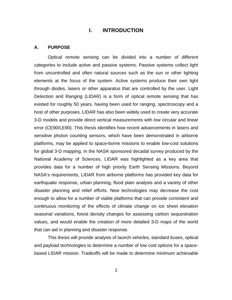
Optical remote sensing can be divided into a number of different
categories to include active and passive systems. Passive systems collect light
from uncontrolled and often natural sources such as the sun or other lighting
elements at the focus of the system. Active systems produce their own light
through diodes, lasers or other apparatus that are controlled by the user. Light
Detection and Ranging (LIDAR) is a form of optical remote sensing that has
existed for roughly 50 years, having been used for ranging, spectroscopy and a
host of other purposes. LIDAR has also been widely used to create very accurate
3-D models and provide direct vertical measurements with low circular and linear
error (CE90/LE90). This thesis identifies how recent advancements in lasers and
sensitive photon counting sensors, which have been demonstrated in airborne
platforms, may be applied to space-borne missions to enable low-cost solutions
for global 3-D mapping. In the NASA sponsored decadal survey produced by the
National Academy of Sciences, LIDAR was highlighted as a key area that
provides data for a number of high priority Earth Sensing Missions. Beyond
NASA’s requirements, LIDAR from airborne platforms has provided key data for
earthquake response, urban planning, flood plain analysis and a variety of other
disaster planning and relief efforts. New technologies may decrease the cost
enough to allow for a number of viable platforms that can provide consistent and
continuous monitoring of the effects of climate change on ice sheet elevation
seasonal variations, forest density changes for assessing carbon sequestration
values, and would enable the creation of more detailed 3-D maps of the world
that can aid in planning and disaster response.
This thesis will provide analysis of launch vehicles, standard buses, optical
and payload technologies to determine a number of low cost options for a space-
based LIDAR mission. Tradeoffs will be made to determine minimum achievable
1
links depending on mission duration, orbital regimes and area coverage rates
with an eye towards mission utility.
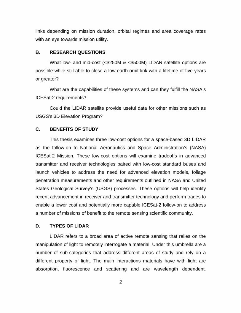
B. RESEARCH QUESTIONS
What low- and mid-cost (<$250M & <$500M) LIDAR satellite options are
possible while still able to close a low-earth orbit link with a lifetime of five years
or greater?
What are the capabilities of these systems and can they fulfill the NASA’s
ICESat-2 requirements?
Could the LIDAR satellite provide useful data for other missions such as
USGS’s 3D Elevation Program?
C. BENEFITS OF STUDY
This thesis examines three low-cost options for a space-based 3D LIDAR
as the follow-on to National Aeronautics and Space Administration’s (NASA)
ICESat-2 Mission. These low-cost options will examine tradeoffs in advanced
transmitter and receiver technologies paired with low-cost standard buses and
launch vehicles to address the need for advanced elevation models, foliage
penetration measurements and other requirements outlined in NASA and United
States Geological Survey’s (USGS) processes. These options will help identify
recent advancement in receiver and transmitter technology and perform trades to
enable a lower cost and potentially more capable ICESat-2 follow-on to address
a number of missions of benefit to the remote sensing scientific community.
D. TYPES OF LIDAR
LIDAR refers to a broad area of active remote sensing that relies on the
manipulation of light to remotely interrogate a material. Under this umbrella are a
number of sub-categories that address different areas of study and rely on a
different property of light. The main interactions materials have with light are
absorption, fluorescence and scattering and are wavelength dependent.
2
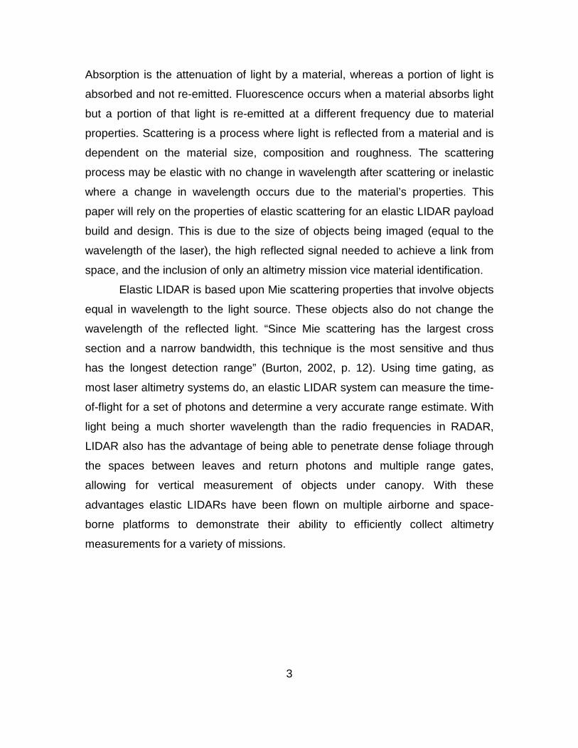
Absorption is the attenuation of light by a material, whereas a portion of light is
absorbed and not re-emitted. Fluorescence occurs when a material absorbs light
but a portion of that light is re-emitted at a different frequency due to material
properties. Scattering is a process where light is reflected from a material and is
dependent on the material size, composition and roughness. The scattering
process may be elastic with no change in wavelength after scattering or inelastic
where a change in wavelength occurs due to the material’s properties. This
paper will rely on the properties of elastic scattering for an elastic LIDAR payload
build and design. This is due to the size of objects being imaged (equal to the
wavelength of the laser), the high reflected signal needed to achieve a link from
space, and the inclusion of only an altimetry mission vice material identification.
Elastic LIDAR is based upon Mie scattering properties that involve objects
equal in wavelength to the light source. These objects also do not change the
wavelength of the reflected light. “Since Mie scattering has the largest cross
section and a narrow bandwidth, this technique is the most sensitive and thus
has the longest detection range” (Burton, 2002, p. 12). Using time gating, as
most laser altimetry systems do, an elastic LIDAR system can measure the time-
of-flight for a set of photons and determine a very accurate range estimate. With
light being a much shorter wavelength than the radio frequencies in RADAR,
LIDAR also has the advantage of being able to penetrate dense foliage through
the spaces between leaves and return photons and multiple range gates,
allowing for vertical measurement of objects under canopy. With these
advantages elastic LIDARs have been flown on multiple airborne and space-
borne platforms to demonstrate their ability to efficiently collect altimetry
measurements for a variety of missions.
3

THIS PAGE INTENTIONALLY LEFT BLANK
4
II. LIDAR OBJECTIVES AND REQUIREMENTS
Direct Detect LIDAR systems provide a unique dataset due to their very
short wavelengths in comparison to RADAR, interferometric synthetic aperture
RADAR and other modes of collecting elevation data. While LIDAR remains a
lower area collection rate platform in comparison to other modalities, the need for
high fidelity elevation measurements has garnered both national and
international government, nonprofit and for-profit support. The National
Academies of Science (NAS) and the United States Geological Survey (USGS)
both commissioned studies that pointed towards the benefits of high fidelity
elevation measurements beyond what is currently available. The NAS performed
the survey in support of future NASA Earth observing satellites, while the USGS
looked at the benefits of terrain elevation data for the nation and its cost saving
capabilities for government, non-government organizations and commercial
applications. This chapter is divided into two sections that cover objectives levied
on NASA by NAS’s Decadal Survey and the USGS’s objectives.
A. NASA OBJECTIVES
Understanding the complex, changing planet on which we live, how it supports life, and how human activities affect its ability to do so in the future is one of the greatest intellectual challenges facing humanity. It is also one of the most important for society as it seeks to achieve prosperity and sustainability. (National Research Council, 2007, p. 1)
In 2004, NASA, NOAA, and the USGS asked the National Research Council to conduct a decadal survey of the Earth sciences community. The charge was to recommend a prioritized list of flight missions and supporting activities for space-based Earth observation over the next decade (through the 2010s) and to identify key factors in planning for the decade beyond (into the 2020s). (Henson, 2008, p. 1)
In the decadal survey, the National Research Council (NRC) came to
consensus on a number of key issues the next generation of Earth observing
satellites should tackle, of which LIDAR was slated as a key technology to 5

provide insight into many of these issues. The scientific questions and
requirements posed to future LIDAR systems centered around five major themes:
glacier and sea ice thickness, vegetation and biomass measurements,
topography, hydrology and atmospheric measurements.
6
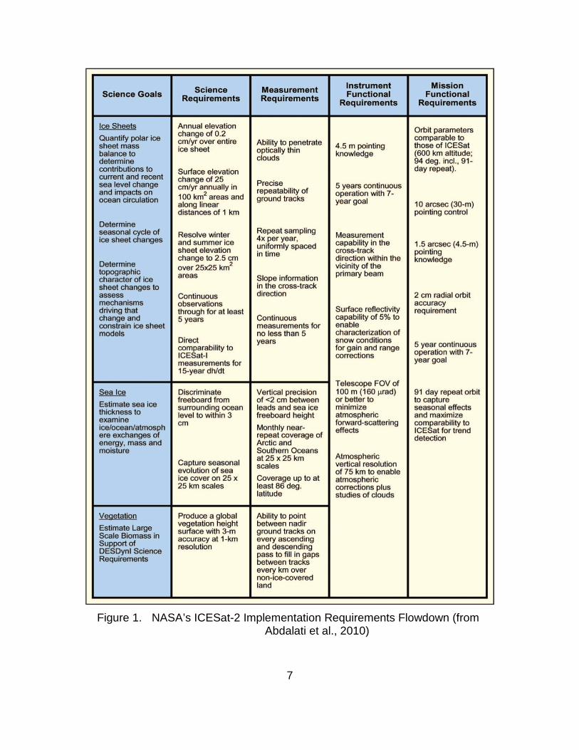
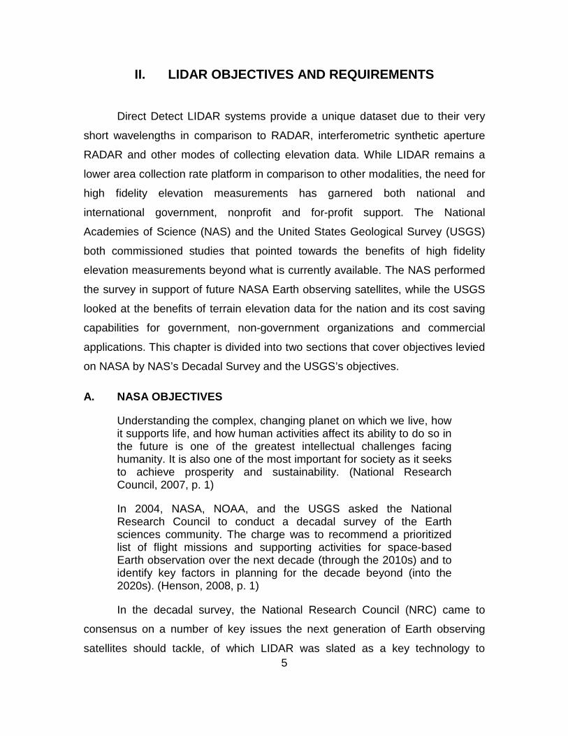
Figure 1. NASA’s ICESat-2 Implementation Requirements Flowdown (from
Abdalati et al., 2010)
7
Science Measurement Instrument Mission Science Goals Requirements Requirements Functional Functional
Requirements Requirements
Ice Sheets Annual elevation Orbit parameters change of 0.2 Quantify polar ice cm/yr over entire Ability to penetrate comparable to
sheet mass 4.5 m pointing those of ICESat balance to
ice sheet optically thin knowledge (600 km altitude; determine clouds 94 deg. incl., 91-contributions to Surface elevation day repeat). current and recent change of 25 sealevel change cm/yr annually in Precise 5 years continuous and impacts on
1 00 km2 areas and repeatability of operation with 7-
ocean circulation along linear
ground tracks year goal 10 arcsec (30-m) distances of 1 km pointing control
Determine seasonal cycle of Resolve winter Repeat sampling
Measurement ice sheet changes and summer ice 4x per year,
capability in the 1.5 arcsec (4.5-m) uniformly spaced sheet elevation in time cross-track pointing change to 2.5 em direction within the knowledge
Determine over 25x25 km2 vicinity of the topographic areas Slope information
primary beam character of ice sheet changes to in the cross-track assess Continuous direction 2 em radial orbit mechanisms observations accuracy driving that through for at least Surface reflectivity requirement change and 5 years Continuous capability of 5% to constrain ice sheet measurements for enable models no less than 5 characterization of
Direct years snow conditions 5 year continuous comparability to for gain and range ICESat-1 corrections operation with 7-
measurements for year goal
15-year dh/dt
Telescope FOV of Sea Ice Discriminate Vertical precision 100m (160 wad) 91 day repeat orbit
Estimate sea ice freeboard from of <2 em between or better to to capture surrounding ocean leads and sea ice minimize seasonal effects
thickness to level to within 3 freeboard height atmospheric and maximize examine em forward-scattering comparability to ice/ocean/atmosph Monthly near- effects ICESat for trend ere exchanges of repeat coverage of detection energy, mass and Arctic and moisture Southern Oceans
Capture seasonal at 25 x 25 km Atmospheric scales vertical resolution
evolution of sea of 75 km to enable ice cover on 25 x Coverage up to at atmospheric 25 km scales least 86 deg. corrections plus
latitude studies of clouds
Vegetation Produce a global Ability to point
Estimate Large vegetation height between nadir surface with 3-m ground tracks on
Scale Biomass in accuracy at 1-km every ascending Support of resolution and descending DESDynl Science pass to fill in gaps Requirements between tracks
every km over non-ice-covered land
1. Glacier, Sea Ice and Ice Sheet Thickness
Mass balance of Earth’s great ice sheets and their contributions to sea level are key issues in climate variability and change. The relationships between sea level and climate have been identified as critical subjects of study in the Intergovernmental Panel on Climate Change assessments, the Climate Change Science Program strategy, and the U.S. International Earth Observing System. Because much of the behavior of ice sheets is manifested in their shape, accurate observations of ice elevation changes are essential for understanding ice sheets’ current and likely contributions to sea-level rise. (National Research Council, 2007, p. 271)
The launch of ICESat-1 in 2003 in addition to other missions over the
polar cryosphere have helped inform the scientific community about the impact of
climate change over the past decade. With nearly 75% of the Earth’s freshwater
contained in ice sheets and glaciers, scientists and climatologists have examined
the extent of ice loss and potential effects on the environment and society. Past
data suggests that “The Greenland and Antarctic ice sheets are losing mass at
an increasing rate [1]–[3]… The sea ice that covers the Arctic Ocean has
decreased in areal extent far more rapidly than climate models have predicted [8]
and has thinned substantially [9], suggesting that a summertime ice-free Arctic
ocean may be imminent” (Abdalati et al., 2010, p. 736).
The requirements placed on ICESat-2 build upon lessons learned from
measurements taken from the ICESat-1 mission. An assessment of the ICESat-1
data showed that the accuracy of its thickness measurements were within half a
meter of measurements based upon submarine sonar and ocean moorings
(Abdalati et al., 2010). To improve this even further scientists gathered for the
ICESat-2 Workshop where they set priorities in three major sea ice areas:
“Improve current knowledge of mean and variability of the ice thickness
distribution of the polar oceans, provide long-term monitoring to determine trends
in ice thickness, and refine the estimates of sea ice outflow into the Northern
Atlantic” (NASA, 2007, p. 12). To accomplish these missions, more stringent
requirements were needed, driving the ICESat-2 mission to a 2-cm range
8

precision (satellite-to-surface) and a pointing knowledge of less than 2
arcseconds (equating to roughly six meters horizontally). The added pointing and
range precision combined with a longer expected lifetime and continuous
campaigns (versus the 33-day campaigns on ICESat-1 due to laser issues) will
enable seasonal ice sheet measurement accuracies of ±2 cm and yearly
accuracies of ±1cm/year. Overall, these numbers equate to an uncertainty of
about ten percent of the annual ice sheet mass interchange with the ocean,
resulting in an accuracy of ±1mm/year of sea level rise (NASA, 2007).
2. Vegetation and Biomass
The horizontal and vertical structure of ecosystems is a key feature that enables quantification of carbon storage, the effects of disturbances such as fire, and species habitats. The above ground woody biomass and its associated below ground biomass store a large pool of terrestrial carbon. Quantifying changes in the size of this pool, its horizontal distribution, and its vertical structure resulting from natural and human-induced perturbations such as deforestation and fire, as well as the recovery processes, is critical for quantifying ecosystem change. (National Research Council, 2007, p. 191)
In addition to studying the cryosphere, NASA’s Decadal Survey and the
ICESat-2 Workshop identified the need to study changes in biomass ecosystem
structure to estimate land carbon storage. The carbon contained in Earth’s forest
canopies account for roughly 85% of all aboveground biomass, playing a
significant role in terrestrial carbon stocks. Due to the dynamic nature of forest
carbon stocks (e.g., fire, logging, regrowth, disease), three-dimensional
measurements of the structure of forests and their canopy heights are needed to
accurately estimate varying biomass and carbon stocks and better understand
the carbon cycle. “These measurements include vegetation height; the vertical
profile of canopy elements (i.e., leaves, stems, and branches); and/or the volume
scattering of canopy elements. Such measurements are critical for reducing
uncertainties in the global carbon budget” (NASA, 2007, p. 14). Three-
dimensional measurements of vegetation are also important for the mapping of
9

forest disease and pest outbreaks, and to characterize animal habitats and
biodiversity changes due to anthropogenic disturbances. Requirements for the
ICESat-2 mission have been increased over those of ICESat-1 to help answer
many of the questions surrounding these issues. The specific vegetation
requirement of a three-meter vertical accuracy with a 1 km spatial resolution of
the Earth’s canopy was taken from a more stringent set of requirements from the
Vegetation Structure Science Working Group:
…statistically rigorous sampling of height and profiles and/or contiguous global coverage over a 3-year period … maximum vertical height measurement accuracy ~1m, vertical resolution of canopy profile, 2–3 m, 25 m spatial resolution or better in a sampling mode; aboveground biomass and changes including disturbance; spatial resolution ~100 m to 1 km for contiguous biomass.” (NASA, 2007, p. 15)
3. Topography
Earth’s surface is dynamic in the literal sense: it is continually being shaped by the interplay of uplift, erosion, and deposition as modulated by hydrological and biological processes. Surface topography influences air currents and precipitation patterns and controls how water and soil are distributed across the landscape… And it influences how natural hazards, such as landslides, floods, and earthquakes, are distributed across the landscape. (National Research Council, 2007, p. 119)
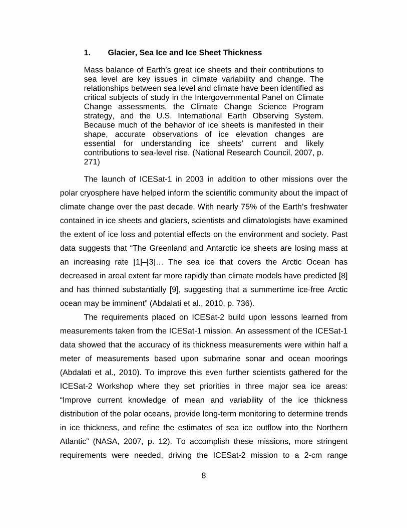
While only a tertiary mission for the ICESat-2 spacecraft, advanced
topographic information from LIDAR systems is valued due to the lack of high-
resolution data currently available. Worldwide topographical maps generated by
the Shuttle Radar Topography Mission remain the main dataset for terrain maps
and only have post-spacing of 30 to 90 meters. At this resolution, multiple
features are obscured that are beneficial to understanding and calculating
surface topographic effects for a number of phenomena (as can be seen in
Figure 2). Higher resolution data at 5-m post-spacing and sub-10cm precision
would enable advanced analysis of a number of geological, topographical and
geomorphological processes to include prediction of potential landslides, floods,
tsunami effects, volcanic and mud flows and earthquakes. These predictions, 10
informed by advanced topographic data, would help in disaster mitigation,
planning and relief operations that could save lives and money (National
Research Council, 2007).
The events of the past few years, for example, the volcanic unrest of Mt. Saint Helens in 2004, the devastation of the December 26, 2004, Sumatra earthquake and resulting tsunami, the loss of life and destruction from the great Pakistan earthquake and associated landslides of 2005, and the chaos following Hurricane Katrina… demonstrate humankind’s vulnerability to naturally occurring disasters. These events highlighted the costs associated with inadequate information and the consequences of inadequate planning for the dissemination of available or obtainable information. (National Research Council, 2007, pp. 223–4)
Figure 2. DEM Comparison of California’s Salinas River (from National
Research Council, 2007)
11
4. Hydrology and Atmospheric Sensing
Two additional missions for ICESat-2 that have also been levied on past
and future LIDAR systems are the monitoring of hydrological and atmospheric
phenomenon. Specifically, measurements of lakes and reservoirs at 10-cm
vertical accuracy in 1-week intervals would generate “improved knowledge of
global water cycle science and also enhance decision making in a number of
applications including water resources, agriculture, disaster management, and
public health” (NASA, 2007, p. 18). For atmospheric science, ICESat-1
demonstrated the utility of the 1064-nm channel at detecting a number of
important characteristics to include: “polar clouds and haze, global pollution
aerosols, planetary boundary layer height, [and] global cloud change
monitoring” (NASA, 2007, p. 18). While the ICESat-II Workshop and other groups
provided no requirements in regards to atmospheric monitoring, it remains a
potential capability for future LIDAR-based system to include ICESat-2.
B. USGS’S NATIONAL ENHANCED ELEVATION ASSESSMENT
For much of the nation, professionals in a broad range of critical fields find themselves lacking the right data to perform their missions. Today, federal agencies, states, local governments, tribes and nongovernmental users (not-for-profit and private businesses) are grappling with maps created from elevation data that are mostly 30–50 years old and far less detailed than is needed. (Dewberry, 2012, p. 34)
In December of 2011, the USGS sponsored the National Enhanced
Elevation Assessment (NEEA) “[t]o develop strategies to better meet national
elevation data needs…(1) document national-level requirements for improved
elevation data, (2) estimate the benefits and costs of meeting those
requirements, and (3) evaluate new, national-level elevation program models”
(Snyder, 2013, p. 105). The study reached a number of conclusions about the
benefits of enhanced elevation data to public, private and nonprofits, having
determined a potential benefit of $13 billion annually. The participants included a
variety of government and non-governmental organizations that documented 602
12
mission-critical activities that require more accurate data than is available today.
Among these activities are optimized precision agriculture, flood risk analysis,
improved navigation for airborne and terrestrial assets, wildfire prevention and
mitigation, wind farm planning and optimization and fuel consumption reduction
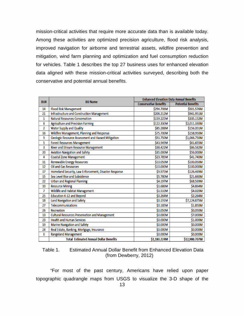
for vehicles. Table 1 describes the top 27 business uses for enhanced elevation
data aligned with these mission-critical activities surveyed, describing both the
conservative and potential annual benefits.
Table 1. Estimated Annual Dollar Benefit from Enhanced Elevation Data
(from Dewberry, 2012)
“For most of the past century, Americans have relied upon paper
topographic quadrangle maps from USGS to visualize the 3-D shape of the 13
topography by human interpretation of contour lines manually compiled by labor-
intensive photogrammetric processes” (Dewberry, 2012, p. 1). LIDAR has
significantly changed the way USGS has derived high-resolution elevation data
for public use. Currently the National Elevation Dataset (NED) contains LIDAR
over roughly 28 percent of the lower 49 states and continues at a rate of 2–3
percent per year. At this rate, full U.S. coverage is anticipated to take 35 years,
negating the full benefits outlined in the study and spurring on the need for a
comprehensive plan to address the nation’s enhanced elevation needs.
Airborne LIDAR and Interferometric Synthetic Aperture RADAR (IFSAR)
are the most widely used methods used to collect high-resolution elevation data.
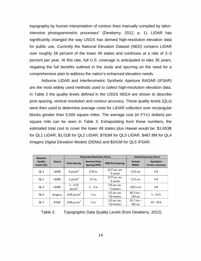
In Table 2 the quality levels defined in the USGS NEEA are shown to describe
post spacing, vertical resolution and contour accuracy. These quality levels (QLs)
were then used to determine average costs for LIDAR collection over rectangular
blocks greater than 5,000 square miles. The average cost (in FY11 dollars) per
square mile can be seen in Table 3. Extrapolating from these numbers, the
estimated total cost to cover the lower 48 states plus Hawaii would be: $1.653B
for QL1 LIDAR, $1.01B for QL2 LIDAR, $763M for QL3 LIDAR, $487.8M for QL4
Imagery Digital Elevation Models (DEMs) and $241M for QL5 IFSAR.
Table 2. Topographic Data Quality Levels (from Dewberry, 2012)
14
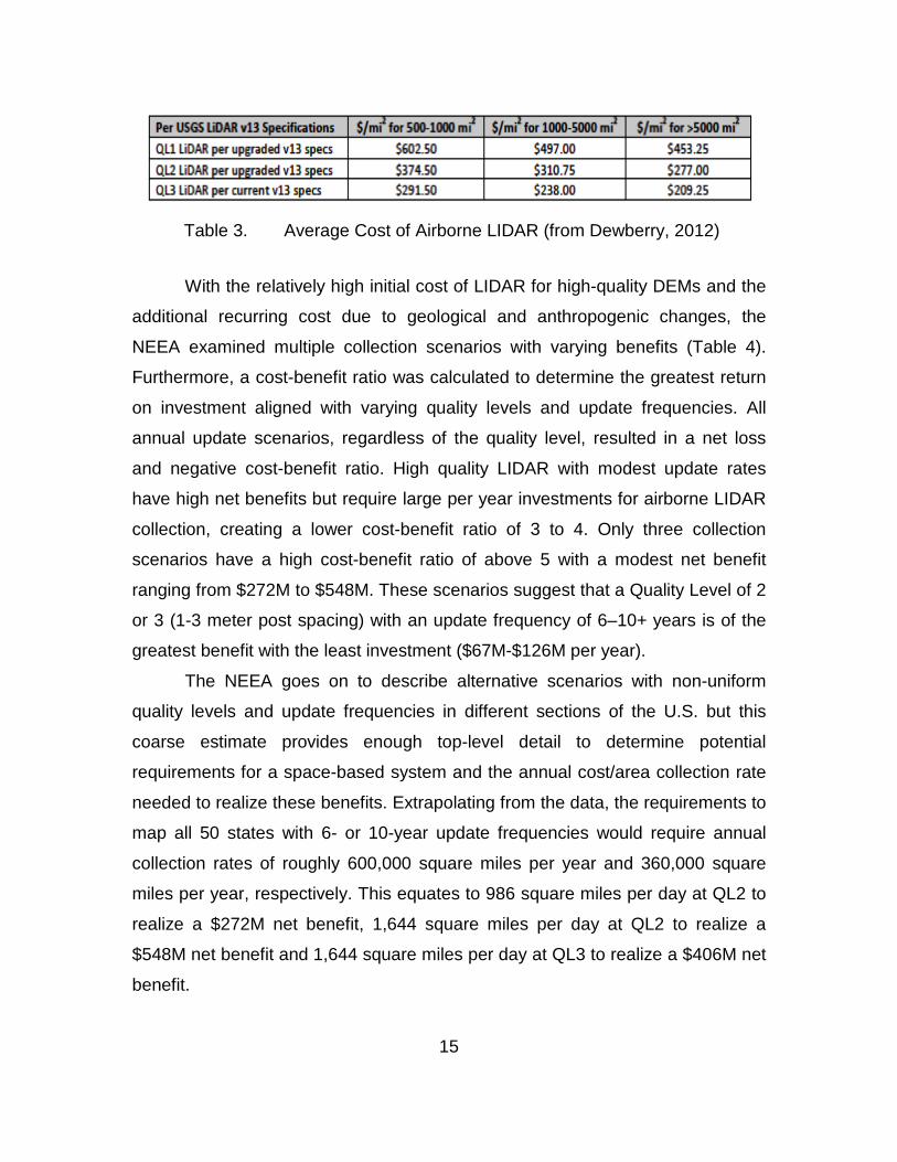
Table 3. Average Cost of Airborne LIDAR (from Dewberry, 2012)
With the relatively high initial cost of LIDAR for high-quality DEMs and the
additional recurring cost due to geological and anthropogenic changes, the
NEEA examined multiple collection scenarios with varying benefits (Table 4).
Furthermore, a cost-benefit ratio was calculated to determine the greatest return
on investment aligned with varying quality levels and update frequencies. All
annual update scenarios, regardless of the quality level, resulted in a net loss
and negative cost-benefit ratio. High quality LIDAR with modest update rates
have high net benefits but require large per year investments for airborne LIDAR
collection, creating a lower cost-benefit ratio of 3 to 4. Only three collection
scenarios have a high cost-benefit ratio of above 5 with a modest net benefit
ranging from $272M to $548M. These scenarios suggest that a Quality Level of 2
or 3 (1-3 meter post spacing) with an update frequency of 6–10+ years is of the
greatest benefit with the least investment ($67M-$126M per year).
The NEEA goes on to describe alternative scenarios with non-uniform
quality levels and update frequencies in different sections of the U.S. but this
coarse estimate provides enough top-level detail to determine potential
requirements for a space-based system and the annual cost/area collection rate
needed to realize these benefits. Extrapolating from the data, the requirements to
map all 50 states with 6- or 10-year update frequencies would require annual
collection rates of roughly 600,000 square miles per year and 360,000 square
miles per year, respectively. This equates to 986 square miles per day at QL2 to
realize a $272M net benefit, 1,644 square miles per day at QL2 to realize a
$548M net benefit and 1,644 square miles per day at QL3 to realize a $406M net
benefit.
15
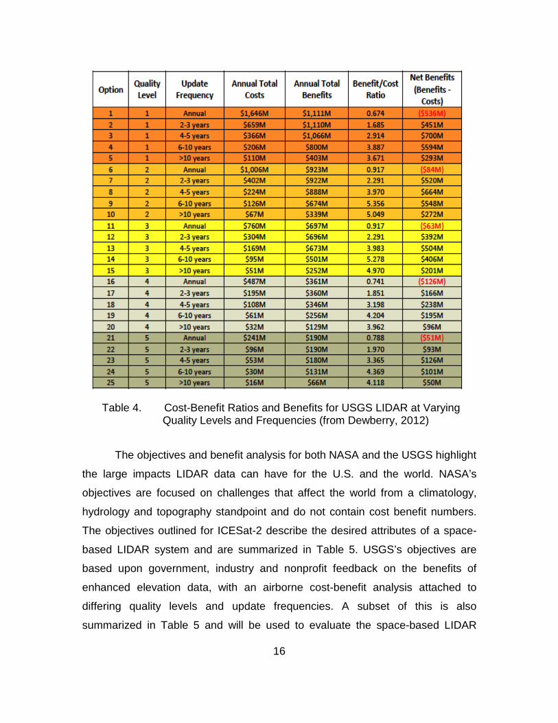
Table 4. Cost-Benefit Ratios and Benefits for USGS LIDAR at Varying
Quality Levels and Frequencies (from Dewberry, 2012)
The objectives and benefit analysis for both NASA and the USGS highlight
the large impacts LIDAR data can have for the U.S. and the world. NASA’s
objectives are focused on challenges that affect the world from a climatology,
hydrology and topography standpoint and do not contain cost benefit numbers.
The objectives outlined for ICESat-2 describe the desired attributes of a space-
based LIDAR system and are summarized in Table 5. USGS’s objectives are
based upon government, industry and nonprofit feedback on the benefits of
enhanced elevation data, with an airborne cost-benefit analysis attached to
differing quality levels and update frequencies. A subset of this is also
summarized in Table 5 and will be used to evaluate the space-based LIDAR
16
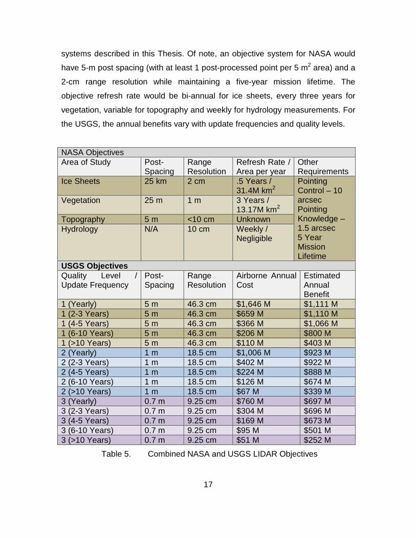
systems described in this Thesis. Of note, an objective system for NASA would
have 5-m post spacing (with at least 1 post-processed point per 5 m2 area) and a
2-cm range resolution while maintaining a five-year mission lifetime. The
objective refresh rate would be bi-annual for ice sheets, every three years for
vegetation, variable for topography and weekly for hydrology measurements. For
the USGS, the annual benefits vary with update frequencies and quality levels.
NASA Objectives Area of Study Post-
Spacing Range Resolution
Refresh Rate / Area per year
Other Requirements
Ice Sheets 25 km 2 cm .5 Years / 31.4M km2
Pointing Control – 10 arcsec Pointing Knowledge – 1.5 arcsec 5 Year Mission Lifetime
Vegetation 25 m 1 m 3 Years / 13.17M km2
Topography 5 m <10 cm Unknown Hydrology N/A 10 cm Weekly /
Negligible
USGS Objectives Quality Level / Update Frequency
Post-Spacing
Range Resolution
Airborne Annual Cost
Estimated Annual Benefit
1 (Yearly) 5 m 46.3 cm $1,646 M $1,111 M 1 (2-3 Years) 5 m 46.3 cm $659 M $1,110 M 1 (4-5 Years) 5 m 46.3 cm $366 M $1,066 M 1 (6-10 Years) 5 m 46.3 cm $206 M $800 M 1 (>10 Years) 5 m 46.3 cm $110 M $403 M 2 (Yearly) 1 m 18.5 cm $1,006 M $923 M 2 (2-3 Years) 1 m 18.5 cm $402 M $922 M 2 (4-5 Years) 1 m 18.5 cm $224 M $888 M 2 (6-10 Years) 1 m 18.5 cm $126 M $674 M 2 (>10 Years) 1 m 18.5 cm $67 M $339 M 3 (Yearly) 0.7 m 9.25 cm $760 M $697 M 3 (2-3 Years) 0.7 m 9.25 cm $304 M $696 M 3 (4-5 Years) 0.7 m 9.25 cm $169 M $673 M 3 (6-10 Years) 0.7 m 9.25 cm $95 M $501 M 3 (>10 Years) 0.7 m 9.25 cm $51 M $252 M
Table 5. Combined NASA and USGS LIDAR Objectives
17

THIS PAGE INTENTIONALLY LEFT BLANK
18
III. HISTORY OF LIDAR IN SPACE
A number of methods have historically been developed and used to
measure the distance to an object. Initial technologies included RADAR and
research into microwave technologies. Limitations were identified due to the
wavelength used and the need for higher frequencies to increase resolution and
distance accuracy. As scientists and engineers continued to press to find
solutions in the microwave domain, a key contribution to the field came on 6
August 1960 when Theodore Maiman “proposed a technique for the generation
of very monochromatic radiation in the infra-red optical region of the spectrum”
(Maiman, p. 494). The ability to generate narrow wavelengths of light led to the
invention of the LASER or “Light Amplification by Simulated Emission of
Radiation.” Shortly thereafter, Hughes Laboratories introduced the first LASER
rangefinder, increasing the accuracy of the measurement of an object’s three
dimensional position nearly 1000 times over radar systems of the same time
period. Since then, these rangefinders have found their way into defense
systems, video game consoles and golf pro shops around the world, and have
paved the way for LIDAR mapping technologies.
With the invention of LIDAR for laser altimetry, LIDAR systems have found
their way into multiple applications aboard ground vehicles, aircraft, helicopters,
ships and even satellites. In the space environment, NASA has been a pioneer in
developing laser rangefinders for docking and laser altimeters for measuring
surface characteristics of different celestial bodies. NASA’s accomplishments in
space-based LIDAR are numerous and range from Apollo 15 through the present
day.
A. APOLLO LASER ALTIMETER
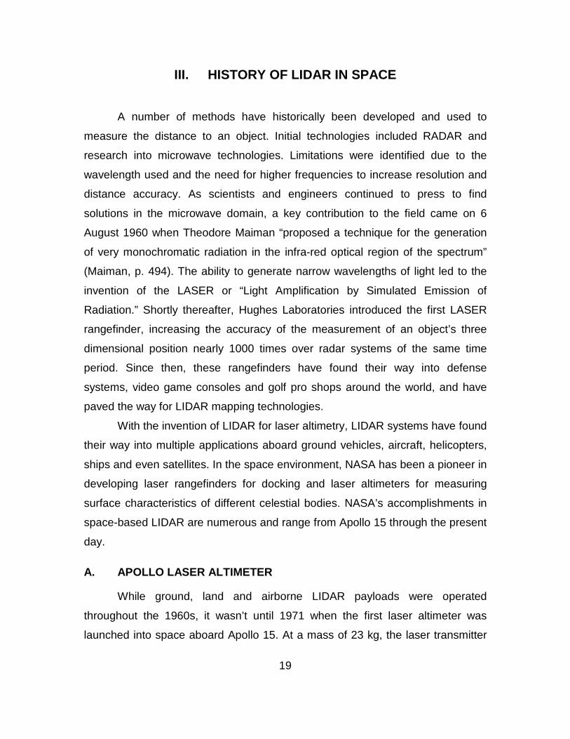
While ground, land and airborne LIDAR payloads were operated
throughout the 1960s, it wasn’t until 1971 when the first laser altimeter was
launched into space aboard Apollo 15. At a mass of 23 kg, the laser transmitter
19
utilized a mechanically Q-switched and flash pumped ruby laser. The design was
based upon a military qualified rangefinder for tank applications and adapted to
the rigors of space. With a pulse repetition frequency of 0.05 Hz, the payload
mapped portions of the moon with a post spacing of 30 kilometers and accuracy
of nearly 10 meters. The full collection only lasted for roughly 5,000 shots, but the
Apollo laser altimeter proved the worth of lasers for topographic applications
(Masursky, Colton, El-Baz, & Doyle, 1978).
Figure 3. 1971 Apollo Laser Altimeter (from Abshire, 2010)
B. CLEMENTINE
The laser community continued to make advances in advanced lasing
mediums, eventually replacing the ruby laser with a number of other solid-state
and new chemical vapor lasers. Due to the difficulty of ruggedizing a chemical
vapor laser for space due to launch survival and outgassing issues, solid-state
lasers (primarily Nd:YAG) gained greater traction in the space LIDAR community.
The Nd:YAG laser continues to be the standard for space-based solid-state
LIDAR lasers, introduced during the Clementine and NEAR missions and having
demonstrated roughly 600,000 and 11 million shots, respectively (Neumann,
2001).
20
The first space-based use of Nd:YAG lasers occurred on the Clementine
mission, launched on 25 January 1994. The mission was a joint venture between
Ballistic Missile Defense Organization (BMDO) and NASA, and sought to
demonstrate new spacecraft systems and technologies in a high-radiation, lunar
orbit, as well as provide detailed topographic, altimetry and multispectral data of
the moon. One of the new technologies on-board was the Nd:YAG miniature
LIDAR. Clementine’s laser altimeter performed substantially better than Apollo
missions 15, 16, and 17, whose ruby laser only lasted roughly 7,080 shots over
all three missions. Clementine saw a two orders of magnitude improvement over
Apollo’s ruby lasers, firing for roughly 600,000 shots (Neumann, 2001).
Clementine’s LIDAR payload consisted of a diode-pumped Cr:Nd:YAG
laser operating at both 1064nm (ranging) and 532nm (active imaging) and a
silicon avalanche photodiode (SiAPD). In a 425km x 8300 km highly elliptical
polar orbit, the 1.1 kg payload collected data every 2 km along-track (Spudis,
1994). The spot size or instantaneous field of view (IFOV) was 100 meters with a
90-meter vertical accuracy and 40-meter range resolution (Neumann, 2001). The
laser operated at 1 Hz with a 10-nanosecond pulse-width providing 180 mJ per
pulse or with a thermal-limited burst rate of 400 pulses at 8 Hz. Though the
vertical precision and accuracy of the Clementine LIDAR system was relatively
poor, the improvement of Nd:YAG laser lifetimes and reduced mass over that of
the Apollo ruby lasers paved the way for future Nd:YAG-based LIDAR systems in
space (Sorensen & Spudis, 2005).
21
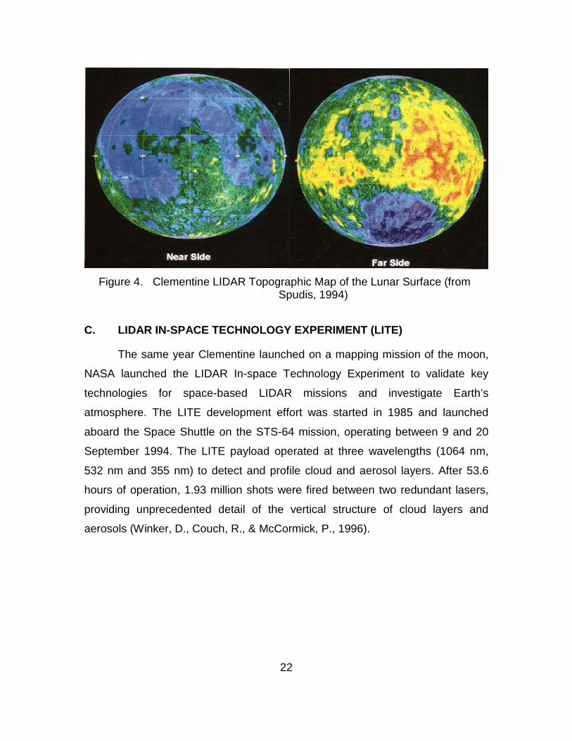
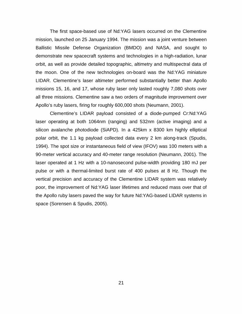
Figure 4. Clementine LIDAR Topographic Map of the Lunar Surface (from
Spudis, 1994)
C. LIDAR IN-SPACE TECHNOLOGY EXPERIMENT (LITE)
The same year Clementine launched on a mapping mission of the moon,
NASA launched the LIDAR In-space Technology Experiment to validate key
technologies for space-based LIDAR missions and investigate Earth’s
atmosphere. The LITE development effort was started in 1985 and launched
aboard the Space Shuttle on the STS-64 mission, operating between 9 and 20
September 1994. The LITE payload operated at three wavelengths (1064 nm,
532 nm and 355 nm) to detect and profile cloud and aerosol layers. After 53.6
hours of operation, 1.93 million shots were fired between two redundant lasers,
providing unprecedented detail of the vertical structure of cloud layers and
aerosols (Winker, D., Couch, R., & McCormick, P., 1996).
22
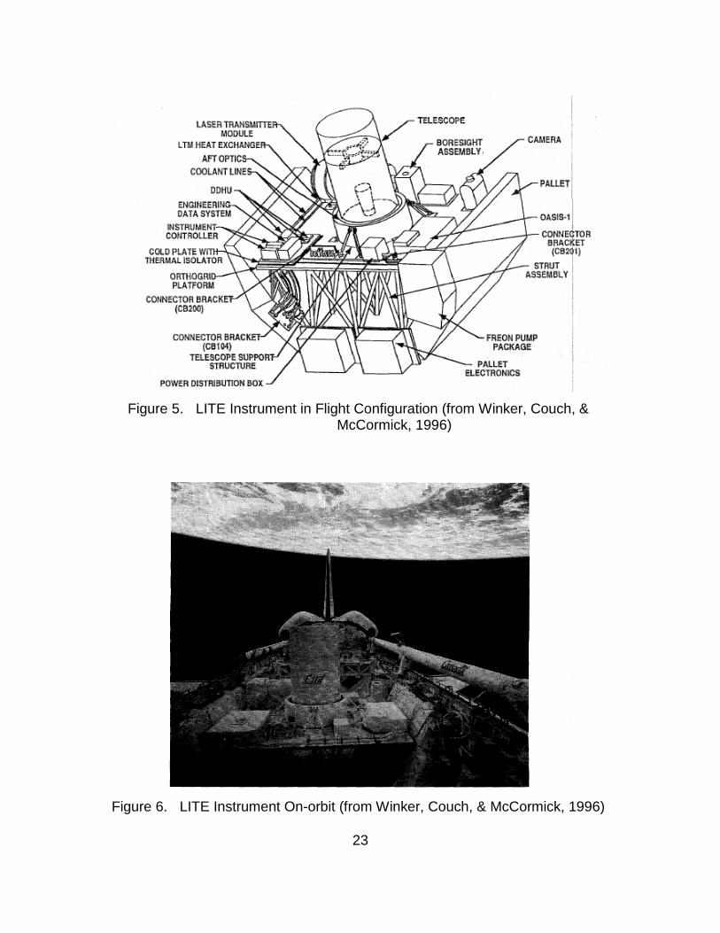
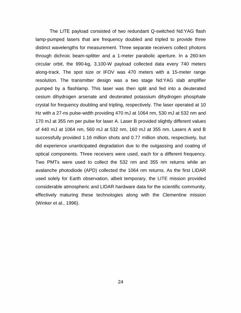
Figure 5. LITE Instrument in Flight Configuration (from Winker, Couch, &
McCormick, 1996)
Figure 6. LITE Instrument On-orbit (from Winker, Couch, & McCormick, 1996)
23
The LITE payload consisted of two redundant Q-switched Nd:YAG flash
lamp-pumped lasers that are frequency doubled and tripled to provide three
distinct wavelengths for measurement. Three separate receivers collect photons
through dichroic beam-splitter and a 1-meter parabolic aperture. In a 260-km
circular orbit, the 990-kg, 3,100-W payload collected data every 740 meters
along-track. The spot size or IFOV was 470 meters with a 15-meter range
resolution. The transmitter design was a two stage Nd:YAG slab amplifier
pumped by a flashlamp. This laser was then split and fed into a deuterated
cesium dihydrogen arsenate and deuterated potassium dihydrogen phosphate
crystal for frequency doubling and tripling, respectively. The laser operated at 10
Hz with a 27-ns pulse-width providing 470 mJ at 1064 nm, 530 mJ at 532 nm and
170 mJ at 355 nm per pulse for laser A. Laser B provided slightly different values
of 440 mJ at 1064 nm, 560 mJ at 532 nm, 160 mJ at 355 nm. Lasers A and B
successfully provided 1.16 million shots and 0.77 million shots, respectively, but
did experience unanticipated degradation due to the outgassing and coating of
optical components. Three receivers were used, each for a different frequency.
Two PMTs were used to collect the 532 nm and 355 nm returns while an
avalanche photodiode (APD) collected the 1064 nm returns. As the first LIDAR
used solely for Earth observation, albeit temporary, the LITE mission provided
considerable atmospheric and LIDAR hardware data for the scientific community,
effectively maturing these technologies along with the Clementine mission
(Winker et al., 1996).
24
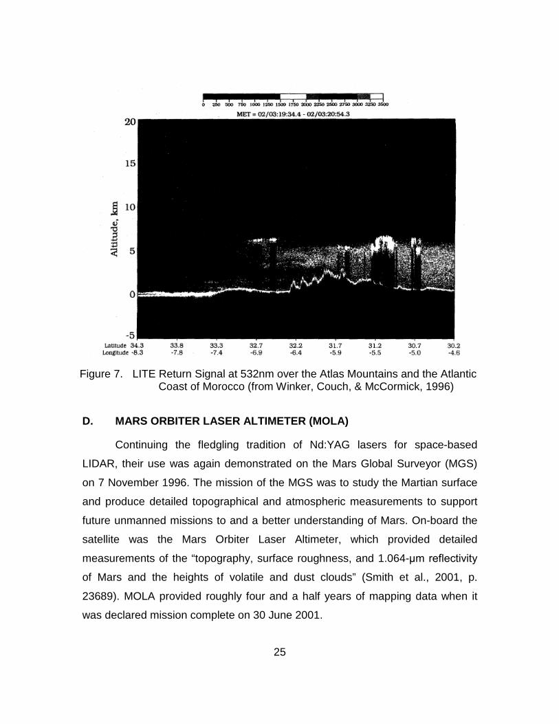
Figure 7. LITE Return Signal at 532nm over the Atlas Mountains and the Atlantic
Coast of Morocco (from Winker, Couch, & McCormick, 1996)
D. MARS ORBITER LASER ALTIMETER (MOLA)
Continuing the fledgling tradition of Nd:YAG lasers for space-based
LIDAR, their use was again demonstrated on the Mars Global Surveyor (MGS)
on 7 November 1996. The mission of the MGS was to study the Martian surface
and produce detailed topographical and atmospheric measurements to support
future unmanned missions to and a better understanding of Mars. On-board the
satellite was the Mars Orbiter Laser Altimeter, which provided detailed
measurements of the “topography, surface roughness, and 1.064-μm reflectivity
of Mars and the heights of volatile and dust clouds” (Smith et al., 2001, p.
23689). MOLA provided roughly four and a half years of mapping data when it
was declared mission complete on 30 June 2001.
25
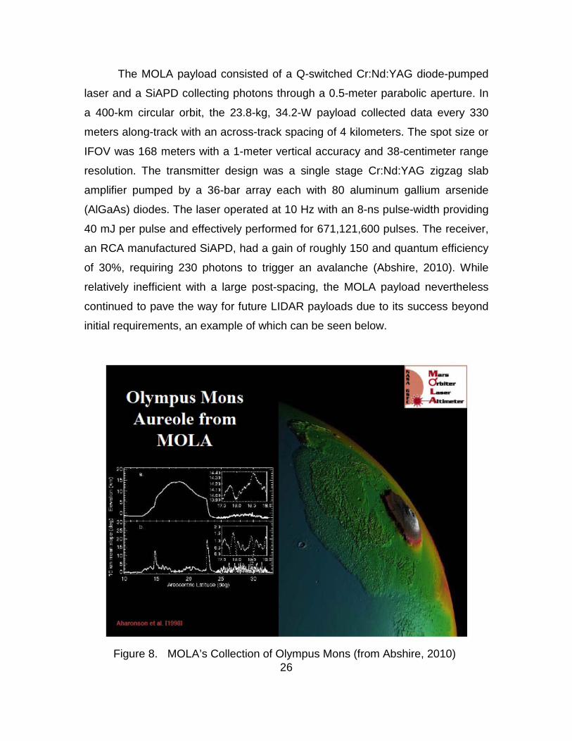
The MOLA payload consisted of a Q-switched Cr:Nd:YAG diode-pumped
laser and a SiAPD collecting photons through a 0.5-meter parabolic aperture. In
a 400-km circular orbit, the 23.8-kg, 34.2-W payload collected data every 330
meters along-track with an across-track spacing of 4 kilometers. The spot size or
IFOV was 168 meters with a 1-meter vertical accuracy and 38-centimeter range
resolution. The transmitter design was a single stage Cr:Nd:YAG zigzag slab
amplifier pumped by a 36-bar array each with 80 aluminum gallium arsenide
(AlGaAs) diodes. The laser operated at 10 Hz with an 8-ns pulse-width providing
40 mJ per pulse and effectively performed for 671,121,600 pulses. The receiver,
an RCA manufactured SiAPD, had a gain of roughly 150 and quantum efficiency
of 30%, requiring 230 photons to trigger an avalanche (Abshire, 2010). While
relatively inefficient with a large post-spacing, the MOLA payload nevertheless
continued to pave the way for future LIDAR payloads due to its success beyond
initial requirements, an example of which can be seen below.
Figure 8. MOLA’s Collection of Olympus Mons (from Abshire, 2010)
26
E. MESSENGER LASER ALTIMETER (MLA)
The MESSENGER spacecraft followed on the heels of MOLA’s
successes, having launched on 3 August 2004 from Kennedy Space Center. As
the first spacecraft to orbit Mercury, MESSENGER’s mission was to characterize
the geological composition and history of the innermost planet, as well as answer
fundamental questions of how the planet was formed. The MLA was one of
seven instruments on-board the spacecraft, which provided detailed topographic
and reflectivity measurements of Mercury. MESSENGER continues to provide
data on Mercury since its orbital insertion on 17 March 2011 to present day
operations with over 26,716,501 laser shots to date (C. Ernst, personal
communication, November 5, 2013).
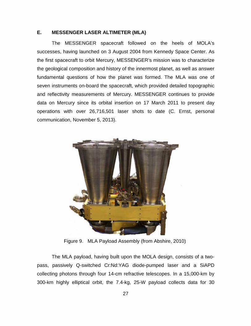
Figure 9. MLA Payload Assembly (from Abshire, 2010)
The MLA payload, having built upon the MOLA design, consists of a two-
pass, passively Q-switched Cr:Nd:YAG diode-pumped laser and a SiAPD
collecting photons through four 14-cm refractive telescopes. In a 15,000-km by
300-km highly elliptical orbit, the 7.4-kg, 25-W payload collects data for 30
27
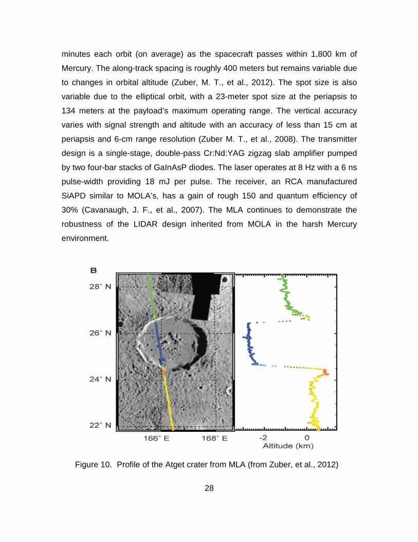
minutes each orbit (on average) as the spacecraft passes within 1,800 km of
Mercury. The along-track spacing is roughly 400 meters but remains variable due
to changes in orbital altitude (Zuber, M. T., et al., 2012). The spot size is also
variable due to the elliptical orbit, with a 23-meter spot size at the periapsis to
134 meters at the payload’s maximum operating range. The vertical accuracy
varies with signal strength and altitude with an accuracy of less than 15 cm at
periapsis and 6-cm range resolution (Zuber M. T., et al., 2008). The transmitter
design is a single-stage, double-pass Cr:Nd:YAG zigzag slab amplifier pumped
by two four-bar stacks of GaInAsP diodes. The laser operates at 8 Hz with a 6 ns
pulse-width providing 18 mJ per pulse. The receiver, an RCA manufactured
SiAPD similar to MOLA’s, has a gain of rough 150 and quantum efficiency of
30% (Cavanaugh, J. F., et al., 2007). The MLA continues to demonstrate the
robustness of the LIDAR design inherited from MOLA in the harsh Mercury
environment.
Figure 10. Profile of the Atget crater from MLA (from Zuber, et al., 2012)
28
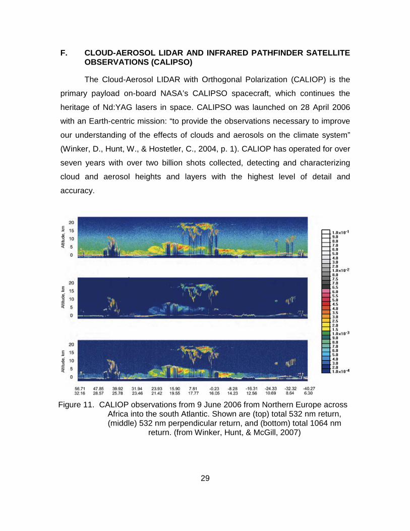
F. CLOUD-AEROSOL LIDAR AND INFRARED PATHFINDER SATELLITE OBSERVATIONS (CALIPSO)
The Cloud-Aerosol LIDAR with Orthogonal Polarization (CALIOP) is the
primary payload on-board NASA’s CALIPSO spacecraft, which continues the
heritage of Nd:YAG lasers in space. CALIPSO was launched on 28 April 2006
with an Earth-centric mission: “to provide the observations necessary to improve
our understanding of the effects of clouds and aerosols on the climate system”
(Winker, D., Hunt, W., & Hostetler, C., 2004, p. 1). CALIOP has operated for over
seven years with over two billion shots collected, detecting and characterizing
cloud and aerosol heights and layers with the highest level of detail and
accuracy.
Figure 11. CALIOP observations from 9 June 2006 from Northern Europe across
Africa into the south Atlantic. Shown are (top) total 532 nm return, (middle) 532 nm perpendicular return, and (bottom) total 1064 nm
return. (from Winker, Hunt, & McGill, 2007)
29
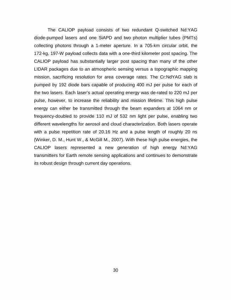
The CALIOP payload consists of two redundant Q-switched Nd:YAG
diode-pumped lasers and one SiAPD and two photon multiplier tubes (PMTs)
collecting photons through a 1-meter aperture. In a 705-km circular orbit, the
172-kg, 197-W payload collects data with a one-third kilometer post spacing. The
CALIOP payload has substantially larger post spacing than many of the other
LIDAR packages due to an atmospheric sensing versus a topographic mapping
mission, sacrificing resolution for area coverage rates. The Cr:NdYAG slab is
pumped by 192 diode bars capable of producing 400 mJ per pulse for each of
the two lasers. Each laser’s actual operating energy was de-rated to 220 mJ per
pulse, however, to increase the reliability and mission lifetime. This high pulse
energy can either be transmitted through the beam expanders at 1064 nm or
frequency-doubled to provide 110 mJ of 532 nm light per pulse, enabling two
different wavelengths for aerosol and cloud characterization. Both lasers operate
with a pulse repetition rate of 20.16 Hz and a pulse length of roughly 20 ns
(Winker, D. M., Hunt W., & McGill M., 2007). With these high pulse energies, the
CALIOP lasers represented a new generation of high energy Nd:YAG
transmitters for Earth remote sensing applications and continues to demonstrate
its robust design through current day operations.
30
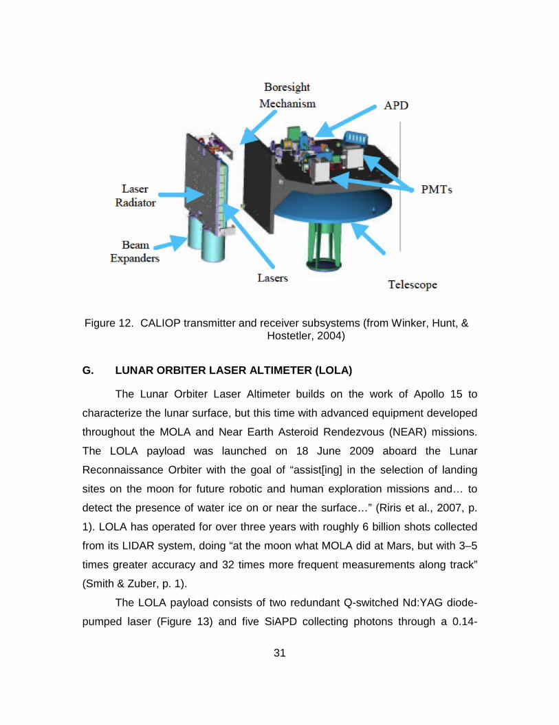
Figure 12. CALIOP transmitter and receiver subsystems (from Winker, Hunt, &
Hostetler, 2004)
G. LUNAR ORBITER LASER ALTIMETER (LOLA)
The Lunar Orbiter Laser Altimeter builds on the work of Apollo 15 to
characterize the lunar surface, but this time with advanced equipment developed
throughout the MOLA and Near Earth Asteroid Rendezvous (NEAR) missions.
The LOLA payload was launched on 18 June 2009 aboard the Lunar
Reconnaissance Orbiter with the goal of “assist[ing] in the selection of landing
sites on the moon for future robotic and human exploration missions and… to
detect the presence of water ice on or near the surface…” (Riris et al., 2007, p.
1). LOLA has operated for over three years with roughly 6 billion shots collected
from its LIDAR system, doing “at the moon what MOLA did at Mars, but with 3–5
times greater accuracy and 32 times more frequent measurements along track”
(Smith & Zuber, p. 1).
The LOLA payload consists of two redundant Q-switched Nd:YAG diode-
pumped laser (Figure 13) and five SiAPD collecting photons through a 0.14-
31
meter aperture. In a 40-km circular orbit, the 9.6-kg, 26.2-W payload collects data
with a 10 to 15-meter post spacing and 30-cm vertical accuracy. The LOLA
payload differs from the MOLA payload due to its use of the first diffractive optical
element (DOE) to split a single beam into five separate beams. The DOE follows
a diode-pumped Nd:YAG amplifier operating at 28 Hz with a 5-nanosecond
pulse-width providing 3.2 mJ per pulse. The receiver follows the design of that
flown on MOLA but consists of five SiAPDs fiber-coupled to the receive optics to
provide a 20-meter IFOV while the laser illuminates a 5-meter target within each
IFOV (Riris & Cavanaugh, 2010). LOLA remains relatively inefficient compared to
current technology but due to the new design and the near-zero lunar
atmosphere, improvements in post-spacing and reliability were realized,
successfully implemented and enable operation to this day.
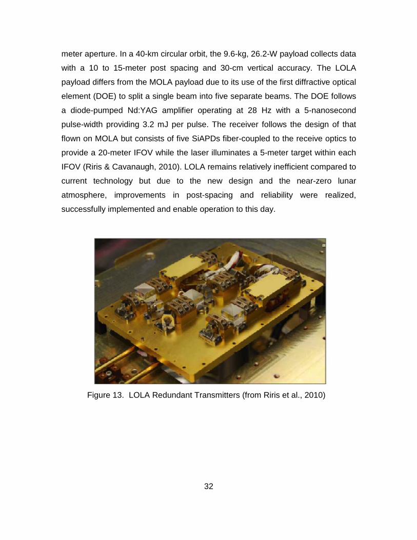
Figure 13. LOLA Redundant Transmitters (from Riris et al., 2010)
32
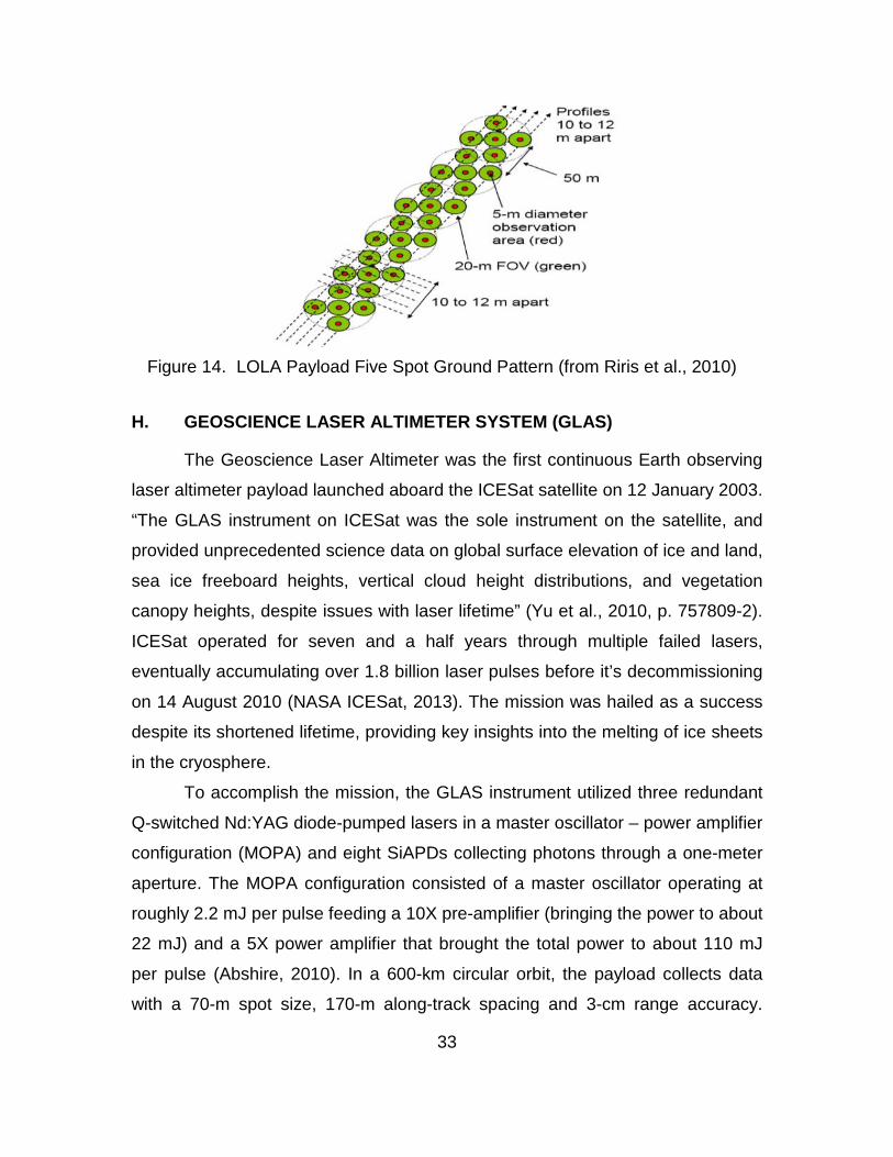
Figure 14. LOLA Payload Five Spot Ground Pattern (from Riris et al., 2010)
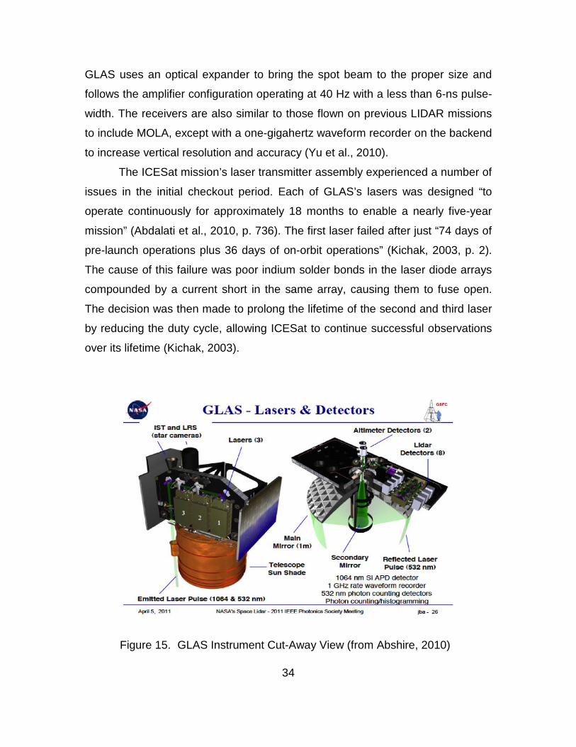
H. GEOSCIENCE LASER ALTIMETER SYSTEM (GLAS)
The Geoscience Laser Altimeter was the first continuous Earth observing
laser altimeter payload launched aboard the ICESat satellite on 12 January 2003.
“The GLAS instrument on ICESat was the sole instrument on the satellite, and
provided unprecedented science data on global surface elevation of ice and land,
sea ice freeboard heights, vertical cloud height distributions, and vegetation
canopy heights, despite issues with laser lifetime” (Yu et al., 2010, p. 757809-2).
ICESat operated for seven and a half years through multiple failed lasers,
eventually accumulating over 1.8 billion laser pulses before it’s decommissioning
on 14 August 2010 (NASA ICESat, 2013). The mission was hailed as a success
despite its shortened lifetime, providing key insights into the melting of ice sheets
in the cryosphere.
To accomplish the mission, the GLAS instrument utilized three redundant
Q-switched Nd:YAG diode-pumped lasers in a master oscillator – power amplifier
configuration (MOPA) and eight SiAPDs collecting photons through a one-meter
aperture. The MOPA configuration consisted of a master oscillator operating at
roughly 2.2 mJ per pulse feeding a 10X pre-amplifier (bringing the power to about
22 mJ) and a 5X power amplifier that brought the total power to about 110 mJ
per pulse (Abshire, 2010). In a 600-km circular orbit, the payload collects data
with a 70-m spot size, 170-m along-track spacing and 3-cm range accuracy.
33
GLAS uses an optical expander to bring the spot beam to the proper size and
follows the amplifier configuration operating at 40 Hz with a less than 6-ns pulse-
width. The receivers are also similar to those flown on previous LIDAR missions
to include MOLA, except with a one-gigahertz waveform recorder on the backend
to increase vertical resolution and accuracy (Yu et al., 2010).
The ICESat mission’s laser transmitter assembly experienced a number of
issues in the initial checkout period. Each of GLAS’s lasers was designed “to
operate continuously for approximately 18 months to enable a nearly five-year
mission” (Abdalati et al., 2010, p. 736). The first laser failed after just “74 days of
pre-launch operations plus 36 days of on-orbit operations” (Kichak, 2003, p. 2).
The cause of this failure was poor indium solder bonds in the laser diode arrays
compounded by a current short in the same array, causing them to fuse open.
The decision was then made to prolong the lifetime of the second and third laser
by reducing the duty cycle, allowing ICESat to continue successful observations
over its lifetime (Kichak, 2003).
Figure 15. GLAS Instrument Cut-Away View (from Abshire, 2010)
34
I. ICESAT-2
NASA’s ICESat-2 mission, slated for launch in July 2016, is the follow-on
to ICESat-1 and will carry the ATLAS payload. The payload and space vehicle for
ICESat-2 are in the Phase C or “Design and Development” stage according to
NASA’s ICESat-2 website, with technologies and conceptual designs selected for
flight (NASA: ICESat-2, 2013). The mission of ICESat-2 will be similar in scope to
ICESat-1’s, which prematurely ended in 2010 due to laser transmitter anomalies.
In particular, ICESat-2 will measure the temporal and spatial character of ice sheet elevation change to enable assessment of ice sheet mass balance and examination of the underlying mechanisms that control it. The precision of ICESat-2’s elevation measurement will also allow for accurate measurements of sea ice freeboard height, from which sea ice thickness and its temporal changes can be estimated. ICESat-2 will provide important information on other components of the Earth System as well, most notably large-scale vegetation biomass estimates through the measurement of vegetation canopy height. When combined with the original ICESat observations, ICESat-2 will provide ice change measurements across more than a 15-year time span. Its significantly improved laser system will also provide observations with much greater spatial resolution, temporal resolution, and accuracy than has ever been possible before. (Abdalati et al., 2010, p. 735)
To accomplish this mission, Advanced Topographic Laser Altimeter
System (ATLAS) will depart from many of the historical planetary LIDARs
including ICESat-1’s GLAS design, which primarily used an analog detection
scheme and 1064 nm lasers (although ICESat-1 did have a secondary laser and
detectors at 532 nm). Instead, ATLAS will employ single-photon sensitive
receivers operating with much higher gain and a laser transmitter operating at
532nm, similar to GLAS’s secondary system. The full laser and receiver designs
have yet to be completed at this time, but NASA’s “snapshot” documents offer a
preview of the instrument. ATLAS’s transmitter is a frequency doubled Nd:YVO4
Q-switched MOPA laser. The 1064-nm light is then passed through a second
harmonic generator, in this case a lithium triborate crystal, to generate the
frequency-doubled 532-nm beam with a laser wall-plug efficiency of greater than 35
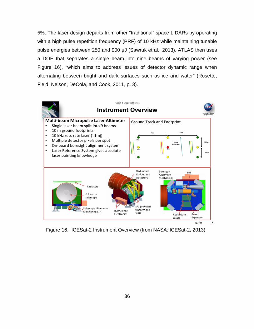
5%. The laser design departs from other “traditional” space LIDARs by operating
with a high pulse repetition frequency (PRF) of 10 kHz while maintaining tunable
pulse energies between 250 and 900 μJ (Sawruk et al., 2013). ATLAS then uses
a DOE that separates a single beam into nine beams of varying power (see
Figure 16), “which aims to address issues of detector dynamic range when
alternating between bright and dark surfaces such as ice and water” (Rosette,
Field, Nelson, DeCola, and Cook, 2011, p. 3).
Figure 16. ICESat-2 Instrument Overview (from NASA: ICESat-2, 2013)
36
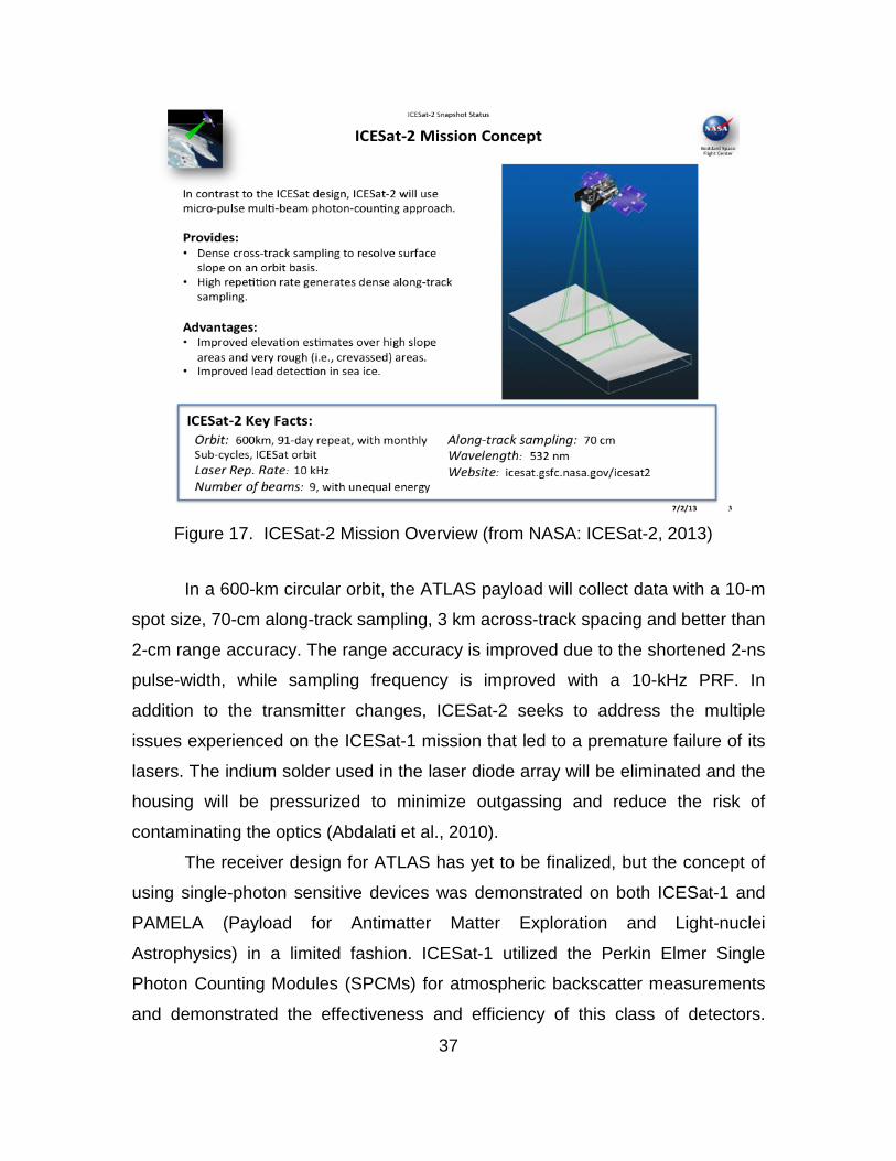
Figure 17. ICESat-2 Mission Overview (from NASA: ICESat-2, 2013)
In a 600-km circular orbit, the ATLAS payload will collect data with a 10-m
spot size, 70-cm along-track sampling, 3 km across-track spacing and better than
2-cm range accuracy. The range accuracy is improved due to the shortened 2-ns
pulse-width, while sampling frequency is improved with a 10-kHz PRF. In
addition to the transmitter changes, ICESat-2 seeks to address the multiple
issues experienced on the ICESat-1 mission that led to a premature failure of its
lasers. The indium solder used in the laser diode array will be eliminated and the
housing will be pressurized to minimize outgassing and reduce the risk of
contaminating the optics (Abdalati et al., 2010).
The receiver design for ATLAS has yet to be finalized, but the concept of
using single-photon sensitive devices was demonstrated on both ICESat-1 and
PAMELA (Payload for Antimatter Matter Exploration and Light-nuclei
Astrophysics) in a limited fashion. ICESat-1 utilized the Perkin Elmer Single
Photon Counting Modules (SPCMs) for atmospheric backscatter measurements
and demonstrated the effectiveness and efficiency of this class of detectors.
37
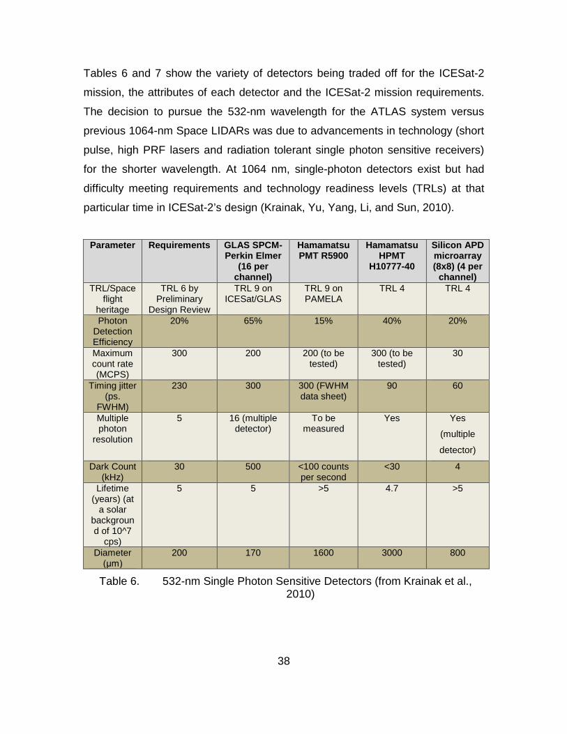
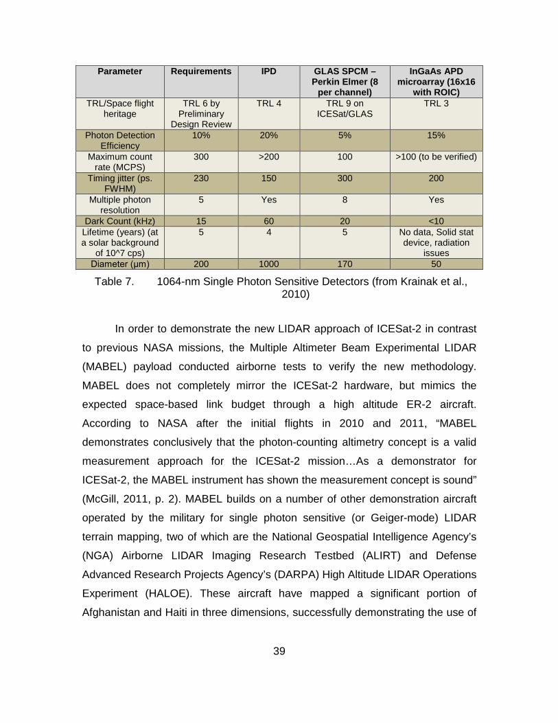
Tables 6 and 7 show the variety of detectors being traded off for the ICESat-2
mission, the attributes of each detector and the ICESat-2 mission requirements.
The decision to pursue the 532-nm wavelength for the ATLAS system versus
previous 1064-nm Space LIDARs was due to advancements in technology (short
pulse, high PRF lasers and radiation tolerant single photon sensitive receivers)
for the shorter wavelength. At 1064 nm, single-photon detectors exist but had
difficulty meeting requirements and technology readiness levels (TRLs) at that
particular time in ICESat-2’s design (Krainak, Yu, Yang, Li, and Sun, 2010).
Parameter Requirements GLAS SPCM-
Perkin Elmer (16 per
channel)
Hamamatsu PMT R5900
Hamamatsu HPMT
H10777-40
Silicon APD microarray (8x8) (4 per
channel) TRL/Space
flight heritage
TRL 6 by Preliminary
Design Review
TRL 9 on ICESat/GLAS
TRL 9 on PAMELA
TRL 4 TRL 4
Photon Detection Efficiency
20% 65% 15% 40% 20%
Maximum count rate (MCPS)
300 200 200 (to be tested)
300 (to be tested)
30
Timing jitter (ps.
FWHM)
230 300 300 (FWHM data sheet)
90 60
Multiple photon
resolution
5 16 (multiple detector)
To be measured
Yes Yes
(multiple
detector)
Dark Count (kHz)
30 500 <100 counts per second
<30 4
Lifetime (years) (at
a solar background of 10^7
cps)
5 5 >5 4.7 >5
Diameter (μm)
200 170 1600 3000 800
Table 6. 532-nm Single Photon Sensitive Detectors (from Krainak et al., 2010)
38
Parameter Requirements IPD GLAS SPCM –Perkin Elmer (8
per channel)
InGaAs APD microarray (16x16
with ROIC) TRL/Space flight
heritage TRL 6 by
Preliminary Design Review
TRL 4 TRL 9 on ICESat/GLAS
TRL 3
Photon Detection Efficiency
10% 20% 5% 15%
Maximum count rate (MCPS)
300 >200 100 >100 (to be verified)
Timing jitter (ps. FWHM)
230 150 300 200
Multiple photon resolution
5 Yes 8 Yes
Dark Count (kHz) 15 60 20 <10 Lifetime (years) (at a solar background
of 10^7 cps)
5 4 5 No data, Solid stat device, radiation
issues Diameter (μm) 200 1000 170 50
Table 7. 1064-nm Single Photon Sensitive Detectors (from Krainak et al., 2010)
In order to demonstrate the new LIDAR approach of ICESat-2 in contrast
to previous NASA missions, the Multiple Altimeter Beam Experimental LIDAR
(MABEL) payload conducted airborne tests to verify the new methodology.
MABEL does not completely mirror the ICESat-2 hardware, but mimics the
expected space-based link budget through a high altitude ER-2 aircraft.
According to NASA after the initial flights in 2010 and 2011, “MABEL
demonstrates conclusively that the photon-counting altimetry concept is a valid
measurement approach for the ICESat-2 mission…As a demonstrator for
ICESat-2, the MABEL instrument has shown the measurement concept is sound”
(McGill, 2011, p. 2). MABEL builds on a number of other demonstration aircraft
operated by the military for single photon sensitive (or Geiger-mode) LIDAR
terrain mapping, two of which are the National Geospatial Intelligence Agency’s
(NGA) Airborne LIDAR Imaging Research Testbed (ALIRT) and Defense
Advanced Research Projects Agency’s (DARPA) High Altitude LIDAR Operations
Experiment (HALOE). These aircraft have mapped a significant portion of
Afghanistan and Haiti in three dimensions, successfully demonstrating the use of
39
single-photon sensitive devices (these two specifically at 1064 nm) even prior to
MABEL’s test flights.
LIDAR has had a long and storied history in space, dating back to the
Apollo missions that helped map the lunar surface in 1971. ICESat-2 is the latest
generation of LIDAR sensors to be designed, having evolved from ruby lasers
and analog receivers to high efficiency fiber lasers and single photon sensitive
arrays. As the technology progresses, the missions continue to push towards
more robust and higher resolution elevation measurements to tackle ever more
challenging requirements.
40
IV. SPACE-BASED LIDAR COST CONSIDERATIONS
NASA’s primary challenge in the next few years will be to complete a series of complex and expensive projects in the context of constrained budgets and sometimes competing priorities set by the Congress and the administration.
–NASA Assessments of Selected Large-Scale Projects, 2013, p. 23
Mission cost remains a key factor in determining the viability of a mission
for government agencies, especially in the face of sequestration and a budget-
constrained environment. Programs with high return-on-investment still require
rigorous cost accounting procedures and independent cost estimates (ICE) to
verify long-term program costs. These independent cost estimates involve
multiple parametric models to calculate overall program costs and potential cost
overruns with a high confidence level. This section does not provide a high
fidelity ICE-like cost profile, but rather a first cut analysis on the main cost drivers
for a space-LIDAR mission and historical cost knowledge.
A. HISTORICAL COSTS AND ICESAT-2 ESTIMATES
NASA has launched a number of space-based LIDAR missions in the past
three decades to map and monitor the Moon, Mercury, and Mars and, with
ICESat-1, Earth. The MESSENGER spacecraft was launched in 2004 and slated
to study “Mercury’s mysterious magnetic field and unusual activity” (Huffington
Post, 2011, p. 1). On-board MESSENGER was a number of instruments with one
of the payloads consisting of a Nd:YAG LIDAR system to map the topography of
Mercury. The 1000-kg spacecraft and payloads continues to operate successfully
for over two years (with a six-year transit time) at a cost of $446M.
The Lunar Reconnaissance Orbiter was launched in 2008 and continues
operations with its LIDAR payload, a Nd:YAG system having cataloged over 1
billion shots. The mission, at a cost of $504M, was “equipped with seven state-of-
the-art cameras and other instruments… [looking] for suitable landing sites for
41
future manned missions while creating the most detailed lunar atlas ever
assembled” (Harwood, 2009, p. 1). The 4,200-lbs spacecraft was launched on an
Atlas V and has successfully mapped the topography of the moon in
unprecedented detail.
While both the MESSENGER and LRO spacecraft demonstrated the utility
and potential costs of a LIDAR system, it was not until 2003 when an Earth-
observing LIDAR was specifically designed and launched into space for
continuous operations. There are significant differences between the Earth
observing mission and the inter-planetary missions due to atmospheric variables,
the need for inter-planetary missions to transit to their location, radiation profiles
and a multitude of other spacecraft differences. The inter-planetary costs provide
a backdrop for both ICESat-1 and ICESat-2’s cost profiles. ICESat-1 actual cost
profiles are difficult to calculate due to the lack of full government cost accounting
during the initial phases of ICESat-1, however, expert knowledge of the program
has allowed for rough estimates of the final program cost. Cost estimates for the
entire ICESat-1 system, excluding operations, total roughly $462M. The cost
breakout of the system includes launch costs at $282M for the Delta II launcher,
$55M for the BCP2000 bus and roughly $125M for the payload (Silverman, 2013;
USA Today, 2003). ICESat-1 followed a similar technology path to previous
missions but ended significantly early in its mission lifetime.
ICESat-2’s initial cost estimate was roughly $650M for the total mission to
include formulation, development, launch and operations. Launch costs are still
uncertain at this point, but the original value of Fibertek’s ATLAS payload and
Orbital’s spacecraft bus and integration contracts were $26M and $135M,
respectively (Leone, 2012). Most recently, the mission cost increased to $860.3M
with a cost breakout of $248.8M for mission formulation, $558M for development
and $52.9M for operations (Government Accountability Office, 2012).
Upon further examination of the limited cost and performance data for
these space vehicles, it is difficult to draw any parallels between payload
performance and spacecraft cost. Due to the limited amount of publically
42
available data and small number of space-borne missions with a LIDAR payload,
any cost trending is inconclusive. Also, the number of variables including
interplanetary versus Earth-observing, multi-payload versus single-payload, and
other environmental conditions make a simple cost trending difficult to determine.
Other non-LIDAR cost models need to be explored to determine a best first-order
fit for a spacecraft cost estimation.
B. SATELLITE COST MODELS
A number of cost estimating methods and models have been developed
over the years to accurately determine a satellite’s cost throughout its
development life-cycle. NASA’s Space Systems Engineering Training’s Cost
Estimation Module describes a number of difficulties and considerations
regarding spacecraft cost estimation. Cost estimation remains a blend of art and
science due to the nature of the models and data that includes: small sample
sizes, incomplete/cloudy historical data, multi-variable cost drivers and unique
one-of-a-kind missions (Guerra, 2008). These challenges do not rule out effective
cost estimation, but only provide a glimpse at the limitations for the aerospace
community.
1. Cost Estimation Methodologies
Three main cost estimation methods exist with varying levels of complexity
and accuracy. Detailed bottom-up estimating is time-consuming and requires
detailed designs and work breakdown structures to calculate total spacecraft
cost. Analogous estimation is based upon similar systems and their associated
costs, but adjusted for differences in size and complexity. This method is fairly
limited due to the inability to perform trade studies within this space. Parametric
cost estimation is the third method available, and can account for a number of
variables and is more easily extensible to trade studies while less time-
consuming than bottom-up estimation. This method relies on historical data and
a number of analogous data points to provide the best possible fit to the data,
while keeping the number of variables manageable (Figure 18). Parametric
43
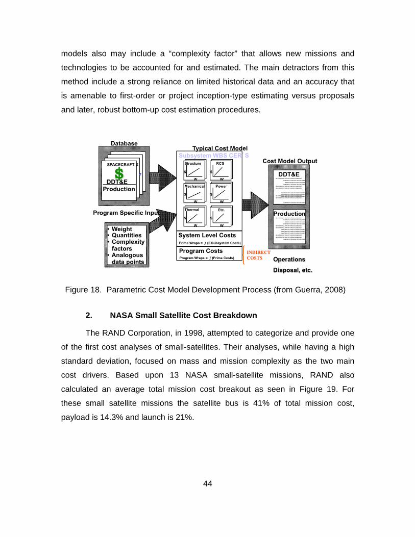
models also may include a “complexity factor” that allows new missions and
technologies to be accounted for and estimated. The main detractors from this
method include a strong reliance on limited historical data and an accuracy that
is amenable to first-order or project inception-type estimating versus proposals
and later, robust bottom-up cost estimation procedures.
Figure 18. Parametric Cost Model Development Process (from Guerra, 2008)
2. NASA Small Satellite Cost Breakdown
The RAND Corporation, in 1998, attempted to categorize and provide one
of the first cost analyses of small-satellites. Their analyses, while having a high
standard deviation, focused on mass and mission complexity as the two main
cost drivers. Based upon 13 NASA small-satellite missions, RAND also
calculated an average total mission cost breakout as seen in Figure 19. For
these small satellite missions the satellite bus is 41% of total mission cost,
payload is 14.3% and launch is 21%.
44
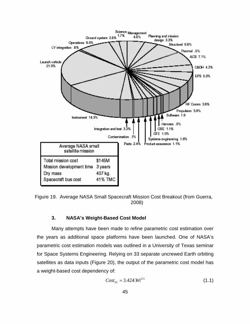
Figure 19. Average NASA Small Spacecraft Mission Cost Breakout (from Guerra,
2008)
3. NASA’s Weight-Based Cost Model
Many attempts have been made to refine parametric cost estimation over
the years as additional space platforms have been launched. One of NASA’s
parametric cost estimation models was outlined in a University of Texas seminar
for Space Systems Engineering. Relying on 33 separate uncrewed Earth orbiting
satellites as data inputs (Figure 20), the output of the parametric cost model has
a weight-based cost dependency of:
0.53.424SCCost Wt= (1.1)
45
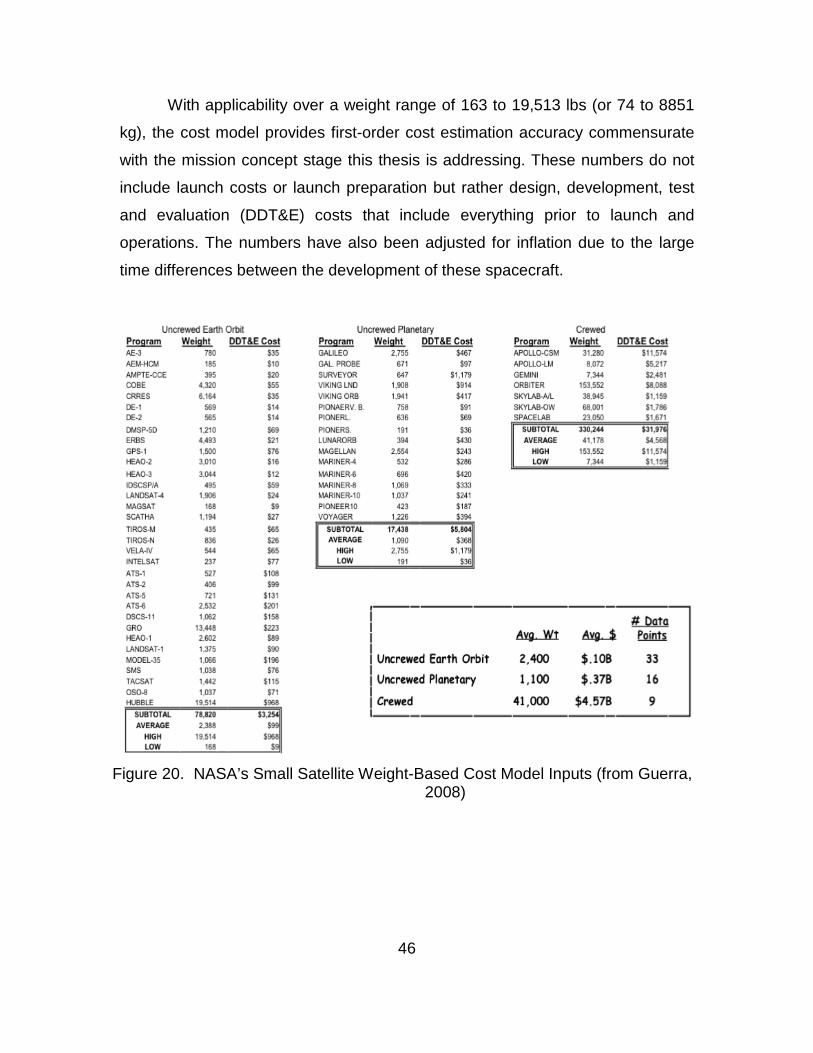
With applicability over a weight range of 163 to 19,513 lbs (or 74 to 8851
kg), the cost model provides first-order cost estimation accuracy commensurate
with the mission concept stage this thesis is addressing. These numbers do not
include launch costs or launch preparation but rather design, development, test
and evaluation (DDT&E) costs that include everything prior to launch and
operations. The numbers have also been adjusted for inflation due to the large
time differences between the development of these spacecraft.
Figure 20. NASA’s Small Satellite Weight-Based Cost Model Inputs (from Guerra,
2008)
46
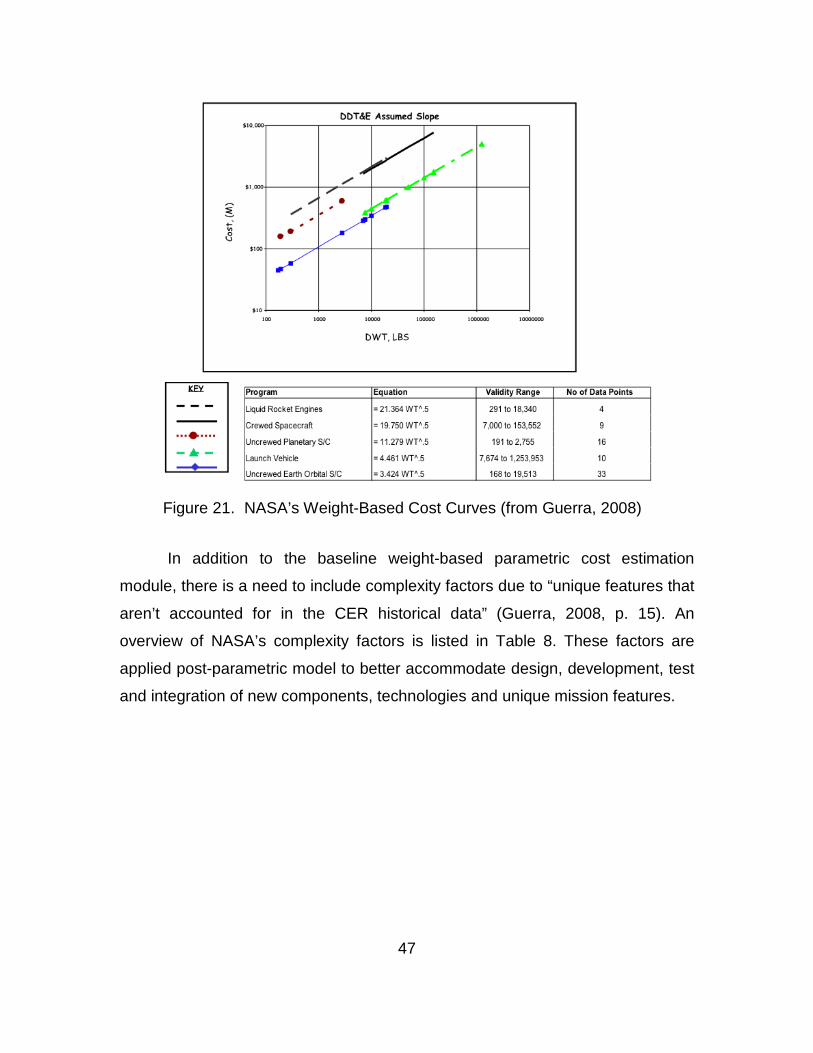
Figure 21. NASA’s Weight-Based Cost Curves (from Guerra, 2008)
In addition to the baseline weight-based parametric cost estimation
module, there is a need to include complexity factors due to “unique features that
aren’t accounted for in the CER historical data” (Guerra, 2008, p. 15). An
overview of NASA’s complexity factors is listed in Table 8. These factors are
applied post-parametric model to better accommodate design, development, test
and integration of new components, technologies and unique mission features.
47
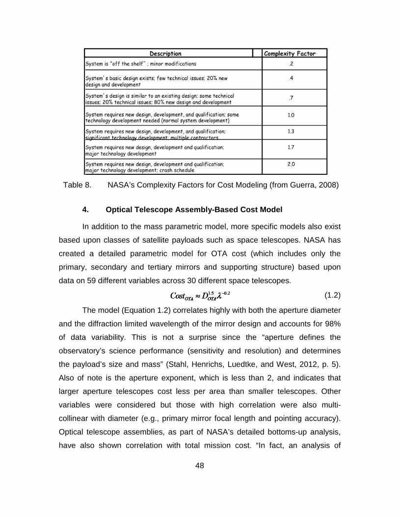
Table 8. NASA’s Complexity Factors for Cost Modeling (from Guerra, 2008)
4. Optical Telescope Assembly-Based Cost Model
In addition to the mass parametric model, more specific models also exist
based upon classes of satellite payloads such as space telescopes. NASA has
created a detailed parametric model for OTA cost (which includes only the
primary, secondary and tertiary mirrors and supporting structure) based upon
data on 59 different variables across 30 different space telescopes.
(1.2)
The model (Equation 1.2) correlates highly with both the aperture diameter
and the diffraction limited wavelength of the mirror design and accounts for 98%
of data variability. This is not a surprise since the “aperture defines the
observatory’s science performance (sensitivity and resolution) and determines
the payload’s size and mass” (Stahl, Henrichs, Luedtke, and West, 2012, p. 5).
Also of note is the aperture exponent, which is less than 2, and indicates that
larger aperture telescopes cost less per area than smaller telescopes. Other
variables were considered but those with high correlation were also multi-
collinear with diameter (e.g., primary mirror focal length and pointing accuracy).
Optical telescope assemblies, as part of NASA’s detailed bottoms-up analysis,
have also shown correlation with total mission cost. “In fact, an analysis of
48

detailed WBS documents for 7 missions shows that the spacecraft accounts for
approximately 34% of the cost, science instruments account for 28%, [and] OTAs
account for 11%” (Stahl et al., 2012, p. 4).
C. STANDARD SPACECRAFT BUSES AND LAUNCH VEHICLES
Spacecraft buses are an integral piece of the cost and operational
limitations of a space-based LIDAR system. While custom buses have been
designed, in order to constrain costs, standard spacecraft buses should be used.
In Tables 9 and 10, current standard buses are identified with their key operating
parameters. These parameters are important as they provide payload constraints
in terms of power, mass, volume, data storage, communication downlink rates,
spacecraft lifetime and pointing.
These spacecraft buses predominantly constrain the size, mass and
power of the payload options. Their size will also help determine the overall mass
of the mission and mass-based cost. For comparison, two previous LIDAR buses
for ICESat-1 and ICESat-2 are described in Table 9 as the BCP-2000 and
LEOStar-3, respectively. The BCP-2000 is a low-cost, lightweight bus that
provides moderate capability and was used on ICESat-1. With strong space
heritage, this bus exceeded on-orbit lifetimes for ICESat-1 but also limits payload
power significantly compared to the LEOStar-3 bus. The LEOStar-3 bus, which is
slated for the ICESat-2 mission, is a larger and more capable bus but comes at
an expense. The ability to provide more power to the payload and increased
pointing accuracy makes this bus attractive for future missions, but its mass is a
concern for future missions. The LEOStar-3 bus has a strong space heritage with
the Landsat 8 and GEOEye-1 missions having flown on-board this bus.
49
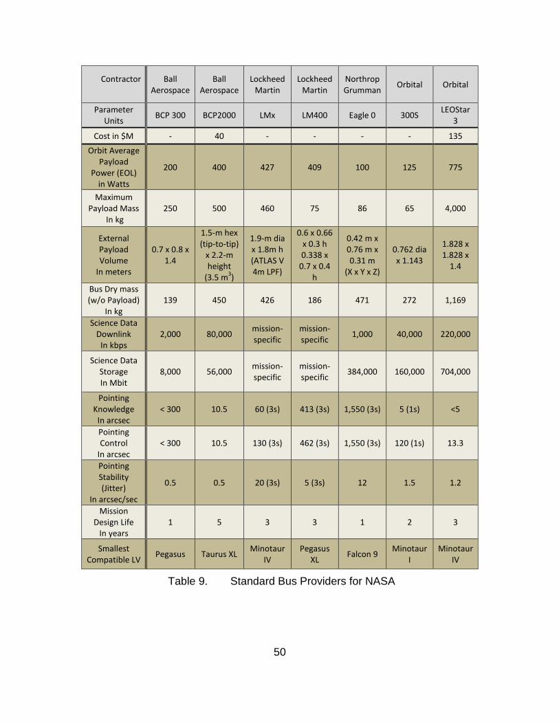
Contractor
Ball Aerospace
Ball Aerospace
Lockheed Martin
Lockheed Martin
Northrop Grumman Orbital Orbital
Parameter Units BCP 300 BCP2000 LMx LM400 Eagle 0 300S LEOStar
3
Cost in $M - 40 - - - - 135
Orbit Average Payload
Power (EOL) in Watts
200 400 427 409 100 125 775
Maximum Payload Mass
In kg 250 500 460 75 86 65 4,000
External Payload Volume
In meters
0.7 x 0.8 x 1.4
1.5-m hex (tip-to-tip)
x 2.2-m height
(3.5 m3)
1.9-m dia x 1.8m h (ATLAS V 4m LPF)
0.6 x 0.66 x 0.3 h 0.338 x
0.7 x 0.4 h
0.42 m x 0.76 m x 0.31 m
(X x Y x Z)
0.762 dia x 1.143
1.828 x 1.828 x
1.4
Bus Dry mass (w/o Payload)
In kg 139 450 426 186 471 272 1,169
Science Data Downlink
In kbps 2,000 80,000 mission-
specific mission-specific 1,000 40,000 220,000
Science Data Storage In Mbit
8,000 56,000 mission-specific
mission-specific 384,000 160,000 704,000
Pointing Knowledge
In arcsec < 300 10.5 60 (3s) 413 (3s) 1,550 (3s) 5 (1s) <5
Pointing Control
In arcsec < 300 10.5 130 (3s) 462 (3s) 1,550 (3s) 120 (1s) 13.3
Pointing Stability (Jitter)
In arcsec/sec
0.5 0.5 20 (3s) 5 (3s) 12 1.5 1.2
Mission Design Life
In years 1 5 3 3 1 2 3
Smallest Compatible LV Pegasus Taurus XL Minotaur
IV Pegasus
XL Falcon 9 Minotaur I
Minotaur IV
Table 9. Standard Bus Providers for NASA
50
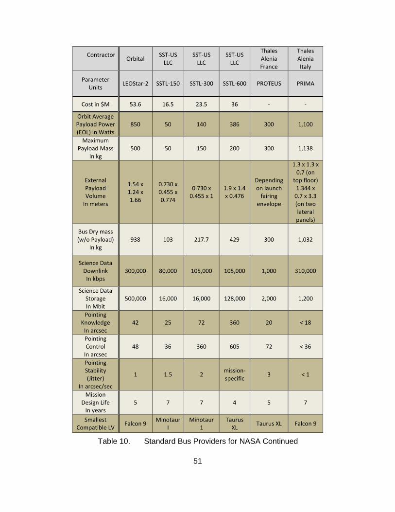
Contractor Orbital SST-US
LLC SST-US
LLC SST-US
LLC
Thales Alenia France
Thales Alenia Italy
Parameter Units LEOStar-2 SSTL-150 SSTL-300 SSTL-600 PROTEUS PRIMA
Cost in $M 53.6 16.5 23.5 36 - -
Orbit Average Payload Power (EOL) in Watts
850 50 140 386 300 1,100
Maximum Payload Mass
In kg 500 50 150 200 300 1,138
External Payload Volume
In meters
1.54 x 1.24 x 1.66
0.730 x 0.455 x 0.774
0.730 x 0.455 x 1
1.9 x 1.4 x 0.476
Depending on launch
fairing envelope
1.3 x 1.3 x 0.7 (on
top floor) 1.344 x
0.7 x 3.3 (on two lateral panels)
Bus Dry mass (w/o Payload)
In kg 938 103 217.7 429 300 1,032
Science Data Downlink
In kbps 300,000 80,000 105,000 105,000 1,000 310,000
Science Data Storage In Mbit
500,000 16,000 16,000 128,000 2,000 1,200
Pointing Knowledge
In arcsec 42 25 72 360 20 < 18
Pointing Control
In arcsec 48 36 360 605 72 < 36
Pointing Stability (Jitter)
In arcsec/sec
1 1.5 2 mission-specific 3 < 1
Mission Design Life
In years 5 7 7 4 5 7
Smallest Compatible LV Falcon 9 Minotaur
I Minotaur
1 Taurus
XL Taurus XL Falcon 9
Table 10. Standard Bus Providers for NASA Continued
51
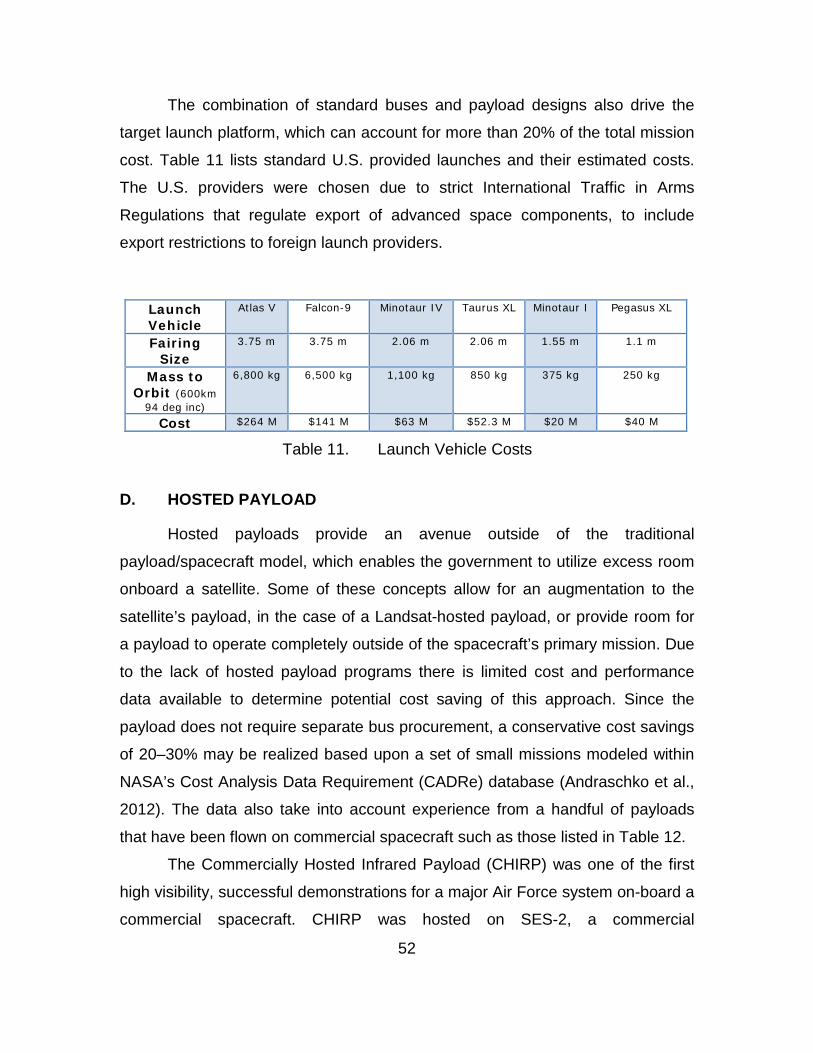
The combination of standard buses and payload designs also drive the
target launch platform, which can account for more than 20% of the total mission
cost. Table 11 lists standard U.S. provided launches and their estimated costs.
The U.S. providers were chosen due to strict International Traffic in Arms
Regulations that regulate export of advanced space components, to include
export restrictions to foreign launch providers.
Table 11. Launch Vehicle Costs
D. HOSTED PAYLOAD
Hosted payloads provide an avenue outside of the traditional
payload/spacecraft model, which enables the government to utilize excess room
onboard a satellite. Some of these concepts allow for an augmentation to the
satellite’s payload, in the case of a Landsat-hosted payload, or provide room for
a payload to operate completely outside of the spacecraft’s primary mission. Due
to the lack of hosted payload programs there is limited cost and performance
data available to determine potential cost saving of this approach. Since the
payload does not require separate bus procurement, a conservative cost savings
of 20–30% may be realized based upon a set of small missions modeled within
NASA’s Cost Analysis Data Requirement (CADRe) database (Andraschko et al.,
2012). The data also take into account experience from a handful of payloads
that have been flown on commercial spacecraft such as those listed in Table 12.
The Commercially Hosted Infrared Payload (CHIRP) was one of the first
high visibility, successful demonstrations for a major Air Force system on-board a
commercial spacecraft. CHIRP was hosted on SES-2, a commercial
Launch Vehicle
Atlas V Falcon-9 Minotaur IV Taurus XL Minotaur I Pegasus XL
Fairing Size
3.75 m 3.75 m 2.06 m 2.06 m 1.55 m 1.1 m
Mass to Orbit (600km
94 deg inc)
6,800 kg 6,500 kg 1,100 kg 850 kg 375 kg 250 kg
Cost $264 M $141 M $63 M $52.3 M $20 M $40 M
52
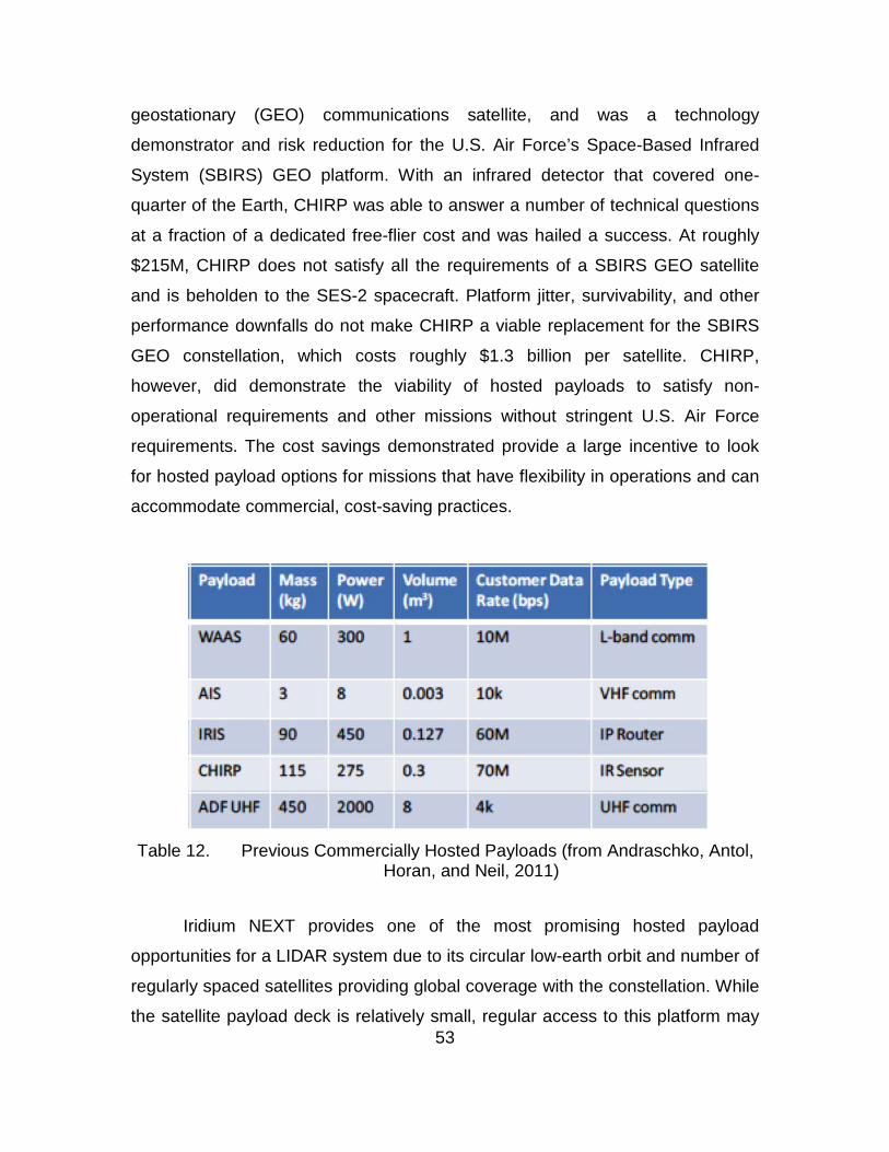
geostationary (GEO) communications satellite, and was a technology
demonstrator and risk reduction for the U.S. Air Force’s Space-Based Infrared
System (SBIRS) GEO platform. With an infrared detector that covered one-
quarter of the Earth, CHIRP was able to answer a number of technical questions
at a fraction of a dedicated free-flier cost and was hailed a success. At roughly
$215M, CHIRP does not satisfy all the requirements of a SBIRS GEO satellite
and is beholden to the SES-2 spacecraft. Platform jitter, survivability, and other
performance downfalls do not make CHIRP a viable replacement for the SBIRS
GEO constellation, which costs roughly $1.3 billion per satellite. CHIRP,
however, did demonstrate the viability of hosted payloads to satisfy non-
operational requirements and other missions without stringent U.S. Air Force
requirements. The cost savings demonstrated provide a large incentive to look
for hosted payload options for missions that have flexibility in operations and can
accommodate commercial, cost-saving practices.
Table 12. Previous Commercially Hosted Payloads (from Andraschko, Antol,
Horan, and Neil, 2011)
Iridium NEXT provides one of the most promising hosted payload
opportunities for a LIDAR system due to its circular low-earth orbit and number of
regularly spaced satellites providing global coverage with the constellation. While
the satellite payload deck is relatively small, regular access to this platform may 53
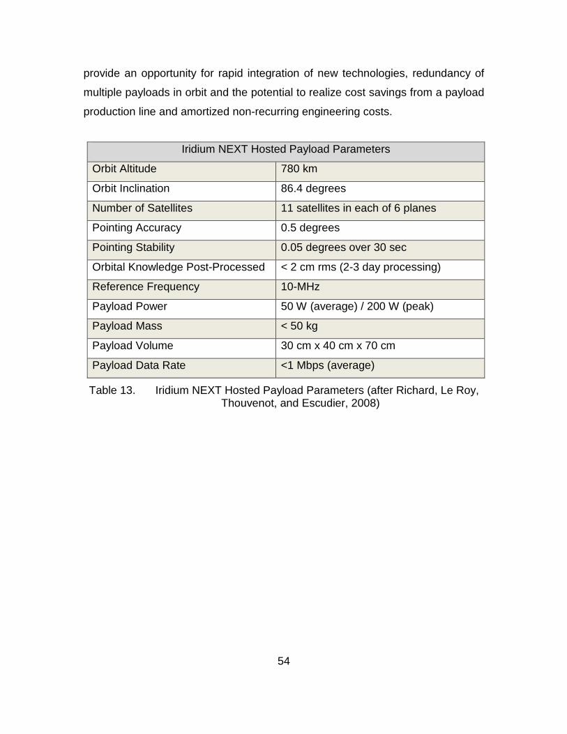
provide an opportunity for rapid integration of new technologies, redundancy of
multiple payloads in orbit and the potential to realize cost savings from a payload
production line and amortized non-recurring engineering costs.
Table 13. Iridium NEXT Hosted Payload Parameters (after Richard, Le Roy, Thouvenot, and Escudier, 2008)
Iridium NEXT Hosted Payload Parameters
Orbit Altitude 780 km
Orbit Inclination 86.4 degrees
Number of Satellites 11 satellites in each of 6 planes
Pointing Accuracy 0.5 degrees
Pointing Stability 0.05 degrees over 30 sec
Orbital Knowledge Post-Processed < 2 cm rms (2-3 day processing)
Reference Frequency 10-MHz
Payload Power 50 W (average) / 200 W (peak)
Payload Mass < 50 kg
Payload Volume 30 cm x 40 cm x 70 cm
Payload Data Rate <1 Mbps (average)
54
V. LIDAR PAYLOAD DESIGN OPTIONS
Space LIDAR payloads are relatively complex instruments that must
survive the rigors of space while maintaining tight tolerances due to the nature of
laser systems and sensitive receivers. Radiation tolerance, efficiencies due to
high power requirements, power handling and system complexity are all key
parameters that affect a space LIDAR design. LIDAR payloads generally consist
of three main subsystems: a laser transmitter, receiver and a beam-
steering/dispersion mechanism. The laser transmitter provides a short pulse of
photons that may either be directed towards the target with its inherent beam
properties or steered/reshaped to accommodate the ground footprint desired (far-
field projection). The receiver then measures the time of flight of the photons to
calculate range values while maintaining signal-to-noise ratios (or dark counts)
that are commensurate with mission goals. The interplay of these devices, their
efficiency and simplicity are necessary to realize a low-cost system for future
space-based LIDARs.
A. TRANSMITTER DESIGN
A number of different materials have been developed as lasing mediums
for a multitude of applications. Solid-state, dye, chemical, metal-vapor,
semiconductor and free-electron lasers are some of the many categories of
lasers available today. Of these, few have been rated for space-use or are
qualified to survive the rigors of launch and on-orbit operations in a minimal-
atmosphere, radiation-rich environment. Solid-state lasers have made up the
bulk of lasers launched into space for remote sensing purposes due to their
relatively small-size, moderate efficiency, limited outgassing and ability to
operate over extended periods of time from electrically-fed, diode sources.
Solid-state lasers, like all laser amplifiers, contain “two elements: a laser
medium in which a population inversion… can be achieved, and a pump process
to supply energy to the system…” (Koechner & Bass, 2003, p. 13). The laser
55
medium for solid-state lasers commonly consist of doped crystalline structures
(e.g., ruby, Nd:YAG, Nd:glass, etc.) that allow photons to build up within the
structure and “lase” at a particular interval. The pump process can utilize any
photon source, but current-day LIDAR systems traditionally use pump diodes to
supply energy to the system. Solid-state lasers that have been flown in space
include ruby and Nd:YAG laser systems that mainly consisted of a switched,
pulse-pumped medium that lased at low-frequencies and efficiencies. MOLA and
MLA both used a single-stage device, which provided 2–3% electrical to photon
conversion efficiencies at 4 and 2 Watts, respectively. These single-stage
devices were replaced by a MOPA configuration in the GLAS payload for
ICESat-1. MOPA configurations achieve higher powers and efficiencies due to
their multi-stage design, using a master oscillator to create a low-power pulse
profile that seeds one or more amplifier stages which are more heavily pumped.
GLAS maintained 3% efficiency at 4W while achieving this at a wavelength
double that of MLA and MOLA. (Coyle, 2005).
1. MOPA Transmitter Overview
The MOPA architecture, despite having experienced difficulties on-board
ICESat-1’s mission, remains the most efficient and highest power solid-state
lasers available and are on-track for ICESat-2’s ATLAS payload. Numerous
trades were made in the ATLAS payload design, which requires short pulse
lengths and high beam quality. The MOPA architecture trades included two high
reliability master oscillator candidates and the three main types of solid-state
power amplifiers, all of which are continuous-wave pumped (Figure 22). These
same trades are relevant for the missions being explored in this paper (Yu et al.,
2010).
56
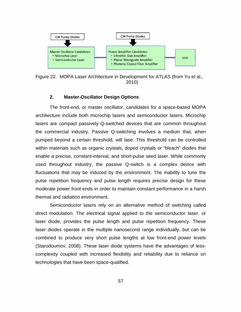
Figure 22. MOPA Laser Architecture in Development for ATLAS (from Yu et al.,
2010)
2. Master-Oscillator Design Options
The front-end, or master oscillator, candidates for a space-based MOPA
architecture include both microchip lasers and semiconductor lasers. Microchip
lasers are compact passively Q-switched devices that are common throughout
the commercial industry. Passive Q-switching involves a medium that, when
pumped beyond a certain threshold, will lase. This threshold can be controlled
within materials such as organic crystals, doped crystals or “bleach” diodes that
enable a precise, constant-interval, and short-pulse seed laser. While commonly
used throughout industry, the passive Q-switch is a complex device with
fluctuations that may be induced by the environment. The inability to tune the
pulse repetition frequency and pulse length requires precise design for these
moderate power front-ends in order to maintain constant performance in a harsh
thermal and radiation environment.
Semiconductor lasers rely on an alternative method of switching called
direct modulation. The electrical signal applied to the semiconductor laser, or
laser diode, provides the pulse length and pulse repetition frequency. These
laser diodes operate in the multiple nanosecond range individually, but can be
combined to produce very short pulse lengths at low front-end power levels
(Starodoumov, 2008). These laser diode systems have the advantages of less-
complexity coupled with increased flexibility and reliability due to reliance on
technologies that have been space-qualified.
57
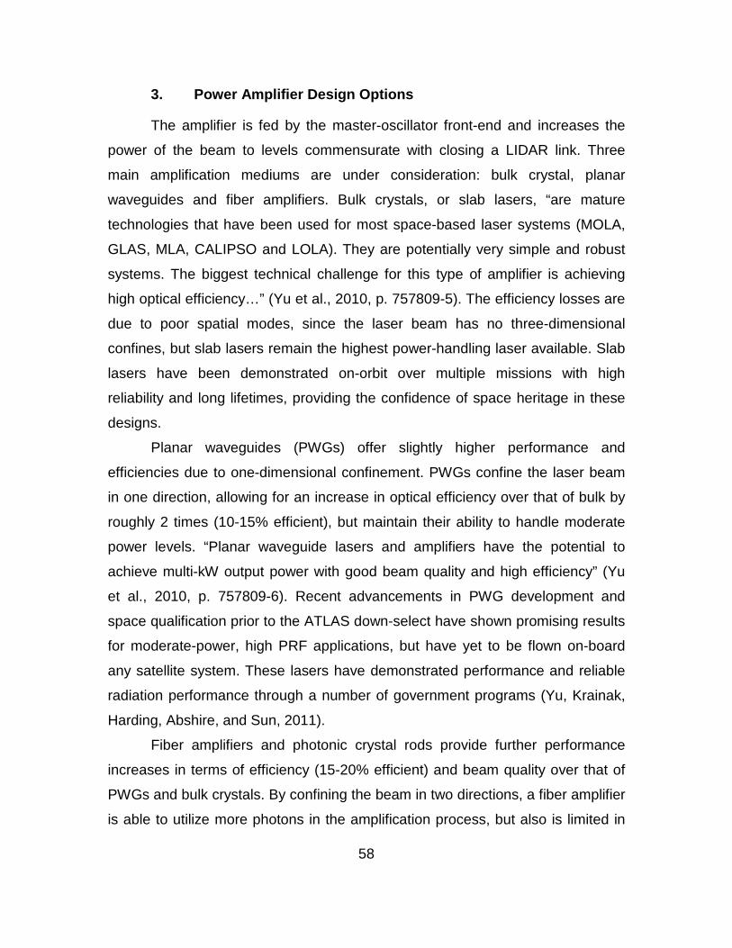
3. Power Amplifier Design Options
The amplifier is fed by the master-oscillator front-end and increases the
power of the beam to levels commensurate with closing a LIDAR link. Three
main amplification mediums are under consideration: bulk crystal, planar
waveguides and fiber amplifiers. Bulk crystals, or slab lasers, “are mature
technologies that have been used for most space-based laser systems (MOLA,
GLAS, MLA, CALIPSO and LOLA). They are potentially very simple and robust
systems. The biggest technical challenge for this type of amplifier is achieving
high optical efficiency…” (Yu et al., 2010, p. 757809-5). The efficiency losses are
due to poor spatial modes, since the laser beam has no three-dimensional
confines, but slab lasers remain the highest power-handling laser available. Slab
lasers have been demonstrated on-orbit over multiple missions with high
reliability and long lifetimes, providing the confidence of space heritage in these
designs.
Planar waveguides (PWGs) offer slightly higher performance and
efficiencies due to one-dimensional confinement. PWGs confine the laser beam
in one direction, allowing for an increase in optical efficiency over that of bulk by
roughly 2 times (10-15% efficient), but maintain their ability to handle moderate
power levels. “Planar waveguide lasers and amplifiers have the potential to
achieve multi-kW output power with good beam quality and high efficiency” (Yu
et al., 2010, p. 757809-6). Recent advancements in PWG development and
space qualification prior to the ATLAS down-select have shown promising results
for moderate-power, high PRF applications, but have yet to be flown on-board
any satellite system. These lasers have demonstrated performance and reliable
radiation performance through a number of government programs (Yu, Krainak,
Harding, Abshire, and Sun, 2011).
Fiber amplifiers and photonic crystal rods provide further performance
increases in terms of efficiency (15-20% efficient) and beam quality over that of
PWGs and bulk crystals. By confining the beam in two directions, a fiber amplifier
is able to utilize more photons in the amplification process, but also is limited in
58
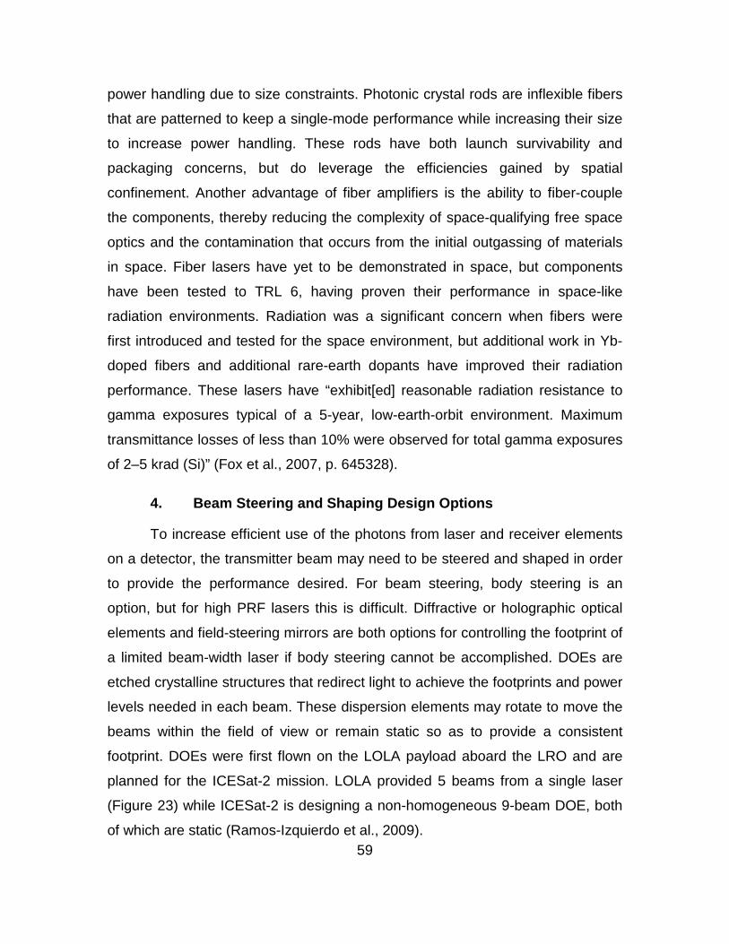
power handling due to size constraints. Photonic crystal rods are inflexible fibers
that are patterned to keep a single-mode performance while increasing their size
to increase power handling. These rods have both launch survivability and
packaging concerns, but do leverage the efficiencies gained by spatial
confinement. Another advantage of fiber amplifiers is the ability to fiber-couple
the components, thereby reducing the complexity of space-qualifying free space
optics and the contamination that occurs from the initial outgassing of materials
in space. Fiber lasers have yet to be demonstrated in space, but components
have been tested to TRL 6, having proven their performance in space-like
radiation environments. Radiation was a significant concern when fibers were
first introduced and tested for the space environment, but additional work in Yb-
doped fibers and additional rare-earth dopants have improved their radiation
performance. These lasers have “exhibit[ed] reasonable radiation resistance to
gamma exposures typical of a 5-year, low-earth-orbit environment. Maximum
transmittance losses of less than 10% were observed for total gamma exposures
of 2–5 krad (Si)” (Fox et al., 2007, p. 645328).
4. Beam Steering and Shaping Design Options
To increase efficient use of the photons from laser and receiver elements
on a detector, the transmitter beam may need to be steered and shaped in order
to provide the performance desired. For beam steering, body steering is an
option, but for high PRF lasers this is difficult. Diffractive or holographic optical
elements and field-steering mirrors are both options for controlling the footprint of
a limited beam-width laser if body steering cannot be accomplished. DOEs are
etched crystalline structures that redirect light to achieve the footprints and power
levels needed in each beam. These dispersion elements may rotate to move the
beams within the field of view or remain static so as to provide a consistent
footprint. DOEs were first flown on the LOLA payload aboard the LRO and are
planned for the ICESat-2 mission. LOLA provided 5 beams from a single laser
(Figure 23) while ICESat-2 is designing a non-homogeneous 9-beam DOE, both
of which are static (Ramos-Izquierdo et al., 2009). 59
Figure 23. LOLA Diffractive Optical Element (from Ramos-Izquierdo et al., 2009)
Field steering mirrors (FSMs) are another option for controlling the beam
footprint. FSMs are commonly used when greater beam control is needed, such
as for sweeping or scanning, and are also aligned with the receive path. Steering
mirrors are actuated structures and “capable of producing three-axis movements
(tip, tilt, and piston)” to provide maximum pointing flexibility (Tapos et al., 2005, p.
587707-1). FSMs, however, add a level of complexity to system design due to
the additional control software and thermal modeling needed. In a zero-gravity
environment, the effects of FSM motion and jitter on the platform must also be
considered, but are well understood with TRL-9, flight-proven products available.
Figure 24. Fast Steering Mirror Exploded View (from Applied Technology
Associates, 2011)
60
Other options exist for beam shaping depending on the transmitter
selection, if any beam-shaping or steering is necessary. For multi-laser systems
(e.g., fiber laser arrays), the pulse power can be apportioned across multiple
transmitters versus a single pumped source. Since LIDAR does not rely on a
coherent, phase-matched signal to make time-of-flight measurements, lasers can
be tiled and incoherently combined in the far-field to produce the footprint
desired. With laser light being highly collimated, divergence can also be
controlled for each footprint with little added system complexity. In some cases,
no beam-shaping or steering may be necessary and only beam divergence will
need to be controlled to determine the optimal footprint.
B. RECEIVER DESIGN
Multiple sensitive, high-efficiency receivers exist to support space-based
LIDAR missions that operate in photon-starved environments. The higher the
efficiency of the detector, the lower the laser power required to obtain the same
area collection rate, driving the need for high sensitivity receivers. NASA, as part
of ICESat-2, recently examined the field of photon-multiplying receivers in both
the visible (552-nm) and near-infrared (1064-nm) bands. Since the initial trades
made by NASA for ICESat-2’s LIDAR detectors by Krainak et al., significant
research has been accomplished in the field of single-photon sensitive devices,
with progress made in avalanche photodiode development.
NASA’s examination of LIDAR detectors included a variety of photon-
sensitive detectors such as: analog photo-multiplier tubes (PMTs), digital
photodiodes and Geiger-mode avalanche photodiodes (GmAPDs). Analog PMTs
have a long history aboard NASA space-based missions, providing robust space-
qualified LIDAR receiver solutions. These detectors utilize dynodes, or photo-
electron multiplication areas, to amplify a signal, but suffer from limited sensitivity
and moderate noise. These detectors required tens to hundreds of photons to
trigger a detection due to the gain and noise shortfalls. Recently, alternative low-
noise single-photon-sensitive detectors have emerged, such as avalanche
photodiodes. 61
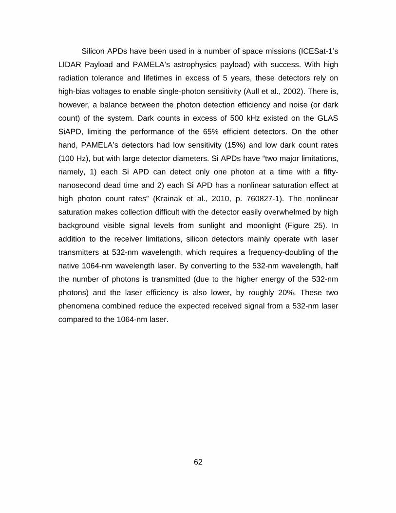
Silicon APDs have been used in a number of space missions (ICESat-1’s
LIDAR Payload and PAMELA’s astrophysics payload) with success. With high
radiation tolerance and lifetimes in excess of 5 years, these detectors rely on
high-bias voltages to enable single-photon sensitivity (Aull et al., 2002). There is,
however, a balance between the photon detection efficiency and noise (or dark
count) of the system. Dark counts in excess of 500 kHz existed on the GLAS
SiAPD, limiting the performance of the 65% efficient detectors. On the other
hand, PAMELA’s detectors had low sensitivity (15%) and low dark count rates
(100 Hz), but with large detector diameters. Si APDs have “two major limitations,
namely, 1) each Si APD can detect only one photon at a time with a fifty-
nanosecond dead time and 2) each Si APD has a nonlinear saturation effect at
high photon count rates” (Krainak et al., 2010, p. 760827-1). The nonlinear
saturation makes collection difficult with the detector easily overwhelmed by high
background visible signal levels from sunlight and moonlight (Figure 25). In
addition to the receiver limitations, silicon detectors mainly operate with laser
transmitters at 532-nm wavelength, which requires a frequency-doubling of the
native 1064-nm wavelength laser. By converting to the 532-nm wavelength, half
the number of photons is transmitted (due to the higher energy of the 532-nm
photons) and the laser efficiency is also lower, by roughly 20%. These two
phenomena combined reduce the expected received signal from a 532-nm laser
compared to the 1064-nm laser.
62
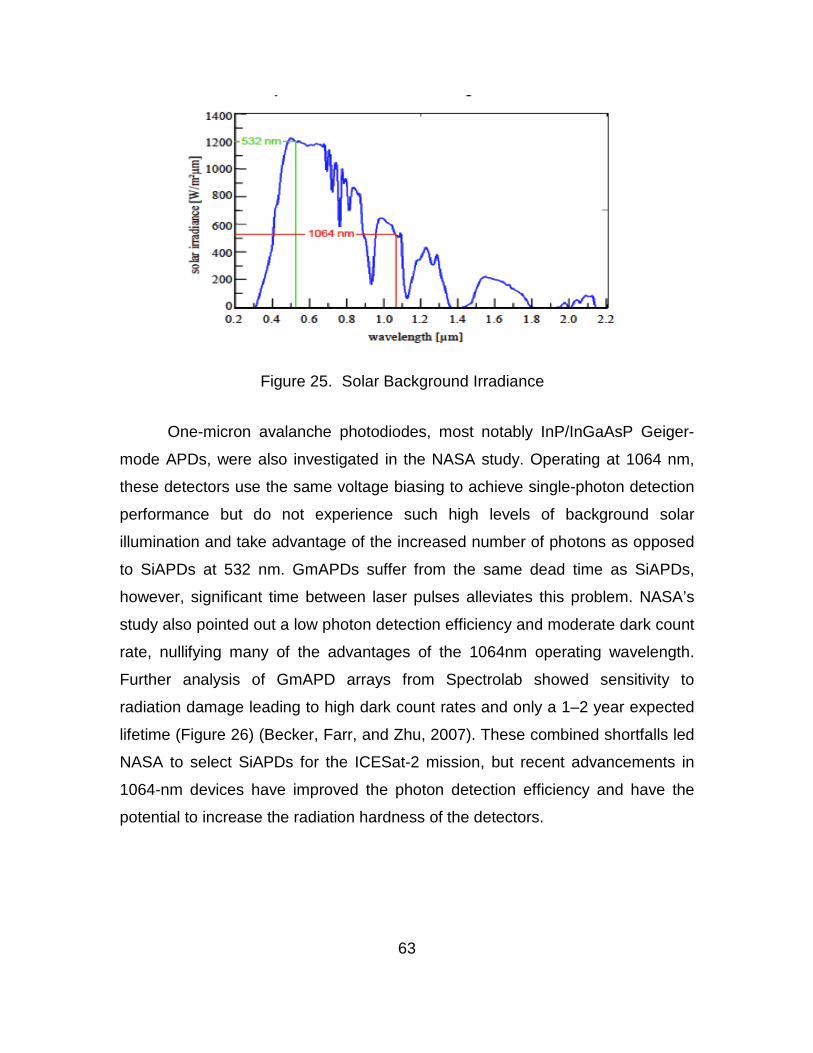
Figure 25. Solar Background Irradiance
One-micron avalanche photodiodes, most notably InP/InGaAsP Geiger-
mode APDs, were also investigated in the NASA study. Operating at 1064 nm,
these detectors use the same voltage biasing to achieve single-photon detection
performance but do not experience such high levels of background solar
illumination and take advantage of the increased number of photons as opposed
to SiAPDs at 532 nm. GmAPDs suffer from the same dead time as SiAPDs,
however, significant time between laser pulses alleviates this problem. NASA’s
study also pointed out a low photon detection efficiency and moderate dark count
rate, nullifying many of the advantages of the 1064nm operating wavelength.
Further analysis of GmAPD arrays from Spectrolab showed sensitivity to
radiation damage leading to high dark count rates and only a 1–2 year expected
lifetime (Figure 26) (Becker, Farr, and Zhu, 2007). These combined shortfalls led
NASA to select SiAPDs for the ICESat-2 mission, but recent advancements in
1064-nm devices have improved the photon detection efficiency and have the
potential to increase the radiation hardness of the detectors.
63
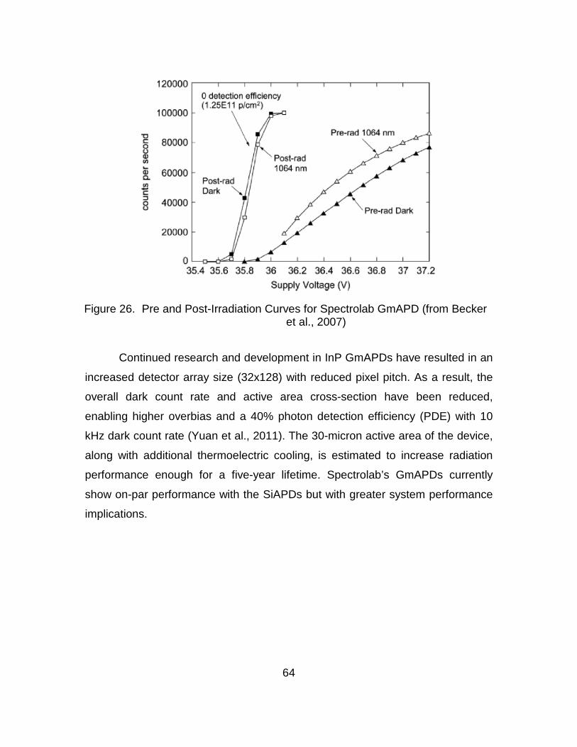
Figure 26. Pre and Post-Irradiation Curves for Spectrolab GmAPD (from Becker
et al., 2007)
Continued research and development in InP GmAPDs have resulted in an
increased detector array size (32x128) with reduced pixel pitch. As a result, the
overall dark count rate and active area cross-section have been reduced,
enabling higher overbias and a 40% photon detection efficiency (PDE) with 10
kHz dark count rate (Yuan et al., 2011). The 30-micron active area of the device,
along with additional thermoelectric cooling, is estimated to increase radiation
performance enough for a five-year lifetime. Spectrolab’s GmAPDs currently
show on-par performance with the SiAPDs but with greater system performance
implications.
64
VI. LIDAR MISSION DESIGN
A. LINK BUDGET
There are a number of effects and physical processes that factor into the
link budget for a space-based LIDAR system. Atmospheric absorption, Mie and
Rayleigh scattering, atmospheric refraction and target surface reflectance
characteristics are key environmental parameters in link budget calculations.
Figure 27 illustrates a number of the variables that affect a space-based LIDAR
system. In the transmission path, the atmosphere attenuates (or absorbs) part of
the transmitted power due to water and aerosol absorption and scattering. This
attenuation is wavelength dependent. The atmosphere also will refract the
transmitted beam due to differences in atmospheric density. Atmospheric
refraction is the bending of light through the atmosphere that causes both beam
spreading and a transmitter/receiver spatial offset that also can be modeled and
is assumed to be negligible in the design of this direct detect system. Also in the
transmission path is additional beam-spreading caused by atmospheric
turbulence and the transmit optics. This will ultimately determine the footprint of
the laser on the ground. In addition to the atmospheric effects, jitter, drift and
broadening of the laser pulse may occur and need to be compensated in the
system. These effects may originate from thermal variations in the laser
components as well as spacecraft structural warping from temperature
differences.
In the receive path, the footprint must be aligned with the receiver footprint
to maximize photons received. Footprint overlap may vary due to thermal
variations in the transmitter and receiver as well as lead-lag considerations due
to the high altitude and speed of the spacecraft. The lead-lag considerations
require approximate terrain knowledge to understand the time of flight for a
photon and the spacecraft pointing compensation required since it is moving at
such a high rate of speed. Also in the receive path are the major effects of
topographical scatter and multi-bounce. The laser will scatter off the surface of
65
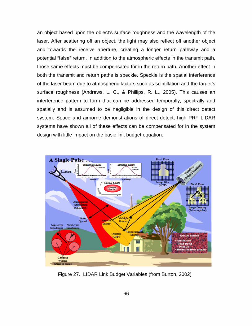
an object based upon the object’s surface roughness and the wavelength of the
laser. After scattering off an object, the light may also reflect off another object
and towards the receive aperture, creating a longer return pathway and a
potential “false” return. In addition to the atmospheric effects in the transmit path,
those same effects must be compensated for in the return path. Another effect in
both the transmit and return paths is speckle. Speckle is the spatial interference
of the laser beam due to atmospheric factors such as scintillation and the target’s
surface roughness (Andrews, L. C., & Phillips, R. L., 2005). This causes an
interference pattern to form that can be addressed temporally, spectrally and
spatially and is assumed to be negligible in the design of this direct detect
system. Space and airborne demonstrations of direct detect, high PRF LIDAR
systems have shown all of these effects can be compensated for in the system
design with little impact on the basic link budget equation.
Figure 27. LIDAR Link Budget Variables (from Burton, 2002)
66
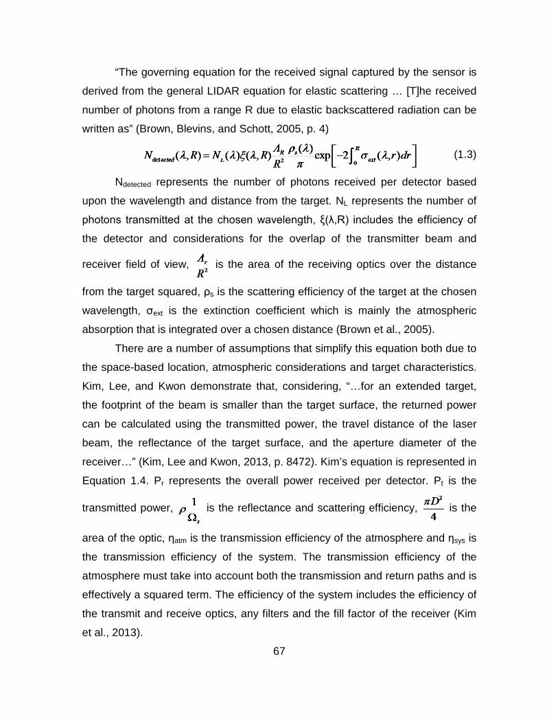
“The governing equation for the received signal captured by the sensor is
derived from the general LIDAR equation for elastic scattering … [T]he received
number of photons from a range R due to elastic backscattered radiation can be
written as” (Brown, Blevins, and Schott, 2005, p. 4)
(1.3)
Ndetected represents the number of photons received per detector based
upon the wavelength and distance from the target. NL represents the number of
photons transmitted at the chosen wavelength, ξ(λ,R) includes the efficiency of
the detector and considerations for the overlap of the transmitter beam and
receiver field of view, is the area of the receiving optics over the distance
from the target squared, ρs is the scattering efficiency of the target at the chosen
wavelength, σext is the extinction coefficient which is mainly the atmospheric
absorption that is integrated over a chosen distance (Brown et al., 2005).
There are a number of assumptions that simplify this equation both due to
the space-based location, atmospheric considerations and target characteristics.
Kim, Lee, and Kwon demonstrate that, considering, “…for an extended target,
the footprint of the beam is smaller than the target surface, the returned power
can be calculated using the transmitted power, the travel distance of the laser
beam, the reflectance of the target surface, and the aperture diameter of the
receiver…” (Kim, Lee and Kwon, 2013, p. 8472). Kim’s equation is represented in
Equation 1.4. Pr represents the overall power received per detector. Pt is the
transmitted power, is the reflectance and scattering efficiency, is the
area of the optic, ηatm is the transmission efficiency of the atmosphere and ηsys is
the transmission efficiency of the system. The transmission efficiency of the
atmosphere must take into account both the transmission and return paths and is
effectively a squared term. The efficiency of the system includes the efficiency of
the transmit and receive optics, any filters and the fill factor of the receiver (Kim
et al., 2013).
67
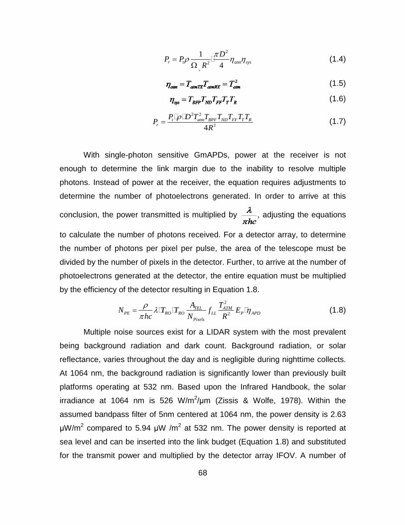
2
2
14
s
r t atm sysDP P
Rπρ η η=
Ω (1.4)
(1.5)
(1.6)
2 2
24t atm BPF ND FF T R
rP D T T T T T TP
Rρ
= (1.7)
With single-photon sensitive GmAPDs, power at the receiver is not
enough to determine the link margin due to the inability to resolve multiple
photons. Instead of power at the receiver, the equation requires adjustments to
determine the number of photoelectrons generated. In order to arrive at this
conclusion, the power transmitted is multiplied by , adjusting the equations
to calculate the number of photons received. For a detector array, to determine
the number of photons per pixel per pulse, the area of the telescope must be
divided by the number of pixels in the detector. Further, to arrive at the number of
photoelectrons generated at the detector, the entire equation must be multiplied
by the efficiency of the detector resulting in Equation 1.8.
2
2TEL ATM
PE RO RO LL P APDPixels
A TN T T f Ehc N Rρ λ η
π= (1.8)
Multiple noise sources exist for a LIDAR system with the most prevalent
being background radiation and dark count. Background radiation, or solar
reflectance, varies throughout the day and is negligible during nighttime collects.
At 1064 nm, the background radiation is significantly lower than previously built
platforms operating at 532 nm. Based upon the Infrared Handbook, the solar
irradiance at 1064 nm is 526 W/m2/μm (Zissis & Wolfe, 1978). Within the
assumed bandpass filter of 5nm centered at 1064 nm, the power density is 2.63
μW/m2 compared to 5.94 μW /m2 at 532 nm. The power density is reported at
sea level and can be inserted into the link budget (Equation 1.8) and substituted
for the transmit power and multiplied by the detector array IFOV. A number of
68
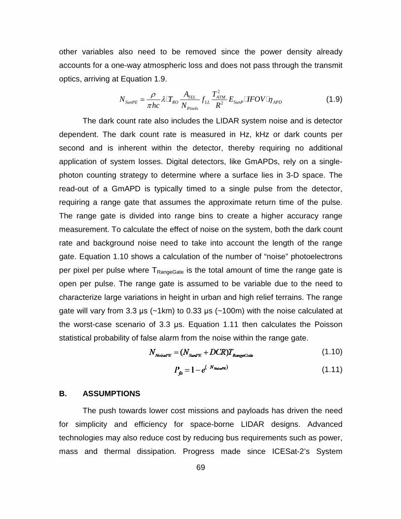
other variables also need to be removed since the power density already
accounts for a one-way atmospheric loss and does not pass through the transmit
optics, arriving at Equation 1.9.
2
2TEL ATM
SunPE RO LL SunP APDPixels
A TN T f E IFOVhc N Rρ λ η
π= (1.9)
The dark count rate also includes the LIDAR system noise and is detector
dependent. The dark count rate is measured in Hz, kHz or dark counts per
second and is inherent within the detector, thereby requiring no additional
application of system losses. Digital detectors, like GmAPDs, rely on a single-
photon counting strategy to determine where a surface lies in 3-D space. The
read-out of a GmAPD is typically timed to a single pulse from the detector,
requiring a range gate that assumes the approximate return time of the pulse.
The range gate is divided into range bins to create a higher accuracy range
measurement. To calculate the effect of noise on the system, both the dark count
rate and background noise need to take into account the length of the range
gate. Equation 1.10 shows a calculation of the number of “noise” photoelectrons
per pixel per pulse where TRangeGate is the total amount of time the range gate is
open per pulse. The range gate is assumed to be variable due to the need to
characterize large variations in height in urban and high relief terrains. The range
gate will vary from 3.3 μs (~1km) to 0.33 μs (~100m) with the noise calculated at
the worst-case scenario of 3.3 μs. Equation 1.11 then calculates the Poisson
statistical probability of false alarm from the noise within the range gate.
(1.10)
(1.11)
B. ASSUMPTIONS
The push towards lower cost missions and payloads has driven the need
for simplicity and efficiency for space-borne LIDAR designs. Advanced
technologies may also reduce cost by reducing bus requirements such as power,
mass and thermal dissipation. Progress made since ICESat-2’s System
69
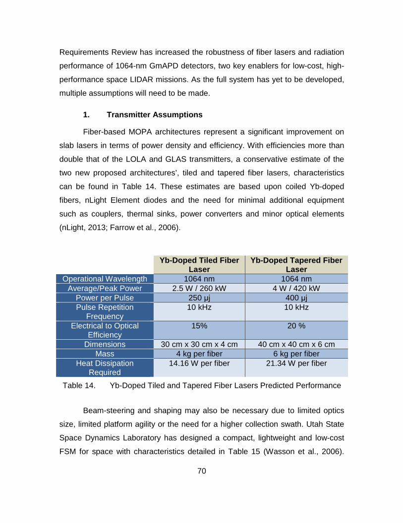
Requirements Review has increased the robustness of fiber lasers and radiation
performance of 1064-nm GmAPD detectors, two key enablers for low-cost, high-
performance space LIDAR missions. As the full system has yet to be developed,
multiple assumptions will need to be made.
1. Transmitter Assumptions
Fiber-based MOPA architectures represent a significant improvement on
slab lasers in terms of power density and efficiency. With efficiencies more than
double that of the LOLA and GLAS transmitters, a conservative estimate of the
two new proposed architectures’, tiled and tapered fiber lasers, characteristics
can be found in Table 14. These estimates are based upon coiled Yb-doped
fibers, nLight Element diodes and the need for minimal additional equipment
such as couplers, thermal sinks, power converters and minor optical elements
(nLight, 2013; Farrow et al., 2006).
Table 14. Yb-Doped Tiled and Tapered Fiber Lasers Predicted Performance
Beam-steering and shaping may also be necessary due to limited optics
size, limited platform agility or the need for a higher collection swath. Utah State
Space Dynamics Laboratory has designed a compact, lightweight and low-cost
FSM for space with characteristics detailed in Table 15 (Wasson et al., 2006).
Yb-Doped Tiled Fiber Laser
Yb-Doped Tapered Fiber Laser
Operational Wavelength 1064 nm 1064 nm Average/Peak Power 2.5 W / 260 kW 4 W / 420 kW
Power per Pulse 250 μj 400 μj Pulse Repetition
Frequency 10 kHz 10 kHz
Electrical to Optical Efficiency
15% 20 %
Dimensions 30 cm x 30 cm x 4 cm 40 cm x 40 cm x 6 cm Mass 4 kg per fiber 6 kg per fiber
Heat Dissipation Required
14.16 W per fiber 21.34 W per fiber
70
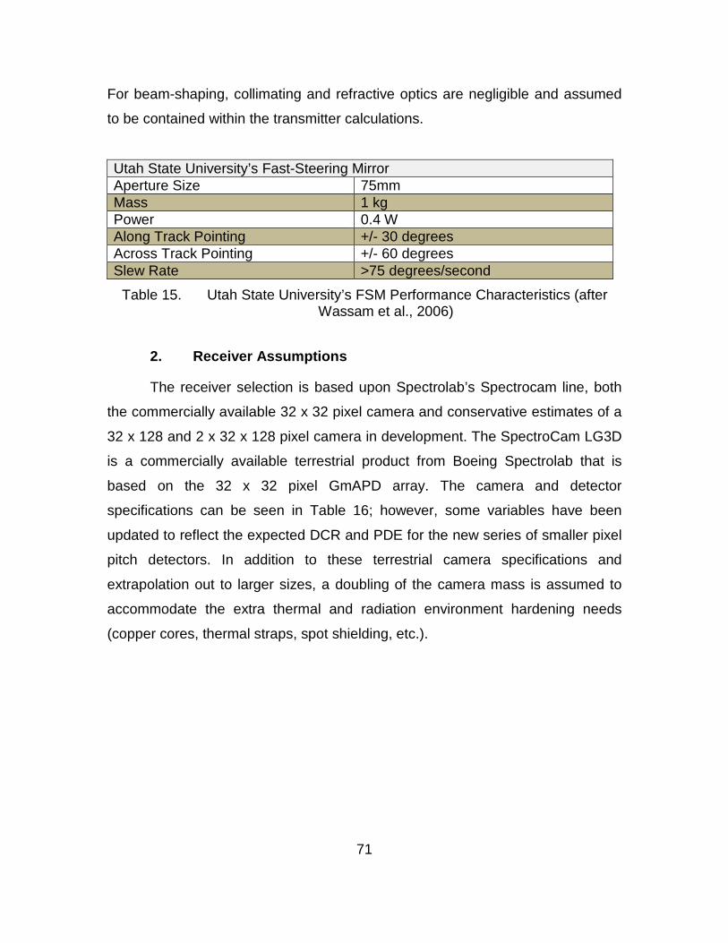
For beam-shaping, collimating and refractive optics are negligible and assumed
to be contained within the transmitter calculations.
Utah State University’s Fast-Steering Mirror Aperture Size 75mm Mass 1 kg Power 0.4 W Along Track Pointing +/- 30 degrees Across Track Pointing +/- 60 degrees Slew Rate >75 degrees/second
Table 15. Utah State University’s FSM Performance Characteristics (after Wassam et al., 2006)
2. Receiver Assumptions
The receiver selection is based upon Spectrolab’s Spectrocam line, both
the commercially available 32 x 32 pixel camera and conservative estimates of a
32 x 128 and 2 x 32 x 128 pixel camera in development. The SpectroCam LG3D
is a commercially available terrestrial product from Boeing Spectrolab that is
based on the 32 x 32 pixel GmAPD array. The camera and detector
specifications can be seen in Table 16; however, some variables have been
updated to reflect the expected DCR and PDE for the new series of smaller pixel
pitch detectors. In addition to these terrestrial camera specifications and
extrapolation out to larger sizes, a doubling of the camera mass is assumed to
accommodate the extra thermal and radiation environment hardening needs
(copper cores, thermal straps, spot shielding, etc.).
71
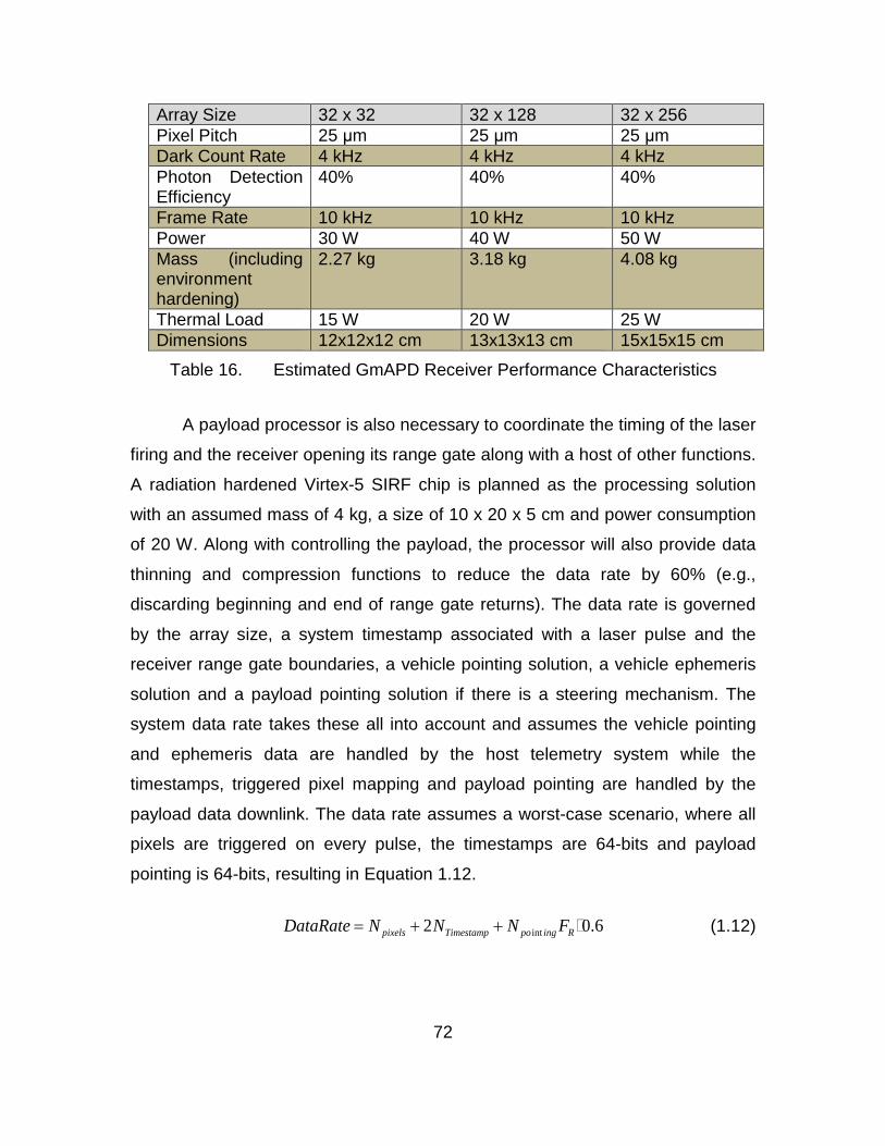
Array Size 32 x 32 32 x 128 32 x 256 Pixel Pitch 25 μm 25 μm 25 μm Dark Count Rate 4 kHz 4 kHz 4 kHz Photon Detection Efficiency
40% 40% 40%
Frame Rate 10 kHz 10 kHz 10 kHz Power 30 W 40 W 50 W Mass (including environment hardening)
2.27 kg 3.18 kg 4.08 kg
Thermal Load 15 W 20 W 25 W Dimensions 12x12x12 cm 13x13x13 cm 15x15x15 cm
Table 16. Estimated GmAPD Receiver Performance Characteristics
A payload processor is also necessary to coordinate the timing of the laser
firing and the receiver opening its range gate along with a host of other functions.
A radiation hardened Virtex-5 SIRF chip is planned as the processing solution
with an assumed mass of 4 kg, a size of 10 x 20 x 5 cm and power consumption
of 20 W. Along with controlling the payload, the processor will also provide data
thinning and compression functions to reduce the data rate by 60% (e.g.,
discarding beginning and end of range gate returns). The data rate is governed
by the array size, a system timestamp associated with a laser pulse and the
receiver range gate boundaries, a vehicle pointing solution, a vehicle ephemeris
solution and a payload pointing solution if there is a steering mechanism. The
system data rate takes these all into account and assumes the vehicle pointing
and ephemeris data are handled by the host telemetry system while the
timestamps, triggered pixel mapping and payload pointing are handled by the
payload data downlink. The data rate assumes a worst-case scenario, where all
pixels are triggered on every pulse, the timestamps are 64-bits and payload
pointing is 64-bits, resulting in Equation 1.12.
int2 0.6pixels Timestamp po ing RDataRate N N N F= + + (1.12)
72
3. Thermal Assumptions
With the potential for high heat loads due to the inefficiency of the laser
transmitters, thermal dissipation must be taken into account. Both silvered Teflon
and aluminized kapton, at an emissivity of 0.9, can reject a substantial amount of
heat and are standard materials for spacecraft thermal radiators. The main
radiator is assumed to operate at room temperature (298K) and deep space
facing. Equation 1.13 calculates the heat dissipation power of a radiator with
surface area A, emittance of ε, operating at an absolute temperature in Kelvin of
T and all multiplied by the Stephan-Boltzmann constant of σ. According to the
equation, the total thermal dissipation of the radiators per meter is calculated to
be 402 W/m2. In addition to the transmitter radiators, the detectors are run at 240
K with a single-stage thermoelectric cooler. At 240 K, a secondary radiator is
needed with a heat dissipation of 169 W/m2.
(1.13)
4. Telescope Mass Assumptions
The telescope aperture, playing a key role in the link budget equation, is
the main driver for the payload mass and volume. Combining both the Stahl
parametric cost equation based on diameter and equation based on mass, an
estimated OTA mass can be calculated based upon diameter (Equation 1.15).
(1.14)
(1.15)
5. Mission Assumptions
A number of assumptions are also made within the link budget equation
and mission space that will aid in the determination of transmitter power required
and area collection rates. The LIDAR target is assumed to be lambertian or
isotropically scattering due to the anticipated surface roughness of most non-
man-made objects at 1064 nm, the transmitter frequency. Highly polished and
glossy materials may have different scattering properties (non-isotropic) and will
73
not be evaluated as part of this model. The hemispherical reflectivity of the target
is assumed to be a conservative 20% based upon previous experiences with
airborne LIDAR testing. Foliage, man-made targets, ice sheets, etc., all maintain
individual reflectivities at the wavelength chosen and span a wide range of
values, requiring a simplification for the purposes of this thesis. The efficiency of
the transmit optics is assumed to be 95%, due to additional refractive optics and
collimators that may be necessary. The efficiency of the receive optics is
assumed to be 75% due to inefficiencies in the reflective optics, telescope
obscuration and any filters and folding optics. The fill factor of the detectors is
assumed to be 80%, due to the inefficiency of the GmAPD lenslets. At nadir, the
one-way atmospheric transmission of the 1064nm wavelength is 94%.
Accounting for these assumptions, the link budget equation then becomes:
62
0.20 0.942(1.064 10 )(0.95)(0.75) (0.80) (0.40)telPE P
pixels
AN Ehc N Rπ
−= (1.16)
Additional assumptions are required to determine area collection rates and
optimize the space-based LIDAR solutions. With GmAPDs, only one
photoelectron can be detected per pixel per range gate, therefore if more than
one photoelectron were to be generated, transmitter power would be wasted. To
optimize the system’s efficiency, the number of expected photoelectrons per pixel
per pulse should be tuned to between 0.2 and 0.3, reducing the likelihood that
two transmitted photons would arrive at the detector and trigger photoelectrons.
For link budget purposes and to increase the probability of detection in the
presence of noise, the number of photoelectrons per pixel per pulse is set at 0.3.
To determine area coverage rates, the number of detections per surface must be
set and account for noise factors and returns from atmospheric particulates.
Historical airborne LIDAR data have demonstrated that the minimum number of
detections per surface to perform coincident processing is between 3 and 6. In
order to remain conservative, the number of detections per surface or GSD will
be set at 6. With 6 detections necessary for a surface detection and 0.3
photoelectrons per pixel per pulse anticipated, 20 pulses would be required to
74
close the link in a noiseless environment. While noise and false returns represent
a very small potential number of photoelectrons, to combat this, a margin of 10X
is levied on the system, requiring 50 pulses to resolve a surface. With the
number of samples required per GSD, the area collection rate can now be
determined assuming a uniform beam distribution on the detector (Equation
1.17).
samples
pixels
prfACR NGSD N
=
(1.17)
1000050
pixels
ACR
GSD N
=
(1.18)
75

THIS PAGE INTENTIONALLY LEFT BLANK
76
VII. LIDAR SYSTEM DESIGN AND COSTS
A. IRIDIUM HOSTED PAYLOAD DESIGN
The Iridium Hosted Payload may be the lowest cost solution by leveraging
the already procured host bus and ground infrastructure, however hosting
considerations limit the size, mass and power of the payload substantially. The
volume constraint is one of the most stringent, requiring an optic of less than 1
meter with little room for the transmitter and receiver. The payload mass and
power parameters further restrict this active system, beyond a usable point.
1. 32x32 Array Detector-Based Payload Design
At 780 km in altitude, a number of trades were made to determine, for a
fixed detector (32x32) and a varying number of transmit fibers, the aperture
diameter needed to close the link budget. The assumptions from previous
chapters were used and the corresponding mass and power requirements were
calculated. Figures 28 and 29 portray the mass and power of the payload as the
number of fiber lasers is decreased. The increase in mass is due to the need to
maintain 0.3 photons per pixel per pulse at each of the 1024 detector elements,
requiring the aperture size to compensate for the reduced transmit power and
thereby increasing the mass substantially. None of the trades for a 32x32 array
satisfy the Iridium NEXT hosted payload parameters. With the transmitter driving
power requirements, there are very few options that could be sustained at 100%
duty cycle. Reducing the duty cycle to 10%, all of the transmitter options studied
meet the Iridium power requirements with at least 2X power margin. Looking at
Figure 29 again, however, it becomes apparent that all potential payload options
exceed the 50 kg mass requirement by 2X. Figure 30 shows the major mass
driver, the receive optics, and its relationship with payload mass.
77
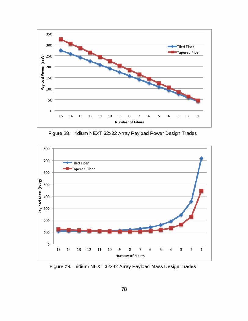
Figure 28. Iridium NEXT 32x32 Array Payload Power Design Trades
Figure 29. Iridium NEXT 32x32 Array Payload Mass Design Trades
78
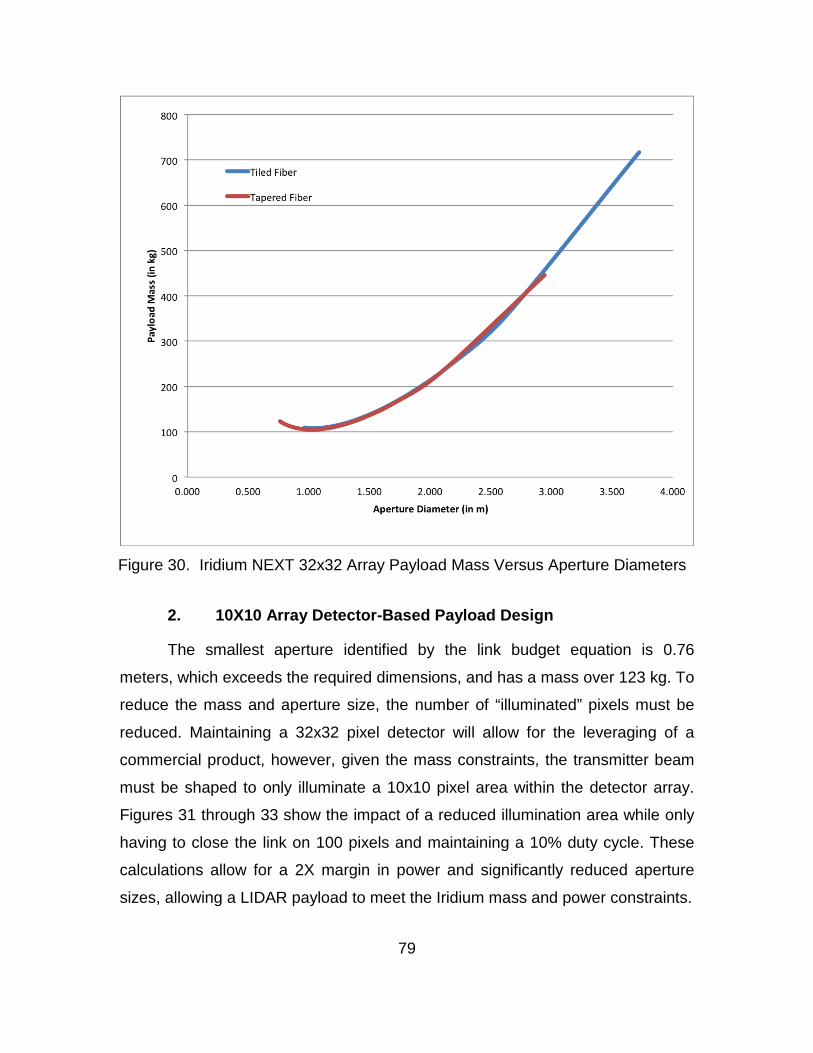
Figure 30. Iridium NEXT 32x32 Array Payload Mass Versus Aperture Diameters
2. 10X10 Array Detector-Based Payload Design
The smallest aperture identified by the link budget equation is 0.76
meters, which exceeds the required dimensions, and has a mass over 123 kg. To
reduce the mass and aperture size, the number of “illuminated” pixels must be
reduced. Maintaining a 32x32 pixel detector will allow for the leveraging of a
commercial product, however, given the mass constraints, the transmitter beam
must be shaped to only illuminate a 10x10 pixel area within the detector array.
Figures 31 through 33 show the impact of a reduced illumination area while only
having to close the link on 100 pixels and maintaining a 10% duty cycle. These
calculations allow for a 2X margin in power and significantly reduced aperture
sizes, allowing a LIDAR payload to meet the Iridium mass and power constraints.
79
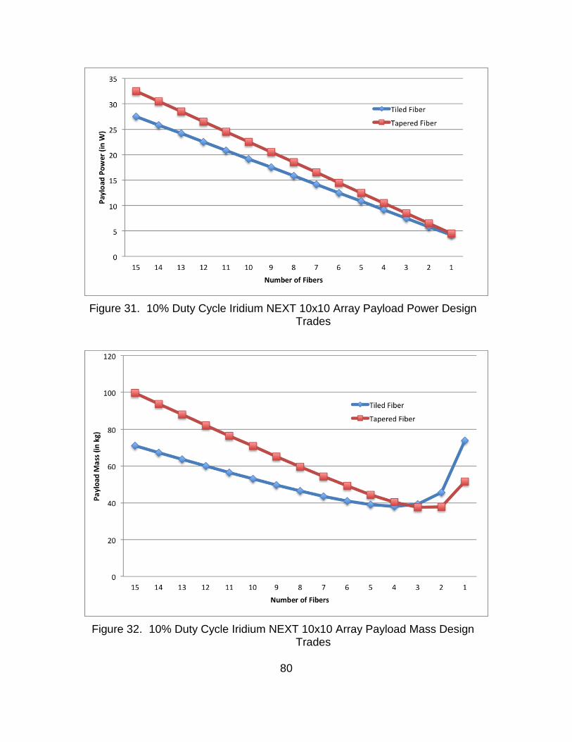
Figure 31. 10% Duty Cycle Iridium NEXT 10x10 Array Payload Power Design
Trades
Figure 32. 10% Duty Cycle Iridium NEXT 10x10 Array Payload Mass Design
Trades
80
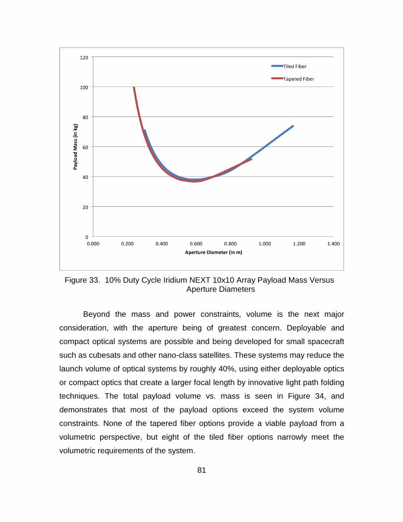
Figure 33. 10% Duty Cycle Iridium NEXT 10x10 Array Payload Mass Versus
Aperture Diameters
Beyond the mass and power constraints, volume is the next major
consideration, with the aperture being of greatest concern. Deployable and
compact optical systems are possible and being developed for small spacecraft
such as cubesats and other nano-class satellites. These systems may reduce the
launch volume of optical systems by roughly 40%, using either deployable optics
or compact optics that create a larger focal length by innovative light path folding
techniques. The total payload volume vs. mass is seen in Figure 34, and
demonstrates that most of the payload options exceed the system volume
constraints. None of the tapered fiber options provide a viable payload from a
volumetric perspective, but eight of the tiled fiber options narrowly meet the
volumetric requirements of the system.
81
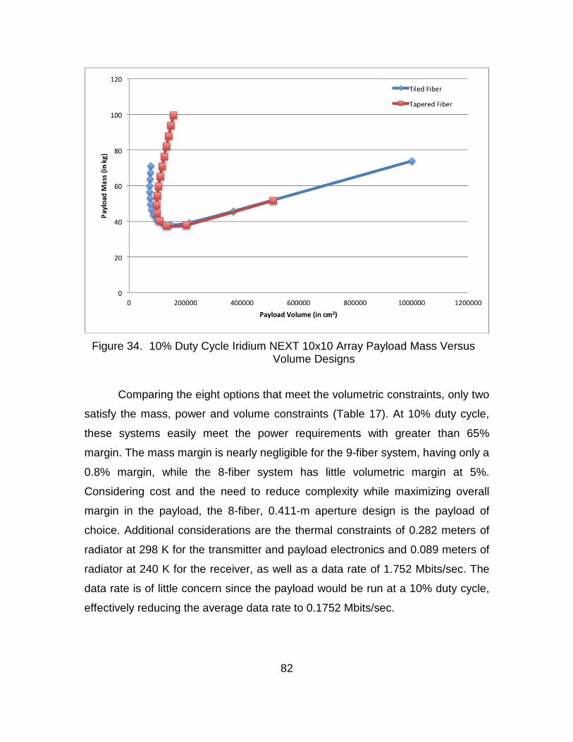
Figure 34. 10% Duty Cycle Iridium NEXT 10x10 Array Payload Mass Versus
Volume Designs
Comparing the eight options that meet the volumetric constraints, only two
satisfy the mass, power and volume constraints (Table 17). At 10% duty cycle,
these systems easily meet the power requirements with greater than 65%
margin. The mass margin is nearly negligible for the 9-fiber system, having only a
0.8% margin, while the 8-fiber system has little volumetric margin at 5%.
Considering cost and the need to reduce complexity while maximizing overall
margin in the payload, the 8-fiber, 0.411-m aperture design is the payload of
choice. Additional considerations are the thermal constraints of 0.282 meters of
radiator at 298 K for the transmitter and payload electronics and 0.089 meters of
radiator at 240 K for the receiver, as well as a data rate of 1.752 Mbits/sec. The
data rate is of little concern since the payload would be run at a 10% duty cycle,
effectively reducing the average data rate to 0.1752 Mbits/sec.
82
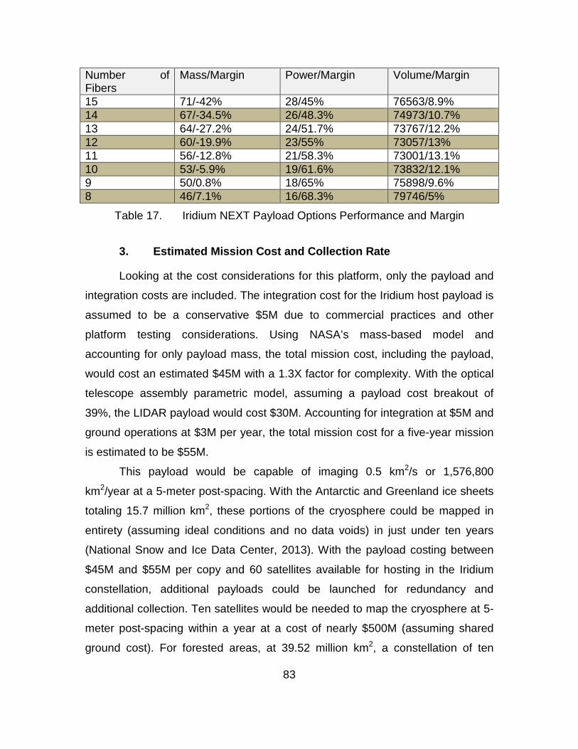
Number of Fibers
Mass/Margin Power/Margin Volume/Margin
15 71/-42% 28/45% 76563/8.9% 14 67/-34.5% 26/48.3% 74973/10.7% 13 64/-27.2% 24/51.7% 73767/12.2% 12 60/-19.9% 23/55% 73057/13% 11 56/-12.8% 21/58.3% 73001/13.1% 10 53/-5.9% 19/61.6% 73832/12.1% 9 50/0.8% 18/65% 75898/9.6% 8 46/7.1% 16/68.3% 79746/5%
Table 17. Iridium NEXT Payload Options Performance and Margin
3. Estimated Mission Cost and Collection Rate
Looking at the cost considerations for this platform, only the payload and
integration costs are included. The integration cost for the Iridium host payload is
assumed to be a conservative $5M due to commercial practices and other
platform testing considerations. Using NASA’s mass-based model and
accounting for only payload mass, the total mission cost, including the payload,
would cost an estimated $45M with a 1.3X factor for complexity. With the optical
telescope assembly parametric model, assuming a payload cost breakout of
39%, the LIDAR payload would cost $30M. Accounting for integration at $5M and
ground operations at $3M per year, the total mission cost for a five-year mission
is estimated to be $55M.
This payload would be capable of imaging 0.5 km2/s or 1,576,800
km2/year at a 5-meter post-spacing. With the Antarctic and Greenland ice sheets
totaling 15.7 million km2, these portions of the cryosphere could be mapped in
entirety (assuming ideal conditions and no data voids) in just under ten years
(National Snow and Ice Data Center, 2013). With the payload costing between
$45M and $55M per copy and 60 satellites available for hosting in the Iridium
constellation, additional payloads could be launched for redundancy and
additional collection. Ten satellites would be needed to map the cryosphere at 5-
meter post-spacing within a year at a cost of nearly $500M (assuming shared
ground cost). For forested areas, at 39.52 million km2, a constellation of ten
83
hosted payloads would be able to provide 5-meter post-spacing for forest carbon
monitoring projects within 2.5 additional years (Nabuurs & Masera, 2007). The
USGS mission of 1-meter post-spacing for the United States, at 9,147,420 km2,
would reduce the area collection rate to 0.02 km2/s or 630,720 km2/year per
payload, requiring 15 payloads to map the United States within a year (The
World Bank, 2013). While this may be costly at over $885M, a smaller
constellation could help map more expensive mapping areas and could be
included in the cost-benefit analysis for future elevation data studies.
84
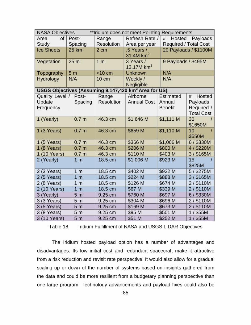
NASA Objectives **Iridium does not meet Pointing Requirements Area of Study
Post-Spacing
Range Resolution
Refresh Rate / Area per year
# Hosted Payloads Required / Total Cost
Ice Sheets 25 km 2 cm .5 Years / 31.4M km2
20 Payloads / $1100M
Vegetation 25 m 1 m 3 Years / 13.17M km2
9 Payloads / $495M
Topography 5 m <10 cm Unknown N/A Hydrology N/A 10 cm Weekly /
Negligible N/A
USGS Objectives (Assuming 9,147,420 km2 Area for US) Quality Level / Update Frequency
Post-Spacing
Range Resolution
Airborne Annual Cost
Estimated Annual Benefit
# Hosted Payloads Required / Total Cost
1 (Yearly) 0.7 m 46.3 cm $1,646 M $1,111 M 30 / $1650M
1 (3 Years) 0.7 m 46.3 cm $659 M $1,110 M 10 / $550M
1 (5 Years) 0.7 m 46.3 cm $366 M $1,066 M 6 / $330M 1 (8 Years) 0.7 m 46.3 cm $206 M $800 M 4 / $220M 1 (10 Years) 0.7 m 46.3 cm $110 M $403 M 3 / $165M 2 (Yearly) 1 m 18.5 cm $1,006 M $923 M 15 /
$825M 2 (3 Years) 1 m 18.5 cm $402 M $922 M 5 / $275M 2 (5 Years) 1 m 18.5 cm $224 M $888 M 3 / $165M 2 (8 Years) 1 m 18.5 cm $126 M $674 M 2 / $110M 2 (10 Years) 1 m 18.5 cm $67 M $339 M 2 / $110M 3 (Yearly) 5 m 9.25 cm $760 M $697 M 6 / $330M 3 (3 Years) 5 m 9.25 cm $304 M $696 M 2 / $110M 3 (5 Years) 5 m 9.25 cm $169 M $673 M 2 / $110M 3 (8 Years) 5 m 9.25 cm $95 M $501 M 1 / $55M 3 (10 Years) 5 m 9.25 cm $51 M $252 M 1 / $55M
Table 18. Iridium Fulfillment of NASA and USGS LIDAR Objectives
The Iridium hosted payload option has a number of advantages and
disadvantages. Its low initial cost and redundant spacecraft make it attractive
from a risk reduction and revisit rate perspective. It would also allow for a gradual
scaling up or down of the number of systems based on insights gathered from
the data and could be more resilient from a budgetary planning perspective than
one large program. Technology advancements and payload fixes could also be 85
included as new payloads are built. There are, however, some disadvantages of
Iridium hosted payloads. The bus does not meet the pointing knowledge and
accuracy requirements, making the geolocation of LIDAR returns in 3-D space
more difficult. This may be alleviated through additional attitude determination
hardware such as gyros, which would increase pointing knowledge but possibly
not accuracy. While the number of hosted payloads required is high to meet the
NASA objectives, the system is collecting at 5-meter post spacing. The number
of satellites could be reduced if the data was down-sampled to the objective post
spacing and a smaller number of returns were expected per detector IFOV.
For the USGS objectives, the Iridium hosted payload has a number of
attractive options at different quality levels. Depending on the lifetime of each
satellite and its LIDAR payload, the monetary benefits of a space-based
approach could outweigh that of the airborne approach. In Table 18, the airborne
costs are per year, however the hosted payload costs may include multiple years
of operation. With an estimated five-year lifetime for the payload, the Iridium
hosted option could provide a five times greater return on investment than the
airborne options. Taking into account NASA and USGS’s objectives and
assuming down-sampling is possible, ice sheets sampled at a 1-km post spacing
would only need one satellite to fulfill the requirement and would be limited by
spacecraft speed and orbital constraints. For vegetation, at a down-sampled
25-m post spacing, only two hosted payloads would be required and could also
subsume the ice sheet measurements as well. For USGS requirements, the
highest returns on investment are for the 0.7-m post spacing with updates every
three years and 0.7-m post spacing with updates every five years. Updating the
USGS elevation data set every three years would require ten payloads at a cost
of $550M, while over the course of five years providing a return of $5,550M.
Updating the data set every five years would require six payloads at a cost of
$330M, while providing a return of $5,330M.
Taking into account total mission costs of less than $250M and $500M, a
constellation of four and nine payloads could be chosen, respectively. With a
86
four-payload constellation, two would be reserved for NASA objectives and the
capacity of the other two could fulfill USGS objectives providing a return on
investment of $3,480M over five years with a 5-m post spacing and updates
every three years. With a nine payload constellation, two would again be
reserved for NASA objectives and the capacity of the other seven could provide a
return on investment of $5,330M over five years with a 0.7-m post spacing and
updates every five years.
B. FREE-FLIER SATELLITE DESIGNS
Free flyer payloads offer additional flexibility over hosted payloads that
can increase mission performance, but introduce a number of other costs that
require consideration (e.g., launch, bus, full test and integration, program
management). Two options will be explored for both a low-cost small satellite
(less than $250M) and a mid-cost larger satellite (less than $500M) for the LIDAR
mission. Exploring the NASA cost model and associated standard buses, there
are a number of options that satisfy both cost points.
1. Low Cost: Less than $250M Satellite Design
The low-cost small satellite must balance both the mission life of the bus
and the associated cost. Two methods are used to determine the overall cost of
the system. First, an aperture-based approach is used which uses standard
detector sizes (32x32, 32x128 and 32x256) and a varying number of lasers with
associated powers. From here, the aperture size is determined by closing the link
for each pixel of the array. Larger apertures are needed for large arrays with a
small number of lasers, while smaller detector arrays with a large number of
lasers need smaller apertures to close the link. After determining the aperture
sizes commensurate with a less than $250M mission, these constraints are
applied to the mass-based model. Only if the two models agree that the cost is
below $250M, will the satellite design be accepted.
A number of iterations were completed to determine the potential options
for a less than $250M mission based on the aperture cost model. The number of
87
lasers was limited from one to fifteen due to the need to limit the system
complexity. All three detector sizes were modeled, but even at a maximum of 15
lasers, both the 32x128 and 32x256 detectors had aperture sizes that, when run
through the cost model, exceeded the $250M mark. The 32x128 detector was
only able to close the link with a minimum aperture size of 1.169 meters and a
spacecraft cost of $370.568M. The 32x256 detector was only able to close the
link with a minimum aperture size of 1.653 meters and a spacecraft cost of
$623.218M. The 32x32 detector is the only detector that was able to be fully
illuminated and had a number of aperture sizes that satisfied the less than
$250M cost ceiling. In Figure 35, the aperture-based cost model curves are
shown for the 32x32 detector. Both the tapered and tiled lasers look to satisfy the
constraints with a number of options. Due to the benefits of increased power with
the tapered lasers, only these lasers were considered in the mass-based
estimates. For the tapered lasers, the seven to fifteen laser range was able to
satisfy the cost constraints with aperture sizes ranging from 0.856 to 0.584
meters and costs ranging from $232.042M to $131.015M, respectively. These
choices were then used to limit the iterations needed on the mass-based model.
88
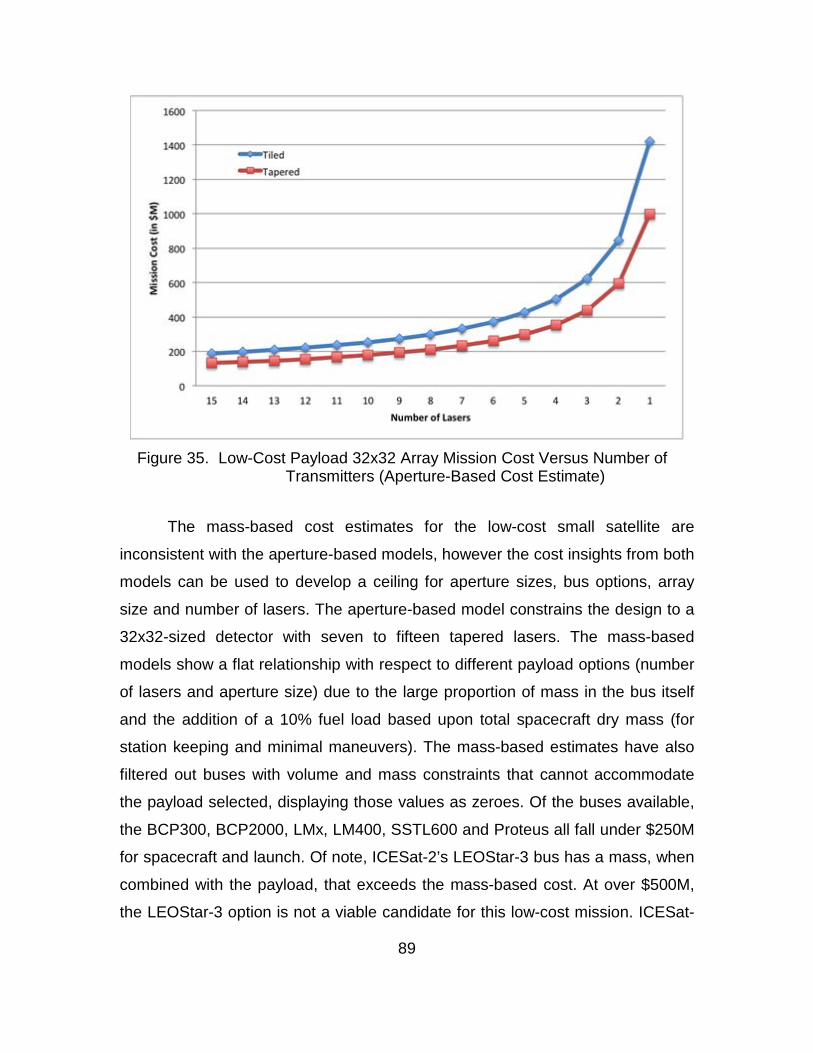
Figure 35. Low-Cost Payload 32x32 Array Mission Cost Versus Number of
Transmitters (Aperture-Based Cost Estimate)
The mass-based cost estimates for the low-cost small satellite are
inconsistent with the aperture-based models, however the cost insights from both
models can be used to develop a ceiling for aperture sizes, bus options, array
size and number of lasers. The aperture-based model constrains the design to a
32x32-sized detector with seven to fifteen tapered lasers. The mass-based
models show a flat relationship with respect to different payload options (number
of lasers and aperture size) due to the large proportion of mass in the bus itself
and the addition of a 10% fuel load based upon total spacecraft dry mass (for
station keeping and minimal maneuvers). The mass-based estimates have also
filtered out buses with volume and mass constraints that cannot accommodate
the payload selected, displaying those values as zeroes. Of the buses available,
the BCP300, BCP2000, LMx, LM400, SSTL600 and Proteus all fall under $250M
for spacecraft and launch. Of note, ICESat-2’s LEOStar-3 bus has a mass, when
combined with the payload, that exceeds the mass-based cost. At over $500M,
the LEOStar-3 option is not a viable candidate for this low-cost mission. ICESat-
89
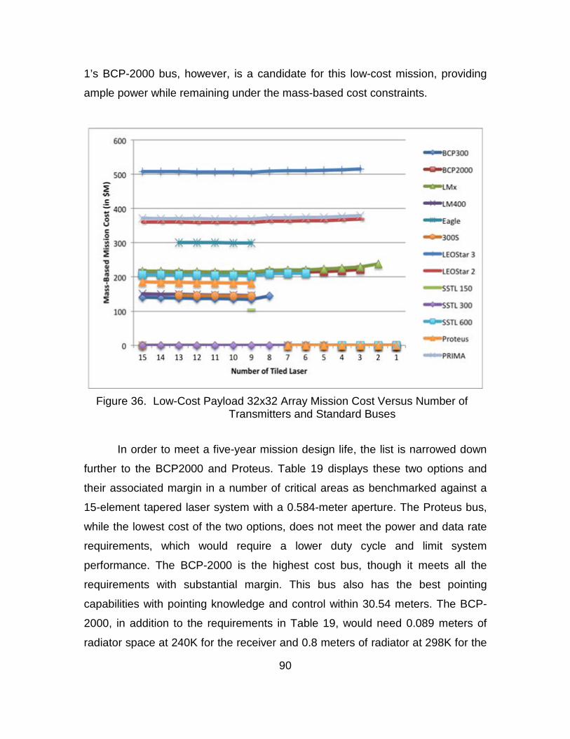
1’s BCP-2000 bus, however, is a candidate for this low-cost mission, providing
ample power while remaining under the mass-based cost constraints.
Figure 36. Low-Cost Payload 32x32 Array Mission Cost Versus Number of
Transmitters and Standard Buses
In order to meet a five-year mission design life, the list is narrowed down
further to the BCP2000 and Proteus. Table 19 displays these two options and
their associated margin in a number of critical areas as benchmarked against a
15-element tapered laser system with a 0.584-meter aperture. The Proteus bus,
while the lowest cost of the two options, does not meet the power and data rate
requirements, which would require a lower duty cycle and limit system
performance. The BCP-2000 is the highest cost bus, though it meets all the
requirements with substantial margin. This bus also has the best pointing
capabilities with pointing knowledge and control within 30.54 meters. The BCP-
2000, in addition to the requirements in Table 19, would need 0.089 meters of
radiator space at 240K for the receiver and 0.8 meters of radiator at 298K for the
90
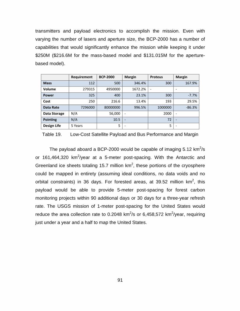
transmitters and payload electronics to accomplish the mission. Even with
varying the number of lasers and aperture size, the BCP-2000 has a number of
capabilities that would significantly enhance the mission while keeping it under
$250M ($216.6M for the mass-based model and $131.015M for the aperture-
based model).
Requirement BCP-2000 Margin Proteus Margin Mass 112 500 346.4% 300 167.9% Volume 279315 4950000 1672.2% - - Power 325 400 23.1% 300 -7.7% Cost 250 216.6 13.4% 193 29.5% Data Rate 7296000 80000000 996.5% 1000000 -86.3% Data Storage N/A 56,000 - 2000 - Pointing N/A 10.5 - 72 - Design Life 5 Years 5 - 5 -
Table 19. Low-Cost Satellite Payload and Bus Performance and Margin
The payload aboard a BCP-2000 would be capable of imaging 5.12 km2/s
or 161,464,320 km2/year at a 5-meter post-spacing. With the Antarctic and
Greenland ice sheets totaling 15.7 million km2, these portions of the cryosphere
could be mapped in entirety (assuming ideal conditions, no data voids and no
orbital constraints) in 36 days. For forested areas, at 39.52 million km2, this
payload would be able to provide 5-meter post-spacing for forest carbon
monitoring projects within 90 additional days or 30 days for a three-year refresh
rate. The USGS mission of 1-meter post-spacing for the United States would
reduce the area collection rate to 0.2048 km2/s or 6,458,572 km2/year, requiring
just under a year and a half to map the United States.
91
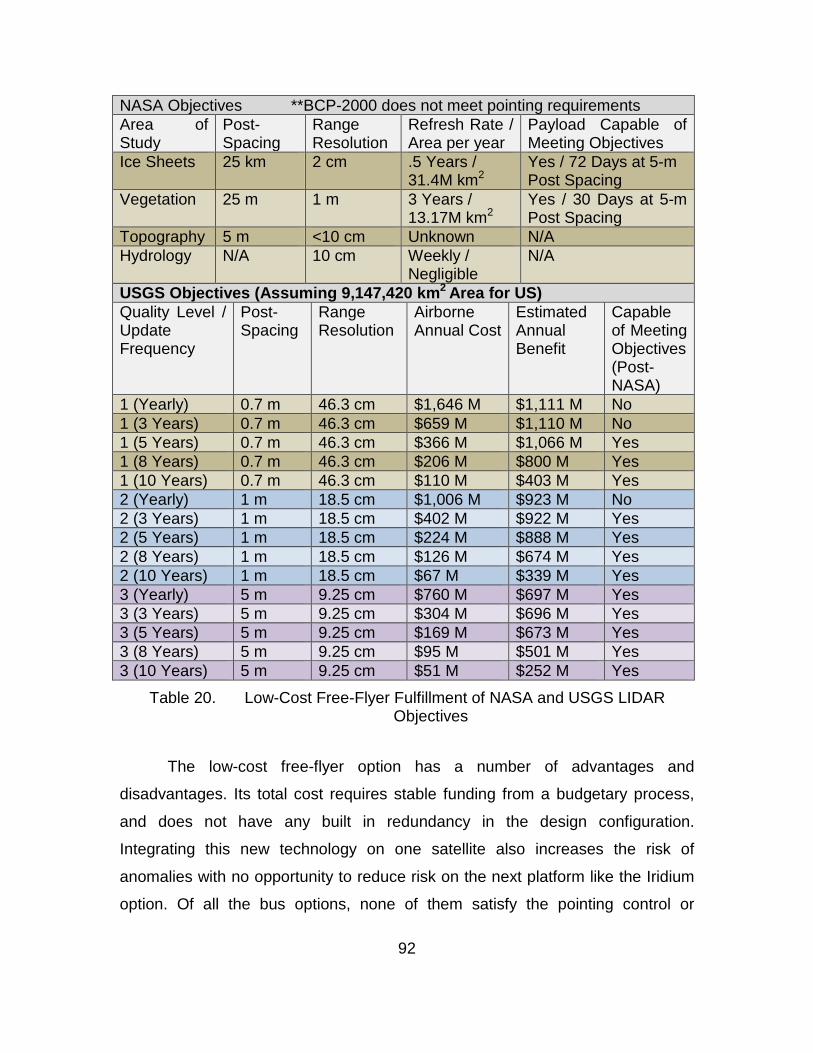
NASA Objectives **BCP-2000 does not meet pointing requirements Area of Study
Post-Spacing
Range Resolution
Refresh Rate / Area per year
Payload Capable of Meeting Objectives
Ice Sheets 25 km 2 cm .5 Years / 31.4M km2
Yes / 72 Days at 5-m Post Spacing
Vegetation 25 m 1 m 3 Years / 13.17M km2
Yes / 30 Days at 5-m Post Spacing
Topography 5 m <10 cm Unknown N/A Hydrology N/A 10 cm Weekly /
Negligible N/A
USGS Objectives (Assuming 9,147,420 km2 Area for US) Quality Level / Update Frequency
Post-Spacing
Range Resolution
Airborne Annual Cost
Estimated Annual Benefit
Capable of Meeting Objectives (Post-NASA)
1 (Yearly) 0.7 m 46.3 cm $1,646 M $1,111 M No 1 (3 Years) 0.7 m 46.3 cm $659 M $1,110 M No 1 (5 Years) 0.7 m 46.3 cm $366 M $1,066 M Yes 1 (8 Years) 0.7 m 46.3 cm $206 M $800 M Yes 1 (10 Years) 0.7 m 46.3 cm $110 M $403 M Yes 2 (Yearly) 1 m 18.5 cm $1,006 M $923 M No 2 (3 Years) 1 m 18.5 cm $402 M $922 M Yes 2 (5 Years) 1 m 18.5 cm $224 M $888 M Yes 2 (8 Years) 1 m 18.5 cm $126 M $674 M Yes 2 (10 Years) 1 m 18.5 cm $67 M $339 M Yes 3 (Yearly) 5 m 9.25 cm $760 M $697 M Yes 3 (3 Years) 5 m 9.25 cm $304 M $696 M Yes 3 (5 Years) 5 m 9.25 cm $169 M $673 M Yes 3 (8 Years) 5 m 9.25 cm $95 M $501 M Yes 3 (10 Years) 5 m 9.25 cm $51 M $252 M Yes
Table 20. Low-Cost Free-Flyer Fulfillment of NASA and USGS LIDAR Objectives
The low-cost free-flyer option has a number of advantages and
disadvantages. Its total cost requires stable funding from a budgetary process,
and does not have any built in redundancy in the design configuration.
Integrating this new technology on one satellite also increases the risk of
anomalies with no opportunity to reduce risk on the next platform like the Iridium
option. Of all the bus options, none of them satisfy the pointing control or
92
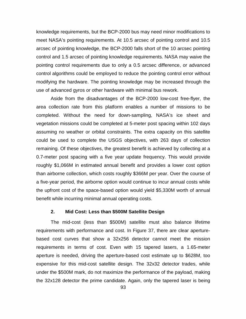
knowledge requirements, but the BCP-2000 bus may need minor modifications to
meet NASA’s pointing requirements. At 10.5 arcsec of pointing control and 10.5
arcsec of pointing knowledge, the BCP-2000 falls short of the 10 arcsec pointing
control and 1.5 arcsec of pointing knowledge requirements. NASA may waive the
pointing control requirements due to only a 0.5 arcsec difference, or advanced
control algorithms could be employed to reduce the pointing control error without
modifying the hardware. The pointing knowledge may be increased through the
use of advanced gyros or other hardware with minimal bus rework.
Aside from the disadvantages of the BCP-2000 low-cost free-flyer, the
area collection rate from this platform enables a number of missions to be
completed. Without the need for down-sampling, NASA’s ice sheet and
vegetation missions could be completed at 5-meter post spacing within 102 days
assuming no weather or orbital constraints. The extra capacity on this satellite
could be used to complete the USGS objectives, with 263 days of collection
remaining. Of these objectives, the greatest benefit is achieved by collecting at a
0.7-meter post spacing with a five year update frequency. This would provide
roughly $1,066M in estimated annual benefit and provides a lower cost option
than airborne collection, which costs roughly $366M per year. Over the course of
a five-year period, the airborne option would continue to incur annual costs while
the upfront cost of the space-based option would yield $5,330M worth of annual
benefit while incurring minimal annual operating costs.
2. Mid Cost: Less than $500M Satellite Design
The mid-cost (less than $500M) satellite must also balance lifetime
requirements with performance and cost. In Figure 37, there are clear aperture-
based cost curves that show a 32x256 detector cannot meet the mission
requirements in terms of cost. Even with 15 tapered lasers, a 1.65-meter
aperture is needed, driving the aperture-based cost estimate up to $628M, too
expensive for this mid-cost satellite design. The 32x32 detector trades, while
under the $500M mark, do not maximize the performance of the payload, making
the 32x128 detector the prime candidate. Again, only the tapered laser is being 93
modeled and a maximum of 15 lasers are being considered, resulting in Figure
38 for the 32x128 detector.
Figure 37. Mid-Cost Payload 32x256 Array Mission Cost Versus Number of
Transmitters (Aperture-based Cost Estimate)
94
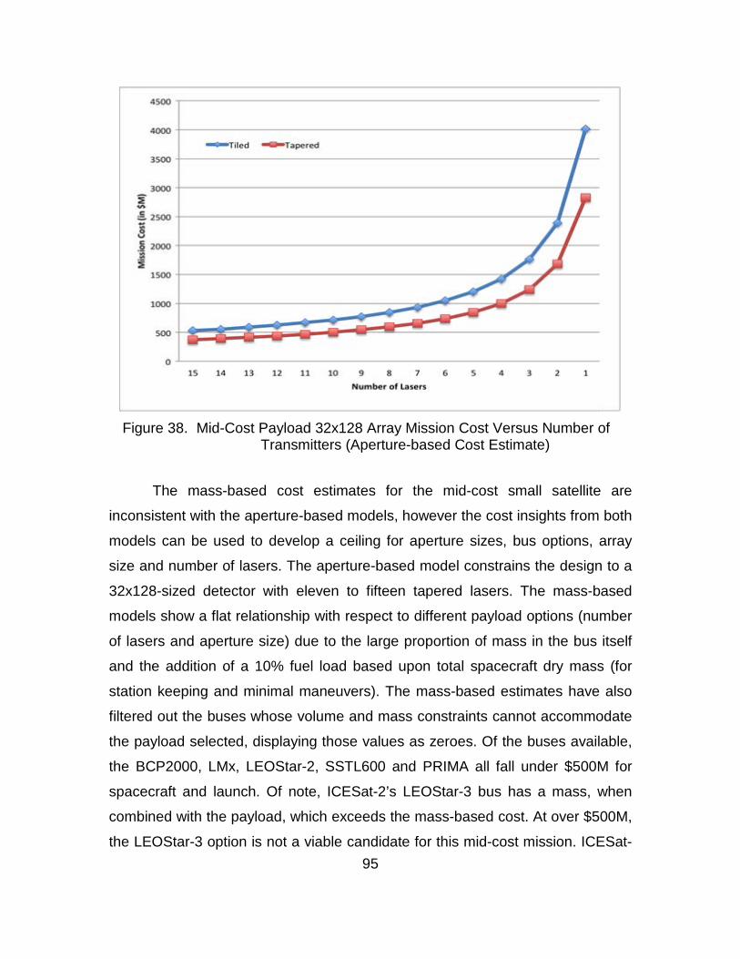
Figure 38. Mid-Cost Payload 32x128 Array Mission Cost Versus Number of
Transmitters (Aperture-based Cost Estimate)
The mass-based cost estimates for the mid-cost small satellite are
inconsistent with the aperture-based models, however the cost insights from both
models can be used to develop a ceiling for aperture sizes, bus options, array
size and number of lasers. The aperture-based model constrains the design to a
32x128-sized detector with eleven to fifteen tapered lasers. The mass-based
models show a flat relationship with respect to different payload options (number
of lasers and aperture size) due to the large proportion of mass in the bus itself
and the addition of a 10% fuel load based upon total spacecraft dry mass (for
station keeping and minimal maneuvers). The mass-based estimates have also
filtered out the buses whose volume and mass constraints cannot accommodate
the payload selected, displaying those values as zeroes. Of the buses available,
the BCP2000, LMx, LEOStar-2, SSTL600 and PRIMA all fall under $500M for
spacecraft and launch. Of note, ICESat-2’s LEOStar-3 bus has a mass, when
combined with the payload, which exceeds the mass-based cost. At over $500M,
the LEOStar-3 option is not a viable candidate for this mid-cost mission. ICESat- 95
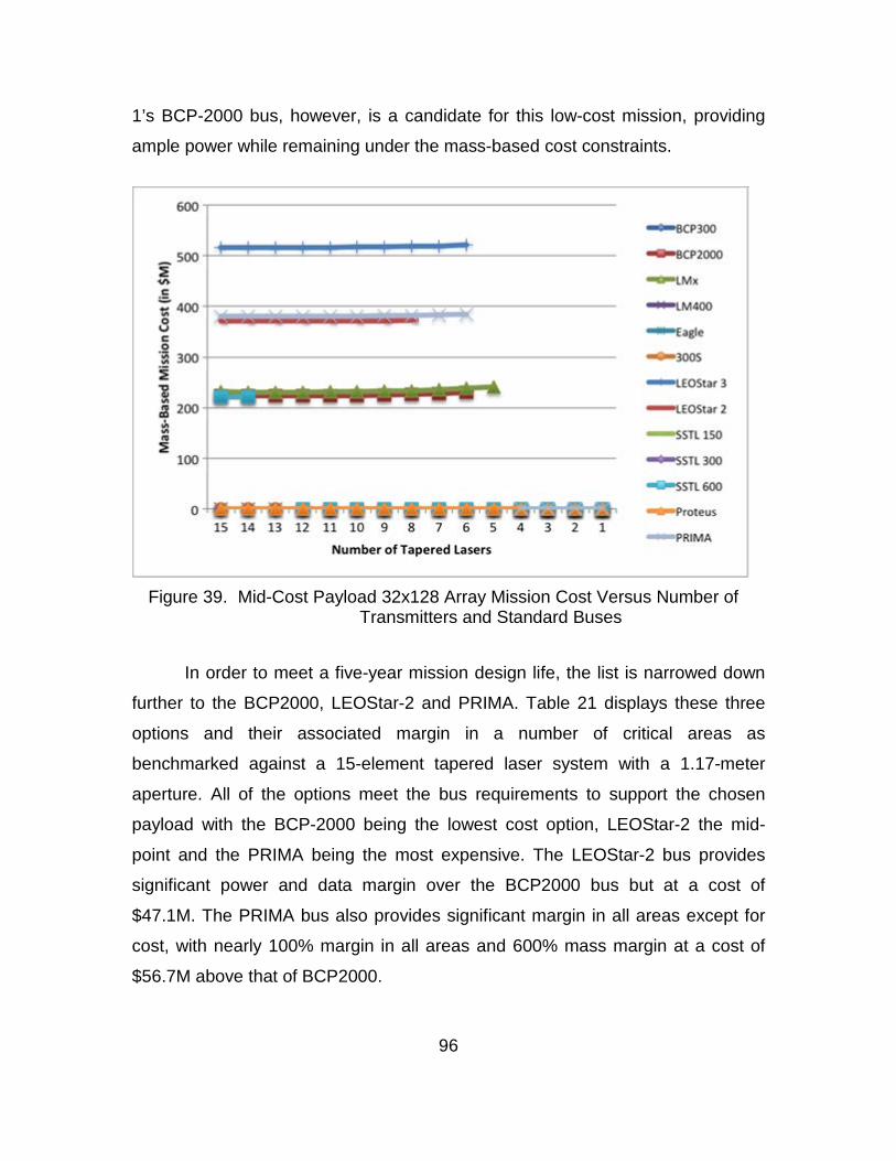
1’s BCP-2000 bus, however, is a candidate for this low-cost mission, providing
ample power while remaining under the mass-based cost constraints.
Figure 39. Mid-Cost Payload 32x128 Array Mission Cost Versus Number of
Transmitters and Standard Buses
In order to meet a five-year mission design life, the list is narrowed down
further to the BCP2000, LEOStar-2 and PRIMA. Table 21 displays these three
options and their associated margin in a number of critical areas as
benchmarked against a 15-element tapered laser system with a 1.17-meter
aperture. All of the options meet the bus requirements to support the chosen
payload with the BCP-2000 being the lowest cost option, LEOStar-2 the mid-
point and the PRIMA being the most expensive. The LEOStar-2 bus provides
significant power and data margin over the BCP2000 bus but at a cost of
$47.1M. The PRIMA bus also provides significant margin in all areas except for
cost, with nearly 100% margin in all areas and 600% mass margin at a cost of
$56.7M above that of BCP2000.
96
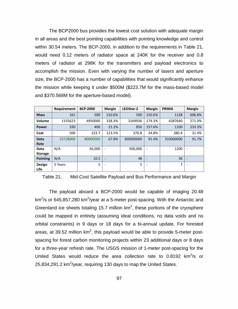
The BCP2000 bus provides the lowest cost solution with adequate margin
in all areas and the best pointing capabilities with pointing knowledge and control
within 30.54 meters. The BCP-2000, in addition to the requirements in Table 21,
would need 0.12 meters of radiator space at 240K for the receiver and 0.8
meters of radiator at 298K for the transmitters and payload electronics to
accomplish the mission. Even with varying the number of lasers and aperture
size, the BCP-2000 has a number of capabilities that would significantly enhance
the mission while keeping it under $500M ($223.7M for the mass-based model
and $370.568M for the aperture-based model).
Requirement BCP-2000 Margin LEOStar-2 Margin PRIMA Margin Mass 161 500 210.6% 500 210.6% 1138 606.8% Volume 1155623 4950000 328.3% 3169936 174.3% 4287640 271.0% Power 330 400 21.2% 850 157.6% 1100 233.3% Cost 500 223.7 123.5% 370.8 34.8% 380.4 31.4% Data Rate
25728000 80000000 67.8% 300000000 91.4% 310000000 91.7%
Data Storage
N/A 56,000 - 500,000 - 1200 -
Pointing N/A 10.5 - 48 - 36 - Design Life
5 Years 5 - 5 - 7 -
Table 21. Mid-Cost Satellite Payload and Bus Performance and Margin
The payload aboard a BCP-2000 would be capable of imaging 20.48
km2/s or 645,857,280 km2/year at a 5-meter post-spacing. With the Antarctic and
Greenland ice sheets totaling 15.7 million km2, these portions of the cryosphere
could be mapped in entirety (assuming ideal conditions, no data voids and no
orbital constraints) in 9 days or 18 days for a bi-annual update. For forested
areas, at 39.52 million km2, this payload would be able to provide 5-meter post-
spacing for forest carbon monitoring projects within 23 additional days or 8 days
for a three-year refresh rate. The USGS mission of 1-meter post-spacing for the
United States would reduce the area collection rate to 0.8192 km2/s or
25,834,291.2 km2/year, requiring 130 days to map the United States.
97
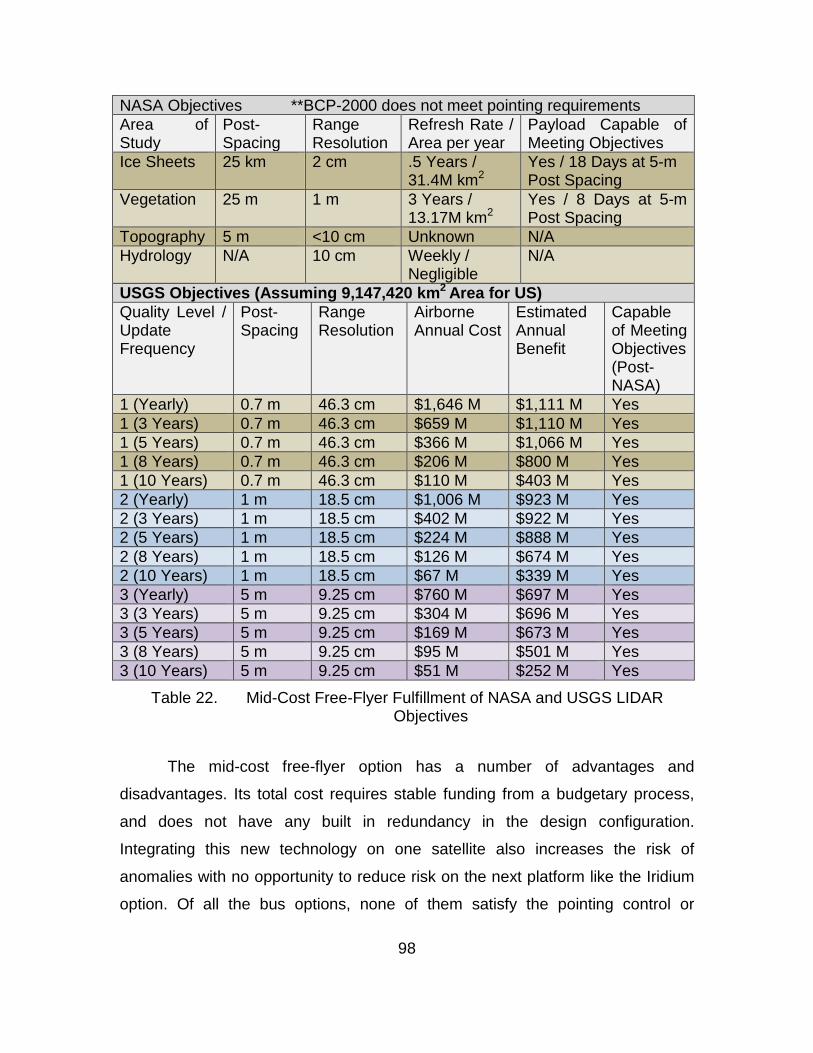
NASA Objectives **BCP-2000 does not meet pointing requirements Area of Study
Post-Spacing
Range Resolution
Refresh Rate / Area per year
Payload Capable of Meeting Objectives
Ice Sheets 25 km 2 cm .5 Years / 31.4M km2
Yes / 18 Days at 5-m Post Spacing
Vegetation 25 m 1 m 3 Years / 13.17M km2
Yes / 8 Days at 5-m Post Spacing
Topography 5 m <10 cm Unknown N/A Hydrology N/A 10 cm Weekly /
Negligible N/A
USGS Objectives (Assuming 9,147,420 km2 Area for US) Quality Level / Update Frequency
Post-Spacing
Range Resolution
Airborne Annual Cost
Estimated Annual Benefit
Capable of Meeting Objectives (Post-NASA)
1 (Yearly) 0.7 m 46.3 cm $1,646 M $1,111 M Yes 1 (3 Years) 0.7 m 46.3 cm $659 M $1,110 M Yes 1 (5 Years) 0.7 m 46.3 cm $366 M $1,066 M Yes 1 (8 Years) 0.7 m 46.3 cm $206 M $800 M Yes 1 (10 Years) 0.7 m 46.3 cm $110 M $403 M Yes 2 (Yearly) 1 m 18.5 cm $1,006 M $923 M Yes 2 (3 Years) 1 m 18.5 cm $402 M $922 M Yes 2 (5 Years) 1 m 18.5 cm $224 M $888 M Yes 2 (8 Years) 1 m 18.5 cm $126 M $674 M Yes 2 (10 Years) 1 m 18.5 cm $67 M $339 M Yes 3 (Yearly) 5 m 9.25 cm $760 M $697 M Yes 3 (3 Years) 5 m 9.25 cm $304 M $696 M Yes 3 (5 Years) 5 m 9.25 cm $169 M $673 M Yes 3 (8 Years) 5 m 9.25 cm $95 M $501 M Yes 3 (10 Years) 5 m 9.25 cm $51 M $252 M Yes
Table 22. Mid-Cost Free-Flyer Fulfillment of NASA and USGS LIDAR Objectives
The mid-cost free-flyer option has a number of advantages and
disadvantages. Its total cost requires stable funding from a budgetary process,
and does not have any built in redundancy in the design configuration.
Integrating this new technology on one satellite also increases the risk of
anomalies with no opportunity to reduce risk on the next platform like the Iridium
option. Of all the bus options, none of them satisfy the pointing control or
98
knowledge requirements, but the BCP-2000 bus may need minor modifications to
meet NASA’s pointing requirements. At 10.5 arcsec of pointing control and 10.5
arcsec of pointing knowledge, the BCP-2000 falls short of the 10 arcsec pointing
control and 1.5 arcsec of pointing knowledge requirements. NASA may waive the
pointing control requirements due to only a 0.5 arcsec difference, or advanced
control algorithms could be employed to reduce the pointing control error without
modifying the hardware. The pointing knowledge may be increased through the
use of advanced gyros or other hardware with minimal bus rework.
Aside from the disadvantages of the BCP-2000 low-cost free-flyer, the
area collection rate from this platform enables a number of missions to be
completed. Without the need for down-sampling, NASA’s ice sheet and
vegetation missions could be completed at 5-meter post spacing within 26 days
assuming no weather or orbital constraints. The extra capacity on this satellite
could be used to complete the USGS objectives, with 339 days of collection
remaining. Of these objectives, the greatest benefit is achieved by collecting at
0.7-meter post spacing with a one-year update frequency. This would provide
roughly $1,111M in estimated annual benefit and provides a lower cost option
than airborne collection, which costs roughly $1,646M per year. Over the course
of a five-year period, the airborne option would continue to incur annual costs
while the upfront cost of the space-based option would yield $5,555M worth of
annual benefit while incurring minimal annual operating costs.
99

THIS PAGE INTENTIONALLY LEFT BLANK
100
VIII. CONCLUSIONS
The monitoring of the cryosphere and forest carbon stocks with high-
quality digital elevation data remains a national imperative as we look toward a
future with a changing climate. Technological advancements over the past
decade continue to push the bounds of what is possible in efficient laser
transmitters and single-photon sensitive receivers. Both fiber lasers and
GmAPDs enable very high area collection rates for these mission-sets and other
national priorities like the National Elevation Dataset. These new technologies
have the potential to reduce the cost of space-based LIDAR satellites beyond
that of the ICESat-1 and ICESat-2 missions, enabling a continuous monitoring
capability.
Three different satellite designs were explored: a low-cost hosted payload,
a low-cost free flyer under $250M and a mid-cost free flyer under $500M. Two
parametric cost models were used to determine, at this stage of conceptual
mission design, what the estimated mission costs would be associate with these
satellite designs. The mass-based and aperture-based cost models did not line-
up with one another in these three design cases, but provide a conservative cost
ceiling for the designs.
All three designs have the ability to fulfill most NASA mission
requirements, but have tradeoffs based upon cost and pointing knowledge. A
comparison of these designs with ICESat-1, ICESat-2 and CALIPSO and each
system’s estimated performance can be found in Table 23.
101
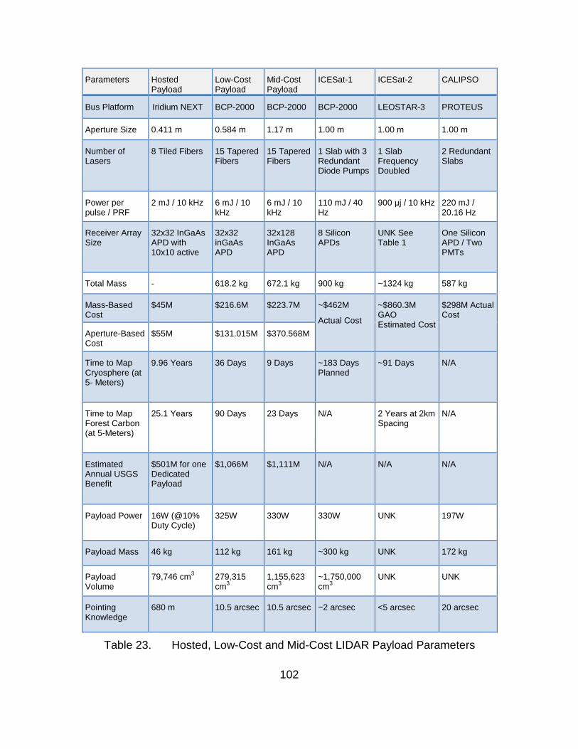
Parameters Hosted Payload
Low-Cost Payload
Mid-Cost Payload
ICESat-1 ICESat-2 CALIPSO
Bus Platform Iridium NEXT BCP-2000 BCP-2000 BCP-2000 LEOSTAR-3 PROTEUS
Aperture Size 0.411 m 0.584 m 1.17 m 1.00 m 1.00 m 1.00 m
Number of Lasers
8 Tiled Fibers 15 Tapered Fibers
15 Tapered Fibers
1 Slab with 3 Redundant Diode Pumps
1 Slab Frequency Doubled
2 Redundant Slabs
Power per pulse / PRF
2 mJ / 10 kHz 6 mJ / 10 kHz
6 mJ / 10 kHz
110 mJ / 40 Hz
900 μj / 10 kHz 220 mJ / 20.16 Hz
Receiver Array Size
32x32 InGaAs APD with 10x10 active
32x32 inGaAs APD
32x128 InGaAs APD
8 Silicon APDs
UNK See Table 1
One Silicon APD / Two PMTs
Total Mass - 618.2 kg 672.1 kg 900 kg ~1324 kg 587 kg
Mass-Based Cost
$45M $216.6M $223.7M ~$462M
Actual Cost
~$860.3M GAO Estimated Cost
$298M Actual Cost
Aperture-Based Cost
$55M $131.015M $370.568M
Time to Map Cryosphere (at 5- Meters)
9.96 Years 36 Days 9 Days ~183 Days Planned
~91 Days N/A
Time to Map Forest Carbon (at 5-Meters)
25.1 Years 90 Days 23 Days N/A 2 Years at 2km Spacing
N/A
Estimated Annual USGS Benefit
$501M for one Dedicated Payload
$1,066M $1,111M N/A N/A N/A
Payload Power 16W (@10% Duty Cycle)
325W 330W 330W UNK 197W
Payload Mass 46 kg 112 kg 161 kg ~300 kg UNK 172 kg
Payload Volume
79,746 cm3 279,315 cm3
1,155,623 cm3
~1,750,000 cm3
UNK UNK
Pointing Knowledge
680 m 10.5 arcsec 10.5 arcsec ~2 arcsec <5 arcsec 20 arcsec
Table 23. Hosted, Low-Cost and Mid-Cost LIDAR Payload Parameters
102
Based upon the cost modeling and estimated performance of these
designs, low-cost space-based LIDAR satellites have the ability to accomplish
the NASA and USGS mission while increasing performance over previous LIDAR
satellite designs. Technology advancements have allowed for increased area
collection rates in a smaller package and could benefit the pursuit of advanced
knowledge of the cryosphere, forest carbon stocks and the nation’s third
dimension. With multiple hosted payloads aboard Iridium or free flier payloads
paired with the BCP-2000 commercial bus, all three options have the ability to
exceed the performance characteristics of previous space-based LIDAR
systems. The area collection rates enabled by high efficiency, high pulse-power
and high PRF fiber lasers coupled with advanced InGaAs GmAPDs far exceed
that of the ICESat and CALIPSO missions. Recent advancements since the
design of ICESat-2 have the potential to reduce the cost of the mission. The
replacement of 532-nm planar waveguide lasers and detectors with more modern
1064-nm fiber lasers and GmAPD detector arrays could yield a lower cost
system with higher performance.
Preliminary analysis shows the potential for these new technologies to
outperform any previous space-based LIDAR mission. At $55M, the Iridium-
hosted solution is 1/16th the cost of ICESat-2 at roughly one-third its capability.
With three hosted payloads, the ICESat-2 mission could be accomplished at just
over 1/5th the cost. Two additional solutions are estimated at $216M and $370M,
providing over 3X and 10X the estimated capability of ICESat-2 at roughly one-
quarter and one-half the cost, respectively. These cost estimates and
performance numbers, however, are less mature than ICESat-2’s estimates and
should currently be viewed as options to be explored further for the future.
Nevertheless, these advancements and potential satellite designs enable a
potential future mission to satisfy both NASA and USGS objectives while
reducing the cost of such systems.
103

THIS PAGE INTENTIONALLY LEFT BLANK
104
LIST OF REFERENCES
Abdalati, W., Zwally, H. J., Bindschadler, R., Csatho, B., Farrell, S. L., Fricker, H. A., et al. (2010). The ICESat-2 laser altimetry mission. Proceedings of the IEEE, 98(5), 735–751.
Abshire, J. B. (2010). NASA’s space lidar measurements of earth and planetary surfaces. Frontiers in Optics 2010/Laser Science XXVI, pp. SMB1.
Andraschko, M., Antol, J., Baize, R., Horan, S., Neil, D., Rinsland, P., Zaiceva, R. (2012). The potential for hosted payloads at NASA. Aerospace Conference, 2012 IEEE, 1–12.
Andraschko, M., Antol, J., Horan, S., & Neil, D. (2011). Commercially hosted government payloads: Lessons from recent programs. Aerospace Conference, 2011 IEEE, 1–15.
Andrews, L. C., & Phillips, R. L. (2005). Laser beam propagation through random media. Bellingham, Wash: SPIE Press.
Applied Technology Associates. (2011). Fast steering mirror. Retrieved August 18, 2013, from http://www.aptec.com/fast_steering_mirror.html
Aull, B. F., Loomis, A. H., Young, D. J., Heinrichs, R. M., Felton, B. J., Daniels, P. J., et al. (2002). Geiger-mode avalanche photodiodes for three-dimensional imaging. Lincoln Laboratory Journal, 13(2), 335–349.
Becker, H. N., Farr, W. H., & Zhu, D. Q. (2007). Radiation response of emerging high gain, low noise detectors. Nuclear Science, IEEE Transactions on, 54(4), 1129–1135.
Brown, S. D., Blevins, D. D., & Schott, J. R. (2005). Time-gated topographic LIDAR scene simulation. Defense and Security, 342–353.
Burton, R. R. (2002). Elastic LADAR modeling for synthetic imaging applications (Doctoral dissertation). Rochester Institute of Technology, Rochester, NY.
Cavanaugh, J. F., et al. (2007). The Mercury Laser Altimeter Instrument for the MESSENGER Mission. Space Science Reviews, Vol. 131, 1–4, 451–479.
Cole, T. D. (1998). NEAR laser rangefinder: A tool for the mapping and topologic study of asteroid 433 eros. Johns Hopkins APL Technical Digest, 19(2), 143.
Coyle, D. B. (2005). Applications of fiber amplifier for space: Laser altimetry and mapping. Unpublished manuscript.
105
Dewberry. (2012). National enhanced elevation assessment. Fairfax, Virginia: United States Geological Survey.
Farrow, R. L., Kliner, D. A., Schrader, P. E., Hoops, A. A., Moore, S. W., Hadley, G. R., et al. (2006). High-peak-power (> 1.2 MW) pulsed fiber amplifier. Lasers and Applications in Science and Engineering, pp. 61020L–61020L-11.
Fox, B., Schneider, Z., Simmons-Potter, K., Thomes Jr, W., Meister, D., Bambha, R., et al. (2007). Gamma radiation effects in yb-doped optical fiber. Fiber Lasers IV: Technology, Systems, and Applications, Proc.SPIE, 6453, 645328.
Government Accountability Office. (2012). NASA Assessment of Selected Large-Scale Projects, GAO-13-276SP. Washington, D.C.: Government Accountability Office.
Guerra, L. (2008). Cost estimating module space systems engineering. Unpublished manuscript.
Harwood, W. (2009). Atlas 5 rocket launches NASA moon mission. Retrieved August 14, 2013, from http://news.cnet.com/8301-19514_3-10268241-239.html
Henson, R. (2008). Satellite observations to benefit science and society: Recommended missions for the next decade. Washington, DC: National Academies Press.
Huffington Post. (2011). A first: NASA MESSENGER spacecraft orbiting mercury. Retrieved August 14, 2013, from http://www.huffingtonpost.com/2011/03/18/nasa-MESSENGER-mercury_n_837503.html
Kichak, R. (2003). Independent GLAS anomaly review board executive summary. Greenbelt, Maryland: Goddard Space Flight Center.
Kim, S., Lee, I., & Kwon, Y. J. (2013). Simulation of a geiger-mode imaging LADAR system for performance assessment. Sensors, 13(7), 8461–8489.
Koechner, W., & Bass, M. (2003). Solid-state lasers: A graduate text. New York, New York: Springer.
Krainak, M. A., Anthony, W. Y., Yang, G., Li, S. X., & Sun, X. (2010). Photon-counting detectors for space-based laser receivers. Opto, pp. 760827-760827-9.
106
Leone, D. (2012). U.S. Air Force deferral of last DMSP upends plan for launching ICESat 2. Retrieved August 14, 2013, from http://www.spacenews.com/article/us-air-force-deferral-last-dmsp-upends-plan-launching-ICESat-2
Maiman, T. (1960). Stimulated optical radiation in ruby. Nature, 187(4736), 493–494.
Masursky, H., Colton, G. W., El-Baz, F., & Doyle, F. J. (1978). Apollo over the moon: A view from orbit. NASA Special Publication, 362.
McGill, M. (2011). Multiple altimeter beam experimental lidar (MABEL) first flights and initial results. Retrieved August 14, 2013, from http://atmospheres.gsfc.nasa.goc/science/slides.php?sclid=6
McGill, M., Markus, T., Scott, V. S., & Neumann, T. (2013). The multiple altimeter beam experimental lidar (MABEL): An airborne simulator for the ICESat-2 mission. Journal of Atmospheric and Oceanic Technology, 30(2), 345–352.
Nabuurs, G., & Masera, O. (2007). IPCC fourth assessment report: Climate change 2007, working group 3, forestry. Switzerland: Intergovernmental Panel on Climate Change.
NASA. (2007). Report from the ICESat-II workshop. Linthicum, Maryland: National Aeronautics and Space Administration.
NASA assessments of selected large-scale projects (2013). No. GAO-13-276SP. Washington, DC: Government Accountability Office.
NASA ICESat cryospheric sciences lab code 615. (2013). Retrieved September 30, 2013, from http://ICESat.gsfc.nasa.gov/ICESat/
NASA: ICESat-2. (2013). Retrieved September 30, 2013, from http://ICESat.gsfc.nasa.gov/ICESat2/
National Research Council (U.S.) Committee on Earth Science. (2007). Earth science and applications from space: National imperatives for the next decade and beyond. Washington, DC: National Academies Press.
National Snow and Ice Data Center. (2013). Quick facts on ice sheets. Retrieved September 30, 2013, from http://nsidc.org/cryosphere/quickfacts/icesheets.html
Neumann, G. (2001). Some aspects of processing extraterrestrial LIDAR data: Clementine, NEAR, MOLA. International Archives of Photogrammetry and Remote Sensing, Volume XXXIV-3/W4, pp. 73–80.
107
nLight. (2013). nLight high power lasers fiber-coupled. Retrieved September 30, 2013, from http://www.nlight.net/products/fiber-coupled/
Ramos-Izquierdo, L., Scott III, V. S., Connelly, J., Schmidt, S., Mamakos, W., Guzek, J., et al. (2009). Optical system design and integration of the lunar orbiter laser altimeter. Applied Optics, 48(16), 3035–3049.
Richard, J., Le Roy, Y., Thouvenot, E., & Escudier, P. (2008). Altimetry payload specification for Iridium NEXT. Bethesda, MD: Iridium Satellite LLC.
Riris, H., & Cavanaugh, J. F. (2010). Calibration document for the lunar orbiter laser altimeter (LOLA) instrument. Unpublished manuscript.
Riris, H., Sun, X., Cavanaugh, J. F., Jackson, G. B., Ramos-Izquierdo, L., Smith, D. E., et al. (2007). The lunar orbiter laser altimeter (LOLA) on NASA’s lunar reconnaissance orbiter (LRO) mission. Defense and Security Symposium, pp. 65550I-65550I-8.
Rosette, J., Field, C., Nelson, R., DeCola, P., & Cook, B. (2011). A new photon-counting lidar system for vegetation analysis. Proceedings of SilviLaser 2011, 11th International Conference on LiDAR Applications for Assessing Forest Ecosystems, University of Tasmania, Australia, 16–20 October 2011.
Sawruk, N. W., Stephen, M. A., Litvinovitch, S., Edelman, J. E., Albert, M. M., Edwards, R. E., et al. (2013). Space qualified laser transmitter for NASA’s ICESat-2 mission. Spie Lase, pp. 85990O-85990O-7.
Smith, D. E., & Zuber, M. T. LOLA fact sheet. Unpublished manuscript.
Smith, D. E., Zuber, M. T., Frey, H. V., Garvin, J. B., Head, J. W., Muhleman, D. O., et al. (2001). Mars orbiter laser altimeter: Experiment summary after the first year of global mapping of mars. Journal of Geophysical Research: Planets (1991–2012), 106(E10), 23689–23722.
Snyder, G. I. (2013). The benefits of improved national elevation data. Photogrammetric Engineering & Remote Sensing, 79(2), 105.
Sorensen T.C. and P.D. Spudis (2005), The Clementine Mission: A 10-year perspective. J. Earth System Sci, 114(6), 645–668.
Spudis, P. D. (1994). The Clementine mission: initial results from lunar mapping. Washington, DC: National Aeronautics and Space Administration.
Stahl, H. P., Henrichs, T., Luedtke, A., & West, M. (2012). Update on multivariable parametric cost models for ground and space telescopes. SPIE Astronomical Telescopes Instrumentation, pp. 844224-844224-6.
108
Starodoumov, A. (2008). Sequentially-Modulated Diode-Laser Seed-Pulse Generator. U.S. Patent No. US20090296759 A1. Washington, DC.
Tapos, F. M., Edinger, D. J., Hilby, T. R., Ni, M. S., Holmes, B. C., & Stubbs, D. M. (2005). High bandwidth fast steering mirror. Optics & Photonics 2005, pp. 587707-587707-14.
USA Today. (2003). Rocket carrying NASA satellites launched. Retrieved August 14, 2013, from http://usatoday30.usatoday.com/weather/news/2003-01-13-nasa-ICESat_x.htm
Wassom, S., Davidson, M., Newswander, T., Cook, J., Casper, Z., & Shelley, A. (2006). Fine steering mirror for smallsat pointing and stabilization. AIAA/USU Small Satellite Conference 2006. Logan, Utah.
Winker, D., Couch, R., & McCormick, P. (1996). An overview of LITE: NASA’s lidar in-space technology experiment. Proceedings of the IEEE, 84(2), 164–180.
Winker, D., Hunt, W., Hostetler, C. (2004). Status and performance of the CALIOP lidar. Laser Radar Techniques for Atmospheric Sensing, Proceedings of the SPIE, 5575, 8–15.
Winker, D. M., Hunt, W., & McGill M. (2007). Initial performance assessment of CALIOP. Geophys. Res. Lett., 34, L19803
The World Bank. (2013). Data: Land area. Retrieved September 2013, 2013, from http://data.worldbank.org/indicator/AG.LND.TOTL.K2
Yu, A. W., Harding, D. J., Abshire, J. B., Krainak, M. A., & Sun, X. (2011). Technologies development for the lidar surface topography (LIST) mission. 16th Coherent Laser Radar Conference. Long Beach, California.
Yu, A. W., Stephen, M. A., Li, S. X., Shaw, G. B., Seas, A., Dowdye, E., et al. (2010). Space laser transmitter development for ICESat-2 mission. Proceedings of the SPIE, pp. 757809-757809-11.
Yuan, P., Sudharsanan, R., Bai, X., Boisvert, J., McDonald, P., Labios, E., et al. (2011). Geiger-mode LADAR cameras. SPIE Defense, Security, and Sensing, pp. 803712-803712-10.
Zissis, G. J., & Wolfe, W. L. (1978). The infrared handbook. Ann Arbor, Michigan: Environmental Research Institute of Michigan.
Zuber, M. T., Smith, D. E., Solomon, S. C., Phillips R. J., Peale S. J., Head, J. W. III, … Harmon, J. K. (2008). Laser altimeter observations from MESSENGER’s first Mercury flyby. Science, 321, 77.
109

Zuber, M. T., Smith, D. E., Phillips, R. J., Solomon, S. C., Neumann, G. A., Hauck, S. A. II, … Yang, D. (2012). Topography of the northern hemisphere of Mercury from MESSENGER laser altimetry. Science, 336, 217.
110
INITIAL DISTRIBUTION LIST
1. Defense Technical Information Center Ft. Belvoir, Virginia 2. Dudley Knox Library Naval Postgraduate School Monterey, California
111


![· SHIM SACD Dire Straits rLove Over Gold] (Private Investigations) ' Clear Cygnus SACD ' , IRIDIUM , IRIDIUM , IRIDIUM 11.5 AWG , , PFA 3455R IRIDIUM Clear Cygnus , 5 Trigon Exxpert](https://img.pdfslide.us/doc/110x75/60d04de1d6909b691a4f38e7/shim-sacd-dire-straits-rlove-over-gold-private-investigations-clear-cygnus.jpg)