Embed Size (px)
Citation preview

NAVAL POSTGRADUATE
SCHOOL
MONTEREY, CALIFORNIA
THESIS
Approved for public release;distribution is unlimited
QUANTUM EFFICIENCY AS A FUNCTION OF TEMPERATURE IN METAL PHOTOCATHODES
by
Abdullah Kara
June 2013
Thesis Co-Advisors: Richard L. Swent John R. Harris

THIS PAGE INTENTIONALLY LEFT BLANK

i
REPORT DOCUMENTATION PAGE Form Approved OMB No. 0704–0188 Public reporting burden for this collection of information is estimated to average 1 hour per response, including the time for reviewing instruction, searching existing data sources, gathering and maintaining the data needed, and completing and reviewing the collection of information. Send comments regarding this burden estimate or any other aspect of this collection of information, including suggestions for reducing this burden, to Washington headquarters Services, Directorate for Information Operations and Reports, 1215 Jefferson Davis Highway, Suite 1204, Arlington, VA 22202–4302, and to the Office of Management and Budget, Paperwork Reduction Project (0704–0188) Washington DC 20503. 1. AGENCY USE ONLY (Leave blank)
2. REPORT DATE June 2013
3. REPORT TYPE AND DATES COVERED Master’s Thesis
4. TITLE AND SUBTITLE QUANTUM EFFICIENCY AS A FUNCTION OF TEMPERATURE IN METAL PHOTOCATHODES
5. FUNDING NUMBERS
6. AUTHOR(S) Abdullah Kara
7. PERFORMING ORGANIZATION NAME(S) AND ADDRESS(ES)Naval Postgraduate School Monterey, CA 93943–5000
8. PERFORMING ORGANIZATION REPORT NUMBER
9. SPONSORING /MONITORING AGENCY NAME(S) AND ADDRESS(ES)N/A
10. SPONSORING/MONITORING AGENCY REPORT NUMBER
11. SUPPLEMENTARY NOTES The views expressed in this thesis are those of the author and do not reflect the official policy or position of the Department of Defense or the U.S. Government. IRB Protocol number ____N/A____.
12a. DISTRIBUTION / AVAILABILITY STATEMENT Approved for public release;distribution is unlimited
12b. DISTRIBUTION CODE
13. ABSTRACT (maximum 200 words)
Photocathodes, in which light is used to extract electrons from materials by the photoelectric effect, are the principal electron sources for many linear accelerators and Free Electron Lasers (FELs). There is an increasing interest in the use of superconducting radiofrequency electron guns, which work at cryogenic temperatures, and therefore require photocathodes that work at cryogenic temperatures as well. The primary metric used to quantify photocathode performance is the cathode’s Quantum Efficiency (QE), which is the ratio between the number of incoming laser photons and outgoing electrons. The objective of this thesis is to measure the QE of metal photocathodes as a function of temperature. To accomplish this, a photocathode test stand capable of varying the temperature of metal samples from 80 K to 400 K was developed, and copper and niobium samples were tested using it. The QE of copper was found to vary by a factor of more than four over this temperature range, while the QE of niobium showed only slight temperature dependence.
14. SUBJECT TERMS Photocathodes, Niobium, Cryogenic Temperature, Quantum Efficiency.
15. NUMBER OF PAGES
85 16. PRICE CODE
17. SECURITY CLASSIFICATION OF REPORT
Unclassified
18. SECURITY CLASSIFICATION OF THIS PAGE
Unclassified
19. SECURITY CLASSIFICATION OF ABSTRACT
Unclassified
20. LIMITATION OF ABSTRACT
UU
NSN 7540–01–280–5500 Standard Form 298 (Rev. 2–89) Prescribed by ANSI Std. 239–18

ii
THIS PAGE INTENTIONALLY LEFT BLANK

iii
Approved for public release;distribution is unlimited
QUANTUM EFFICIENCY AS A FUNCTION OF TEMPERATURE IN METAL PHOTOCATHODES
Abdullah Kara Lieutenant Junior Grade, Turkish Navy
B.S., Turkish Naval Academy, 2007
Submitted in partial fulfillment of the requirements for the degree of
MASTER OF SCIENCE IN APPLIED PHYSICS
from the
NAVAL POSTGRADUATE SCHOOL June 2013
Author: Abdullah Kara
Approved by: Richard L. Swent, PhD Thesis Co-Advisor
John R. Harris, PhD Thesis Co-Advisor
Andres Larraza, PhD Chair, Department of Physics

iv
THIS PAGE INTENTIONALLY LEFT BLANK

v
ABSTRACT
Photocathodes, in which light is used to extract electrons from materials by the
photoelectric effect, are the principal electron sources for many linear
accelerators and Free Electron Lasers (FELs). There is an increasing interest in
the use of superconducting radiofrequency electron guns, which work at
cryogenic temperatures, and therefore require photocathodes that work at
cryogenic temperatures as well. The primary metric used to quantify
photocathode performance is the cathode’s Quantum Efficiency (QE), which is
the ratio between the number of incoming laser photons and outgoing electrons.
The objective of this thesis is to measure the QE of metal photocathodes as a
function of temperature. To accomplish this, a photocathode test stand capable
of varying the temperature of metal samples from 80 K to 400 K was developed,
and copper and niobium samples were tested using it. The QE of copper was
found to vary by a factor of more than four over this temperature range, while the
QE of niobium showed only slight temperature dependence.

vi
THIS PAGE INTENTIONALLY LEFT BLANK

vii
TABLE OF CONTENTS
I. INTRODUCTION ............................................................................................. 1 A. LASERS FOR THE NAVY ................................................................... 1 B. FREE ELECTRON LASERS ................................................................ 3
1. Components of an FEL ........................................................... 3 2. How FELs Work ....................................................................... 4
C. SRF LINEAR ACCELERATORS ......................................................... 5 D. SRF RESEARCH AT THE NAVAL POSTGRADUATE SCHOOL
(NPS) .................................................................................................... 7 E. ELECTRON SOURCES FOR FELS .................................................... 7
1. Electron Emission Process ..................................................... 7 2. Photocathodes ......................................................................... 8 3. Different Photocathode Types .............................................. 11
a. Metal Photocathodes .................................................. 12 b. Dispenser Photocathodes .......................................... 12 c. Semiconductor Photocathodes ................................. 12
II. QE TEST STAND ......................................................................................... 13 A. PHOTOCATHODE RESEARCH AT NPS .......................................... 13 B. INFORMATION ABOUT THE EQUIPMENT USED ........................... 14
1. Laser ....................................................................................... 14 a. Wavelength and Power ............................................... 15 b. Pulse Width ................................................................. 15 c. Optical Elements ......................................................... 16
2. Laser Power Meter ................................................................. 16 3. Cathode Stalk ......................................................................... 17
a. Cathode Cooling System ............................................ 18 b. Cathode Heating System ............................................ 19
4. Computer Software ................................................................ 20 a. Temperature Monitoring ............................................. 20 b. Automatic Laser Control ............................................ 21
5. Vacuum System ..................................................................... 23 6. High Voltage Unit ................................................................... 24 7. Electron Beam Measurement ................................................ 25
a. Bergoz Fast Current Transformer (FCT) ................... 25 b. Oscilloscope ................................................................ 26
C. FIRST-GENERATION TEST STAND ................................................. 27 D. THE TEMPERATURE-CONTROLLED TEST STAND ....................... 32
III. HOW THE QE EXPERIMENT WAS CONDUCTED ...................................... 35 A. UV WINDOW TRANSMISSION LOSS CALCULATION .................... 35 B. SPACE CHARGE LIMITED (SCL) REGIME IN TEMPERATURE-
CONTROLLED TEST STAND ........................................................... 36

viii
C. QE MEASUREMENTS ON TEMPERATURE-CONTROLLED TEST STAND ..................................................................................... 37 1. Cooling the Cathode Down to Cryogenic Temperatures .... 40 2. Creating a Stable Wave on the Oscilloscope ...................... 41 3. Data Derived from the Test Stand ........................................ 41
a. Cathode’s Instant Temperature ................................. 41 b. Vacuum Level of the Cathode’s Environment .......... 42 c. Averaged Laser Power ............................................... 44 d. Charge Per Pulse ........................................................ 44 e. The Peak Voltage Value of the Photoelectron
Pulse on the Oscilloscope ......................................... 45 4. Heating the Cathode up to 400K ........................................... 45
D. PROCESSING THE RAW DATA ....................................................... 46 1. Photon Number Calculation .................................................. 46 2. Electron Number Calculation ................................................ 47 3. Quantum Efficiency ............................................................... 48 4. Peak Current Calculation ...................................................... 48
E. ANALYZING THE DATA ................................................................... 49 1. Copper .................................................................................... 50 2. Niobium .................................................................................. 54
IV. RESULTS AND RECOMMENDATIONS FOR FUTURE WORK ................. 59 A. RESULTS FOR COPPER AND NIOBIUM ......................................... 59 B. RECOMMENDATIONS FOR FUTURE WORK .................................. 62
LIST OF REFERENCES .......................................................................................... 63
INITIAL DISTRIBUTION LIST ................................................................................. 67

ix
LIST OF FIGURES
Figure 1. Schematic diagram of an FEL. From [8]. .............................................. 3 Figure 2. Superconducting RF accelerating cavity. From [10]. ............................ 6 Figure 3. Photoemission. ................................................................................... 10 Figure 4. Photocathode QE versus lifetime of selected photocathodes under
actual operating conditions. From [19]. ............................................... 11 Figure 5. Continuum Minilite-II Nd:YAG laser. ................................................... 15 Figure 6. Laser power meter and sensor. .......................................................... 17 Figure 7. Cathode stalk with cooling and heating connections. ......................... 17 Figure 8. Cathode stalk holding niobium cathode sample and diodes. .............. 18 Figure 9. Cathode cooling system connected to LN tank. ................................. 19 Figure 10. Cathode stalk with heaters and variable autotransformer. .................. 20 Figure 11. Temperature monitoring programs. .................................................... 21 Figure 12. Laser system in aluminum enclosure. ................................................ 22 Figure 13. Laser remote control program. ........................................................... 23 Figure 14. Agilent Technologies turbo and ion vacuum pump systems. .............. 24 Figure 15. Glassman high voltage unit. ............................................................... 24 Figure 16. LeCroy high voltage probe. ................................................................ 25 Figure 17. Bergoz Fast Current Transformer (FCT). ........................................... 26 Figure 18. Agilent technologies oscilloscope. ...................................................... 26 Figure 19. Cooper cathode before and after the vinegar cleaning. ...................... 27 Figure 20. Varian Turbo-V 301-AG turbo pump. .................................................. 28 Figure 21. Schematic view of the first-generation test stand. .............................. 29 Figure 22. First-generation test stand. ................................................................. 29 Figure 23. First measurement of electron emission from the cathode. ................ 30 Figure 24. Laser power vs. peak current at 20 different voltages. ....................... 31 Figure 25. Schematic diagram of the temperature-controlled test stand. ............ 33 Figure 26. Temperature-controlled test stand. ..................................................... 34 Figure 27. UV window transmission loss test stand. ............................................ 35 Figure 28. Niobium and copper cathodes in their locations on cathode stalk,
respectively. ....................................................................................... 36 Figure 29. Laser power vs. Peak current for Nb SCL regime. ............................. 37 Figure 30. Laser beam spot on Nb cathode. ....................................................... 39 Figure 31. Temperature monitor at 80 K and Liquid level controller. ................... 40 Figure 32. Cathode temperature vs. vacuum level. ............................................. 42 Figure 33. Discolored areas on the cooper cathode due to the discharge. .......... 43 Figure 34. Photoelectron pulse on the screen with vertical boundaries. .............. 45 Figure 35. Image of temperature rise on computer software. .............................. 46 Figure 36. Schematic diagram of electron number calculation. ........................... 47 Figure 37. QE per cycle. ...................................................................................... 48 Figure 38. Results for copper at 85 K. ................................................................. 50 Figure 39. Results for copper at 150 K. ............................................................... 51 Figure 40. Results for copper at 200 K. ............................................................... 51

x
Figure 41. Results for copper at 250 K. ............................................................... 52 Figure 42. Results for copper at 300 K. ............................................................... 52 Figure 43. Results for copper at 350 K. ............................................................... 53 Figure 44. Results for copper at 400 K. ............................................................... 53 Figure 45. Dependence of QE on temperature for copper. .................................. 54 Figure 46. Results for niobium at 85 K. ............................................................... 55 Figure 47. Results for niobium at 150 K. ............................................................. 55 Figure 48. Results for niobium at 200 K. ............................................................. 56 Figure 49. Results for niobium at 250 K. ............................................................. 56 Figure 50. Results for niobium at 300 K. ............................................................. 57 Figure 51. Results for niobium at 350 K. ............................................................. 57 Figure 52. Results for niobium at 400 K. ............................................................. 58 Figure 53. Dependence of QE on temperature for niobium. ................................ 58

xi
LIST OF TABLES
Table 1. Typical photocathodes. ......................................................................... 9 Table 2. Quantum efficiency for copper and niobium illuminated with 266 nm
light. .................................................................................................... 61

xii
THIS PAGE INTENTIONALLY LEFT BLANK

xiii
LIST OF ACRONYMS AND ABBREVIATIONS
CW Continuous Wave
DF Deuterium Fluoride
DoD Department of Defense
FCT Fast Current Transformer
FEL Free Electron Laser
GaAs Gallium Arsenide
HEL High Energy Laser
LINAC Linear Accelerator
LN Liquid Nitrogen
ONR Office of Naval Research
QE Quantum Efficiency
SCL Space Charge Limit
SRF Superconducting Radiofrequency
WSMR White Sands Missile Range

xiv
THIS PAGE INTENTIONALLY LEFT BLANK

xv
ACKNOWLEDGMENTS
I would first like to thank my patient and grace-filled wife, Neslihan, who
endured my absence at home while I was doing my experiments at Sp044 for
long periods. I would also like to thank my thesis advisors, Dr. Richard L. Swent
and Dr. John R. Harris, who helped me with all their efforts whenever I needed
them, even across great distances. In addition, I want to express my gratitude to
Beam Physics Group members Wayne, Andrea, and Mark for their assistance in
preparing the test stands and in conducting the experiments. Finally, I also want
to say thank you to one more person, James Sears, who provided me with the
niobium samples for free. If I have done a good job, you all must know that I
accomplished it with your help. Thank you.

xvi
THIS PAGE INTENTIONALLY LEFT BLANK

1
I. INTRODUCTION
A. LASERS FOR THE NAVY
After the invention of the laser in 1960, the idea of using a laser as a
weapon quickly became of interest to the U.S. defense establishment, which
began investing in this technology [1]. In 1968, Ed Gerry achieved a 100-kW
output with a gas dynamic carbon dioxide laser, further accelerating interest in
laser weapons [2]. Different agencies pursued different technology approaches
based on their own military requirements. For the Navy, interest in high energy
laser (HEL) weapons was primarily driven by the need to defend surface
warships, especially carriers and their escort ships, against incoming anti-ship
missiles. Lasers were seen as a potential counter to this threat for several
reasons.
Since no ammunition is expended, the cost per engagement can be smaller with a laser than with other anti-missile systems.
Many laser systems have the potential to be very compact.
Laser weapons do not require the storage of explosive rounds, which can endanger the ship.
Laser energy travels with the speed of the light, while a typical bullet travels with an initial speed of Mach 3.5.
The range of the laser is defined by the horizon, while a bullet is limited by atmospheric drag and gravity.
The Navy’s HEL program soon demonstrated the ability to successfully
engage airborne targets with lasers. Much of this work was performed at the
White Sands Missile Range (WSMR), where a facility for testing high-power
lasers had been authorized by Congress in 1976 [3]. There, the SeaLite system,
which used an MW-class Deuterium Fluoride (DF) laser, shot down a BQM-34
drone aircraft in 1986. Three years later, the system shot down a Talos missile
simulating a supersonic cruise missile on a crossing trajectory at a tactically
meaningful range. Nevertheless, the system was not ideally suited for shipboard
applications due to its wavelength, which limited propagation through the

2
atmosphere. Additionally, it used toxic chemicals which were dangerous to the
crew and required frequent replenishment [4].
In parallel with chemical laser development, a new concept called the Free
Electron Laser (FEL) was suggested by J.M.J Madey in 1971 while he was at
Stanford University [5]. This concept did not use a chemical medium to obtain
laser light. Instead the new laser used a beam of free electrons. This concept
provided several potential advantages for the Navy:
FELs avoided use of toxic chemicals which introduce additional damage control and resupply problems for the warfighters.
With no conventional lasing medium, the problem of waste heat extraction was greatly simplified, providing the potential for very high-power operation.
Since it did not depend on quantum mechanical transitions between discrete energy status, as in other types of laser, it could be designed to operate at wavelengths that were favorable for energy transmission through the atmosphere [6].
Because of these features, the Navy believed that the FEL had significant
potential as a laser weapon, and the Navy officially initiated its FEL program in
1997 [7].
According to the Office of Naval Research (ONR):
The capability of having speed-of-light delivery for a wide range of missions and threats is a key element of future shipboard layered defense… This revolutionary technology allows for multiple payoffs for the warfighter. The ability to control the strength of the beam provides for graduated lethality, and the use of light vice an explosive munition, provides for lower per-engagement and life cycle costs. Not worrying about propulsion and working at the speed of light allows for precise engagement and the resulting low collateral damage. Speed-of-light engagement also allows for a rapid reaction to moving and/or swarming time critical targets [8].
Based on recent information, a new FEL weapon is envisioned for
shipboard use within ten years [9].

3
B. FREE ELECTRON LASERS
1. Components of an FEL
There are two types of FELs which are in most common use, the oscillator
configuration and the amplifier configuration. Coherent operation (lasing) requires
microbunching of the e-beam at the laser wavelength. Oscillators produce this
microbunching by using an optical cavity to feed spontaneous radiation back into
the undulator, while an amplifier uses an external source of light to generate the
microbunching.
The main parts of a typical FEL, as envisioned for use by the Navy and
shown in Figure 1, include an injector, a linear accelerator, an undulator, an
optical cavity, and a beam dump.
Figure 1. Schematic diagram of an FEL. From [8].
Electron beam production and initial acceleration occurs in the injector.
This section contains a cathode (electron source) inside an electron gun and may
also include a booster accelerator. Photocathodes are most commonly used as
the electron source and will be described in the next sections.
In the FELs envisioned by the Navy, the electron beam will be transferred
into a superconducting radiofrequency (SRF) linear accelerator (LINAC). This
device contains several metal cavities in which high-power electromagnetic fields
are used to accelerate electrons up to about 100 MeV.

4
After electrons are accelerated by the LINAC, they enter the undulator.
The undulator contains a series of magnets which supply an alternating magnetic
field that moves the electrons back and forth. This wiggling causes photon
emission from the relativistic electrons.
The undulator is typically located within an optical cavity. In an oscillator-
type FEL, the optical cavity comprises two mirrors located at the ends of the
cavity. One of the mirrors is partially transmissive, while the other one is fully
reflective. These mirrors provide the feedback needed for the FEL oscillator to
start up from noise, while still allowing some of the optical power in the cavity to
exit through the partially transmissive mirror and to be sent through the beam
director and on to the target.
Amplifier-type FELs, on the other hand, use a seed laser instead of
mirrors to produce gain.
Only a small fraction of the electron beam power will be converted to laser
light. Recycling the rest of the electron beam energy will increase the FEL’s
overall efficiency. In order to achieve this, a large quantity of the electron beam
power must be reclaimed. To do this, the electron beam exiting the undulator is
directed by magnets to re-enter the accelerator. However, this time they will enter
with a 180-degree phase shift. This phase shift causes them to release their
energy to the RF field and slow down. After as much energy as possible is
removed from the electron beam, it will be sent to the beam dump. The beam
dump absorbs the remaining beam energy, in the process generating heat and x-
rays, which requires that the beam dump be shielded and cooled.
2. How FELs Work
An FEL produces laser radiation using the energy from a relativistic beam
of electrons. In FELs, electron beams are used as the lasing medium, while in
conventional lasers, a gas, liquid, or solid is utilized for this purpose. This
accounts for many of the differences between conventional lasers and FELs. For
example, in conventional lasers waste heat must be extracted through the lasing

5
medium, while in an FEL the waste heat is removed from the lasing region at
nearly the speed of light as a part of the electron beam. In addition, the lasing
medium in a conventional laser limits it to specific wavelengths, while the FEL
offers both “designability” (to select the band before the FEL is built) and
“tunability” (to adjust the wavelength within that band after the FEL is built).
After the electrons are produced and accelerated to relativistic speeds, they are
directed to enter the undulator. The undulator produces an alternating magnetic
field which creates a strong Lorentz force that deflects the electron beam back
and forth, causing the beam to radiate electromagnetic energy. Creating an
optical field that interacts with the electron beam causes bunching of the
electrons at the optical wavelength. The FEL wavelength is given by
2
21
2 2u K
, (1.1)
where is the light wavelength, u is the undulator wavelength, and is the
Lorentz factor. The undulator parameter is given by22
rms ueBK
mc
, and depends on
the magnetic field B, undulator period, electron charge e, speed of light c, and
electron mass m [9].
Once the electrons have become microbunched at the optical wavelength,
they are able to coherently radiate at that wavelength. The radiation power then
scales with the square of the number of electrons, rather than with the number of
electrons, as is the case for non-coherent (spontaneous) emission. The radiation
process by which the electrons give up a significant fraction of their energy to the
optical field is therefore more efficient, increasing the power in this field and
therefore generating gain.
C. SRF LINEAR ACCELERATORS
Radio frequency linear accelerators are widely used for acceleration of
electron beams. These structures use high-frequency, high-power
electromagnetic fields synchronized with the electron beam, which enables the

6
electrons to gain energy from the fields, allowing them to gain hundreds or
thousands of MeV in some machines. It is from this energy that an FEL is able to
generate laser light.
Traditional accelerators are made of copper and can work at room
temperature, with cooling provided by water serving to remove heat deposited in
the copper due to the electrical power loss. However, a new type of linear
accelerator has been developed over the past few decades, which uses
superconducting materials such as niobium instead of copper (Figure 2). These
structures are very efficient due to their very low electrical losses and are well-
suited to continuous wave (CW) operation. One disadvantage of these structures
is that they must be operated at cryogenic temperatures in order to stay
superconducting.
Despite this disadvantage, SRF linear accelerators are the structures of
choice for future Navy FELs due to their very low electrical losses, which is
essential to efficiently transfer energy from the decelerating beam to the
accelerating beam in “energy-recovery linac” configurations such as the one
shown in Figure 1.
Figure 2. Superconducting RF accelerating cavity. From [10].

7
D. SRF RESEARCH AT THE NAVAL POSTGRADUATE SCHOOL (NPS)
With the increasing interest by the Navy in FELs as future weapon
systems for shipboard use, the FEL research group at the NPS was expanded to
include an experimental team, the NPS Beam Physics Laboratory, which is
focused on the development of accelerator technologies needed for these
systems. SRF technology has been of particular interest. This included SRF
electron guns; while SRF accelerators have been in use for several decades,
SRF electron guns are a relatively new development and not a mature
technology.
The NPS Beam Physics Lab and its Boeing and Niowave collaborators
were successful in building and testing the first purpose-built SRF electron gun in
the United States. During initial testing, the cavity demonstrated acceptable
beam parameters in terms of bunch charge and emittance, and it showed
promise in progressing to the full design gradient [11]. Complete details of the
design and commissioning of the gun were reported in [12]. Although some minor
problems were encountered during the testing, such as the failure of the NbTi
solenoid to superconduct, there were not any serious problems, such as severe
multipacting or cavity quenching. By the end of the experiment the measured
performance was found to be sufficient for NPS’s planned FEL experiments in
the infrared [12]. This successful demonstration of a new gun design only 24
months after concept represented a remarkably short development period
compared to other electron gun projects.
E. ELECTRON SOURCES FOR FELS
1. Electron Emission Process
Electrons are utilized to create the laser beam in FELs, but first we need
to produce the electrons themselves. Under normal conditions, electrons stay
inside solid matter because it is energetically favorable for them to do so. So to
generate free electrons, we must either give them enough extra energy to
overcome the energy barrier at the surface of the material, or we must change

8
the potential barrier. The amount of energy needed to extract electrons from the
material is called the work function, and cathodes are classified according to how
this energy is imparted:
“Thermionic emission” occurs when the cathode material is heated
sufficiently so that some of the electrons inside the material gain enough kinetic
energy to overcome the potential barrier. This type of emission happens in
thermionic cathodes, which are widely used in microwave radar tubes.
“Secondary emission” occurs when a primary electron beam collides with
a material and transfers some of its energy to the electrons in that material,
giving these “secondary electrons” enough energy to overcome the potential
barrier. Secondary emission plays an important role in the discharge process
such as vacuum surface flashover and multipactor.
“Field emission” occurs when a very strong electric field is applied to the
surface of the cathode material, causing the potential barrier at the surface to be
distorted, reducing its effective width and allowing electrons to tunnel through it to
the vacuum level and become free. Field emission cathodes are being studied by
some researchers for use in FELs of the type being considered by the Navy.
An extreme case of modifying the potential barrier is the “plasma
cathode.” Plasma containing positive ions and electrons can be produced
through various discharge processes, and by applying a strong electric field, the
electrons can be extracted. Plasma cathodes are capable of producing very large
currents, and therefore have potential use in high-power microwave sources.
However, they are generally limited by the expansion of the plasma, an effect
recently studied at NPS by A. Yilmaz, who conducted thesis research on a
flashboard plasma cathode test stand [13].
2. Photocathodes
The focus of this thesis, however, is the photocathode, which is the most
common source of electrons in FELs.

9
Photoemission, or the photoelectric effect, was first observed by Heinrich
Hertz in 1887 and later explained by Albert Einstein in terms of quantum
mechanics in 1921, for which he won the Nobel Prize [14], [15].
In photoemission, electrons are produced by light striking the cathode
surface. According to photoelectric emission theory, if we want to remove
electrons from the surface of a metal using this light, then the photons must
impart an amount of energy to the electrons so that they exceed the work
function. This is the minimum energy required to remove an electron from a
solid’s surface to a point directly outside the surface. In other words, this is the
energy required to carry an electron from the Fermi level to the vacuum level. If
the incident photon energy coming directly to the surface of the solid is less than
the work function of the solid, then no electrons are emitted. If the incident
photon energy is higher than the work function, the extra energy goes into kinetic
energy of the freed electron.
The photoelectric work function is:
Φ h (1.2)
where “h “ is the Planck’s constant and “ “ is the minimum (threshold) photon
frequency required to produce photoelectrons. The work function depends on the
type of cathode material used. Table 1 shows the work functions for typical
photocathode materials used in FELs.
Cathode Material Work Function (eV)
1 Magnesium (Mg) 3.6 [17]
2 Lead (Pb) 4.0 [16]
3 Niobium (Nb) 4.38 [16]
4 Copper (Cu) 4.6 [16]
5 CsBr:Cu (Coated) ~ 2.5 [18]
6 CsBr:Nb (Coated) ~ 2.5 [18]
Table 1. Typical photocathodes.

10
Photocathodes are the most common electron sources used in FELs,
because short-pulse lasers are available which turn the electron emission on and
off very quickly, producing very short, high-quality electron pulses.
Figure 3. Photoemission.
After electrons are produced from the cathode, they need to be
accelerated by a superconducting gun, for example, in order to make an electron
beam. So both gun and cathode must be congruous with each other. For
example, superconducting guns are operated at cold temperatures, in contrast to
thermionic cathodes which work at high temperatures. Because of this,
photocathodes are the most appropriate electron sources for this type of gun.
It is essential to define the effectiveness of a cathode sample used as a
part of a vacuum electronic device; Quantum Efficiency (QE) is used as one such
criterion. The QE is the ratio between the number of emitted electrons and the
number of incident photons.
#
#
electronsQE
photons (1.3)
Different cathode samples have different QE values. Scientists desire to
acquire robust, long lived, and high QE value cathodes. However, according to
some studies [19], this situation does not seem to happen easily. Cathodes with

11
long lifetimes usually have low QEs, and vice versa; this trade-off between QE
and long lifetime is shown in Figure 4.
Figure 4. Photocathode QE versus lifetime of selected photocathodes under actual operating conditions. From [19].
3. Different Photocathode Types
Scientists have performed many experiments on photocathodes. They
started their experiments with bare metals, such as copper, magnesium, etc. As
time went by, more complicated materials were used because of the need for
obtaining high QE values.

12
a. Metal Photocathodes
These were the initial electron sources used by scientists as
photocathodes. They are prompt, rugged, and have long lifetimes, but require
higher intensity lasers as their QEs are on the order of 0.001 – 0.01% [20].
b. Dispenser Photocathodes
By depositing other materials, such as a partial monolayer of
cesium, on the surface of a metal photocathode, its work function can be
reduced, and its QE can be increased. However, these layers are often fragile
and require replenishment. In order to do this in situ, a compact configuration
known as a dispenser photocathode has recently been introduced. This is an
adaptation of the dispenser cathode geometry used in thermionic cathodes. The
dispenser photocathode has a reservoir of low work function material which
partially coats the cathode surface to improve its QE. Primarily these
configurations were developed at the University of Maryland, with some testing
done recently at NPS [21], [22].
c. Semiconductor Photocathodes
Semiconductor photocathodes such as Gallium Arsenide (GaAs)
require much lower-intensity drive lasers and can produce polarized electron
bunches, but they generally require better vacuum conditions because they are
more fragile [23]. Direct band-gap p-type semiconductor photocathodes, such as
alkali antimonides and alkali tellurides, are the primary electron sources for many
accelerators, and they are now in operation at the Thomas Jefferson National
Accelerator Facility. They have high QE values on the order of 30% and are
operable at longer wavelengths. However, they are chemically reactive, easily
poisoned, and easily damaged by ion back bombardment [24].
13
II. QE TEST STAND
A. PHOTOCATHODE RESEARCH AT NPS
Previous cathode research projects have been performed at NPS with the
aim of developing better electron sources than the ones currently used in
accelerators and microwave sources. These projects investigated explosive
emission [25], flashboard plasma [13], and cesium coated cathodes [21].
This research thesis is mainly focused on metal photocathode operation at
both cryogenic and elevated temperatures. There has been much prior research
on the measurement of QE of metal cathodes [26], [27], [28]. However, most of
these experiments studied cathodes at or above room temperature, and we are
not aware of any research on the dependence of photoelectron emission on the
temperature of metal cathodes at cryogenic temperatures. As mentioned in the
previous chapter, SRF electron guns work at very cold temperatures. In these
systems, the cathode will stay in a cryogenic environment during the electron
production process, so it is important to understand how the cathode will behave
in this environment. In particular, we wanted to determine whether there is a
temperature effect on the number of electrons produced for a given amount of
incident light. To do this, we expose the cathode to light while it is at cryogenic
and high temperature conditions, apply an electric field to extract the
photoelectrons produced, and record the required data to calculate QE.
For a cathode material, we initially used copper, because it is abundant
and cheap. Initial testing with copper was performed in a test stand without the
ability to alter the cathode temperature, which allowed us to verify laser
performance and test procedures. With the help of these results, a newly
designed test stand and cathode stalk with the ability to control the cathode
temperature were tested to verify operations. This was again done with a copper
cathode first so as not to damage the main niobium sample. Later on, niobium,

14
which is more expensive and rare, was tested within the same test stand and
under similar conditions.
The light source used in this research was a Continuum Minilite Nd:YAG
laser, which produces a 5 ns long pulse of 266 nm UV light [29]. When the laser
light is directed onto the cathode sample, the light excites the electrons over the
surface potential barrier. A positive high voltage was applied to part of the
vacuum system to behave as an anode. The electrons emitted from the cathode
moved to the anode, causing a current flow along the cathode stalk towards the
cathode. A Bergoz Fast Current Transformer (FCT-016–20:1-WB-H) was
mounted around the cathode stalk for monitoring this electron flow on the
cathode stalk, and therefore served as a measure of emitted current.
The components used to assemble the test stands, as well as the design
and operation of the preliminary and the temperature-controlled test stands, are
discussed in the remainder of this chapter.
B. INFORMATION ABOUT THE EQUIPMENT USED
First of all to do this research, we needed to build a test stand which
ultimately included nearly a dozen pieces of equipment, distributed among
several main subsystems. This equipment is discussed here.
1. Laser
The laser is one of the key elements in our test stand. In this test stand,
electrons are emitted by photoemission, requiring that we shine light onto the
cathode’s surface. In order to do this, we used a Continuum Minilite-II Nd:YAG
laser. It is a Class 4 laser, which is the most dangerous laser type. Special safety
goggles were worn to protect our eyes from the hazard of the laser light.

15
Figure 5. Continuum Minilite-II Nd:YAG laser.
a. Wavelength and Power
The laser produces light in four different wavelengths between the
ultraviolet (UV) and infrared (IR). These are 266, 355, 532, and 1064 nm. To
select the best wavelength to shine on the cathode, we must find out the work
function of the cathode materials. It is essential that the energy of the photons
used exceeds this value to allow photoemission. As mentioned previously, the
work function for niobium is 4.38 eV, and for Copper it is 4.6 eV. Of the
wavelengths our laser can produce, only 266 nm satisfies this requirement, and
so only 266 nm UV light is applied in our experiments [16].
The laser’s power also varies with the wavelength. At the 266 nm
wavelength, it can produce up to 40 mW.
b. Pulse Width
Another principle specification of the laser is its pulse width. The
Minilite produces a pulse of laser light which is 3 to 7 ns in width, depending on

16
the wavelength used. For 266 nm wavelength, its pulse width value is between
3–5 ns.
c. Optical Elements
In order to obtain pure UV light and control the laser power
remotely, we mounted some optical elements, including some that were remote
controlled, between the laser and the cathode. We placed a green light filter to
block the green/visible light which was not fully converted to UV inside the laser.
Another optical element was needed to balance the requirement for relatively low
power at the cathode and relatively high power at our power meter. So, we
inserted a 30% transmissive and 70% reflective beam splitter into the optical
beamline. We also located a shutter blocking the laser beam and a remote-
controlled polarizer to increase or decrease the laser power from outside the
laser enclosure.
2. Laser Power Meter
We used a Coherent FieldMax-II TOP laser power and energy meter
connected to a PM10 Air-Cooled Thermopile Sensor, which could detect
wavelengths between 190 nm and 11000 nm. The power meter can detect laser
powers between 10 µW and 30 kW with a thermopile sensor. However, during
testing, we required that the laser power at the sensor was 5 mW because the
sensor was not rated for lower power, and initial testing at lower incident power
showed that the sensor’s response was nonlinear outside its specified range.

17
Figure 6. Laser power meter and sensor.
3. Cathode Stalk
As indicated, our aim is to measure QE under both cryogenic and high
temperature conditions. To achieve this goal, we must cool and heat the cathode
material; therefore, we designed and manufactured a new cathode stalk that
holds the cathode and includes cooling and heating systems to add or remove
heat from the cathode. Solid bulk copper was chosen for this purpose (Figure 7)
because it is a very good conductor of heat.
Figure 7. Cathode stalk with cooling and heating connections.

18
The cathode sample’s diameter was 19 mm with a thickness of 3 mm.
Before we placed the cathode samples in their locations on the cathode stalk,
they were cleaned by using alcohol and lint free wipes.
For monitoring the cathode temperature, we used two temperature-
sensing diodes of the type commonly used in cryogenic research. These were
located at the very end of the cathode stalk, with one placed on either side of the
cathode sample. The diode behind the cathode is a LakeShore DT-670-CU-HT,
which withstands temperatures up to 500 K, and the diode in front of the cathode
is a LakeShore DT-670-SD, which withstands temperatures up to 400 K. The
diode behind the cathode is in a well and is pushed against the back of the
cathode with a spring. The diode on the front is pushed against the cathode by
the bent edge of the washer visible in Figure 8.
Figure 8. Cathode stalk holding niobium cathode sample and diodes.
a. Cathode Cooling System
To take data from the test stand at cryogenic temperatures, we
cooled the cathode to 80 K using the liquid nitrogen (LN) cathode cooling system
previously built and tested by LT A. Baxter [30]. A fill-pot, shown in Figure 9, is
used as a LN phase separator to provide more consistent LN flow to the cathode

19
stalk cooling coil by eliminating or reducing gas bubbles. This allows the system
to cool faster and stay cold more efficiently. The fill-pot is connected directly to
the dewar through a solenoid valve controlled by an AMI Model 186 Liquid Level
Controller. There is a sensor inside the fill-pot to determine the level of the liquid.
Figure 9. Cathode cooling system connected to LN tank.
b. Cathode Heating System
For heating the cathode up to 400 K, two cartridge heaters were
placed into holes drilled in the cathode stalk. The heaters were connected to a
variable autotransformer to supply variable voltage for heating the cathode. Both
heaters and the autotransformer are shown in Figure 10.

20
Figure 10. Cathode stalk with heaters and variable autotransformer.
4. Computer Software
We set up some useful software to control and monitor the heating and
laser systems, which simplified and automated many of the required
measurements.
a. Temperature Monitoring
Two cryogenic diodes are located around the cathode to monitor
the exact cathode temperature. Both diodes are connected to a computer via a
LakeShore 218 temperature monitor, where we can see the increase and
decrease of temperature. To do this easily, a LabView program written by Prof.
Swent of the NPS Department of Physics, reads both temperature values and
displays them on a chart, which makes it easier for us to recognize the general
trend of the temperature, and saves this data to a file. The front panel display
and representative data from this program are shown in Figure 11.

21
Figure 11. Temperature monitoring programs.
b. Automatic Laser Control
We can control the laser beam by manually adjusting the laser
power using a control lever on the laser head. However, for most of this work the
laser system was inside an aluminum enclosure, which surrounded the high-
voltage end of the test stand as well as the laser head, to protect us not only from
the hazard of UV light but also from the high voltage (Figure 12).

22
Figure 12. Laser system in aluminum enclosure.
To avoid having to open the enclosure frequently, we connected
the laser beam control elements, such as the beam polarizer and shutter, to the
same computer used for temperature logging, and another LabView program
was written for controlling them remotely (Figure 13).

23
Figure 13. Laser remote control program.
5. Vacuum System
After the electrons leave from the cathode surface, they proceed towards
the positively charged vacuum pipe, which serves as the anode. During this
period they must move without hitting any molecules of air. Before we started
assembling the test stand, every piece of the vacuum system was cleaned
thoroughly with lint free napkins and alcohol to remove any contamination that
might prevent the vacuum pressure from reaching satisfactory levels. We then
connected two vacuum pumps onto the test set to remove the air.
The first pump was an Agilent model TPS-Compact 9698222 turbo pump,
which was able to achieve a base pressure of about 610 Torr. An ion pump was
added, and the vacuum level dropped down to 910 Torr (Figure 14). Vacuum
pressure inside the test stands was a function of cathode temperature, and in
practice the rate of cathode heating had to be limited to a level that did not cause
the vacuum pressure to spike.

24
Figure 14. Agilent Technologies turbo and ion vacuum pump systems.
6. High Voltage Unit
In order to collect and direct the emitted electrons, there must be a
positively charged piece called the anode. We connected a Glassman High
Voltage unit which supplies a positive direct current (DC) voltage of up to10 kV to
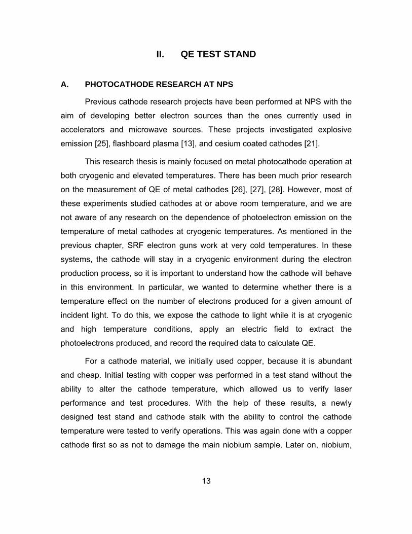
the vacuum spool piece in front of the cathode (Figure 15). A LeCroy high
voltage probe was attached to the vacuum spool piece with the voltage to
confirm the exact voltage value (Figure 16). Electrical insulation was provided by
ceramic breaks.
Figure 15. Glassman high voltage unit.
25
Figure 16. LeCroy high voltage probe.
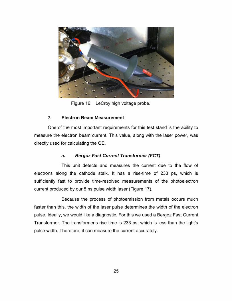
7. Electron Beam Measurement
One of the most important requirements for this test stand is the ability to
measure the electron beam current. This value, along with the laser power, was
directly used for calculating the QE.
a. Bergoz Fast Current Transformer (FCT)
This unit detects and measures the current due to the flow of
electrons along the cathode stalk. It has a rise-time of 233 ps, which is
sufficiently fast to provide time-resolved measurements of the photoelectron
current produced by our 5 ns pulse width laser (Figure 17).
Because the process of photoemission from metals occurs much
faster than this, the width of the laser pulse determines the width of the electron
pulse. Ideally, we would like a diagnostic. For this we used a Bergoz Fast Current
Transformer. The transformer’s rise time is 233 ps, which is less than the light’s
pulse width. Therefore, it can measure the current accurately.

26
Figure 17. Bergoz Fast Current Transformer (FCT).
b. Oscilloscope
The transformer was connected to an Agilent Technologies
DSO7054B digital storage oscilloscope where we read and recorded the data.
This oscilloscope also provides a capability to integrate the measured current to
determine the amount of charge extracted from the cathode. This oscilloscope,
along with a typical electron current and charge measurement, is shown in Figure
18.
Figure 18. Agilent technologies oscilloscope.

27
C. FIRST-GENERATION TEST STAND
At the beginning of this thesis research, a first-generation test stand was
built which did not have the ability to control the cathode temperature or to test
different cathode materials. Our aim with this test stand was to shake down the
laser, high voltage supply, and associated equipment, and to gain experience
using these systems to take photoemission measurements.
For the cathode in this test stand, we used a high-current vacuum
feedthrough, which was already on hand. This feedthrough consisted of a solid
copper rod mounted in a 342 " conflat flange and was electrically isolated from
the flange by a ceramic insulator (Figure 19). The copper rod had a flat surface,
which was convenient for use as the emitting surface. However, the copper had
been exposed to air and moisture for a long time. To remove its surface oxidation
layer, the copper was dipped into a vinegar-salt mixture to clean the surface.
After ten minutes a clear difference at the cathode’s surface was seen, as shown
in Figure 10.
Figure 19. Cooper cathode before and after the vinegar cleaning.
After deciding on the cathode material, we started assembling the test set.
Each component of the test set was cleaned meticulously with alcohol and lint
free wipes to achieve a lower vacuum level, which was desired for getting good
experimental results.

28
We should also mention another pump that was used in our initial test
stand. It was a Varian Turbo-V 301-AG turbo pump, which was capable of
reducing the vacuum inside the test stand down to about 710 Torr (Figure 20).
Figure 20. Varian Turbo-V 301-AG turbo pump.
High voltage from the Glassman power supply was applied to a vacuum
spool piece to serve as an anode and attract the emitted electrons from the
cathode. This spool was electrically isolated from the rest of the test stand with
two ceramic breaks. One of these breaks was mounted coaxially with the
cathode rod, and a Bergoz FCT was placed around it to measure the emitted
current. The UV window where the laser beam enters the vacuum chamber was
located at the end of the system near the vacuum pumping part. There was
concern that the emitted electrons might move directly towards the UV window’s
inside surface and gather there, charging up the glass and causing a discharge
leading to breakage or shattering. As a result, the window was placed as far
downstream as possible and in a region of the test stand that was at the cathode,

29
rather than the anode, potential. The entire test stand was enclosed in a
Plexiglas box to protect against the high voltage hazard (Figure 21).
Figure 21. Schematic view of the first-generation test stand.
Figure 22. First-generation test stand.
Later we started using the test stand. At first we gained experience on
using, controlling, and adjusting the laser beam. When we achieved a certain
level of expertise with this, we pumped out the air from the chamber, applied high
voltage, made the connection to the oscilloscope, and directed the laser onto the

30
copper cathode, producing our first photoelectrons. Our initial electron beam
measurement taken on a Tektronix TDS 714L oscilloscope is shown in Figure 23.
Figure 23. First measurement of electron emission from the cathode.
As expected, we observed that the electron current detected by the
Bergoz FCT depended primarily on laser power for low laser power values.
Electron current flow from a photocathode can be expressed by
0.124
PI QE
, (3.1)
where I is the electron current (in mA), is the laser wavelength (in nm), P is
the applied laser power (in mW), and QE is the quantum efficiency (in percent)
[29]. As we see from the equation, the laser power (P) and electron current are
proportional to each other; they increase or decrease together linearly to hold the
QE constant.
However, over a certain laser power level, the increase in current for a
given increase in laser power (dI
dP) will decrease. This is not due to a change in
QE, but rather due to space charge, an accumulation of charge in front of the
cathode which serves to shield the cathode from the electric field produced by
the anode and, therefore, to prevent the emission of additional electrons. Figure
24 shows experimental data obtained with the preliminary test stand. This data,
plotted as peak current vs. laser power incident on the cathode for 20 different

31
voltage values from 0.5 kV to 20 kV, clearly shows both linear (emission-limited)
region and the nonlinear (space-charge limited) regions.
Figure 24. Laser power vs. peak current at 20 different voltages.
This data shows that the “space-charge limited” (SCL) regime started
when the laser power reached around 5 mW. Because the objective of this
project was to measure QE, it was essential to stay below the value at which the
current was limited by space charge. And while the space-charge limited current
depends on geometry, the temperature-controlled test stand was designed with a
similar geometry, and therefore we expected to see similar behavior
After having gained experience with these issues, we were ready to start
assembling our new cryogenic test stand.

32
D. THE TEMPERATURE-CONTROLLED TEST STAND
We were now ready to initiate our new test stand and obtain new results.
This time our goal was to include all the instruments which were not used on the
previous test stand. In particular, our goal was also to add the ability to heat or
cool the cathode.
In addition to incorporating the components discussed previously, the
temperature-controlled test stand used larger-diameter vacuum pipes, providing
improved pumping capacity. All the vacuum pieces were cleaned with alcohol
and lint free wipes before assembly. The cathode stalk was the first part, which
was located inside the vacuum chamber. Later, electrical connections for the
temperature measuring diodes and heaters were made, and next the turbo and
ion pumps were attached. The high voltage unit was attached directly to the front
most vacuum element. Then, the cathode cooling system was connected to the
whole test stand. Finally, an aluminum enclosure box protecting us from the high
voltage and laser hazards was placed around the test stand.
Before we started conducting the experiment, we turned on the vacuum
pumps. Initially the turbo pump was operated until the vacuum level inside the
chamber dropped -610 Torr. Then, we turned on the ion pump to reduce the level
more. Before we started taking data from the test stand, the vacuum level
reached -710 - -810 Torr at room temperature conditions.
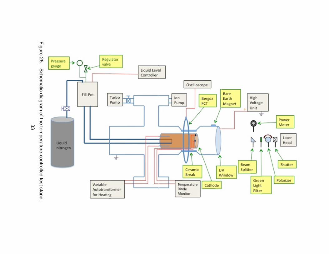
A schematic of the assembled test stand is shown in Figure 25, and a
photograph of the test stand’s control station is shown in Figure 26.
33
Figure 25.
Schem
atic diagram of the tem
perature-controlled test stand.
Vanable Autotransformer for Heating

34
Figure 26. Temperature-controlled test stand.
When we finished building the test stand, we were ready to shine the laser
on the cathode and make photoelectrons. This time, however, we also got the
cooling and heating systems ready. For initial testing, a copper cathode sample
had been inserted into the cathode stalk. We illuminated the cathode with the
laser and observed the electron beam current on the oscilloscope, producing the
oscilloscope traces of beam current vs. time. We were now curious to see
whether there was a significant variation in the beam current when we changed
the cathode temperature.
At first the cathode was heated gradually up to 400 K by applying current
to the heaters with the variable autotransformer. We observed a significant
increase in the beam current displayed on the oscilloscope screen. Next, we
cooled the cathode down to 80 K by using LN. It was seen that there was also a
significant reduction in the beam current compared to the signal seen at room
temperature. These changes were much greater than we had expected. Thus,
this scene upgraded our enthusiasm for achieving better results.

35
III. HOW THE QE EXPERIMENT WAS CONDUCTED
A. UV WINDOW TRANSMISSION LOSS CALCULATION
As expressed in Chapter I, we used UV laser light where the wavelength
is 266 nm because of the work function of the copper and niobium. We mounted
a UV window in front of the cathode stalk on the vacuum chamber, where the
laser light entered. For actual calculations, we had to determine the most
accurate laser power inside the vacuum chamber, and this required measuring
the UV glass transmission loss.
A basic test stand was designed and utilized for this purpose. Our aims
were to define the laser power just before and after the UV window and to
calculate the transmission ratio. The laser light and UV window were aligned on
the same plane.
Figure 27. UV window transmission loss test stand.
This calibration process was conducted in two steps. In the first step the
power meter was placed just in front of the UV window, and the laser power was
measured and recorded. In the second step the laser power meter was placed
immediately behind the UV window and the laser power was measured and

36
recorded. These values were used to find the fraction of laser power which was
not transmitted through the window,
2 1
1
P - PNT =
P, (3.1)
where 1P is the power upstream of the window, and 2P is the power downstream
from the window. Finally we used equation 3.2 to obtain the transmission
coefficient “T.”
T =1- NT (3.2)
This measurement was repeated 19 times, with the power meter reversed
between each measurement. Our average transmission coefficient found in this
way was 0.922 ± 0.00.
B. SPACE CHARGE LIMITED (SCL) REGIME IN TEMPERATURE-CONTROLLED TEST STAND
Achieving accurate QE results requires operating below the SCL. The
SCL current depends on the geometry of the system and on the anode-cathode
voltage, not on the cathode material.
Figure 28. Niobium and copper cathodes in their locations on cathode stalk, respectively.

37
The geometry and the voltage used (10 kV) in the temperature-controlled
test stand were very similar to those used on the first-generation test stand, so
we expected to see the onset of space charge at about the same laser power,
but repeated the measurement, giving the data shown in Figure 29, to verify this.
As before, we gathered data at several different voltage values.
Figure 29. Laser power vs. Peak current for Nb SCL regime.
These results showed that for the planned operating voltage at 10 kV,
SCL behavior started around 4 mW. This effectively set the upper limit on the
amount of laser power that could be used in this experiment.
C. QE MEASUREMENTS ON TEMPERATURE-CONTROLLED TEST STAND
The requirement to stay below 4 mW on the cathode and accurately
measure the laser power applied to the cathode presented a problem for us. Our
power meter could detect laser power values between 5 mW and 10 W; outside
that range its response was nonlinear. So, it was difficult to detect the precise

38
laser power value on the cathode by placing the power meter just in front of the
cathode for small values less than 5 mW.
To solve this problem, a 30T/70R beam splitter (which meant that 30 % of
the laser light was transmitted and 70 % reflected) was placed between the laser
head and cathode plane as shown in Figures 12 and 25. The power meter was
stationed in the reflected beam direction. With the help of this small optical piece,
we were able to measure the laser power more accurately. In this situation, our
laser power was high enough for accurate measurement on the reflected side,
and low enough on the transmitted side to stay below the SCL regime.
We could only measure the laser power on the reflected partition. To
convert from this value to the laser power on the transmitted side, we multiplied
the measured laser power by 0.4285, which was obtained by dividing the two
nominal ratios for the beam splitter, which were 0.3 for transmission and 0.7 for
reflection.
We completed our pre-requisite measurements, and we were ready to
start taking data on the temperature controlled test stand. We prepared all the
capabilities to control the laser while the enclosure box was closed. This was
essential to protect ourselves from the possible hazard of high voltage and class-
4 laser light. Every time before we started shining the laser, we allowed it at least
30 minutes to stabilize.
We used an averaged measuring mode to get a more stable laser power
value. To do this, we set the power detection program’s sample size to 600 so
that it gathered 600 laser shots and displayed the power averaged over these
shots, which took one minute. We recorded this value as our laser power for
each experiment. The laser spot diameter on the cathode was 3.16 mm in these
experiments.
It is also important to note the location of the laser spot on the cathode.
The location and size of the spot on the cathode presents a possible source of
error. If the spot is too big and too far off center, part of the laser might touch the

39
diode mount or the sample retaining ring, producing electrons from these
materials and effectively “contaminating” the measurement. Also, if the spot is
too big, it will sample regimes on the cathode surface which have different
surface electric fields, and therefore, different SCLs. This could allow some
regimes of the cathode to be SCL while others were emission-limited, altering the
behavior of the system.
On the other hand, if the spot size were too small, the local photon flux
density would be very high, possibly causing the system to reach SCL operation
at lower total power levels. The actual spot size used represented a compromise
between these extremes, and the spot location on the cathode was adjusted to
avoid, as much as possible, both the cathode retaining ring and the diode mount.
Additionally, from the measurements of the current vs. laser power, shown in
Figure 29, we empirically found the value of laser power below which we could
operate before the onset of space charge limited operation, thus avoiding the
need to rely on simulations or even educated guesses to avoid this region [31].
Figure 30. Laser beam spot on Nb cathode.

40
1. Cooling the Cathode Down to Cryogenic Temperatures
We started conducting our experiment initially by cooling the cathode. We
used the cathode cooling system described in Chapter II [30]. Liquid nitrogen
was our main source for achieving the cryogenic temperatures.
It usually took only ten minutes to reach 80 K. We held the temperature
constant with the help of the cooling system without spending too much nitrogen.
We ran all the software for recording the temperatures. The temperature
monitoring program recorded the temperatures every five seconds from the
diodes mounted around the cathode material. Number one and number two on
the temperature monitor represented the temperatures for the diodes placed in
the recess behind the cathode and on the emitting face of the cathode,
respectively (Figure 31). There was almost no temperature difference between
the two diodes; at 80 K the difference reached its maximum value of 1 K (Figure
31). However, while we were heating the cathode, the gap closed between the
temperatures indicated by the two diodes. For our measurements, we accepted
the first diodes value as temperature criteria.
Figure 31. Temperature monitor at 80 K and Liquid level controller.

41
2. Creating a Stable Wave on the Oscilloscope
Initially the high voltage unit attached to the anode was turned on and set
to 10 kV. When we produce free photoelectrons and remove them from the
cathode’s surface, then there must be an electron flow on the cathode stalk from
the ground towards the cathode itself to maintain charge neutrality of the stalk.
We aimed to detect this flow by placing a Bergoz FCT around the stalk. The FCT
was connected to the oscilloscope’s first channel, and a trigger signal from the
laser was connected to the oscilloscope’s second channel. By doing this, we set
the scope to trigger on the laser’s trigger signal, which gave a reliable display of
the FCT signal even when it was small. We used the oscilloscope’s averaging
mode to acquire a more stable waveform on the screen. For this purpose, we set
the oscilloscope to acquire 16 samples for averaging to display a more stable
waveform.
3. Data Derived from the Test Stand
There were several quantities that we had to observe and record during
the experiment process. Each of them needed to be taken carefully. We were
dealing with very small amounts, and the tiny changes could produce huge
effects on the ultimate result. So, we waited enough time with patience to derive
the best results that we could reach.
Here are the variables recorded during the experiment.
a. Cathode’s Instant Temperature
We always recorded this value by hand in the logbook.
Furthermore, it was also logged in a file on the computer automatically by the
software. It was essential for us to see the temperature changes on the cathode,
because this was our primary variable.

42
b. Vacuum Level of the Cathode’s Environment
Before conducting the main experiment, we ran both ion and turbo
pumps to remove as much of the air from inside the vacuum chamber as
possible.
Figure 32. Cathode temperature vs. vacuum level.
The pressure inside the vacuum chamber depends on a number of
features, including the cleanliness and the history of the test stand. Although all
test stand pieces were cleaned carefully one by one, during the assembly period
they might be exposed to lint and dust from the environment. Moreover, the test
stand’s usage cycle and how long the system components have been under
vacuum could affect the vacuum level of the test stand.
But, in our experiment, the temperature of the cathode or the
temperature of the vacuum chamber assumed the most significant role in
determining the vacuum level. We ran across and observed this situation while
we were conducting warm-up experiments with the copper cathode. While we
were testing the cathode temperature increase, we went up too quickly by
43
applying a high percentage of current with the autotransformer. The beam
current level on the oscilloscope increased, and the vacuum pressure increased
at the same time with the same speed. At that time, we recognized a sudden
blue light from the test stand, and the high voltage level which was normally 10
kV dropped to 0 V, indicating that a self-sustaining discharge had formed in the
“vacuum” which was now filled with low-pressure gas desorbed from inside the
heated test stand.
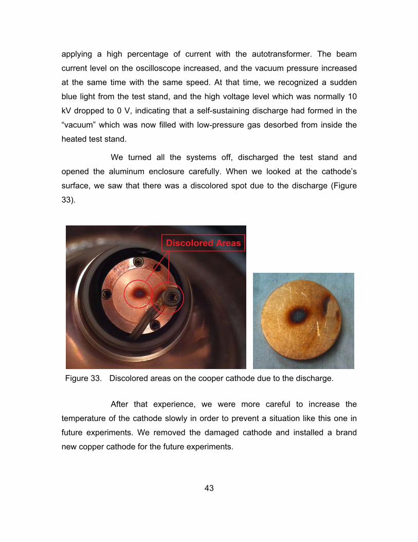
We turned all the systems off, discharged the test stand and
opened the aluminum enclosure carefully. When we looked at the cathode’s
surface, we saw that there was a discolored spot due to the discharge (Figure
33).
Figure 33. Discolored areas on the cooper cathode due to the discharge.
After that experience, we were more careful to increase the
temperature of the cathode slowly in order to prevent a situation like this one in
future experiments. We removed the damaged cathode and installed a brand
new copper cathode for the future experiments.

44
We thought that the variation on the vacuum level inside the
chamber could affect the electron production, and so it was recorded by hand
during our experiments; except at high temperatures, there was very little change
in vacuum pressure with cathode temperature during the actual experiments
presented here (Figure 32).
c. Averaged Laser Power
Laser power was the first key quantity, as it was used directly in the
QE calculations as the denominator to calculate the number of photons inside the
laser light beam. This value was important. Because of that, we spent most of
our time trying to achieve a stable laser power value on the power meter
program. It was recorded by hand, as well.
d. Charge Per Pulse
The charge per pulse was the second key quantity in the
experiment, because it gave us the number of emitted photoelectrons, and we
used it as the numerator in the QE calculation. An intelligent tool inside the
oscilloscope helped us to calculate the area. As is known, the area under a
current vs. time graph gives us the amount of charge (Equation 3.3).
Q = I t dt (3.3)
We defined the left and right boundaries of the pulse by using
vertical lines; the tool integrated the area under the curve between the two of
them and displayed the result. Then we recorded it by hand. Actually, the signal
recorded on the oscilloscope is the voltage produced by the Bergoz FCT. This is
proportional to the current passing through the FCT.

45
Figure 34. Photoelectron pulse on the screen with vertical boundaries.
e. The Peak Voltage Value of the Photoelectron Pulse on the Oscilloscope
The peak voltage value was in a supporting role at the time of this
experiment. However, during the SCL regime process, it was in the leading role.
Here, we used this value as confirmation of whether we went beyond the SCL
regime or not while we were conducting the experiment.
4. Heating the Cathode up to 400K
We did not heat the cathode suddenly to 400 K, but rather increased the
temperature in 50 K increments (Figure 35). It was important for us to detect the
QE values while the temperature was increasing up to 400 K to observe the
behavior of the cathode sample. Whenever we reached the next data-collection
temperature level, it was almost stable during the data collection process.

46
Figure 35. Image of temperature rise on computer software.
D. PROCESSING THE RAW DATA
We collected enough required data from the test stand. However, they
were not useful for calculating the QE until we processed them. At this time, we
had to convert them to the number of electrons and protons.
1. Photon Number Calculation
We knew the laser wavelength and measured the laser power, which
allowed us to determine the number of photons. Equation 4.1 gives us the
amount of one photon’s energy - E
hc
E
, (4.1)
where h is the Planck’s constant, c is the speed of light, and is the photon’s
wavelength. The number of photons delivered in a single cycle (Figure 36) is
related to the average laser power by
[ ]. .
#.[ ]
P T R
photonsRR E
, (4.2)

47
where T is the transmission coefficient of the UV window (0.922) in front of the
cathode, R is the ratio (0.4285) of the beam splitter, and RR is the laser
repetition rate of the laser (10 Hz).
2. Electron Number Calculation
We recorded the area under the curve of the photoelectron signal on the
oscilloscope in order to determine the number of electrons. The area’s unit was
Vs. So, initially we divided the value by the FCT scale factor, which was 1.25
V/A, and that gave us the amount of the charge (As) carried by the
photoelectrons. If we divide this by the charge of one electron, we get the
number of electrons in that photoelectron pulse. In the schematic diagram of the
electron number calculation (Figure 36), P is the average power, which is what
our laser power meter reads, P(t) is the instantaneous power delivered by the
laser, l(t) is the instantaneous current in our test stand, and Q is the amount of
charge delivered during one cycle.
Figure 36. Schematic diagram of electron number calculation.
[ ]
#[ _ ].
Area
electronsFCT Factor e
(4.3)

48
3. Quantum Efficiency
To find the QE, we then divide Equation 4.3 by Equation 4.2, which gives
Q#electrons
QE = =P t#photons
E
(4.4)
Because our laser power meter measures the average power P rather
than the instantaneous powerP(t) , we have effectively chosen to find the QE by
comparing the number of photons and electrons delivered in one cycle, rather
than by comparing the instantaneous rates of photons reaching the cathode and
electrons leaving the cathode (Figure 37).
Figure 37. QE per cycle.
4. Peak Current Calculation
We used peak current value for defining the SCL regime earlier in this
thesis. This value was found from the peak voltage value of the photoelectron
pulse on the oscilloscope. First, it was recorded by hand, and second it was
divided by the Bergoz FCT factor (1.25 V/A). This value was not directly used

49
inside the QE calculation because our laser power meter measured average,
rather than peak or instantaneous power.
[ _ _ ]
_[ _ ]
Peak Voltage Value
Peak CurrentFCT Factor
(4.5)
E. ANALYZING THE DATA
We conducted the experiment, gathered the values, and processed the
raw data as discussed above. For both samples, we took data at seven different
temperature conditions between 85 K and 400 K.
In this section, we present two types of graphs for each sample. Initially,
we are presenting graphs composed of the number of photons on the horizontal
scale and electrons on the vertical scale. Each graph contains several small
circles which represent the data derived from the stand during the experiment,
calculated by the equations mentioned earlier. The lower boundary (low-power
end) on the data was set by the nonlinear response at the detector (need to keep
the power greater than 5 mW on it), and the upper boundary (high-power end) on
the data was set by the need to operate below the SCL (less than 4 mW on the
cathode).
Three lines were overlaid on each of these graphs. One of them is a linear
fit to the data (red); the slope of this line corresponds to the ratio of electrons to
photons and, therefore, the QE. The other two lines (blue) are intended to show
the boundary of the data. Therefore, the difference between the slopes of these
lines and of the linear fit is a measure of the error in our measurement of QE.
These boundary lines are only shown in Figures 38 and 46 to demonstrate how
the error estimates were determined.
The second type of graph, the eighth for each cathode material, contains
the QE values and error estimates for each of the tested cathode temperatures.

50
1. Copper
What follows are seven graphs that show the QE values at different
temperature conditions for copper and one summary graph.
Figure 38. Results for copper at 85 K.

51
Figure 39. Results for copper at 150 K.
Figure 40. Results for copper at 200 K.

52
Figure 41. Results for copper at 250 K.
Figure 42. Results for copper at 300 K.

53
Figure 43. Results for copper at 350 K.
Figure 44. Results for copper at 400 K.

54
Figure 45. Dependence of QE on temperature for copper.
2. Niobium
There are also seven graphs that show the QE values at different
temperature conditions for niobium and one summary graph.

55
Figure 46. Results for niobium at 85 K.
Figure 47. Results for niobium at 150 K.

56
Figure 48. Results for niobium at 200 K.
Figure 49. Results for niobium at 250 K.
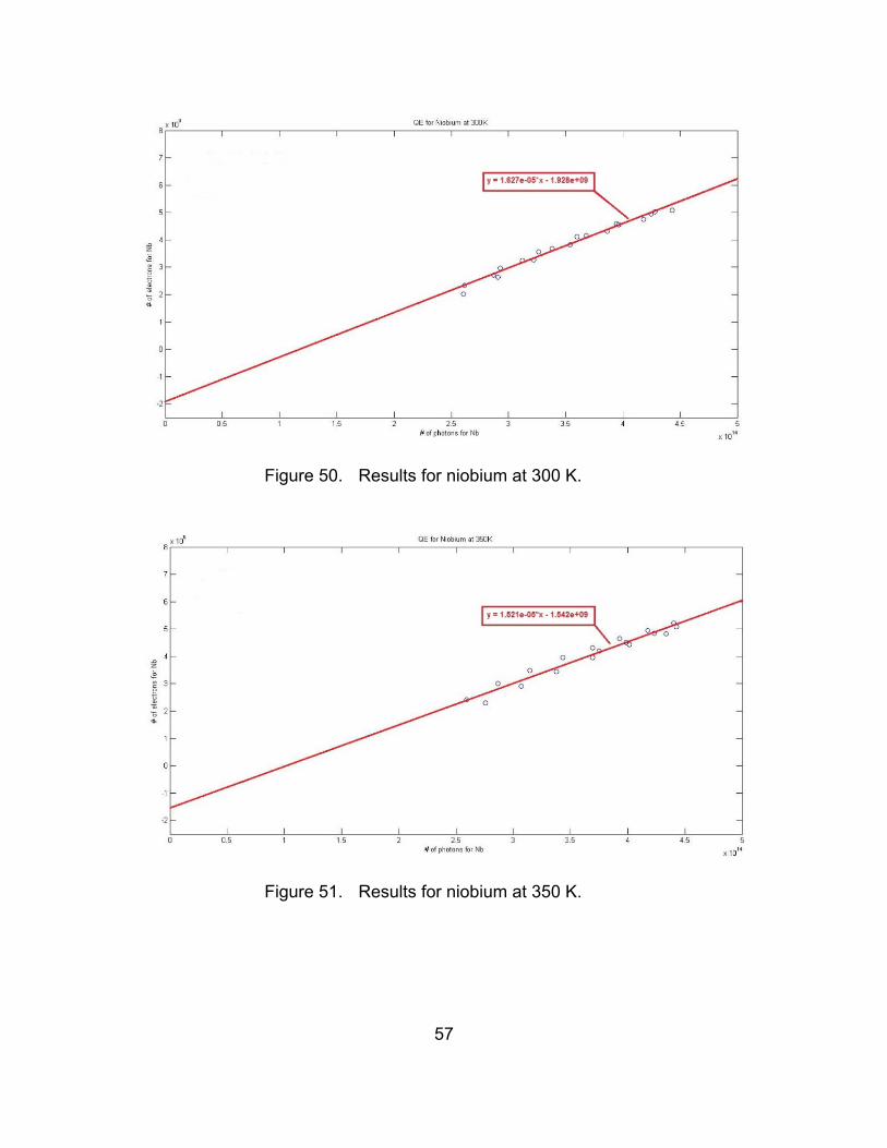
57
Figure 50. Results for niobium at 300 K.
Figure 51. Results for niobium at 350 K.

58
Figure 52. Results for niobium at 400 K.
Figure 53. Dependence of QE on temperature for niobium.

59
IV. RESULTS AND RECOMMENDATIONS FOR FUTURE WORK
A. RESULTS FOR COPPER AND NIOBIUM
The primary objective of this project was to see if there was any change in
the QE of metal photocathodes as their temperature was varied over a wide
range. To answer this simple question, we built our test stand, did experiments,
gathered data, and analyzed them as presented in previous chapters.
Figure 45 shows that for copper, there is a clear and statistically significant
increase in QE when the temperature was also increased. At 85 K, the QE was
-50.27x10 , while at 400 K, it was -51.2x10 . This represents an increase in QE by
more than a factor of four between these two temperature conditions. Over this
range, the trend was almost linear, except for the values at 200 K. The cause of
this discrepancy is unknown, but it does not obscure the clear trend evident in
the data. When we investigated the vacuum pressure level during the
experiments, it remained stable, with the exception of the points at 400 K,
indicating that vacuum pressure cannot explain the observed change in QE
(Figure 32).
We achieved higher QE values on the niobium cathode than on the
copper cathode. However, the observed dependence of QE on temperature for
niobium is much weaker than for copper, as shown in Figure 53. The highest QE
value was reached at 200 K.
This experiment found values of QE for copper and niobium that were
generally in line with those reported in the literature (Table 2). Detailed
comparisons of QE from one experiment to the next are difficult, because the QE
will depend strongly on the sample and testing conditions, which include the
cathode surface, vacuum level, and applied fields. But having a single
experimental apparatus where the temperature of the cathode can be varied
while keeping other influences (such as the cathode surface, applied fields,

60
testing procedures, and to some degree vacuum pressure) constant, as was
done here, helps us more effectively isolate the dependence of QE on
temperature.
On the other hand, the difference in the observed temperature
dependence between the copper results and the niobium results is dramatic and
unexplained. The simple theories of photoemission from metals would predict the
temperature dependence to be similar for all metals, but that is obviously not the
case. There is something going on here that needs further investigation both
experimentally and theoretically. The difference could be due to any one of the
three steps in the photoemission process: photon absorption, electron transport
to the surface and emission over the barrier. It will take a very sophisticated
experiment to determine which of these is responsible for the difference.

61
Cathode Material
QE Cathode Temperature
Vacuum Pressure around Cathode
Applied Electric Field/ Voltage
Cu 0.27 - 1.2 x 10⁻⁵ Cryogenic (85 K) to 400 K
4 - 8 x 10⁻⁷ Torr
10 kV
Cu [32] 1.4 x 10⁻⁴ Room temp. 10–8 - 10–9 Torr
10 kV
Cu [33] 1.0 x 10⁻⁴ Room temp. 10–9 Torr 3.5 MeV
Cu [34] 1.4 x 10⁻⁵ Room temp. 3.7 x 10⁻⁷ Torr
550 V
Cu [35] 5.0 x 10⁻⁴ Room temp. 10–7 Torr 130 MV/m
Nb 1.4–1.7 x 10⁻⁵ Cryogenic (85 K) to 400 K
1–5 x 10⁻⁷ Torr
10 kV
Nb [36] 2.0 x 10⁻⁶ Cryogenic (4 K) … …
Nb [37] 5.0 x 10⁻⁵ Cryogenic (2 K) … …
Nb [38] 1.0x10⁻⁷ 5.1x10⁻⁵ (*)
Room temp. 5.0 x 10⁻⁹ Torr
10 kV
Nb [39] 7.4x10⁻⁷ 6.5x10⁻⁵ (*)
Room temp. 5.0 x 10⁻⁹ Torr
10 kV
Nb [40] 1.2 x 10⁻⁵ Room temp. … 1 kV
Nb [12] 1.0 – 2.0 x 10⁻⁶ Cryogenic (4.2 K) 10–8 Torr 29 MV/m
Table 2. Quantum efficiency for copper and niobium illuminated with 266 nm light.
Note that in Table 2, bold fond indicates results obtained in this thesis. Asterisks (*) denote values achieved after surface cleaning.

62
B. RECOMMENDATIONS FOR FUTURE WORK
As previously stated, while we were doing experiments, we utilized two
pumps to try to maintain a constant vacuum environment inside the vacuum
chamber. However, this situation could not be provided at all times. Whenever
we increased the cathode temperature from a low level to a higher level, we
observed that the vacuum level started to increase, as well. Although, we waited
long enough after changing the cathode temperature to allow the system to reach
its previous vacuum level, we could not achieve the UHV vacuum condition,
especially for high temperatures, such as 300 K, 350 K, and 400 K. In the future
more powerful vacuum pumps can be used to supply a more stable vacuum
environment around the cathode during the experiment process, and the system
should be baked out at high temperatures to remove all adsorbed gases.
There is room for improvement in other areas, also. If the high voltage
could be raised from 10 kV to a much higher value, such as 100 kV, the space
charge limited regime could be avoided more easily, and higher laser powers
could be used. This requires a more advanced design of the cathode-anode
system, though, and would also require shielding and safety procedures to
protect experimenters from ionizing radiation.
The laser power detector and meter were not the best ones for this
experiment, and the power meter was working at the very low limit of its
sensitivity. The laser light was only present for 5 ns every 100 ms, but the
detector was measuring power during the whole interval. This caused uncertainty
in the measurements. A detector that could measure the energy of each pulse
during the short pulse time instead of integrating the power over all time would be
a better choice and should give better and more accurate results
Finally, a potential source of error here is the degree to which the surface
of these metals had been oxidized or contaminated. A potential way to deal with
this is to clean the surface during testing, for example using bombardment by
Argon ions.

63
LIST OF REFERENCES
[1] J. Cook, “High-energy laser weapons since the early 1960s,” Optical Eng., vol. 52, no. 2, pp. 021007–021007, 2013.
[2] E. T. Gerry and D. A. Leonard, “Measurement of 10.6‐μ CO2 laser transition probability and optical broadening cross sections,” Appl. Physics Letters, vol. 8, no. 9, pp. 227–229, 1966.
[3] J. R. Albertine, “Recent high-energy laser system tests using the MIRACL/SLBD,” in OE/LASE ‘93: Optics, Electro-Optics, & Laser Applications in Science& Engineering, pp. 229–239 Int. Soc. for Optics and Photonics, vol. 1871, 1993.
[4] “Laser,” [Online], Available: http://en.wikipedia.org/wiki/Laser [accessed 14 Dec 2012].
[5] W B. Colson and A. M. Sessler, “Free electron lasers,” Annu. Rev. of Nucl. and Particle Sci., vol. 35, no. 1, pp. 25–54, 1985.
[6] J.R. Harris, (2013, Feb. 25). E-mail message to author.
[7] J. R. Cook and J. R. Albertine, “The navy’s high energy laser weapon system,” in Proc.-Spie The Int. Soc. for Optical Eng., pp. 264–271,1997.
[8] “ONR Free Electron Laser,” [Online], Available: www.onr.navy.mil/en/Media-Center/Fact-Sheets/Free-Electron-Laser.aspx [accessed 14 Dec 2012].
[9] W. B. Colson, “Introduction to the free electron laser,” PH 4858, class notes, Naval Postgraduate School, Monterey, CA, 2012.
[10] “RI Research Instrument GmbH,” [Online], Available: www.research-instruments.de/frontend/products-european-xfel [accessed 14 Jun 2013].
[11] S. P. Niles, W. B. Colson, K. L. Ferguson, J. R. Harris, J. W. Lewellen, B. Rusnak, R. Swent, “NPS prototype superconducting 500 MHz quarter-wave gun update,” in Proc. of the 20l0 FEL Conf., Malmö, Sweden, 2010, pp. 457–460.
[12] J. R. Harris, K. L. Ferguson, J. W. Lewellen, S. P. Niles, B. Rusnak, R. L. Swent, W. B. Colson, T. I. Smith, C. H. Boulware, T. L. Grimm, P. R. Cunningham, M. S. Curtin, D. C. Miccolis, D. J. Sox, W. S. Graves, “Design and operation of a superconducting quarter-wave electron gun,” Phys. Rev. Special Topics-Accelerators and Beams, vol. 14, no. 5, p. 053501, 2011.

64
[13] A.I. Yilmaz, “Development and experimental operation of a flashboard plasma cathode test stand,” M.S. thesis, Applied Physics Dept., Naval Postgraduate School, Monterey, CA,, 2012.
[14] J.Z. Buchwald, The Creation of Scientific Effects: Heinrich Hertz and Electric Waves. Chicago, IL: Univ. of Chicago Press, 1994.
[15] A. Einstein, Sidelights on relativity, Dover, Mineola, New York, 1983.
[16] A.H. Sommer, Photoemissive Materials. New York: John Wiley & Sons, 1968, pp. 21–26.
[17] X.J. Wang, M. Babzien, R. Malone, Z. Wu, “Mg cathode and its thermal emittance,” Proc. of LINAC 2002, Gyeongju, Korea, pp. 142–144, 2002.
[18] D. H. Dowell., I. Bazarov, B. Dunham, K. Harkay, C. Hernandez-Garcia, R. Legg, H. Padmore, T. Rao, J. Smedley, and W. Wan, “Cathode R&D for future light sources,” Nuclear Instruments and Methods in Physics Research Section A: Accelerators, Spectrometers, Detectors and Associated Equipment, vol. 622, no. 3, pp. 685–697, 2010.
[19] K. L. Jensen and E. J. Montgomery, “Photoemission theory and the development of high performance photocathodes,” J. of Computational and Theoretical Nanosci., vol. 6, no. 8, pp. 1754–1769, 2009.
[20] K. L. Jensen, “Electron emission physics,” Advances in Imaging and Electron Physics, vol.149, pp. 147–279, 2007.
[21] E. J. Montgomery, D. W. Feldman, P. G. O’Shea, J. C. Jimenez, J. R. Harris, K. L. Jensen, “Cesium emission in dispenser photocathodes,” Proc. of the 20l0 FEL Conf., pp. 422–424, 2010.
[22] J. C. Jimenez, . “A systematic cathode study - Activation of a thermionic cathode, and measuring cesium evaporation from a dispenser photocathode.” M.S. thesis, Applied Physics Dept., Naval Postgraduate School, Monterey, CA, 2010.
[23] T. Maruyama, R. Prepost, E. L. Garwin, C. K. Sinclair, B. Dunham and S. Kalem, “Enhanced electron spin polarization in photoemission from thin GaAs,” Appl. Physics Lett., vol. 55, no. 16, pp. 1686–1688, 1989.
[24] C. K. Sinclair, “Recent advances in polarized electron sources,” Proc. of the IEEE Particle Accelerator Conf., vol. 1, pp. 65–69, 1999.
[25] R. J. Umstattd., C. A. Schlise, and F. Wang. “Gas evolution during operation of a CsI-coated carbon fiber cathode in a closed vacuum system,” Plasma Science, IEEE Trans., vol. 33, no. 2, pp.901–910, 2005.

65
[26] K. L. Jensen, N. A. Moody, D. W. Feldman, E. J. Montgomery, and P. G. O’Shea. “Photoemission from metals and cesiated surfaces.” J. of Appl. Physics, vol. 102, no. 7, p. 074902–074902, 2007.
[27] K. L. Jensen, P. G. O’Shea, D. W. Feldman, and N. A. Moody. “Theoretical model of the intrinsic emittance of a photocathode,” Appl. Physics Lett., vol. 89, no. 22,pp. 224103–224103, 2006.
[28] N. A. Moody, Kevin L. Jensen, Donald W. Feldman, Eric J. Montgomery, and Patrick G. OShea. “Factors affecting performance of dispenser photocathodes,” J. of Appl. Physics, vol.102, no. 10, pp. 104901–104901, 2007.
[29] J. G. Neumann, J. R. Harris, B. Quinn and P. G. O’Shea, “Production of photoemission-modulated beams in a thermionic electron gun,” Rev.of Sci. Instrum., vol. 76, no. 3, pp. 033303–033303, 2005.
[30] A. B. Baxter, “Cathode stalk cooling system for the MK1 quarterwave gun.” M.S. thesis, Applied Physics Dept., Naval Postgraduate School, Monterey, CA, 2012.
[31] J.R. Harris. (2013, May 20). E-mail message to author.
[32] T. Srinivasan-Rao, J. Fischer, and T. Tsang, “Photoemission studies on metals using picosecond ultraviolet laser pulses,” J. of Appl. Physics, vol. 69, no. 5, pp. 3291–3296,1991.
[33] P. Davis, G. Hairapetian, C. Clayton, C. Joshi, S. Hartman, S. Park, C. Pellegrini, and J. Rosenzweig, “Quantum efficiency measurements of a copper photocathode in an RF electron gun,” Proc. of the IEEE Particle Accelerator Conference, pp. 2976–2978,1993.
[34] E. B. Sozer, Chunqi Jiang, Martin A. Gundersen, and R. J. Umstattd, “Quantum efficiency measurements of photocathode candidates for back-lighted thyratrons.” Dielectrics and Electrical Insulation, IEEE Trans. vol. 16, no. 4, pp. 993–998, 2009.
[35] X. J. Wang, M. Babzien, K. Batchelor, I. Ben-Zvi, R. Malone, I. Pogorelsky, X. Qui, J. Sheehan, J. Sharitka, and T. Srinivasan-Rao, “Experimental characterization of the high-brightness electron photoinjector,” Nuclear Instruments and Methods in Physics Research Section A: Accelerators, Spectrometers, Detectors and Associated Equipment, vol. 375, no. 1, pp. 82–86, 1996.

66
[36] T. Srinivasan-Rao, I. Ben-Zvi, A. Burrill, H. Hahn, D. Kayran, Y. Zhao, and M. Cole. “Photoemission studies on BNL/AES/JLAB all niobium, superconducting RF injector.” In Proc. IEEE of the Particle Accelerator Conference, pp. 2556–2558, 2005.
[37] T. Srinivasan-Rao, I. Ben-Zvi, A. Burrill, G. Citver, A. Hershcovitch, D. Pate, A. Reuter et al., “Design, construction and status of all niobium superconducting photoinjector at BNL,” Proc. IEEE of the Particle Accel. Conf, vol. 1, pp. 92–94, 2003.
[38] Q. Zhao, Triveni Srinivasan-Rao, and Mike Cole. “Tests of niobium cathode for the superconducting radio frequency gun,” Proc. IEEE of the Particle Accelerator Conference, vol. 3, pp. 2047–2049, 2003.
[39] J. Smedley, T. Rao, and Q. Zhao. “Photoemission studies on niobium for superconducting photo injectors,” J. of Appl. Physics, vol. 98, no. 4,pp. 043111–043111, 2005.
[40] J. Smedley, Triveni Rao, B. N. L. John Warren, and D. E. S. Y. Jacek Sekutowicz, “Photoemission Properties of Lead.” Proc. European Part. Accel. Conf., p. 1126, 2004.
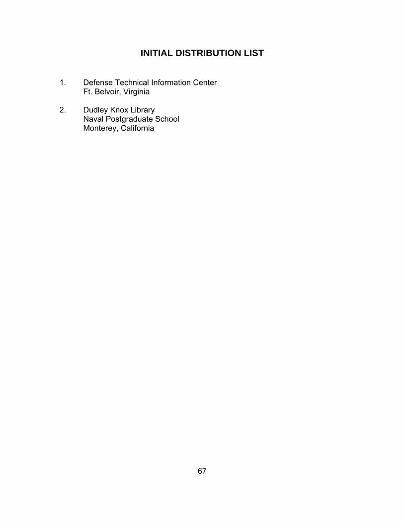
67
INITIAL DISTRIBUTION LIST
1. Defense Technical Information Center Ft. Belvoir, Virginia 2. Dudley Knox Library Naval Postgraduate School Monterey, California