NAVAL POSTGRADUATE · PDF fileiii Approved for public release; distribution is unlimited A PRELIMINARY INVESTIGATION INTO CNO AVAILABILITY SCHEDULE OVERRUNS Joseph L. Caprio

NAVAL

POSTGRADUATE

SCHOOL

MONTEREY, CALIFORNIA

THESIS

Approved for public release; distribution is unlimited

A PRELIMINARY INVESTIGATION INTO CNO AVAILABILITY SCHEDULE OVERRUNS

by

Joseph L. Caprio Daniel Leszczynski

June 2012

Thesis Advisors: Clifford Whitcomb Patricia Jacobs

THIS PAGE INTENTIONALLY LEFT BLANK

i

REPORT DOCUMENTATION PAGE Form Approved OMB No. 0704–0188 Public reporting burden for this collection of information is estimated to average 1 hour per response, including the time for reviewing instruction, searching existing data sources, gathering and maintaining the data needed, and completing and reviewing the collection of information. Send comments regarding this burden estimate or any other aspect of this collection of information, including suggestions for reducing this burden, to Washington headquarters Services, Directorate for Information Operations and Reports, 1215 Jefferson Davis Highway, Suite 1204, Arlington, VA 22202–4302, and to the Office of Management and Budget, Paperwork Reduction Project (0704–0188) Washington DC 20503. 1. AGENCY USE ONLY (Leave blank)

2. REPORT DATE June 2012

3. REPORT TYPE AND DATES COVERED Master’s Thesis

4. TITLE AND SUBTITLE A Preliminary Investigation into CNO Availability Schedule Overruns 6. AUTHOR(S) Joseph L. Caprio, Daniel Leszczynski

5. FUNDING NUMBERS

7. PERFORMING ORGANIZATION NAME(S) AND ADDRESS(ES) Naval Postgraduate School Monterey, CA 93943–5000

8. PERFORMING ORGANIZATION REPORT NUMBER

9. SPONSORING /MONITORING AGENCY NAME(S) AND ADDRESS(ES) N/A

10. SPONSORING/MONITORING AGENCY REPORT NUMBER

11. SUPPLEMENTARY NOTES The views expressed in this thesis are those of the author and do not reflect the official policy or position of the Department of Defense or the U.S. Government. IRB Protocol number ______N/A______.

12a. DISTRIBUTION / AVAILABILITY STATEMENT Approved for public release; distribution is unlimited

12b. DISTRIBUTION CODE A

13. ABSTRACT (maximum 200 words) A naval vessel’s “availability” is a scheduled period of time, normally conducted in a shipyard, to perform maintenance on and modernization of the vessel and its systems. The four public naval shipyards are continually challenged to complete depot-level, CNO availabilities on schedule. A naval vessel’s late return to the fleet results in the decrease in operational readiness due to the reduced number of operational days available for these vessels. Subject-matter experts hypothesize that factors such as inadequate planning for resources, quantity of overtime, and quantity of work stoppages experienced contribute to availability lateness. Data collected by the shipyards are analyzed to investigate factors influencing late completion of availabilities. The analysis suggests that carrier availabilities tend to finish on schedule more often than submarine availabilities; timely availabilities tend to have a higher cost performance ratio than late availabilities; late availabilities tend to charge less for work per month in man-days than the budgeted amount of planned work; and availabilities that finish on schedule tend to have fewer work stoppages prior to start of the availability than the later completing ones.

15. NUMBER OF PAGES

141

14. SUBJECT TERMS CNO Availability, Naval Shipyards, Schedule Overrun, Availability Lateness, Cost Performance, Budgeted Quantity Work Performed, Actual Quantity Work Performed, Availability Delay, Work Stoppages 16. PRICE CODE

17. SECURITY CLASSIFICATION OF REPORT

Unclassified

18. SECURITY CLASSIFICATION OF THIS PAGE

Unclassified

19. SECURITY CLASSIFICATION OF ABSTRACT

Unclassified

20. LIMITATION OF ABSTRACT

UU NSN 7540–01–280–5500 Standard Form 298 (Rev. 2–89) Prescribed by ANSI Std. 239–18

ii


iii

Approved for public release; distribution is unlimited

A PRELIMINARY INVESTIGATION INTO CNO AVAILABILITY SCHEDULE OVERRUNS

Joseph L. Caprio Lieutenant, United States Navy

B.S., University of Arizona, 2007

Daniel Leszczynski Lieutenant Junior Grade, United States Navy B.S., Rensselaer Polytechnic Institute, 2003

Submitted in partial fulfillment of the requirements for the degree of

MASTER OF SCIENCE IN SYSTEMS ENGINEERING

from the

NAVAL POSTGRADUATE SCHOOL JUNE 2012

Author: Joseph L. Caprio Daniel Leszczynski

Approved by: Clifford Whitcomb Thesis Advisor

Patricia Jacobs Thesis Advisor

Clifford Whitcomb Chair, Department of Systems Engineering

iv


v

ABSTRACT

A naval vessel’s “availability” is a scheduled period of time, normally conducted in a

shipyard, to perform maintenance on and modernization of the vessel and its systems.

The four public naval shipyards are continually challenged to complete depot-level, CNO

availabilities on schedule. A naval vessel’s late return to the fleet results in the decrease

in operational readiness due to the reduced number of operational days available for these

vessels. Subject-matter experts hypothesize that factors such as inadequate planning for

resources, quantity of overtime, and quantity of work stoppages experienced contribute to

availability lateness. Data collected by the shipyards are analyzed to investigate factors

influencing late completion of availabilities. The analysis suggests that carrier

availabilities tend to finish on schedule more often than submarine availabilities; timely

availabilities tend to have a higher cost performance ratio than late availabilities; late

availabilities tend to charge less for work per month in man-days than the budgeted

amount of planned work; and availabilities that finish on schedule tend to have fewer

work stoppages prior to start of the availability than the later completing ones.

vi


vii

TABLE OF CONTENTS

I. INTRODUCTION........................................................................................................1 A. PURPOSE.........................................................................................................1 B. PROBLEM STATEMENT .............................................................................1 C. SUBJECT-MATTER EXPERT INTERVIEWS ..........................................2 D. RESEARCH QUESTIONS.............................................................................4 E. BENEFIT OF STUDY.....................................................................................4 F. SCOPE OF THE THESIS...............................................................................5

II. CNO AVAILABILITY................................................................................................7 A. INTRODUCTION............................................................................................7 B. CNO AVAILABILITIY DEFINED ...............................................................7

1. Navy Maintenance Program ...............................................................7 2. CNO Availability Stakeholders ..........................................................9

C. CNO AVAILABILITY PLANNING PROCESS ..........................................9 D. AVAILABILITY TYPES AND MAINTENANCE PHILOSOPHIES .....10 E. SUMMARY ....................................................................................................12

III. TOP-LEVEL SHIPYARD PERFORMANCE DATA ANALYSIS ......................13 A. INTRODUCTION..........................................................................................13 B. DATA SET DESCRIPTION.........................................................................13 C. COMPARING THE SHIPYARDS ..............................................................14 D. COMPARING THE COST PERFORMANCE MEANS...........................20 E. DAYS LATE VERSUS AVAILABILITY LENGTH .................................24 F. NUMBER OF AVAILABILITIES IN THE SHIPYARD VERSUS

THE NUMBER OF DAYS LATE AS A PERCENTAGE OF PLANNED AVAILABILITY LENGTH .....................................................29

G. EFFECTS OF WINTER MONTHS ON AVAILABILITY LATENESS.....................................................................................................37

H. IMPACT OF CARRIER AVAILABILITIES ON SUBMARINE AVAILABILITIES ........................................................................................39

I. IMPACT OF PERSONNEL RESOURCES ON AVAILABILITY LATENESS.....................................................................................................42

J. SUMMARY ....................................................................................................46

IV. AVAILABILITY EXECUTION...............................................................................47 A. INTRODUCTION..........................................................................................47 B. NETWORK SCHEDULING ........................................................................47

1. Network Fundamentals .....................................................................47 a. Float.........................................................................................49

2. Scheduling Problems .........................................................................50 C. THEORY OF CONSTRAINTS....................................................................50

1. Critical Chain Management..............................................................52 D. WORK STOPPAGE......................................................................................53 E. WEB AIM-NG SOFTWARE........................................................................54

viii

1. Execution Priorities ...........................................................................54 F. SUMMARY ....................................................................................................56

V. WORK STOPPAGE ANALYSIS.............................................................................57 A. INTRODUCTION..........................................................................................57 B. RAW WORK STOPPAGE DATA...............................................................57

1. Description of the Data......................................................................60 2. Data Organization..............................................................................62

C. WORK STOPPAGES BY LENGTH...........................................................64 1. Complete Work Stoppage Data ........................................................64 2. Red Color-Coded Work Stoppage Data ..........................................66

D. WORK STOPPAGES BY QUANTITY.......................................................68 E. WORK STOPPAGES BY TIME-IN-AVAILABILITY.............................69

1. Pre-availability Work Stoppage Ratio .............................................71 F. SUMMARY ....................................................................................................73

VI. CONCLUSION AND FUTURE STUDIES .............................................................75 A. SUMMARY OF STUDIES............................................................................75 B. ADDRESSING THE CONCERNS OF THE SUBJECT MATTER

EXPERTS .......................................................................................................76 C. CONCLUSIONS AND RECOMMENDATIONS.......................................77

APPENDIX A: TOP LEVEL SHIPYARD DATA..............................................................83 A. SHIPYARD AVAILABILITY COMPLETION DATA.............................83 B. SHIPYARD GANTT CHARTS....................................................................85

APPENDIX B: AQWP AND BQWP STATISTICAL COMPARISON RESULTS........89 A. AQWP AND BQWP PER MONTH FOR LATE AVAILABILITIES.....89 B. AQWP AND BQWP PER MONTH FOR TIMELY

AVAILABILITIES ........................................................................................91 C. STANDARD ERRORS FOR MEAN AQWP AND BQWP PER

MONTH..........................................................................................................93

APPENDIX C: WORK STOPPAGE DATA BY LENGTH..............................................95 A. COMPLETE WORK STOPPAGE DATA SETS.......................................95 B. RED COLOR-CODED WORK STOPPAGE DATA SETS......................99

APPENDIX D: WORK STOPPAGE DATA BY QUANTITY........................................103 A. COMPLETE WORK STOPPAGE DATA SETS.....................................103 B. RED COLOR-CODED WORK STOPPAGE DATA SETS....................103

APPENDIX E: WORK STOPPAGES BY TIME-IN-AVAILABILITY........................105 A. COMPLETE WORK STOPPAGE DATA SETS.....................................105 B. RED COLOR-CODED WORK STOPPAGE DATA SETS....................111

LIST OF REFERENCES....................................................................................................117

INITIAL DISTRIBUTION LIST .......................................................................................119

ix

LIST OF FIGURES

Figure 1. Historical On Time Percentages (From NAVSEA 04X 2011)..........................2 Figure 2. Sample SEA 04X Historical Availability Data................................................14 Figure 3. Number of Completed Availabilities at Norfolk Naval Shipyard ...................15 Figure 4. Number of Completed Availabilities at Pearl Harbor Naval Shipyard............16 Figure 5. Number of Completed Availabilities at Portsmouth Naval Shipyard..............17 Figure 6. Number of Completed Availabilities at Puget Sound Naval Shipyard............18 Figure 7. Frequency of Cost Performance Ratios for Late and Timely Availabilities....24 Figure 8. Days Late Percentage as a Function of Planned Availability Length..............27 Figure 9. Number of Days Late as a Function of Planned Availability Length..............28 Figure 10. Availabilities in Norfolk Naval Shipyard between 2005 and 2009 .................30 Figure 11. Days Late Percentage as a Function of the Number of Availabilities

Underway in the Shipyard ...............................................................................33 Figure 12. Days Late Percentage Trends from 2005 to 2009............................................34 Figure 13. Days Late Percentage Trends from 2003 to 2011............................................36 Figure 14. Days Late Percentage as a Function of Percentage of Availability Duration

in Inclement Weather Months at Puget Sound Naval Shipyard ......................38 Figure 15. Days Late Percentage as a Function of Percentage of Availability Duration

in Inclement Weather Months at Portsmouth Naval Shipyard ........................38 Figure 16. Days Late Percentage as a Function of Carrier Impact Factor ........................41 Figure 17. Carrier Impact Factor as a Function of Planned Availability Length..............42 Figure 18. Network Diagram Example (After Langford 2011) ........................................48 Figure 19. Critical Chain Colored in Red (After Langford 2011).....................................53 Figure 20. EPR Process Diagram (After NAVSEA 04X 2009)........................................55 Figure 21. Actual Availability Lengths Compared with Data Collection Timeframe ......61 Figure 22. Quantity of MAT, IC, and TD Work Stoppages by Time-in-Availability ......70 Figure 23. Pre-Availability Work Stoppage Ratio at 50% Point of Planned

Availability ......................................................................................................72 Figure 24. Availabilities at Norfolk Naval Shipyard from 2005 to 2009..........................85 Figure 25. Availabilities at Pearl Harbor Naval Shipyard from 2005 to 2009..................86 Figure 26. Availabilities at Portsmouth Naval Shipyard from 2005 to 2009....................87 Figure 27. Availabilities at Puget Sound Naval Shipyard from 2005 to 2009..................88 Figure 28. EISENHOWER (CVN 69) PIA.....................................................................105 Figure 29. GEORGE WASHINGTON (CVN 73) SRA .................................................106 Figure 30. COLUMBUS (SSN 762) DSRA....................................................................107 Figure 31. MICHIGAN (SSGN 727) MMP....................................................................108 Figure 32. JOHN C STENNIS (CVN 74) PIA................................................................109 Figure 33. NORFOLK (SSN 714) CM ...........................................................................110 Figure 34. EISENHOWER (CVN 69) PIA.....................................................................111 Figure 35. GEORGE WASHINGTON (CVN 73) SRA .................................................112 Figure 36. COLUMBUS (SSN 762) DSRA....................................................................113 Figure 37. MICHIGAN (SSGN 727) MMP....................................................................114 Figure 38. JOHN C STENNIS (CVN 74) PIA................................................................115 Figure 39. NORFOLK (SSN 714) CM ...........................................................................116

x


xi

LIST OF TABLES

Table 1. Availability Completions For Norfolk Naval Shipyard...................................15 Table 2. Availability Completions For Pearl Harbor Naval Shipyard...........................16 Table 3. Availability Completions For Portsmouth Naval Shipyard .............................17 Table 4. Availability Completions For Puget Sound Naval Shipyard ...........................18 Table 5. Percentage of Completed Availabilities Ended Late from 2001 to 2011 ........19 Table 6. Percentage of Submarine Availabilities Ended Late per Shipyard..................19 Table 7. Percentage of Carrier Availabilities Ended Late per Shipyard........................20 Table 8. Mean Cost Performances and Overtime Percentages for the Four

Shipyards..........................................................................................................21 Table 9. Results in Testing for Significant Difference of the Means for Cost

Performance and Overtime Percentage............................................................22 Table 10. Cost Performance Data Comparison for Late and Timely Availabilities ........23 Table 11. Lateness Statistics of Availabilities of Various Lengths .................................25 Table 12. Lateness Statistics of Submarine and Carrier Availabilities of Various

Lengths.............................................................................................................26 Table 13. Lateness Frequencies of Availabilities of Various Lengths ............................28 Table 14. Days Late Percentage Statistics with Various Amounts of Availabilities

Underway in the Shipyard ...............................................................................32 Table 15. Lateness Statistics over Time...........................................................................35 Table 16. Carrier Impact Factors and Submarine Availability Lateness Statistics at

Puget Sound Naval Shipyard ...........................................................................40 Table 17. AQWP per Month and BQWP per Month Statistics for Late and Timely

Availabilities ....................................................................................................43 Table 18. AQWP per Month and BQWP per Month Statistics for Various

Availability Types............................................................................................44 Table 19. AQWP per Month and BQWP per Month Statistics for Various

Availability Types............................................................................................45 Table 20. AQWP and BQWP divided by Planned Availability Length in Months.........46 Table 21. Work Stoppage Reasons Organized Based on Constraint Type......................52 Table 22. Sample SEA 04X Work Stoppage Data...........................................................58 Table 23. High Level Work Stoppage Data Characteristics ............................................60 Table 24. Work Stoppage Analysis Availability Summary.............................................62 Table 25. Sample Macro Output ......................................................................................63 Table 26. Work Stoppage Reason Mean Length Summary.............................................65 Table 27. Relative Work Stoppage Duration Rankings...................................................66 Table 28. Red Color-Coded Work Stoppage Reason Mean Length Summary ...............67 Table 29. Relative Red-Color Coded Work Stoppage Duration Rankings......................68 Table 30. Percentage of Availability’s Total Red Color-Coded Work Stoppages ..........68 Table 31. Complete Data Set Pre-Availability Work Stoppage Ratio.............................71 Table 32. Norfolk Naval Shipyard Availability Completion Based on Days Late..........83 Table 33. Pearl Harbor Naval Shipyard Availability Completion Based on Days Late..83 Table 34. Portsmouth Naval Shipyard Availability Completion Based on Days Late ....84

xii

Table 35. Puget Sound Naval Shipyard Availability Completion Based on Days Late ..84 Table 36. T-test Results Comparing Means of AQWP/Month (Actual Duration) and

BQWP/Month (Planned Duration) for Late Availabilities ..............................89 Table 37. T-test Results Comparing Means of AQWP/Month (Planned Duration)

and BQWP/Month (Planned Duration) for Late Availabilities .......................90 Table 38. T-test Results Comparing Means of AQWP/Month (Actual Duration) and

BQWP/Month (Planned Duration) for Timely Availabilities..........................91 Table 39. T-test Results Comparing Means of AQWP/Month (Planned Duration)

and BQWP/Month (Planned Duration) for Timely Availabilities...................92 Table 40. Standard Errors for Mean AQWP per Month and Mean BQWP per Month

in Man-Days.....................................................................................................93 Table 41. EISENHOWER (CVN 69) PIA.......................................................................95 Table 42. GEORGE WASHINGTON (CVN 73) SRA ...................................................96 Table 43. COLUMBUS (SSN 762) DSRA......................................................................96 Table 44. MICHIGAN (SSGN 727) MMP......................................................................97 Table 45. JOHN C STENNIS (CVN 74) PIA..................................................................97 Table 46. NORFOLK (SSN 714) CM .............................................................................98 Table 47. EISENHOWER (CVN 69) PIA.......................................................................99 Table 48. GEORGE WASHINGTON (CVN 73) SRA ...................................................99 Table 49. COLUMBUS (SSN 762) DSRA....................................................................100 Table 50. MICHIGAN (SSGN 727) MMP....................................................................100 Table 51. JOHN C STENNIS (CVN 74) PIA................................................................101 Table 52. NORFOLK (SSN 714) CM ...........................................................................101 Table 53. Quantity of Work Stoppages..........................................................................103 Table 54. Quantity of Red Color-Coded Work Stoppages ............................................103 Table 55. EISENHOWER (CVN 69) PIA.....................................................................105 Table 56. GEORGE WASHINGTON (CVN 73) SRA .................................................106 Table 57. COLUMBUS (SSN 762) DSRA....................................................................107 Table 58. MICHIGAN (SSGN 727) MMP....................................................................108 Table 59. JOHN C STENNIS (CVN 74) PIA................................................................109 Table 60. NORFOLK (SSN 714) CM ...........................................................................110 Table 61. Pre-availability Work Stoppage Ratio ...........................................................110 Table 62. EISENHOWER (CVN 69) PIA.....................................................................111 Table 63. GEORGE WASHINGTON (CVN 73) SRA .................................................112 Table 64. COLUMBUS (SSN 762) DSRA....................................................................113 Table 65. MICHIGAN (SSGN 727) MMP....................................................................114 Table 66. JOHN C STENNIS (CVN 74) PIA................................................................115 Table 67. NORFOLK (SSN 714) CM ...........................................................................116 Table 68. Pre-availability Work Stoppage Ratio ...........................................................116

xiii

LIST OF ACRONYMS AND ABBREVIATIONS

%OT Percent of overtime man-days of total project man-days executed

AQWP Actual Quantity of Work Performed

AS Emory S. Land class Submarine Tender

AWP Availability Work Package

BQWP Budgeted Quantity of Work Performed

CM Continuous Maintenance

CNO Chief of Naval Operations

CP Cost Performance measured as BQWP/AQWP

CVN Nuclear Powered Aircraft Carrier

DMP Depot Modernization Period

DPIA Docking Planned Incremental Availability

DPL Daily Priority List

DPMA Docking Phased Maintenance Availability

DSRA Docking Selected Restricted Availability

EOC Engineered Operating Cycle

EOH Engineered Overhaul

EPR Execution Priorities

ERO Engineered Refueling Overhaul

ESDRA Extended Docking Selected Restricted Availability

IA Inactivation Availability

IC Interference/Coordination Work Stoppage

IMF Intermediate Maintenance Facility

IDD Interim Dry-Docking

JS Job Summaries

LHD Landing Helicopter Dock Ship

LMA Lead Maintenance Activity

MAT Material Work Stoppage

MMP Major Maintenance Period

MTS Moored Training Ship

NAVSEA Naval Sea Systems Command

xiv

NNSY Norfolk Naval Shipyard

NSA Naval Supervisory Authority

OT Overtime in man-days

PHNSY Pearl Harbor Naval Shipyard and IMF

PIA Planned Incremental Availability

PIRA Pre-Inactivated Restricted Availability

PNSY Portsmouth Naval Shipyard

PROG Progressive Maintenance

PSNSY Puget Sound Naval Shipyard and IMF

QAC Quantity at Completion

RSC Resource Work Stoppage

SAF Safety Work Stoppage

SEA 04 Deputy Cmdr for Logistics, Maintenance and Industrial Operations

SEA 04X Assistant Deputy Commander Industrial Operations

SEA07 Deputy Commander for Undersea Warfare

SRA Selected Restricted Availability

SSBN Ballistic Missile Submarine

SSGN Guided Missile Submarine

SSN Fast Attack Submarine

TD Technical Direction Work Stoppage

TL Tooling Work Stoppage

TOC Theory of Constraints

TPAV Availability Type

TWD Technical Work Document

W Workmanship/Rework

WC Work Control

xv

EXECUTIVE SUMMARY

This research explores various factors affecting the late completion of CNO availabilities.

Availabilities are defined as the time when U.S. naval vessels are made available to

maintenance activities for the accomplishment of maintenance and alterations. Timely

completion of these maintenance and alteration projects is vital to maximizing fleet

operational readiness and preventing cost overruns. Subject-matter experts hypothesize

some factors that may contribute to availability lateness, such as:

• Inadequate planning for and availability of resources

• Underestimation of new work added to the initial work package

• Excessive quantity of over-time

• Excessive amounts of work stoppages preventing adherence to the planned schedule

Data collected by the shipyards are analyzed to identify factors contributing to

late completion of availabilities.

The scope of this study covers availabilities pertaining to maintenance and

alteration projects conducted on following naval vessel hulls: CVN 68, SSN 688,

SSBN/SSGN 726, SSN 21, SSN 774, and LHD 1 class ships.

The lessons gained from this study offer areas for further research and

investigation. The results are as follows:

• Carrier availabilities finish on schedule more often than submarine availabilities (Chapter III, Section C)

• Timely availabilities tend to have a higher cost performance ratio than late availabilities (Chapter III, Section D)

• Short submarine availabilities of fewer than 200 days are more likely to possess a greater number of days late as a percentage of planned length than longer availabilities (Chapter III, Section F)

• No clear association exists between availability lateness and the number of simultaneous availabilities underway in a shipyard (Chapter III, Section G)

xvi

• The number of days late as a percentage of planned length of an availability appears to be decreasing at most shipyards after 2006 (Chapter III, Section G)

• No clear association exists between submarine availability lateness and the number of concurrent carrier availabilities (Chapter III, Section I)

• Late availabilities tend to charge less for work per month in man-days than the budgeted amount of planned work, whereas timely availabilities tend to charge more for work per month in man-days than the budgeted amount of planned work (Chapter III, Section J)

• No clear association exists between the quantity (Chapter V, Section D) or duration (Chapter V, Section C) of work stoppages during an availability and availability lateness

• Availabilities that finish on schedule tend to have fewer work stoppages prior to availability start than late availabilities (Chapter V, Section E)

The thesis begins with a top-level data analysis to gain perspective on shipyard

performance of the four Navy-owned shipyards located in Norfolk, Pearl Harbor,

Portmouth, and Puget Sound. Lateness statistics of carrier and submarine availabilities

are compared; the cost performance metric for late and timely availabilities are also

compared. To explore possible associations with availability lateness, lateness statistics

are computed for: availabilities of different scheduled lengths, availabilities conducted

with differing numbers of simultaneous availabilities underway in the shipyard,

availabilities completed in contiguous three year time periods during the years 2003 to

2011, and also for availabilities with various durations in inclement weather months.

Additionally, the possibility of an association between submarine availability lateness

and the number of simultaneous carrier availabilities underway at Puget Sound Naval

Shipyard is investigated. Finally, an analysis of the historical, top-level data compares the

estimate of charged time spent in completing project work (actual quantity of work

performed) per month with the estimated scheduled time spent to complete project work

(budgeted quantity of work performed) per month for both late and timely availabilities.

Analysis of work stoppage data investigates the effect unplanned delays, known

as work stoppages, have on availability lateness. The availability’s management team

submits work stoppages, categorized by eight different reasons, if the planned work for a

job is unable to continue. The work stoppage data are summarized in three ways in order

xvii

to display commonalities and identify trends in work stoppages that are associated with

availability lateness. The first two summaries organize the work stoppage data based on

the mean length per work stoppage and the number of work stoppages submitted per

work stoppage reason. The last summary organizes work stoppages based on the time-in-

availability of work stoppage submissions.

Expansion of this research and further in-depth studies are necessary to truly

understand the availability dynamic in regard to shipyard performance. This research,

along with its recommendations for future and continuing studies, can assist NAVSEA

and the naval shipyards leadership in understanding factors contributing to on-time and

late availabilities. In addition, this research identifies factors associated with schedule

lateness.

xviii


xix

ACKNOWLEDGMENTS

First and foremost, we thank Professor Patricia Jacobs for her patience and effort

in assisting us in our analyses and writing. With utmost appreciation, we thank Professor

Clifford Whitcomb for his tremendous guidance and support in accomplishing the feat of

this thesis. Our gratitude is extended to Professors Donald Gaver and Gary Langford for

their recommendations and vast knowledge in statistics and project management,

respectively. We also thank our Systems Engineering Program Officer, Commander

Joseph Keller, for expanding our knowledge of the Naval maintenance community and

Mrs. Mary Vizzini for all her assistance in the writing of this thesis.

Finally, this study would not have been conducted if it were not for the industry

personnel who spared their valuable time to share their insights and experiences on

shipyard work and evaluation methods. Names of those personnel include, but are not

limited to, Mike Boisseau, Lance Smith, David Kohl, and Philip Bornmeier of NAVSEA

04X, Stefanie Link of NAVSEA 07, Norm LaFleur and Eric Gendron of SUBMEPP,

Commander John Szatkowski, John Pickel, Claxton Boone, and Glen Tainter of Norfolk

Naval Shipyard, and Tom Gallagher and Jon Bogan of SURFMEPP.

Joseph Caprio:

Most importantly, I thank my wife, Megan, for her continued love, support, and

patience throughout my time here at NPS. Lastly, without the continued support and

encouragement from my parents, I would not be where I am today.

Dan Leszczynski:

I would especially like to thank the NPS faculty, my family, and my friends for

their support during the thesis research and writing process.

xx


1

I. INTRODUCTION

A. PURPOSE

Naval vessel maintenance and modernization is a necessary, reoccurring process

to prevent decline in a vessel’s operational readiness. These maintenance periods, known

as “availabilities,” are scheduled throughout a vessel’s operational life and conducted pier

side or in dry-dock. Specifically, availabilities scheduled at the highest operational level

and conducted in the naval shipyards, are called Chief of Naval Operations (CNO)

availabilities. Schedule management of an availability is critical in ensuring the required

maintenance and modernization work is completed on time; that is, before or on the

scheduled completion date, to prevent impact to fleet readiness. However, late

completion of availabilities is not uncommon, and as a result Naval Sea Systems

Command (NAVSEA) Deputy Commander for Undersea Warfare (SEA 07) requested a

study to identify factors that can contribute to availability lateness. This thesis reports on

interviews of subject-matter experts concerning factors that may influence lateness and

reports the results of an analysis of availabilities’ historical data across all four naval

shipyards to include the following naval vessel hulls: CVN 68, SSN 68, SSBN/SSGN

726, SSN 21, SSN 774, and LHD 1 class ships.

B. PROBLEM STATEMENT

The four public naval shipyards: Puget Sound Naval Shipyard and Intermediate

Maintenance Facility (PSNSY), Pearl Harbor Naval Shipyard and Intermediate

Maintenance Facility (PHNSY), Norfolk Naval Shipyard (NNSY), and Portsmouth Naval

Shipyard (PNSY), are continually challenged to complete submarine availabilities on

schedule (“Potential Thesis Topic,” NAVSEA 07, 2011). Figure 1 is a graphical

representation of historical on-time availabilities from FY’05-FY’11. The historical

results over the past six years show only 10%–45% of the all availabilities conducted

finish on time. A slight upward trend in total on-time completion percentages is observed

2

until most recently in FY’11, when the Naval shipyards experienced the lowest on-time

completion percentage of 10%, with three of the four shipyards unable to attain any on-

time completions.

Figure 1. Historical On Time Percentages (From NAVSEA 04X 2011)

A naval vessel’s late delivery date back to operational status decreases the fleet

commanders’ operational readiness due to the reduced number of operational days

available for vessels held beyond the original agreed upon completion date.

C. SUBJECT-MATTER EXPERT INTERVIEWS

To identify possible causes of schedule overruns, several subject-matter experts

with years of shipyard experience were consulted to identify factors they believed should

influence availability lateness. Items 1–4, below, summarize the discussions. The views

expressed are simply opinions from experienced and knowledgeable personnel in the

field, and the intention of this thesis to further investigate the influence of these factors by

analyzing historical data.

3

1. Inadequate Personnel Resources Result in Schedule Overruns

Multiple availabilities are simultaneously conducted in a shipyard and as a result,

one availability can draw resources or personnel from other availabilities. This may

happen to expedite the completion of one availability for whatever operational reason at

the expense of other availabilities underway at the same time. Personnel resources can be

drawn not only from other projects going on at the same shipyard, but also from projects

underway at other Naval shipyards. Thus, one hypothesis is that late availabilities are the

result of there not being enough experienced workers to complete the work associated

with the maintenance project in a timely fashion.

2. New Work Prevents Proper Planning

Unexpected new work added to the initial work plan is underestimated, resulting

in schedule overruns. Planning for an availability commences nearly two years prior to

the start of the project and outlines the expected work to be done and the duration of this

work is estimated. However, problems inevitably arise during the execution phase of the

project and it is impossible to identify the number or scope of unexpected new work

items and their impact on the initially planned schedule of work.

3. Quantity of Overtime Work is Indicative of Late Availabilities

Adherence to the day-to-day schedule of an availability prevents work delays; if

work is delayed, then it must be completed in the latter months of the project. As a

project runs behind schedule because of daily schedule slippages, the amount of overtime

work may increase to accelerate work completion in an effort to meet schedule

requirements. However, budget caps on overtime work may prevent work from being

completed on time, resulting in late availabilities.

4. Work Stoppages Impact Adherence to the Planned Schedule

Work stoppages for those jobs located on or near the critical path of the project

have a larger impact on schedule overruns. A critical path is defined as the longest path

of consecutive activities in a project that determines the project’s duration. When work is

stopped, the actual durations of jobs exceed their planned durations, resulting in follow-

4

on work to commence at a later date. More than one instance of a critical path work

stoppage can result in the initially planned availability end date not being met.

D. RESEARCH QUESTIONS

The primary research questions addressed:

1. Can a statistical analysis of the planned versus actual quantity of work

performed provide information on availability lateness?

2. Are there one or more public shipyards that are statistically different than the

rest in terms of availability planning and execution performance?

3. Does the quantity and/or length of work stoppages affect the execution phase

of an availability?

4. Can an analysis of historical work stoppage data identify possible predictors

for schedule lateness?

• Does the quantity of work stoppages affect the availability’s lateness?

• Is there a common, outlying type of work stoppage present in delayed availabilities?

• Is schedule lateness associated with the timing of work stoppages over the life of the availability (i.e., early in the availability versus later in the availability)?

E. BENEFIT OF STUDY

This study presents results of analyzes of CNO availabilities historical data to

identify trends, similarities, and differences between on time and late availabilities with

respect to cost performance, availability length, seasonal impacts, and resource

commitment in terms of manpower, work stoppages, and other factors. This study can

assist the Naval Shipyard leadership in focusing on contributing factors for schedule

lateness and ultimately help develop an indicator to assess an in-progress availabilities’

degree of lateness. Although there are numerous factors and variables that can lead to a

schedule delay, this thesis is meant to be a foundation from which further research can be

conducted to improve the planning and execution process of depot-level availabilities.

5

F. SCOPE OF THE THESIS

This thesis presents results of analyzes of CNO availabilities’ historical data

across all four public naval shipyards to include the following naval vessels hulls: CVN

68, SSN 688, SSBN/SSGN 726, SSN 21, SSN 774, and LHD 1 class ships. The chapters

to follow will contain analyses pertaining to:

• Performance comparison of the four shipyards

• Lateness comparison of submarine and carrier availabilities

• Cost performances of late and timely availabilities

• Impact of availability length on lateness

• Impact of the number of simultaneous availabilities in the shipyard on

lateness

• Trends of availability lateness over time

• Seasonal impacts on availability lateness

• Impacts of carrier availabilities on simultaneous submarine availabilities

• The differences in manpower resources used per month for late and timely

availabilities.

Historical work stoppage data are also analyzed. The work stoppage analysis

focuses on the dynamic relationship between the scheduled availability duration and the

number of work stoppages. In order to understand this relationship, the work stoppage

data are organized by the reasons for delay and descriptive statistics are calculated and

interpreted. The work stoppage data is also summarized by the number of delays

occurring per unit time during an availability. This unit of measurement results in a

clearer picture on the schedule/work stoppage interaction, but also allows for the early

identification of an availability schedule overrun. The ultimate goal of the work stoppage

research is to present work stoppage data in a new perspective to assist and better inform

SEA 07 and the naval shipyards’ decision makers on the impact of work stoppages.

6


7

II. CNO AVAILABILITY

A. INTRODUCTION

This chapter defines a CNO availability and provides notional background

information on the availability planning process to include definitions specific to the

Naval maintenance community.

B. CNO AVAILABILITIY DEFINED

An availability is defined as the time during which a U.S. Naval warship is made

available to a maintenance activity for the accomplishment of maintenance and

alterations. During an availability, the ship is rendered incapable of fully performing its

assigned missions and tasks due to the nature of the repair work. The four naval shipyards

analyzed in this study are considered the Naval Supervisory Authority (NSA), who is in

charge of coordinating all the maintenance functions on hull, mechanical, electrical, and

combat equipment and systems that are beyond the organizational capability or capacity

of a ship (OPNAV N431 2010).

1. Navy Maintenance Program

The ships of the United States Navy are built with the latest technologies in the

fields of structures, hydrodynamics, electrical, mechanical, and combat systems with the

common goal of protecting the freedoms and executing the policies of the United States.

As the responsibility to the United States Government and the people of the United

States, and as described in the Maintenance Policy for United States Navy Ships,

OPNAVINST 4700.7L, the Navy must achieve the desired operational availability levels

at the lowest possible total ownership cost. The Navy’s program for maintaining the

readiness of its ships is separated into two distinct, yet closely related components, ship

maintenance and ship modernization. The ship maintenance program is established to

maintain the operational readiness of the ship and its currently installed systems; whereas

the ship modernization program is established to increase ship capability and/or improve

the reliability and maintainability of the existing systems.

8

Navy maintenance is classified into three capability levels, with each level

increasing in capability required to perform the intended maintenance. The lowest

maintenance level, organizational-level maintenance, consists of all maintenance actions

within the capability of the ship’s crew, known as ship’s force. Typical organizational-

level maintenance includes preventative maintenance (cleaning, lubricating, and

operability testing) and corrective maintenance (component replacement and

troubleshooting). This level of maintenance is promulgated by the ship specific

maintenance plan. The second level, intermediate-level maintenance, is defined as the

maintenance that requires skills and facilities normally beyond those of the organizational

level but does not require depot-level skills. Intermediate-level maintenance is performed

by fleet maintenance activities (i.e., shore-based maintenance commands, naval

shipyards, and regional maintenance centers) and is promulgated by the fleet commander

or authorized representative. Maintenance actions scheduled and accomplished at the

intermediate-level is considered a non-CNO availability due to the nature of the repair

work and ship’s assigned tasking. Intermediate-level maintenance consists of but is not

limited to all organizational-level maintenance, installation of alterations (modifications),

provision of services (i.e., power, gas, and specific tools), and technical assistance to

ship’s force in diagnosing and repair.

The highest maintenance level, depot-level maintenance, consists of maintenance

that requires facilities and capabilities beyond the intermediate level and is performed by

the public or private shipyards. Depot-level maintenance is promulgated by the CNO, and

scheduled according to the ship-class specific maintenance plan (i.e., CVN 68 class).

Depot-level maintenance periods are classified as a CNO availability, which consists of

but is not limited to organizational- and intermediate-level maintenance, repair and

modernization of the propulsion, electric, and auxiliary plants, and structural repairs

(OPNAV N431 2010).

9

2. CNO Availability Stakeholders

A CNO availability relies not only on one command, but rather multiple

commands and supporting activities to ensure the successful planning and execution of

the maintenance period. The following list lists the key stakeholders and an overview of

their responsibilities:

• CNO Staff – Maintain, review, and approve maintenance program master plan for all class ships.

• Fleet and Type Commanders – Maintain the depot maintenance intervals and cycles for ships under their command, and plan for and monitor availability executions to achieve a balance of cost and schedule.

• NAVSEA – As the lead technical authority, establish performance standards for the accomplishment of all maintenance and modernizations, and to ensure the Executing Activities perform the repairs and modernization within the scope of the work authorized.

• NSA – Coordinate and integrate all maintenance actions accomplished by all Executing Activities during a CNO availability and is responsible for the on-time completion of all work.

• Lead Maintenance Activity (LMA) – Responsible for all work being accomplished, possesses the authority to organize, structure, and coordinate all execution matters.

• Executing Activities – Specific commands and private companies contracted to perform certain maintenance actions during the availability.

• Ship’s Force – Maintain open communication and provide support, when needed, to NSA and the Executing Activities.

C. CNO AVAILABILITY PLANNING PROCESS

The planning phase for a CNO availability starts as far out as two years prior to

the availability start date, with the initial issue of the Availability Work Package (AWP).

The AWP consists of maintenance actions, known interchangeably as work items or jobs,

and ship alterations identified by ship’s force, NAVSEA, and other supporting

engineering commands, known as codes. The initial AWP identifies the known work and

class alterations that must be completed during the availability. Additional work items are

identified and added to the AWP during work discovery periods scheduled during the

10

planning phase. The discovery periods are conducted by ship’s force with oversight and

assists from the fleet support activities that specialize in pre-availability testing and ship

deficiency identification.

Job summaries (JSs) are created for all work items in the AWP and are the

fundamental planning elements that allow an availability’s project schedule to be

determined. A JS identifies the instructions relevant to the job; breaks down the required

work necessary for job completion; and allows for the planning of resources and control

of work during the execution phase. JSs are created by the engineering and planning

codes and are then issued to the availability’s management team for review. The review

accounts for accuracies in skill designations, and sufficiency in durations and

management ability. The JS review is an iterative process and continues until all required

work and resources are approved and are written into Technical Work Documents

(TWDs). Upon start of the availability and the execution phase, TWDs are issued to the

Executing Activities, providing specific instructions on the work needing completion

(“Baseline Project Management Plan,” NAVSEA 07, 2009).

D. AVAILABILITY TYPES AND MAINTENANCE PHILOSOPHIES

The following section contains a list describing the different types of availabilities

that are performed at the four naval shipyards as defined by Representative Intervals,

Duration, and Repair Mandays for Depot Level Maintenance Availabilities of U.S. Navy

Ships, OPNAVNOTE 4700.

1. Progressive Maintenance (PROG)

A maintenance philosophy designed to support ships with reduced manning,

limited organizational level maintenance, and operational tempos that limit availability

periods. It is also designed to sustain a high level of readiness and increase the ship’s

availability for required operations.

11

2. Engineered Operating Cycle (EOC)

A maintenance philosophy to keep ships in an acceptable material condition while

sustaining or increasing the operational availability of the ship; it is earmarked by a

structured engineered approach for ship maintenance while minimizing time spent in

depot-level availabilities.

3. Selected Restricted Availability (SRA)

A short intensive industrial period assigned to ships in PROG or EOC

maintenance programs for the accomplishment of maintenance and selected

modernization, where ships assigned to PROG are maintained through SRAs in lieu of

overhauls.

4. Engineered Refueling Overhaul (ERO)

A major availability comprised of maintenance and modernization work items;

normally exceeding six months in duration.

5. Inactivation Availability (IA)

“An availability assigned to prepare a ship for inactivation or disposal.”

6. Docking Selected Restricted Availability (DSRA)

“An SRA expanded to include maintenance and modernization that require dry-

docking.”

7. Phased Maintenance (PM) and Phased Maintenance Availability (PMA)

A maintenance philosophy that uses depot level maintenance through a series of

short, frequent labor-intensive PMA in lieu of regular overhauls. The goals of PM are to

maximize ship availability, improve operational readiness, and upgrade material

condition.

8. Docking Phased Maintenance Availability (DPMA)

A PMA in which the AWP requires dry-docking.

9. Depot Modernization Period (DMP)

12

An availability scheduled primarily for the installation of major alterations.

10. Extended Docking Selected Restricted Availability (EDSRA)

An extended DSRA allowing for a larger AWP.

11. Interim Dry-Docking (IDD)

“A hull specific availability used to extend the operating cycle prior to the next

major maintenance availability.”

12. Major Maintenance Period (MMP)

“An on-site non-CNO availability for SSGNs for the accomplishment of

maintenance and modernization.”

13. Continuous Maintenance (CM)

“Scheduled depot level maintenance conducted outside of CNO availabilities.”

14. Incremental Maintenance Plan (IMP)

“A maintenance philosophy which ensures aircraft carriers are kept in an

acceptable material condition through a series of incremental depot maintenance actions.

Aircraft carriers assigned to IMPs are maintained through PIAs and DPIAs, defined next,

in lieu of overhauls.”

15. Planned Incremental Availabilities (PIA)

Maintenance and modernization work items are accomplished in this labor-

intensive availability of less than six months in duration for aircraft carriers in an IMP.

16. Docking Planned Incremental Availabilities (DPIA)

In this labor-intensive availability of less than one year in duration for aircraft

carriers in an IMP, maintenance and modernization are accomplished in dry-dock.

E. SUMMARY

This chapter gave information pertaining to shipyard availabilities and provided

information concerning of the differences in the types of availabilities conducted at the

four shipyards.

13

III. TOP-LEVEL SHIPYARD PERFORMANCE DATA ANALYSIS

A. INTRODUCTION

The top-level shipyard performance data are obtained from the Assistant Deputy

Commander Industrial Operations (SEA 04X). SEA 04X is a supporting department

under the Deputy Commander for Logistics, Maintenance and Industrial Operations

(SEA 04). SEA 04X is the reporting command for all four public shipyards in regard to

business and technical matters and is responsible for providing methodological oversight

and for maintaining standardized practices and engineering methods across the public

shipyards (NAVSEA 04Z 2011). In addition, SEA 04X collects and analyzes shipyard

data and metrics in order to provide accurate performance measurements. These

performance measurements allow SEA 04 to formulate and implement performance

improvement techniques.

The data are in the form of an Excel spreadsheet. The data consists of several

different performance metrics for availabilities that occurred in the four Navy-owned

shipyards dating as far back as 2001. Data are available for a total of 108 historical

availabilities, 23 of which were conducted at Pearl Harbor Naval Shipyard, 34 conducted

in Norfolk Naval Shipyard, 21 in Portsmouth Naval Shipyard, and 30 in Puget Sound

Naval Shipyard. The data also include 18 availabilities that are still underway at the time

of this analysis, with three in Norfolk, four in Pearl Harbor, five in Portsmouth, and six in

Puget Sound. Data for completed availabilities and data for on-going availabilities were

initially separated so that a study could be made for completed availabilities. In the

remainder of this chapter only data from completed availabilities are considered.

B. DATA SET DESCRIPTION

The data set displays the project name, along with hull type, hull number, and

shipyard in which the availability took place. For each project there are data for budgeted

and actual quantity of work performed (BQWP and AQWP respectively); cost

performance (CP = BQWP/AQWP); quantity of overtime work in man-days; the

percentage the overtime work is of all actual work performed (OT and %OT); and the

14

number of days the complete project is late (negative days are associated with projects

finishing early). The budgeted quantity of work performed describes, in man-days, the

earned value of work completed whereas the actual quantity of work performed describes

the charged value of work performed in completing the availability (“Baseline Project

Management Plan,” NAVSEA 07, 2009). Figure 2 displays an example of one of the data

sets: the USS JEFFERSON CITY, a Depot Modernization Project occurring in Puget

Sound Naval Shipyard during the period 2003 to 2004.

Project ID Type Hull Avail Type SY BQWP AQWP

S59 SSN 759 DMP PSNSY 190,604 239,824

On Time?1=Yes; 0=No

2/15/03 8/1/04 0.79 46,912 19.60% 3/15/04 0 139 FY'04

Start Actual End CP OT %OT Days Late End FY

Project Title

JEFFERSON CITY

Orig CA00

Figure 2. Sample SEA 04X Historical Availability Data

As can be seen, the project identification number is given (S59) as well as the

project title, hull type (SSN), hull number (759), availability type (DMP), and the

associated shipyard where the availability took place is also given (PSNSY). Days late

can be either a positive or negative number, with a positive number meaning the project

went beyond the planned end date and a negative number meaning the project was

complete a certain number of days prior to the planned end.

C. COMPARING THE SHIPYARDS

The number of days late for completed availabilities in each shipyard is first

investigated. Tables 1 through 4 display the number of availabilities completed on-time

or late between 1 and 30 days, 31 to 60 days, 61 to 90 days, and availabilities late by 91

days or more. Figures 3 through 6 display the summaries graphically. The histogram data

is displayed in Appendix A.

15

% Frequency15 of 34 =

44.10%5 of 34 =

14.70%9 of 34 =

26.50%2 of 34 =

5.90%3 of 34 =

8.80%

Ahead of schedule

Finish btw 1-30 days late



Finish more than 90 days late

Table 1. Availability Completions For Norfolk Naval Shipyard

Figure 3. Number of Completed Availabilities at Norfolk Naval Shipyard

16


17.40%7 of 23 =

30.40%3 of 23 =

13.00%4 of 23 =

17.40%5 of 23 =

21.70%





Ahead of schedule

Table 2. Availability Completions For Pearl Harbor Naval Shipyard

Figure 4. Number of Completed Availabilities at Pearl Harbor Naval Shipyard

17


14.30%6 of 21 =

28.60%3 of 21 =

14.30%3 of 21 =

14.30%6 of 21 =

28.60%




Ahead of schedule


Table 3. Availability Completions For Portsmouth Naval Shipyard

Figure 5. Number of Completed Availabilities at Portsmouth Naval Shipyard

18


50.00%8 of 30 =

26.70%2 of 30 =

6.70%1 of 30 =

3.30%4 of 30 =

13.30%



Ahead of schedule



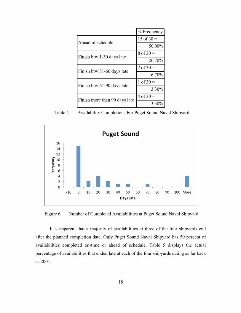
Table 4. Availability Completions For Puget Sound Naval Shipyard

Figure 6. Number of Completed Availabilities at Puget Sound Naval Shipyard

It is apparent that a majority of availabilities at three of the four shipyards end

after the planned completion date. Only Puget Sound Naval Shipyard has 50 percent of

availabilities completed on-time or ahead of schedule. Table 5 displays the actual

percentage of availabilities that ended late at each of the four shipyards dating as far back

as 2001:

19

ShipyardPercentage of

Availabilities thatare Late

Number of Availabilities

Standard Error

Norfolk 55.90% 34 8.50%

Pearl Harbor 82.60% 23 7.90%

Portsmouth 85.70% 21 7.60%

Puget Sound 50.00% 20 11.20% Table 5. Percentage of Completed Availabilities Ended Late from 2001 to 2011

The percentages in Table 5 are associated with the corresponding number of

availabilities shown. Since the percentages are based on a small number of data (only 20

through 34), the standard error of the percentage of availabilities late is shown to provide

an estimate of the possible range of percentages. For example, one could estimate that the

true mean percentage of availabilities that are late at Norfolk Naval Shipyard as between

47.4% and 64.4% (55.9% ± 8.5).

Table 6 (respectively, Table 7) displays the percentage of completed availabilities

that are late for both submarines and carriers. The results suggest that carrier availabilities

typically finish in a more timely manner than submarine availabilities.

ShipyardLate Submarine

Availability Percentage


Standard Error

Norfolk 62.50% 13 13.40%

Pearl Harbor 82.60% 23 7.90%

Portsmouth 85.00% 20 8.00%

Puget Sound 62.50% 16 12.10% Table 6. Percentage of Submarine Availabilities Ended Late per Shipyard

20

ShipyardLate Carrier Availability Percentage


Standard Error

Norfolk 36.40% 11 14.50%

Pearl Harbor N/A 0 N/A

Portsmouth N/A 0 N/A

Puget Sound 30.80% 13 12.80% Table 7. Percentage of Carrier Availabilities Ended Late per Shipyard

These tables raise several questions: “Why are carrier availabilities outperforming

submarine availabilities?” and “Could there be a statistically significant difference

between the performance of Norfolk and Puget Sound and the performance of

Portsmouth and Pearl Harbor in completing submarine availabilities in a timely fashion?”

The percentages and associated standard errors so far do not indicate a statistically

significant difference between the results at the different shipyards. However, there is a

statistically significant difference between the mean late percentages of carrier

availabilities and submarine availabilities. In this context, claiming that the means of two

sets of data are statistically significantly different implies that the two means cannot be

accepted as equal or similar, based on the differences of the means as well as the spread

of the plausible mean values for each data set as illustrated by the standard error. Two

sample t-tests, with the assumption that the means of the two sets of data have unequal

variances, are conducted via computer software such as Microsoft Excel to determine if

the means of two sets of data are statistically significantly different. Additional

information on this approach appears in Section D.

D. COMPARING THE COST PERFORMANCE MEANS

In this section, associations between cost performance, overtime percentage, and

the lateness of the availability are studied. In particular, the possible association between

cost performance (CP = BQWP/AQWP) and overtime percentage (OT%) between

projects ending late and projects ending on-time or ahead of schedule is investigated.

Table 8 displays the descriptive statistics for the four shipyards:

21

Late Not Late Late Not LateMean: 0.87 0.93 Mean: 20.5 20.2StDev: 0.09 0.07 StDev: 6.8 4.8

StError: 0.02 0.02 StError: 0.02 0.01Sample Size: 19 15 Sample Size: 19 15

Mean: 0.83 0.92 Mean: 20 17.7StDev: 0.08 0.08 StDev: 4.1 4.22


Mean: 0.9 1.03 Mean: 20.6 20.3StDev: 0.08 0.14 StDev: 7.4 8.05


Mean: 0.87 0.97 Mean: 19.1 16.1StDev: 0.1 0.06 StDev: 5.4 3.05


Portsmouth Portsmouth

Puget Sound

Puget Sound

CP OT%

Norfolk Norfolk

Pearl Harbor

Pearl Harbor

Table 8. Mean Cost Performances and Overtime Percentages for the Four Shipyards

With this information, a comparison is made between the population means of CP

and OT% for late and timely availabilities across all shipyards with the assumption that

the samples are independent and have unequal variances. The null hypothesis in this

analysis is that the mean CP for late projects equals the mean CP of on-time projects. If

the null hypothesis is rejected, then the alternative hypothesis that there is a statistically

significant difference between the two means is accepted. The t-statistic for the null

hypothesis is computed using equation 1:

2 2( ) ( )meanCPlate meanCPnotlatetStDevLate StDevNotLateSampleSize SampleSize

−=

+

Equation 1. T-statistic to Test Significant Differences between CP Population Means

The t-statistic for the null hypothesis may either fall in the acceptance or rejection

region as determined by the critical t-value tα/2,n-1, where n stands for smaller sample size

of the two populations being compared. The null hypothesis is rejected if |t| > tα/2,n-1

(Hayter 2007). Results are displayed in Table 9 comparing CP and overtime percentages

for all availabilities across all shipyards.

22

CP OT%Mean Late 0.87 0.2Variance Late 0.008 0.004Mean On-Time 0.95 0.18Variance On-Time 0.006 0.002Confidence Level 95% 95%t-statistic 5.28 1.76critical t-value 1.99 1.99P-value 9.70E-07 0.081Reject null? Yes No

Table 9. Results in Testing for Significant Difference of the Means for Cost Performance and Overtime Percentage

Table 9 displays the mean CP and overtime percentage for late and timely

availabilities across the four shipyards. The variance for each value gives an indication of

the spread of the values for each data set. The results suggest that there is a significant

difference between the CP for projects that finish on-time and those that end late. The

results for OT% do not necessarily show conclusive evidence that the means are

significantly different. From this, it is concluded that the overtime percentages for late

and timely availabilities are statistically similar.

E. COST PERFORMANCE GOAL

Availabilities that finish late tend to possess a CP which is less than the CP of on-

schedule availabilities that finish early or on time. The possibility of specifying a CP to

strive for in order to ensure a timely availability is investigated. One-sided t-confidence

intervals are constructed based on the given data sets to determine a lower 99%

confidence bound for the average CP for those availabilities that finished on time or

ahead of schedule and an upper 99% confidence bound for those availabilities that

finished late. The one-sided confidence interval formula appear in equations 2 and 3; µ is

the sample mean and s is the sample standard deviation:

, 1( )_ _ ( , )nt s

Upper confidence boundn

αμ −= −∞ +

23

Equation 2. Upper Confidence Bound for CP of Late Availabilities

, 1( )_ _ ( , )nt s

Lower confidence boundn

αμ −= − ∞

Equation 3. Lower Confidence Bound for CP of Timely Availabilities

The sample means, standard deviations, and sample sizes are computed from the

data sets reflecting all the completed availabilities across the four shipyards and all hull

types. Table 10 displays the descriptive statistics of the data as well as the upper-bound of

the confidence interval for the late availabilities and the lower-bound of the confidence

interval for the on-time availabilities. A confidence level of 99%was used for the

confidence intervals. In addition, the quantiles of the data are displayed to illustrate the

percentage of availabilities with certain CPs.

Mean 0.87 100.00% maximum 1.06Std Dev 0.09 90.00% 1

Std Err Mean 0.01 75.00% quartile 0.93Upper 99% Confidence Bound 0.89 50.00% median 0.87

Num Avails 71 25.00% quartile 0.8110.00% 0.750.00% minimum 0.62

Mean 0.95 100.00% maximum 1.19Std Dev 0.08 90.00% 1.04

Std Err Mean 0.01 75.00% quartile 1.01Lower 99% Confidence Bound 0.92 50.00% median 0.95

Num Avails 37 25.00% quartile 0.8910.00% 0.860.00% minimum 0.83

Cost Performance for Late AvailabilitiesDescriptive Statistics Quantiles

Cost Performance for On-Time AvailabilitiesDescriptive Statistics Quantiles

Table 10. Cost Performance Data Comparison for Late and Timely Availabilities

Figure 7 displays a histogram of the CP ratio for availabilities that finish late and

availabilities that finish early or on time. The results of Table 10 suggest that one could

24

say with 99% confidence that late availabilities will have a mean CP ratio of 0.89 or less

and that on-time availabilities will have a mean CP of 0.92 or higher. However, it appears

that there is a large overlap of CP values among late availabilities and on-time/early

availabilities. Twenty-five percent of late availabilities have a CP ratio of 0.93 or higher,

whereas twenty-five percent of on-time availabilities have a CP ratio of 0.89 or lower.

Although management can strive to ensure a CP ratio of 0.92 or higher, it does not

necessarily guarantee a timely availability.

Figure 7. Frequency of Cost Performance Ratios for Late and Timely Availabilities

E. DAYS LATE VERSUS AVAILABILITY LENGTH

In this section, associations between availability length and the lateness of the

availability are studied. In this case, longer availabilities are availabilities with longer

planned lengths due to the quantity of jobs in the work package and their associated

expected times to completion. The availabilities are arbitrarily partitioned into 3

categories: short with scheduled length less than or equal to 200 days; medium with a

scheduled length between 200 and 400 days; and long with a scheduled length of 400

days or greater. Of the 108 completed availabilities considered, 52 had lengths of 200

days or fewer, 27 had lengths between 200 and 400 days, and 29 had lengths of 400 days

25

or greater. The availabilities consist of various hulls, including carriers, submarines

(SSN, SSBN, and SSGN), as well as Landing Helicopter Dock (LHD) amphibious assault

ships across all four the shipyards. Roughly 70% of the data are from submarine

availabilities and 22% are from carrier availabilities. Table 11 displays the percentage of

availabilities ending on time for each of the three availability length ranges.

0-200 Days 200-400 Days 400+ Days# Availabilities 52 27 29% Late 59.60% 66.70% 75.90%% Late Std Error 6.80% 9.10% 7.90%Mean Length 131 332 694Mean Days Late 44.5 50.2 106Mean Days Late % 42.40% 14.30% 16.70%

Mean Days Late %Standard Error

6.90% 6.70% 6.90%

Availability Length

Table 11. Lateness Statistics of Availabilities of Various Lengths

Table 11 suggests that the longer availabilities are late a greater percentage of the

time than the shorter availabilities, perhaps indicating that larger availabilities have a

greater probability of ending late than shorter ones. However, the standard errors are

large enough to indicate that there is no statistically significant difference between the

percentage of availabilities that are late for each category of availabilities. The row

labeled “mean late %” represents the number of days late as a percentage of the initial

planned length of the availability (for the late availabilities), and it is seen from the table

that, on a percentage basis, shorter availabilities that are late typically have a percentage

of late days far greater than the longer availabilities that are late (42% versus 14% to

16%). A two sample t-test has shown that there is a statistically significant difference in

the ‘mean late %’ for the short availabilities (0–200 days length) and the longer

availabilities. This can be an indication of inaccurate planning for the shorter

availabilities or an inadequate amount of buffer space allowed in the schedule for

unexpected issues, work stoppages, or new work. There is no statistically significant

26

difference in the ‘mean late days %’ for the medium (200–400 day length) and long (400

days or more) availabilities. Table 12 displays summary statistics to consider submarine

availabilities and carrier availabilities separately and the various results based on

availability length.

0-200 Days 200-400 Days 400+ Days# Availabilities 31 15 29% Late 71.00% 80.00% 75.90%% Late Std Error 8.2 10.3 7.9Mean Length 113 356 694StDev Length 33 40 193Mean Days Late 48 62 106Mean DaysLate % 50.70% 17.00% 16.70%

Mean Days Late % Std Error

9 9.7 6.9

0-200 Days 200-400 Days 400+ Days# Availabilities 16 8 0% Late 31.25% 37.50% N/A% Late Std Error 11.6 17.1 N/AMean Length 160 295 N/AStDev Length 38 54 N/AMean Days Late 17 49 N/AMean Days Late % 11.07% 22.80% N/A

Mean Days Late % Std Error

7.8 14.8 N/A

Submarine-only Availability Length

Carrier-only Availability Length

Table 12. Lateness Statistics of Submarine and Carrier Availabilities of Various

Lengths

When the data are summarized by the number of days late as a percentage of

availability planned length, submarine projects between 0 and 200 days have a mean

percentage that is substantially higher than the mean percentage of days late for longer

submarine projects. The following plot may offer a better illustration of availability

length on days late as a percentage of planned length.

27

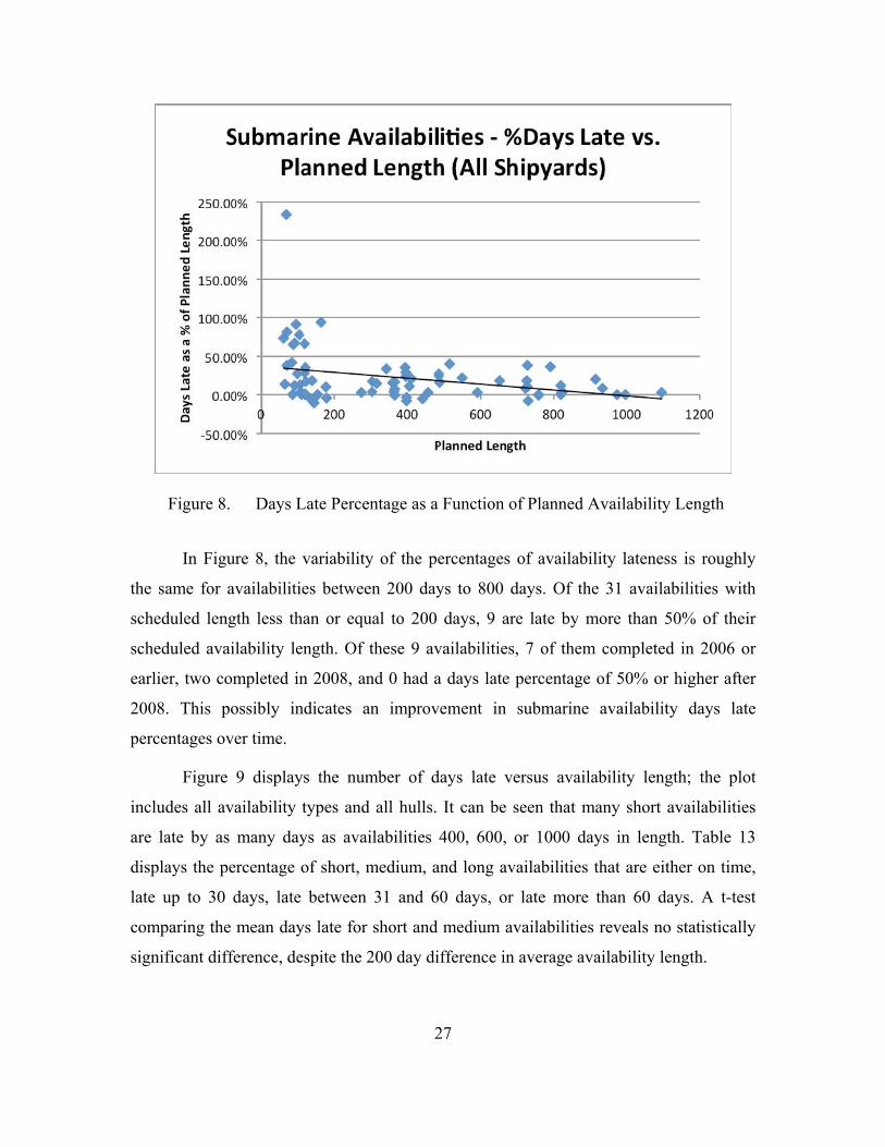
Figure 8. Days Late Percentage as a Function of Planned Availability Length

In Figure 8, the variability of the percentages of availability lateness is roughly

the same for availabilities between 200 days to 800 days. Of the 31 availabilities with

scheduled length less than or equal to 200 days, 9 are late by more than 50% of their

scheduled availability length. Of these 9 availabilities, 7 of them completed in 2006 or

earlier, two completed in 2008, and 0 had a days late percentage of 50% or higher after

2008. This possibly indicates an improvement in submarine availability days late

percentages over time.

Figure 9 displays the number of days late versus availability length; the plot

includes all availability types and all hulls. It can be seen that many short availabilities

are late by as many days as availabilities 400, 600, or 1000 days in length. Table 13

displays the percentage of short, medium, and long availabilities that are either on time,

late up to 30 days, late between 31 and 60 days, or late more than 60 days. A t-test

comparing the mean days late for short and medium availabilities reveals no statistically

significant difference, despite the 200 day difference in average availability length.

28

<= 0 21 40.40% 6.80%1 to 30 15 28.80% 6.30%

31 to 60 9 17.30% 5.20%60+ 7 13.50% 4.70%

<= 0 9 33.30% 9.10%1 to 30 8 29.60% 8.80%

31 to 60 5 18.50% 7.50%60+ 5 18.50% 7.50%

<= 0 7 24.10% 7.90%1 to 30 3 10.30% 5.70%

31 to 60 3 10.30% 5.70%60+ 16 55.20% 9.20%

Days LateNumber of

AvailabilitiesPercentage of

TotalStandard Error of

Percentage

Short Availabilities (0 to 200 days in length)

Days LateNumber of



Percentage

Medium Availabilities (200 to 400 days in length)

Days LateNumber of



Percentage

Long Availabilities (400+ days in length)

Table 13. Lateness Frequencies of Availabilities of Various Lengths

Figure 9. Number of Days Late as a Function of Planned Availability Length

29

F. NUMBER OF AVAILABILITIES IN THE SHIPYARD VERSUS THE NUMBER OF DAYS LATE AS A PERCENTAGE OF PLANNED AVAILABILITY LENGTH

In this subsection, associations between number of availabilities being conducted

in a yard and availability lateness is studied. For instance, availabilities may be more

likely to be late and have a greater number of days late as a percentage of planned length

if there are a total of 8 availabilities going on at the shipyard, causing the shipyard to use

more of its resources and to operate at close to maximum capacity as opposed to

operating at 50% capacity with only 4 availabilities underway. Gantt charts are

constructed for each of the four shipyards illustrating the historical schedule of all the

availabilities that took place in each shipyard dating as far back as 2001 and extending all

the way to as recent as 2011. The Gantt charts are effective in showing the number of

total availabilities as well as the different kinds of vessels being worked on across certain

time periods. Figure 10 displays the Gantt chart for data from Norfolk Naval Shipyard

between 2005 and 2009.

30

Figure 10. Availabilities in Norfolk Naval Shipyard between 2005 and 2009

In Figure 10, the blue bars represent submarine availabilities, the red represent

carrier availabilities, the green represent LHD availabilities, the purple represent MTS

availabilities, and the yellow represents an AS availability. The start and finish dates of

the corresponding availabilities are given in the columns labeled ‘Start’ and ‘Finish.’

Even though data for availabilities starting as early as 2003 and ending as late as 2011 are

available, the time range of 2005 to 2009 is studied to ensure all the availabilities that

occurred during those years are included.

31

There are certain time periods where more projects are underway than in others.

Using the Gantt chart of Norfolk in Figure 10, one can see that there were only three

projects underway in Quarters 2 and 3 of 2006 whereas in Quarters 2 and 3 of 2007 there

are six and in Quarters 1 and 2 of 2008 there were as many as eight projects underway.

To study possible associations between availability lateness and the number of ongoing

projects, the number of availabilities that were underway is counted in the shipyard each

year from 2005 to 2009. It is assumed that an availability that is underway for a minimum

of 3 months during a year may have an impact on other availabilities being conducted

during that year. Thus, if an availability ended in February of 2005 as in the case of the

depot modernization period for the USS Boise (BBE), it was not counted towards the

total number of availabilities underway in 2005. The next step averages the days late as a

percentage of the planned length of the availability of the availabilities that were

underway for at least 3 months for each year. The percentage figures next to each color

coded bar in the Gantt chart above represent the days late as a percentage of the planned

length of the availability. As an example using the Norfolk Gantt chart displayed in

Figure 10, seven total availabilities were counted for 2005: FLA, PRT, HPN, GRG,

NEW, ENW, and CHR. Their corresponding days late percentages are then averaged, as

displayed in Equation 4.

0% 16.44% 11.08% 8.77% 41.47% 0% 39.65% 16.8%7Availabilities

+ + + + + +=

Equation 4. Sample Calculation of Mean Days Late Percentage for Availabilities

Underway Simultaneously in a Shipyard

Table 14 displays the percentage of availabilities that are late as well as the average

number of days late as a percentage of scheduled availability length (Mean Days Late %)

for the years 2005 to 2009 for each of the four shipyards.

32

2005 7 486.1 85.70% 16.80% 14.10%2006 6 581 66.70% 11.30% 12.90%2007 8 467.3 62.50% 13.00% 11.90%2008 9 315.1 66.70% 8.40% 9.20%2009 7 301.2 50.00% 4.00% 7.40%

2005 5 291 100.00% 60.70% 21.80%2006 6 387.5 83.30% 27.60% 18.20%2007 3 451.7 66.70% 6.20% 13.90%2008 6 429.7 66.70% 8.70% 11.50%2009 5 499 80.00% 13.10% 15.10%

2005 4 516 100.00% 19.40% 19.80%2006 5 474.2 100.00% 19.10% 17.60%2007 6 341.8 100.00% 28.10% 18.30%2008 7 399.7 100.00% 18.50% 14.70%2009 6 433.5 83.30% 9.50% 12.00%

2005 4 797.3 25.00% 0.80% 4.60%2006 7 445.6 57.10% 19.50% 15.00%2007 7 422.1 57.10% 12.70% 12.60%2008 7 505.9 28.60% 3.10% 6.60%2009 4 478.5 25.00% 4.60% 10.50%

Puget SoundNumber of

AvailabilitiesMean

Length% Late Mean Days

Late %Std Error

PortsmouthNumber of

AvailabilitiesMean


Late %Std Error

Pearl HarborNumber of

AvailabilitiesMean


Late %Std Error

NorfolkNumber of

AvailabilitiesMean


Late %Std Error

Table 14. Days Late Percentage Statistics with Various Amounts of Availabilities

Underway in the Shipyard

The summary statistics in Table 14 suggest no clear association between the

number of availabilities underway in the yard and the mean days-late percentage. In the

case of Portsmouth, there are six availabilities underway for a majority of 2007 and 2009,

but the mean of the days-late percentages are 28.1% and 9.5%, respectively. For

Portsmouth, there does not seem to be much difference between the days late percentage

of those availabilities in 2005 when only four are underway and those in 2008 when

seven are underway. Figure 11 displays data from Table 14.

33

Figure 11. Days Late Percentage as a Function of the Number of Availabilities Underway in the Shipyard

The data displayed in Figure 11 does not suggest a simple relationship between

the percentage of days late and the number of availabilities in the yard. The greatest days

late percentage for Pearl Harbor occurs with five availabilities underway simultaneously

as compared to four or six. The greatest percentage of days late for Norfolk occurs with

seven availabilities in the yard as compared to six or nine, and Portsmouth has the

greatest percentage of days late with six availabilities in yard as compared to four or

seven. Further investigation of any differences between shipyard managerial practices or

availability planning methods that may exist with differing numbers of availabilities in

the shipyard can lead to increased knowledge of the reasons behind availability lateness.

However, taking the standard errors of mean days late percentages into consideration, one

can conclude that there is no statistically significant difference between the percentage of

days late with regard to the number of availabilities in the shipyard.

Something that stands out from the data summaries displayed in Table 14 is the

general improvement in the percentage of days late performance across all the four

shipyards from 2005 to 2009. By simply observing the days-late metric across these

years, the

34

days late percentage has been decreasing. Figure 12 displays the days-late percentage as a

function of year. The dotted lines represent one standard error about the mean for Pearl

Harbor and Puget Sound.

Figure 12. Days Late Percentage Trends from 2005 to 2009

With the exception of 2005, the performance of each shipyard is similar for the

years 2006 to 2009. The small number of availabilities considered result in large standard

errors for the mean days late percentage; there is no statistically significant difference in

the days late percentage between the shipyards between 2006 and 2009. Also, it appears

that the mean days late percentage across all shipyards is trending downwards from year

to year after 2006. Because of this, it is of interest to see how the days late percentage of

availabilities changes from year to year across all shipyards beyond the 2005 to 2009

period. Table 15 displays the mean days-late percentage of all the availabilities that were

underway in three separate periods: 2005 and earlier, 2006–2008, and 2009–2010.

35

2003 to 2005 2006 to 2008 2009 to 2011

# Availabilities 8 14 12

Mean Days Late % 8.10% 9.90% 11.90%

Std Error 5.40% 3.60% 5.70%

2003 to 2005 2006 to 2008 2009 to 2011


Mean Days Late % 79.20% 16.10% 9.70%

Std Error 24.70% 7.30% 3.90%

2003 to 2005 2006 to 2008 2009 to 2011


Mean Days Late % 12.20% 28.60% 7.30%

Std Error 7.40% 8.20% 7.20%

2002 to 2005 2006 to 2008 2009 to 2011


Mean Days Late % 10.10% 14.20% 5.10%

Std Error 5.90% 7.10% 3.30%

Norfolk

Pearl Harbor

Portsmouth

Puget Sound

Table 15. Lateness Statistics over Time

Table 15 displays the number of availabilities underway in each of the associated

time periods, along with the mean days late as a percentage of planned length and

associated standard errors for those availabilities. For an availability to be associated with

the 2003 to 2005 time period, a majority of the availability had to take place in that time

period. For example, if an availability spanned from May of 2005 until March of 2006, it

36

was associated with the 2003 to 2005 time period because the availability took place for

eight months in 2005 and only 3 months in 2006. Figure 13 displays the data in the

Table 15.

Figure 13. Days Late Percentage Trends from 2003 to 2011

It can be seen that Pearl Harbor shows a continual improvement in the percentage

of days late of its availabilities over the three time periods, whereas Norfolk shows a

nearly consistent percentage of days late. Even if one availability skews the mean

percentage values, as in the case of Norfolk’s performance in 2009 through 2011 where

one availability conducted on an MTS with a percentage of days late of 62% skewed the

average higher, the assumption that all availabilities within a shipyard are interdependent

means that the averages properly reflect the performance of the shipyards during that

time period. Since Portsmouth and Puget Sound also show improvement in 2009 through

2011 over the 2006 through 2008 periods; although with large associated standard errors,

it is possible that the mean percentage of days late of availabilities in general have been

decreasing after 2006.

37

G. EFFECTS OF WINTER MONTHS ON AVAILABILITY LATENESS

In this subsection, associations between the times of year an availability is

conducted in Puget Sound and Portsmouth and the number of days late is investigated; in

particular it is of interest to investigate possible associations between average percentage

of days late and number of months an availability is conducted during the winter months

for Puget Sound and Portsmouth. For completed availabilities dating back to 2002, the

amount of time the availability is conducted in the winter months as a percentage of the

entire length of the availability is calculated and then plotted against the availability’s

associated days late as a percentage of planned length. The initial hypothesis is that the

greater the percentage of time conducted during the winter months, the greater the

number of days late as a percentage of the availability length. The months associated with

the most extreme weather in Portsmouth are assumed to be December through April

because this is the time period when the Portsmouth, New Hampshire/Kittery, Maine area

would typically experience the most snowfall (8–12 inches per month December through

March) and rainfall (over 9 inches in April, which is 2–3 times more than any other

month during the year). The months associated with the most extreme weather in Puget

Sound are assumed to be November through March. The Bremerton, Washington area

does not typically experience great amounts of snowfall, however it is during these

months where there is the greatest amounts of rainfall as compared to the rest of the year.

Figure 14 and 15 display the results obtained for submarine availabilities.

38

Figure 14. Days Late Percentage as a Function of Percentage of Availability Duration in Inclement Weather Months at Puget Sound Naval Shipyard

Figure 15. Days Late Percentage as a Function of Percentage of Availability Duration

in Inclement Weather Months at Portsmouth Naval Shipyard

In the case of Puget Sound, there may be some association between the amount of

time spent in the winter months and the number of days late as a percentage of

39

availability length. 25% of the availabilities with 30% to 40% of time conducted in the

winter months had a days late percentage of 20% or more. Over 28% of the availabilities

(2 of 7) with a 40% to 50% percentage of time conducted in winter had a days late

percentage of 20% or more. Also, of all the availabilities where less than 30% of time

was spent during the winter months, none had greater than 20% days late as a percentage

of planned length. In the case of Portsmouth, there does not seem to be as clear an

association between the amount of time an availability is conducted in the winter months

and the days late percentage. Portsmouth has an example of an availability with no time

spent in the winter months but still having a number of days late that is roughly 65% the

length of the original planned length.

H. IMPACT OF CARRIER AVAILABILITIES ON SUBMARINE AVAILABILITIES

It has been speculated among subject-matter experts that carrier availabilities take

precedence over submarine availabilities when it comes to timely maintenance project

completion. This is due to a fewer number of carriers and the fact that carrier

maintenance can impact the operational schedules of entire carrier battle groups. A

hypothesis is that carrier availabilities may draw on manpower resources available from

submarine availabilities in order to ensure timely completion. If this is the case, it would

be interesting to study on a case by case basis the days late percentage of a submarine

availability as a function of the number of carrier availabilities underway during the

submarine’s availability schedule. Data from fifteen submarine availabilities at Puget

Sound are examined to determine the duration that either one or two other carrier

availabilities were underway as a percentage of the total length of the submarine

availability. For example, if a submarine availability lasts 200 days, and during 30 days

of that time period two other carrier availabilities were being conducted and during 100

days only one other carrier availability was being conducted, then for 15% of the

availability (30/200) two other carrier projects were being conducted and for 50% of the

availability (100/200) only one other carrier project was being conducted. Each of the

fifteen submarine availabilities are assigned a carrier impact factor which was calculated

by multiplying 2 by the percentage of time that two carriers availabilities were underway

40

during the submarine’s availability and adding to that the percentage of time that only

one carrier was underway during the submarine’s availability. Equation 5 displays the

calculation for this example.

(2x15%) + (50%) = 80 Carrier Impact Factor

Equation 5. Sample Calculation for Carrier Impact Factor

The carrier impact factor for each availability is then compared to the submarine

availability’s number of days late as a percentage of planned availability length to

investigate whether a larger carrier impact factor would result in a larger days late

percentage. Table 16 and Figure 16 display the carrier impact factors and corresponding

percentage of days late as a percentage of planned length for the submarine availabilities

that occurred in Puget Sound shipyard between 2001 and 2011.

USS HOUSTON (SSN 713) 7/8/04 730 48.1 38.49%

USS OHIO (SSGN 726) 12/23/05 1096 72.7 3.47%

USS JEFFERSON CITY (SSN 759) 8/1/04 394 91.2 35.28%

USS MICHIGAN (SSGN 727) 12/6/06 996 81.6 0.00%

USS COLUMBUS (SSN 762) 12/16/06 760 82.1 -0.13%

USS ALABAMA (SSBN 731) 5/16/08 821 100.2 3.41%

USS HELENA (SSN 725) 5/27/06 60 83.7 73.33%

USS TOPEKA (SSN 754) 11/20/06 107 98.2 3.74%

USS HONOLULU (SSN 718) 11/30/08 760 102.2 0.00%

USS SAN FRANCISCO (SSN 711) 4/14/09 727 99.6 18.43%

USS ASHEVILLE (SSN 758) 9/11/07 91 129.3 12.09%

USS NEVADA (SSBN 733) 5/7/10 820 78 0.00%

USS JIMMY CARTER (SSN 23) 7/3/08 120 34.2 0.00%

USS JEFFERSON CITY (SSN 759) 12/20/08 110 100 0.00%

USS JIMMY CARTER (SSN 23) 12/23/10 303 87.3 3.63%

Puget Sound Naval Shipyard

Availability End DatePlanned Length (Days)

Carrier Impact Factor

Days Late Percentage

Table 16. Carrier Impact Factors and Submarine Availability Lateness Statistics at

Puget Sound Naval Shipyard

41

Figure 16. Days Late Percentage as a Function of Carrier Impact Factor

This plot does not provide clear evidence that carrier availabilities have a direct

association with the lateness of submarine availabilities based on fifteen data samples.

Further investigation can include a similar study of the submarine availabilities at

Norfolk Naval Shipyard. Pearl Harbor and Portsmouth shipyards do not conduct carrier

availabilities. Figure 17 displays the carrier impact factor as a function of availability

length, which demonstrates clearly that longer availabilities do not have a tendency to

negatively impact carrier availabilities.

42

Figure 17. Carrier Impact Factor as a Function of Planned Availability Length

I. IMPACT OF PERSONNEL RESOURCES ON AVAILABILITY LATENESS

In this subsection, the relationship between the number of personnel resources

available to work on an availability (measured in average man-days per month), with

availability lateness is studied. The data provide values for BQWP, AQWP, availability

start dates, availability end dates, and finally, the number of days the availability

completes late. Two estimates are calculated for comparison: the planned number of

man-days required to complete the work for each availability per month (BQWP/mo) and

the actual number of man-days charged to each availability per month (AQWP/mo). The

estimated planned number of man-days per month is calculated by dividing the BQWP

by the planned availability length in months. The estimated actual number of man-days is

calculated by dividing AQWP by the actual availability length in months. To determine

actual availability lengths, the number of days between availability start and end is

calculated and then divided by 30.42, which is the average number of days per month

over a given year (365/12 = 30.42). Planned availability length is calculated as the

number of actual days between start and end minus the number of days late and divided

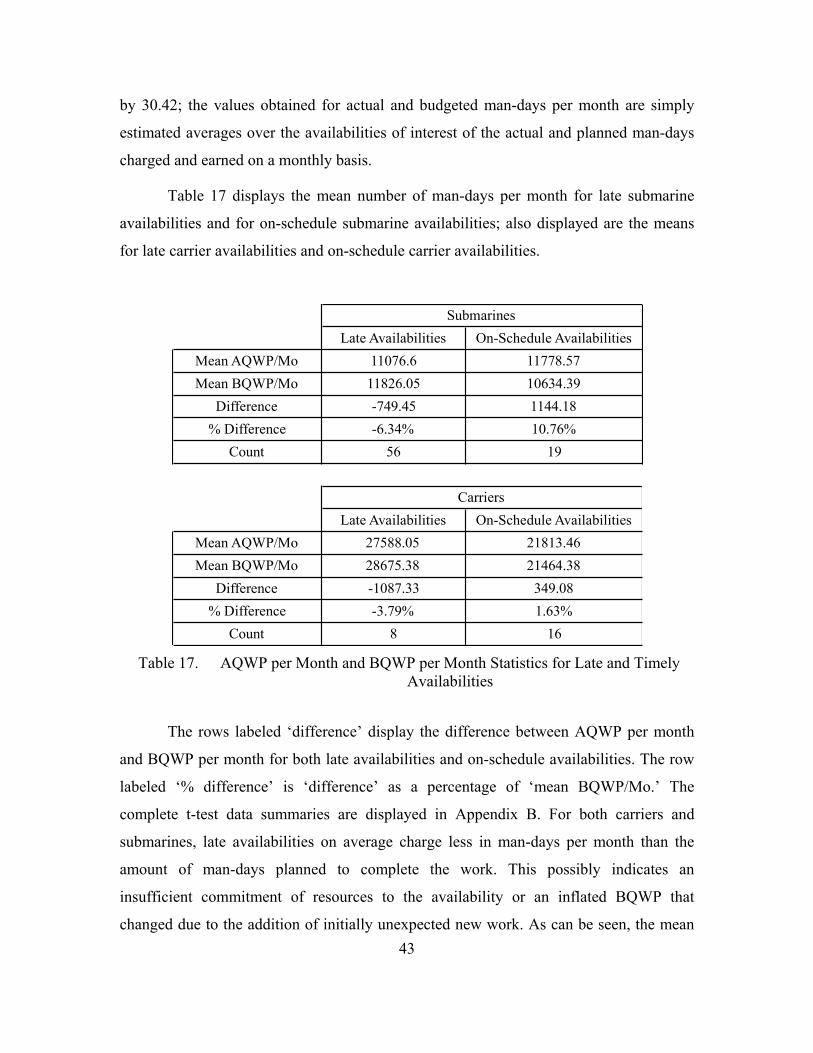
43

by 30.42; the values obtained for actual and budgeted man-days per month are simply

estimated averages over the availabilities of interest of the actual and planned man-days

charged and earned on a monthly basis.

Table 17 displays the mean number of man-days per month for late submarine

availabilities and for on-schedule submarine availabilities; also displayed are the means

for late carrier availabilities and on-schedule carrier availabilities.

Late Availabilities On-Schedule AvailabilitiesMean AQWP/Mo 11076.6 11778.57Mean BQWP/Mo 11826.05 10634.39

Difference -749.45 1144.18% Difference -6.34% 10.76%

Count 56 19


Difference -1087.33 349.08% Difference -3.79% 1.63%

Count 8 16

Submarines

Carriers

Table 17. AQWP per Month and BQWP per Month Statistics for Late and Timely

Availabilities

The rows labeled ‘difference’ display the difference between AQWP per month

and BQWP per month for both late availabilities and on-schedule availabilities. The row

labeled ‘% difference’ is ‘difference’ as a percentage of ‘mean BQWP/Mo.’ The

complete t-test data summaries are displayed in Appendix B. For both carriers and

submarines, late availabilities on average charge less in man-days per month than the

amount of man-days planned to complete the work. This possibly indicates an

insufficient commitment of resources to the availability or an inflated BQWP that

changed due to the addition of initially unexpected new work. As can be seen, the mean

44

BQWP per month for timely availabilities of both carriers and submarines tends to be less

than the mean BQWP per month for late availabilities. Also important to note is that the

charged amount of work per month for timely availabilities tends to exceed the planned

amount of work per month, possibly indicating a commitment of a greater magnitude of

resources to the project to ensure timeliness. To investigate further, late and on-schedule

availabilities were broken down by availability type to ensure that similar availabilities

are being compared.


Difference -2112.75 866.87% Difference -18.14% 8.68%Num Avails 20 7

Submarine DSRA (SSN)



Submarine DMP (SSN)


Difference 10.83 530.96% Difference 0.22% 11.62%Num Avails 3 3

Submarine IA (SSN)


Difference 910.89 907.37% Difference 6.25% 6.34%Num Avails 4 3

Submarine ERO (SSBN/SSGN)

Table 18. AQWP per Month and BQWP per Month Statistics for Various

Availability Types

45



CARRIER PIA (CVN)

Table 19. AQWP per Month and BQWP per Month Statistics for Various Availability

Types

The statistics in Table 19 (standard errors of the means are displayed in

Appendix C) suggest that for all availability types, the mean AQWP per month tends to

exceed the planned BQWP per month for timely availabilities. The statistics also suggest

that for all availability types, with the exception of SSBN/SSGN engineering overhauls

and SSN inactivation activities, the mean AQWP per month tends to be less than the

planned BQWP per month for late availabilities, although the figures for overhauls and

IAs are similar. Additionally, for all availability types, the average amount of resources

needed to complete the work as represented by BQWP per month tends to be greater for

late availabilities than timely availabilities.

Taking on a different perspective will shed some light on the amount of personnel

resources needed on a monthly basis to ensure a timely availability. In this summary,

both the AQWP and BQWP of the availability are divided by the planned availability

length in months. If the actual quantity of work performed is divided by the planned

length, this can give an indication of the amount of work that would have been required

on a monthly basis to finish the availability by the planned end date. Table 20 displays

the results.

46

Late Availabilities On-Schedule AvailabilitiesMean AQWP 14045.9 11493.6Mean BQWP 11826.1 10634.4

Difference 2219.8 859.2% Difference 18.77% 8.08%

Count 56 19

Late Availabilities On-Schedule AvailabilitiesMean AQWP 31702.5 21727.4Mean BQWP 28675.4 21464.4

Difference 3027.1 263% Difference 10.56% 1.23%

Count 8 16

Submarines

Carriers

Table 20. AQWP and BQWP divided by Planned Availability Length in Months

For both late submarine and carrier availabilities, the actual average quantity of

work performed per month is greater than the budgeted quantity of work performed per

month by roughly 18% and 10% of the planned work, respectively. The on-schedule

availabilities show a closer match between the man-days charged on a monthly basis and

the planned number of monthly man-days needed. In conclusion, the monthly average

man-days required to complete the availability tends to be greater than the planned

monthly average by a larger amount for late availabilities than for timely availabilities.

J. SUMMARY

Shipyard performance data are summarized and displayed in various ways to gain

insight into possible reasons contributing to availability lateness. The study is limited to

data on 108 completed availabilities, resulting in a limited ability to produce statistically

significant conclusions. The sections to follow analyze the impacts of a factor not yet

covered in this study: work stoppages.

47

IV. AVAILABILITY EXECUTION

A. INTRODUCTION

This chapter summarizes the theory on network scheduling, describes work

stoppages, and provides background information on availability execution processes. The

intent of this chapter is to describe how work stoppages influence the execution of an

availability.

B. NETWORK SCHEDULING

Shipyard project managers continually track and update all in-progress jobs

during an ongoing availability, with the goal of finishing the availability on time. The

scheduling (planning phase) and maintaining (execution phase) of the Availability Work

Package (AWP, discussed in Chapter II) jobs is one of the most important activities to

accomplish in the determination of how an availability’s resources should be integrated,

especially when multiple jobs during a single availability are executing in parallel

(Kerzner 2009). Due to the high complexity of the AWP and tight schedule deadlines,

project managers are challenged to solve problems rapidly, efficiently, and with minimal

impact to separate on-going jobs. As a result, scheduling techniques have been developed

which allow project managers to mitigate the effects of unplanned events that arise

during availability execution. Network modeling and critical path analysis are essential

for project managers to understand in order to reveal the interdependencies between the

on-going jobs and to help managers evaluate alternatives by answering questions such as

how time delays will affect the availability’s completion (2009).

1. Network Fundamentals

A project is composed of a series of activities, determined by the management

team, and constructed in such a way to achieve a desired objective (Blanchard and

Fabrycky 2011). A network diagram is a pictorial representation of the events and

activities that must be accomplished for a project to be deemed complete. Applying this

definition and terminology to a CNO availability, events are the major milestones of the

availability, for example, start availability (denoted SA00), complete undocking (denoted

48

UD00), and complete availability (denoted CA00). Network activities are the work

package jobs, for example, engine clean and inspection, compartment painting, and fire

pump maintenance. The construction of a network diagram allows the availability’s

management team to identify all interdependencies that are present between events and

activities (Kerzner 2009).

As seen in Figure 18 of a network diagram, each activity consumes time and is

represented by a single box. Activities are linked in a precedential order in order to show

which activities must be finished before others can start. The arrows show activity

precedence, and an activity is unable to start until all prior activities linked to it by the

arrows are finished (2009). Each box is assigned a unique activity number, located at the

lower left hand corner, which signifies precedence level.

Figure 18. Network Diagram Example (After Langford 2011)

49

All activities are assigned durations by estimating how long each activity will

take, to include the time for all work to be completed plus preparation and waiting time.

Realistic durations are essential to developing a credible, executable availability

schedule. Work package job durations must be determined in a judicious, carefully

considered manner. Job duration estimation reflects the manner in which the work will be

performed as well as the historical performance of similar work (“Baseline Project

Management Plan,” NAVSEA 07, 2009). The next step after duration estimation is to

calculate the project schedule that provides the earliest and latest times at which each

activity can start and finish. The earliest start time for an activity is based on the

projected estimated start time and the duration estimation for preceding activities.

Likewise, the earliest finish time is calculated by adding the given activity’s duration to

the activity’s earliest start time (Kerzner 2009). The latest start and finish times is a

backwards calculation, starting from the completion date, with the intention of

determining the latest time at which an activity can take place without extending the

completion date of the project (2009). The difference between the scheduled completion

date and the total duration date is known as the slack time, commonly referred to as

“float” in the Naval project management community.

a. Float

Float is an important measurement that allows an availability’s

management team to determine how early or late an activity can start or finish. Float, as

mentioned earlier, is the difference between the latest finish date and the earliest finish

date. This difference will indicate whether the project will need to be accelerated or not,

based on the three types of float, described as follows:

• Positive float is the maximum amount of time the activities on the critical path can be delayed without jeopardizing the project’s completion date.

• Negative float is the amount of time the activities on the critical path must be accelerated in order to meet the project’s completion date.

• Zero float means the critical path does not need to be accelerated, nor can it be delayed (Langford 2011).

50

Float during a CNO availability is calculated on multiple levels: each job,

each important milestone, and the availability completion’s float are all calculated.

Negative float occurs when the planned or actual duration of the project extends beyond

the planned end date. Negative float during the planning phase of an availability may

signify an unreasonable amount of work is scheduled for the time allotted. Positive float

experienced during the planning phase but negative float experienced during the

execution phase can be attributed to job duration estimations and planned completion

dates being highly optimistic and unrealistic (Kerzner 2009). NAVSEA currently directs

all availability planning teams to add 30 extra days to the availability completion date to

ensure that positive float is maintained during the availability’s execution (“AIM-NG

Process Manual,” NAVSEA 04X, 2009).

2. Scheduling Problems

Problems arise during the execution of all availabilities that can impact the

schedule by decreasing the amount of float. Scheduling problems include (but are not

limited to) using unrealistic estimates for job durations, lack of personnel with requisite

skills, over committing resources and having to share critical resources across several

projects, frequent revisions to the primary work schedule, and unforeseen bottlenecks

(Kerzner 2009). An availability work stoppage is a type of schedule problem and it is the

primary factor that this research considers. The Theory of Constraints, which is a

schedule improvement methodology discussed in the next section is applied to the

availability work stoppage data in order to identify the impact on schedules due to work

stoppages.

C. THEORY OF CONSTRAINTS

The Theory of Constraints (TOC) is the management technique, introduced by

Eliyahu M. Goldratt, which seeks to improve the process of planning and execution. In

Thomas B. McMullen’s 1998 book, Introduction to the Theory of Constraints

Management System, he states, “the Theory of Constraints always ask, ‘What must

something be if, in its category, it is inevitably to be the best that can be?’” TOC is

applied using the proposed five-step process:

51

1. Identify the system’s constraints.

2. Decide how to exploit the constraints.

3. Fully support the decision by means of policies, processes, and resources.

4. Remove the identified constraints.

5. Return to Step 1.

McMullen further discusses that regardless of the system, to which TOC is being

applied, it is assumed that in order for TOC to be effective, the system must have a goal.

The goal of the system has three requirements: its owners must determine the goal; it

must be measureable; and it is subject to necessary conditions. In the case of a shipyard

availability, the owners are the stakeholders, which include the availability’s planning

and execution teams, the shipyard’s leadership, and NAVSEA. The measureable goal is

to maintain and stay-on schedule. The third requirement, necessary conditions, is the

procedures and laws of the shipyard that ensure the continuing operation of the

availability. Examples of conditions include the shipyard safety requirements, technician

qualifications, and workmanship quality. The primary goal of NAVSEA with respect to

maintenance activities, regardless of system application, is in developing, delivering, and

maintaining ships and systems on time and on cost for the United States Navy. Within the

scope of TOC and this thesis, the NAVSEA goals, according to NAVSEA’s Strategic

Business Plan for 2009–2013, are identified as follows:

• Develop annual balanced, optimized, and integrated Maintenance and Modernization Execution Plans for shipyards.

• Execute the Maintenance and Modernization Execution Plan and assess the results using metrics.

Based on these specified NAVSEA goals, this thesis’ work stoppage analysis

assumes that the primary goal of a shipyard availability is to complete the AWP on time,

according to the planned schedule. This goal is applied to the availability as a whole and

also to individual jobs themselves. It is further assumed that work stoppages are the TOC

quantitative measurements used to determine a schedule constraint.

A constraint is defined as anything that blocks the system from accomplishing its

goal (McMullen 1998). During the execution phase of an availability, work package jobs

52

are started as dictated by the project schedule and the project manager. Once the job is

started, it is classified as an active job and it is assumed that the job will finish on time

and in the correct manner. If during the execution of an active job, a constraint is

identified which prevents the job from being accomplished on schedule, a work stoppage

is activated. The work stoppage is not closed until the constraint is resolved and work on

the job is resumed. Constraints are organized into two categories: physical and policy.

Physical constraints are classified as “scarce resources” whereas a policy constraint

contains all other types of constraints. Work stoppages are classified based on eight

categories, known as reasons. Table 20 organizes the work stoppage reasons by constraint

type (1998):

Physical Constraint Policy Constraint

Material Technical Direction

Labor Resources Work Control

Tooling Workmanship/Rework

Interference/Coordination

Safety

Table 21. Work Stoppage Reasons Organized Based on Constraint Type

1. Critical Chain Management

Critical chain management is a methodology that addresses the need to get each

project completed quickly and funnel more projects through the organization without

additional resources (Kerzner 2009). A critical chain is defined as the longest chain of

dependent events and/or activities where the dependency is either task or resource

related. It is assumed from this definition that the longest chain of a project is most likely

to negatively impact the overall duration of a project (2009). Stepping back to network

fundamentals, a project’s network diagram is composed of activities in multiple parallel

and series configurations, being executed simultaneously; all the paths of activities need

53

to be completed according to the schedule. Project managers rely on critical chain

management to prioritize jobs and focus on the most crucial path of activities to be

completed. The critical chain is the most time consuming path of activities during

execution and is depicted as the longest path of activities in the network diagram; an

example is displayed in Figure 19.

TOC is used to specify the critical path (chain) of sequential jobs whose late

completion most adversely affects the timely completion of the availability. The

NAVSEA WebAIM-NG software assists the availability’s project manager in managing

unexpected delays, in order to keep the critical path’s work progressing.

Figure 19. Critical Chain Colored in Red (After Langford 2011)

D. WORK STOPPAGE

The term “work stoppage” is defined as a delay experienced by a job during the

execution phase of the availability. Specifically, a work stoppage occurs when work on a

54

job is delayed by more than one shift (“AIM-NG Process Manual,” NAVSEA 04X,

2009). Work stoppages are categorized into eight reason codes (RSN):

• Technical Direction (TD)–awaiting engineering resolution or technical direction (i.e., NAVSEA approved instructions) for work continuation.

• Material (MAT)–delay in obtaining/receiving material.

• Tooling (TL)–delay due to limited quantity of tools and manufacturing support of new special tooling.

• Labor Resources (RSC)–shortage of manpower and other support services.

• Work Control (WC)–administrative controls over system conditions needed to ensure safe work conditions are met prior to start of work

• Workmanship/Rework (W)–delay due to rework

• Interference/Coordination (IC)–delay due to multi-job priority levels, often due to space constraints and conditions.

• Safety (SAF) –delay due to shipyard safety violation

E. WEB AIM-NG SOFTWARE

WebAIM-NG software is a project management tool, utilized for both planning

and executing an availability, which assists the availability project team in planning,

monitoring, and tracking all AWP jobs. This section describes the role of the software in

the execution of shipyard availabilities.

1. Execution Priorities

Execution Priorities (EPR), as described in the AIM-NG Process Manual, is a

logic process within the WebAIM software that develops and establishes shipyard

priorities across all projects and availabilities within each shipyard. One of the main

objectives of the EPR process is to identify on a daily basis the jobs that must be

supported to maintain the non-stop execution of the critical chain in each availability.

EPR tracks all activities and analyzes their impacts to the schedule. This is accomplished

by evaluating activity durations, resource requirements, network sequencing, and known

constraints in order to continually develop a list of priorities to aid the program manager

in establishing a path forward. Figure 20 represents the EPR process and describes the

required inputs, process logics, and the resulting outcomes. Depending in the daily

55

impacts and the continual evaluation and identification of critical jobs by the EPR, the

availability may have a continually changing critical path.

Figure 20. EPR Process Diagram (After NAVSEA 04X 2009)

EPR color-codes all activities in order to bring attention to the critical work,

prioritizing based on each activity’s float, according to the following:

• Red activities have fewer than 10 shifts of float and are on or near the Critical Chain. Completing Red activities late will likely prevent the project from meeting the key event associated with the activity.

• Yellow activities are the next-most-important selection of activities relative to completing events.

• Green activities more than 30 shifts of float.

The color-coded activities are compiled and distributed into the Daily Priority List

(DPL). The DPL lists the activities in priority number order, with the most critical

activity needing support first. Availability teams use the DPL on a daily basis to identify

the critical problems and develop/implement corrective actions with the goal of ensuring

timely completion of work on of the critical chain.

56

F. SUMMARY

Network models are the framework for the management of the availability

execution process. By identifying the interdependencies between project activities,

network models allow for the identification of the critical chain. As the longest chain, in

terms of completion time, of connecting activities, the time to complete the jobs in the

critical chain can impact the overall duration of the entire project. Due to the importance

of this crucial chain of activities and the high complexity level of a shipyard availability,

shipyards employ the WebAIM-NG software, which aids the availability team in

identifying the critical chain and allows the team to support timely work completion of

activities on this chain.

57

V. WORK STOPPAGE ANALYSIS

A. INTRODUCTION

This chapter displays statistical summaries of work stoppage data. The goal of

this analytical chapter is to summarize the work stoppage data to display commonalities

between availabilities and to investigate possible trends in work stoppages and predictors

of availability lateness. In order to identify associations between work stoppages and

availability lateness, the analysis assumes that work stoppages are the only reason for

schedule delays; no other factors and influences are considered.

B. RAW WORK STOPPAGE DATA

Work stoppage data are provided, in Microsoft Excel format, by SEA 04X. The

data are collected from all four public shipyards and include all availabilities in which a

work stoppage was submitted. Table 21 provides a sample of the data. The work stoppage

data include the following categories (NAVSEA 04X 2009):

• Date – month, year, and day the activity’s work stoppage data was queried.

• Shipyard Priority Number (SY Pri) – assigned number to the work stoppage entry based on all ongoing work, across all platforms in shipyard. Priority number directly reflects the urgency of the item regarding its impact on the availability’s critical chain

• Project Identification (Proj ID) – three character alphanumeric code to classify availability identity (i.e., 21Q is the USS SEAWOLF Depot Modernization Period).

• Key Event and Milestone (KE/MS) – key event or milestone to which item is directly related to.

• Job Identification Number (JO-KO/SA#) – alphanumeric code to identify specific activity.

• Start and Finish Dates – dates in which the activity started and plans to finish. The finish date is updated to reflect delays.

• Remaining Duration (RDU) – remaining duration until activity is complete. Updated on a daily basis.

• Calendar (Cal) – scheduling code that describes working shifts (i.e., 15 represents one shift per day, five days per week).

58

Table 22. Sample SEA 04X Work Stoppage Data

59

• Task Group Instruction Codes (TGI)–Technical Work Document (TWD) statuses.

• Working Status (WKG)–activity status.

• Cog Code–shipyard department responsible for resolving the work stoppage.

• Reason Code (RSN)–eight work stoppage reasons (discussed in chapter IV).

• Color Code (Clr)–identifies activity criticality and impact to the availability’s critical chain (discussed in Chapter IV).

The work stoppage data are a weekly look at all active work stoppages for all on-

going availabilities. An active work stoppage is one in which a delay has been

experienced in an activity and the administrative paper work has been submitted and is

not yet resolved. Since work stoppages are continually submitted and cleared (resolved)

on a daily basis, the collected work stoppage data does not account for every work

stoppage experienced during an availability. This is due to the SEA 04X query rate. SEA

04X conducts a query of the WebAIM software at the beginning of every week, usually

every Monday; the results of this weekly query are displayed in the spreadsheet. In

addition, the data provided does not give work stoppage submissions and clearing dates,

preventing determination of work stoppage duration. Fortunately, duration can be roughly

estimated based on the number of concurrent weeks a single work stoppage is observed.

For example, if a work stoppage is observed once in the data set, it can be implied that its

duration can be at least one day but no longer than 13 days. Similarly, if the same work

stoppage, based on matching job numbers and reason codes, is present in the data for two

consecutive weeks, then it can be assumed that its duration is at least eight days but no

longer than 21 days. As a result of this large range of possible durations, the average of

the extremities is assumed to be the work stoppage duration; an entry observed once is

assumed to have a work stoppage duration of seven days, or one week. This data is

analyzed for the purpose of identifying general trends on significant work stoppage

delays.

The data include multiple hull types, shipyard locations, and availability types,

and is summarized in Table 22.

60

Total Number of Availabilities 32 By Hull Type

Number of Submarines 24 Number of Carriers 6

Number of Moored Training Ships 2 By Shipyard

Norfolk Naval 9 Puget Sound 10 Pearl Harbor 6

Portsmouth 7 By Availability Type

DSRA 6 DEM 2 EOH 6 IA 2 PIA 3 MMP 1

ERO 3 SRA 1 PIRA 2 DMP 1 RCD 2 CM 1

DPIA 2

Table 23. High Level Work Stoppage Data Characteristics

1. Description of the Data

The work stoppage data obtained covers approximately 18 months, between 24

May 2010 and 05 December 2011. During that time 32 availabilities had either started,

completed, or both. Specifically, 14 availabilities had started prior to the collection

window with nine of them finishing before the last collection date; 17 availabilities were

still in-progress after the last collection date; and six availabilities had started and

completed within the collection window. Figure 21 depicts the availability lengths and

the collection window. The thick black box represents the data collection timeframe. The

graph is color coded with red representing in-progress availabilities at time of the last

data collection date, yellow representing availabilities that started prior to the start of data

collection, and green representing availabilities that started and completed inside the data

collection timeframe.

61

2012Proj�ID April May June July August September October November December January February March April May June July August September October November December JanuaryMNA74B73C23B21Q68D35NR88I96RB6EHWSRB8G1MTPTENREADAN762TMNWVAB21699B66C22H05925923174752951991711

20112010

Figure 21. Actual Availability Lengths Compared with Data Collection Timeframe

62

Of the 32 availabilities, only the six availabilities that started and completed

inside the data collection timeframe are used for the analysis of work stoppage. The

availabilities that started prior to the collection timeframe are considered incomplete due

to the unavailable work stoppage data prior to collection. The availabilities currently in

progress are also determined to be incomplete because the outcomes, in regard to

schedule duration and future work stoppage submittals, are unknown. Even though the

current availabilities have estimated completion dates, unanticipated delays and future

work stoppages may affect the end date, and therefore these availabilities are excluded

from the analysis. Even though this criterion limits the availability’s statistical population

to a small sample size, it is the purpose of the criterion to only analyze complete and

known availability data sets. The six availabilities for the work stoppage analysis are

displayed in Table 23 and are considered the historical data for which trends and

commonalities are investigated.

ShipyardAvailability

Type Hull Type Hull NamePlanned Length (Days)

Days Late (+) / Early (-)

NNSY PIA CVN EISENHOWER 182 58PSNSY SRA CVN G WASHINGTON 119 26PHNSY DSRA SSN COLUMBUS 177 19PSNSY MMP SSGN MICHIGAN 106 14PSNSY PIA CVN JOHN C. STENNIS 184 1NNSY CM SSN NORFOLK 148 -5

Table 24. Work Stoppage Analysis Availability Summary

2. Data Organization

The work stoppage data in its provided form contains individual entries of active

work stoppages based on the query date. The current form is able to provide insight on

the quantity of active work stoppages per query; however it does not adequately provide

insight on entire work stoppage durations and job delays. Instead of manually sorting and

compiling the original seventy thousand lines of work stoppage data, a Microsoft Excel

63

macro, a customizable series of commands, is capable of efficiently sorting and

compiling the data into the user’s requested form. The data from the six availabilities is

separated into six individual data files before the macro is run.

The Microsoft Excel macro is composed of an “if-then” statement that extracts the

job identification number, work stoppage reason, and date from individual work stoppage

entries. A comparison between two entries is performed to determine if the job

identification number and work stoppage reason are the same, and if the entries are one

week apart. One week is considered six, seven, or eight days to account for fluctuations

in time between queries, due to days off for federal holidays. For this research, it is

assumed that if a job is present on multiple consecutive weeks and it has the same work

stoppage reason throughout, then that is considered a single work stoppage with the

duration in weeks equal to the number of consecutive entries. If all three criterion are not

met, the work stoppage entry is considered a single duration. Using Table 21 as an

example, the macro will result in the sample output in Table 24. Job ending in “S08”

experienced an interference/coordination (IC) work stoppage at two different times in the

availability, one in December and again in June, accounting for two separate outputs in

Table 24.

JO-KO/SA# Work Stoppage

Reason Duration (weeks)

3621Q02802-A01 TD 2 36SRB83101-R11 MAT 1 3635N84005-S08 IC 1 3635N84005-S08 IC 1

Table 25. Sample Macro Output

In order to quantify work stoppage durations, the length estimation discussed

earlier is utilized. As stated, each work stoppage entry is estimated to have a duration

range between one day and 13 days, with an average of seven days, or one week. This

average of one week is taken as an assumption in which to classify a work stoppage

entry. Similarly, a work stoppage with two or three consecutive entries is delayed two or

64

three weeks, respectively. This assumption may not be precise in terms of actual duration,

however it can provide general information on trends and commonalities.

The analysis further assumes that all jobs within the availability are executed

according to the planned duration. Availability planning data, which includes the planned

(estimated) job durations and the network diagram of sequential and concurrent jobs, is

not available for analysis and therefore the planning durations must be assumed to be

accurate. In part, it is further assumed that if a job is delayed and will not meet the

planned completion date, a work stoppage has been submitted to document the delay.

C. WORK STOPPAGES BY LENGTH

Each of the six availabilities is split into two data sets. The first data set includes

all the work stoppage data, regardless of the color-coded criticality. These data allow for

the identification of any significant factors causing availability lateness as it relates to the

overall execution of the availability. The second data set includes only the work

stoppages on or near the critical path, identified as “red” in the entry’s color code. The

EPR suggests failure to act on a “red” labeled work stoppage will likely result in missing

an important milestone or key event. As a result, the identified critical work stoppages are

analyzed separately.

Each data set is organized based on work stoppage reason and by duration. This

organization allows the mean duration length, standard deviation, and standard error of

the mean to be determined for each work stoppage reason. Appendix C contains

statistical summaries of the data sets of the six availabilities.

1. Complete Work Stoppage Data

The mean lengths of work stoppages for each reason are displayed in Table 25.

Standard errors of the means are displayed in Appendix C. The six availabilities are

sorted in descending order of lateness with the expectation of observing higher mean

work stoppage lengths associated with the later availabilities. Unfortunately, no apparent

simple association between mean length per work stoppage reason and availability

lateness can be made.

65

MAT IC TD TL SAF W WC RSC Total WS

EISENHOWER PIA (58 Days Late)

2.06 2.12 1.84 1.00 1.53 2.00 2.35 1.84 1.99

WASHINGTON SRA (26 Days Late)

1.83 1.24 1.50 2.50 1.00 2.20 1.57 1.33 1.65

COLUMBUS DSRA (19 Days Late)

1.40 1.86 1.41 1.39 0.00 1.50 1.77 1.29 1.56

MICHIGAN MMP (14 Days Late)

1.61 1.70 1.60 2.00 2.00 0.00 1.50 1.60 1.66

STENNIS PIA (1 Days Late)

1.88 2.18 1.76 1.36 2.00 3.00 2.20 1.67 1.97

NORFOLK CM (5 Days Early)

1.09 1.34 1.24 0.00 0.00 1.50 1.50 1.00 1.26

Work Stoppage Reason

Mea

n Le

ngth

of W

ork

Stop

page

Dur

atio

n (w

eeks

)

Table 26. Work Stoppage Reason Mean Length Summary

Due the high variety and limited replications of hull and availability types in the

sample, the influence of these factors as it relates to average work stoppage length cannot

be determined. In order to provide some insight, a comparison is conducted between the

EISENHOWER PIA and the STENNIS PIA, similar hull and availability type, using a

student t-test with the null hypothesis stating the difference between the mean lengths of

all work stoppages is zero. Comparing the mean length of the availability’s total work

stoppages (Total WS in Table 25) results in the failure to reject the null hypothesis. This

result may signify that lengths per work stoppage reason are not a factor in availability

lateness, since the compared availabilities differ significantly on number of days late but

do not differ based on mean length. Although it would be nice to rule out work stoppage

lengths as a contributor to lateness, the method of work stoppage length estimation is

surely an error contributor. The criticality of the work stoppages may also be a factor in

explaining the failure in finding an association. This data is composed of work stoppages

both on (red color-coded) and off (green and yellow color-coded) the critical chain and

therefore the less critical work stoppages may be influencing the mean lengths of the

work stoppage reasons. This hypothesis is further considered in the statistics analysis

section of red color-coded work stoppages.

Although these data do not show availability lateness association, they do

describe the dynamic of each availability with respect to work stoppages. By ranking

each work stoppage reason’s mean length relative to the other reasons within the same

66

availability, it is concluded that resource work stoppages (RSC) are continually in the

lower half of the rankings, signifying a shorter mean stoppage length. Conversely,

interference/coordination work stoppages (IC) are in the top three, signifying some of the

longest mean delays, five out six times.

MAT IC TD TL SAF W WC RSCEISENHOWER PIA

(58 Days Late)3 2 6 8 7 4 1 5

WASHINGTON SRA(26 Days Late)

3 7 5 1 8 2 4 6

COLUMBUS DSRA(19 Days Late)

5 1 4 6 8 3 2 7


4 3 5 1 1 8 7 5


5 3 6 8 4 1 2 7

NORFOLK CM (5 Days Early) 5 3 4 7 7 1 1 6

Work Stoppage ReasonR

anki

ngs

Table 27. Relative Work Stoppage Duration Rankings

2. Red Color-Coded Work Stoppage Data

Table 27 summarizes the average work stoppage lengths by reason for work

stoppages identified as critical. Standard errors of the means are displayed in Appendix

C. Similar to the complete work stoppage data analysis, there is no apparent simple

association between availability lateness and average work stoppage length. The same

student

t-test is performed, comparing total work stoppage mean length between the

EISENHOWER and STENNIS PIAs, and again results in the failure to reject the null

hypothesis that the work stoppage mean lengths are the same.

67

MAT IC TD TL SAF W WC RSC Total WS


1.34 1.55 1.34 1.00 1.00 1.00 1.37 1.29 1.40


1.39 1.30 1.19 0.00 1.00 1.33 1.43 1.33 1.31


1.22 1.45 1.07 1.60 0.00 1.00 1.88 1.15 1.32


1.47 1.55 1.23 2.00 1.00 0.00 1.00 1.00 1.48


1.22 1.59 1.21 1.00 0.00 1.25 1.57 1.43 1.42


1.00 1.30 1.14 0.00 0.00 1.33 1.00 1.00 1.19

Mea

n Le

ngth

of W

ork

Stop

page

Dur

atio

n (w

eeks

)


Table 28. Red Color-Coded Work Stoppage Reason Mean Length Summary

The average length and the standard deviation (not shown but displayed in

Appendix C) of the red-color coded data are smaller than the complete data set’s average

length and standard deviation. The smaller values represent a shorter mean delay and a

tighter empirical distribution of lengths. As the highest prioritized jobs, the red coded

work stoppages are better supported and the delays are quickly resolved to ensure

continuous flow of the critical chain. This is attributed to the Daily Priority List (DPL)

and the project team’s continual focus on the list.

Ordering the reasons for work stoppages using mean lengths of the stoppages

results in the rankings displayed in Table 28. Interference/coordination as well as work

control (WC) stoppages are ranked in the top two positions, signifying longest mean

length, in over half of the availabilities analyzed, and in the top 50% of the rankings five

of six times. These are the largest groupings observed and are worth noting.

68

MAT IC TD TL SAF W WC RSCEISENHOWER PIA

(58 Days Late)3 1 4 6 6 6 2 5

WASHINGTON SRA(26 Days Late)

2 5 6 8 7 3 1 3

COLUMBUS DSRA(19 Days Late)

4 3 6 2 8 7 1 5


3 2 4 1 5 8 5 5


5 1 6 7 8 4 2 3

NORFOLK CM (5 Days Early) 4 2 3 7 7 1 4 4


Ran

king

s

Table 29. Relative Red-Color Coded Work Stoppage Duration Rankings

D. WORK STOPPAGES BY QUANTITY

Each of the eight reasons’ total number of work stoppages is tallied and the

percent of the availability’s total work stoppages for each reason is calculated. Table 29

displays the percentages for red color-coded work stoppages. The tallied quantities for

both complete and red color-coded data sets are displayed in Appendix D. Although no

direct association is observed between percentage of work stoppages by reason and

availability lateness, material (MAT), interference/coordination, and technical direction

(TD) are consistently the three highest percentages for which red color-coded work

stoppages are experienced. Similar percentages are observed in the complete work

stoppage data set, with the same three work stoppage reasons having the highest

percentages.

MAT IC TD TL SAF W WC RSC


27.6% 33.9% 24.6% 0.3% 1.4% 1.4% 5.5% 5.3%


37.5% 11.4% 35.2% 0.0% 1.1% 3.4% 8.0% 3.4%


14.0% 38.6% 31.6% 2.2% 0.0% 0.4% 7.5% 5.7%


34.4% 53.6% 6.8% 0.5% 1.0% 0.0% 1.6% 2.1%


22.1% 49.1% 16.8% 0.9% 0.0% 1.8% 6.2% 3.1%


20.3% 46.9% 21.9% 0.0% 0.0% 4.7% 3.1% 3.1%

Perc

enta

ge o

f Tot

al W

ork

Stop

page

s


Table 30. Percentage of Availability’s Total Red Color-Coded Work Stoppages

69

E. WORK STOPPAGES BY TIME-IN-AVAILABILITY

As an availability progresses from the planning and preparation phase, to the

execution phase, and finally to the testing phase, the management team’s focus is always

shifting. The framework of the planning phase is known as the left-to-right sweep. This

sweep aims to ensure all lessons learned and best practices from past and ongoing

availabilities are incorporated into the planning process (NAVSEA 07 2009). During this

phase, the support work (to include prefabrication and manufacturing work) is the focus

to ensure the infrastructure and support services are ready for the execution phase. The

execution phase is where the majority of the production work, known in the shipyard

industry as “wrench turning,” takes place. The focus of the execution phase is to ensure

the continuous forward movement of the work package jobs through the prioritization of

jobs. The testing phase occurs at the end of the availability, with the focus of assessing

the quality of the work performed.

The change in phases may be reflected in changes in reasons for work stoppages.

The work stoppage data for the six availabilities is organized based on time-in-

availability that the work stoppage occurred with the intent to observe the shifts in the

focuses, as well as to identify any associations between work stoppages and availability

lateness. Each availability is divided into three time segments: time before the start of the

availability, the planned duration, and the time after the planned completion date of the

availability. The planned availability duration is further segmented into tenths. SEA04X

starts collecting work stoppage data eight weeks prior to availability start; support work

normally starts during this eight week period. The planned availability duration

(availability’s planned completion date minus start date) is split into tenths to account for

the difference in availability lengths and to allow for comparison on the same time scale.

The work stoppages are organized by reason and by the time they are experienced during

the availability. This time is determined based upon the availability’s start date and the

query date of the work stoppage entry. The complete and red color-coded data sets

organized by time-in-availability are displayed in Appendix E.

Figure 22 displays the number of work stoppages by reason for the COLUMBUS

(SSN 762) DSRA as a function of time of occurrence during its availability. The shift in

70

the focus from the planning and preparation phase to the execution phase is observed in

the changing numbers of work stoppages due to different reasons.

0

10

20

30

40

50

60

Prior to

SA00

0%-10

%

10%-20

%

20%-30

%

30%-40

%

40%-50

%

50%-60

%

60%-70

%

70%-80

%

80%-90

%

90%-10

0%

Post-Plan

ned C

A00

Num

ber

of W

ork

Stop

page

s

MAT

IC

TD

Figure 22. Quantity of MAT, IC, and TD Work Stoppages by Time-in-Availability

Prior to the start of the COLUMBUS DSRA, material and technical direction

work stoppages are responsible for the largest numbers of delays. This can be attributed

to the support and prefabrication work being performed before the production work

commences. During the first 30% of the availability, there is a gradual decrease in

material work stoppages and a rapid increase in interference/coordination stoppages. This

is due to the focus shift from planning/preparation to execution, where production work is

on the rise and the on-going jobs are interfering with one another. At this point in the

availability, the management team must prioritize jobs and assign precedence in order to

keep work moving. The shift in focus to execution is further amplified by the continual

increase in technical direction work stoppages, with the bulk of these experienced during

the first 30% of the availability.

The complete data set of the COLUMBUS DSRA provides the clearest example

of observing this shift. Although the shift from planning to execution is not visually

apparent in every availability, the number of interference/coordination work stoppages in

all six of the analyzed availabilities tend to be small at the beginning and end of the

71

availability and with the majority located in 30%–70% range of the availability.

Graphical representations with respect to material, interference/coordination, and

technical direction, for all historical availabilities are displayed in Appendix E.

1. Pre-availability Work Stoppage Ratio

Comparison of the number of work stoppages experienced prior to availability

start and the number of work stoppages experienced during the execution phase in the

complete data set suggests that availabilities that are close to completing on-time

experience a relatively smaller number of work stoppages before the availability starts

than during it. As a result of this suggestion, ratios are calculated by dividing the number

of work stoppages experienced prior to the start of the availability by the total number of

work stoppages experienced up until to the desired point in time during the availability.

For example, to calculate this pre-availability work stoppage ratio for the first 50% of the

availability, the number of work stoppages prior to availability start is divided by the sum

of the total number of work stoppages experienced up until the 50% point, to include the

work stoppages prior to the availability start. Table 30 shows this ratio (in percentage

form) for all availabilities. EISENHOWER PIA

(58 Days Late)WASHINGTON SRA

(26 Days Late)COLUMBUS DSRA

(19 Days Late)MICHIGAN MMP

(14 Days Late)STENNIS PIA (1 Days Late)


10% 66.03% 60.66% 30.86% 93.80% 28.68% 0.00%20% 50.14% 38.76% 22.33% 35.44% 12.49% 0.00%30% 37.16% 20.22% 14.30% 28.47% 7.86% 0.00%40% 28.15% 16.41% 12.95% 13.99% 5.22% 0.00%50% 23.63% 12.98% 11.31% 9.78% 3.57% 0.00%60% 20.14% 11.34% 11.00% 7.59% 2.73% 0.00%70% 16.41% 11.30% 9.92% 6.54% 2.36% 0.00%80% 15.10% 10.65% 9.75% 5.88% 2.26% 0.00%90% 13.85% 10.49% 9.48% 5.82% 2.23% 0.00%100% 13.56% 10.18% 9.04% 5.56% 2.22% 0.00%

Post-Planned CA00 12.91% 9.52% 8.79% 5.42% 2.22% 0.00%

Poin

t in

Tim

e of

Ava

ilabi

lity

Table 31. Complete Data Set Pre-Availability Work Stoppage Ratio

Beginning at the 50% point in the availability and onward, a trend is observed

with the higher percentages of pre-availability work stoppages associated with the later

finishing availabilities. Figure 23 is an example of the pre-availability ratio for the 50%

72

point of the availability length versus their respective number of days late. Similar trend

lines are observed at the 60%, 70%, 80%, 90%, 100%, and the post-planned completion

date.

-5

5

15

25

35

45

55

65

0.00% 5.00% 10.00% 15.00% 20.00% 25.00%

Avai

labi

lity

Day

s Lat

e

Percentage of Work Stoppages Experienced Prior to Start of Availability Compared to Work Stoppages Experienced Up Until 50% of the Availability

Figure 23. Pre-Availability Work Stoppage Ratio at 50% Point of Planned Availability

The approximate linear relationship displayed in Figure 23 provides the first

indication of a positive association between numbers of work stoppages and availability

lateness. The association is attributed to the number of work stoppages experienced

during the planning/preparation phase as compared to the execution phase of the

availability; the more work stoppages that are experienced during the

planning/preparation phase, the more likely the availability will not be completed on

time. This association, while it may provide information on availability lateness, must be

understood with two caveats. The first is of course the limited amount of provided data.

A similar comparison with a data set containing the true number of work stoppages is

recommended for association validation. Secondly, SEA 04X did maintain consistency

by starting data collection eight weeks prior to the availability start; however, without any

73

additional information on the length of the planning phases, it can only be assumed that

all planning phases and availability preparations were conducted during similar lengths of

time.

It can further be assumed without any additional information on the planning and

execution phases of these historical availabilities, that delays experienced prior to the

start of an availability, during the planning phase, affect the ability of the execution phase

to be carried out as planned. This seems plausible since the majority of the work

accomplished prior to the start of the availability is in preparation for the future

production work. If these supporting jobs are not ready at the start of the availability, jobs

in the execution phase will be missing the supportive infrastructure required for

completion.

F. SUMMARY

The analysis of the work stoppage data provides observations of general trends for

the six historical availabilities. In addition, by comparing the number of work stoppages

experienced prior to the start of the availability to the number experienced during the

availability, it is found that more work stoppages during the planning/preparation stage of

an availability is associated with a higher likelihood that the availability will not be

completed on time. An in-depth study using a larger sample of availabilities is

recommended to verify this observation.

74


75

VI. CONCLUSION AND FUTURE STUDIES

A. SUMMARY OF STUDIES

Shipyard performance data are summarized and displayed in various ways to gain

insight into possible reasons behind availability lateness. Studies that have been

conducted are:

• Comparison of the percentage of availabilities that are late at the four different shipyards to determine possible differences between shipyards.

• Comparison of the percentage of submarine availabilities that are late and the percentage of carrier availabilities that are late across all four shipyards to investigate if the different platforms types have similar likelihoods of finishing late.

• Cost performances of late and on-schedule availabilities are compared.

• Comparison between availabilities of different lengths with regard to the number of days late as a percentage of scheduled length.

• Investigation of possible association between the days late percentage of availabilities and the number of simultaneous availabilities underway in the shipyard; and changes in the days late percentage across different time periods from 2003 to 2011.

• Availability lateness in Puget Sound and Portsmouth is studied for projects with various durations during inclement weather months to investigate possible seasonal impacts.

• The days late percentage of submarine availability in Puget Sound is studied for possible associations between the number of simultaneous carrier availabilities underway and submarine availability lateness.

• The number of planned and spent man-days per month are compared for late and on-schedule availabilities.

This study is limited to data on 108 completed availabilities. The smallness of the

sample size and apparent improvement in availability lateness over time limit the ability

to state “statistically significant” conclusions. However, the results are suggestive and

suggest areas for further investigation.

The work stoppage analysis investigates the interactions and effects of delays

during an execution of an availability. Although the provided work stoppage data is only

a weekly snapshot of the number, reason, and duration of work stoppages submitted,

76

trends with respect to availability lateness and commonalities between all types of

availabilities are discovered. The collection of work stoppage data is composed weekly of

work stoppage entries between 24 May 2010 and 05 Dec 2011. Each entry is compared to

one another in order to group similar entries in terms of job number and work stoppage

reason. This organization method is the foundation for the work stoppage research and

allows for the analysis to examine work stoppages in terms of the work stoppage lengths,

quantities, and time-in-availability.

B. ADDRESSING THE CONCERNS OF THE SUBJECT MATTER EXPERTS

The following analyses are conducted to study possible associations between lack

of skilled personnel and availability lateness: a comparison of estimated number of man-

days spent per month expended during the availability and the estimated planned number

of man-days per month, utilizing values given of AQWP and BQWP respectively for

each completed availability; and a comparison of CP values for late and timely

availabilities.

CP ratios can be an indication of the skill level of those getting the work done. If

the actual amount of work charged to complete the availability, AQWP, is less than the

planned amount of work to complete the availability, BQWP, this may be indicative of a

skilled labor force completing work in a timelier fashion than the initially set standard. If

AQWP is greater than BQWP, then it is possible that the workforce is not as skilled as

initially thought and the work to be performed takes longer than initially expected,

affecting availability lateness. If personnel resources are not available for certain time

periods during availabilities, perhaps due to other availabilities temporarily drawing from

the resource pool, then the AQWP per month should be less than the BQWP per month if

certain work cannot be accomplished due to the personnel absence. The comparison of

AQWP per month and BQWP per month shows the general differences between late and

timely availabilities possibly resulting from differing commitments of skilled personnel

resources to the project. Results show that late availabilities tend to charge less for work

per month than is initially planned, whereas timely availabilities tend to charge more for

77

work per month than is initially planned. This can be an indication that late availabilities

are not committing the resources required.

Data pertaining specifically to new work added to an availability was not

collected and an analysis of such data is not included in this study. However,

comparisons of the BQWP per month for late availabilities and the BQWP per month for

timely availabilities can possibly reflect an impact of new work since the results show

that late availabilities have a higher mean BQWP per month than timely availabilities,

reflecting a greater number of man-days required to complete the project work.

An initial hypothesis is that late availabilities tend to require more overtime work

because the lack of adherence to the day to day schedule starting from the beginning of a

project will result in an overload of work towards the end. A comparison is made of the

mean overtime percentages of late availabilities and on-schedule availabilities to see if

they are statistically significantly different. Results show that there is no statistically

significant difference.

C. CONCLUSIONS AND RECOMMENDATIONS

The intention of this study is to find differences between late and timely

availabilities, and to display availability data in different ways in order to discover unseen

associations between certain factors and availability lateness. The research questions

addressed are:

• Can a statistical analysis of the planned versus actual quantity of work performed provide information on availability lateness?

• Are there one or more public shipyards that are statistically different than the rest in terms of availability planning and execution performance?

• Does the quantity and/or length of work stoppages affect the execution phase of an availability?

• Can an analysis of historical work stoppage data identify possible predictors for schedule lateness?

Since this study covers a small number of availabilities completed in recent years,

most statistical analyses lacked a sufficient number of data samples needed make

“statistically significant” conclusions. However, the following list summarizes the

78

findings of this study and provides areas for further investigation that can aid in the effort

to reduce either the number of late availabilities or the availability’s days late percentage.

1. Carrier Availabilities Finish On-Time More Often Than Submarine Availabilities

Puget Sound Naval Shipyard and Norfolk Naval Shipyard completed more

availabilities on time than Pearl Harbor and Portsmouth, but there is no statistically

significant difference in the percentages of late availabilities between any of the yards

based on the number of availabilities studied. However, there is a statistically significant

difference in the percentages of late carrier availabilities and late submarine availabilities,

providing evidence that carrier availabilities have a greater probability of finishing on

time than submarine availabilities.

2. On Time Availabilities Result in a Higher Cost Performance Ratio

Comparison of the CP ratios of late and on-schedule availabilities, suggest that

late availabilities have a mean CP ratio of 0.87 and on-schedule availabilities have a

mean CP ratio of 0.95. Less than 25 percent of late availabilities have a CP ratio of 0.95

or higher. It is reasonable to expect timely availabilities to have a CP ratio close to unity.

However, it is important that the budgeted quantity of work performed accurately reflects

the required number of man-days to complete the work in the availability. An area of

future investigation can involve the analysis of work items often found in availability

work packages to investigate if the amount of work charged for those work items equals

the budgeted amount of man-days allocated for that work.

3. Shorter Availabilities Have a Larger Days Late Percentage

The days late percentage of an availability is defined as the number of days it is

late as a percentage of the planned availability length. The days late percentage is

significantly higher for short availabilities with planned lengths of 200 days or fewer.

Short availabilities that are late have a mean days late percentage of 42 percent, whereas

late availabilities longer than 200 days have mean days late percentages of 14 to 16

percent. Results also show that the mean number of days late for short availabilities is not

79

statistically significantly different from the mean number of days late for medium length

availabilities ranging from 200 to 400 days in length. This means that short and medium

length availabilities often have comparable number of days late, even though short

availabilities have a mean length of 131 days and medium length availabilities have a

mean length of 332 days. An area for further investigation should involve an analysis of

short availabilities to determine means to improve their planning process in order to

reduce the mean number of days late and with it the days late percentage.

4. No Association Between the Number of Availabilities Underway in a Shipyard and Availability Lateness

The mean days late percentage is calculated for availabilities in years 2005

through 2009 at each shipyard. During these years, the number of simultaneous

availabilities in a shipyard ranges from three to nine. The results suggest that more

availabilities underway in a shipyard does not result in a larger days late percentage for

those availabilities.

5. Decreasing Days Late Percentage at Pearl Harbor Naval Shipyard

The mean days late percentage of availabilities underway in Pearl Harbor Naval

Shipyard in the 2003 to 2005 time period is roughly 79%, roughly 16% in the 2006 to

2008 time period, and roughly 10% in the 2009 to 2011 period. The days late percentage

of the availabilities at Puget Sound and Portsmouth naval shipyards also show a

downward trend after 2006. The mean days late percentage of the availabilities underway

at Norfolk Naval Shipyard is consistent between 2003 and 2011 at around ten percent. An

area of future investigation can be to find the reasons behind the significant decrease in

the days late percentage at Pearl Harbor Naval Shipyard from 2003 to 2011.

6. No Association Between Submarine Availability Days Late Percentage and Concurrent Underway Carrier Availabilities

An analysis is conducted to compare the days late percentage of every completed

submarine availability at Puget Sound Naval Shipyard with a calculated carrier impact

factor. A carrier impact factor gives a means of weighting the number and duration of

carrier availabilities that occurred at Puget Sound during the submarine’s availability.

80

The larger the carrier impact factor, the larger the number and/or durations of

simultaneous carrier availabilities. The initial hypothesis is that submarines that

possessed a higher carrier impact factor have higher days late percentage, based on the

assumption that carrier availabilities take priority over submarine availabilities and draw

from the resource pool. The results show no association between the days late percentage

and the carrier impact factor.

7. Late Availabilities Charge Less in Man-Days per Month Than the Planned Earned Value of Work per Month

Two estimates are calculated for this study: the actual quantity of work performed

for an availability, divided by the actual monthly length of that availability, and the

budgeted quantity of work performed for the availability, divided by the planned length

in months of that availability. The means of these two estimates are compared separately

for completed availabilities that finished late and availabilities that finished on time.

Results show that the mean AQWP per month is less than the mean BQWP per month for

late availabilities and greater for timely availabilities. This is possibly an indication that

not as many personnel resources, whether a limited quantity or novice in skill level, are

committed to late availabilities as the work requires and that more personnel resources,

an abundance in quantity or veteran in skill level, are committed to timely availabilities

than the plan states. Results also show that the mean BQWP per month for late

availabilities is greater than the mean BQWP per month for timely availabilities by an

amount of 1,192 man-days per month for submarine availabilities and 7,211 for carrier

availabilities. Since the BQWP is a dynamic figure through the execution phase of a

project, a greater mean BQWP for late availabilities can be the result of a greater

magnitude of new and unexpected work added to those availabilities than that of timely

availabilities. An area for further investigation can include an analysis of the transfer of

personnel resources between availabilities across all shipyards and over specific time

periods to examine the impacts on availability AQWP figures. Another area for further

investigation involves the analysis of new work profiles of individual availabilities to

determine the impact on BQWP figures.

81

8. No Association between Quantity or Length of Work Stoppage and Availability Lateness

The conjecture at the beginning of this analysis is that larger work stoppage

lengths and larger numbers of work stoppage would be associated with the late running

availabilities. Unfortunately, neither the mean length per work stoppage reason nor the

total number of work stoppages appear associated with availability lateness. The small

sample size of 6 availabilities may contribute to this finding. A better understanding of

the work stoppages’ effect on availability lateness can be accomplished if all work

stoppage data is recorded; that is, all submitted work stoppages are recorded,

accompanied by the true durations, and the availability’s WebAIM schedule is provided.

This information, when analyzed simultaneously, will allow for the work stoppage’s

impact on the schedule’s float to be better quantified.

Although the number and mean length of work stoppages is not associated with

availability lateness, the analysis did show material, interference/coordination, and

technical direction are the most likely reasons for work stoppage. From an availability

manager’s perspective with the goal of minimizing delays, this analysis offers the

following recommendation: ensure that material lead times are proactively managed and

the planning of work item integration and scheduling is highly detailed and thorough.

9. On-Time Availabilities Have Relatively Smaller Numbers of Work Stoppages Prior to Availability Start

A display of the number of work stoppages occurring by time-in-availability

suggests that on-time availabilities tend to experience smaller numbers of work stoppages

prior to the start of the availability. Correspondingly, the late finishing availabilities tend

to experience higher numbers of work stoppages prior to and during the early stages of

the availability. Furthermore, organizing work stoppages by occurrence time-in-

availability results in an approximate linear association between availability days late and

the ratio of work stoppages experienced prior to the availability start to the total number

of work stoppages experienced during the entire availability. This ratio, in percentage

form, is larger for the later availabilities, signifying a higher number of work stoppages

prior to availability start than during it, compared to the on-time availabilities. This

82

finding is based on data from six completed availabilities and should be further examined

using data from additional availabilities. However, even with the limited data, this

association introduces the question as to why work stoppages experienced prior to the

start of the availability affect the outcome of the availability. Without any additional

knowledge as to the planning and execution phases of the analyzed availabilities, it is

presumed that the work stoppages prior to the availability start are associated with the

support and prefabrication work that takes place in preparation for the availability’s

execution. As a result of the delay in the preparation work, the production work planned

during the execution phase may not have the required support services in place to execute

on time.

83

APPENDIX A: TOP LEVEL SHIPYARD DATA

A. SHIPYARD AVAILABILITY COMPLETION DATA

Days Late Frequency<-10 1

-9 to 0 141 to 10 311 to 20 121 to 30 131 to 40 541 to 50 251 to 60 261 to 70 071 to 80 081 to 90 291 to 100 1

More 2 Table 32. Norfolk Naval Shipyard Availability Completion Based on Days Late

Days Late Frequency< -10 1

-9 to 0 31 to 10 211 to 20 221 to 30 331 to 40 041 to 50 151 to 60 261 to 70 071 to 80 281 to 90 291 to 100 0

More 5 Table 33. Pearl Harbor Naval Shipyard Availability Completion Based on Days Late

84

Days Late Frequency < -10 3-9 to 0 01 to 10 211 to 20 221 to 30 231 to 40 041 to 50 051 to 60 361 to 70 171 to 80 181 to 90 191 to 100 1

More 5 Table 34. Portsmouth Naval Shipyard Availability Completion Based on Days Late

Days Late Frequency < -10 0-9 to 0 151 to 10 211 to 20 421 to 30 231 to 40 141 to 50 151 to 60 061 to 70 171 to 80 081 to 90 091 to 100 0

More 4 Table 35. Puget Sound Naval Shipyard Availability Completion Based on Days Late

85

B. SHIPYARD GANTT CHARTS

The Gantt charts are color-coded with the blue bars representing submarine

availabilities, the red representing carrier availabilities, the green representing LHD

availabilities, the purple representing MTS availabilities, and the yellow representing an

AS availability.

ID Task Name Start FinishQ1 Q3Q2Q1

1 3/31/20068/1/2003FLA

2 2/18/20048/20/2003TRU

3 2/1/20051/15/2004BBE

4 12/17/20042/3/2004RST

5 12/30/200511/1/2004PRT

6 3/31/20061/5/2005HPN

7 12/21/20073/9/2005GRG

8 8/22/20054/25/2005NEW

9 10/20/20056/20/2005ENW

10 9/21/20079/30/2005CHR

11 12/22/20061/9/2006TRN

12 8/30/200710/2/2006GWA

13 3/5/200911/1/2006ALK

14 12/5/20073/7/2007RET

15 10/24/20084/2/2007TSN

17 3/11/200810/1/2007ANT

18 7/23/20081/22/2008ENR

20 4/14/20094/15/2008AGT

23 3/6/200910/6/2008NFK

25 8/2/20111/23/2009TEN

26 8/31/20094/1/2009BEB

27 9/1/20097/1/2009RSL

30 5/19/201011/18/2009REA

31 7/27/20102/5/2010MTP

33 6/15/201110/18/2010EHW

34 6/2/20111/10/20118G1

22 2/13/20098/18/2008TUA

29 1/29/201010/15/2009CAB

16 5/6/20089/5/2007BAT

19 12/8/20083/19/2008WAP

24 11/18/200912/30/2008KRS

28 12/15/20098/12/2009WJM

32 12/10/20104/16/2010SRB

0%

-0.36%

3.89%

-0.89%

9.12%

39.65%

-0%

41.67%

8.77%

11.08%

16.44%

-3.53%

12.15%

28.57%

-2.16%

-0.27%

7.76%

0.55%

35.83%

-0.41%

17.21%

0.55%

-0.93%

5.04%

0%

-0.65%

12.32%

21 12/22/20085/15/2008SAM 20.11%

2006 2008 20092005 2007

Q1Q4 Q1Q4Q2 Q3 Q2Q2 Q4Q3 Q3Q4 Q2Q3 Q4Q1

Figure 24. Availabilities at Norfolk Naval Shipyard from 2005 to 2009

86

ID Project ID Start Finish

20072005 200920082006

Q3Q1 Q2Q2 Q4 Q2Q4Q1 Q2Q2 Q1 Q4Q3Q4 Q1 Q3Q1Q3

1 4/30/200410/29/2003A22

2 10/15/20043/3/2004A21

3 3/9/20073/24/2004698

4 11/12/20046/2/2004A71

5 12/17/200410/6/2004B63

6 11/25/20051/11/2005B18

7 6/23/20051/24/2005A01

8 12/9/20056/14/2005A72

9 7/17/20067/20/2005B88

10 5/8/20061/3/2006B73

11 4/1/20093/27/2006C17

12 12/1/20065/18/2006A52

13 12/15/20069/21/2006A05

14 7/25/20084/9/2007B71

15 11/18/20089/27/2007708

16 6/16/20081/14/2008B22

17 11/20/20095/5/2008C73

18 1/9/20098/18/2008713

19 2/8/20102/17/2009C01

20 7/22/20093/16/2009B15

21 11/10/201110/1/2009B21

22 3/9/201011/9/2009A98

23 7/15/20101/1/2010762

Q3

14.56%

91.49%

66.67%

93.9%

36.66%

0%

-5.22%

3.5%

0%

66.39%

20.33%

27.55%

18.1%

1.67%

-5.15%

17.11%

17.89%

15.78%

Q4

Figure 25. Availabilities at Pearl Harbor Naval Shipyard from 2005 to 2009

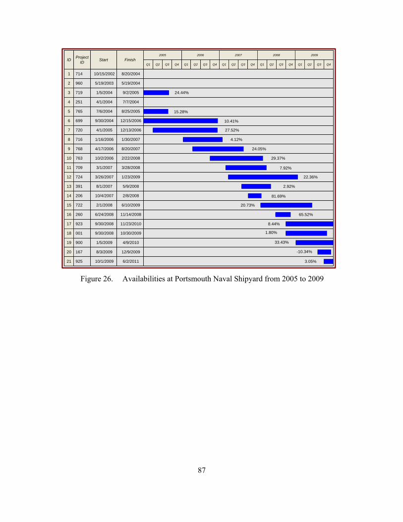
87

ID Project ID Start Finish

200720062005 20092008

Q2Q4Q3 Q1 Q2 Q3Q3Q2 Q4Q3 Q3Q2Q4 Q4 Q1Q1 Q1 Q4Q2Q1

1 8/20/200410/15/2002714

2 5/19/20045/19/2003960

3 9/2/20051/5/2004719

4 7/7/20044/1/2004251

5 8/25/20057/6/2004765

6 12/15/20069/30/2004699

7 12/13/20064/1/2005720

8 1/30/20071/16/2006716

9 8/20/20074/17/2006768

10 2/22/200810/2/2006763

11 3/28/20083/1/2007709

12 1/23/20093/26/2007724

13 5/9/20088/1/2007391

14 2/8/200810/4/2007206

15 6/10/20092/1/2008722

16 11/14/20086/24/2008260

17 11/23/20109/30/2008923

18 10/30/20099/30/2008001

19 4/9/20101/5/2009900

20 12/9/20098/3/2009167

21 6/2/201110/1/2009925

29.37%

24.05%

4.12%

27.52%

10.41%

15.28%

24.44%

8.44%

65.52%

20.73%

81.69%

2.92%

22.36%

7.92%

3.05%

-10.34%

33.43%

1.80%

Figure 26. Availabilities at Portsmouth Naval Shipyard from 2005 to 2009

88

ID ProjectID Start Finish

2009

Q1

1 7/8/200410/1/2001N13

2 12/23/200511/15/2002N26

3 7/30/20042/17/2003S59

6 12/6/20063/15/2004N27

7 12/15/200611/17/2004N62

2008

Q1 Q1Q2 Q3Q2Q1Q4 Q4Q3Q2Q3Q1

2006 2007

9 5/16/20081/18/2006S31

Q4Q2 Q3

10

12

5/26/20062/13/2006Q25

11/20/20068/1/2006Q54

15 4/14/200912/5/2006Q11

14 11/28/200811/1/2006RB2

26

22

20

19

16 9/11/20076/1/2007Q58

5/7/20102/7/200833Q

7/3/20083/5/200823A

12/19/20089/1/2008Q59

12/23/20102/12/201023B

4 6/7/20046/23/2003D72

8 12/20/20051/17/2005G74

5 8/23/20042/23/2004A68

11 9/1/20063/1/2006D68

13 6/29/20079/5/2006G72

18 3/27/20089/28/200774A

17 10/30/20075/1/2007A76

21 12/16/20086/16/200868B

24 1/15/20105/18/200972A

27 12/16/20106/14/201074B

23 5/7/20091/5/2009A73

25 5/11/20101/11/201073B

29 10/13/20116/15/2011MNA

2005

Q2Q3 Q4Q4

3.47%

0%

-.13%

0%

3.41%

73.33%

0%

3.74%

56.02%

0%

18.43%

12.09%

-0.55%

-0.55%

0%

0%

0%

0%

0%

0%

28 6/3/20111/10/201173C

Figure 27. Availabilities at Puget Sound Naval Shipyard from 2005 to 2009

89

APPENDIX B: AQWP AND BQWP STATISTICAL COMPARISON RESULTS

Two-sample t-tests, assuming unequal variances, are conducted to compare the

budgeted quantity of work planned (BQWP) per month (based on the planned duration)

against the actual quantity of work planned (AQWP) per month (based in terms of both

planned duration and actual duration).

A. AQWP AND BQWP PER MONTH FOR LATE AVAILABILITIES

Late Carriers BQWP/Month (planned) AQWP/Month (actual) Mean 28675.38333 27588.05481Variance 27602210.7 23688811.86Observations 8 8Hypothesized Mean Difference 0 df 14 t Stat -0.429422794 P(T<=t) one-tail 0.337075382 t Critical one-tail 1.761310115 P(T<=t) two-tail 0.674150765 t Critical two-tail 2.144786681

Late Submarines BQWP/Month (planned) AQWP/Month (actual) Mean 11826.04595 11076.599Variance 9037435.358 9475660.855Observations 56 56Hypothesized Mean Difference 0 df 110 t Stat -1.303453007 P(T<=t) one-tail 0.097570845 t Critical one-tail 1.658824188 P(T<=t) two-tail 0.19514169 t Critical two-tail 1.981765221

Table 36. T-test Results Comparing Means of AQWP/Month (Actual Duration) and BQWP/Month (Planned Duration) for Late Availabilities

90

Late Carriers BQWP/Month (planned) AQWP/Month (planned) Mean 28675.38333 31702.51989Variance 27602210.7 49647229.9Observations 8 8Hypothesized Mean Difference 0 df 13 t Stat -0.974157853 P(T<=t) one-tail 0.173878592 t Critical one-tail 1.770933383 P(T<=t) two-tail 0.347757183 t Critical two-tail 2.160368652

Late Submarines BQWP/Month (planned) AQWP/Month (planned) Mean 11826.04595 14045.87422Variance 9037435.358 16092768.44Observations 56 56Hypothesized Mean Difference 0 df 102 t Stat -3.313716773 P(T<=t) one-tail 0.000637503 t Critical one-tail 1.659929976 P(T<=t) two-tail 0.001275006 t Critical two-tail 1.983495205

Table 37. T-test Results Comparing Means of AQWP/Month (Planned Duration) and BQWP/Month (Planned Duration) for Late Availabilities

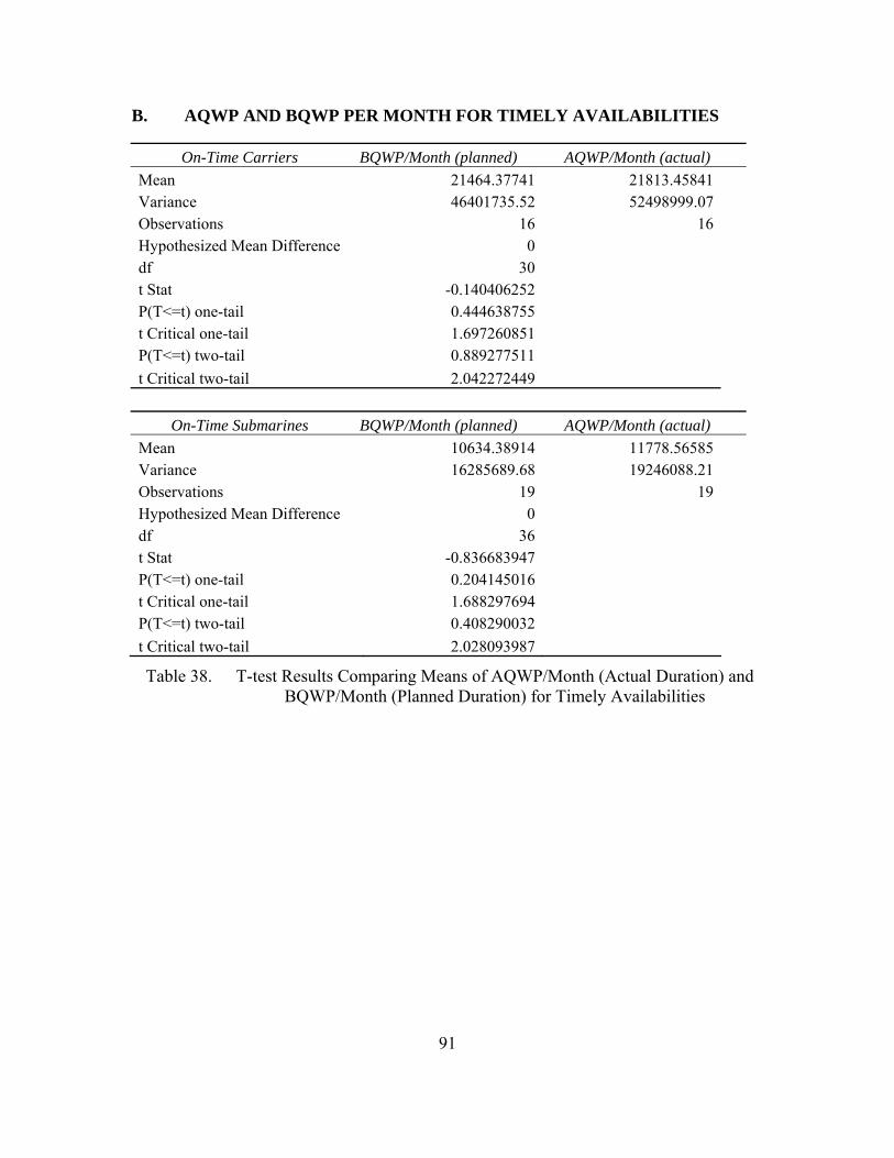
91

B. AQWP AND BQWP PER MONTH FOR TIMELY AVAILABILITIES

On-Time Carriers BQWP/Month (planned) AQWP/Month (actual) Mean 21464.37741 21813.45841 Variance 46401735.52 52498999.07 Observations 16 16 Hypothesized Mean Difference 0 df 30 t Stat -0.140406252 P(T<=t) one-tail 0.444638755 t Critical one-tail 1.697260851 P(T<=t) two-tail 0.889277511 t Critical two-tail 2.042272449

On-Time Submarines BQWP/Month (planned) AQWP/Month (actual) Mean 10634.38914 11778.56585 Variance 16285689.68 19246088.21 Observations 19 19 Hypothesized Mean Difference 0 df 36 t Stat -0.836683947 P(T<=t) one-tail 0.204145016 t Critical one-tail 1.688297694 P(T<=t) two-tail 0.408290032 t Critical two-tail 2.028093987

Table 38. T-test Results Comparing Means of AQWP/Month (Actual Duration) and BQWP/Month (Planned Duration) for Timely Availabilities

92

On-Time Carriers BQWP/Month (planned) AQWP/Month (planned) Mean 21464.37741 21727.44338 Variance 46401735.52 51890943.57 Observations 16 16 Hypothesized Mean Difference 0 df 30 t Stat -0.106136335 P(T<=t) one-tail 0.458090364 t Critical one-tail 1.697260851 P(T<=t) two-tail 0.916180728 t Critical two-tail 2.042272449

On-Time Submarines BQWP/Month (planned) AQWP/Month (planned) Mean 10634.38914 11493.5883 Variance 16285689.68 19202764.84 Observations 19 19 Hypothesized Mean Difference 0 df 36 t Stat -0.628676321 P(T<=t) one-tail 0.266764923 t Critical one-tail 1.688297694 P(T<=t) two-tail 0.533529847 t Critical two-tail 2.028093987

Table 39. T-test Results Comparing Means of AQWP/Month (Planned Duration) and BQWP/Month (Planned Duration) for Timely Availabilities

93

C. STANDARD ERRORS FOR MEAN AQWP AND BQWP PER MONTH

Mean AQWP/Month (Actual Duration)

Standard Error

Mean BQWP/Month (Planned Duration)

Standard Error

Late Sub Avails 11076.6 411.4 11826.1 401.7 On-Time Sub Avails 11778.6 1006.5 10634.4 925.8

Late Carrier Avails 27588.1 1720.8 28675.4 1857.5 On-Time Carriers 21813.46 1811.4 21464.4 1703.0

Late Sub DSRA 9532.9 539.1 11645.7 679.2 On-Time Sub DSRA 10848.7 641.8 9981.5 526.9

Late Sub ERO 15490.3 1592.8 14579.7 1370.0 On-Time Sub ERO 15216.4 330.6 14309.1 650.4

Late Sub DMP 12913.1 457.4 13332.1 567.0 On-Time Sub DMP 13508 1278.8 11280.1 1091.7

Late Sub IA 4870.1 191.3 4859.2 225.1 On-Time Sub IA 5102.2 418 4571.2 318.6 Late Carrier PIA 27889.7 1838.9 29932.2 2806.8

On-Time Carrier PIA 23211.3 1552.1 23146.8 1585.3

Mean AQWP/Month (Planned Duration)

Standard Error

Mean BQWP/Month (Planned Duration)

Standard Error

Late Sub Avails 14045.9 536.1 11826.1 401.7 On-Time Sub Avails 11493.6 1005.3 10634.4 925.8

Late Carrier Avails 31702.5 2491.2 28675.4 1857.5 On-Time Carriers 21727.4 1800.9 21464.4 1703.0

Table 40. Standard Errors for Mean AQWP per Month and Mean BQWP per Month in Man-Days

94


95

APPENDIX C: WORK STOPPAGE DATA BY LENGTH

The tables are organized with the columns representing the eight reasons for work

stoppage and the rows are the estimated number of work stoppages for each duration

measured in weeks; the durations are in units of weeks. The table is populated with the

number of work stoppages observed with respect to work stoppage reason and the

number of consecutive entries (labeled as duration).

A. COMPLETE WORK STOPPAGE DATA SETS

MAT IC TD TL SAF W WC RSC Total WS1 379 423 479 16 61 33 55 94 15402 142 186 150 0 1 9 22 36 5463 49 86 77 0 2 3 20 15 2524 36 53 35 0 1 4 6 8 1435 19 26 8 0 0 0 2 1 566 21 14 14 0 3 3 1 3 597 12 11 5 0 1 0 2 3 348 2 4 5 0 0 0 1 0 129 5 5 6 0 1 0 0 1 18

10 3 3 0 0 0 0 1 0 711 0 2 3 0 0 0 2 0 712 0 1 0 0 0 1 0 0 213 0 0 0 0 0 0 1 0 114 0 1 0 0 0 0 0 0 115 1 0 0 0 0 0 0 0 116 1 1 0 0 0 0 0 0 217 0 0 0 0 0 0 0 0 018 0 0 0 0 0 0 0 0 019 0 0 0 0 0 0 0 0 020 0 0 0 0 0 0 0 0 0

Total 670 816 782 16 70 53 113 161 2681

2.06 2.12 1.84 1.00 1.53 2.00 2.35 1.84 1.99

1.83 1.79 1.52 0.00 1.57 1.94 2.21 1.40 1.730.07 0.06 0.05 0.00 0.19 0.27 0.21 0.11 0.03

Dur

atio

n (w

eeks

)


Mean Length of Stoppage (weeks)Standard Deviation

Standard Error of Mean Table 41. EISENHOWER (CVN 69) PIA

96


10 0 0 0 0 0 0 0 0 011 0 0 0 0 0 0 0 0 012 0 0 0 0 0 0 0 0 013 0 0 0 0 0 0 0 0 014 0 0 0 0 0 0 0 0 015 0 0 0 0 0 0 0 0 016 0 0 0 0 0 0 0 0 017 0 0 0 0 0 0 0 0 018 0 0 0 0 0 0 0 0 019 0 0 0 0 0 0 0 0 020 0 0 0 0 0 0 0 0 0

Total 119 21 120 2 1 10 14 6 293

1.83 1.24 1.50 2.50 1.00 2.20 1.57 1.33 1.65

1.31 0.53 0.99 1.50 0.00 1.72 0.90 0.47 1.160.12 0.11 0.09 1.06 0.00 0.54 0.24 0.19 0.07Standard Error of Mean


Dur

atio

n (w

eeks

)


Table 42. GEORGE WASHINGTON (CVN 73) SRA


10 0 0 0 0 0 0 1 0 111 0 0 0 0 0 0 0 0 012 0 0 0 0 0 0 0 0 013 0 0 0 0 0 0 0 0 014 0 0 0 0 0 0 0 0 015 0 0 0 0 0 0 0 0 016 0 0 0 0 0 0 0 0 017 0 0 0 0 0 0 0 0 018 0 0 0 0 0 0 0 0 019 0 0 0 0 0 0 0 0 020 0 0 0 0 0 0 0 0 0

Total 119 173 213 18 0 2 30 24 579

1.40 1.86 1.41 1.39 0.00 1.50 1.77 1.29 1.56

0.69 1.29 0.83 0.59 0.00 0.50 1.76 0.61 1.040.06 0.10 0.06 0.14 0.00 0.35 0.32 0.12 0.04


Dur

atio

n (w

eeks

)


Standard Error of Mean Table 43. COLUMBUS (SSN 762) DSRA

97


10 0 0 0 0 0 0 0 0 011 0 0 0 0 0 0 0 0 012 0 0 0 0 0 0 0 0 013 0 0 0 0 0 0 0 0 014 0 0 0 0 0 0 0 0 015 0 0 0 0 0 0 0 0 016 0 0 0 0 0 0 0 0 017 0 0 0 0 0 0 0 0 018 0 0 0 0 0 0 0 0 019 0 0 0 0 0 0 0 0 020 0 0 0 0 0 0 0 0 0

Total 101 149 30 1 2 0 6 5 294

1.61 1.70 1.60 2.00 2.00 0.00 1.50 1.60 1.66

1.08 1.16 0.80 0.00 1.00 0.00 0.76 1.20 1.090.11 0.10 0.15 0.00 0.71 0.00 0.31 0.54 0.06


Standard Error of Mean


Dur

atio

n (w

eeks

)

Table 44. MICHIGAN (SSGN 727) MMP


10 0 4 0 0 0 0 1 0 511 0 0 0 0 0 0 0 0 012 0 1 0 0 0 0 0 0 113 0 0 0 0 0 1 0 0 114 0 0 0 0 0 0 0 0 015 0 0 0 0 0 0 0 0 016 0 0 0 0 0 0 0 0 017 0 0 0 0 0 0 0 0 018 0 0 0 0 0 0 0 0 019 0 0 0 0 0 0 0 0 020 0 0 0 0 0 0 0 0 0

Total 334 535 310 14 5 15 44 138 1395

1.88 2.18 1.76 1.36 2.00 3.00 2.20 1.67 1.97

1.21 1.71 1.30 1.04 2.00 3.27 2.22 1.08 1.520.07 0.07 0.07 0.28 0.89 0.84 0.33 0.09 0.04

Dur

atio

n (w

eeks

)




Table 45. JOHN C STENNIS (CVN 74) PIA

98


10 0 0 0 0 0 0 0 0 011 0 0 0 0 0 0 0 0 012 0 0 0 0 0 0 0 0 013 0 0 0 0 0 0 0 0 014 0 0 0 0 0 0 0 0 015 0 0 0 0 0 0 0 0 016 0 0 0 0 0 0 0 0 017 0 0 0 0 0 0 0 0 018 0 0 0 0 0 0 0 0 019 0 0 0 0 0 0 0 0 020 0 0 0 0 0 0 0 0 0

Total 32 50 25 0 0 6 2 2 117

1.09 1.34 1.24 0.00 0.00 1.50 1.50 1.00 1.26

0.29 0.76 0.86 0.00 0.00 1.12 0.50 0.00 0.720.05 0.11 0.17 0.00 0.00 0.46 0.35 0.00 0.07

Dur

atio

n (w

eeks

)




Table 46. NORFOLK (SSN 714) CM

99

B. RED COLOR-CODED WORK STOPPAGE DATA SETS


10 0 0 0 0 0 0 0 0 011 0 0 0 0 0 0 0 0 012 0 1 0 0 0 0 0 0 113 0 0 0 0 0 0 0 0 014 0 0 0 0 0 0 0 0 015 0 0 0 0 0 0 0 0 016 0 0 0 0 0 0 0 0 017 0 0 0 0 0 0 0 0 018 0 0 0 0 0 0 0 0 019 0 0 0 0 0 0 0 0 020 0 0 0 0 0 0 0 0 0

Total 177 217 158 2 9 9 35 34 641

1.34 1.55 1.34 1.00 1.00 1.00 1.37 1.29 1.40



Dur

atio

n (w

eeks

)


Table 47. EISENHOWER (CVN 69) PIA


10 0 0 0 0 0 0 0 0 011 0 0 0 0 0 0 0 0 012 0 0 0 0 0 0 0 0 013 0 0 0 0 0 0 0 0 014 0 0 0 0 0 0 0 0 015 0 0 0 0 0 0 0 0 016 0 0 0 0 0 0 0 0 017 0 0 0 0 0 0 0 0 018 0 0 0 0 0 0 0 0 019 0 0 0 0 0 0 0 0 020 0 0 0 0 0 0 0 0 0

Total 33 10 31 0 1 3 7 3 88

1.39 1.30 1.19 0.00 1.00 1.33 1.43 1.33 1.31



Dur

atio

n (w

eeks

)



100


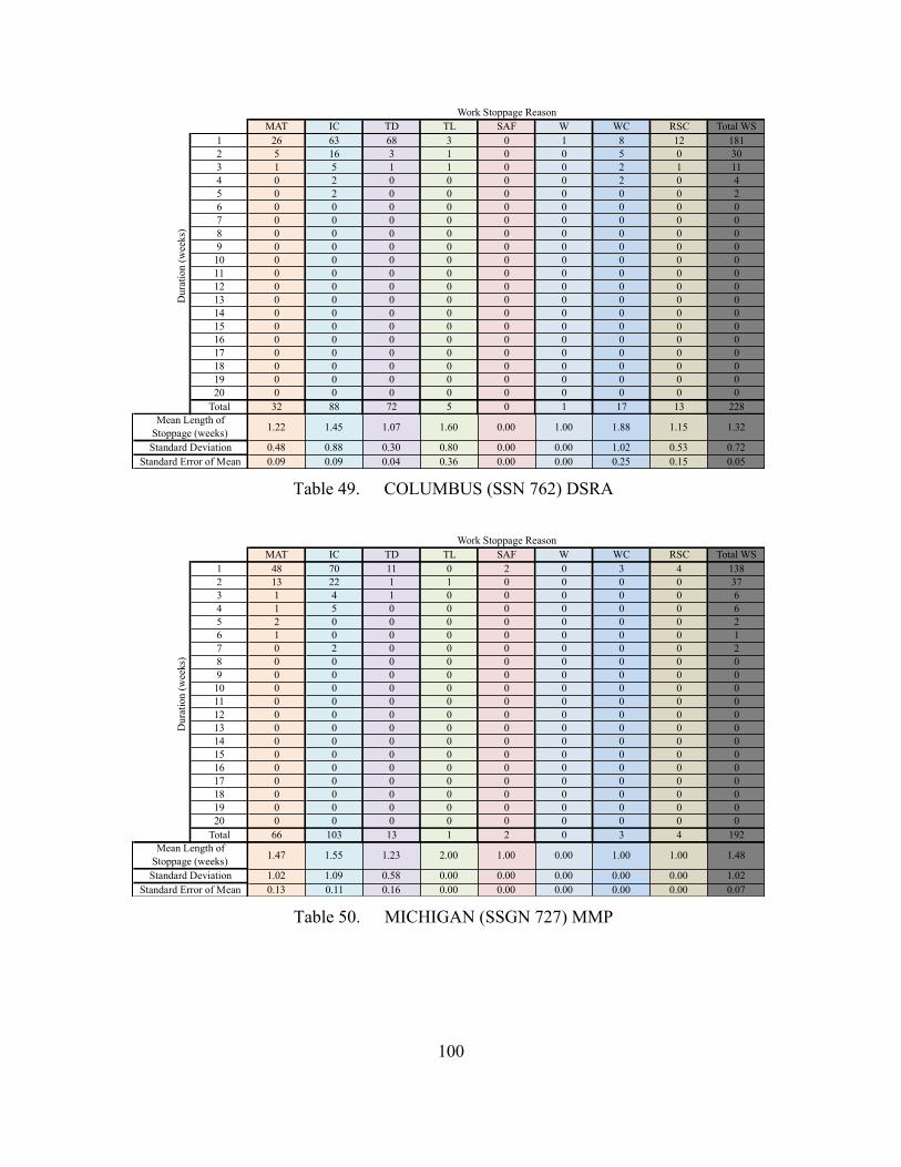
10 0 0 0 0 0 0 0 0 011 0 0 0 0 0 0 0 0 012 0 0 0 0 0 0 0 0 013 0 0 0 0 0 0 0 0 014 0 0 0 0 0 0 0 0 015 0 0 0 0 0 0 0 0 016 0 0 0 0 0 0 0 0 017 0 0 0 0 0 0 0 0 018 0 0 0 0 0 0 0 0 019 0 0 0 0 0 0 0 0 020 0 0 0 0 0 0 0 0 0

Total 32 88 72 5 0 1 17 13 228

1.22 1.45 1.07 1.60 0.00 1.00 1.88 1.15 1.32



Dur

atio

n (w

eeks

)


Table 49. COLUMBUS (SSN 762) DSRA


10 0 0 0 0 0 0 0 0 011 0 0 0 0 0 0 0 0 012 0 0 0 0 0 0 0 0 013 0 0 0 0 0 0 0 0 014 0 0 0 0 0 0 0 0 015 0 0 0 0 0 0 0 0 016 0 0 0 0 0 0 0 0 017 0 0 0 0 0 0 0 0 018 0 0 0 0 0 0 0 0 019 0 0 0 0 0 0 0 0 020 0 0 0 0 0 0 0 0 0

Total 66 103 13 1 2 0 3 4 192

1.47 1.55 1.23 2.00 1.00 0.00 1.00 1.00 1.48



Dur

atio

n (w

eeks

)



101


10 0 0 0 0 0 0 0 0 011 0 0 0 0 0 0 0 0 012 0 0 0 0 0 0 0 0 013 0 0 0 0 0 0 0 0 014 0 0 0 0 0 0 0 0 015 0 0 0 0 0 0 0 0 016 0 0 0 0 0 0 0 0 017 0 0 0 0 0 0 0 0 018 0 0 0 0 0 0 0 0 019 0 0 0 0 0 0 0 0 020 0 0 0 0 0 0 0 0 0

Total 50 111 38 2 0 4 14 7 226

1.22 1.59 1.21 1.00 0.00 1.25 1.57 1.43 1.42



Dur

atio

n (w

eeks

)




10 0 0 0 0 0 0 0 0 011 0 0 0 0 0 0 0 0 012 0 0 0 0 0 0 0 0 013 0 0 0 0 0 0 0 0 014 0 0 0 0 0 0 0 0 015 0 0 0 0 0 0 0 0 016 0 0 0 0 0 0 0 0 017 0 0 0 0 0 0 0 0 018 0 0 0 0 0 0 0 0 019 0 0 0 0 0 0 0 0 020 0 0 0 0 0 0 0 0 0

Total 13 30 14 0 0 3 2 2 64

1.00 1.30 1.14 0.00 0.00 1.33 1.00 1.00 1.19



Dur

atio

n (w

eeks

)



102


103

APPENDIX D: WORK STOPPAGE DATA BY QUANTITY

The work stoppage entries are counted and sorted into the appropriate reason

categories.


MAT IC TD TL SAF W WC RSC WS Total


670 816 782 16 70 53 113 161 2681


119 21 120 2 1 10 14 6 293


119 173 213 18 0 2 30 24 579


101 149 30 1 2 0 6 5 294


334 535 310 14 5 15 44 138 1395


32 50 25 0 0 6 2 2 117

Num

ber o

f Wor

k St

oppa

ges


Table 53. Quantity of Work Stoppages


MAT IC TD TL SAF W WC RSC WS Total


177 217 158 2 9 9 35 34 641


33 10 31 0 1 3 7 3 88


32 88 72 5 0 1 17 13 228


66 103 13 1 2 0 3 4 192


50 111 38 2 0 4 14 7 226


13 30 14 0 0 3 2 2 64


Num

ber o

f Wor

k St

oppa

ges

Table 54. Quantity of Red Color-Coded Work Stoppages

104


105

APPENDIX E: WORK STOPPAGES BY TIME-IN-AVAILABILITY

The work stoppages are sorted based on reason and by time during the availability in

which experienced. The figures corresponding to each table display the number of

material (MAT), interference/coordination (IC), and technical direction (TD) work

stoppages against the time-in-availability.


MAT IC TD TL SAF W WC RSC Total WSPrior to SA00 123 21 197 0 0 0 4 1 346

0%-10% 30 73 56 1 2 2 2 12 17810%-20% 45 29 77 1 1 0 8 5 16620%-30% 61 79 72 2 0 5 3 19 24130%-40% 50 62 83 1 52 1 15 34 29840%-50% 41 84 70 0 2 2 7 29 23550%-60% 36 121 50 8 0 10 10 19 25460%-70% 104 139 90 2 0 7 24 25 39170%-80% 52 78 31 0 3 1 7 10 18280%-90% 62 81 40 0 1 4 14 5 207

90%-100% 15 18 4 1 1 9 4 1 53Post-Planned CA00 51 31 12 0 8 12 15 1 130

Perc

enta

ge o

f Pla

nned

Dur

atio

n



0

50

100

150

200

250

Prior to

SA00

0%-10

%

10%-20

%

20%-30

%

30%-40

%

40%-50

%

50%-60

%

60%-70

%

70%-80

%

80%-90

%

90%-10

0%

Post-Plan

ned C

A00

Num

ber

of W

ork

Stop

page

s

MAT

IC

TD

Figure 28. EISENHOWER (CVN 69) PIA

106

MAT IC TD TL SAF W WC RSC TotalPrior to SA00 11 3 13 0 0 0 0 1 28

0%-10% 9 2 5 0 0 0 1 1 1810%-20% 11 2 12 0 0 0 0 1 2620%-30% 20 10 28 1 1 3 2 1 6630%-40% 14 0 17 0 0 0 0 1 3240%-50% 21 3 14 1 0 2 3 1 4550%-60% 14 0 12 0 0 3 2 0 3160%-70% 1 0 0 0 0 0 0 0 170%-80% 8 0 5 0 0 2 0 0 1580%-90% 1 0 2 0 0 0 1 0 4

90%-100% 1 0 5 0 0 0 2 0 8Post-Planned CA00 8 1 7 0 0 0 3 0 19


Perc

enta

ge o

f Pla

nned

Dur

atio

n


0

5

10

15

20

25

30

Prior to

SA00

0%-10

%

10%-20

%

20%-30

%

30%-40

%

40%-50

%

50%-60

%

60%-70

%

70%-80

%

80%-90

%

90%-10

0%

Post-Plan

ned C

A00

Num

ber

of W

ork

Stop

page

s

MAT

IC

TD

Figure 29. GEORGE WASHINGTON (CVN 73) SRA

107


0%-10% 41 23 32 7 0 1 6 4 11410%-20% 26 7 29 1 0 0 0 0 6320%-30% 17 51 49 3 0 1 4 3 12830%-40% 1 11 20 1 0 0 0 4 3740%-50% 7 24 16 3 0 0 4 3 5750%-60% 1 5 7 0 0 0 0 0 1360%-70% 5 18 20 0 0 0 2 5 5070%-80% 1 4 3 0 0 0 0 1 980%-90% 3 4 6 0 0 0 2 0 15

90%-100% 0 17 7 0 0 0 1 1 26Post-Planned CA00 2 5 8 0 0 0 0 1 16


Perc

enta

ge o

f Pla

nned

Dur

atio

n


0

10

20

30

40

50

60

Prior to

SA00

0%-10

%

10%-20

%

20%-30

%

30%-40

%

40%-50

%

50%-60

%

60%-70

%

70%-80

%

80%-90

%

90%-10

0%

Post-Plan

ned C

A00

Num

ber

of W

ork

Stop

page

s

MAT

IC

TD

Figure 30. COLUMBUS (SSN 762) DSRA

108


0%-10% 1 0 0 0 0 0 0 0 110%-20% 15 7 3 0 0 0 2 1 2820%-30% 1 6 4 0 0 0 0 0 1130%-40% 12 34 8 0 1 0 2 1 5840%-50% 21 20 5 1 0 0 1 1 4950%-60% 16 26 3 0 0 0 0 2 4760%-70% 7 24 1 0 1 0 1 0 3470%-80% 15 10 2 0 0 0 0 0 2780%-90% 1 2 0 0 0 0 0 0 3

90%-100% 1 12 0 0 0 0 0 0 13Post-Planned CA00 1 6 0 0 0 0 0 0 7


Perc

enta

ge o

f Pla

nned

Dur

atio

n


0 5

10 15 20 25 30 35 40

Prior to

SA00

0%-10

%

10%-20

%

20%-30

%

30%-40

%

40%-50

%

50%-60

%

60%-70

%

70%-80

%

80%-90

%

90%-10

0%

Post-Plan

ned C

A00

Num

ber

of W

ork

Stop

page

s

MAT

IC

TD

Figure 31. MICHIGAN (SSGN 727) MMP

109


0%-10% 13 19 27 0 0 0 10 8 7710%-20% 32 48 40 2 1 0 1 16 14020%-30% 21 62 38 1 1 2 1 20 14630%-40% 47 62 54 4 2 1 3 26 19940%-50% 61 126 51 2 1 5 9 19 27450%-60% 57 108 61 2 0 6 5 30 26960%-70% 52 89 21 3 0 0 4 10 17970%-80% 38 10 2 0 0 0 2 2 5480%-90% 7 10 4 0 0 0 1 0 22

90%-100% 1 1 0 0 0 0 1 0 3Post-Planned CA00 1 0 0 0 0 0 0 0 1


Perc

enta

ge o

f Pla

nned

Dur

atio

n


0

20

40

60

80

100

120

140

Prior to

SA00

0%-10

%

10%-20

%

20%-30

%

30%-40

%

40%-50

%

50%-60

%

60%-70

%

70%-80

%

80%-90

%

90%-10

0%

Post-Plan

ned C

A00

Num

ber

of W

ork

Stop

page

s

MAT

IC

TD

Figure 32. JOHN C STENNIS (CVN 74) PIA


0%-10% 0 0 0 0 0 0 0 0 010%-20% 0 0 0 0 0 0 0 0 020%-30% 0 0 0 0 0 0 0 0 030%-40% 9 12 9 0 0 1 0 0 3140%-50% 5 13 7 0 0 2 0 0 2750%-60% 11 8 3 0 0 1 1 0 2460%-70% 3 9 3 0 0 0 0 0 1570%-80% 0 5 1 0 0 0 1 1 880%-90% 4 3 2 0 0 2 0 1 12

90%-100% 0 0 0 0 0 0 0 0 0Post-Planned CA00 0 0 0 0 0 0 0 0 0


Perc

enta

ge o

f Pla

nned

Dur

atio

n

110


0

2

4

6

8

10

12

14

Prior to

SA00

0%-10

%

10%-20

%

20%-30

%

30%-40

%

40%-50

%

50%-60

%

60%-70

%

70%-80

%

80%-90

%

90%-10

0%

Post-Plan

ned C

A00

Num

ber

of W

ork

Stop

page

s

MAT

IC

TD

Figure 33. NORFOLK (SSN 714) CM

EISENHOWER PIA






10% 66.03% 60.66% 30.86% 93.80% 28.68% 0.00%20% 50.14% 38.76% 22.33% 35.44% 12.49% 0.00%30% 37.16% 20.22% 14.30% 28.47% 7.86% 0.00%40% 28.15% 16.41% 12.95% 13.99% 5.22% 0.00%50% 23.63% 12.98% 11.31% 9.78% 3.57% 0.00%60% 20.14% 11.34% 11.00% 7.59% 2.73% 0.00%70% 16.41% 11.30% 9.92% 6.54% 2.36% 0.00%80% 15.10% 10.65% 9.75% 5.88% 2.26% 0.00%90% 13.85% 10.49% 9.48% 5.82% 2.23% 0.00%100% 13.56% 10.18% 9.04% 5.56% 2.22% 0.00%

Post-Planned CA00 12.91% 9.52% 8.79% 5.42% 2.22% 0.00%

Poin

t in

Tim

e of

Ava

ilabi

lity

Table 61. Pre-availability Work Stoppage Ratio

111



0%-10% 5 4 2 0 0 1 0 1 1310%-20% 7 3 9 0 0 0 0 0 1920%-30% 10 8 4 0 0 0 1 2 2530%-40% 7 23 13 0 9 0 1 6 5940%-50% 6 20 4 0 0 0 1 6 3750%-60% 9 20 30 2 0 1 1 9 7260%-70% 22 55 15 0 0 0 2 2 9670%-80% 24 29 18 0 0 0 2 5 7880%-90% 31 25 16 0 0 2 9 3 86

90%-100% 2 6 1 0 0 1 3 0 13Post-Planned CA00 30 16 10 0 0 4 15 0 75

Work Stoppage ReasonPe

rcen

tage

of P

lann

ed D

urat

ion


0

10

20

30

40

50

60

Prior to

SA00

0%-10

%

10%-20

%

20%-30

%

30%-40

%

40%-50

%

50%-60

%

60%-70

%

70%-80

%

80%-90

%

90%-10

0%

Post-Plan

ned C

A00

Num

ber

of W

ork

Stop

page

s

MAT

IC

TD

Figure 34. EISENHOWER (CVN 69) PIA

112


0%-10% 1 0 1 0 0 0 0 0 210%-20% 0 1 4 0 0 0 0 0 520%-30% 5 5 4 0 1 3 1 1 2030%-40% 3 0 2 0 0 0 0 1 640%-50% 5 1 4 0 0 0 2 0 1250%-60% 7 0 9 0 0 0 1 0 1760%-70% 0 0 0 0 0 0 0 0 070%-80% 1 0 0 0 0 0 0 0 180%-90% 0 0 0 0 0 0 0 0 0

90%-100% 0 0 0 0 0 0 0 0 0Post-Planned CA00 6 0 3 0 0 0 3 0 12


Perc

enta

ge o

f Pla

nned

Dur

atio

n


0 1 2 3 4 5 6 7 8 9

10

Prior to

SA00

0%-10

%

10%-20

%

20%-30

%

30%-40

%

40%-50

%

50%-60

%

60%-70

%

70%-80

%

80%-90

%

90%-10

0%

Post-Plan

ned C

A00

Num

ber

of W

ork

Stop

page

s

MAT

IC

TD

Figure 35. GEORGE WASHINGTON (CVN 73) SRA

113


0%-10% 6 6 5 1 0 0 2 2 2210%-20% 4 4 4 0 0 0 0 0 1220%-30% 8 15 18 0 0 1 3 1 4630%-40% 0 4 5 1 0 0 0 1 1140%-50% 4 13 6 3 0 0 4 2 3250%-60% 2 4 1 0 0 0 0 0 760%-70% 1 11 12 0 0 0 3 5 3270%-80% 0 4 0 0 0 0 0 0 480%-90% 1 2 2 0 0 0 1 0 6

90%-100% 0 18 7 0 0 0 1 1 27Post-Planned CA00 2 5 8 0 0 0 0 1 16


Perc

enta

ge o

f Pla

nned

Dur

atio

n


0 2 4 6 8

10 12 14 16 18 20

Prior to

SA00

0%-10

%

10%-20

%

20%-30

%

30%-40

%

40%-50

%

50%-60

%

60%-70

%

70%-80

%

80%-90

%

90%-10

0%

Post-Plan

ned C

A00

Num

ber

of W

ork

Stop

page

s

MAT

IC

TD

Figure 36. COLUMBUS (SSN 762) DSRA

114


0%-10% 0 0 0 0 0 0 0 0 010%-20% 5 4 2 0 0 0 1 1 1320%-30% 1 3 1 0 0 0 0 0 530%-40% 4 20 1 0 0 0 0 1 2640%-50% 18 10 3 1 0 0 1 0 3350%-60% 14 30 3 0 1 0 0 2 5060%-70% 6 11 1 0 1 0 1 0 2070%-80% 10 4 1 0 0 0 0 0 1580%-90% 0 1 0 0 0 0 0 0 1

90%-100% 1 13 0 0 0 0 0 0 14Post-Planned CA00 1 6 0 0 0 0 0 0 7


Perc

enta

ge o

f Pla

nned

Dur

atio

n


0

5

10

15

20

25

30

35

Prior to

SA00

0%-10

%

10%-20

%

20%-30

%

30%-40

%

40%-50

%

50%-60

%

60%-70

%

70%-80

%

80%-90

%

90%-10

0%

Post-Plan

ned C

A00

Num

ber

of W

ork

Stop

page

s

MAT

IC

TD

Figure 37. MICHIGAN (SSGN 727) MMP

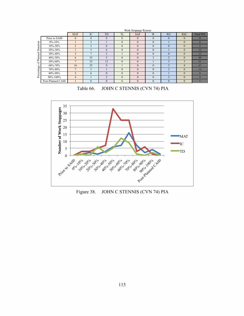
115


0%-10% 1 3 1 0 0 0 1 0 610%-20% 2 3 0 0 0 0 0 0 520%-30% 1 5 6 0 0 0 1 0 1330%-40% 3 7 2 1 0 0 0 0 1340%-50% 6 33 5 0 0 3 2 0 4950%-60% 7 25 12 0 0 1 3 3 5160%-70% 16 25 9 1 0 0 2 4 5770%-80% 7 3 1 0 0 0 2 0 1380%-90% 2 6 0 0 0 0 1 0 9

90%-100% 4 1 2 0 0 0 2 0 9Post-Planned CA00 1 0 0 0 0 0 0 0 1


Perc

enta

ge o

f Pla

nned

Dur

atio

n


0

5

10

15

20

25

30

35

Prior to

SA00

0%-10

%

10%-20

%

20%-30

%

30%-40

%

40%-50

%

50%-60

%

60%-70

%

70%-80

%

80%-90

%

90%-10

0%

Post-Plan

ned C

A00

Num

ber

of W

ork

Stop

page

s

MAT

IC

TD

Figure 38. JOHN C STENNIS (CVN 74) PIA

116


0%-10% 0 0 0 0 0 0 0 0 010%-20% 0 0 0 0 0 0 0 0 020%-30% 0 0 0 0 0 0 0 0 030%-40% 3 5 5 0 0 0 0 0 1340%-50% 0 6 3 0 0 0 0 0 950%-60% 6 6 1 0 0 1 1 0 1560%-70% 1 8 3 0 0 0 0 0 1270%-80% 0 3 0 0 0 0 1 1 580%-90% 3 2 2 0 0 2 0 1 10

90%-100% 0 0 0 0 0 0 0 0 0Post-Planned CA00 0 0 0 0 0 0 0 0 0

Perc

enta

ge o

f Pla

nned

Dur

atio

n



0 1 2 3 4 5 6 7 8 9

Prior to

SA00

0%-10

%

10%-20

%

20%-30

%

30%-40

%

40%-50

%

50%-60

%

60%-70

%

70%-80

%

80%-90

%

90%-10

0%

Post-Plan

ned C

A00

Num

ber

of W

ork

Stop

page

s

MAT

IC

TD

Figure 39. NORFOLK (SSN 714) CM

EISENHOWER PIA






10% 83.95% 86.67% 37.14% 100.00% 0.00% 0.00%20% 68.00% 65.00% 27.66% 38.10% 0.00% 0.00%30% 54.40% 32.50% 13.98% 30.77% 0.00% 0.00%40% 36.96% 28.26% 12.50% 15.38% 0.00% 0.00%50% 30.77% 22.41% 9.56% 9.41% 0.00% 0.00%60% 23.21% 17.33% 9.09% 5.93% 0.00% 0.00%70% 17.48% 17.33% 7.43% 5.16% 0.00% 0.00%80% 14.56% 17.11% 7.26% 4.71% 0.00% 0.00%90% 12.30% 17.11% 7.03% 4.68% 0.00% 0.00%

100% 12.01% 17.11% 6.13% 4.32% 0.00% 0.00%Post-Planned CA00 10.61% 14.77% 5.70% 4.17% 0.00% 0.00%

Poin

t in

Tim

e of

Ava

ilabi

lity

Table 68. Pre-availability Work Stoppage Ratio

117

LIST OF REFERENCES

Blanchard, Benjamin S., and Wolter J. Fabyrke. 2011. Systems Engineering and Analysis. Upper Saddle River, NJ: Prentice Hall.

Hayter, A. 2007. Probability and Statistics for Engineers and Scientists, 3rd ed. Belmont, CA: Duxbury.

Kerzner, Harold. 2009. Project Management: A Systems Approach to Planning, Scheduling, and Controlling, 10th ed. Hoboken, NJ: John Wiley & Sons, Inc.

Langford, Gary. “Project Scheduling,” Naval Postgraduate School SI3400 Lecture, 18 January 2011.

McMullen, Thomas B. 1998. Introduction to the Theory of Constraints (TOC) Management System. Boca Raton, FL: CRC Press LLC.

Mueller, R. K. 1996. Anchoring Points for Corporate Directors: Obeying the Unenforcable. London: Quorum Books.

NAVSEA (Naval Sea Systems Command). 2009. Strategic Business Plan 2009–2013.

NAVSEA 04X (Assistant Deputy Commander Industrial Operations, Naval Shipyards). 2009. “Execution Priorities (ERP).” Chap. 6A in AIM-NG Process Manual.

NAVSEA 04X (Assistant Deputy Commander Industrial Operations, Naval Shipyards). 2011. Monthly Project Management Lean Release 2.0/3.0 Implementation Results, Report Date 04 October 2011, Powerpoint Slides.

NAVSEA 04Z (Director, SUPSHIP Management Group). 2011. SUPSHIP Organizational Manual. Chapter 1: Mission and Organization.

NAVSEA 07 (Deputy Commander for Undersea Warfare). 2009. Baseline Project Management Plan for SSN 688 and SSN 21 Class Depot Modernization Periods, Engineering Overhauls and SSBN 726 Class Engineered Refueling Overhauls Availability Improved Planning and Execution, Revision C, NAVSEAINST 4790.23 REV C.

NAVSEA 07 (Deputy Commander for Undersea Warfare). 2011. Naval Shipyard Performance for Depot Level Submarine Availabilities – Potential Thesis Topic.

OPNAV N43 (Director, Fleet Readiness). 2010. “Representative Intervals, Durations, and Repair Mandays for Depot Level Maintenance Availabilities of U.S. Navy Ships.” Enclosure 3 in OPNAVNOTE 4700.

OPNAV N431 (Fleet Readiness and Logistics). 2010. Maintenance Policy for United States Navy Ships, OPNAVINST 4700.7L.

118


119

INITIAL DISTRIBUTION LIST

1. Defense Technical Information Center Ft. Belvoir, Virginia 2. Dudley Knox Library Naval Postgraduate School Monterey, California 3. Rear Admiral David Duryea Deputy Commander via Mark Ferguson, PMS 392 Naval Sea Systems Command, Undersea Warfare (SEA 07) Washington Navy Yard, D.C. 4. Rear Admiral Winford Ellis (ret.) Director of the Undersea Warfare Research Center Wayne E. Meyer Institute of Systems Engineering Monterey, California 5. Captain William Greene Chief of Staff Naval Sea Systems Command, SEA 4A Washington Navy Yard, D.C. 6. James Arsenault Naval Sea Systems Command 04XO Availability Performance Branch Head Washington Navy Yard, D.C.