Embed Size (px)
Citation preview
Nature or Nurture?
Learning and the Geography of Female Labor
Force Participation
Alessandra Fogli∗
University of Minnesotaand CEPR
Laura VeldkampNYU Stern School of Business
and NBER
March 12, 2010
Abstract
One of the most dramatic economic transformations of the past century has been the entryof women into the labor force. While many theories explain why this change took place, we in-vestigate the process of transition itself. We argue that local information transmission generateschanges in participation that are geographically heterogeneous, locally correlated and smoothin the aggregate, just like those observed in our data. In our model, women learn about theeffects of maternal employment on children by observing nearby employed women. When fewwomen participate in the labor force, data is scarce and participation rises slowly. As informa-tion accumulates in some regions, the effects of maternal employment become less uncertain,and more women in that region participate. Learning accelerates, labor force participation risesfaster, and regional participation rates diverge. Eventually, information diffuses throughout theeconomy, beliefs converge to the truth, participation flattens out and regions become more sim-ilar again. To investigate the empirical relevance of our theory, we use a new county-level dataset to compare our calibrated model to the time-series and geographic patterns of participation.
∗Corresponding author: [email protected], 44 West Fourth St., suite 7-77, New York, NY 10012, tel:(212)998-0527. We thank seminar participants at Northwestern, the World Bank, Chicago GSB, Wisconsin Madison,Minneapolis Federal Reserve, Princeton, European University in Florence, University of Southern California, NewYork University, Boston University, Bocconi, Pompeu Fabra, Ente Einaudi, Boston Federal Reserve and HarvardUniversity and conference participants at the 2009 winter NBER EF&G meetings, 2008 AEA, SITE, the 2007 NBERSummer Institute, the SED conference, LAEF Households, Gender and Fertility conference, the NBER group onMacroeconomics across Time and Space, Midwest Macro Meetings, the NY/Philadelphia Workshop on QuantitativeMacro, IZA/SOLE and Ammersee. We especially thank Stefania Marcassa for excellent research assistance andStefania Albanesi, Roland Benabou, Raquel Bernal, Jason Faberman, Jeremy Greenwood, Luigi Guiso, Larry Jones,Patrick Kehoe, Narayana Kocherlakota, Ellen McGrattan, Fabrizio Perri, Harald Uhlig and our anonymous refereesfor comments and suggestions. Laura Veldkamp thanks Princeton University for their hospitality and financialsupport through the Kenen fellowship. Keywords: female labor force participation, information diffusion, economicgeography. JEL codes: E2, N32, R1, J16.

Over the twentieth century, there has been a dramatic rise in female labor force participation in
the United States. Many theories of this phenomenon have been proposed. Some of them emphasize
the role played by market prices and technological factors; others focus on the role played by policies
and institutions, and a few recent ones investigate the role of cultural factors. All of them, however,
focus on aggregate shocks that explain why the transition took place and abstract from the local
interactions that could explain how the transition took place.
We use new data and theory to argue that women’s labor force participation decisions rely
on information that is transmitted from one woman to another, located nearby. The local nature
of information transmission smooths the effects of changes in the environment and generates ge-
ographically heterogeneous, but locally correlated reactions, like those observed in our data. Our
theory focuses on learning and participation of married women with young children, because this
sub-group is responsible for most of the rise in participation. A crucial factor in mothers’ participa-
tion decisions is the effect of employment on their children. However, this effect is uncertain. The
uncertainty makes risk-averse women less likely to participate. Learning resolves their uncertainty,
causing participation to rise.
In our overlapping generations model, women learn from their neighbors about the relative
importance of nature (innate ability) and nurture (the role of maternal employment) in determin-
ing children’s outcomes (section 1). Women inherit their parents’ beliefs and update them after
observing the outcomes of neighboring women in the previous generation. Those outcomes reveal
information about the effect of maternal employment only if the neighboring mothers were em-
ployed. Section 2 shows that higher local participation generates more information, which reduces
uncertainty about the effect of maternal employment and makes participation of nearby women
more likely. Thus, local participation snowballs and a gradual, but geographically-concentrated
rise in participation rates ensues.
Using county-level U.S. data from 1940-2000, section 3 documents how the growth rate of
women’s labor force varied over time and across counties.1 After the shift from an agricultural to1To our knowledge this county-level Historical, Demographic, Economic and Social Data has not been explored
before in economics research.
1

industrial economy separated the location of home and work, the female labor force grew slowly up
through the post-war decades, accelerated during the 1970s and 1980s, and recently flattened out.
Furthermore, this growth was uneven across geographic regions: High participation rates emerged
first in a few geographic centers and spread from there to nearby regions, over the course of several
decades. This process gave rise to significant spatial correlation across the participation rates of
US counties that is only marginally explained by common economic and demographic factors. This
residual correlation slowly rose at the beginning of the period, peaked when aggregate labor force
increased fastest and finally declined as aggregate labor force stagnated.
Sections 4 and 5 use moments of the labor force participation distribution across US counties
in 1940 to calibrate and simulate a dynamic learning model and explore its quantitative properties.
The results are consistent with the S-shaped evolution of aggregate labor force, and the rise and
fall in the spatial correlation of county-level participation rates. The model generates S-shaped dy-
namics because initially, when uncertainty is high, very few women participate in the labor market;
information about the role of nurture diffuses slowly and beliefs are nearly constant. As informa-
tion accumulates and the effects of labor force participation become less uncertain, more women
participate, learning accelerates and labor force participation rises more quickly. As uncertainty is
resolved, beliefs converge to the truth, and participation flattens out.
The local nature of the learning process generates the rise and fall of spatial correlation in
participation. Initially, female labor force participation is low everywhere and the minute differences
are spatially uncorrelated. As women in some locations start working, their neighbors observe them
and learn from them. Learning makes the neighbors more likely to work in the next generation,
generating an increase in geographic heterogeneity and spatial correlation. Eventually as the truth
about maternal employment is learned everywhere, heterogeneity and spatial correlation in local
participation rates falls. Section 6 extends these results to a setting with multiple types of women.
The model provides a simple framework for examining the transition dynamics and geography
of a wide array of social and economic phenomena. Section 7 concludes by describing further
extensions of the model that could capture other social and cultural transformations.
2

Relationship to other theories Many recent papers have explored the rise in female labor
force participation. Among these theories, some focus on changes that affect the costs or benefits
of employment for all women: changes in wages, less discrimination, the introduction of household
appliances, the less physical nature of jobs, or the ability to control fertility.2 In contrast, our theory
focuses on why the participation of women with children rose so much faster than the aggregate
participation rate. A complete understanding of the rise in participation requires both pieces, an
explanation of what changed for all women and what made married mothers behave so differently.
Another group of theories shares our focus on changes that affect mothers specifically, but un-
like our theory, rely on aggregate shocks. For example, the decline in child care costs, medical
innovation, or public news shocks are changes that spread quickly because there are no geographic
barriers or distance-related frictions causing some regions to be unaffected.3 Obviously, one can
modify these theories to introduce geographic heterogeneity by adding income or preference het-
erogeneity.4 What is harder to explain is why the participation transition happened at different
times in different places. The rates of change in participation were vastly different across counties,
resulting in a rise and then a fall in the cross-county dispersion of participation rates. This is not
a pattern that a typical aggregate shock would generate.
One would think that any local coordination motive (e.g. social pressure) or thick market
externality (e.g. child care markets) could generate local differences in the speed of transition.
But such a coordination model typically predicts a simultaneous switch from a low-participation
to a high-participation outcome, unless there is some friction preventing perfect coordination. Our
local information externality generates locally correlated behavior, while the imperfect nature of
the information is the friction that prevents perfect economy-wide coordination.
A third strand of related literature studies the geography of technology diffusion. While it does2See Greenwood, Seshadri, and Yorukoglu (2005), Goldin and Katz (2002), and Goldin (1990), Jones, Manuelli,
and McGrattan (2003) on nature of jobs.3See Attanasio, Low, and Sanchez-Marcos (2008) and Del Boca and Vuri (2007) for child care costs, Albanesi and
Olivetti (2007) for medical innovation, Fernandez and Fogli (2005), Antecol (2000) and Fernandez, Fogli, and Olivetti(2004) on the role of cultural change, and Fernandez (2007) for an aggregate information-based learning theory. Notethat this work was done independently and was published as Minneapolis Federal Reserve Staff Working paper #386,prior to Fernandez (2007).
4See Fuchs-Schundeln and Izem (2007) for a static theory of geographic heterogeneity in labor productivity betweenEast and West Germany.
3

not discuss labor force participation, the learning process is similar to that in our model (see e.g.
Munshi (2004), Hobijn and Comin (2009) and Jovanovic (2009)). One way to interpret our message
is that ideas about how technology diffuses should be applied to female labor force participation.
In this case, the technology being learned about is outsourcing the care of one’s children. Of
course, the spread of more traditional technologies like washing machines and dishwashers could
also explain the geographic diffusion of participation. But, most technologies diffused throughout
the country in the span of a decade or two.5 Part of the puzzle this paper wrestles with is isolating
the information frictions that make learning about maternal employment so much slower than
learning about consumer technologies. A key assumption that slows learning is that nurturing
decisions in early childhood affect outcomes as an adult. Therefore, information about the value of
nurturing is observed only with a generation-long delay.
Facts about geographic heterogeneity do not prove that aggregate changes are irrelevant. Rather,
they suggest such changes operate in conjunction with a mechanism that causes their effect to dis-
seminate gradually across the country. We argue that this mechanism is the local transmission
of information. Considering how beliefs react to changing circumstances and how these beliefs, in
turn, affect participation decisions can help us understand and evaluate the effects of many other
important changes to the benefits and costs of labor force participation.
1 The Model
In this section, we develop a theory in which the dramatic change in female labor force participation
emerges solely as the result of local interactions. Because the bulk of the change came from married
women with small children, we focus on their participation. We model local interactions that
transmit information about the effect of maternal employment on children.
The model makes two key assumptions. First, women were initially uncertain about the con-5For example, consider the refrigerator. In 1930, only 12% of households had one. By 1940, 63% did and by
1950, 86% did. Likewise, while only 3% of households had a microwave in 1975, 60% had one 10 years later. A fewappliances, like the dishwasher and drier, took longer to catch on. In these cases, early models were inefficient. Oncea more efficient model came to market, adoption surged from below 10% to over 50% in 1-2 decades. See Greenwood,Seshadri, and Yorukoglu (2005).
4

sequences of maternal employment on their children. The shift from agriculture to industry at
the end of the 19th century changed the nature of work. In agriculture, women allocated time
continuously between work and child-rearing. This was possible because home and work were in
the same location. Industrialization required women who took jobs to outsource their child care.
At that time, the effects of outsourcing were unknown. Women held beliefs about those effects
which were very uncertain.6
The second key assumption is that learning happens only at the local level from a small number
of observations, as in the Lucas (1972) island model. This allows learning to take place gradually,
over the course of a century. In a richer model, this strong assumption could be relaxed. Section
6 sets up and simulates a model with multiple types where women need to observe others like
themselves to learn their type-specific cost of maternal employment. For example, professionals do
not learn from seeing hourly workers; urban mothers face different costs than rural ones. Instead
of learning about what the cost of maternal employment is for the average woman, these women
are learning about the difference between the average cost and the cost for their type. In this
richer model, women can observe many more signals, as well as aggregate information like the true
aggregate participation rate, and still learn slowly about the cost of maternal employment for their
type. The results of the simple model below are nearly identical to this richer model.
Preferences and Constraints Time is discrete and infinite (t = 1, 2, ...). We consider an
overlapping generation economy made up of a large finite number of agents living for two periods.
Each agent is nurtured in the first period and consumes and has one child in the second period of
her life. Preferences of an individual in family i born at time t − 1 depend on their consumption
cit, their labor supply nitε{0, 1} and the potential wage of their child wi,t+1.
U =c1−γit
1− γ+ β
w1−γi,t+1
1− γ− Lnit γ > 1 (1)
6This is consistent with the decline in the labor market participation rate of married women observed duringthe turn of the century by Goldin (1995), and with the findings of Mammen and Paxson (2000) who document aU-shaped relationship between women’s labor force rates and development in a cross section of countries.
5

This utility function captures the idea that parents care about their child’s earning potential, but
not about the choices they make.7 The last term, which captures the forgone leisure L if a woman
chooses to work, is not essential for any theoretical results. But it is helpful later for calibration.
The budget constraint of the individual from family i born at time t− 1 is
cit = nitwit + ωit (2)
where ωit ∼ N(µω, σ2ω) is an endowment which could represent a spouse’s income. If the agent
works in the labor force, nit = 1 and is zero otherwise.
The key feature of the model is that an individual’s earning potential is determined by a
combination of endowed ability and nurturing, that cannot be perfectly disentangled. Endowed
ability is an unobserved normal random variable ai,t ∼ N(µa, σ2a). If a mother stays home with her
child, the child’s full natural ability is achieved. If the mother joins the labor force, some unknown
amount θ of the child’s ability will be lost. Wages depend exponentially on ability:
wi,t = exp(ai,t − ni,t−1θ) (3)
Of course, a child also benefits from higher household income when its mother joins the labor
force. While this benefit is not explicitly modeled, θ represents the cost to the child of maternal
employment, net of the gain from higher income. When we model beliefs, women will not rule
out the possibility that employment has a net positive effect on their child’s development (θ <
0). Furthermore, section 5.5 explores a model where all women initially believe that maternal
employment is beneficial and shows that uncertainty alone can deter participation.
Information Sets The constant θ determines the importance of nurture and is not known when
making labor supply decisions. Women have two sources of information about θ: beliefs passed7Using utility over the future potential wage, rather than recursive utility shuts down an experimentation motive
where mothers participate in order to create information that their decedents can observe. Such a motive makes theproblem both intractable and unrealistic. Most parents do not gamble with their children’s future just to observewhat happens.
6

down through their family and the wage outcomes of themselves and their neighbors. Agents do
not learn from aggregate outcomes.
Young agents inherit their prior beliefs about θ from their parents’ beliefs. In the first generation,
initial beliefs are identical for all families θi,0 ∼ N(µ0, σ20), ∀i. Each subsequent generation updates
these beliefs and passes down their updated beliefs to their child. To update beliefs at the beginning
of time t, agents use both potential earnings and parental employment decisions for themselves and
for J − 1 peers. We refer to w as the potential wage because it is observed, regardless of whether
the agent chooses to work.8 Ability a is never observed so that θ can never be perfectly inferred
from observed wages. But, these potential wages are only informative about the effect of maternal
employment on wages if a mother actually worked. Note from equation (3) that if ni,t−1 = 0, then
wi,t only reflects innate ability and contains no information about θ. Since the content of the signals
in the first period depends on the previous period’s participation rate, the model requires a set of
initial participation decisions ni,0 for each woman i.
The set of family indices for the outcomes observed by agent i is Ji. Spatial location matters in
the model because it determines the composition of the signals in this information set. Each agent
i has a location on a two-dimensional map with indices (xi, yi). Signals are drawn uniformly from
the set of agents within a distance d in each direction: Ji ∼ unif{[xi−d, xi+d]× [yi−d, yi+d]}J−1.
Agents use the information in observed potential wages to update their prior, according to
Bayes’ law. Bayesian updating with J signals is equivalent to the following two-step procedure:
First, run a regression of children’s potential wages on parents’ labor choices:
W − µa = Nθ + εi
where W and N are the J × 1 vectors {log wj,t}jεJi and {ni,t−1}jεJi . Let ni,t be the sum of the
labor decisions for the set of families that (i, t) observes: ni,t =∑
jεJi ni,t. The resulting estimated
coefficient θ is normally distributed with mean µi,t =∑
jεJi(log wj,t − µa)nj,t/ni,t and variance
8This assumption could be relaxed. If wi,t were only observed once agent (i, t) decided to work, then an informativesignal about θ would only be observed if both ni,t = 1 and ni,t−1 = 1. Since this condition is satisfied less frequently,such a model would make fewer signals observed and make learning slower.
7

σ2i,t = σ2
a/ni,t. Second, form the posterior mean as a linear combination of the estimated coefficient
µi,t and the prior beliefs µi,t−1, where each component’s weight is its relative precision:
µi,t =σ2
i,t
σ2i,t−1 + σ2
i,t
µi,t−1 +σ2
i,t−1
σ2i,t + σ2
i,t
µi,t (4)
Posterior beliefs about the value of nurturing are normally distributed θ ∼ N(µi,t, σ2i,t). The
posterior precision (inverse of the variance) is the sum of the prior precision and the signal precision.9
Thus posterior variance is
σ2i,t = (σ−2
i,t−1 + σ−2i,t )−1. (5)
The timing of information revelation and decision-making is as follows.
Period t−1
Agent (i,t) born
inherits beliefs µi,t−1
Period tSee potential wage w
i,tSee J−1 other w
j,t
Update: form µi,t
Choose ni,t
Period t+1Consume c
i,tSee child outcome w
i,t+1
Equilibrium An equilibrium is a sequence of wages, distributions that characterize beliefs about
θ, work and consumption choices, for each individual i in each generation t such that the following
four conditions are satisfied: First, taking beliefs and wages as given, consumption and labor
decisions maximize expected utility (1) subject to the budget constraint (2). The expectation is
conditioned on beliefs µi,t, σi,t. Second, wages of agents born in period t−1 are consistent with the
labor choice of the parents, as in (3). Third, priors µi,t−1, σi,t−1 are equal to the posterior beliefs
of the parent, born at t − 1. Priors are updated using observed wage outcomes Ji,t, according to
Bayes’ law (4). Fourth, distributions of elements Ji,t are consistent with distribution of optimal9The fact that another woman’s mother chose to work is potentially an additional signal. But the information
content of this signal is very low because the outside observer does not know whether this person worked because theywere highly able, very poor, less uncertain or had low expectations for the value of theta. Since these observationscontain much more noise than wage signals, and the binary nature of the working decision makes updating muchmore complicated, we approximate beliefs by ignoring this small effect. We solve an extended model where womenuse this extra information in the appendix. Over the 70-year simulation, the extra information increases participationby 2.4%. See appendix D for details.
8

labor choices ni,(t−1) and each agent’s spatial location.
2 Analytical Results
In this section we establish some cross sectional and dynamic predictions of our theory that dis-
tinguish it from other theories. We begin by solving for the optimal participation decision. Sub-
stituting the budget constraint (2) and the law of motion for wages (3) into expected utility (1)
produces the following optimization problem for agent i born at date t− 1:
maxnit ε {0,1}
(nitwit + ωit)1−γ
1− γ+ βEai,t+1,θ
[exp ((ai,t+1 − ni,tθ)(1− γ))
1− γ
]. (6)
Taking the expectation over the unknown ability a and the importance of nurture θ delivers expected
utilities from each choice. If a woman stays out of the labor force, her expected utility is
EUOit =(ωit)1−γ
1− γ+
β
1− γexp
(µa(1− γ) +
12σ2
a(1− γ)2)
. (7)
If she participates in the labor force, her expected utility is
EUWit =(wit + ωit)1−γ
1− γ+
β
1− γexp
((µa − µi,t)(1− γ) +
12(σ2
a + σ2i,t)(1− γ)2
). (8)
The optimal policy is to join the labor force when the expected utility from employment is greater
than the expected utility from staying home (EUWit > EUOit). Define Nit ≡ EUWit −EUOit to
be the expected net benefit of labor force participation, conditional on information (µi,t, σi,t).
2.1 Comparative statics: The Role of Beliefs, Wages and Wealth
Beliefs The key variable whose evolution drives the increase in labor force participation is beliefs,
and particularly uncertainty. We begin by establishing two intuitive properties of labor force
participation (both derived formally in appendix A). First, a higher expected value of nurture
reduces the probability that a woman will participate in the labor force, holding all else equal.
9

The logic of this result appears in equation (8). Increasing the expected value of nurture decreases
the net expected utility of labor force participation: ∂Ni,t/∂µi,t = −β, times an exponential term,
which is always non-negative. Since −β < 0, a higher µi,t reduces the utility gain from labor force
participation and therefore reduces the probability that a woman will participate.
Second, greater uncertainty about the value of nurture reduces the probability that a woman will
participate in the labor force, holding all else equal. More uncertainty about the cost of maternal
employment on children makes labor force participation more risky. Participation falls because
agents are risk-averse. Over time as information accumulates and uncertainty falls, the net benefit
of participating rises: ∂Ni,t/∂σi,t = (1− γ)β, times a non-negative (exponential) term. Higher risk
aversion makes (1− γ) more negative and amplifies this effect.
Thus, there are two ways our model could produce an increase in participation. First, women
could have started with biased, pessimistic beliefs (low µ0) and participation rates would rise as
women learned that participation is not as bad as they thought. This is the driving force in
Fernandez (2007). Instead, our calibration will give women unbiased beliefs about θ. Our women
will work more over time because they start out uncertain (high σ0) and learning reduces their
uncertainty. It is possible that some force in the economy caused women around the world to
be systematically deceived about the effect maternal employment has on their children. But the
economic transition from agricultural work to the modern age, and the new requirement that
employed women outsource their children’s care, undoubtedly created uncertainty.
Wages Wages in our model have standard role: Women work more if wages are higher. While
other theories give wages and human capital a more central role (Olivetti (2006), Goldin and Katz
(1999), Jones, Manuelli, and McGrattan (2003)), our baseline model holds the distribution of wages
fixed. We explore the effects of a changing wage process in section 5.5.
Wealth Greater initial wealth ωi,t reduces the probability that a woman will participate in the
labor force. Poorer women join the labor force before richer ones because poorer women have a
higher marginal value of wage income.
10

2.2 Dynamic Properties
One might think that the initial state after industrialization would be no women participating and
no information being produced and that this would be an absorbing state. The following result
shows that zero participation is a state that can persist for many periods but is exited each period
with a small probability (proof in appendix A.2).
Result 1 In any period where the labor force participation rate is zero (∑
j nj,t−1 = 0), there is a
positive probability that at least one woman will work in the following period (∑
j nj,t ≥ 1).
All it takes to escape a zero-participation state is for one extremely able woman to be born. She
generates information that makes the women around her less uncertain about the effects of maternal
employment. That information encourages these women to work. They, in turn, generate more
information for women around them. Gradually, the information and participation disseminate.
Condition (8) also suggests circumstances in which such a woman is likely to emerge. One
example is a low endowment ωjt, which raises the marginal value of labor income. Depressions
or wars, which reduce endowments by eliminating husbands’ incomes, can hasten the transition.
Learning amplifies those kinds of shocks and causes them to persist long after their direct effects
have disappeared. Shocks that cause more women to participate persist through their effects on
the information that gets transmitted from generation to generation.
S-shaped Evolution of Participation Rates One of the hallmarks of information diffusion
models is that learning is slow at first, speeds up, and then slows down again as beliefs converge to
the truth. The concave portion of this S-shaped pattern can be explained by any theory. Because
the participation rate is bounded above by one, any shock to participation must eventually taper
off. But many shocks to labor force participation would be strongest when they first hit. The
interesting feature of this model is its prediction that participation will first rise slowly and then
speed up.
The information gleaned from observing others’ labor market outcomes can be described as
a signal with mean µi,t =∑
jεJi(log wj,t − µa)nj,t/ni,t and variance σ2i,t = σ2
a/ni,t. Let ρ be the
11

fraction of women who participate in the labor force. Then, the expected precision of this signal is
E[σ−2i,t ] = ρNσ2
a. A higher signal precision increases the expected magnitude of changes in beliefs.
This conditional variance of t beliefs is the difference between prior variance and posterior variance:
var(µi,t|µi,t−1) = σ2i,t−1 − σ2
i,t. Substituting in for posterior variance using equation (5),
var(µi,t|µi,t−1) = σ2i,t−1 −
1σ−2
i,t−1 + σ−2i,t
. (9)
Since ∂var(µi,t|µi,t−1)/∂σ−2i,t > 0, the expected size of revisions is increasing in the precision of the
observed signals and therefore in the fraction of women who work. This is the first force: As beliefs
change more rapidly, so does labor force participation, early in the century.
The concave part of the S-shaped increase in participation comes later, from convergence of
beliefs to the truth. Over time, new information reduces posterior variance: σ2i,t < σ2
i,t−1 (equation
5). As posterior variance falls, beliefs change less: ∂var(µi,t|µi,t−1)/∂σ2i,t−1 > 0.
Endogenous Pessimism At the start of the transition, there is another force that suppresses
participation: Women become more pessimistic about the benefits of maternal employment, on
average (∫i µi,tdi rises). Women who have pessimistic beliefs (µi,t−1 > θ) do not participate and
thus generate less information for their children than women with optimistic beliefs (µi,t−1 < θ).
Since new information µi,t is unbiased, on average, it moves beliefs toward the the true θ (equation
4). Since the children of pessimistic women observe less new information, their posterior beliefs
remain closer to their prior beliefs. The children of optimistic women revise their beliefs more,
which brings them closer to the truth. Since pessimism is persistent and optimism is undone by
learning, the average belief is pessimistic, until information disseminates fully.
2.3 Geographic Properties
The model produces two effects relating to geography: dispersion and spatial correlation in partic-
ipation rates. Initial differences in participation rates come from random realizations of potential
wages which create differences in beliefs across women. Our mechanism amplifies these small ini-
12

tial differences, because women who initially believe that maternal employment is not very costly
join the labor force and generate more information for the women around them. Locations with
high mean beliefs generate more information, which lowers the variance of their beliefs. Both high
means and lower variance (less uncertainty) promote higher labor force participation rates. More
participation feeds back by creating more information, which further reduces the uncertainty and
risk associated with maternal employment. Local information diffusion creates a learning feedback
mechanism that amplifies the effect of small differences in signal realizations.
We formalize this local information effect in the following result (proven in appendix A). Suppose
that a woman has location (xi, yi). Define her neighborhood to be the set of agents whose outcomes
are in her information set with positive probability: [xi − d, xi + d]× [yi − d, yi + d].
Result 2 A woman with an average prior belief who observes average signal draws in a neighbor-
hood with a high participation rate at time t is more likely to participate at time t+1, all else equal.
Information diffusion makes cross-region dispersion in participation rates rise and then fall. All
women have identical initial prior beliefs by assumption. Dispersion in beliefs is zero. In the limit as
t →∞, beliefs converge to the truth and their dispersion converges back to zero. In between, beliefs
among women differ and therefore have positive dispersion. The rise and fall in belief dispersion is
what will create a rise and fall in the dispersion of participation rates.
3 Empirical Evidence: Time Series and Geographic
To examine the transition in female labor force participation predicted by our model, we calibrate
and simulate it. Before turning to those results, this section describes the data and the measures
we use to compare the model to the data. It also presents direct evidence that changing beliefs
played a role in the transition.
13

3.1 Time Series Evidence
We study the labor force participation behavior of white women over the period 1940-2005 using
data from the US decennial Census and from the Census Bureau’s American Community Survey.
Figure 1 reports the labor force participation rate in each decade for women between 25 and 34
years old.10 This implies that the data for each decade comes from a distinct cohort of women.
The increase is quite large: The fraction of women in the labor force rose from one-third in 1940
to nearly 75% in 2005.
However, this increase in the aggregate rate hides large differences among subgroups of women.
The increase comes mainly from the change in working behavior of married women with children.
Women without children or unmarried women have always worked in large numbers: In 1940, their
participation rate was already around 60%. On the other hand, the participation rate of married
women with children at that time was only 10% and dramatically increased, reaching 62% in 2005.
Therefore, to understand the large aggregate rise over the period we need to understand what kept
married women with children out of the labor market at the beginning of the period and why their
behavior has changed so dramatically.11
Another interesting feature of the phenomenon that emerges from Figure 1 shows that the
increase took place at different rates over the period: steady but slow in the first part of the
sample, it significantly accelerated during the 1970s and 1980s and has recently flattened out,
generating an-S shaped path.
3.2 Geographic Evidence
The geographic predictions of our model are a distinctive feature: The rise of women’s labor force
participation started in few locations and gradually spread to nearby areas, as information diffused.10We exclude women living in institutions. We also exclude individuals living on a farm or employed in agricultural
occupations since agricultural occupations may make working compatible with child-rearing. We also exclude residentsof Alaska and Hawaii because they are not contiguous to the 48 states. Black women are excluded because racialas well as gender-related factors complicate their participation decisions. All observations are weighted using therelevant person weights.
11There were also changes in the composition of the population over the period: the fraction of married womenwith children (the group with the lowest participation rate), first increased and then decreased between 1940 and2005. However, the reduction in the percentage of married women with children, from 53% in 1940 to 45% in 2005,was too small to account for the observed rise in the aggregate.
14

1940 1950 1960 1970 1980 1990 20000
20
40
60
80
100
Years
Perc
enta
ge
Married with Children under 5
Married with Children
Non Married and Married w/o Children
Non Married with Children
Total
Figure 1: Labor force participation among sub-groups of women.Details of the data are in appendix B.
This section explores the geographic patterns of female labor force participation, using county-level
U.S. data. The data source is “Historical, Demographic, Economic, and Social Data: The United
States, 1790-2000” produced by the Inter-university Consortium for Political and Social Research.
We start our analysis in 1940 because the wage data we need for our calibration begin only in 1940.
There are 3107 U.S. counties in 1940. After eliminating counties with incomplete information over
our entire sample period and excluding Hawaii and Alaska, 3074 counties remain. Our participation
series is the number of working-age females in the civilian labor force, divided by the total working-
age female population. Appendix B and the on-line appendix contain details, sources and summary
statistics for all geographic data.
Figure 2 maps the labor force participation rate for each U.S. county every twenty years. Darker
colors indicate higher levels of female labor force participation. There are three salient features
of the data. First, the levels of labor force participation are not uniform: while the average 1940
participation rate was 18.5%, there were counties with participation rates as low as 4.6% and as high
as 50%. Second, the changes in participation rates are not uniform. While some areas increased
their participation rate dramatically between 1940 and 1960 (for example, the Lake Tahoe region),
others stayed stagnant until the 1980’s and witnessed a surge in participation between 1980 and
2000 (for example, southern Minnesota). Third, there is spatial clustering: counties where the
15

female participation rate is over 40% tend to be geographically close to other such counties. These
counties are concentrated in the foothills of the southern Appalachians (Piedmont region), in the
North East, Florida, Great Lakes and West coast. Central regions display much lower participation.
To quantify the spatial features of the data and compare those features to the model, we use
two statistics, cross-county dispersion and spatial correlation. For each county i and time t, we first
estimate LFPit = β1t + β2tcontrolsit + εit. For a complete list of control variables, and a discussion
of sample selection, see appendix B.
For dispersion, we compute the standard deviation of the residuals across counties. This is a
measure of geographic heterogeneity not attributable to observable economic features. For spatial
correlation, we estimate correlation in the same residuals of all contiguous counties i and j:
I =
(N∑
i
∑j ιi,j,d
) ∑i
∑j ιi,j,dεiεj∑
ε2j. (10)
where N is the number of counties and ιi,j,d = 1 if counties i and j are contiguous. This spatial
correlation measure is also known as Moran’s I (Moran 1950). It is a measure of local geographic
similarity commonly used in fields such as geography, sociology and epidemiology to measure spatial
effects.12 We report both dispersion and correlation, for each decade, and compare them to the
model simulation results in section 5.
3.3 Direct evidence about changes in beliefs
Survey responses One empirical measure of beliefs is survey responses from 1930-2005. The
precise wording of the survey question varies.13 But each one asks men and women whether they
believe that a married woman – some are specific to a woman with children, or preschool-aged
children – should participate in the labor force. Support for participation with pre-school aged
children rises from 9% in 1936 to 58% in 2004. Of course, this does not prove that changes in12While these other literatures frequently try to identify a causal relationship that drives spatial correlation, we
make no such attempt here. In both the model and the data, issues like Manski (1993) reflection problems arise. Wecompare the contaminated moment in the model to the equivalent contaminated moments in the data.
13Data are from IPOLL databank, maintained by the Roper Center for Public Opinion Research. For wording ofthe survey questions and more data details, see the on-line appendix.
16

S
tati
sti
cs
Co
unt
30
74
Min
7.9
Max
6
1.3
Mean
3
0.1
Std
. d
ev
.
6
.4
Fem
ale
LF
P 1
960
Legend
0 -
15
15 -
25
25 -
35
35 -
40
40 -
45
45 -
55
55 -
65
65 -
80
80 -
90
Sta
tisti
cs
Cou
nt
3
074
Min
4.6
Max
47.9
Mean
1
8.5
Std
. dev.
6
.7
Fem
ale
LF
P 1
94
0
Leg
en
d
0 -
15
15
- 2
5
25
- 3
5
35
- 4
0
40
- 4
5
45
- 5
5
55
- 6
5
65
- 7
5
75
- 9
0
S
tati
sti
cs
Co
unt
3
074
Min
18
.4M
ax
8
0.0
Mean 4
4.6
Std
. dev. 6
.9
Fem
ale
LF
P 1
98
0
Legend
0 -
15
15
- 2
5
25
- 3
5
35
- 4
0
40
- 4
5
45
- 5
5
55
- 6
5
65
- 8
0
80
- 9
0
S
tati
sti
cs
Cou
nt
3
07
4M
in
26.6
Max
80
.9M
ean
54.7
Std
. dev
.
6
.5
Fem
ale
LF
P 2
000
Leg
en
d
0 -
15
15
- 2
5
25
- 3
5
35
- 4
0
40
- 4
5
45 -
55
55 -
65
65 -
80
80 -
90
Figure 2: Female labor force participation rate by U.S. county.
17

beliefs caused participation to rise. It could be that people report more support for participation
when they see participation rise. However, Farre and Vella (2007) show that women who have more
positive responses are more likely to work and more likely to have daughters that work. Causal or
not, this is direct evidence that beliefs did change in the way the model predicts.14
Ancestry Evidence At the center of the model is the idea that a key determinant of labor
force participation is a belief inherited from one’s parents and influenced by one’s neighbors. An
empirical literature identifies such an effect on female labor force participation. Fernandez and
Fogli (2005) study second generation American women and use differences in heritage to distinguish
preferences and beliefs from the effect of markets and institutions (see also Antecol (2000), Fortin
(2005) and Alesina and Giuliano (2007)). They show that female labor force participation in the
parents’ country of origin predicts participation of the American daughters. This effect intensifies
for women who live in an ethnically dense neighborhood. While the effect could come from other
cultural forces, it suggests that family and neighbors are central to participation decisions.
4 Calibration
To explore the quantitative predictions of our theory, we calibrate the economy to reproduce some
key aggregate statistics in the 1940’s and then compare its evolution over time and across regions
with the data. Because we have census data every 10 years, we consider a period in the model to be
10 years. There are 3025 counties because this is the closest square number to the actual number
of U.S. counties (3074). 100 women live in each county. We focus on the dynamics generated by
local interactions alone and abstract from changes due to wages, wealth and technology, by holding
the costs and benefits of maternal employment fixed over time. Table 1 summarizes our calibrated14 In the model, we can ask agents whether they believe, based on their information set, that the aver-
age household’s utility would be higher if the mother worked. Consider an agent j with beliefs µj,t, σj,t, whouses the mean of all the wage realizations he observes at time t (
∑k∈Jj wk/J) to estimate average wage. He
believes the average expected utility of working is EUW j,t = (∑
k∈Jj wk/J + exp(µω))1−γ/(1 − γ) + β/(1 −γ) exp
((µa − µj,t)(1− γ) + 1
2(σ2
a + σ2j,t)(1− γ)2
). He believes the expected utility of not working is EUOj,t =
exp(µω(1 − γ))/(1 − γ) + β/(1 − γ) exp(µa(1− γ) + 1
2σ2
a(1− γ)2). Therefore, he would answer yes to the survey
equation if EUW j,t ≥ EU0j,t. The fraction of yes answers rises over time because uncertainty about nurture σ2i,t
falls. In the calibrated model, the fraction of agents who respond yes rises from 3% in 1940 to 30% in 2000.
18

parameters.
We construct initial 1930 participation to have a geographic pattern that resembles the U.S.
data. This enables us to start with reasonable initial dispersion and spatial correlation. Initial
participation rates affect subsequent local participation because they determine the probability of
observing an informative signal. Appendices B and C offer additional detail about how national
and local data sets were combined to infer the participation of married women with young children
in each county, as well as the derivation of the calibration targets and initial conditions.
mean log ability µa -0.90 women’s 1940 earnings distributionstd log ability σa 0.57 women’s 1940 earnings distributionmean log endowment µω -0.28 average endowment = 1std log endowment σω 0.75 men’s 1940 earnings distributiontrue value of nurture θ 0.04 children’s test scores (Bernal and Keane 2006)outcomes observed J 3-5 growth of LFP in 1940’sprior mean θ µ0 0.04 unbiased beliefsprior std θ σ0 0.76 average 1940 LFP levelutility of leisure L 0.3 1940 LFP of women without kidsrisk aversion γ 3 commonly used
Table 1: Parameter values for the simulated model and the calibration targets.
Wages and endowments The ability and endowment distributions in our model match the
empirical distributions of annual labor income of full-time employed, married women with children
under age 5 and their husbands. We match the moments for 1940, the earliest year for which we have
wage data. Since we interpret women’s endowment ω as being husbands’ earnings, and earnings
are usually described as log-normal, we assume ln(ω) ∼ N(µω, σ2ω). We normalize the average
endowment (not in logs) to 1 and use σω to match the dispersion of 1940 annual log earnings of
husbands with children under 5. For the mean µa and standard deviation σa of women’s ability,
we match the censored distribution of working women’s earnings in the first period of the model to
the censored earnings distribution in the 1940 data. Our estimates imply that full-time employed
women earn 81% of their husbands’ annual earnings, on average.
19
True value of nurture Our theory is based on the premise that the effect of mothers’ employ-
ment on children is uncertain. This is realistic because only in the last 10 years have researchers
begun to agree on the effects of maternal employment in early childhood. Harvey (1999) summa-
rizes studies on the effects of early maternal employment on children’s development that started
in the early 60s and flourished in the 1980s when the children of the women interviewed in the
National Longitudinal Survey of Youth reached adulthood. She concludes that working more hours
is associated with slightly less cognitive development and academic achievement, before age 7.
More recent work confirms this finding (Hill, Waldfogel, Brooks-Gunn, and Han 2005). Combining
Bernal and Keane (2006)’s estimates of the reduction in children’s test scores from full-time mater-
nal employment of married women with estimates of the effect of these test scores on educational
attainment and on expected wages (Goldin and Katz 1999), delivers a loss of 4% of lifetime income
from maternal employment (θ = 0.04).
Information parameters Without direct observable counterparts for our information variables,
we need to infer them from participation data. Initial beliefs are assumed to be the same for all
women and unbiased, implying µ0 = θ. Initial uncertainty σ0 is chosen to match women’s 1940
average labor force participation rate in the U.S.. Of course, 1940 participation decisions depend
not only on initial uncertainty, but also on the number of signals that women use to update those
beliefs J . Since J governs the speed of learning and therefore the speed of the transition, we choose
J to match the aggregate growth in labor force participation between 1940 and 1950.
In the model, the only difference between regions is their initial labor force participation rate.
But in the data, some regions have higher population density than others. Since, logically, it should
be easier to observe more people in a more densely populated area, we enrich the model by linking
each region’s population density to the number of signals its inhabitants observe. In most regions,
women observe 4 signals. But in the top 20% most densely populated regions, women observe
5 signals and in the 20% least densely populated regions, they observe 3 signals. This is not an
essential feature of the quantitative model. The results look similar when all women observe 4
signals.
20

In the theory, the distance d governs the size of a woman’s neighborhood. Now that we have a
county structure in our data and calibrated model, we interpret neighbors to be all residents of a
woman’s own county and all neighboring counties (all counties that share a border or vertex).
Preference parameters Risk aversion γ is 3, a commonly used value. The value for leisure
L is there to give women without children some reason not to participate. We calibrate L such
that a woman who knows for sure that θ = 0, (because she has no child who could be harmed by
her employment) participates with a 60% probability, just like women without children in 1940.
The exogenous L parameter explains why some women without children do not work. Our theory
explains the difference between women with and without children.
5 Simulation Results
This section compares the model’s predictions for labor force participation rates to the data – first
the time series and then the geography. Finally, it examines wage and wealth predictions.
5.1 Time Series Results
1940 1960 1980 20000
10
20
30
40
50
60
70
80Labor Force Participation
ModelData
1940 1960 1980 20001
2
3
4
5
6
7
8Cross−County LFP Dispersion
1940 1960 1980 20000.2
0.25
0.3
0.35
0.4
0.45
0.5
0.55
Spatial Correlation
Figure 3: Aggregate level, cross-county heterogeneity and spatial correlation of female labor forceparticipation: data and calibrated model. See section 3 for the construction of dispersion andspatial correlation measures.
By itself, learning can generate a large increase in labor force participation (figure 3). By 2010,
our model predicts a 39% participation rate. While this falls short of the 62% rate observed in
21

the 2005 data, the model is missing features like increasing wages, a decline in the social stigma
associated with female employment and changes in household durable technologies. One indicator
of the size of these effects is the increase in the participation rate of women without children. While
60% of these women participated in 1940, 85% participated in 2005, a 25% increase. If the changes
that affected all women were added to the learning effects specific to mothers of small children that
this model captures, the results would more than account for the full increase. Yet, the results
suggest that 1/2 - 2/3rds of the increase in participation could be due to learning.
Participation rises slowly at first, just like in the data. But, the model does not match the
sudden take off in the 1970’s. Participation growth is governed by three key parameters: First,
the number of signals observed J matters because more signals means faster learning and faster
participation growth. Second, the amount of noise in each signal σa matters because noisy signals
slow down learning. Third, the initial degree of uncertainty matters because more uncertain agents
weight new information more and thus their beliefs change quickly. This also speeds the transition.
5.2 Geographic Results
The most novel results of our model are the geographic ones. These facts provide clues about
how the female labor force transition took place. The right two panels of figure 3 plot our two
geographic measures, dispersion and spatial correlation, for the model and the data.
The “LFP dispersion” measure captures the heterogeneity of participation rates across counties.
In both the model and the data, the level of dispersion is similar and is humped-shaped; it rises
then falls. This pattern is not unique to the U.S.. European participation also exhibits an S-shaped
growth over time and an increase and then decrease in dispersion. (See the on-line appendix.)
In the theory, dispersion rises because of the information externality: Regions that initially have
high participation generate more informative signals that cause regional participation to rise more
quickly. Regions with low participation have slower participation growth; with few women working,
not enough information is being generated to cause other women to join the labor force. Learning
does not create the heterogeneity in participation, rather it amplifies exogenous initial differences.
Later in the century, dispersion falls. This happens because beliefs are converging to the truth.
22

Since differences in beliefs generate dispersion, resolving those differences reduces dispersion.
The second measure is spatial correlation, as defined in (10). Dispersion is necessary for there
to be spatial correlation because if all counties were identical, there could be no covariance in the
participation rates of nearby counties. But dispersion and spatial correlation are not equivalent. It
is possible to have very diverse counties, randomly placed on the map, that have high dispersion
and no spatial correlation. Thus, spatial correlation measures how similar a location is to nearby
locations and captures the strength of the information externalities.
Spatial correlation rises, then falls. Initially, correlation is low because when few women work,
information is scarce. When more women participate, they generate more information for those
around them, encouraging other nearby women to participate and creating clusters of high participa-
tion. In the long run, this effect diminishes because once most information has diffused throughout
the economy, the remaining cross-country differences are due to ability and endowments, which are
spatially uncorrelated. The middle of the transition is when correlation is strongest. Nothing in
the calibration procedure ensures that dispersion or spatial correlation looks like the data, after
1930. Therefore, these patterns are supportive of the model’s mechanism.
5.3 Estimating a Geographic Panel Regression
Another way to evaluate the model’s predictions is to estimate a regression where neighboring
counties lagged labor force participation is an explanatory variable. To do this, we construct, for
each county i, the average participation rate of its neighbors in the previous period (spatial lag)
Li(t−1) ≡∑
j d(i, j)LFPj(t−1)/∑
j d(i, j), where d(i, j) = 1 if counties i and j are contiguous and is
0 otherwise. Then, we estimate the coefficients in an equation where county i’s time-t participation
rate depends on their lagged participation and spatial lag, as well as time dummy variables γt,
county demographic and economic characteristics xit and county fixed effects αi:
LFPit = ρLFPi(t−1) + βLi(t−1) + γt + φixit + αi + εit. (11)
23

Dependent variable: Labor Force Participationt Data ModelOLS GMM OLS GMM
Labor Force Participationt−1 0.664* 0.916* 0.562* 0.705*(0.010) (0.062) (0.009) (0.072)
Labor Force Participation Spatial Lag t−1 0.195* 0.570* 0.421* 0.527*(0.011) (0.103) (0.011) (0.115)
Table 2: Legend: * denotes p−value < 0.001. Robust standard errors in parentheses are clustered at countylevel. OLS reports estimates of ρ and β in (11). GMM reports estimates of ρ and β in the first-differenceof (11). Control variables xit include population density, urban and rural populations, education, and theaverage wage in each county and decade. Their coefficient estimates are reported in the on-line appendix.
Table 2, column 1 reports the OLS estimates of ρ and β in (11). It uses our entire panel from
1940-2000. The key finding is that the coefficient on neighbors’ participation is economically and
statistically significant. A 10% increase in the average participation rate of neighboring counties
corresponds to a 1.9% increase in a county’s participation rate, 10 years later. When we apply the
same estimation procedure to the output of the model, the effect is stronger.
Common problems with dynamic panel estimations are serial correlation in the residuals and
a correlation between lagged dependent variables and the residuals, which contain unobserved
fixed effects. Since both of these problems bias the coefficient estimates of lagged dependent
variables, we use the Arellano and Bond (1991) GMM approach to correct the bias. We use
GMM to estimate a system of equations that includes the first difference of equation (11), with
LFPi(t−2), LFPi(t−3), LFPi(t−4), Li(t−2), Li(t−3), Li(t−4) and the entire time series of controls xit as
instruments.
Table 2, column 2 reports the GMM estimates of ρ and β. The main result survives. In
fact, the effect of neighboring counties more than doubles, suggestinga strong local externality.
Performing the same estimation in the model produces strikingly similar coefficients. A 10% increase
in neighboring counties’ participation increases participation an average of 5% in the following
decade.
This estimation appears to be unbiased. We cannot reject the null hypothesis of zero second-
order serial correlation in residuals (p-value is 0.98). Furthermore, the Sargan test of overidentifying
restrictions reveals that we cannot reject the null hypothesis that the instruments and residuals are
24

uncorrelated (p-value is 0.35). See the on-line appendix for full results, IV estimates and further
details. Of course, the Manski (1993) reflection problem prevents us from being able to interpret
these findings as evidence of geographic causality. However, the fact that the model displays a
similar geographic relationship as the data is supportive of our theory.
5.4 Selection Effects on Wealth and Wages
The speed at which women switch from staying at home to joining the labor force depends not
just on their location, but also on their socioeconomic status. Figure 4 shows the mean endowment
and wage of a woman, relative to her husband, for employed women. In both the model and the
data, wages are censored; they are only measured for the subset of women who participate. The
model’s unconditional distribution of endowments and abilities is constant. What is changing is
the selection of women who work. In other words, this is a selection effect.
1940 1960 1980 20000.4
0.5
0.6
0.7
0.8
0.9
1Endowment of working women
1940 1960 1980 20000.4
0.5
0.6
0.7
0.8
0.9
1Wage relative to husband
0.02
0.04
0.06
0.08
Model
Data
Figure 4: Average endowment and relative wage for working women, belief dispersion for all women.Average relative wage is the woman’s wage divided by her husband’s wage (wit/ωit), averaged overall employed women.
Early on, many women join the labor force because they are poor and desperate for income.
Thus, employed women have small endowments. As women learn and employment poses less of
a risk, richer women also join, raising the average endowment. This prediction distinguishes our
theory from others. For example, since women with larger endowments can afford new appliances
and child care first, technology-based explanations predict that richer women join first.
Women’s relative wages declined early on. This finding is supported by O’Neill (1984) who
25

documents a widening of the male-female wage gap in the mid-50’s to 70’s. She attributes it to the
same selection effect that operates in our model: Early on, many women who work did so because
they were highly skilled and could earn high wages. As learning made employment more attractive,
less skilled women also worked, lowering the average wage.
A curious result is that endowments fall and relative wages rise at the end of the sample. This
small effect is not simulation error; extending the simulation a few more decades reveals this is
a persistent trend. It comes from belief dispersion, which acts like noise in an estimation and
makes variables look less related. Starting in 1990, differences in women’s participation decisions
are driven less by differences in beliefs, which are starting to converge, and more by differences in
endowments and abilities. Thus, the endowment and wage selection effects become stronger again.
This finding offers a warning about interpreting a wide range of statistics concerning female labor
force participation. If there are significant changes in belief heterogeneity that affect participation
over the 20th century, many estimated relationships between participation and other economic
determinants of labor force participation will be biased.
5.5 Alternative parameter values and model timing
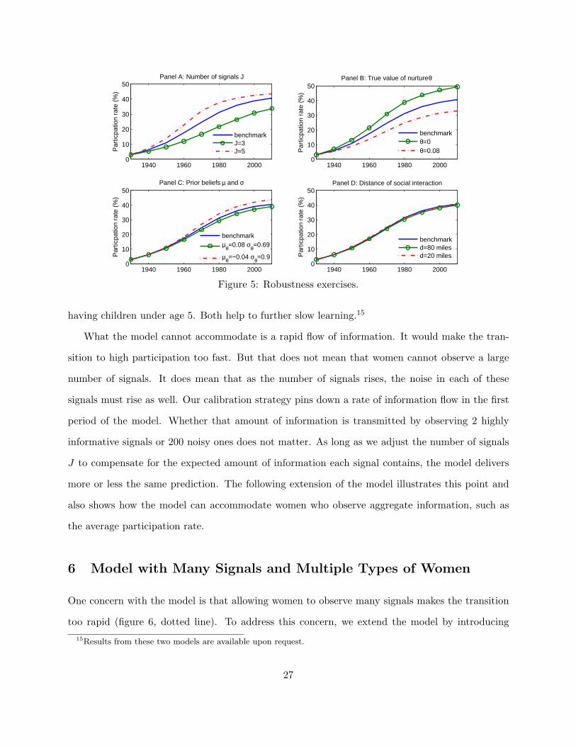
Figure 5 shows that moderate differences in calibrated parameters do not overturn our results.
Increasing the number of signals J speeds the transition but does not change the participation level
that the model converges to (panel A). The exact value of the true θ, even a zero value, has only
a modest effect on the participation rate that the model converges to (panel B). Replacing some
of the initial uncertainty with pessimism (lowering σ, lowering µ0) slows learning initially (panel
C). Even optimism can be offset with initial uncertainty. Furthermore, we can redefine a woman’s
neighborhood d to be within 20-40 miles, with no perceptible differences in the results (panel D).
Finally, feeding the time series of wages in to the model has a negligible effect. Wage-based theories
rely on mechanisms that raise labor supply elasticity to make wages matter. Our model has no
such mechanism.
We have also explored more significant changes to the model. One extension allows θ to fall
over time. Another changes the model timing: Women spend 25 years growing up and 10 years
26
1940 1960 1980 20000
10
20
30
40
50Panel A: Number of signals J
Par
ticpa
tion
rate
(%
)
1940 1960 1980 20000
10
20
30
40
50Panel B: True value of nurture θ
Par
ticpa
tion
rate
(%
)
1940 1960 1980 20000
10
20
30
40
50Panel C: Prior beliefs µ and σ
Par
ticpa
tion
rate
(%
)
1940 1960 1980 20000
10
20
30
40
50Panel D: Distance of social interaction
Par
ticpa
tion
rate
(%
)
benchmarkJ=3J=5
benchmarkθ=0θ=0.08
benchmarkµθ=0.08 σθ=0.69
µθ=−0.04 σθ=0.9
benchmarkd=80 milesd=20 miles
Figure 5: Robustness exercises.
having children under age 5. Both help to further slow learning.15
What the model cannot accommodate is a rapid flow of information. It would make the tran-
sition to high participation too fast. But that does not mean that women cannot observe a large
number of signals. It does mean that as the number of signals rises, the noise in each of these
signals must rise as well. Our calibration strategy pins down a rate of information flow in the first
period of the model. Whether that amount of information is transmitted by observing 2 highly
informative signals or 200 noisy ones does not matter. As long as we adjust the number of signals
J to compensate for the expected amount of information each signal contains, the model delivers
more or less the same prediction. The following extension of the model illustrates this point and
also shows how the model can accommodate women who observe aggregate information, such as
the average participation rate.
6 Model with Many Signals and Multiple Types of Women
One concern with the model is that allowing women to observe many signals makes the transition
too rapid (figure 6, dotted line). To address this concern, we extend the model by introducing15Results from these two models are available upon request.
27

multiple types of women with different costs of maternal employment. This allows women to
observe many signals, and even aggregate information, and still learn slowly.
The idea is that each type of woman has a different cost θ, and must observe other women of the
same type to learn about their type’s cost. Professionals do not learn from seeing hourly workers.
A female doctor who is on call all night does not learn about her θ from seeing the children of
9-5 workers, and urban mothers face different challenges and costs from rural ones. New research,
magazine articles, or aggregate statistics contain no new information because the average cost of
maternal employment is known. Each woman is now learning about how the cost of maternal
employment for her type of woman differs from the average.
The model setup is the same as the benchmark except that there are many types of women,
indexed by ω. A woman of type ω has a cost of maternal employment θω ∼ N(θ, σ2θ), where the
θ’s are i.i.d. across types. A woman’s type ω is publicly observable. The true cost of maternal
employment for the average woman θ is common knowledge.
Simulation results We use the same calibration as the benchmark model, except that there are
now 5 types of women, with θω’s equally spaced between 0.3 and 0.5. Each woman observes 20
signals and knows that the true mean of θ across all types was 0.4. The results in figure 6 are
similar to those of the benchmark model (figure 3).
1940 1960 1980 20000
10
20
30
40
50
60
70
80Labor Force Participation
1940 1960 1980 20000
1
2
3
4
5
6
7
8Cross−County LFP Dispersion
Model (5 types)DataModel (1 type)
Figure 6: Labor force participation with 20 signals per period. Allowing multiple types of womencancels out the effect of more signals.
The reason that the multi-type version of the model looks so much like the original calibrated
model is that the rate of information flow is the same. While women observe 20 signals, on average,
only 4 are relevant for inferring their θω. The other 16 signals are not useful because they are about
28

other types of women. The more general point here is that the number if signals is not crucial for
the model’s results. Instead, the rate of information flow is the key. Our calibration procedure pins
down a rate of information flow by matching the speed of learning in the beginning of the sample.
A model with many noisy signals or few informative ones will generate similar results as long as it
implies a rate of information flow that is in line with the data.
Of course, this leaves open the question of why the rate of information flow is so low. Many
recent theories that use local learning (Amador and Weill (2006), Buera, Monge-Naranjo, and
Primiceri (2006)), rational inattention (Sims 2003), or information generated by economic activity
(Veldkamp (2005), Kurlat (2009)) all require a meager rate of information flow to match the data.
Future work could explore frictions that slow Bayesian learning. Perhaps, social heterogeneity
makes inference from others’ experiences difficult and slows down social learning.
7 Conclusion
Many factors have contributed to the increase in female labor force participation over the last
century. We do not argue that beliefs were the only relevant one. Rather, the model abstracts from
other changes to focus on how the transition from low to high participation can be regulated by
learning in a way that matches the time-series and geographic data. Including local information
transmission as part of the story of female labor force participation in the 20th century helps to
explain its gradual dynamic and geographic evolution.
This framework can be applied to study the geography of other types of economic and social
change. One example is women’s career choice. Suppose that a high-intensity career for a mother
brings with it a higher wage, but also more uncertain effects on children. Since the high-intensity
career is more uncertain than a regular career, fewer women choose it early on. As more women
choose high-intensity careers, others learn from them and the composition of careers changes. The
growth in the fraction of employed women participating in high-intensity careers increases the
average wage of working women. This could be one component of the explanation for a rise in
female wages and its geographic patterns.
29

Clearly, these social transformations involve a change in culture. Rather than seeing cultural
change as a competing explanation, we see this framework as one that can potentially capture
some of the flavor of cultural change. One way to view this paper is as a theory of information
diffusion can change preferences. Another important feature of social behavior is the desire to fit
in or coordinate with others. Using an objective function like that in beauty contest games (Morris
and Shin 2002), coupled with the geographic nature of information transmission, could provide a
rich set of testable implications. Specifically, it could predict geographic patterns, like the spread
from urban to rural areas, in the types of cultural changes investigated by Greenwood and Guner
(2005), Guiso, Sapienza, and Zingales (2006) and Bisin and Verdier (2001). Such work could help
differentiate exogenous changes in preferences from information-driven changes in coordination
outcomes.
Another direction one could take this model is to interpret the concept of distance more broadly.
Arguably, socioeconomic, ethnic, religious or educational differences create stronger social barriers
between people than physical distance does. If that is the case, the learning dynamics that arise
within each social group may be quite distinct. If the initial conditions in these social groups differ,
changes in labor force participation, career choice, or social norms may arise earlier in one group
than in another. This model provides a vehicle for thinking about the diffusion of new behaviors,
with uncertain consequences, among communities of people.
30

References
Albanesi, S., and C. Olivetti (2007): “Gender Roles and Medical Progress,” NBER WorkingPaper 13179.
Alesina, A., and P. Giuliano (2007): “The Power of the Family,” NBER Working Paper 13051.
Amador, M., and P.-O. Weill (2006): “Learning from Private and Public Observations ofOthers’ Actions,” Working Paper.
Antecol, H. (2000): “An Examination of Cross-Country Differences in the Gender Gap in LaborForce Participation Rates,” Labour Economics, 7, 409–426.
Arellano, M., and S. Bond (1991): “Some Tests of Specification for Panel Data: Monte CarloEvidence and an Application to Employment Equations,” Review of Economic Studies, 58(2),277–97.
Attanasio, O., H. Low, and V. Sanchez-Marcos (2008): “Explaining Changes in FemaleLabour Supply in a Life-Cycle Model,” American Economic Review, forthcoming.
Bernal, R., and M. Keane (2006): “Child Care Choices and Childrens Cognitive Achievement:The Case of Single Mothers,” Northwestern University, Working Paper.
Bisin, A., and T. Verdier (2001): “The Economics of Cultural Transmission and the Evolutionof Preferences,” Journal of Economic Theory, 97(2), 298–319.
Buera, F., A. Monge-Naranjo, and G. Primiceri (2006): “Learning the Wealth of Nations,”Northwestern University working paper.
Cover, T., and J. Thomas (1991): Elements of Information Theory. John Wiley and Sons, NewYork, New York, first edn.
Del Boca, D., and D. Vuri (2007): “The Mismatch between labor supply and child care,”Journal of Population Economics, 4.
Farre, L., and F. Vella (2007): “The Intergenerational Transmission of Gender Role Attitudesand its Implications for Female Labor Force Participation,” Georgetown Working Paper.
Fernandez, R. (2007): “Culture as Learning: The Evolution of Female Labor Force Participationover a Century,” Working paper.
Fernandez, R., and A. Fogli (2005): “An Empirical Investigation of Beliefs, Work and Fertility,”NBER Working Paper 11268.
Fernandez, R., A. Fogli, and C. Olivetti (2004): “Mothers and Sons: Preference Formationand Female Labor Force Dynamics,” Quarterly Journal of Economics, 119(4), 1249–1299.
Fortin, N. (2005): “Gender Role Attitudes and the Labor Market Outcomes of Women AcrossOECD Countries,” Oxford Review of Economic Policy, 21, 416–438.
Fuchs-Schundeln, N., and R. Izem (2007): “Explaining the Low Labor Productivity in EastGermany - A Spatial Analysis,” Harvard University Working Paper.
31

Goldin, C. (1990): Understanding the Gender Gap. Oxford University Press.
(1995): “The U-shaped Female Labor Force Function in Economic Development andEconomic History,” in Investment in Human Capital, ed. by T. P. Schultz. University of ChicagoPress.
Goldin, C., and L. Katz (1999): “The Returns to Skill in the United States across the TwentiethCentury,” NBER Working Paper # 7126.
(2002): “The Power of the Pill: Oral Contraceptives and Women’s Career and MarriageDecisions,” Journal of Political Economy, 100, 730–770.
Greenwood, J., and N. Guner (2005): “Social Change,” Economie d’avant gard, researchReport 9, University of Rochester.
Greenwood, J., A. Seshadri, and M. Yorukoglu (2005): “Engines of Liberation,” Review ofEconomic Studies, 72(1), 109–133.
Guiso, L., P. Sapienza, and L. Zingales (2006): “Does Culture Affect Economic Outcomes?,”Journal of Economic Perspecitves, 20(2), 23–48.
Harvey, E. (1999): “Short-Term and Long-Term Effects of Early Parental Employment on Chil-dren of the National Longitudinal Survey of Youth,” Developmental Psychology, 35(2), 445–459.
Hill, J., J. Waldfogel, J. Brooks-Gunn, and W. Han (2005): “Maternal Employment andChild Development: A Fresh Look Using Newer Methods,” Developmental Psychology, 41(6),833–850.
Hobijn, B., and D. Comin (2009): “An Exploration of Technology Diffusion,” HBS WorkingPaper.
Jones, L., R. Manuelli, and E. McGrattan (2003): “Why Are Married Women Working SoMuch?,” Research Department Staff Report 317, Federal Reserve Bank of Minneapolis.
Jovanovic, B. (2009): “The Technology Cycle and Inequality,” Review of Economic Studies,forthcoming, Research Department Staff Report 317, Federal Reserve Bank of Minneapolis.
Kurlat, P. (2009): “Lemons, Market Shutdowns and Learning,” MIT working paper.
Lucas, R. (1972): “Expectations and the Neutrality of Money,” Journal of Economic Theory,4(2), 103–124.
Mammen, K., and C. Paxson (2000): “Women’s Work and Economic Development,” Journal ofEconomic Perspectives, 14(4), 141–164.
Manski, C. (1993): “Identification of Endogenous Social Effects: The Reflection Problem,” TheReview of Economic Studies,, 60(3), 531–542.
Moran, P. (1950): “Notes on continuous stochastic phenomena,” Biometrika, 37, 17–23.
Morris, S., and H. Shin (2002): “The Social Value of Public Information,” American EconomicReview, 92, 1521–1534.
32
Munshi, K. (2004): “Social Learning in a Heterogeneous Population: Technology Diffusion in theIndian Green Revolution,” Journal of Development Economics, 73, 185–213.
Olivetti, C. (2006): “Changes in Women’s Hours of Market Work: The Effect of ChangingReturns to Experience,” Review of Economic Dynamics, 9, 557–587.
O’Neill, J. (1984): “The Trend in the Male-Female Wage Gap in the United States,” Journal ofLabor Economics, 3(1), S91–S116.
Sims, C. (2003): “Implications of Rational Inattention,” Journal of Monetary Economics, 50(3),665–90.
Veldkamp, L. (2005): “Slow Boom, Sudden Crash,” Journal of Economic Theory, 124(2), 230–257.
33

Nature or Nurture: Appendix
A Proofs of analytical results
A.1 Derivation of comparative statics
Step 1: Define a cutoff wage w such that all women who observe wi,t > w choose to join the labor force. Awoman joins the labor force when EUWit − EUOit > 0. Note that ∂Ni,t/∂wit = (nitwit + ωit)−γ > 0.Since Ni,t is monotonically increasing in the wage w, there is a unique w for each set of parameters, suchthat at w = w, Ni,t = 0.Step 2: Describe the probability of labor force participation. Let Φ denote the cumulative density functionfor the unconditional distribution of wages in the population. This is a log-normal c.d.f. Since thelognormal is unbounded and has positive probability on every outcomes, its c.d.f. is therefore strictlyincreasing in its argument. Then, the probability that a woman participates is 1− Φ(w), which is thenstrictly decreasing in w.Step 3: The effect of mean beliefs on labor force participation. Taking the partial derivative of the netutility gain from labor force participation yields ∂Ni,t/∂µi,t = −β. By the implicit function theorem,∂w/∂µi,t > 0. Thus, ∂(1− Φ(w))/∂µi,t = (∂(1− Φ(w))/∂w)(∂w/∂µi,t) < 0.Step 4: Calculate the effect of uncertainty on labor force participation. The benefit to participating isfalling in uncertainty: ∂Ni,t/∂σi,t = (1− γ)β exp
((µa − µi,t)(1− γ) + 1
2 (σ2a + σ2
i,t)(1− γ)2). Since γ > 1,
β > 0 by assumption, and the exponential term must be non-negative, this means that ∂Ni,t/∂σ2i,t < 0. As
before, the implicit function theorem tells us that ∂w/∂σ2i,t > 0. Thus,
∂(1− Φ(w))/∂σ2i,t = (∂(1− Φ(w))/∂w)(∂w/∂σ2
i,t) < 0.
A.2 Proof of result 1: Zero participation is not a steady state
Proof: For any arbitrary beliefs µjt, σjt and endowment ωjt, there is some finite level of ability a∗ and anassociated wage w∗ = exp(a∗), such that EUWit > EUOit > 0, ∀ajt ≥ a∗. The fact that ajt is normallydistributed means that Prob(ajt ≥ a∗) > 0 for all finite a∗. Since woman j enters the labor force wheneverEUWit > EUOit > 0, and this happens with positive probability, njt = 1 with positive probability. Sincethis is true for all women j, it is also true that
∑j njt ≥ 1 with positive probability.
A.3 Proof of result 2: Geographic correlation
Let α be the fraction of women who participate in family i’s region. The region a woman lives in does notaffect her endowments or ability. Therefore, Ni,t+1 can be rewritten, using (7) and (8) as
Ni,t+1 = A−B exp{(γ − 1)µi,t+1 +12(γ − 1)2σ2
i,t+1}
for positive constants A and B. Since woman born at time t participates if Ni,t+1 > 0, if suffices to showthat ∂Ni,t+1/∂α > 0, for a woman with average prior beliefs and an average signal.The number of informative signals that a woman in family i, with an average signal draw, would see isnit = αJ . Since beliefs and signals are unbiased by construction, then a woman with average prior beliefshas µit = θ and a woman with an average signal has µit = θ. By equation (4), her posterior belief isµi,t+1 = θ, for any fraction α. Her posterior precision does depend on α: According to equation 5, thedefinition of σ2
i,t+1, and the equation for nit above, σ−2i,t+1 = σ−2
i,t + αJ/σa. Since J and σa are bothpositive, posterior precision is increasing in α. Thus, posterior variance σ2
i,t+1 is decreasing in α, and Ni,t+1
is increasing in α.
i

B Data: Sources and Definitions
County-level data Our county level dataset has information on a vast array of economic andsocio-demographic variables for 3074 US counties over the period 1940-2000 for each decade. Most of theinformation comes from Census data, and in particular from a dataset called “Historical, Demographic,Economic, and Social Data: The United States, 1790-2000” produced by the Inter-university Consortiumfor Political and Social Research (series 2896). This data set is a consistency-checked and augmentedversion of the the Integrated Public Use Microdata series, produced by the Minnesota Population Center.We integrated this dataset using several others, including the Census of Population and Housing, theCounty and City Data Book, the Census 2000 Summary Files, and IPUMS to obtain the most completeand homogeneous information at the county level for this span of time. Sources and details about theconstruction of each single variable are presented in the on-line appendix.
Benchmark regression Our measures of dispersion and spatial correlation among county levelparticipation rates are calculated on the residuals from the year by year regressionLFPit = β1t + β2tcontrolsit + εit, where the list of controls includes: population density, average education,a set of dummies for type of place (percentage urban, percentage rural farm and percentage rural nonfarm), a set of dummies to capture demographic composition (pecentage white, percentage black andpercentage from other races), and a set of dummies for industrial composition (percentage ofestablishments that are retail, services, manufacturing and wholesales.One data issue we were concerned with was potential bias in our estimates from excluding counties withmissing data. For this reason, we did not include manufacturing wages among the controls, since theinformation on wages is missing for a relevant number of counties in several years. Including wages,however, does not substantially alter our results. We also miss the industrial composition for severalcounties in 1940 and in particularly in the year 2000. We therefore re-calculate the residuals from theregression in the year 2000 excluding sectoral composition from the controls and find that the spatialcorrelation measure rises from 0.38 to 0.45. It is possible that the spatial correlation increases because ofspatial correlation in industrial sector composition that is now attributed to information. However, thecorrelation does not rise (in the first two significant digits) in the previous decades when industrial sectorsare excluded. This suggests that the change in correlation is prevalently due to the sparser data availablein 2000. Therefore, we use the higher estimate, on the full sample of counties, as our measure of spatialcorrelation in the year 2000 in figure 3.
Combining county and national data We use two data sources to construct the labor forceparticipation series: The Integrated Public Use Microdata series (IPUMS) provides information aboutindividuals’ participation decision, along with characteristics such as marital status and presence ofchildren under five years of age. But it does not contain county-level geographic identifiers. The Historical,Demographic, Economic and Social data set (HDES) allows us to compute participation rates by county,but only for all women over the age of 16. Since our theory focuses on the geographic patterns ofparticipation of married mothers of young children, we need to use both sources to approximate the serieswe need.We first use the IPUMS data to calculate an adjustment factor for converting participation rates for allwomen over 16 years to participation rates for white, married women, aged 25-35, with a child under 5 yearsof age, not living on a farm or in an institution. We report the time series of the labor force participationof these two different samples of women in columns 2 and 3 of table 3. We calculate the adjustment factorfor each decade as the ratio between these two columns. We then apply this adjustment factor to convert,decade by decade, each county’s participation rate for all women in that county’s participation rate formothers with children under 5. Finally, to control for economic and demographic differences acrosscounties, we regress this county-level participation on our county-level control variables. The residuals fromthis regression form the data series that we use to compare with the geographic features of the model.To check for consistency between our two data sets, we compared the population-weighted average
ii

source: HDES IPUMS IPUMSsample: all> 16 all> 16 white, 25-35, non-farm
married with kid< 51940 25.3 25.8 6.71950 28.8 29.1 9.81960 35.1 35.7 16.91970 41.2 41.3 24.11980 49.7 49.9 41.51990 56.6 56.7 59.32000 57.1 57.5 59.6
Table 3: Female labor force participation rate, by decade, from various data sources and populationsamples.
participation rate for all women (over 16 years) in all counties from the HDES data with the equivalentseries from IPUMS. Columns 1 and 2 of table 3 show that the two sources report almost identicalaggregate participation rates.
C Calibration
Throughout, we look at women 25-54, with their own child younger than 5 living in the household. We usewhites not living in an institution or on a farm and not working in agriculture.
Abilities The distribution of women’s abilities is constructed so that their wages in the model match thedistribution of women’s wages in the 1940 census data. σa = .57 is the standard deviation of logability and µa = ln(earnings gap)− (σ2
a)/2 is the mean of log ability. These parameters target theinitial ratio between average earnings of working women and average earnings of all husbands (0.81 inthe data) and target the standard deviation of log earnings of employed women in the data (0.53).A wage gap where women earn 81% of their husbands’ income is higher than most estimates. This isdue to two factors. First, we do not require husbands to be full-time workers because we want tocapture the reality that women’s endowments can be high or low. Second, poor women are morelikely to be employed. By comparing only husbands of employed women to their wives, we areselecting poorer husbands.
Selection effects in the model The distribution of observed wages in the data needs to be matchedwith the distribution of wages for employed women in the model. Employed women are not arepresentative sample. They are disproportionately high-skill women. The calibration deals with thisissue by matching the truncated distribution of wages in the data to the same truncated sample inthe model. In other words, we use the model to back out how much selection bias there is.
Endowment distribution The census provides husbands’ wages, starting in 1940. We select out onlyhusbands with children under 5. In the model, the log endowment is normal. Therefore, we examinethe log of 1940 wages. For husbands, mean(log incwage husb ) = 7.04 and std(log incwage husb)= 0.73. Therefore, we set σω = 0.73. We normalize the mean husband’s endowment to 1 by choosingµω = −(σ2
ω)/2.
True value of nurture To calibrate the θ parameter, we use micro evidence on the effect of maternalemployment on the future earnings of children. Our evidence on the effect of maternal employmentcomes from the National Longitudinal Survey of Youth (NLSY), in particular the Peabody PictureVocabulary Test (PPVT) at age 4 and the Peabody Individual Achievement Test (PIAT) for mathand reading recognition scores measured at age 5 and 6. One year of full time maternal employment
iii
plus informal day care reduces test scores by roughly 3.4% (Bernal and Keane 2006). If a motherworks from one year after birth until age six, these five years of employment translate in to a scorereduction of 17%.The childhood test scores are significantly correlated with educational attainment at 18. A 1%increase in the math at age 6 is associated with .019 years of additional schooling. A 1% increase inthe reading test score at age 6 is associated with .025 additional school years. Therefore, five years ofmaternal employment translates into between 0.32 (17*.019) and 0.42 (17*.025) fewer years ofschool.The final step is to multiply the change in educational attainment by the returns to a collegeeducation. We use the returns to a year of college from 1940 to 1995 from Goldin and Katz (1999).Their estimates are the composition-adjusted log weekly wage for full-time/full-year, nonagricultural, white males. Those estimates are 0.1, 0.077, 0.091, 0.099, 0.089, 0.124, and 0.129 for theyears 1939, 1949, 1959, 1969, 1979, 1989, and 1995. The average return to a year of college is 10%.Since maternal employment reduces education by 0.32-0.42 years, the expected loss in terms offoregone yearly log earnings is about 4%, or θ = 0.04.
Number of signals J is calibrated to get the aggregate labor force participation to rise from 6% in 1940to 10% in 1950. Note that this is really pinning down a rate of information flow, rather than anumber of signals. If signals had twice as much noise, but women observed twice as many of them,such a model could match this same calibration target.
Initial Participation in 1930 (heterogeneous across regions) We want to preserve some of thespatial information in our data. However, the model is on a square grid. Mapping irregular-sized UScounties onto this grid is a challenge. To do this, we used regions, which are larger than counties.Regions are constructed by taking the 48 contiguous states, computing the county centroid with thehighest and the lowest longitude (call the difference between the maximum and minimum lodist),and dividing the US map into n vertical strips, each with width lodist/n. Then, for each strip, wecompute the maximum and minimum latitude, and divide the strip into n boxes of equal height. Wechoose n = 10 because it is the largest possible number that does not result in there being boxescontaining no county centroids.In the model, we divide the evenly-spaced agents into 100 regions of equal size and population. Foreach of these 100 regions, we assign the participation rate of the corresponding box on the U.S. mapand assign agents randomly to participate or not. Each participates with a probability given by theregional participation rate. After calibrating initial participation, this regional aggregation structureis never used again and we compute statistics at the more local, county level.
D Model with Learning from Others’ Choices
To keep the model simple and tractable, we assumed that women do not draw any inference from the labordecisions of other women. They use the knowledge of whether J of their peers were nurtured in order toestimate the cost of maternal employment. But they do not take advantage of the fact that the mother’semployment decision reveals something about the mother’s beliefs, which is additional information aboutthe true value of nurture θ.This section shows that our simplifying assumption is innocuous. Seeing other women’s labor forcedecisions does not significantly speed up learning for five reasons: 1) Participation is a binary choice. Thebinary nature of the signal eliminates much of its information. 2) Early on, most women do not work andother women expect that the women they encounter will likely not work. Therefore, a woman who observesanother woman not working early in the century gets very little new (unexpected) information. Observingworking women is informative but it becomes commonplace only later in the century when most of thelearning has been completed. 3) Women observe the participation decisions of women from the previouscohort. Those women were less informed and less likely to work. 4) The “noise” in women’s participationdecisions is large. Women don’t know others’ ability, don’t know whether the mother was nurtured, and
iv

don’t know how uncertain they were. Through all this noise, the belief about the mean is a weak signal. 5)The beliefs of others in your region are highly correlated with your own beliefs because people in the sameregion see common signals. A correlated signal contains less information than an independent one.To quantify these claims, we simulate an economy that is an approximation to the economy where womenlearn from the decisions of other women. To keep the linear Bayesian updating rules, we consider aneconomy where women observe additional normally distributed signals whose signal-to-noise ratio is thesame as the information embedded in the participation decisions they observe. This is an upper bound onhow much additional information comes from others’ decisions because normally distributed signals containmore information than any other kind of signal with the same signal-to-noise ratio (Cover andThomas 1991).To estimate the signal-to-noise ratio of women’s employment decisions, run a regression of participation onbeliefs. Since the informativeness of women’s labor decisions changes over time, there should be a separateregression run for each decade. Compute the R2. The signal-to-noise ratio, the ratio of the explained sumof squares (signal) to unexplained (noise), is R2/(1−R2). To construct a signal with the same amount ofnoise, first compute the cross-sectional variance of women’s beliefs. This is the total sum of squares.Multiply this variance by 1−R2 to get the unexplained sum of squares. Create an m× 1 vector of i.i.d.normal random variables with mean zero and variance (1−R2)var(µt), where m is the number of womenin the economy. Add this noise shock to the vector of women’s beliefs. Each woman in generation t + 1 seesa subset of the signals about generation t beliefs, where the subset is the signals with indices jεJi.
1940 1960 1980 20000
20
40
60
80Labor Force Participation
1940 1960 1980 20000
2
4
6
8Cross−County LFP Dispersion
ModelData
Figure 7: Labor force participation when women observe participation decisions of others.
The time-series of labor force participation that results from simulating this model, with the samecalibrated parameters as in table 1 of the main text, appears in figure 7. This approach generates a laborforce participation rate that is only 5% higher at the end of the sample. Thus, learning from other women’sparticipation choices does speed up the increase in labor force participation by speeding up learning, butits effect is small.
v