Natural Scene Statistics Account for the …amygdala.psychdept.arizona.edu/Jclub/Natural-scenes+2013.pdfNeuron Article Natural Scene Statistics Account for the Representation of Scene

Neuron

Article

Natural Scene Statistics Accountfor the Representation of Scene Categoriesin Human Visual CortexDustin E. Stansbury,1 Thomas Naselaris,2,4 and Jack L. Gallant1,2,3,*1Vision Science Group2Helen Wills Neuroscience Institute3Department of PsychologyUniversity of California, Berkeley, CA 94720, USA4Present address: Department of Neurosciences, Medical University of South Carolina, Charleston, SC 29425, USA

*Correspondence: [email protected]

http://dx.doi.org/10.1016/j.neuron.2013.06.034

SUMMARY

During natural vision, humans categorize the scenesthey encounter: an office, the beach, and so on.These categories are informed by knowledge ofthe way that objects co-occur in natural scenes.How does the human brain aggregate informationabout objects to represent scene categories? Toexplore this issue, we used statistical learningmethods to learn categories that objectively capturethe co-occurrence statistics of objects in a largecollection of natural scenes. Using the learnedcategories, we modeled fMRI brain signals evokedin human subjects when viewing images ofscenes. We find that evoked activity across muchof anterior visual cortex is explained by the learnedcategories. Furthermore, a decoder based on thesescene categories accurately predicts the categoriesand objects comprising novel scenes from brainactivity evoked by those scenes. These results sug-gest that the human brain represents scene cate-gories that capture the co-occurrence statistics ofobjects in the world.

INTRODUCTION

During natural vision, humans categorize the scenes that they

encounter. A scene category can often be inferred from the

objects present in the scene. For example, a person can infer

that she is at the beach by seeing water, sand, and sunbathers.

Inferences can also be made in the opposite direction: the cate-

gory ‘‘beach’’ is sufficient to elicit the recall of these objects

plus many others such as towels, umbrellas, sandcastles, and

so on. These objects are very different from those that would

be recalled for another scene category such as an office. These

observations suggest that humans use knowledge about how

objects co-occur in the natural world to categorize natural

scenes.

Ne

There is substantial behavioral evidence to show that humans

exploit the co-occurrence statistics of objects during natural

vision. For example, object recognition is faster when objects

in a scene are contextually consistent (Biederman, 1972; Bieder-

man et al., 1973; Palmer, 1975). When a scene contains objects

that are contextually inconsistent, then scene categorization is

more difficult (Potter, 1975; Davenport and Potter, 2004; Joubert

et al., 2007). Despite the likely importance of object co-occur-

rence statistics for visual scene perception, few fMRI studies

have investigated this issue systematically. Most previous fMRI

studies have investigated isolated and decontextualized objects

(Kanwisher et al., 1997; Downing et al., 2001) or a few, very broad

scene categories (Epstein and Kanwisher, 1998; Peelen et al.,

2009). However, two recent fMRI studies (Walther et al., 2009;

MacEvoy and Epstein, 2011) provide some evidence that the

human visual system represents information about individual

objects during scene perception.

Here we test the hypothesis that the human visual system

represents scene categories that capture the statistical rela-

tionships between objects in the natural world. To investigate

this issue, we used a statistical learning algorithm originally

developed to model large text corpora to learn scene cate-

gories that capture the co-occurrence statistics of objects

found in a large collection of natural scenes. We then used

fMRI to record blood oxygenation level-dependent (BOLD)

activity evoked in the human brain when viewing natural

scenes. Finally, we used the learned scene categories to model

the tuning of individual voxels and we compared predictions

of these models to alternative models based on object co-

occurrence statistics that lack the statistical structure inherent

in natural scenes.

We report three main results that are consistent with our

hypothesis. First, much of anterior visual cortex represents

scene categories that reflect the co-occurrence statistics of

objects in natural scenes. Second, voxels located within and

beyond the boundaries of many well-established functional

ROIs in anterior visual cortex are tuned to mixtures of these

scene categories. Third, scene categories and the specific

objects that occur in novel scenes can be accurately decoded

from evoked brain activity alone. Taken together, these results

suggest that scene categories represented in the human brain

uron 79, 1025–1034, September 4, 2013 ª2013 Elsevier Inc. 1025

mailto:[email protected]


http://crossmark.dyndns.org/dialog/?doi=10.1016/j.neuron.2013.06.034&domain=pdf

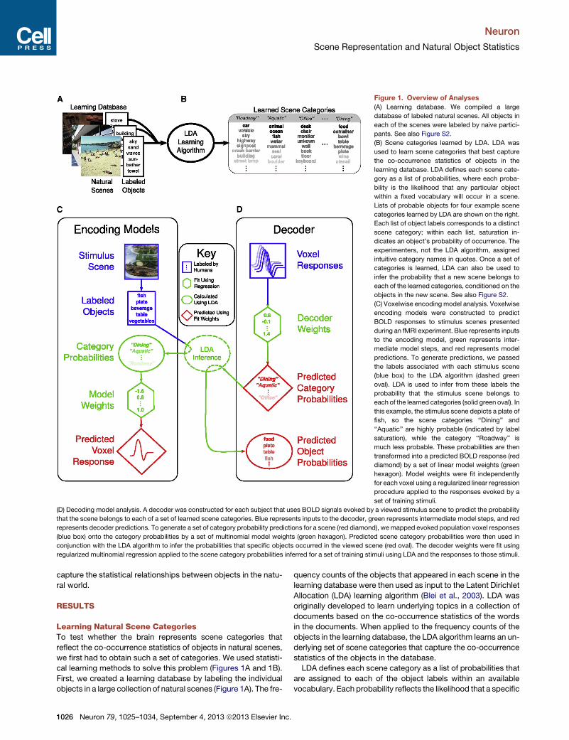
Figure 1. Overview of Analyses

(A) Learning database. We compiled a large

database of labeled natural scenes. All objects in

each of the scenes were labeled by naive partici-

pants. See also Figure S2.

(B) Scene categories learned by LDA. LDA was

used to learn scene categories that best capture

the co-occurrence statistics of objects in the

learning database. LDA defines each scene cate-

gory as a list of probabilities, where each proba-

bility is the likelihood that any particular object

within a fixed vocabulary will occur in a scene.

Lists of probable objects for four example scene

categories learned by LDA are shown on the right.

Each list of object labels corresponds to a distinct

scene category; within each list, saturation in-

dicates an object’s probability of occurrence. The

experimenters, not the LDA algorithm, assigned

intuitive category names in quotes. Once a set of

categories is learned, LDA can also be used to

infer the probability that a new scene belongs to

each of the learned categories, conditioned on the

objects in the new scene. See also Figure S2.

(C) Voxelwise encoding model analysis. Voxelwise

encoding models were constructed to predict

BOLD responses to stimulus scenes presented

during an fMRI experiment. Blue represents inputs

to the encoding model, green represents inter-

mediate model steps, and red represents model

predictions. To generate predictions, we passed

the labels associated with each stimulus scene

(blue box) to the LDA algorithm (dashed green

oval). LDA is used to infer from these labels the

probability that the stimulus scene belongs to

each of the learned categories (solid green oval). In

this example, the stimulus scene depicts a plate of

fish, so the scene categories ‘‘Dining’’ and

‘‘Aquatic’’ are highly probable (indicated by label

saturation), while the category ‘‘Roadway’’ is

much less probable. These probabilities are then

transformed into a predicted BOLD response (red

diamond) by a set of linear model weights (green

hexagon). Model weights were fit independently

for each voxel using a regularized linear regression

procedure applied to the responses evoked by a

set of training stimuli.

(D) Decoding model analysis. A decoder was constructed for each subject that uses BOLD signals evoked by a viewed stimulus scene to predict the probability

that the scene belongs to each of a set of learned scene categories. Blue represents inputs to the decoder, green represents intermediate model steps, and red

represents decoder predictions. To generate a set of category probability predictions for a scene (red diamond), we mapped evoked population voxel responses

(blue box) onto the category probabilities by a set of multinomial model weights (green hexagon). Predicted scene category probabilities were then used in

conjunction with the LDA algorithm to infer the probabilities that specific objects occurred in the viewed scene (red oval). The decoder weights were fit using

regularized multinomial regression applied to the scene category probabilities inferred for a set of training stimuli using LDA and the responses to those stimuli.

Neuron

Scene Representation and Natural Object Statistics

capture the statistical relationships between objects in the natu-

ral world.

RESULTS

Learning Natural Scene CategoriesTo test whether the brain represents scene categories that

reflect the co-occurrence statistics of objects in natural scenes,

we first had to obtain such a set of categories. We used statisti-

cal learning methods to solve this problem (Figures 1A and 1B).

First, we created a learning database by labeling the individual

objects in a large collection of natural scenes (Figure 1A). The fre-

1026 Neuron 79, 1025–1034, September 4, 2013 ª2013 Elsevier Inc.

quency counts of the objects that appeared in each scene in the

learning database were then used as input to the Latent Dirichlet

Allocation (LDA) learning algorithm (Blei et al., 2003). LDA was

originally developed to learn underlying topics in a collection of

documents based on the co-occurrence statistics of the words

in the documents. When applied to the frequency counts of the

objects in the learning database, the LDA algorithm learns an un-

derlying set of scene categories that capture the co-occurrence

statistics of the objects in the database.

LDA defines each scene category as a list of probabilities that

are assigned to each of the object labels within an available

vocabulary. Each probability reflects the likelihood that a specific

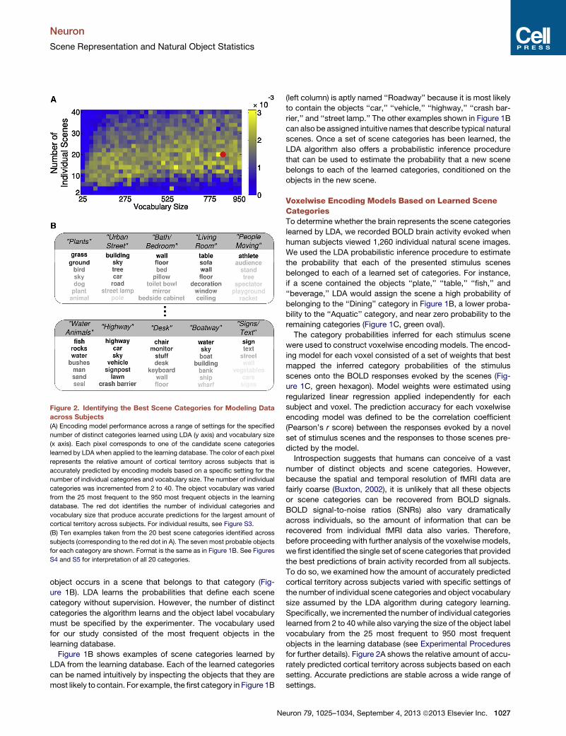
Figure 2. Identifying the Best Scene Categories for Modeling Data

across Subjects

(A) Encoding model performance across a range of settings for the specified

number of distinct categories learned using LDA (y axis) and vocabulary size

(x axis). Each pixel corresponds to one of the candidate scene categories

learned by LDA when applied to the learning database. The color of each pixel

represents the relative amount of cortical territory across subjects that is

accurately predicted by encoding models based on a specific setting for the

number of individual categories and vocabulary size. The number of individual

categories was incremented from 2 to 40. The object vocabulary was varied

from the 25 most frequent to the 950 most frequent objects in the learning

database. The red dot identifies the number of individual categories and

vocabulary size that produce accurate predictions for the largest amount of

cortical territory across subjects. For individual results, see Figure S3.

(B) Ten examples taken from the 20 best scene categories identified across

subjects (corresponding to the red dot in A). The seven most probable objects

for each category are shown. Format is the same as in Figure 1B. See Figures

S4 and S5 for interpretation of all 20 categories.

Neuron


object occurs in a scene that belongs to that category (Fig-

ure 1B). LDA learns the probabilities that define each scene

category without supervision. However, the number of distinct

categories the algorithm learns and the object label vocabulary

must be specified by the experimenter. The vocabulary used

for our study consisted of the most frequent objects in the

learning database.

Figure 1B shows examples of scene categories learned by

LDA from the learning database. Each of the learned categories

can be named intuitively by inspecting the objects that they are

most likely to contain. For example, the first category in Figure 1B

Ne

(left column) is aptly named ‘‘Roadway’’ because it is most likely

to contain the objects ‘‘car,’’ ‘‘vehicle,’’ ‘‘highway,’’ ‘‘crash bar-

rier,’’ and ‘‘street lamp.’’ The other examples shown in Figure 1B

can also be assigned intuitive names that describe typical natural

scenes. Once a set of scene categories has been learned, the

LDA algorithm also offers a probabilistic inference procedure

that can be used to estimate the probability that a new scene

belongs to each of the learned categories, conditioned on the

objects in the new scene.

Voxelwise Encoding Models Based on Learned SceneCategoriesTo determine whether the brain represents the scene categories

learned by LDA, we recorded BOLD brain activity evoked when

human subjects viewed 1,260 individual natural scene images.

We used the LDA probabilistic inference procedure to estimate

the probability that each of the presented stimulus scenes

belonged to each of a learned set of categories. For instance,

if a scene contained the objects ‘‘plate,’’ ‘‘table,’’ ‘‘fish,’’ and

‘‘beverage,’’ LDA would assign the scene a high probability of

belonging to the ‘‘Dining’’ category in Figure 1B, a lower proba-

bility to the ‘‘Aquatic’’ category, and near zero probability to the

remaining categories (Figure 1C, green oval).

The category probabilities inferred for each stimulus scene

were used to construct voxelwise encoding models. The encod-

ing model for each voxel consisted of a set of weights that best

mapped the inferred category probabilities of the stimulus

scenes onto the BOLD responses evoked by the scenes (Fig-

ure 1C, green hexagon). Model weights were estimated using

regularized linear regression applied independently for each

subject and voxel. The prediction accuracy for each voxelwise

encoding model was defined to be the correlation coefficient

(Pearson’s r score) between the responses evoked by a novel

set of stimulus scenes and the responses to those scenes pre-

dicted by the model.

Introspection suggests that humans can conceive of a vast

number of distinct objects and scene categories. However,

because the spatial and temporal resolution of fMRI data are

fairly coarse (Buxton, 2002), it is unlikely that all these objects

or scene categories can be recovered from BOLD signals.

BOLD signal-to-noise ratios (SNRs) also vary dramatically

across individuals, so the amount of information that can be

recovered from individual fMRI data also varies. Therefore,

before proceeding with further analysis of the voxelwise models,

we first identified the single set of scene categories that provided

the best predictions of brain activity recorded from all subjects.

To do so, we examined how the amount of accurately predicted

cortical territory across subjects varied with specific settings of

the number of individual scene categories and object vocabulary

size assumed by the LDA algorithm during category learning.

Specifically, we incremented the number of individual categories

learned from 2 to 40 while also varying the size of the object label

vocabulary from the 25 most frequent to 950 most frequent

objects in the learning database (see Experimental Procedures

for further details). Figure 2A shows the relative amount of accu-

rately predicted cortical territory across subjects based on each

setting. Accurate predictions are stable across a wide range of

settings.


Neuron


Across subjects, the encoding models perform best when

based on 20 individual categories and composed of a vocabu-

lary of 850 objects (Figure 2A, indicated by red dot; for individual

subject results, see Figure S3 available online). Examples of

these categories are displayed in Figure 2B (for an interpretation

of all 20 categories, see Figures S4 and S5). To the best of our

knowledge, previous fMRI studies have only used two to eight

distinct categories and 2–200 individual objects (see Walther

et al., 2009; MacEvoy and Epstein, 2011). Thus, our results

show there is more information in BOLD signals related to en-

coding scene categories than has been previously appreciated.

We next tested whether natural scene categories were neces-

sary to accurately model the measured fMRI data. We derived a

set of null scene categories by training LDA on artificial scenes.

The artificial scenes were created by scrambling the objects in

the learning database across scenes, thus removing the natural

statistical structure of object co-occurrences inherent in the orig-

inal learning database. If the brain incorporates information

about the co-occurrence statistics of objects in natural scenes,

then the prediction accuracy of encoding models based upon

these null scene categories should be much poorer than encod-

ing models based on scene categories learned from natural

scenes.

Indeed, we find that encodingmodels based on the categories

learned from natural scenes provide significantly better predic-

tions of brain activity than do encoding models based on the

null categories and for all subjects (p < 13 10�10 for all subjects,

Wilcox rank-sum test for differences in median prediction accu-

racy across all cortical voxels and candidate scene category

settings; subject S1: W(15,025,164) = 9.96 3 1013 ; subject S2:

W(24,440,399) = 3.04 3 1014 ; subject S3: W(15,778,360) =

9.93 3 1013 ; subject S4: W(14,705,625) = 1.09 3 1014). In a

set of supplemental analyses, we also compared the LDA-based

models to several other plausible models of scene category

representation. We find that the LDA-based models provide

superior prediction accuracy to all these alternative models

(see Figures S12–S15). These results support our central hypoth-

esis that the human brain encodes categories that reflect the

co-occurrence statistics of objects in natural scenes.

Categories Learned From Natural Scenes ExplainSelectivity in Many Anterior Visual ROIsPrevious fMRI studies have identified functional regions of inter-

est (ROIs) tuned to very broad scene categories, such as places

(Epstein and Kanwisher, 1998), as well as to narrow object

categories such as faces (Kanwisher et al., 1997) or body parts

(Downing et al., 2001). Can selectivity in these regions be

explained in terms of the categories learned from natural scene

object statistics?

We evaluated scene category tuning for voxels located within

the boundaries of several conventional functional ROIs: the fusi-

form face area (FFA; Kanwisher et al., 1997), the occipital face

area (OFA; Gauthier et al., 2000), the extrastriate body area

(EBA; Downing et al., 2001), the parahippocampal place area

(PPA; Epstein and Kanwisher, 1998), the transverse occipital sul-

cus (TOS; Nakamura et al., 2000; Grill-Spector, 2003; Hasson

et al., 2003), the retrosplenial cortex (RSC; Maguire, 2001), and

lateral occipital cortex (LO; Malach et al., 1995).


Figure 3A shows the boundaries of these ROIs, identified using

separate functional localizer experiments, and projected on the

cortical flat map of one representative subject. The color of

each location on the cortical map indicates the prediction accu-

racy of the corresponding encoding model. All encoding models

were based on the 20 best scene categories identified across

subjects. These data show that the encoding models accurately

predict responses of voxels located in many ROIs within anterior

visual cortex. To quantify this effect, we calculated the propor-

tion of response variance explained by the encoding models,

averaged across all voxels within each ROI. We find that the

average proportion of variance explained to be significantly

greater than chance for every anterior visual cortex ROI and for

all subjects (p < 0.01; see Experimental Procedures for details).

Thus, selectivity in many previously identified ROIs can be

explained in terms of tuning to scene categories learned from

natural scene statistics.

To determinewhether scene category tuning is consistent with

tuning reported in earlier localizer studies, we visualized the

weights of encoding models fit to voxels within each ROI. Fig-

ure 3C shows encoding model weights averaged across all vox-

els located within each function ROI. Scene category selectivity

is broadly consistent with the results of previous functional local-

izer experiments. For example, previous studies have suggested

that PPA is selective for presence of buildings (Epstein and

Kanwisher, 1998). The LDA algorithm suggests that images con-

taining buildings are most likely to belong to the ‘‘Urban/Street’’

category (see Figure 2B), andwe find that voxels within PPA have

large weights for the ‘‘Urban/Street’’ category (see Figures S4

and S5). To take another example, previous studies have sug-

gested that OFA is selective for the presence of human faces

(Gauthier et al., 2000). Under the trained LDA model, images

containing faces are most likely to belong to the ‘‘Portrait’’ cate-

gory (see Figures S4 and S5), and we find that voxels within OFA

have large weights for the ‘‘Portrait’’ category.

Although category tuning within functional ROIs is generally

consistent with previous reports, Figure 3C demonstrates that

tuning is clearly more complicated than assumed previously. In

particular, many functional ROIs are tuned for more than one

scene category. For example, both FFA and OFA are thought

to be selective for human faces, but voxels in both these areas

also have large weights for the ‘‘Plants’’ category. Additionally,

area TOS, an ROI generally associated with encoding informa-

tion important for navigation, has relatively large weights for

the ‘‘Portrait’’ and ‘‘People Moving’’ categories. Thus, our results

suggest that tuning in conventional ROIs may be more diverse

than generally believed (for additional evidence, see Huth

et al., 2012 and Naselaris et al., 2012).

Decoding Natural Scene Categories from Evoked BrainActivityThe results presented thus far suggest that information about

natural scene categories is encoded in the activity of many

voxels located in anterior visual cortex. It should therefore be

possible to decode these scene categories from brain activity

evoked by viewing a scene. To investigate this possibility, we

constructed a decoder for each subject that uses voxel activity

evoked in anterior visual cortex to predict the probability that a

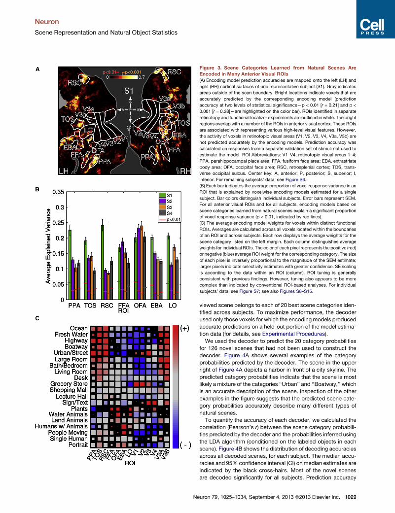
Figure 3. Scene Categories Learned from Natural Scenes Are

Encoded in Many Anterior Visual ROIs

(A) Encoding model prediction accuracies are mapped onto the left (LH) and

right (RH) cortical surfaces of one representative subject (S1). Gray indicates

areas outside of the scan boundary. Bright locations indicate voxels that are

accurately predicted by the corresponding encoding model (prediction

accuracy at two levels of statistical significance—p < 0.01 [r = 0.21] and p <

0.001 [r = 0.28]—are highlighted on the color bar). ROIs identified in separate

retinotopy and functional localizer experiments are outlined inwhite. The bright

regions overlap with a number of the ROIs in anterior visual cortex. These ROIs

are associated with representing various high-level visual features. However,

the activity of voxels in retinotopic visual areas (V1, V2, V3, V4, V3a, V3b) are

not predicted accurately by the encoding models. Prediction accuracy was

calculated on responses from a separate validation set of stimuli not used to

estimate the model. ROI Abbreviations: V1–V4, retinotopic visual areas 1–4;

PPA, parahippocampal place area; FFA, fusiform face area; EBA, extrastriate

body area; OFA, occipital face area; RSC, retrosplenial cortex; TOS, trans-

verse occipital sulcus. Center key: A, anterior; P, posterior; S, superior; I,

inferior. For remaining subjects’ data, see Figure S6.

(B) Each bar indicates the average proportion of voxel response variance in an

ROI that is explained by voxelwise encoding models estimated for a single

subject. Bar colors distinguish individual subjects. Error bars represent SEM.

For all anterior visual ROIs and for all subjects, encoding models based on

scene categories learned from natural scenes explain a significant proportion

of voxel response variance (p < 0.01, indicated by red lines).

(C) The average encoding model weights for voxels within distinct functional

ROIs. Averages are calculated across all voxels located within the boundaries

of an ROI and across subjects. Each row displays the average weights for the

scene category listed on the left margin. Each column distinguishes average

weights for individual ROIs. The color of each pixel represents the positive (red)

or negative (blue) average ROI weight for the corresponding category. The size

of each pixel is inversely proportional to the magnitude of the SEM estimate;

larger pixels indicate selectivity estimates with greater confidence. SE scaling

is according to the data within an ROI (column). ROI tuning is generally

consistent with previous findings. However, tuning also appears to be more

complex than indicated by conventional ROI-based analyses. For individual

subjects’ data, see Figure S7; see also Figures S8–S15.

Neuron


Ne

viewed scene belongs to each of 20 best scene categories iden-

tified across subjects. To maximize performance, the decoder

used only those voxels for which the encoding models produced

accurate predictions on a held-out portion of the model estima-

tion data (for details, see Experimental Procedures).

We used the decoder to predict the 20 category probabilities

for 126 novel scenes that had not been used to construct the

decoder. Figure 4A shows several examples of the category

probabilities predicted by the decoder. The scene in the upper

right of Figure 4A depicts a harbor in front of a city skyline. The

predicted category probabilities indicate that the scene is most

likely a mixture of the categories ‘‘Urban’’ and ‘‘Boatway,’’ which

is an accurate description of the scene. Inspection of the other

examples in the figure suggests that the predicted scene cate-

gory probabilities accurately describe many different types of

natural scenes.

To quantify the accuracy of each decoder, we calculated the

correlation (Pearson’s r) between the scene category probabili-

ties predicted by the decoder and the probabilities inferred using

the LDA algorithm (conditioned on the labeled objects in each

scene). Figure 4B shows the distribution of decoding accuracies

across all decoded scenes, for each subject. The median accu-

racies and 95% confidence interval (CI) on median estimates are

indicated by the black cross-hairs. Most of the novel scenes

are decoded significantly for all subjects. Prediction accuracy


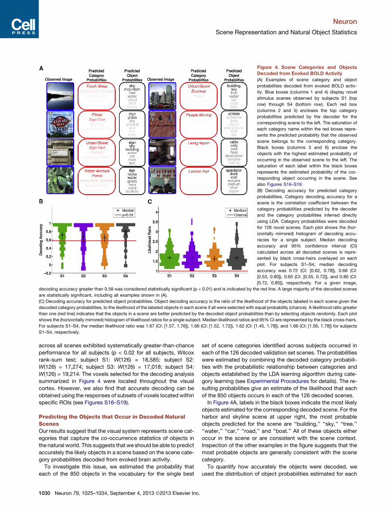
Figure 4. Scene Categories and Objects

Decoded from Evoked BOLD Activity

(A) Examples of scene category and object

probabilities decoded from evoked BOLD activ-

ity. Blue boxes (columns 1 and 4) display novel

stimulus scenes observed by subjects S1 (top

row) through S4 (bottom row). Each red box

(columns 2 and 5) encloses the top category

probabilities predicted by the decoder for the

corresponding scene to the left. The saturation of

each category name within the red boxes repre-

sents the predicted probability that the observed

scene belongs to the corresponding category.

Black boxes (columns 3 and 6) enclose the

objects with the highest estimated probability of

occurring in the observed scene to the left. The

saturation of each label within the black boxes

represents the estimated probability of the cor-

responding object occurring in the scene. See

also Figures S16–S19.

(B) Decoding accuracy for predicted category

probabilities. Category decoding accuracy for a

scene is the correlation coefficient between the

category probabilities predicted by the decoder

and the category probabilities inferred directly

using LDA. Category probabilities were decoded

for 126 novel scenes. Each plot shows the (hor-

izontally mirrored) histogram of decoding accu-

racies for a single subject. Median decoding

accuracy and 95% confidence interval (CI)

calculated across all decoded scenes is repre-

sented by black cross-hairs overlayed on each

plot. For subjects S1–S4, median decoding

accuracy was 0.72 (CI: [0.62, 0.78]), 0.68 (CI:

[0.53, 0.80]), 0.65 (CI: [0.55, 0.72]), and 0.80 (CI:

[0.72, 0.85]), respectively. For a given image,

decoding accuracy greater than 0.58 was considered statistically significant (p < 0.01) and is indicated by the red line. A large majority of the decoded scenes

are statistically significant, including all examples shown in (A).

(C) Decoding accuracy for predicted object probabilities. Object decoding accuracy is the ratio of the likelihood of the objects labeled in each scene given the

decoded category probabilities, to the likelihood of the labeled objects in each scene if all were selected with equal probability (chance). A likelihood ratio greater

than one (red line) indicates that the objects in a scene are better predicted by the decoded object probabilities than by selecting objects randomly. Each plot

shows the (horizontally mirrored) histogram of likelihood ratios for a single subject. Median likelihood ratios and 95%CI are represented by the black cross-hairs.

For subjects S1–S4, the median likelihood ratio was 1.67 (CI: [1.57, 1.76]), 1.66 (CI: [1.52, 1.72]), 1.62 (CI: [1.45, 1.78]), and 1.66 (CI: [1.56, 1.78]) for subjects

S1–S4, respectively.

Neuron


across all scenes exhibited systematically greater-than-chance

performance for all subjects (p < 0.02 for all subjects, Wilcox

rank-sum test; subject S1: W(126) = 18,585; subject S2:

W(126) = 17,274; subject S3: W(126) = 17,018; subject S4:

W(126) = 19,214. The voxels selected for the decoding analysis

summarized in Figure 4 were located throughout the visual

cortex. However, we also find that accurate decoding can be

obtained using the responses of subsets of voxels located within

specific ROIs (see Figures S16–S19).

Predicting the Objects that Occur in Decoded NaturalScenesOur results suggest that the visual system represents scene cat-

egories that capture the co-occurrence statistics of objects in

the natural world. This suggests that we should be able to predict

accurately the likely objects in a scene based on the scene cate-

gory probabilities decoded from evoked brain activity.

To investigate this issue, we estimated the probability that

each of the 850 objects in the vocabulary for the single best


set of scene categories identified across subjects occurred in

each of the 126 decoded validation set scenes. The probabilities

were estimated by combining the decoded category probabili-

ties with the probabilistic relationship between categories and

objects established by the LDA learning algorithm during cate-

gory learning (see Experimental Procedures for details). The re-

sulting probabilities give an estimate of the likelihood that each

of the 850 objects occurs in each of the 126 decoded scenes.

In Figure 4A, labels in the black boxes indicate the most likely

objects estimated for the corresponding decoded scene. For the

harbor and skyline scene at upper right, the most probable

objects predicted for the scene are ‘‘building,’’ ‘‘sky,’’ ‘‘tree,’’

‘‘water,’’ ‘‘car,’’ ‘‘road,’’ and ‘‘boat.’’ All of these objects either

occur in the scene or are consistent with the scene context.

Inspection of the other examples in the figure suggests that the

most probable objects are generally consistent with the scene

category.

To quantify how accurately the objects were decoded, we

used the distribution of object probabilities estimated for each

Neuron


scene to calculate the likelihood of the labeled objects in the

scene. We then calculated the likelihood of the labeled objects

from a naive distribution that assumes all 850 objects are equally

likely to occur. The ratio of these likelihoods provides a measure

of accuracy for the estimated object probabilities. Likelihood ra-

tios greater than one indicate that the estimated object probabil-

ities better predict the labeled objects in the scene than by pick-

ing objects at random (see Experimental Procedures for details).

Figure 4C shows the distribution of likelihood ratios for each

subject, calculated for all 126 decoded scenes. The medians

and 95% confidence intervals of the median estimates are indi-

cated by the black cross-hairs. Object prediction accuracy

across all scenes indicates systematically greater-than-chance

performance for all subjects (p < 1 3 10�15 for all subjects, Wil-

cox rank-sum test; subject S1: W(126) = 9,983; subject S2:

W(126) = 11,375; subject S3: W(126) = 11,103; subject S4:

W(126) = 10,715).

The estimated object probabilities and the likelihood ratio

analysis both show that the objects that are likely to occur in a

scene can be predicted probabilistically from natural scene cat-

egories that are encoded in human brain activity. This suggests

that humans might use a probabilistic strategy to help infer the

likely objects in a scene from fragmentary information available

at any point in time.

DISCUSSION

This study provides compelling evidence that the human visual

system encodes scene categories that reflect the co-occurrence

statistics of objects in the natural world. First, categories that

capture co-occurrence statistics are consistent with our intuitive

interpretations of natural scenes. Second, voxelwise encoding

models based on these categories accurately predict visually

evoked BOLD activity across much of anterior visual cortex,

including within several conventional functional ROIs. Finally,

the category of a scene and its constituent objects can be

decoded from BOLD activity evoked by viewing the scene.

Previous studies of scene representation in the human brain

used subjective categories that were selected by the experi-

menters. In contrast, our study used a data-driven, statistical al-

gorithm (LDA) to learn the intrinsic categorical structure of natural

scenes from object labels. These learned, intrinsic scene cate-

gories provide a more objective foundation for scene perception

research than is possible using subjective categories.

One previous computer vision study used a similar statistical

learning approach to investigate the intrinsic category structure

of natural scenes (Fei-Fei and Perona, 2005). In that study, the

input to the learning algorithm was visual features of interme-

diate spatial complexity. Because our goal was to determine

whether the brain represents the object co-occurrence statistics

of natural scenes, we used object labels of natural scenes as

input to the learning algorithm rather than intermediate visual

features.

The voxelwise modeling and decoding framework employed

here (Kay et al., 2008b; Mitchell et al., 2008; Naselaris et al.,

2009, 2012; Nishimoto et al., 2011; Thirion et al., 2006) provides

a powerful alternative to conventional methods based on statis-

tical parametric mapping (Friston et al., 1996) or multivariate

Ne

pattern analysis (MVPA; Norman et al., 2006). Studies based

on statistical mapping or MVPA do not aim to produce explicit

predictive models of voxel tuning, so it is difficult to generalize

their results beyond the specific stimuli or task conditions used

in each study. In contrast, the goal of voxelwise modeling is to

produce models that can accurately predict responses to arbi-

trary, novel stimuli or task conditions. A key strategy for devel-

oping theoretical models of natural systems has been to validate

model predictions under novel conditions (Hastie et al., 2008).

We believe that this strategy is also critically important for devel-

oping theories of representation in the human brain.

Our results generally corroborate themany previous reports of

object selectivity in anterior visual cortex. However, we find that

tuning properties in this part of visual cortex are more complex

than reported in previous studies (see Figures S7, S8–S11, and

S16–S19 for supporting results). This difference probably

reflects the sensitivity afforded by the voxelwise modeling and

decoding framework. Still, much work remains before we can

claim a complete understanding of what and how information

is represented in anterior visual cortex (Huth et al., 2012; Nase-

laris et al., 2012).

Several recent studies (Kim and Biederman, 2011; MacEvoy

and Epstein, 2011; Peelen et al., 2009) have suggested that the

lateral occipital complex (LO) represents, in part, the identity of

scene categories based on the objects therein. Taken together,

these studies suggest that some subregions within LO should be

accurately predicted by models that link objects with scene cat-

egories. Our study employs one such model. We find that the

encoding models based on natural scene categories provide

accurate predictions of activity in anterior portions of LO (Figures

3A and 3B). Note, however, that our results do not necessarily

imply that LO represents scene categories explicitly (see Figures

S16–S19 for further analyses).

fMRI provides only a coarse proxy of neural activity and has a

low SNR. In order to correctly interpret the results of fMRI exper-

iments, it is important to quantify how much information can be

recovered from these data. Here we addressed this problem

by testing many candidate models in order to determine a single

set of scene categories that can be recovered reliably from the

BOLD activity measured across all of our subjects (Figure 2A).

This test places a clear empirical limit on the number of scene

categories and objects that can be recovered from our data.

These numbers are larger than what has typically been assumed

in previous fMRI studies of scene perception (Epstein and Kanw-

isher, 1998; Peelen et al., 2009; Walther et al., 2009; MacEvoy

and Epstein, 2011), but they are still far smaller than the likely

representational capacity of the human visual system.

Theoreticians have argued that the simple statistical proper-

ties of natural scenes explain selectivity to low-level features in

peripheral sensory areas (Olshausen and Field, 1996; Smith

and Lewicki, 2006). Behavioral data suggest that low-level

natural scene statistics also influence the perception of scene

categories (Oliva and Torralba, 2001; Torralba and Oliva,

2003). Though several qualitative theories have been proposed

that link the object statistics of natural scenes with human scene

perception (Biederman, 1981; Palmer, 1975), none have pro-

vided an objective, quantitative framework to support this link.

The current study provides such a framework. Our data-driven,


Neuron


model-based approach shows that scene categories encoded in

the human brain can be derived from the co-occurrence statis-

tics of objects in natural scenes. This further suggests that the

brain exploits natural scene statistics at multiple levels of

abstraction. If this is true, then natural scene statistics might

be used as a principled means to develop quantitative models

of representation throughout the visual hierarchy.

The work reported here could be extended in several ways.

For example, although the spatial distribution of objects within

a scene appears to influence the representation of the scene

(Biederman et al., 1982; Green and Hummel, 2006; Kim and

Biederman 2011), the modeling framework used here makes

no assumptions about the spatial distribution of objects within

scenes. More sophisticated models that incorporate spatial sta-

tistics or other mediating factors such as attention may provide

further information about the representation of scenes and scene

categories in the human brain.

EXPERIMENTAL PROCEDURES

fMRI Data Acquisition

The experimental protocol used was approved by the UC Berkeley Committee

for the Protection of Human Subjects. All fMRI data were collected at the UC

Berkeley Brain Imaging Center using a 3 Tesla Siemens Tim Trio MR scanner

(Siemens, Germany). For subjects S1, S3, and S4, a gradient-echo echo planar

imaging sequence, combined with a custom fat saturation RF pulse, was used

for functional data collection. Twenty-five axial slices covered occipital, occi-

pitoparietal, and occipitotemporal cortex. Each slice had a 234 3 234 mm2

field of view, 2.60 mm slice thickness, and 0.39 mm slice gap (matrix size =

104 3 104; TR = 2,009.9 ms; TE = 35 ms; flip angle = 74�; voxel size =

2.25 3 2.25 3 2.99 mm3).

For subject S2 only, a gradient-echo echo planar imaging sequence, com-

bined with a custom water-specific excitation (fat-shunting) RF pulse was

used for functional data collection. In this case, 31 axial slices covered the

entire brain, and each slice had a 224 3 224 mm2 field of view, 3.50 mm slice

thickness, and 0.63 mm slice gap (matrix size = 100 3 100; TR = 2,004.5 ms;

TE = 33 ms; flip angle = 74�; voxel size = 2.24 3 2.24 3 4.13 mm3).

Subject S1 experienced severe visual occlusion of the stimuli when

the whole head coil was used. Therefore, for subject S1 the back portion (20

channels) of the Siemens 32 channel quadrature receive head coil was used

as a surface coil. The full 32 channel head coil was used for subjects S2, S3,

and S4.

Stimuli

All stimuli consisted of color images selected from a large database of natural

scenes collected from various sources. Each image was presented on an iso-

luminant gray background and subtended the central 20� 3 20� square of the

visual field. Images were presented in successive 4 s trials. On each trial, a

photo was flashed for 1 s at 5 Hz, followed by a 3 s period in which only the

gray background was present. A central fixation square was superimposed

at the center of the display, subtending 0.2� 3 0.2� of the visual field. To facil-

itate fixation, we randomly permuted the fixation square in color (red, green,

blue, white) at a rate of 3 Hz. No eye tracking was performed during stimulus

presentation. However, all subjects in the study were highly trained psycho-

physical observers having extensive experience with fixation tasks, and pre-

liminary data collected during an identical visual task showed that the subject

cohort maintained stable fixation. Note also that the visual stimuli contained no

object labels.

Experimental Design

fMRI experiments consisted of interleaved runs that contained images from

separate model estimation and validation sets. Data were collected over six

sessions for subjects S1 and S4, and seven sessions for subjects S2 and

S3. Each of the 35 estimation set runs was 5.23 min in duration and consisted


of 36 distinct images presented two times each. Evoked responses to these

1,260 images were used during model estimation. Each of 21 5.23-min-long

validation set runs consisted of six distinct images presented 12 times each.

The evoked responses to these 126 images were used during model valida-

tion. All images were randomly selected for each run with no repeated images

across runs.

fMRI Data Processing

The SPM8 package (University College, London, UK) was used to perform

motion correction, coregistration, and reslicing of functional images. All other

preprocessing of functional data was performed using custom software

(MATLAB, R2010a, MathWorks). Preprocessing was conducted across all

sessions for each subject, using the first run of the first session as the refer-

ence. For each voxel, the preprocessed time series was used to estimate

the hemodynamic response function (Kay et al., 2008a). Deconvolving each

voxel time course from the stimulus design matrix produced an estimate of

the response amplitude—a single value—evoked by each image, for each

voxel. These response amplitude values were used in both model estimation

and validation stages of data analysis. Retinotopic visual cortex was identified

in separate scan sessions using conventional methods (Hansen et al., 2007).

Standard functional localizers (Spiridon et al., 2006) were also collected in

separate scan sessions and were used to identify the anatomical boundaries

of conventional ROIs.

Learning Database and Stimulus Data Sets

Natural scene categories were learned using Latent Dirichlet Allocation (Blei

et al., 2003; see Figure S1 for more details). The LDA algorithm was applied

to the object labels of a learning database of 4,116 natural scenes compiled

from two image data sets. The first image data set (Lotus Hill; Yao et al.,

2007) provided 2,903 (71%) of the learning database scenes. The remaining

scenes were sampled from an image data set that was created in house. In

both data sets, all objects within the visible area of each image were outlined

and labeled. Each in-house image was labeled by one of 15 naive labelers.

Since each image was labeled by a single labeler, no labels were combined

when compiling the databases. In a supplemental analysis, we verify that

scene context created negligible bias in the statistics of the object labels (Fig-

ure S2). Ambiguous labels, misspelled labels, and rare labels having synonyms

within the learning database were edited accordingly (see Supplemental

Experimental Procedure 1). Note that the 1,260 stimulus scenes in the estima-

tion set were sampled from the learning database. The validation set consisted

of an independent set of 126 natural scenes labeled in house.

Voxelwise Encoding Modeling Analysis

Encoding models were estimated separately for each voxel using 80% of the

responses to the estimation set stimuli selected at random. Themodel weights

were estimated using regularized linear regression in order to best map the

scene category probabilities for a stimulus scene onto the voxel responses

evoked when viewing that scene. The category probabilities for a stimulus

scene were calculated from the posterior distribution of the LDA inference pro-

cedure, conditioned on the labeled objects in the scene (see Supplemental

Experimental Procedure 6 for details). Half of the remaining 20% of the estima-

tion data was used to determine model regularization parameters and the

other half of the estimation data was used to estimate model prediction accu-

racy (see Supplemental Experimental Procedure 7 for more details on encod-

ing model parameter estimation).

Prediction accuracy estimates were used to determine the single best set of

categories across subjects. For each of 760 different scene category settings

(defining the number of distinct categories and vocabulary size assumed by

LDA during learning), we calculated the number of voxels with prediction accu-

racy above a statistical significance threshold (correlation coefficient > 0.21;

p < 0.01; see Supplemental Experimental Procedure 8 for details on defining

statistically significant prediction accuracy). This resulted in a vector of 760

values for each subject, where each entry in the vector provided an estimate

of the amount of cortical territory that was accurately predicted by encoding

models based on each category setting. To combine the cortical territory

estimates across subjects, we normalized the vector for each subject to

sum to 1 (normalization was done to control for differences in brain size and

Neuron


signal-to-noise ratios across subjects) and the Hadamard (element-wise)

product of the normalized vectors was calculated. This resulted in a combined

distribution of 760 values (see Figure 2A). The peak of the combined distribu-

tion gave the single best set of categories across subjects. For more details on

this issue, see Supplemental Experimental Procedure 9.

When calculating the proportion of response variance explained in each ROI

by the encoding models, statistical significance was determined by permuta-

tion. Specifically, the proportion of variance explained was estimated using the

responses to the validation set for each voxelwise encoding model. These

explained variance estimates were then permuted across all cortical locations

and the average was estimated within each functional ROI. Thus, each permu-

tation produced a random sample of average explained variance within the

boundaries of each functional ROI. Statistical significance was defined as

the upper 99th percentile of the distribution of average explained variance

estimates calculated within each ROI after 1,000 voxel permutations. For

more details on this procedure, see Supplemental Experimental Procedure 10.

Decoding Analysis

Voxels were selected for the decoding analysis based on the predictive accu-

racy of their corresponding encoding models on the held-out estimation data

set. To control for multiple comparisons during voxel selection, we defined the

predictive accuracy threshold as a correlation coefficient greater than 0.34; p <

53 10�5, which is roughly the inverse of the number of cortical voxels in each

subject. Using this criterion, 512 voxels were selected for subject S1, 158 for

S2, 147 for S3, and 93 for S4.

Decoders were estimated using the selected voxels’ responses to the

scenes in the estimation set. Decoder weights were estimated using elastic-

net-regularized multinomial regression (Friedman et al., 2010) using 80% of

the estimation set data. The remaining 10% of the estimation responses

were used to determinemodel regularization parameters. (The 10%of the esti-

mation responses that were used to calculate encoding model prediction

accuracies for voxel selection were not used to estimate the decoder.) After

weight estimation, the decoders were used to predict the probability that

each scene in the validation set belonged to each of the 20 best scene

categories identified across subjects from the responses evoked within the

selected population of voxels. For more details on the decoding parameter

estimation, see Supplemental Experimental Procedure 13.

Decoder prediction accuracy for each scene was defined to be the correla-

tion coefficient (Pearson’s r) calculated between the category probabilities

predicted by the decoder and the category probabilities inferred using LDA

and conditioned on the objects that were labeled in each scene. Statistical sig-

nificance of decoder prediction accuracy across all scenes was determined

using a Wilcox rank-sum test comparing the distribution of decoder prediction

accuracies to a null distribution of prediction accuracies. For more details, see

Supplemental Experimental Procedures 13.

Using the category probabilities predicted by the decoder for each scene in

the validation set, we repeatedly picked from the 850 objects comprising the

object vocabulary for the 20 best scene categories identified across subjects.

Each object was picked by first drawing a category index with probability

defined by the decoded scene category probabilities, followed by picking

an object label with probability defined by the learned LDA model parameters.

The learned LDA model parameters capture the statistical correlations of the

objects in the learning database. Thus, the frequency of an object being

picked also obeyed this correlation. The frequency distribution resulting

from 10,000 independent object label picks was then normalized. The result

defined an estimated distribution of occurrence probabilities for the objects

in the vocabulary. Statistical significance of object decoding accuracy across

all scenes was determined using a Wilcox rank-sum test comparing the

distribution of likelihood ratios for the decoder to a null distribution of likeli-

hood ratios. For more details on this issue, see Supplemental Experimental

Procedures 14.

SUPPLEMENTAL INFORMATION

Supplemental Information includes Supplemental Experimental Procedures

and 19 figures and can be found with this article online at http://dx.doi.org/

10.1016/j.neuron.2013.06.034.

Ne

ACKNOWLEDGMENTS

This work was supported by grants to J.L.G. from the National Eye Institute

(EY019684), the National Institute of Mental Health (MH66990, and the

National Science Foundation Center for the Science of Information (CCF-

0939370). We thank An Vu for data collection assistance and Tom Griffiths,

Shinji Nishimoto, Tolga Cukur, Mark Lescoarte, Michael Oliver, Alex Huth,

James Gao, Natalia Bilenko, Anwar Nunez, Ben Dichter, and Melanie Miller

for helpful discussions and comments.

Accepted: June 12, 2013

Published: August 8, 2013

REFERENCES

Biederman, I. (1972). Perceiving real-world scenes. Science 177, 77–80.

Biederman, I. (1981). On the semantics of a glance at a scene. In Perceptual

Organization, M. Kubovy and J.R. Pomerantz, eds. (Hillsdale: Lawrence

Erlbaum), pp. 213–263.

Biederman, I., Glass, A.L., and Stacy, E.W., Jr. (1973). Searching for objects in

real-world scences. J. Exp. Psychol. 97, 22–27.

Biederman, I., Mezzanotte, R.J., and Rabinowitz, J.C. (1982). Scene percep-

tion: detecting and judging objects undergoing relational violations. Cognit.

Psychol. 14, 143–177.

Blei, D.M., Ng, A.Y., and Jordan, M.I. (2003). Latent dirichlet allocation.

J. Mach. Learn. Res. 3, 993–1022.

Buxton, R.B. (2002). Introduction to Functional Magnetic Resonance Imaging

Book Pack: Principles and Techniques (Cambridge: Cambridge University

Press).

Davenport, J.L., and Potter, M.C. (2004). Scene consistency in object and

background perception. Psychol. Sci. 15, 559–564.

Downing, P.E., Jiang, Y., Shuman, M., and Kanwisher, N. (2001). A cortical

area selective for visual processing of the human body. Science 293, 2470–

2473.

Epstein, R.A., and Kanwisher, N. (1998). A cortical representation of the local

visual environment. Nature 392, 598–601.

Fei-Fei, L., and Perona, P. (2005). A Bayesian hierarchical model for learning

natural scene categories. IEEE Computer Society Conference on Computer

Vision and Pattern Recognition, 2005, 2, 524–531.

Friedman, J.H., Hastie, T., and Tibshirani, R. (2010). Regularization paths for

generalized linear models via coordinate descent. J. Stat. Softw. 33, 1–22.

Friston, K.J., Holmes, A., Poline, J.-B., Price, C.J., and Frith, C.D. (1996).

Detecting activations in PET and fMRI: levels of inference and power.

Neuroimage 4, 223–235.

Gauthier, I., Tarr, M.J., Moylan, J., Skudlarski, P., Gore, J.C., and Anderson,

A.W. (2000). The fusiform ‘‘face area’’ is part of a network that processes faces

at the individual level. J. Cogn. Neurosci. 12, 495–504.

Green, C.B., and Hummel, J.E. (2006). Familiar interacting object pairs are

perceptually grouped. J. Exp. Psychol. Hum. Percept. Perform. 32, 1107–

1119.

Grill-Spector, K. (2003). The neural basis of object perception. Curr. Opin.

Neurobiol. 13, 159–166.

Hansen, K.A., Kay, K.N., and Gallant, J.L. (2007). Topographic organization in

and near human visual area V4. J. Neurosci. 27, 11896–11911.

Hasson, U., Harel, M., Levy, I., and Malach, R. (2003). Large-scale mirror-

symmetry organization of human occipito-temporal object areas. Neuron 37,

1027–1041.

Hastie, T., Tibshirani, R., and Friedman, J.H. (2008). Model assessment and

selection. The Elements of Statistical Learning: Data mining, Inference, and

Prediction, Second Edition (New York: Springer), pp. 219–260.

Huth, A.G., Nishimoto, S., Vu, A.T., and Gallant, J.L. (2012). A continuous

semantic space describes the representation of thousands of object and

action categories across the human brain. Neuron 76, 1210–1224.




Neuron


Joubert, O.R., Rousselet, G.A., Fize, D., and Fabre-Thorpe, M. (2007).

Processing scene context: fast categorization and object interference. Vision

Res. 47, 3286–3297.

Kanwisher, N., McDermott, J., and Chun, M.M. (1997). The fusiform face area:

a module in human extrastriate cortex specialized for face perception.

J. Neurosci. 17, 4302–4311.

Kay, K.N., David, S.V., Prenger, R.J., Hansen, K.A., and Gallant, J.L. (2008a).

Modeling low-frequency fluctuation and hemodynamic response timecourse

in event-related fMRI. Hum. Brain Mapp. 29, 142–156.

Kay, K.N., Naselaris, T., Prenger, R.J., and Gallant, J.L. (2008b). Identifying

natural images from human brain activity. Nature 452, 352–355.

Kim, J., and Biederman, I. (2011). Where do objects become scenes? Cereb.

Cortex 21, 1738–1746.

MacEvoy, S.P., and Epstein, R.A. (2011). Constructing scenes from objects in

human occipitotemporal cortex. Nat. Neurosci. 14, 1323–1329.

Maguire, E.A. (2001). The retrosplenial contribution to human navigation: a

review of lesion and neuroimaging findings. Scand. J. Psychol. 42, 225–238.

Malach, R., Reppas, J.B., Benson, R.R., Kwong, K.K., Jiang, H., Kennedy,

W.A., Ledden, P.J., Brady, T.J., Rosen, B.R., and Tootell, R.B. (1995).

Object-related activity revealed by functional magnetic resonance imaging in

human occipital cortex. Proc. Natl. Acad. Sci. USA 92, 8135–8139.

Mitchell, T.M., Shinkareva, S.V., Carlson, A., Chang, K.-M., Malave, V.L.,

Mason, R.A., and Just, M.A. (2008). Predicting human brain activity associated

with the meanings of nouns. Science 320, 1191–1195.

Nakamura, K., Kawashima, R., Sato, N., Nakamura, A., Sugiura, M., Kato, T.,

Hatano, K., Ito, K., Fukuda, H., Schormann, T., and Zilles, K. (2000). Functional

delineation of the human occipito-temporal areas related to face and scene

processing. A PET study. Brain 123, 1903–1912.

Naselaris, T., Prenger, R.J., Kay, K.N., Oliver, M., and Gallant, J.L. (2009).

Bayesian reconstruction of natural images from human brain activity. Neuron

63, 902–915.

Naselaris, T., Stansbury, D.E., and Gallant, J.L. (2012). Cortical representation

of animate and inanimate objects in complex natural scenes. J. Physiol. Paris

106, 239–249.


Nishimoto, S., Vu, A.T., Naselaris, T., Benjamini, Y., Yu, B., and Gallant, J.L.

(2011). Reconstructing visual experiences frombrain activity evoked by natural

movies. Curr. Biol. 21, 1641–1646.

Norman, K.A., Polyn, S.M., Detre, G.J., and Haxby, J.V. (2006). Beyond mind-

reading: multi-voxel pattern analysis of fMRI data. Trends Cogn. Sci. 10,

424–430.

Oliva, A., and Torralba, A. (2001). Modeling the shape of the scene: a holistic

representation of the spatial envelope. Int. J. Comput. Vis. 42, 145–175.

Olshausen, B.A., and Field, D.J. (1996). Emergence of simple-cell receptive

field properties by learning a sparse code for natural images. Nature 381,

607–609.

Palmer, S.E. (1975). The effects of contextual scenes on the identification of

objects. Mem. Cognit. 3, 519–526.

Peelen, M.V., Fei-Fei, L., and Kastner, S. (2009). Neural mechanisms of rapid

natural scene categorization in human visual cortex. Nature 460, 94–97.

Potter, M.C. (1975). Meaning in visual search. Science 187, 965–966.

Smith, E.C., and Lewicki, M.S. (2006). Efficient auditory coding. Nature 439,

978–982.

Spiridon, M., Fischl, B., and Kanwisher, N. (2006). Location and spatial profile

of category-specific regions in human extrastriate cortex. Hum. Brain Mapp.

27, 77–89.

Thirion, B., Duchesnay, E., Hubbard, E., Dubois, J., Poline, J.-B., Lebihan, D.,

and Dehaene, S. (2006). Inverse retinotopy: inferring the visual content of

images from brain activation patterns. Neuroimage 33, 1104–1116.

Torralba, A., and Oliva, A. (2003). Statistics of natural image categories.

Network 14, 391–412.

Walther, D.B., Caddigan, E., Fei-Fei, L., and Beck, D.M. (2009). Natural scene

categories revealed in distributed patterns of activity in the human brain.

J. Neurosci. 29, 10573–10581.

Yao, B., Yang, X., and Zhu, S.C. (2007). Introduction to a large-scale general

purpose ground truth database: methodology, annotation tool and bench-

marks. A.L. Yuille, S.-C. Zhu, D. Cremers, and Y. Wang., eds. Proceedings

of the 6th International Conference on Energy Minimization Methods in

Computer Vision and Pattern Recognition, 169–183.

Documents

Natural Scene Statistics Account for the …amygdala.psychdept.arizona.edu/Jclub/Natural-scenes+2013.pdfNeuron Article Natural Scene Statistics Account for the Representation of Scene