Natural Resources and Economic Growth:

Theory and Evidence∗

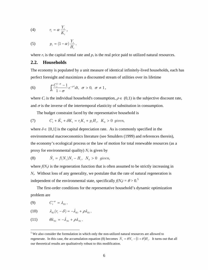
Dustin Chambers† and Jang-Ting Guo‡

September 3, 2007

∗ We are indebted to Shu-Hua Chen and Richard Suen for helpful discussions and comments. Part of this research was conducted while Guo was a visiting research fellow at the Institute of Economics, Academia Sinica, whose hospitality is greatly appreciated. Of course, all remaining errors are our own. † Department of Economics and Finance, Salisbury University, 1101 Camden Ave., Salisbury, MD 21801, 1-410-543-6320, Fax: 1-410-546-6208, E-mail: DLChambers@salisbury.edu. ‡ Corresponding Author. Department of Economics, 4128 Sproul Hall, University of California, Riverside, CA, 92521, 1-951-827-1588, Fax: 1-951-827-5685, E-mail: guojt@ucr.edu.

Abstract

This paper develops a one-sector endogenous growth model in which renewable natural

resources are postulated as both a factor of production and as a measure of environmental

quality. We show that sustained economic growth and a non-deteriorating environment

can coexist along the economy’s balanced growth path. Moreover, the output growth rate

is positively related to the steady-state level of natural-resource utilization in production.

Motivated by this theoretical prediction, we estimate a panel cross-country growth

regression model that includes a broad measure of productive natural resources – the

Ecological Footprint – as one of the conditioning variables, and find strong empirical

support. Our estimation results also suggest that the costs of environmental conservation

are fairly minimal, and that growth strategies based on greater physical capital formation

and openness to international trade outperform those relying on more intensive utilization

of the environment.

Keywords: Natural Resources; Endogenous Growth; Ecological Footprint. JEL Classification: O41; Q21; Q56.

1

1. Introduction In response to high energy prices and the OPEC oil embargo during the 1970’s,

economists began to systematically examine the growth effects of non-renewable natural

resources within dynamic general equilibrium macroeconomic models. For example,

using an exogenous-growth framework, Solow (1974) and Stiglitz (1974) show that

sustained economic growth is possible so long as the reproducible factor of production

(physical capital) can be substituted for exhaustible resources along the economy’s

balanced growth path.1 This finding, while unquestionably essential, is somewhat

restrictive in scope in that it ignores the impact of economic activities on the quality and

state of the environment. As a result, economists began to broaden their focus to

investigate the interrelations between economic growth and pollution emissions in the

1990’s. Specifically, Stokey (1998) finds that continuing growth is possible despite ever

tightening pollution restrictions that are met with costly abatement.2 More recently,

Brock and Taylor (2005) demonstrate the co-existence of sustained economic growth and

zero net pollution emissions (dubbed the “Kindergarten Rule”) in an endogenous growth

model in which the abatement technology improves through learning-by-doing.

Although this latter branch of the literature implicitly discusses the relationship between

economic development and environmental quality through the narrow lens of pollution, it

neglects the dual role that natural resources play in the production of GDP and hence

long-run economic growth. Motivated by this gap, we develop a one-sector endogenous

growth model that captures the environment’s roles as (i) a provider of factors of

production, and (ii) a stock of renewable natural resources that accumulates over time to

preserve environmental quality as GDP continues to grow. Our main finding is that in

the long run, the economy’s output growth rate is positively related to the steady-state

level of utilized natural resources. In addition, a panel cross-country growth regression,

which includes a broad measure of productive natural resources, provides strong

empirical support for this theoretical prediction.

1 Suzuki (1976) finds that continuing output growth can arise within environmental endogenous growth models as well. 2 See Lopez (1994) and Smulders and Gradus (1996) for other examples of growth models with pollution abatement.

2

The results of Solow (1974), Stiglitz (1974), and Stokey (1998), among others,

together suggest that sustained economic growth is possible despite limitations on the

productive availability of exhaustible natural resources, and that additional costs and

restrictions associated with preserving environmental quality are not an insurmountable

impediment to growth. By contrast, this paper focuses on the feasibility of a balanced-

growth-path equilibrium with non-deteriorating environmental quality in a canonical one-

sector endogenous growth model with renewable natural resources. In our model

economy, households live forever, provide fixed labor supply and derive utility from

consumption. A continuum of identical, competitive firms produce output using natural

resources, which are assumed to regenerate at a constant rate over time, as a factor of

production. The economy’s aggregate production function displays increasing returns-to-

scale because of the presence of productive externalities generated by capital inputs. We

show that along the balanced growth path (BGP), output, consumption, and physical

capital all grow at a common positive rate, whereas the stock of total natural resources

and the level of natural resources allocated to the firms’ production process maintain their

respective steady-state values.3 It follows that the quantity of utilized natural resources

per unit of GDP steadily declines in the economy’s BGP equilibrium, a result that is also

echoed in Solow (1974), Stiglitz (1974), and Stokey (1998) under non-renewable

resources. Furthermore, we find that an increase of natural-resource utilization in

production will raise the BGP’s output growth rate.

Next, to empirically verify our main theoretical finding, we incorporate an

inclusive measure of productive natural resources – the Ecological Footprint (EF) – into

Barro’s (1991) cross-country growth regression model. Formally, natural capital includes

all the productive resources that can be extracted from the earth, as well as all the

biological processes and services that facilitate life such as the absorption of waste or the

conversion of carbon-dioxide into oxygen. The EF series is based on this broader

concept of natural capital. As described in Rees (1992) and Wackernagel and Rees

(1996), the EF variable systematically measures the quantity of renewable natural

3 See Smulders (1999) for a survey of other mechanisms that also demonstrate the compatibility of continuing output growth and environmental preservation within the context of endogenous growth models.

3

resources and life-facilitating services demanded by each nation.4 In order to overcome

the inherent problem of aggregating over many disparate measures, the Ecological

Footprint is constructed by first converting an exhaustive and comprehensive list of

renewable natural resources and life-support services into standardized units of land area

called global hectares. The resulting quantity, expressed in per-capita terms, offers a

standardized measure of the land needed to support an average person’s consumption

expenditures (based on the country’s current level of per-capita income), and facilitate

ecologically necessary life-facilitating services. To our knowledge, the EF series is the

best available proxy for natural-resource utilization in the economy’s production process.

In addition to the Ecological Footprint, our dataset consists of a broad

international panel that includes 5-year growth spells of output, together with some

standard conditioning variables such as initial per-capita GDP, an educational attainment

proxy for human capital, government and investment’s shares of output, and trade

openness. In order to obtain unbiased estimates from our dynamic panel regressions,

Arellano and Bond’s (1991) two-step GMM estimation procedure is employed. We first

find that this empirical model passes the necessary specification tests whereby no second

or higher-order serial correlations in the estimation residuals are present. We then show

that the estimated coefficient on the Ecological Footprint is positive and statistically

significant at the 1% level. This estimation result provides strong empirical support for

the key prediction of our theoretical model, that is, more intensive utilization of natural

resources in production leads to an increase in the economy’s output growth rate.

Moreover, the signs and statistical significance of the remaining regressors are generally

in-line with neoclassical growth theory and previous empirical studies.

The remainder of this paper is organized as follows. Section 2 describes the

theoretical model and analyzes the equilibrium conditions for the economy’s balanced

growth path. Section 3 employs an international panel dataset that includes the

Ecological Footprint to empirically verify our main theoretical findings. Section 4

concludes.

4 The Ecological Footprint does not include measures of mineral deposits extracted in a given year.

4

2. The Theoretical Model We develop a one-sector environmental endogenous growth model in which the

representative household lives forever, provides fixed labor supply, and derives utility

from consumption. The economy’s social technology exhibits increasing returns-to-scale

because of the presence of productive externalities generated by capital inputs. For

analytical simplicity, and to maintain consistency with the subsequent empirical work

that employs the Ecological Footprint to measure environmental utilization, we assume

that all natural resources are renewable (such as a forest or fishery) in our theoretical

model. Moreover, some of the natural resources are used in the firm’s production

function to capture the environment’s productive value. Our analytical focus is to

explore the interrelations between the output growth rate and environmental quality along

the economy’s balanced growth path (BGP).

2.1. Firms There is a continuum of identical, competitive firms in the economy, with the total number

normalized to one. Each firm produces output Yt using a constant returns-to-scale Cobb-

Douglas production function

(1) , 10,1 <<= − αααtttt XHKY

where Kt and Ht are physical capital and harvested/utilized natural resources (or natural

capital), respectively, and Xt represents productive externalities that are taken as given by

individual firms. In addition, Xt is postulated to take the form

(2) ,0,1 >= − AKAX ttα

where tK denotes the economy-wide average level of the capital stock. In a symmetric

equilibrium, all firms take the same actions such that tt KK = . Hence, (2) can be substituted

into (1) to obtain the following social production function that displays increasing returns-to-

scale:

(3) . α−= 1ttt

HAKY

Under the assumption that factor markets are perfectly competitive, the first-order conditions

for the firm's profit maximization problem are given by

5

(4) t

tt K

Yr α= ,

(5) ,)1(t

tt H

Yp α−=

where rt is the capital rental rate and pt is the real price paid to utilized natural resources.

2.2. Households The economy is populated by a unit measure of identical infinitely-lived households, each has

perfect foresight and maximizes a discounted stream of utilities over its lifetime

(6) 1,0,1

10

1

≠>−− −∞ −

∫ σσσ

ρσ

dteC tt ,

where Ct is the individual household's consumption, ρ ∈ (0,1) is the subjective discount rate,

and σ is the inverse of the intertemporal elasticity of substitution in consumption.

The budget constraint faced by the representative household is

(7) ,0, 0 givenKHpKrKKC ttttttt >+=++ δ&

where δ ∈ [0,1] is the capital depreciation rate. As is commonly specified in the

environmental macroeconomics literature (see Smulders (1999) and references therein),

the economy’s ecological process or the law of motion for total renewable resources (as a

proxy for environmental quality) Nt is given by

(8) ,0,)( 0 givenNHNNfN tttt >−=&

where f(Nt) is the regeneration function that is often assumed to be strictly increasing in

Nt. Without loss of any generality, we postulate that the rate of natural regeneration is

independent of the environmental state, specifically f(Nt) = θ > 0.5

The first-order conditions for the representative household’s dynamic optimization

problem are

(9) , KttC λσ =−

(10) , KtKttKt r ρλλδλ +−=− &)(

(11) , NtNtNt ρλλθλ +−= &

5 We also consider the formulation in which only the non-utilized natural resources are allowed to regenerate. In this case, the accumulation equation (8) becomes ( ) .1 ttt HNN θθ +−=& It turns out that all our theoretical results are qualitatively robust to this modification.

6

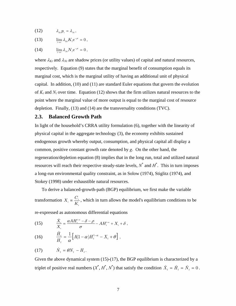
(12) NttKt

p λλ = ,

(13) 0=−

∞→

t

tKtteK ρλlim ,

(14) 0=−

∞→

t

tNtteN ρλlim ,

where λKt and λNt are shadow prices (or utility values) of capital and natural resources,

respectively. Equation (9) states that the marginal benefit of consumption equals its

marginal cost, which is the marginal utility of having an additional unit of physical

capital. In addition, (10) and (11) are standard Euler equations that govern the evolution

of Kt and Nt over time. Equation (12) shows that the firm utilizes natural resources to the

point where the marginal value of more output is equal to the marginal cost of resource

depletion. Finally, (13) and (14) are the transversality conditions (TVC).

2.3. Balanced Growth Path In light of the household’s CRRA utility formulation (6), together with the linearity of

physical capital in the aggregate technology (3), the economy exhibits sustained

endogenous growth whereby output, consumption, and physical capital all display a

common, positive constant growth rate denoted by g. On the other hand, the

regeneration/depletion equation (8) implies that in the long run, total and utilized natural

resources will reach their respective steady-state levels, N* and H*. This in turn imposes

a long-run environmental quality constraint, as in Solow (1974), Stiglitz (1974), and

Stokey (1998) under exhaustible natural resources.

To derive a balanced-growth-path (BGP) equilibrium, we first make the variable

transformation t

t

tK

CX ≡ , which in turn allows the model's equilibrium conditions to be

re-expressed as autonomous differential equations

(15) δσ

ρδα αα

++−−−

= −−

tt

t

t

t XAHAH

X

X 11&

,

(16) [ ]θαα

α +−−= −tt

t

t XHAHH 1)1(

1& ,

(17) . ttt HNN −= θ&

Given the above dynamical system (15)-(17), the BGP equilibrium is characterized by a

triplet of positive real numbers (X*, H*, N*) that satisfy the condition . 0=== ttt NHX &&&

7

It is straightforward to show that our model economy exhibits a unique balanced growth

path along which the utilized natural resource maintains its steady-state value

(18) )1/(1

*

)1(])1([

α

σαδσρσθ

−

⎥⎦

⎤⎢⎣

⎡−−−−

=A

H ,

which in turn leads to the expressions for X* and N* as follows:

(19) andθα α +−= −1** ))(1( HAXθ

** H

N = .

With (18) and (19), it follows that the common (positive) rate of economic growth g is

given by

(20) 1−

−=σ

ρθg or . ρθα α −−= −1*)(HAg

As a result, the BGP’s growth rate ceteris paribus is positively related to the level of

utilized natural resources.6 That is, a higher (lower) usage of services from the

environment in production will raise (reduce) the economy’s rate of growth in output,

consumption, and physical capital. Moreover, the quantity of utilized natural resources

per unit of GDP steadily declines along the economy’s balanced growth path, a result that

is also echoed in Solow (1974), Stiglitz (1974), and Stokey (1998), among many others.

3. The Empirical Model There are two interesting implications that follow from the above theoretical model.

First, as mentioned earlier, the BGP’s output growth rate rises with the productive

utilization of natural resources 0* >∂∂Hg . Second, the economy’s long-run rate of

economic growth increases with the reproduction rate of natural resources 0>∂∂θg . The

latter implication is difficult to verify empirically because of the need to access data on

the stock of natural resources, whereas the former is more easily testable given that it

requires the flow of natural resources used in production. As a result, we restrict our

empirical analysis to the effects of natural-resource utilization on GDP. Since output is a

6 To ensure that the BGP’s output growth rate g is positive, we impose the following parametric restriction: θ > (<) ρ when σ > (<) 1.

8

non-stationary variable, we cannot simply regress GDP on the aggregate factors of

production in levels. Instead, we incorporate the natural-resource usage into Barro’s

(1991) specification and examine the following panel cross-country growth regression

model:

(21) 1 1 2 3 4

5 6

growth income education gov inv trade footprint

it it it it it

it it i t it 1

β β ββ β α η ε

+

+

= + + ++ + + + +

β,

where the dependent variable ( 1growth it+ ) measures the average annual growth in real

GDP per capita in country i over the period of 5 years (between t and t+1). To account

for conditional convergence, our model includes , which is the natural log of

PPP-adjusted, chain-weighted per-capital GDP at period t. Human capital is controlled

by way of the proxy , which equals the average years of education for the

entire population aged 15 and above. To account for differences in fiscal policies across

countries, we include go , which measures public expenditures on goods and services

relative to GDP (= G

incomeit

education it

vit

it/Yit), as a conditioning variable. To control for the rate of capital

formation, the investment share in output (= Iit/Yit), denoted as , is also included.

The openness of a nation is captured by , which is the ratio of total trade to GDP,

that is (IM

invit

tradeit

it + EXit)/Yit. To control for the natural-resource utilization in production, we

include foot , which equals the natural log of the per-capita quantity of renewable

natural resources, in our panel estimation. Finally,

print it

iα is a country-specific effect, tη is a

period-specific effect, and 1itε + is an i.i.d. stochastic shock with zero mean and standard

deviation 2εσ .

3.1. The Data Our international panel dataset is constructed from three sources. Output growth,

income, government and investment’s shares of GDP, and trade openness are taken from

the Penn World Table v. 6.2 (Heston, Summers, and Aten, 2006). These variables are

expressed as percentages with the exception of income, which is expressed (prior to

taking the natural log) in constant (2000) international dollars ($I). The education series

comes from Barro and Lee (2000), and measures the average years of schooling for the

9

entire population aged 15 and above. Finally, the natural-resource series – the Ecological

Footprint – is obtained from the Global Footprint Network (2005).7 This variable

measures the quantity of renewable natural resources, in standardized global hectares

(gha), needed to produce a nation’s current level of per-capita consumption.8 In sum, our

dataset consists of an unbalanced panel of 93 countries over 9 five-year time periods

(1961, 1966, …, 2001), for a total of 794 observations. Table 1 lists the nations and

periods covered in the dataset, and Table 2 presents summary statistics of the raw,

untransformed data on the Ecological Footprint.

3.2. Estimation Method It is well known in the empirical growth literature that using standard fixed or random

effects methods to estimate a dynamic panel model such as (21) generates biased

estimates. Typically, this problem is resolved by use of a Generalized Method of

Moments (GMM) estimator along with suitable instruments. Within this family of

estimation procedures, Arellano and Bond’s (1991) 2-step estimator is one of the most

popular methods, and is also the estimator of choice for this paper. The first step of

Arellano and Bond’s estimation procedure is to take the first difference of (21), which,

after some algebraic manipulation, can be expressed as

(22) 1 1 2 3 4

5 6 1

income (1 ) income education gov inv trade footprint

it it it it it

it it t it

β β β ββ β η ε

+

+

∆ = + ∆ + ∆ + ∆ + ∆+ ∆ + ∆ + ∆ + ∆

,

thus the country-specific term iα is removed. The next step is to construct an appropriate

set of instruments. Generally speaking, the strictly exogenous variables in (22) can serve

as their own instruments, as well as lagged observations of the remaining predetermined,

untransformed endogenous variables. In the current context, we follow previous studies

(see, for example, Barro (2000) and Forbes (2000), among others) and postulate both the

series of income and investment’s share of output to be endogenous regressors.

7 See Haberl, Erb, and Krausmann (2001) for a good introduction on how ecological footprints are calculated. 8 Since this paper seeks to investigate how the rate of natural resource utilization affects economic growth, the total footprint series was adjusted by removing the per-capita quantity of developed land (i.e. urbanized space). The value of permanent improvements to land and the structures placed on land are generally included in a nation’s capital stock, thus including this area in a renewable resource (flow) measurement is inappropriate. The nuclear power component was removed from the footprint measure as well.

10

Moreover, since it is conceivable that a higher rate of economic growth boosts the

productive usage of the environment, we make the cautious modeling decision and treat

the natural-resource utilization as an endogenous conditioning variable as well. As a

result, our instrument set consists of all lagged values of income, investment’s share of

output, and ecological footprints, expressed in levels

{ }1 1 1 1 1income , , income ,inv , , inv , footprint , , footprintit i it i it i− − −K K K 1 , together with the

remaining (exogenous) regressors, expressed in differences

{ }education , gov , tradeit it it∆ ∆ ∆ , serving as their own instruments.9

3.3. Specification Tests Arellano and Bond (1991) state that the following two conditions must be satisfied for

their two-step GMM estimator to be consistent and efficient: (i) all of the regressors

(apart from the lagged dependent variable) must be predetermined by at least one period,

i.e. ( ) 0it isE X ε′ = for all , where s t> { }education ,gov ,inv , trade , footprintit it it it it itX ≡ in

this paper; and (ii) the model’s estimation errors cannot be autocorrelated, i.e.

( ) 0it isE ε ε = , for all . The first condition cannot be tested as a formal test does not

exist. However, Arellano and Bond (1991) propose two serial-correlation tests: the m

s t≠

2

test for second-order serial correlations, and the Sargan test for overidentifying

restrictions.10 Before reporting estimation results in the next subsection, we first conduct

these specification tests on our empirical model as in (22).

The m2 test for second-order autocorrelations in the residuals of (22) is crucially

important because lagged values of the right-hand side regressors are used as instruments

in the estimation procedure. Under the null hypothesis that there is no second-order

autocorrelation, the test statistic has an asymptotic standard normal distribution

(23) 2 *2 ~ (0,1)

am N

vε ε−′∆ ∆

= ,

9 The one exception is the time-period effects, which (as is customary) enter the instrument matrices in levels, not in differences. 10 As a third test, Arellano and Bond (1991) also suggest a Hausman specification test. However, using Monte Carlo experiments, these authors show that the Hausman test lacks power and is very susceptible to outliners. For this reason, Hausman specification tests are not commonly employed to test for serial correlation.

11

where 2ε−∆ is the vector of residuals from (22) lagged twice, *ε∆ is the vector of

residuals from the same model trimmed to match 2ε−∆ , and is a scalar that is defined

as

v

(24) ( )

1( 2) * * ( 2) 2 *

* ( 2) 2 * *

ˆ ˆ ˆ ˆ ˆ2 ( )

ˆˆ ˆ ˆ ˆ ˆ ˆ avar( )

i i i i N Ni N

i i i ii N

v X X Z

Z X

ε ε ε ε ε

2

A Z X X ZA

Xε ε ε ε δ ε

−− − −∈

− − −∈

′ ′ ′ ′ ′ ′≡ ∆ ∆ ∆ ∆ − ∆

′ ′ ′ ′× ∆ ∆ ∆ + ∆ ∆

∑∑

,

where X includes all the right-hand side conditioning variables, includes all the

estimated coefficients, Z is the matrix of instruments, and A

δ̂

N is the weighting matrix used

in the Arellano-Bond procedure. It turns out that for model (22), the m2 test statistic is

equal to 0.33, with a corresponding p-value of only 0.7415, yielding no evidence of

second-order autocorrelation.

As another check of our model’s estimation residuals, the Sargan test for

overidentifying restrictions is employed to confirm the validity of the moment restrictions

implied by the instruments. Under the null hypothesis that the moment restrictions are

valid (which implies the absence of second or higher-order autocorrelations), the test

statistic, denoted as s, is asymptotically chi-square distributed with q - k degrees of

freedom (i.e. 2q kχ − ):

(25) ( ) 12ˆ ˆ ˆ ˆ ~ i i i i qi N a

s Z Z Z Z kε ε ε ε χ−

−∈′′ ′ ′= ∆ ∆ ∆ ∆∑ ,

where q is the number of moment restrictions, and k is the number of coefficients

estimated in the model.

The Sargan test statistic for model (22) is equal to 82.86, with a corresponding p-

value of 0.44, hence we cannot reject the null hypothesis that the overidentifying

restrictions are valid. The above test results indicate that (22) lacks second or higher-

order serial correlations in the estimation residuals. Therefore, the two-step GMM

estimator that we report below is both consistent and efficient.

3.4. Estimation Results Before discussing our estimation results, it is instructive to examine the coefficient

estimates within a benchmark specification that excludes the footprint series from model

(22). Table 3 shows that the coefficient estimates from this standard formulation are

generally in-line with the existing empirical growth literature. In particular, the estimated

12

coefficient on initial income is negative and statistically significant at the 1% level,

indicating the presence of growth convergence, i.e. more developed nations ceteris

paribus grow more slowly than their less developed counterparts. The coefficients on

education, investment’s output share, and the degree of openness are all positive and

statistically significant. These results conform to the neoclassical growth theory where

increased accumulation in physical and human capital or higher volumes of international

trade will raise a nation’s output per worker. Finally, the estimated coefficient on

government expenditures is positive but marginally insignificant, with a p-value of 0.156.

Turing to a full estimate of model (22) with the footprint variable included, Table

3 shows that the estimated coefficients are very similar to those in the benchmark

specification.11 However, the coefficient on government’s share in GDP is now positive

and statistically significant, which is at odds with the findings of other researchers (see,

for example, Levine and Renelt (1992) and Barro (2000), among others). On the other

hand, consistent with the key prediction of our theoretical model, the estimated natural-

resource coefficient is positive and statistically significant at the 1% level. In other

words, when more natural resources (as measured in standardized global hectares) are

utilized in production within a nation, its subsequent 5-year growth rate in output will

rise.

Since the footprint series has been transformed by taking the natural log, the

estimated coefficient is interpreted as a growth elasticity measure. Specifically, a ten

percent increase in natural-resource utilization leads to a 0.17% rise in the annual growth

rate of GDP over the next 5-year period. Given the relatively small magnitude of this

effect, it would be inadvisable for an underdeveloped nation to rely too heavily on natural

resource extraction as a means of promoting economic growth. Instead, the estimation

results in Table 3 suggest that promoting domestic capital accumulation produces a much

larger quantitative impact on the economy’s future growth. In particular, a ten percent

increase in investment’s GDP share would boost the rate of output growth by almost

1.1%. Moreover, we note that a ten percent expansion in trade openness would enhance

11 Both the benchmark specification and model (22) include period dummies, whose estimated coefficients are not reported in Table 3. In addition, the Sargan test fails to reject the null hypothesis that the overidentifying restrictions are valid at any standard level of statistical significance in either formulation. See Table 3 for the respective test statistics and p-values.

13

economic growth by the same magnitude as the corresponding increase in natural-

resource usage. Therefore, our analysis offers some empirical support for adopting

mainstream growth strategies, such as promoting foreign direct investment and reaping

the gains from international trade, that are more economically rewarding and less harmful

to the environment. These results also suggests that developed nations should not be

overly opposed to well-reasoned conservation programs designed to slow down the rate

of natural-resource extraction because they appear to generate little drag on the economy.

In addition, anti-globalization efforts, i.e. opposition to the free flow of capital and goods

and services, will leave impoverished nations with few growth-promoting options.

Environmental degradation, be it for internal consumption (e.g. deforestation for small

homesteads) or external consumption (e.g. the export of raw commodities), is often the

result. This implies that anti-globalization, anti-poverty, and pro-environmental goals are

likely to be internally inconsistent.

4. Conclusion In examining long-run economic growth within the context of dynamic environmental

macroeconomic models, most of the existing literature has developed along the following

two strands: (i) the environment is a source of non-renewable factors of production, and

(ii) the state of the environment’s quality is measured by pollution emissions. In this

paper, we incorporate both of these environmental concerns, but from a different

perspective, into an otherwise standard one-sector endogenous growth model.

Specifically, the environment is postulated to be a storehouse of renewable natural

resources, some of which are used in the firm’s production process, that accumulate over

time to maintain environmental quality while output continues to grow. We show that

sustained economic growth and a non-deteriorating environment can be simultaneously

present along the economy’s balanced growth path. Moreover, we find that the BGP’s

output growth rate is positively related to the steady-state level of natural-resource

utilization in production.

To verify the empirical veracity of our theoretical findings, we estimate a panel

cross-country growth regression model that includes the Ecological Footprint, a broad

measure of productive natural resources, as one of the conditioning variables. The

14

estimation results provide strong empirical support for the positive relationship between

the utilization rate of natural resources in production and subsequent output growth.

However, this finding needs to be interpreted carefully since our empirical results also

suggest that the costs of environmental conservation are fairly minimal, and that growth

strategies based on greater physical capital formation and openness to trade outperform

those depending on more intensive use of the environment. In addition, it is important to

underscore that the BGP’ s output growth rate is positively related to the stationary, long-

run value of natural-resource utilization. Hence, higher usage of natural resources today

may boost economic growth in the short run, but will likely decrease its steady-state

level, thus permanently reducing the economy’s long-run rate of output growth. In light

of this short- vs. long-run growth tradeoff, and the fact that the short-run costs of

environmental conservation are relatively low, it is advisable that nations not rely heavily

on environmentally-intensive economic growth strategies.

15

References Arellano, M., and S. Bond (1991). “Some Tests of Specification for Panel Data: Monte

Carlo Evidence and an Application to Employment Equations,” Review of Economic Studies 58, 277-297.

Barro, R. J. (1991). “Economic Growth in a Cross-Section of Countries,” Quarterly

Journal of Economics 106, 407-444. Barro, R. J. (2000). “Inequality and Growth in a Panel of Countries,” Journal of

Economic Growth 5, 5-32. Barro, R. J., and J. Lee (2000). “International Data on Educational Attainment: Updates

and Implications,” Center for International Development, Harvard University, Working Paper No. 42. URL: http://www.cid.harvard.edu/ciddata/ciddata.html

Brock, W. A., and M. S. Taylor. (2005). “Economic Growth and the Environment: A

Review of Theory and Empirics,” in Handbook of Economic Growth, Vol. 1B, edited by. P. Aghion and S. N. Durlauf, Elsevier: Amsterdam, 1749-1821.

Forbes, K. (2000). “A Reassessment of the Relationship between Inequality and

Growth,” American Economic Review 90, 869-887. Global Footprint Network (2005). National Footprint and Biocapacity Accounts,

Academic Edition. URL: http://www.footprintnetwork.org Haberl, H., K. Erb and F. Krausmann (2001). “How to Calculate and Interpret Ecological

Footprints for Long Periods of Time: The Case of Austria 1926-1995,” Ecological Economics 38, 25-45.

Heston, A., R. Summers and B. Aten (2006). Penn World Table Version 6.2, Center for

International Comparisons of Production, Income and Prices, University of Pennsylvania. URL: http://pwt.econ.upenn.edu/

Levine, R., and D. Renelt (1992). “A Sensitivity Analysis of Cross-Country Growth

Regressions,” American Economic Review 82, 942-963. Lopez, R. (1994). “The Environment as a Factor of Production: The Effects of Economic

Growth and Trade Liberalization,” Journal of Environmental Economics and Management 27, 163-184.

Rees, W. (1992). “Ecological Footprints and Appropriated Carrying Capacity: What

Urban Economics Leaves Out,” Environment and Urbanization 4, 121-130. Smulders, S., and R. Gradus. (1996). “Pollution Abatement and Long-Term Growth,”

European Journal of Political Economy 12, 505-532.

16

Smulders, S. (1999). “Endogenous Growth Theory and the Environment,” in Handbook of Environmental and Resource Economics, edited by Jeroen C.J.M. van den Bergh, Edward Elgar: Cheltenham, UK, 610-621.

Solow, R. M. (1974). “Intergenerational Equity and Exhaustible Resources,” Review of

Economic Studies 41, 29-45. Stiglitz, J. (1974). “Growth with Exhaustible Natural Resources: Efficient and Optimal

Growth Paths,” Review of Economic Studies 41, 123-137. Stokey, N. L. (1998). “Are There Limits to Growth?” International Economic Review 39,

1-31. Suzuki, H. (1976). “On the Possibility of Steadily Growing Per Capita Consumption in an

Economy with a Wasting and Non-Replenishable Resource,” Review of Economic Studies 43, 527-535.

Wackernagel, M., and W. Rees (1996). Our Ecological Footprint, Reducing Human

Impact on the Earth, New Society Publishers: Philadelphia.

17

Table 1: Countries and Periods

Country Observations Range Country Observations RangeAfghanistan 7 1971-2001 Lesotho 9 1961-2001Algeria 9 1961-2001 Liberia 7 1971-2001Argentina 9 1961-2001 Malawi 9 1961-2001Australia 9 1961-2001 Malaysia 9 1961-2001Austria 9 1961-2001 Mali 9 1961-2001Bangladesh 6 1976-2001 Mauritius 9 1961-2001Benin 9 1961-2001 Mexico 9 1961-2001Bolivia 9 1961-2001 Mozambique 9 1961-2001Botswana 7 1971-2001 Nepal 9 1961-2001Brazil 9 1961-2001 Netherlands 9 1961-2001Cameroon 9 1961-2001 New Zealand 9 1961-2001Canada 9 1961-2001 Nicaragua 9 1961-2001Central African Republic 7 1971-2001 Niger 9 1961-2001Chile 9 1961-2001 Norway 9 1961-2001China 6 1976-2001 Pakistan 9 1961-2001Colombia 9 1961-2001 Panama 9 1961-2001Congo, Republic of 4 1986-2001 Papua New Guinea 7 1971-2001Costa Rica 9 1961-2001 Paraguay 9 1961-2001Denmark 9 1961-2001 Peru 9 1961-2001Dominican Republic 9 1961-2001 Philippines 9 1961-2001Ecuador 9 1961-2001 Poland 7 1971-2001Egypt 6 1976-2001 Portugal 9 1961-2001El Salvador 9 1961-2001 Rwanda 9 1961-2001Finland 9 1961-2001 Senegal 9 1961-2001France 9 1961-2001 Sierra Leone 7 1971-2001Gambia, The 9 1961-2001 South Africa 9 1961-2001Germany 7 1971-2001 Spain 9 1961-2001Ghana 9 1961-2001 Sri Lanka 9 1961-2001Greece 9 1961-2001 Sudan 7 1971-2001Guatemala 9 1961-2001 Swaziland 7 1971-2001Guinea-Bissau 9 1961-2001 Sweden 9 1961-2001Haiti 6 1971-1996 Switzerland 9 1961-2001Honduras 9 1961-2001 Syria 9 1961-2001Hungary 7 1971-2001 Tanzania 9 1961-2001India 9 1961-2001 Thailand 9 1961-2001Indonesia 9 1961-2001 Togo 9 1961-2001Iran 9 1961-2001 Trinidad &Tobago 9 1961-2001Iraq 7 1971-2001 Tunisia 9 1961-2001Ireland 9 1961-2001 Turkey 9 1961-2001Israel 9 1961-2001 Uganda 9 1961-2001Italy 9 1961-2001 United Kingdom 9 1961-2001Jamaica 9 1961-2001 United States 9 1961-2001Japan 9 1961-2001 Uruguay 9 1961-2001Jordan 9 1961-2001 Venezuela 9 1961-2001Kenya 9 1961-2001 Zambia 9 1961-2001Korea, Republic of 9 1961-2001 Zimbabwe 9 1961-2001Kuwait 7 1971-2001

18

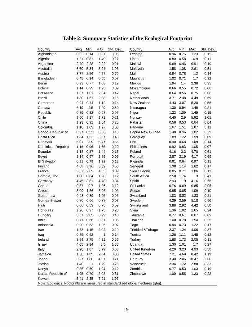
Country Avg Min Max Std. Dev. Country Avg Min Max Std. Dev.Afghanistan 0.22 0.14 0.31 0.06 Lesotho 0.96 0.75 1.23 0.15Algeria 1.21 0.81 1.49 0.27 Liberia 0.80 0.58 0.9 0.11Argentina 2.70 2.28 2.92 0.21 Malawi 0.69 0.46 0.91 0.19Australia 6.60 5.34 8.24 1.06 Malaysia 1.58 1.08 2.61 0.51Austria 3.77 2.56 4.67 0.70 Mali 0.94 0.78 1.2 0.14Bangladesh 0.45 0.34 0.55 0.07 Mauritius 1.02 0.71 1.7 0.32Benin 0.93 0.77 1.08 0.12 Mexico 1.94 1.4 2.38 0.35Bolivia 1.14 0.99 1.25 0.09 Mozambique 0.66 0.55 0.72 0.06Botswana 1.37 1.01 2.34 0.47 Nepal 0.64 0.56 0.75 0.06Brazil 1.80 1.61 2.08 0.15 Netherlands 3.71 2.48 4.49 0.69Cameroon 0.94 0.74 1.12 0.14 New Zealand 4.43 3.87 5.38 0.56Canada 6.19 4.5 7.29 0.80 Nicaragua 1.30 0.94 1.49 0.21Republic 0.89 0.82 0.98 0.07 Niger 1.32 1.09 1.49 0.15Chile 1.50 1.17 1.71 0.21 Norway 4.40 2.9 5.92 1.01China 1.23 0.91 1.54 0.25 Pakistan 0.58 0.53 0.64 0.04Colombia 1.16 1.09 1.27 0.06 Panama 1.67 1.51 1.87 0.11Congo, Republic of 0.67 0.52 0.86 0.16 Papua New Guinea 1.48 0.96 1.82 0.29Costa Rica 1.84 1.53 3.07 0.48 Paraguay 1.89 1.72 1.99 0.09Denmark 5.01 3.9 6.77 0.85 Peru 0.90 0.68 1.09 0.14Dominican Republic 1.16 0.96 1.65 0.20 Philippines 0.92 0.83 1.05 0.07Ecuador 1.18 0.87 1.44 0.16 Poland 4.16 3.3 4.78 0.61Egypt 1.14 0.97 1.25 0.09 Portugal 2.87 2.19 4.17 0.69El Salvador 0.91 0.79 1.22 0.13 Rwanda 0.81 0.64 0.97 0.11Finland 4.68 3.96 5.52 0.50 Senegal 1.38 1.14 1.62 0.17France 3.67 2.89 4.05 0.39 Sierra Leone 0.85 0.71 1.06 0.13Gambia, The 1.08 0.84 1.28 0.12 South Africa 2.50 1.74 3 0.41Germany 4.45 3.81 4.78 0.34 Spain 2.93 1.9 4.16 0.66Ghana 0.87 0.7 1.06 0.12 Sri Lanka 0.76 0.69 0.85 0.05Greece 3.09 1.86 5.06 1.03 Sudan 0.95 0.85 1.09 0.10Guatemala 0.93 0.89 1.05 0.05 Swaziland 1.03 0.82 1.33 0.21Guinea-Bissau 0.80 0.66 0.88 0.07 Sweden 4.29 3.59 5.18 0.56Haiti 0.66 0.53 0.75 0.09 Switzerland 3.88 2.92 4.42 0.50Honduras 1.26 0.97 1.75 0.26 Syria 1.36 1.02 1.65 0.24Hungary 3.57 2.85 3.99 0.46 Tanzania 0.77 0.61 0.87 0.09India 0.71 0.66 0.81 0.05 Thailand 1.00 0.78 1.54 0.25Indonesia 0.90 0.83 1.05 0.07 Togo 0.94 0.73 1.22 0.17Iran 1.53 1.15 2.02 0.29 Trinidad &Tobago 2.37 1.24 4.06 0.87Iraq 0.85 0.62 1 0.14 Tunisia 1.26 1.11 1.45 0.12Ireland 3.84 2.75 4.91 0.65 Turkey 1.88 1.73 2.05 0.11Israel 4.05 2.34 8.5 1.83 Uganda 1.30 1.01 1.7 0.27Italy 2.98 1.87 3.79 0.63 United Kingdom 4.29 3.23 4.93 0.50Jamaica 1.56 1.09 2.04 0.33 United States 7.21 4.69 8.42 1.19Japan 3.27 1.88 4.07 0.71 Uruguay 3.40 2.06 10.47 2.66Jordan 1.40 1 1.79 0.26 Venezuela 2.34 1.72 2.88 0.33Kenya 0.86 0.69 1.04 0.12 Zambia 0.77 0.53 1.03 0.19Korea, Republic of 1.95 0.79 3.08 0.81 Zimbabwe 1.00 0.55 1.23 0.22Kuwait 5.41 2.35 7.91 1.97Note: Ecological Footprints are measured in standardized global hectares (gha).

Table 2: Summary Statistics of the Ecological Footprint

19

Table 3: Two-Step GMM Estimation Results

Variable Benchmark Model (22)income -0.0493 -0.064

(0.0012)*** (0.0010)***education 0.0099 0.013

(0.0025)*** (0.0011)***government 0.0241 0.057

(0.0170) (0.0080)***investment 0.1054 0.106

(0.0241)*** (0.0122)***trade 0.0174 0.017

(0.0063)*** (0.0033)***footprint 0.017

(0.0027)***

Sargan test 64.44 82.86Sargan p-value 0.156 0.422

Observations 608 608White robust (period) standard errors in parenthesis***,**,** - statistically significant at the one, five, and ten percent levels respectively

20