A New Cyberinfrastructure for the Natural Hazards Community

1

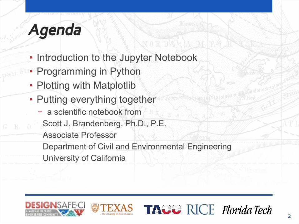
Agenda

• Introduction to the Jupyter Notebook• Programming in Python• Plotting with Matplotlib• Putting everything together

− a scientific notebook from Scott J. Brandenberg, Ph.D., P.E.Associate ProfessorDepartment of Civil and Environmental EngineeringUniversity of California

2

What are Jupyter Notebooks?

A web-based, interactive computing tool for capturing the whole computation process: developing, documenting, and executing code, as well as communicating the results.

3

How do Jupyter Notebooks Work?

An open notebook has exactly one interactive session connected to a kernel which will execute code sent by the user and communicate back results. This kernel remains active if the web browser window is closed, and reopening the same notebook from the dashboard will reconnect the web application to the same kernel.

What's this mean?Notebooks are an interface to kernel, the kernel executes your code and outputs back to you through the notebook. The kernel is essentially our programming language we wish to interface with.

4

Jupyter Notebooks, Structure

• Code Cells− Code cells allow you to enter and run code

Run a code cell using Shift-Enter

• Markdown Cells− Text can be added to Jupyter Notebooks using Markdown

cells. Markdown is a popular markup language that is a superset of HTML.

5

Jupyter Notebooks, Structure

• Markdown Cells− You can add headings:

• # Heading 1

# Heading 2

## Heading 2.1## Heading 2.2

− You can add lists• 1. First ordered list item

2. Another item

⋅⋅* Unordered sub-list.

1. Actual numbers don't matter, just that it's a number

⋅⋅1. Ordered sub-list4. And another item.

6

Jupyter Notebooks, Structure

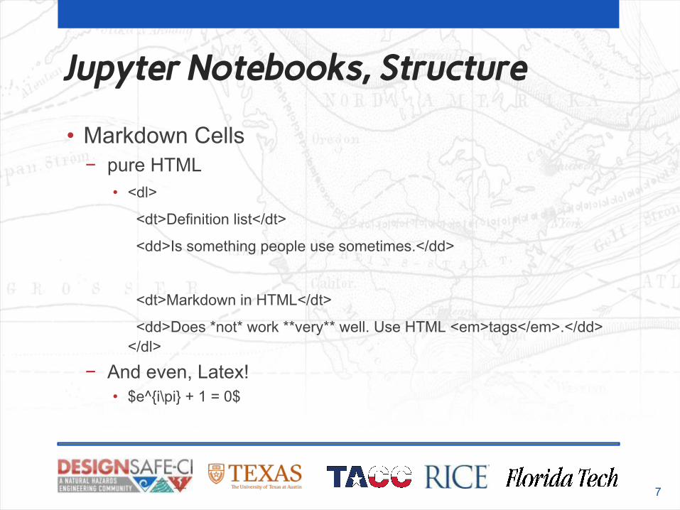
• Markdown Cells− pure HTML

• <dl>

<dt>Definition list</dt>

<dd>Is something people use sometimes.</dd>

<dt>Markdown in HTML</dt>

<dd>Does *not* work **very** well. Use HTML <em>tags</em>.</dd></dl>

− And even, Latex!• $e^{i\pi} + 1 = 0$

7

Jupyter Notebooks, Workflow

Typically, you will work on a computational problem in pieces, organizing related ideas into cells and moving forward once previous parts work correctly. This is much more convenient for interactive exploration than breaking up a computation into scripts that must be executed together, as was previously necessary, especially if parts of them take a long time to run.

8

Jupyter Notebooks, Workflow

• Let a traditional paper lab notebook be your guide:

− Each notebook keeps a historical (and dated) record of the analysis as it’s being explored.

− The notebook is not meant to be anything other than a place for experimentation and development.

− Notebooks can be split when they get too long.

− Notebooks can be split by topic, if it makes sense.

9

Jupyter Notebooks, Shortcuts

● Shift-Enter: run cell

● Execute the current cell, show output (if any), and jump to the

next cell below. If Shift-Enteris invoked on the last cell, a

new code cell will also be created. Note that in the notebook,

typing Enter on its own never forces execution, but rather just

inserts a new line in the current cell. Shift-Enter is equivalent

to clicking the Cell | Run menu item.

10

Jupyter Notebooks, Shortcuts

● Ctrl-Enter: run cell in-place

● Execute the current cell as if it were in “terminal mode”, where

any output is shown, but the cursor remains in the current cell.

The cell’s entire contents are selected after execution, so you

can just start typing and only the new input will be in the cell.

This is convenient for doing quick experiments in place, or for

querying things like filesystem content, without needing to

create additional cells that you may not want to be saved in the

notebook.

11

Jupyter Notebooks, Shortcuts

● Alt-Enter: run cell, insert below

● Executes the current cell, shows the output, and inserts a new

cell between the current cell and the cell below (if one exists).

(shortcut for the sequence Shift-Enter,Ctrl-m a. (Ctrl-m a

adds a new cell above the current one.))

● Esc and Enter: Command mode and edit mode

● In command mode, you can easily navigate around the

notebook using keyboard shortcuts. In edit mode, you can edit

text in cells.

12

Introduction to Python

• Hello World!• Data types• Variables• Arithmetic operations• Relational operations• Input/Output• Control Flow• More Data Types!• Matplotlib

13

the magic number is:

4

Python

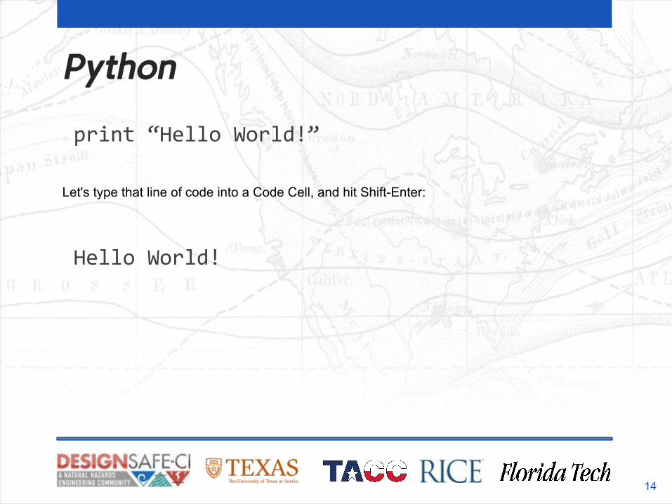
print “Hello World!”

14

Let's type that line of code into a Code Cell, and hit Shift-Enter:

Hello World!

Python

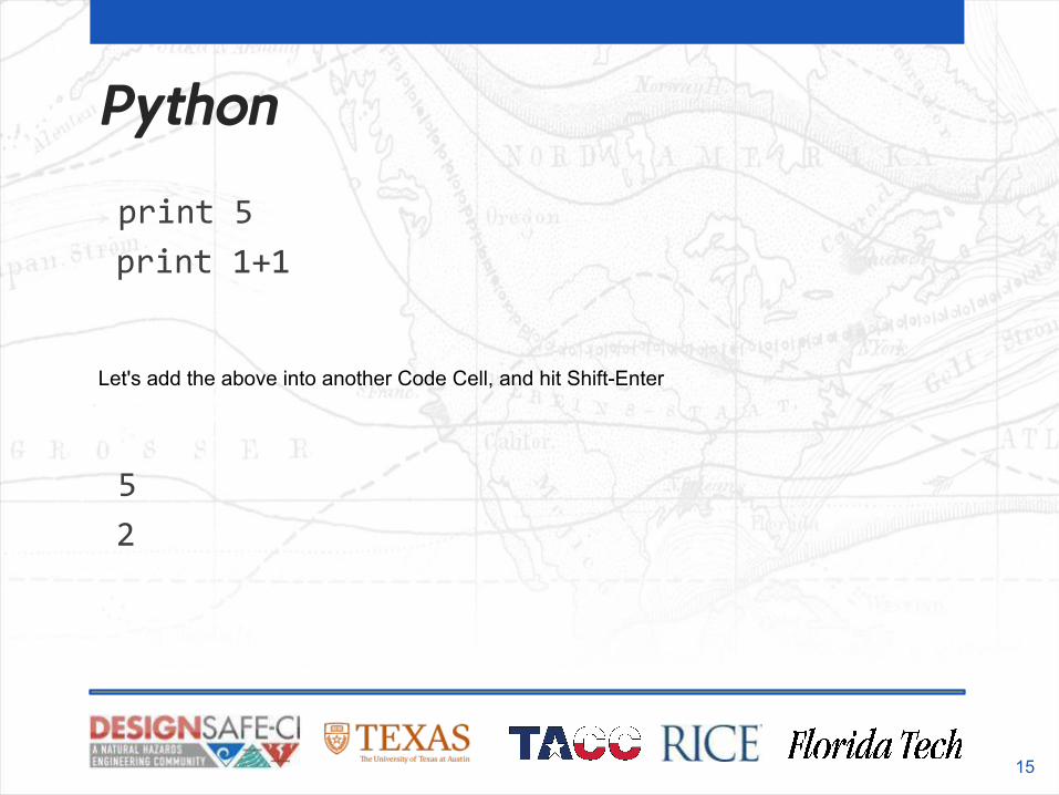
print 5

print 1+1

15

Let's add the above into another Code Cell, and hit Shift-Enter

5

2

Python - Variables

16

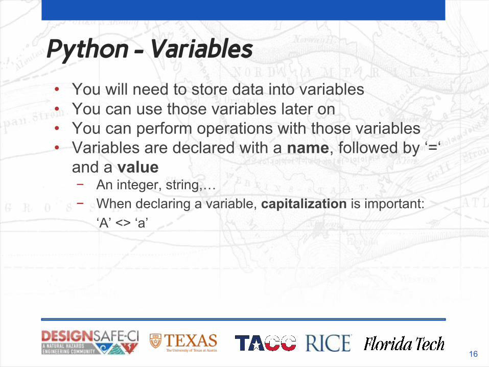
• You will need to store data into variables• You can use those variables later on• You can perform operations with those variables• Variables are declared with a name, followed by ‘=‘

and a value− An integer, string,…− When declaring a variable, capitalization is important:

‘A’ <> ‘a’

Python - Variables

17

in a code cell:

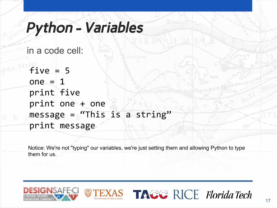
five = 5one = 1print fiveprint one + onemessage = “This is a string”print message

Notice: We're not "typing" our variables, we're just setting them and allowing Python to type them for us.

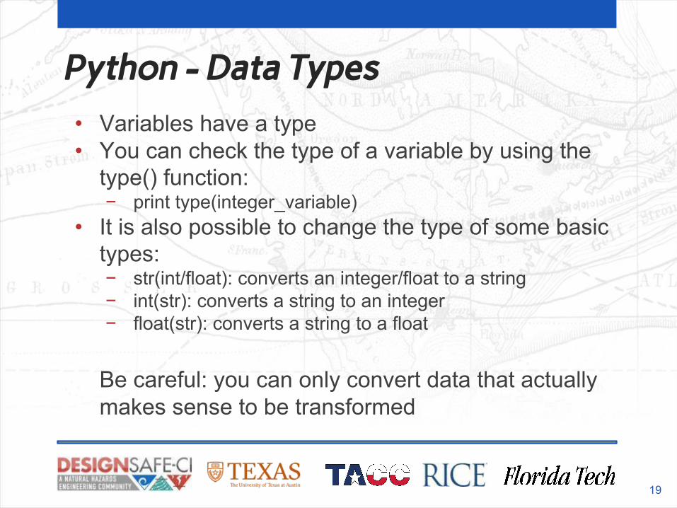
Python - Data Types

18

in a code cell:

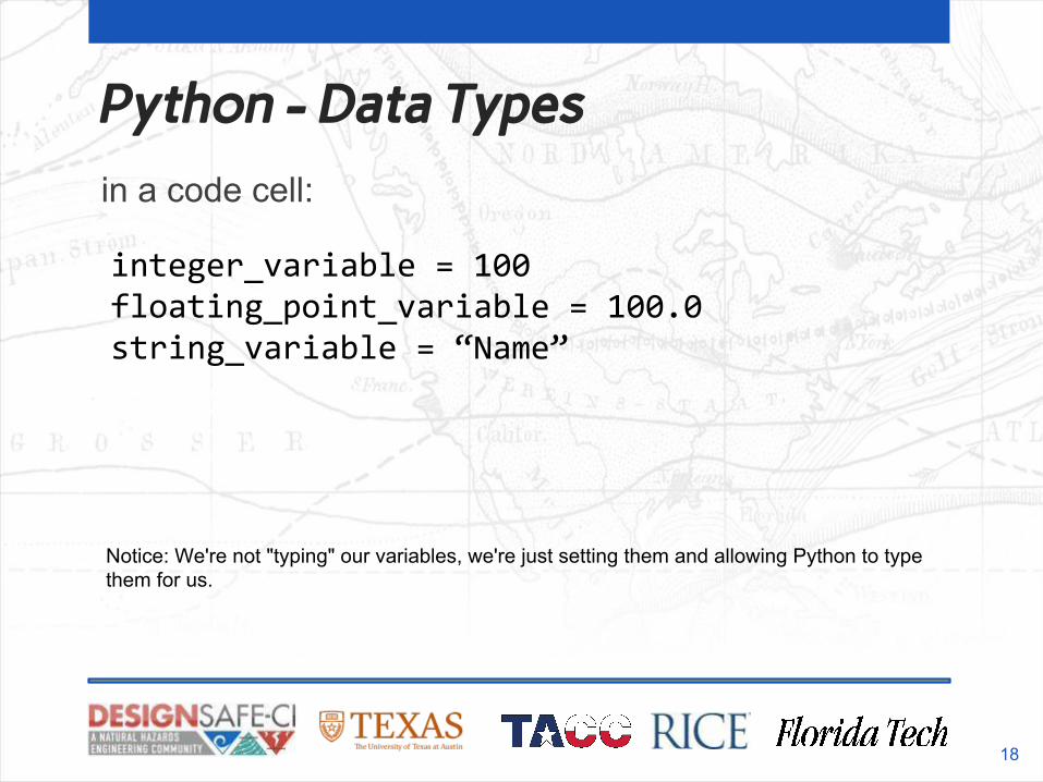
integer_variable = 100floating_point_variable = 100.0string_variable = “Name”

Notice: We're not "typing" our variables, we're just setting them and allowing Python to type them for us.

Python - Data Types

19

• Variables have a type• You can check the type of a variable by using the

type() function:− print type(integer_variable)

• It is also possible to change the type of some basic types:− str(int/float): converts an integer/float to a string− int(str): converts a string to an integer− float(str): converts a string to a float

Be careful: you can only convert data that actually makes sense to be transformed

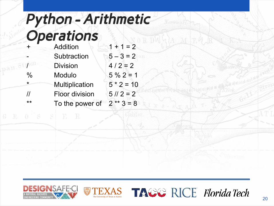
Python - Arithmetic Operations

20

+ Addition 1 + 1 = 2- Subtraction 5 – 3 = 2/ Division 4 / 2 = 2% Modulo 5 % 2 = 1* Multiplication 5 * 2 = 10// Floor division 5 // 2 = 2** To the power of 2 ** 3 = 8

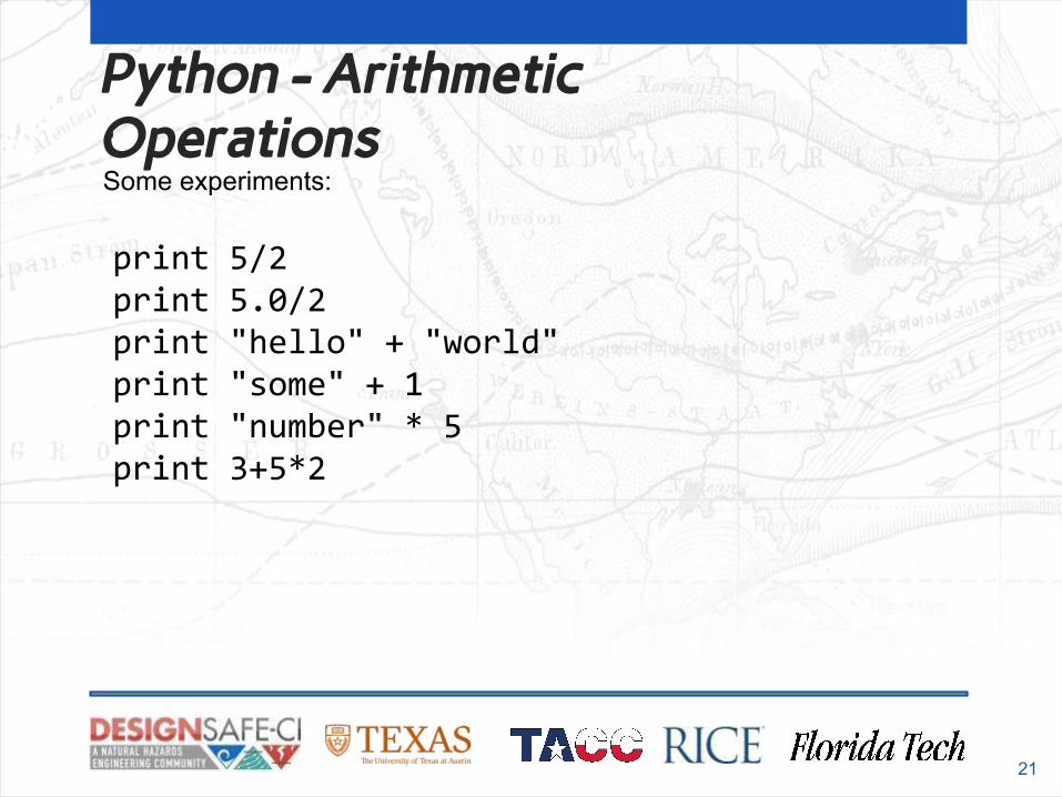
Python - Arithmetic Operations

21

Some experiments:

print 5/2print 5.0/2print "hello" + "world"print "some" + 1print "number" * 5print 3+5*2

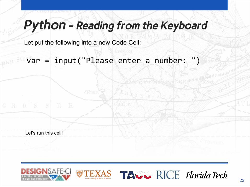
Python - Reading from the Keyboard

22

Let put the following into a new Code Cell:

var = input("Please enter a number: ")

Let's run this cell!

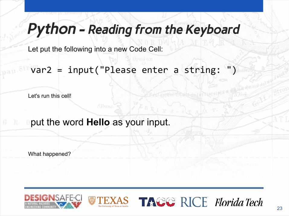
Python - Reading from the Keyboard

23

Let put the following into a new Code Cell:

var2 = input("Please enter a string: ")

Let's run this cell!

put the word Hello as your input.

What happened?

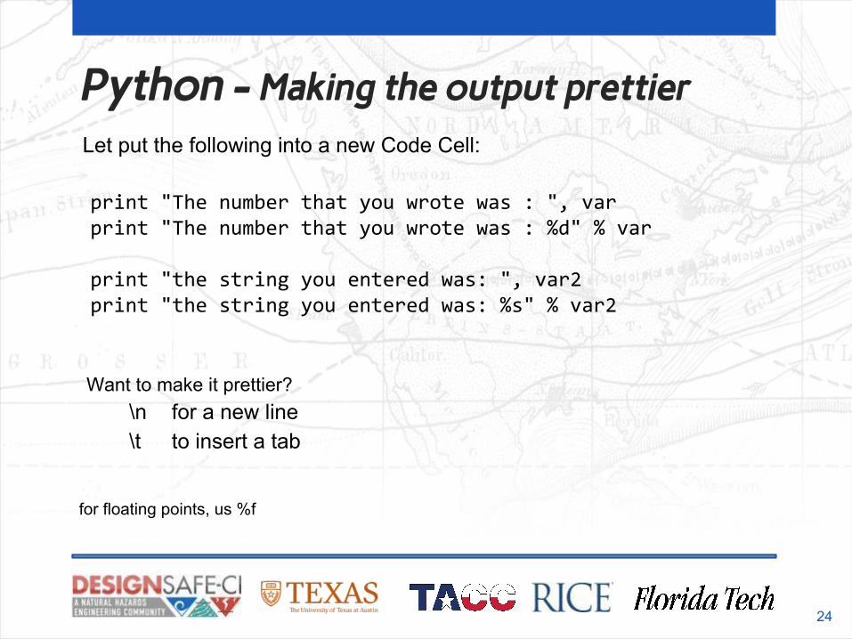
Python - Making the output prettier

24

Let put the following into a new Code Cell:

print "The number that you wrote was : ", varprint "The number that you wrote was : %d" % var

print "the string you entered was: ", var2print "the string you entered was: %s" % var2

for floating points, us %f

Want to make it prettier?\n for a new line\t to insert a tab

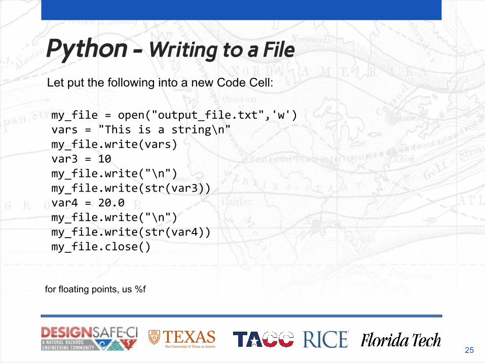
Python - Writing to a File

25

Let put the following into a new Code Cell:

my_file = open("output_file.txt",'w')vars = "This is a string\n"my_file.write(vars)var3 = 10my_file.write("\n")my_file.write(str(var3))var4 = 20.0my_file.write("\n")my_file.write(str(var4))my_file.close()

for floating points, us %f

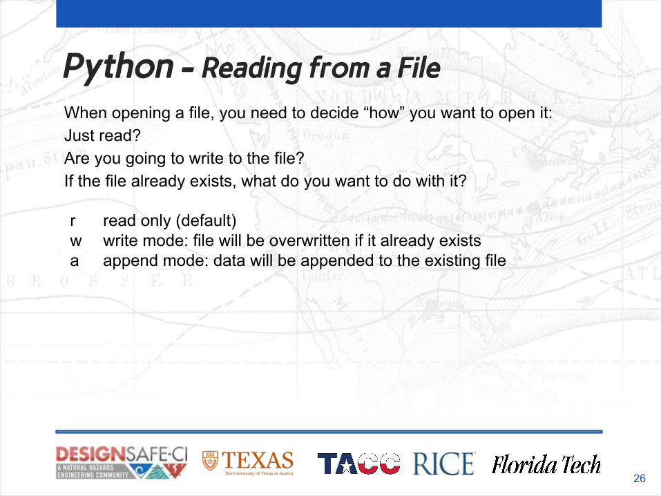
Python - Reading from a File

26

When opening a file, you need to decide “how” you want to open it:Just read?Are you going to write to the file?If the file already exists, what do you want to do with it?

r read only (default)w write mode: file will be overwritten if it already existsa append mode: data will be appended to the existing file

Python - Reading from a File

27

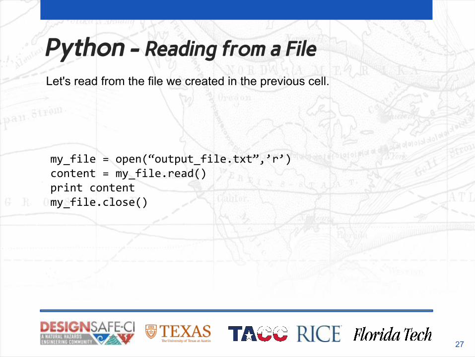
Let's read from the file we created in the previous cell.

my_file = open(“output_file.txt”,’r’)content = my_file.read()print contentmy_file.close()

Python - Reading from a File

28

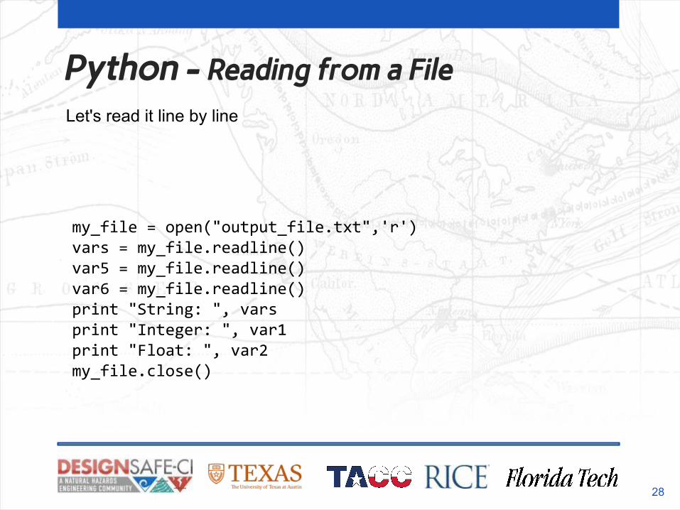
Let's read it line by line

my_file = open("output_file.txt",'r')vars = my_file.readline()var5 = my_file.readline()var6 = my_file.readline()print "String: ", varsprint "Integer: ", var1print "Float: ", var2my_file.close()

Python - Reading from a File

29

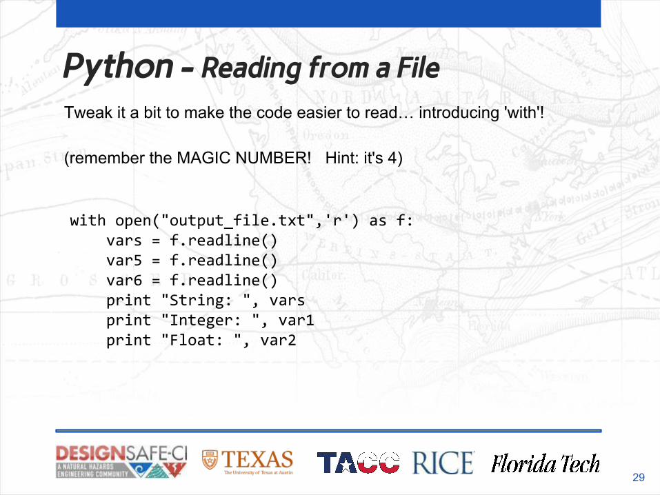
Tweak it a bit to make the code easier to read… introducing 'with'!

(remember the MAGIC NUMBER! Hint: it's 4)

with open("output_file.txt",'r') as f: vars = f.readline() var5 = f.readline() var6 = f.readline() print "String: ", vars print "Integer: ", var1 print "Float: ", var2

Python - Control Flow

30

• So far we have been writing instruction after instruction• Every instruction is executed• What happens if we want to have instructions that are only executed

if a given condition is true?

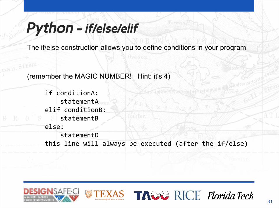
Python - if/else/elif

31

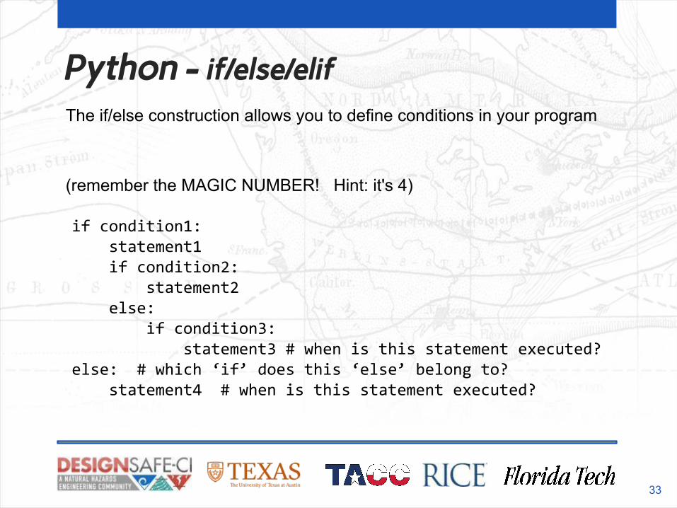
The if/else construction allows you to define conditions in your program

(remember the MAGIC NUMBER! Hint: it's 4)

if conditionA: statementA elif conditionB: statementB else: statementD this line will always be executed (after the if/else)

Python - if/else/elif

32

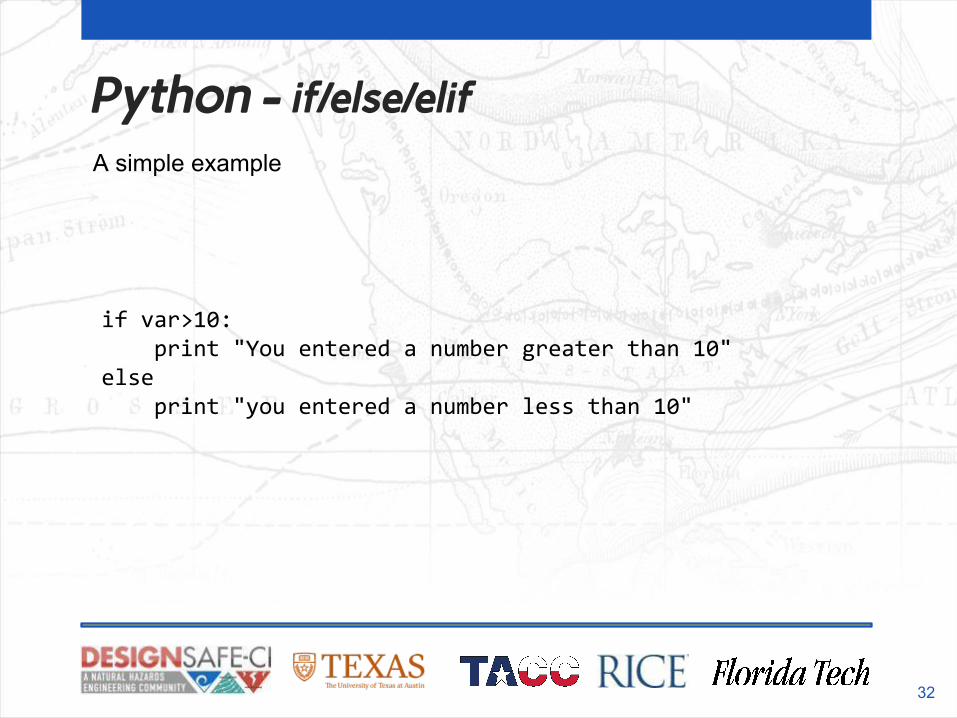
A simple example

if var>10: print "You entered a number greater than 10"else print "you entered a number less than 10"

Python - if/else/elif

33

The if/else construction allows you to define conditions in your program

(remember the MAGIC NUMBER! Hint: it's 4)

if condition1: statement1 if condition2: statement2 else: if condition3: statement3 # when is this statement executed?else: # which ‘if’ does this ‘else’ belong to? statement4 # when is this statement executed?

Python - For Loops

34

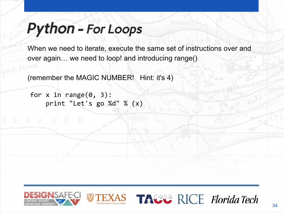
When we need to iterate, execute the same set of instructions over and over again… we need to loop! and introducing range()

(remember the MAGIC NUMBER! Hint: it's 4)

for x in range(0, 3): print "Let's go %d" % (x)

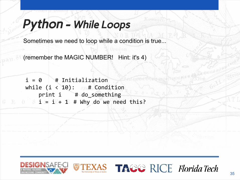
Python - While Loops

35

Sometimes we need to loop while a condition is true...

(remember the MAGIC NUMBER! Hint: it's 4)

i = 0 # Initializationwhile (i < 10): # Condition print i # do_something i = i + 1 # Why do we need this?

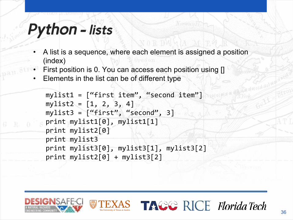
Python - lists

36

• A list is a sequence, where each element is assigned a position (index)

• First position is 0. You can access each position using []• Elements in the list can be of different type

mylist1 = [“first item”, “second item”]mylist2 = [1, 2, 3, 4]mylist3 = [“first”, “second”, 3]print mylist1[0], mylist1[1]print mylist2[0]print mylist3print mylist3[0], mylist3[1], mylist3[2]print mylist2[0] + mylist3[2]

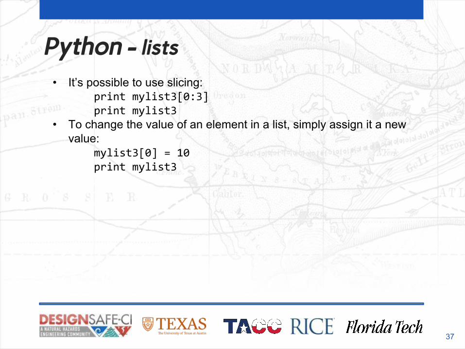
Python - lists

37

• It’s possible to use slicing: print mylist3[0:3] print mylist3

• To change the value of an element in a list, simply assign it a new value: mylist3[0] = 10 print mylist3

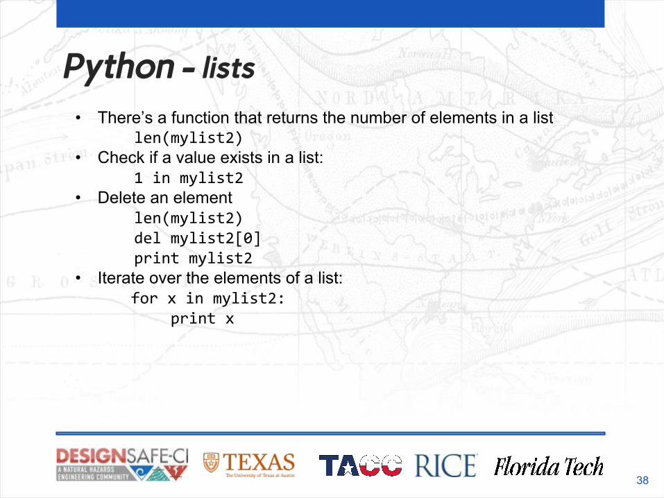
Python - lists

38

• There’s a function that returns the number of elements in a list len(mylist2)

• Check if a value exists in a list: 1 in mylist2

• Delete an element len(mylist2) del mylist2[0] print mylist2

• Iterate over the elements of a list: for x in mylist2: print x

Python - lists

39

• There are more functions max(mylist), min(mylist)

• It’s possible to add new elements to a list: my_list.append(new_item)

• We know how to find if an element exists, but there’s a way to return the position of that element: my_list.index(item)

• Or how many times a given item appears in the list: my_list.count(item)

Matplotlib, What is it?

It’s a graphing library for Python. It has a nice collection of tools that you can use to create anything from simple graphs, to scatter plots, to 3D graphs. It is used heavily in the scientific Python community for data visualisation.

40

Matplotlib, First Steps

Let's plot a simple sin wave from 0 to 2 pi.First lets, get our code started by importing the necessary modules.

41

%matplotlib inline

import matplotlib.pyplot as plt

import numpy as np

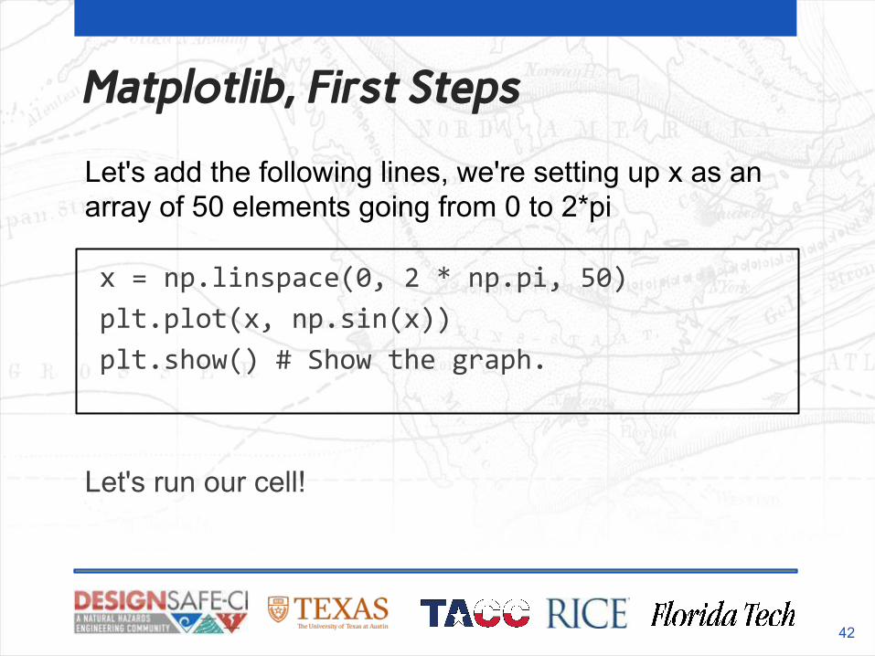
Matplotlib, First Steps

x = np.linspace(0, 2 * np.pi, 50)

plt.plot(x, np.sin(x))

plt.show() # Show the graph.

Let's run our cell!

42

Let's add the following lines, we're setting up x as an array of 50 elements going from 0 to 2*pi

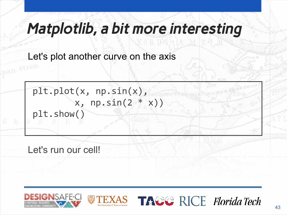
Matplotlib, a bit more interesting

plt.plot(x, np.sin(x), x, np.sin(2 * x))plt.show()

Let's run our cell!

43

Let's plot another curve on the axis

Matplotlib, a bit more interesting

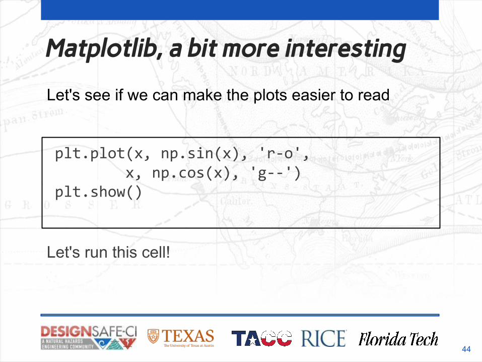
plt.plot(x, np.sin(x), 'r-o', x, np.cos(x), 'g--')plt.show()

Let's run this cell!

44

Let's see if we can make the plots easier to read

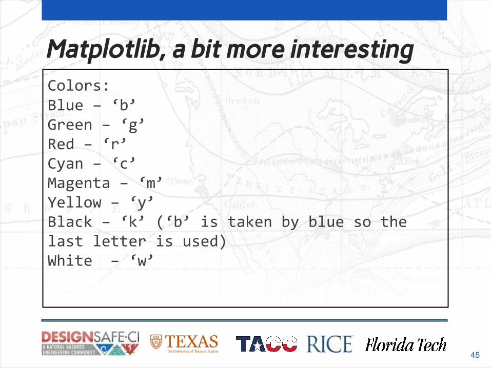
Matplotlib, a bit more interestingColors:Blue – ‘b’Green – ‘g’Red – ‘r’Cyan – ‘c’Magenta – ‘m’Yellow – ‘y’Black – ‘k’ (‘b’ is taken by blue so the last letter is used)White – ‘w’

45

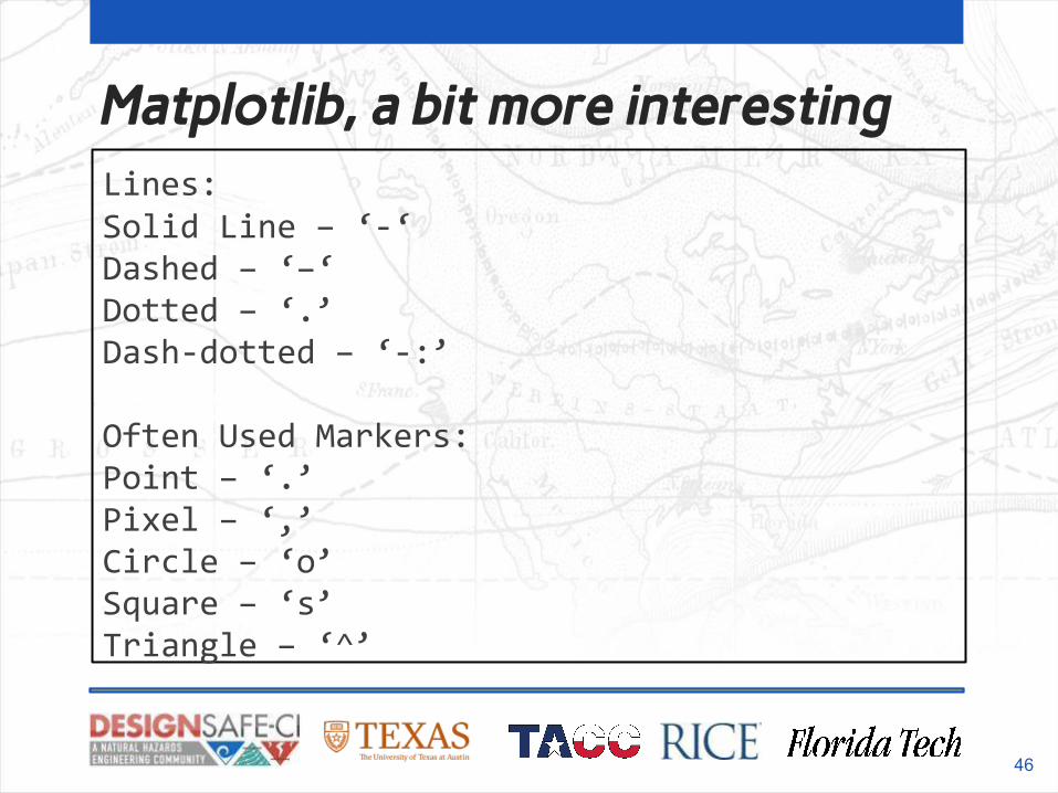
Matplotlib, a bit more interestingLines:Solid Line – ‘-‘Dashed – ‘–‘Dotted – ‘.’Dash-dotted – ‘-:’

Often Used Markers:Point – ‘.’Pixel – ‘,’Circle – ‘o’Square – ‘s’Triangle – ‘^’

46

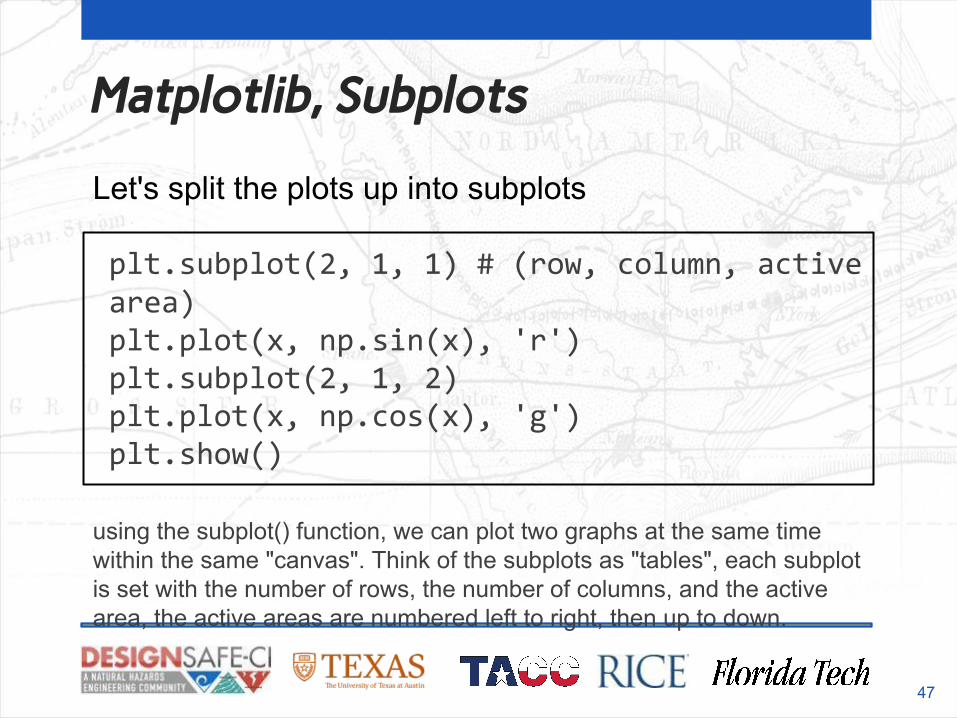
Matplotlib, Subplots

plt.subplot(2, 1, 1) # (row, column, active area)plt.plot(x, np.sin(x), 'r')plt.subplot(2, 1, 2)plt.plot(x, np.cos(x), 'g')plt.show()

using the subplot() function, we can plot two graphs at the same time within the same "canvas". Think of the subplots as "tables", each subplot is set with the number of rows, the number of columns, and the active area, the active areas are numbered left to right, then up to down.

47

Let's split the plots up into subplots

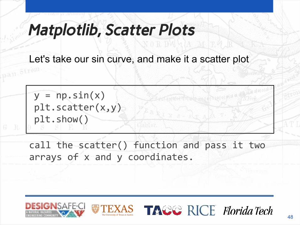
Matplotlib, Scatter Plots

y = np.sin(x)plt.scatter(x,y)plt.show()

call the scatter() function and pass it two arrays of x and y coordinates.

48

Let's take our sin curve, and make it a scatter plot

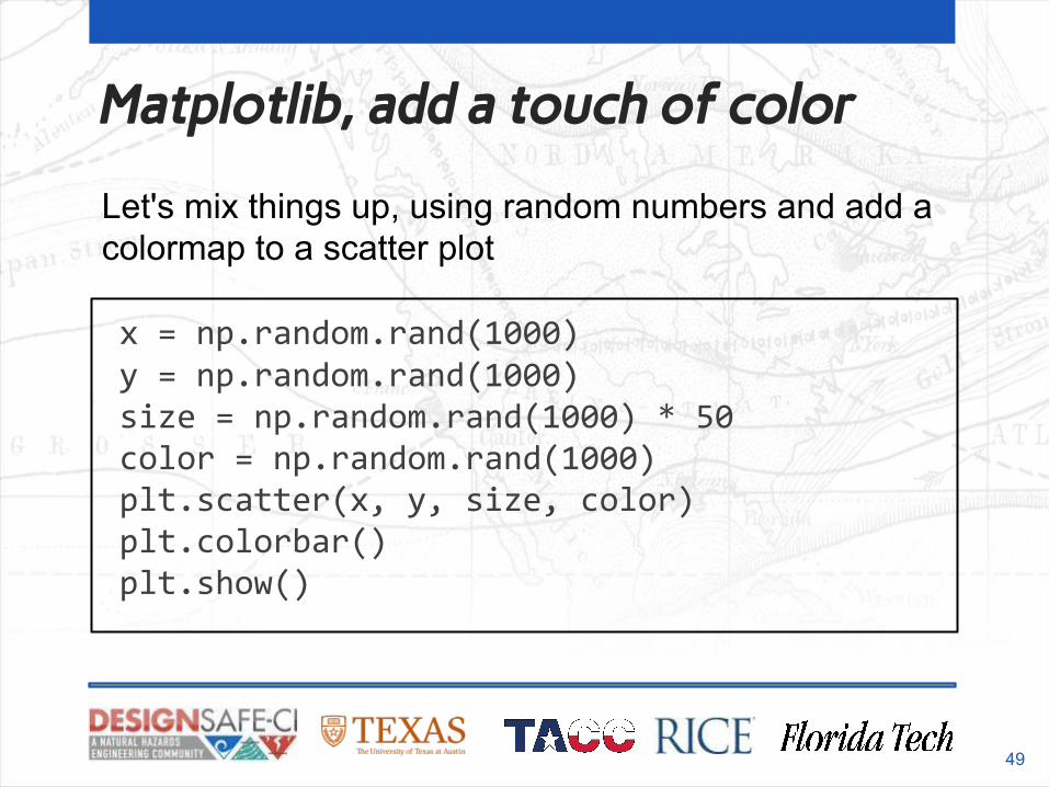
Matplotlib, add a touch of color

x = np.random.rand(1000)y = np.random.rand(1000)size = np.random.rand(1000) * 50color = np.random.rand(1000)plt.scatter(x, y, size, color)plt.colorbar()plt.show()

49

Let's mix things up, using random numbers and add a colormap to a scatter plot

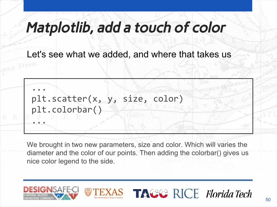
Matplotlib, add a touch of color

...plt.scatter(x, y, size, color)plt.colorbar()...

We brought in two new parameters, size and color. Which will varies the diameter and the color of our points. Then adding the colorbar() gives us nice color legend to the side.

50

Let's see what we added, and where that takes us

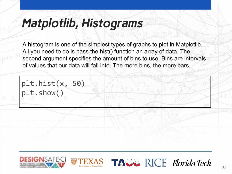
Matplotlib, Histograms

plt.hist(x, 50)plt.show()

51

A histogram is one of the simplest types of graphs to plot in Matplotlib. All you need to do is pass the hist() function an array of data. The second argument specifies the amount of bins to use. Bins are intervals of values that our data will fall into. The more bins, the more bars.

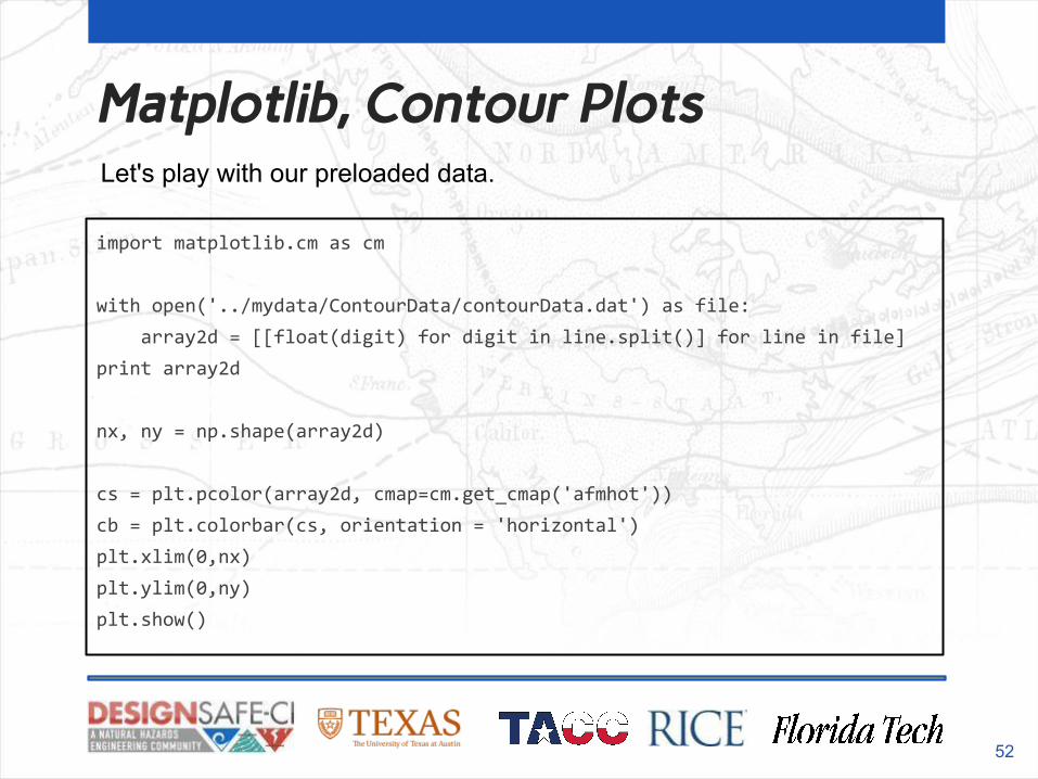
Matplotlib, Contour Plots

import matplotlib.cm as cm

with open('../mydata/ContourData/contourData.dat') as file:

array2d = [[float(digit) for digit in line.split()] for line in file]

print array2d

nx, ny = np.shape(array2d)

cs = plt.pcolor(array2d, cmap=cm.get_cmap('afmhot'))

cb = plt.colorbar(cs, orientation = 'horizontal')

plt.xlim(0,nx)

plt.ylim(0,ny)

plt.show()

52

Let's play with our preloaded data.

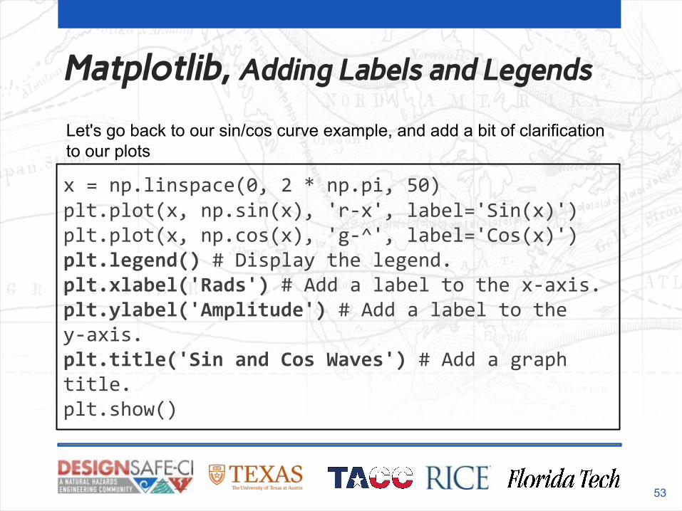
Matplotlib, Adding Labels and Legends

x = np.linspace(0, 2 * np.pi, 50)plt.plot(x, np.sin(x), 'r-x', label='Sin(x)')plt.plot(x, np.cos(x), 'g-^', label='Cos(x)')plt.legend() # Display the legend.plt.xlabel('Rads') # Add a label to the x-axis.plt.ylabel('Amplitude') # Add a label to the y-axis.plt.title('Sin and Cos Waves') # Add a graph title.plt.show()

53

Let's go back to our sin/cos curve example, and add a bit of clarification to our plots

DesignSafe: Questions?

54

For additional questions, feel free to contact us • Email:

training@designsafe-ci.org

• or fill out a ticket:https://www.designsafe-ci.org/help/tickets

An example.

presented by:Scott J. Brandenberg, Ph.D., P.E.Associate ProfessorDepartment of Civil and Environmental EngineeringUniversity of California

55

DesignSafe: Thanks

56

Ellen Rathje, Tim Cockerill, Jamie Padgett, Scott Brandenberg, Dan Stanzione, Steve Mock, Matt Hanlon, Josue Coronel, Manuel Rojas, Joe Stubbs, Matt Stelmaszek, Hedda Prochaska, Joonyee Chuah

DesignSafe: References

57

• http://www.datadependence.com/2016/04/scientific-python-matplotlib/• http://jupyter-notebook.readthedocs.io/en/latest/notebook.html• http://jupyter-notebook-beginner-guide.readthedocs.io/en/latest/what_is_jupyter.h

tml• https://github.com/adam-p/markdown-here/wiki/Markdown-Cheatsheet• https://www.codecademy.com/learn/python

DesignSafe: Next Webinar

58

For additional questions, feel free to contact us • Email:

training@designsafe-ci.org

• or fill out a ticket:https://www.designsafe-ci.org/help/tickets

DesignSafe: Data Analysis and Plotting usingJupyter and R

Wednesday, November 9th 1:00p – 3:00p