Embed Size (px)
Citation preview
ISSN: 1439-2305
Number 194 – September 2014
NATURAL DISASTERS AND
MACROECONOMIC PERFORMANCE:
THE ROLE OF RESIDENTIAL
INVESTMENT
Holger Strulik, Timo Trimborn
Natural Disasters and Macroeconomic Performance:
The Role of Residential Investment
Holger Strulik∗
Timo Trimborn∗∗
First Version: March 2014. This Version: September 2014
Abstract. Recent empirical research has shown that income per capita in the aftermath
of natural disasters is not necessarily lower than before the event. In many cases, income is
not significantly affected and surprisingly, can even respond positively to natural disasters.
Here, we propose a simple theory based on the neoclassical growth model that explains
these observations. Specifically, we show that GDP is driven above its pre-shock level
when natural disasters destroy predominantly residential housing (or other durable goods).
Disasters destroying mainly productive capital, in contrast, are predicted to reduce GDP.
Insignificant responses of GDP can be expected when disasters destroy about equally
residential structures and productive capital. We also show that disasters, irrespective of
whether their impact on GDP is positive, negative, or insignificant, entail considerable
losses of aggregate welfare.
Keywords: Natural Disasters; Economic Recovery; Residential Housing; Economic
Growth.
JEL: E20, O40, Q54, R31.
∗ University of Goettingen, Faculty of Economic Sciences, Platz der Goettinger Sieben 3, 37073, Goettingen,Germany, Email: [email protected]∗∗ University of Goettingen, Faculty of Economic Sciences, Platz der Goettinger Sieben 3, 37073, Goettingen,Germany, Email: [email protected]
1. Introduction
In this paper, we propose an economic theory to analyze the macroeconomic effects of natural
disasters. We mainly focus on hydro-meteorological disasters (e.g. floods, storms, droughts) and
geophysical disasters (e.g. earthquakes, tsunamis), and the physical and monetary damage caused
by these disasters. As documented by Cavallo and Noy (2011), these types of disasters are fairly
common events across the globe, and occur with increasing frequency. For example, in the Asia-
Pacific region, the most afflicted region, the incidence of natural disasters increased from 11 events
per country in the 1970s to 28 events in the 2000s. In Western Europe, events per country and
decade increased from 5 to 15 over the same time period.
To date, there exists a large and increasing empirical literature investigating the economic
impact of natural disasters (e.g. Raddatz, 2007; Noy, 2009; Loyza et al., 2012; Fomby et al.,
2013; Cavallo et al., 2013; see Cavallo and Noy, 2011 for a survey). One perhaps surprising
conclusion suggested by the literature is that disasters do not necessarily decrease GDP per capita
in the aftermath of the event. Loayza et al. (2012), for example, find no significant impact on a
country’s GDP and industrial output across all disasters. In contrast, when floods are investigated
separately, they are found to stimulate GDP while droughts are found to harm GDP in developing
countries (but not everywhere). Similarly, Fomby et al. (2013) find a positive effect of floods and
a negative effect of droughts but no effect of earthquakes and storms on post-disaster GDP in
developing countries. In developed countries, all types of disasters appear to exert no significant
impact on GDP. Using counterfactual analysis, Cavallo et al. (2013) find that disasters exert no
significant influence on short- and long-run output when they control for potential post-disaster
outbreak of social conflict.
These empirical observations seem puzzling when analyzed within the context of conventional
neoclassical growth theory. Once we acknowledge that disasters destroy (potentially severely)
the productive potential of an economy, we would expect that they then harm the subsequent
economic performance. It is true that the neoclassical growth model predicts that the growth rate
after an exogenous loss of capital stock (or other productive factors) is positive. This phenomenon
is known as catch-up growth from below towards the steady-state. GDP per capita, however, is
predicted to fall short of its pre-disaster level according to conventional growth theory.1
1The disaster literature, confusingly for growth economists, refers sometimes to the differential between pre- andpost-shock levels of GDP as GDP growth (e.g. Loayza et al., 2012). This differential is predicted by the standardneoclassical growth model to be unambiguously negative. Moreover there exists also a smaller literature investigating
1
In this paper, we show how a simple extension of the neoclassical growth model can be used
to reconcile theory with empirics and how the model can be used to motivate the diverse post-
shock macroeconomic outcomes found in the disaster literature. The key ingredients are the
introduction of variable labor supply and the distinction between productive capital stock and
residential housing (and other durable goods). In line with conventional theory, the model predicts
that an exogenous loss of capital stock reduces post-disaster GDP. An exogenous loss of residential
housing, in contrast, drives GDP above its pre-shock level. The reason is that individuals, suffering
from the implied wealth shock, supply more labor in order to (quickly) rebuild the damaged houses
(and other damaged durable goods such as cars). Since firm capital remained undestroyed, the
increased labor supply implies higher GDP per capita during the reconstruction phase.
Considering simultaneous shocks on both state variables, the model predicts a negative im-
pact on GDP for disasters destroying predominantly productive capital and a positive impact on
GDP for disasters destroying predominantly residential housing. No significant effect on GDP
is predicted when the effects on firm capital is slightly smaller compared to that on residential
housing. The theory is not only helpful to explain the frequently insignificant impact of disasters
on GDP, it can also rationalize those cases for which the literature finds significant GDP effects.
Intuitively, we may expect that droughts exert a negative impact on GDP because they leave
residential housing mostly intact and destroy predominantly firm capital. This is in particularly
the case in largely agrarian societies (seeds, livestock). Conversely, we could imagine that floods
stimulate GDP because they damage predominantly residential housing (and other durable goods,
like furniture or household appliances). Furthermore, some authors find positive employment ef-
fects of disasters supporting our proposed mechanism through which output might increase in the
aftermath of a disaster (see Leiter et al., 2009, Ewing et al., 2009).
In order to present the mechanics behind the “housing–channel” in the cleanest way we first
discuss in Section 3 the case of a small open economy with perfect capital mobility. This exercise
shuts down the “capital-channel” because capital stock is pinned down to its steady-state value.
In this framework, we generally prove that disasters damaging residential housing lead to higher
output in the short and long-run and we state conditions under which the response of GDP
is also positive. The reason for the positive effect on GDP is that disasters reduce the wealth
the association between disaster risk and long-run growth (e.g. Skidmore and Toya, 2002; and Crespo Cuaresma etal., 2008). Here, we focus on the short- to medium-run impact of disasters.
2
of households, which motivates them to supply more labor in order to quickly reconstruct the
damaged houses and durable goods.
We then turn to the large economy case and show that the main mechanics of the wealth effect
are preserved while another amplifying effect occurs through intertemporal substitution. House-
holds want to reconstruct their damaged houses quickly and increase their residential investments
in the aftermath of the disaster. Resources for this purpose are freed by reducing investments in
productive capital and by reducing consumption of nondurable goods. In order to mitigate the
drop in consumption, households are motivated to raise their labor supply even further, beyond
what has already been triggered by the wealth effect.
Our analysis of the individual effects of disasters on firm capital and on residential housing
shows that GDP can be a very misleading indicator of the economic damage caused by natural
disasters. This is most obvious when we compare a disaster that destroys “only” productive
capital with another one destroying additionally residential housing. The GDP damage is larger
for the first one while the welfare loss is larger for the second one. At the end of the paper, we
perform a welfare analysis for a numerically specified version of the model and find large welfare
losses from natural diasters that leave GDP more or less unaffected.
The paper is organized as follows. The next section introduces the general model. Section 3
presents the case of a small open economy and Section 4 presents the closed economy case. In the
main text, we assume that households own their houses. In the Appendix, we show robustness
of results against an alternative setup in which households rent housing services from firms. In
Section 5, we specify the model numerically and investigate post-disaster adjustment dynamics
quantitatively. We provide estimates of the incurred welfare loss under varying assumptions
about the physical impact of disasters. Throughout the paper we focus on economic or “material”
effects and ignore the fact that natural disasters kill people. The welfare estimates should thus
be understood as lower bounds of the actual damage caused by natural disasters.
2. The Model
2.1. Households. The economy is populated by a continuum (0, 1) of households who take prices
as given, supply ℓ units of labor, and experience utility from consuming nondurable goods c and
housing (and other durable goods) d as well as from enjoying leisure (1− ℓ). In order to keep the
3
utility function general, we abstain from introducing exogenous technological growth. As well-
known from the business cycle literature, introducing trend growth would entail severe restrictions
on the functional form of the utility function in order to guarantee that leisure is stationary. Our
variables (besides leisure) could be interpreted as being measured in terms of deviation from trend
growth. In order to derive theoretical results, we have to assume that utility is additively separable
between nondurable consumption, durable consumption, and leisure.2 In the quantitative part
of the paper, we also investigate non-separable utility and demonstrate robustness of the main
results.3
Households maximize lifetime utility
V =
∫
∞
0(u(c) + v(d) + q(1− ℓ)) · e−ρtdt, (1)
where u, v, and q denote concave sub-utility functions satisfying the Inada conditions and ρ is
the time preference rate. To simplify the notation, we introduce σc, σd, and σℓ as the inverse
of the elasticity of intertemporal substitution for nondurable goods consumption, durable goods
consumption, and leisure, respectively:
σc(c) := −c u′′(c)
u′(c)σd(d) := −
d v′′(d)
v′(d)σℓ(ℓ) := −
ℓ q′′(ℓ)
q′(ℓ). (2)
Household income is spent on nondurable consumption goods c and on residential investment x
(including potential investment in other durable goods). Households earn a wage w per unit of
labor supplied and hold assets a, on which they earn a return r, which altogether implies that
they face the budget constraint
a = wℓ+ ra− c− px , (3)
in which p denotes the price of residential investment. We assume that a no-Ponzi-game condition
for assets holds.
Durable goods depreciate at rate δd; hence, the stock of durables evolves according to
d = x− δdd , (4)
2Iacoviello (2005) argues that separability between nondurable and durable goods consumption is supported byempirical evidence; see also Bernanke (1984).3In this paper, we also neglect the influence of population growth and transportation costs on the economy and inparticular, on housing prices (see Knoll et al., 2014).
4
with x ≥ 0. Households choose c, ℓ, and x to maximize (1) subject to (3) and (4), and the initial
conditions a(0) = a0 and d(0) = d0. The first order conditions are
u′(c) = λ (5)
µ = pλ (6)
λw = q′(1− ℓ) (7)
λ = λρ− λr (8)
µ = µρ− v′(d) + µδ , (9)
where λ denotes the shadow price of one unit of installed capital in terms of marginal utility and
µ denotes the shadow price of one unit of residential housing in terms of marginal utility. From
the first order conditions we derive the Euler equation for consumption and a relation equating
the wage rate with the marginal rate of substitution between consumption of nondurables and
leisure:
c
c=r − ρ
σc(10)
w =q′(1− ℓ)
u′(c). (11)
2.2. Durable goods producing firms. There exists a continuum (0, 1) of construction firms
(firms producing durable goods). These firms convert units of final goods into units of housing
(durable goods). Following Iacoviello (2005) and Carlstrom and Fuerst (2010), we assume that
firms face convex adjustment costs depending on the amount of housing they produce per unit of
time. These costs can be understood as, for example, arising in terms of additional planning costs
when sequential tasks have to be performed in a tight time frame, or when there is inefficient labor
input due to fatigue during overtime hours. Since such costs arise when investment and thus the
workload is especially high, they explain why marginal costs are increasing in investment per unit
of time.
The empirical literature on capital and investment adjustment costs has identified costs arising
at the plant level if firms adjust the capital stock or investment (see e.g. Cooper and Haltiwanger,
2006, for a recent study). Similar costs are likely to emerge for firms in the residential construction
sector (see Topel and Rosen, 1988). In order to keep the analysis general, we assume that the
5
total costs for installing x units of housing sum up to x+ψ(x) with a convex function ψ satisfying
ψ(0) = 0. The literature on capital adjustment costs usually assumes that adjustment costs
additionally depend on the installed stock. For reasons of tractability we assume that costs
depend only on investment. Our quantitative results are robust against alternative specifications
with reasonable parametrization of adjustment costs.
Total firm revenue equals px. Each household is assumed to engage one construction firm per
unit of time but it can change the contracting party at any point of time. Free entry into the
construction sector implies that firms sell x at unit costs:
p = 1 +ψ(x)
x. (12)
Differentiating (12) with respect to time and using (5) – (9), we obtain the law of motion for
residential investment as
x
x=
(
ψ′(x)−ψ(x)
x
)
−1 [
p(r + δ) −v′(d)
u′(c)
]
. (13)
2.3. Final goods producing firms. The economy is populated by a continuum (0, 1) of firms
producing final goods. Final goods are used as nondurable consumption goods for residential
investment and for investment in firm capital. Each firm employs capital k and labor ℓ to produce
final output y = Af(k, ℓ), in which A denotes total factor productivity and f(k, ℓ) is a neoclassical
production function with positive and diminishing marginal returns. Firm capital depreciates at
rate δk. Firms hire labor and capital on competitive factor markets and pay them according to
their marginal product:
r =∂Af(k, ℓ)
∂k− δk , (14)
w =∂Af(k, ℓ)
∂ℓ. (15)
2.4. Output and GDP. In most macroeconomic models, aggregate output equals GDP. Here, in
a model with durable consumption goods, we have to distinguish between these aggregates. The
reason is that the System of National Accounts (SNA) requires counting the service flow from
already installed residential houses as part of consumption, and thus, it is part of GDP (see EC,
IMF, OECD, UN & World Bank, 2009, pp. 466-467). In particular, SNA states that houses leased
to other households are supposed to be treated equivalently to owner-occupied houses. A newly
6
constructed house raises output and GDP according to its construction costs. In the following
years, the house contributes to GDP – but not to output – according to the rent paid by its tenant
(if it is leased) or according to an imputed rent (if it is owner occupied). Houses are the only
durable goods from which a service flow enters GDP calculations. For example, service flows from
cars used for consumption purposes are not included as part of GDP.
In terms of our model, newly constructed houses are immediately part of output and GDP
since construction costs are paid from final output. Because houses are owner-occupied in our
benchmark model, we introduce an imputed rent in order to account for the contribution of
housing services to GDP. In Appendix B, we set up an alternative model in which houses are
leased to households by real estate firms. We show that the alternative setup is equivalent to the
benchmark model, and that the equilibrium rental price pd for renting one unit of d for one unit
of time is equal to
pd =v′(d)
u′(c). (16)
Intuitively, the price ratio between durable consumption goods and nondurable consumption
goods, pd/1, is equal to the marginal rate of substitution between durable consumption goods
and nondurable consumption goods, v′(d)/u′(c). In the following, we use (16) as the imputed
price for GDP accounting.
If durable goods d referred only to residential housing, GDP would be equal to output plus the
service flow from houses, GDP = y + pd · d. Here, we keep the analysis more general and leave
it open as to whether d refers only to housing or whether other durables such as cars, furniture,
and household appliances are included as well. We denote the share of housing in durable goods
by µ, 0 ≤ µ ≤ 1. This means that GDP is defined as
GDP = y + µ · pdd. (17)
The notation comprises two limiting cases: For µ = 1, durable goods consumption consists of only
housing and for µ = 0, durable goods consumption does not include any housing. Notice that
the latter case would capture as well countries deviating from the SNA rules by not including the
service flow of housing in their GDP accounts. We allow µ to take any number between zero and
one but mainly report results for the limiting cases µ = 0 and µ = 1. In other words, we provide
the upper and lower bounds for our GDP estimates.
7
3. The Small Open Economy
In a small open economy (and given perfect capital mobility) firms can borrow at the world
interest rate r, r = r. This means that equation (14) pins down the domestic capital labor ratio
and that the international wage rate, w = w, pins down the domestic wage in equation (15). In
order to simplify the formal analysis, we assume that r = ρ such that households prefer a constant
time profile of consumption and labor supply, c = ℓ = 0 (from equations (10) and (11)).
The demand for nondurable consumption goods and residential investment, as well as household
labor supply is determined by the intertemporal budget constraint. This means that any shock
or new information affecting the intertemporal budget constraint also affects the optimal level of
c and ℓ. The implied dynamics of residential investment is then given by equations (4) and (13).
In a small open economy, firm capital adjusts via international capital movements. We thus focus
the disaster analysis of this section on the effects originating from the destruction of residential
housing (and other durable goods). For this purpose, we assume that the economy rests at a
steady-state before it is hit by a natural disaster. In order to elaborate how the disaster affects
GDP, we begin by showing that the destruction of residential housing entails a negative wealth
effect. Households respond to the wealth shock by consuming fewer nondurables and housing
(and other durables) and by supplying more labor. Higher labor supply then lifts GDP above the
pre-shock level.
Integrating equation (3) provides the households’ intertemporal budget constraint,
∫
∞
0ce−rtdt = ℓ
∫
∞
0we−rtdt−
∫
∞
0p(x)xe−rtdt+ a0 . (18)
Using the fact that c and ℓ are constant, the budget constraint simplifies to
c
r=ℓw
r−
∫
∞
0p(x)xe−rtdt+ a0 . (19)
Finally, substituting w = v′(1− ℓ)/u′(c), we obtain
(u′)−1(
q′(1−ℓ)w
)
r−ℓw
r= a0 −
∫
∞
0p(x)xe−rtdt . (20)
Notice that the left-hand side of (20) depends negatively on ℓ since d (u′(·))−1/d(·) < 0. This
means that if households experience a negative wealth effect such that the right-hand side of (20)
decreases, the household will respond by supplying more labor.
8
We next show that an economy initially situated at a steady-state experiences indeed a negative
wealth effect when it is exposed to a disaster that destroys part of d. For that purpose we define
the net present value of residential investments as
X :=
∫
∞
0p(x)xe−rtdt =
∫
∞
0x
(
1 +ψ(x)
x
)
e−rtdt . (21)
Intuitively, a disaster that destroys parts of d, raises X, because rebuilding the stock of d requires
higher temporary investments x, which raises the net present value of future investments. In order
to verify this claim we focus on the dynamics of d and x summarized by
d = x− δdd (22)
x
x=
(
ψ′(x)−ψ(x)
x
)
−1 [(
1 +ψ(x)
x
)
(r + δd)−v′(d)
u′(c)
]
(23)
and d(0) = d0. The steady-state of the subsystem (22) and (23) is given by x = δdd and
(1 + ψ(x)/x) (r + δd) = v′(d)/u′(c). Notice that the steady-state of the subsystem depends on
c and that c is determined in conjunction with x by the intertemporal budget constraint (20) and
the labor supply equation (11). This means that the steady-state itself depends on the evolution
of the dynamic system towards the steady-state. In other words, the steady-state of the dynamic
subsystem (22) and (23) depends on the initial situation (c0, x0).4
In order to demonstrate that adjustment dynamics towards the steady-state are unique, we
construct a phase diagram, taking c as given and keeping in mind that c depends on X and
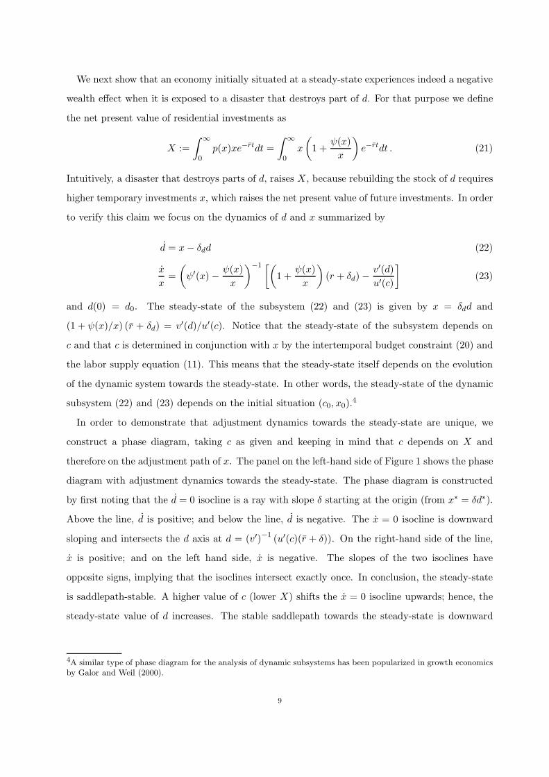
therefore on the adjustment path of x. The panel on the left-hand side of Figure 1 shows the phase
diagram with adjustment dynamics towards the steady-state. The phase diagram is constructed
by first noting that the d = 0 isocline is a ray with slope δ starting at the origin (from x∗ = δd∗).
Above the line, d is positive; and below the line, d is negative. The x = 0 isocline is downward
sloping and intersects the d axis at d = (v′)−1 (u′(c)(r + δ)). On the right-hand side of the line,
x is positive; and on the left hand side, x is negative. The slopes of the two isoclines have
opposite signs, implying that the isoclines intersect exactly once. In conclusion, the steady-state
is saddlepath-stable. A higher value of c (lower X) shifts the x = 0 isocline upwards; hence, the
steady-state value of d increases. The stable saddlepath towards the steady-state is downward
4A similar type of phase diagram for the analysis of dynamic subsystems has been popularized in growth economicsby Galor and Weil (2000).
9
sloping. In Appendix A we formally derive, that the subsystems (22) and (23) have a unique and
saddle-point stable steady-state.
Figure 1: Phase diagram
x
d
d=0
x=0
x∗= δd
∗
d∗
x
d
d=0
x=0
x∗
old
d∗
old
Left panel: Phase diagram with stable saddlepath. Right panel: Phase diagram used for proof ofLemma 1.
In comparison with conventional growth theory, the usual argument for uniqueness of adjust-
ment dynamics is slightly modified. To see this, consider an economy starting somewhere below
the stable saddlepath. Following the arrows of motion, the economy would always remain be-
low the saddlepath such that aggregate X would also be lower. Then, from the intertemporal
budget constraint (20), consumption c must be higher. This in turn means that the x = 0 iso-
cline, and thus the steady-state, shifts upwards. An economy starting below the stable saddlepath
would thus never arrive at the steady-state because x is below the stable saddlepath everywhere
during the transition and, secondly, because this very phenomenon shifts the steady-state even
further upwards. Analogously an economy starting above the saddlepath would never reach the
steady-state.5 This reasoning can be exploited to arrive at the following conclusion.
Lemma 1. If an economy rests at a steady-state and residential housing (d) gets destroyed,
aggregate expenditure on housing (X) increases compared to the pre-shock steady-state level.
Proof. The lemma is proved by contradiction. The counterfactual phase diagram is shown in
the panel on the right-hand side of Figure 1. Assume that the destruction of housing d reduces
5The local uniqueness of the saddlepath can also be proven by analyzing the full dynamic system. Numericalevaluation of the Jacobian matrix for a wide range of parameter values shows that it has one negative and one zeroeigenvalue. This indicates that the stable saddlepath is unique and that the steady-state to which the economyconverges depends on the initial conditions (a(0) = a0 and d(0) = d0).
10
aggregate housing expenditureX. In this case, equations (20) and (11) show that c would increase;
thus the x = 0 isocline would shift upwards. This would increase the steady-state value of d.
However, along the adjustment path, x is strictly larger than its former steady-state because the
stable saddlepath is downward sloping, x(t) > x∗old, implying increasing aggregate expenditure
X. In other words, reducing X in response to lower d would lead to a contradiction. If X would
remain constant, this would lead to a contradiction in an analogous way. In conclusion, after a
destruction of d, X rises compared to it original steady-state level. �
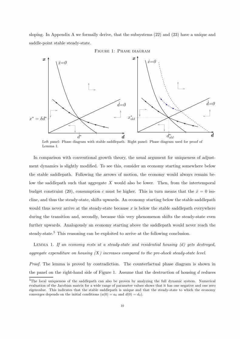
In short, the actual adjustment dynamics triggered by a natural disaster destroying d are shown
in Figure 2. Notice that along the adjustment path x is higher compared to the old steady-state
for an initial period [0, T ]. During the time interval (T,∞) x is smaller than x∗old. Yet due to
discounting of future expenditures and higher adjustment costs in the initial periods, X increases
in net terms. This leads to the following result.
Figure 2: Phase diagram: Adjustment Dynamics After Disaster
x
d
d=0
x=0
x∗
old
d∗
old
x∗
new
d∗
new
x(0)
d(0)
Proposition 1. If an economy rests at a steady-state and residential housing (d) gets destroyed,
only parts of the stock of d are rebuilt. The resulting new steady-state level of d is lower compared
to the pre-shock level.
Proof. Inspecting the adjustment dynamics derived in Figure 2 confirms that the after-shock
steady-state level of d lies below the pre-shock steady-state level. �
11
The result implies that without trend growth, an economy never completely rebuilds the housing
stock (stock of durables) destroyed by a disaster. If there is trend growth, d would grow at the
steady-state and the post-disaster growth rate of d would be higher than the pre-shock rate.
However, the level of d would be lower compared to an economy not experiencing the disaster and
growing along the balanced growth path.
The reason for the permanently lower level of residential housing is the negative wealth effect.
Households response to the diminished wealth by reducing their consumption of nondurable goods,
consumption of housing services (durable goods), and leisure. This leads to our next result.
Proposition 2. Aggregate welfare falls below its pre-shock level if residential housing gets
destroyed in an economy resting at a steady-state.
Proof. According to Proposition 1, the level of residential housing after the disaster falls perma-
nently below the pre-shock level. From Lemma 1, we conclude that consumption of nondurable
goods is also permanently lower. Finally, we conclude from equation (20) that labor supply in-
creases. Since instantaneous utility from all three components is strictly below pre-shock level,
the lifetime utility of households, i.e. aggregate welfare, is below the pre-shock level as well. �
Finally, we show that, although aggregate welfare is affected negatively, output and output
growth increase in response to the disaster, and we derive conditions under which GDP also
responds positively.
Proposition 3. If residential housing gets destroyed in an economy resting at a steady-state,
then aggregate output per capita increases permanently above the pre-shock level. Hence, output
growth in the aftermath of the disaster is positive.
Proof. If d gets destroyed, consumption of nondurable goods decreases (see equation (11)) and
labor supply increases (see equation (20)). Higher labor supply triggers capital inflows from the
rest of the world until the capital labor ratio reaches its pre-shock level and the domestic interest
rate equals the world interest rate. Higher labor supply in conjunction with higher capital stock
implies higher aggregate output per capita. �
The response of GDP in the aftermath of a disaster is equivalent to the response of output
only if µ = 0, i.e. if durable goods do not include residential housing. For µ > 0, GDP is also
affected by the service flow from residential housing, pdd, since GDP = y + µ · pdd. To evaluate
12
the full impact of disasters on GDP we need to show how the price of housing services pd responds
in relation to the destruction of residential houses d. Intuitively, the price of nondurable goods
relative to durable goods (and thus pd) increases when a disaster destroys the stock of durables.
Formally, the price is pinned down by (16). As long as we keep the utility function general, the
combined effect of disasters on pdd remains indeterminate. However, if the share of residential
housing in durables, µ, is sufficiently small, the effect of the disaster on output dominates the
service flows of housing. This leads to our final result.
Proposition 4. If residential housing gets destroyed in an economy resting at a steady-state,
then aggregate GDP per capita increases permanently above the pre-shock level if the share of
residential housing on durables, µ, is sufficiently small. In this case, GDP growth in the aftermath
of the disaster is positive.
Proof. We already verified that output responds positively in the aftermath of a disaster. If the
service flow of housing, pd · d, also responds positively, the result holds for any µ, 0 ≤ µ ≤ 1. If
pd · d responds negatively it is always possible to find a µ∗ such that the response of output is
equal to the response of µ ·pdd in absolute terms, i.e. |∆y| = µ∗ · |∆pd ·∆d|. Then, for any µ < µ∗,
GDP responds positively in the aftermath of a disaster. �
4. The Closed Economy Case
4.1. Setup of the Model. The closed economy model can be best understood as the standard
neoclassical growth model augmented by a housing sector and variable labor supply. In a closed
economy, households save only in terms of domestic capital such that a = k. The feature of
diminishing marginal returns to capital provides a unique steady-state.6
The households’ budget constraint (3) can be converted into an equation of motion for aggre-
gate capital by substituting factor prices (equations (14) and (15)) and the price of residential
investment (equation (12)). This provides (24). The remaining equations are shared with the
small open economy case. For convenience we again collect the decisive equations and obtain the
large economy as described by the following dynamic system
k = Af(k, ℓ)− δkk − x− ψ(x)− c (24)
6In the Appendix, we show that the dynamic system (22)–(26) has a unique steady-state. We also checked bynumerically evaluating the eigenvalues that adjustment dynamics are unique for the relevant range of parametervalues.
13
d = x− δd (25)
c
c=r − ρ
σc(26)
x
x=
(
ψ′(x)−ψ(x)
x
)
−1 [
p(r + δ) −v′(d)
u′(c)
]
(27)
w =q′(1− ℓ)
u′(c), (28)
together with initial conditions k(0) = k0 and d(0) = d0.
4.2. Effect of Disasters on GDP: Intuition. To illustrate out argument, we distinguish be-
tween two polar types of disasters. The first type destroys only residential housing (durable
consumption) while the second type destroys only productive capital. In reality, of course, disas-
ters usually destroy both d and k. Real disasters can be conceptualized as a mix of the two polar
cases. In the quantitative section, we first show results for the two polar types of disasters and
then investigate the impact of “mixed disasters”.
We begin the analysis again by inspecting the intertemporal budget constraint. Integrating (3)
and inserting a0 = k0, we obtain
∫
∞
0c e−
∫s
0r(u)duds = k0 +
∫
∞
0wℓ e−
∫s
0r(u)duds−
∫
∞
0p(x)xe−
∫s
0r(u)duds. (29)
The intertemporal budget constraint differs from the open economy case (equation 20) mainly
because the wage rate w and the interest rate r are now varying over time. A damaged stock of
productive capital entails temporarily lower wages and higher interest rates and these changing
factor prices impinge on household wealth. As demonstrated below, these “factor price effects” are
quantitatively of second order compared to the wealth effect originating from the loss of productive
capital or residential housing.
We start by analyzing a d-shock. As for the small open economy, destroyed houses entail recon-
struction costs such that the present value of aggregate residential investment∫
∞
0 p(x)xe−∫s
0r(u)duds
increases. This, in turn, implies lower household wealth. Households respond to the reduced
wealth by lowering consumption of nondurable goods and by supplying more labor. Productive
capital, by assumption, was not affected by the disaster, which means that higher labor supply
and employment lifts output above its pre-shock level. This also lifts GDP above its pre-shock
level, because the service flow from housing responds either positively or only slightly negatively
as we show below.
14
The impact of a disaster destroying productive capital can be investigated analogously. The
k-shock reduces k0 on the right-hand side of equation (29) and thus entails a negative wealth
effect as well. Households respond by consuming less nondurable goods, by reducing residential
investment, and by supplying more labor. The reason for this joint response lies in the fact that
nondurables, durables, and leisure are normal goods such that the demand for all three components
shifts in the same direction after a wealth shock. In contrast to the d-shock, higher labor supply
is not sufficient to lift output above the steady-state level for reasonable parameter values because
the lower level of capital after the shock is the dominant force on output. Instead, neoclassical
adjustment dynamics are induced: The economy starts at a lower level of output and converges
towards the steady-state from below.
The effect of a k-shock on the service flow of housing is also negative, amplifying the nega-
tive response of output. Intuitively, lower output forces households to reduce consumption of
nondurables in the aftermath of a k-disaster, which raises the marginal utility from nondurable
consumption. Since marginal utility from durable goods is not affected immediately after the
disaster, the rental price of durables pd declines. GDP responds negatively to the disaster because
output as well as service flows from housing decline. In order to verify this claim and to investigate
the quantitative effects of disasters, we continue with a numerical specification of the model.
5. Quantitative Analysis
5.1. Numerical Specification of the Model. In order to parameterize the model, we need to
specify the form of the utility function and the production technology. We assume that households
face an isoelastic utility function
∫
∞
0
[
c1−σc − 1
1− σc+ β
d1−σd − 1
1− σd+ η
(1− ℓ)1−σℓ − 1
1− σℓ
]
· e−ρtdt (30)
in which β and η denote the weights of residential housing and leisure, respectively. In Section
5.4, we relax the assumption of separable utility between nondurable and durable consumption
goods and verify that the results hold for non-separable utility as well. Firms are assumed to
produce according to the Cobb-Douglas production technology y = Akαℓ1−α, in which α denotes
the elasticity of output with respect to capital. Adjustment costs for residential investment are
assumed to be quadratic, i.e. ψ(x) = γx2.
15
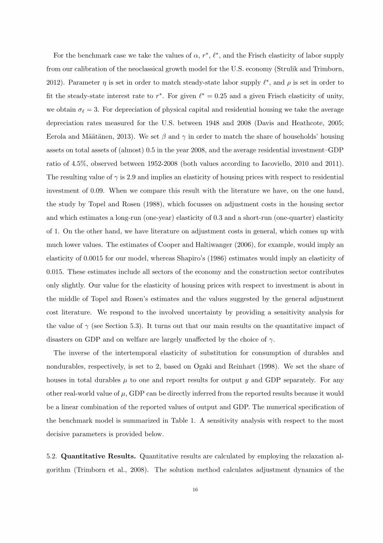
For the benchmark case we take the values of α, r∗, ℓ∗, and the Frisch elasticity of labor supply
from our calibration of the neoclassical growth model for the U.S. economy (Strulik and Trimborn,
2012). Parameter η is set in order to match steady-state labor supply ℓ∗, and ρ is set in order to
fit the steady-state interest rate to r∗. For given ℓ∗ = 0.25 and a given Frisch elasticity of unity,
we obtain σℓ = 3. For depreciation of physical capital and residential housing we take the average
depreciation rates measured for the U.S. between 1948 and 2008 (Davis and Heathcote, 2005;
Eerola and Maatanen, 2013). We set β and γ in order to match the share of households’ housing
assets on total assets of (almost) 0.5 in the year 2008, and the average residential investment–GDP
ratio of 4.5%, observed between 1952-2008 (both values according to Iacoviello, 2010 and 2011).
The resulting value of γ is 2.9 and implies an elasticity of housing prices with respect to residential
investment of 0.09. When we compare this result with the literature we have, on the one hand,
the study by Topel and Rosen (1988), which focusses on adjustment costs in the housing sector
and which estimates a long-run (one-year) elasticity of 0.3 and a short-run (one-quarter) elasticity
of 1. On the other hand, we have literature on adjustment costs in general, which comes up with
much lower values. The estimates of Cooper and Haltiwanger (2006), for example, would imply an
elasticity of 0.0015 for our model, whereas Shapiro’s (1986) estimates would imply an elasticity of
0.015. These estimates include all sectors of the economy and the construction sector contributes
only slightly. Our value for the elasticity of housing prices with respect to investment is about in
the middle of Topel and Rosen’s estimates and the values suggested by the general adjustment
cost literature. We respond to the involved uncertainty by providing a sensitivity analysis for
the value of γ (see Section 5.3). It turns out that our main results on the quantitative impact of
disasters on GDP and on welfare are largely unaffected by the choice of γ.
The inverse of the intertemporal elasticity of substitution for consumption of durables and
nondurables, respectively, is set to 2, based on Ogaki and Reinhart (1998). We set the share of
houses in total durables µ to one and report results for output y and GDP separately. For any
other real-world value of µ, GDP can be directly inferred from the reported results because it would
be a linear combination of the reported values of output and GDP. The numerical specification of
the benchmark model is summarized in Table 1. A sensitivity analysis with respect to the most
decisive parameters is provided below.
5.2. Quantitative Results. Quantitative results are calculated by employing the relaxation al-
gorithm (Trimborn et al., 2008). The solution method calculates adjustment dynamics of the
16
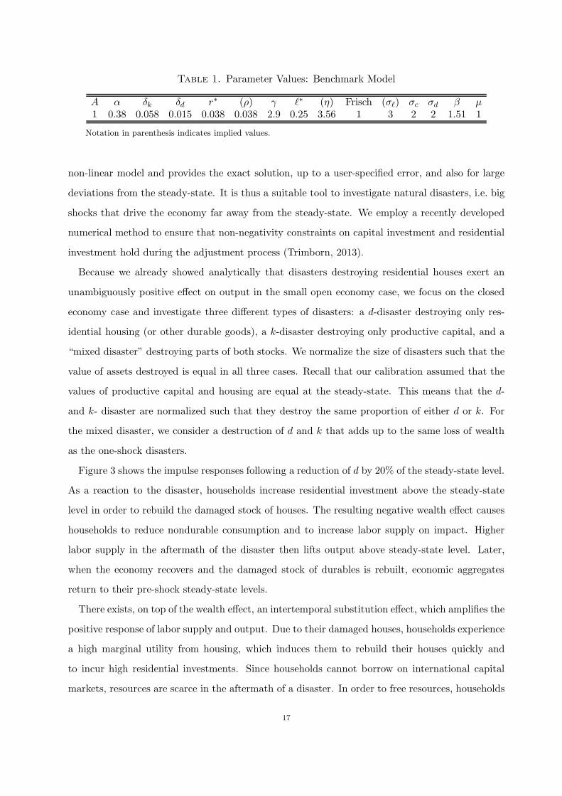
Table 1. Parameter Values: Benchmark Model
A α δk δd r∗ (ρ) γ ℓ∗ (η) Frisch (σℓ) σc σd β µ1 0.38 0.058 0.015 0.038 0.038 2.9 0.25 3.56 1 3 2 2 1.51 1
Notation in parenthesis indicates implied values.
non-linear model and provides the exact solution, up to a user-specified error, and also for large
deviations from the steady-state. It is thus a suitable tool to investigate natural disasters, i.e. big
shocks that drive the economy far away from the steady-state. We employ a recently developed
numerical method to ensure that non-negativity constraints on capital investment and residential
investment hold during the adjustment process (Trimborn, 2013).
Because we already showed analytically that disasters destroying residential houses exert an
unambiguously positive effect on output in the small open economy case, we focus on the closed
economy case and investigate three different types of disasters: a d-disaster destroying only res-
idential housing (or other durable goods), a k-disaster destroying only productive capital, and a
“mixed disaster” destroying parts of both stocks. We normalize the size of disasters such that the
value of assets destroyed is equal in all three cases. Recall that our calibration assumed that the
values of productive capital and housing are equal at the steady-state. This means that the d-
and k- disaster are normalized such that they destroy the same proportion of either d or k. For
the mixed disaster, we consider a destruction of d and k that adds up to the same loss of wealth
as the one-shock disasters.
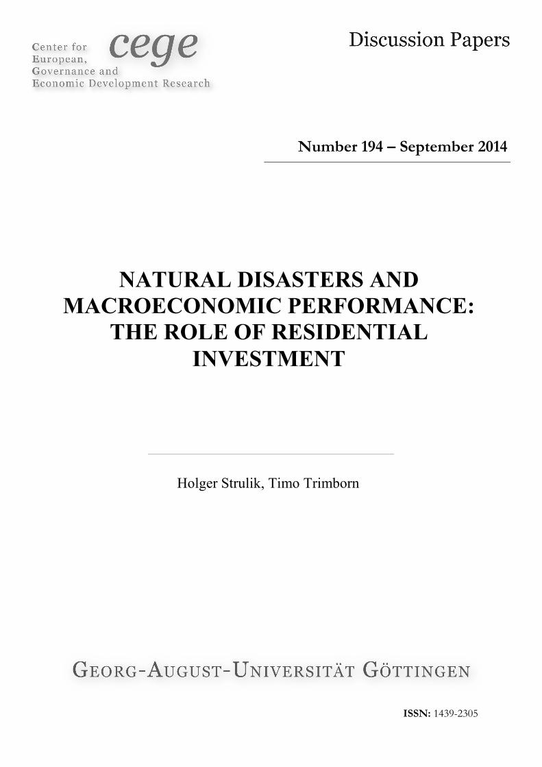
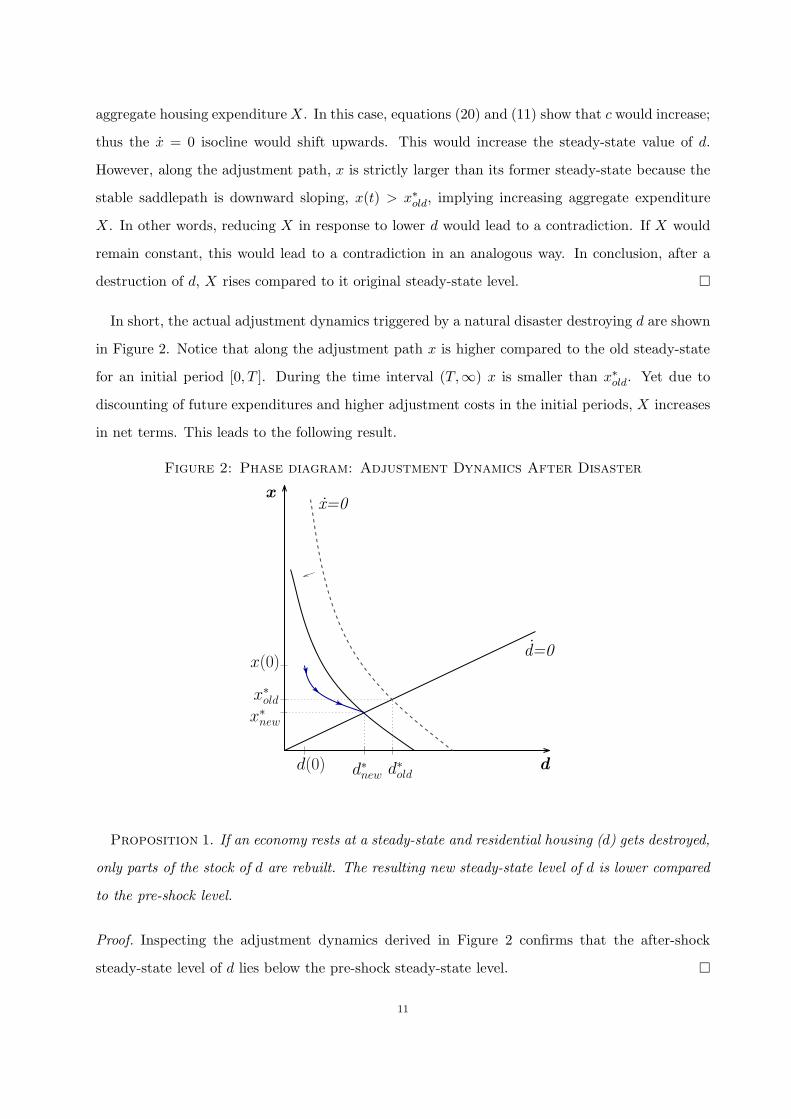
Figure 3 shows the impulse responses following a reduction of d by 20% of the steady-state level.
As a reaction to the disaster, households increase residential investment above the steady-state
level in order to rebuild the damaged stock of houses. The resulting negative wealth effect causes
households to reduce nondurable consumption and to increase labor supply on impact. Higher
labor supply in the aftermath of the disaster then lifts output above steady-state level. Later,
when the economy recovers and the damaged stock of durables is rebuilt, economic aggregates
return to their pre-shock steady-state levels.
There exists, on top of the wealth effect, an intertemporal substitution effect, which amplifies the
positive response of labor supply and output. Due to their damaged houses, households experience
a high marginal utility from housing, which induces them to rebuild their houses quickly and
to incur high residential investments. Since households cannot borrow on international capital
markets, resources are scarce in the aftermath of a disaster. In order to free resources, households
17

Figure 3: Natural Disasters: Destruction of Residential Housing
0 10 20 30
0.98
0.99
1
years
k
0 10 20 30
0.8
0.9
1
years
d
0 10 20 30
1
1.4
1.8
2.2
years
x
0 10 20 30
0.97
0.98
0.99
1
years
c
0 10 20 30
0.25
0.255
0.26
years
l
0 10 20 30
0.96
0.98
1
1.02
years
y
0 10 20 30
1
1.2
1.4
years
pd
0 10 20 30
0.95
1
1.05
years
GDP
Impulse responses to the destruction of residential housing by 20%. The panel shows the response of capital (k),residential housing (d), residential investment (x), nondurable consumption (c), labor supply (ℓ), rental price ofdurables (pd), output (y), and GDP (for µ = 1).
reduce capital investment and consumption. Then, in order to mitigate the drop in consumption,
households further increase their labor supply in the aftermath of the disaster. As a consequence,
output in the initial periods after the disaster rises even further, beyond the increase triggered by
the wealth effect.
To assess the impact on GDP, recall that GDP equals output plus the service flow from housing,
pd · d. A smaller stock of housing in the aftermath of the disaster has a negative impact on
GDP, whereas a higher price of housing services, pd, has a positive impact. For our numerical
specification of the model it turns out that the price effect dominates the quantity effect such that
GDP reacts even more strongly than output (see panel for pd, y, and GDP in Figure 3).
As a side effect, lower investment in productive capital reduces the capital stock. Only after
about nine years – when about half of the houses and other durable goods have been reconstructed
– investment in capital is higher than depreciation and the capital stock returns to its steady-state
level from below.
In our numerical simulations it turns out that as long as the Frisch elasticity of labor supply
is positive, the initial response of labor supply and hence of output and GDP is positive. The
sensitivity analysis conducted in Section 5.3 shows that even for small Frisch elasticities, GDP
responds positively to disasters destroying residential housing. The sensitivity analysis also re-
veals that the relative magnitude of the intertemporal elasticity of substitution for nondurable
18
consumption and durable consumption determines the size of the intertemporal substitution ef-
fect and therefore, much of the quantitative response of output. As a rule, the positive response of
output is stronger when the intertemporal elasticity of substitution for nondurable consumption
and durable consumption is low (high σc and σd), respectively. We explain the mechanism behind
this finding in more detail in the next section.
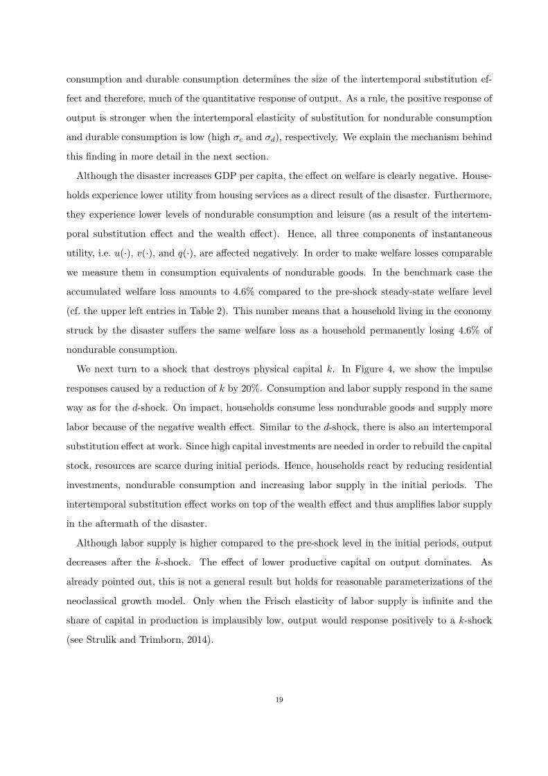
Although the disaster increases GDP per capita, the effect on welfare is clearly negative. House-
holds experience lower utility from housing services as a direct result of the disaster. Furthermore,
they experience lower levels of nondurable consumption and leisure (as a result of the intertem-
poral substitution effect and the wealth effect). Hence, all three components of instantaneous
utility, i.e. u(·), v(·), and q(·), are affected negatively. In order to make welfare losses comparable
we measure them in consumption equivalents of nondurable goods. In the benchmark case the
accumulated welfare loss amounts to 4.6% compared to the pre-shock steady-state welfare level
(cf. the upper left entries in Table 2). This number means that a household living in the economy
struck by the disaster suffers the same welfare loss as a household permanently losing 4.6% of
nondurable consumption.
We next turn to a shock that destroys physical capital k. In Figure 4, we show the impulse
responses caused by a reduction of k by 20%. Consumption and labor supply respond in the same
way as for the d-shock. On impact, households consume less nondurable goods and supply more
labor because of the negative wealth effect. Similar to the d-shock, there is also an intertemporal
substitution effect at work. Since high capital investments are needed in order to rebuild the capital
stock, resources are scarce during initial periods. Hence, households react by reducing residential
investments, nondurable consumption and increasing labor supply in the initial periods. The
intertemporal substitution effect works on top of the wealth effect and thus amplifies labor supply
in the aftermath of the disaster.
Although labor supply is higher compared to the pre-shock level in the initial periods, output
decreases after the k-shock. The effect of lower productive capital on output dominates. As
already pointed out, this is not a general result but holds for reasonable parameterizations of the
neoclassical growth model. Only when the Frisch elasticity of labor supply is infinite and the
share of capital in production is implausibly low, output would response positively to a k-shock
(see Strulik and Trimborn, 2014).
19
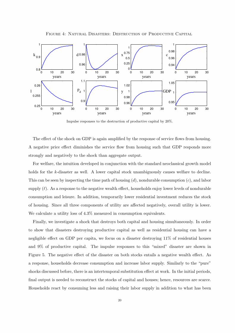
Figure 4: Natural Disasters: Destruction of Productive Capital
0 10 20 30
0.8
0.9
1
years
k
0 10 20 30
0.96
0.98
1
years
d
0 10 20 30
0
0.25
0.5
0.75
1
years
x
0 10 20 30
0.94
0.96
0.98
1
years
c
0 10 20 30
0.25
0.255
0.26
years
l
0 10 20 30
0.96
0.98
1
1.02
years
y
0 10 20 30
0.9
1
1.1
years
pd
0 10 20 30
0.95
1
1.05
years
GDP
Impulse responses to the destruction of productive capital by 20%.
The effect of the shock on GDP is again amplified by the response of service flows from housing.
A negative price effect diminishes the service flow from housing such that GDP responds more
strongly and negatively to the shock than aggregate output.
For welfare, the intuition developed in conjunction with the standard neoclassical growth model
holds for the k-disaster as well. A lower capital stock unambiguously causes welfare to decline.
This can be seen by inspecting the time path of housing (d), nondurable consumption (c), and labor
supply (ℓ). As a response to the negative wealth effect, households enjoy lower levels of nondurable
consumption and leisure. In addition, temporarily lower residential investment reduces the stock
of housing. Since all three components of utility are affected negatively, overall utility is lower.
We calculate a utility loss of 4.3% measured in consumption equivalents.
Finally, we investigate a shock that destroys both capital and housing simultaneously. In order
to show that disasters destroying productive capital as well as residential housing can have a
negligible effect on GDP per capita, we focus on a disaster destroying 11% of residential houses
and 9% of productive capital. The impulse responses to this “mixed” disaster are shown in
Figure 5. The negative effect of the disaster on both stocks entails a negative wealth effect. As
a response, households decrease consumption and increase labor supply. Similarly to the “pure”
shocks discussed before, there is an intertemporal substitution effect at work. In the initial periods,
final output is needed to reconstruct the stocks of capital and houses; hence, resources are scarce.
Households react by consuming less and raising their labor supply in addition to what has been
20
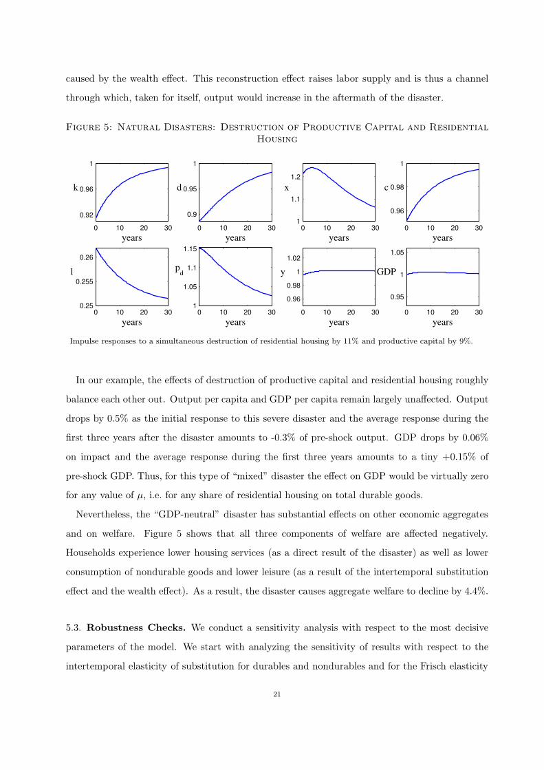
caused by the wealth effect. This reconstruction effect raises labor supply and is thus a channel
through which, taken for itself, output would increase in the aftermath of the disaster.
Figure 5: Natural Disasters: Destruction of Productive Capital and Residential
Housing
0 10 20 30
0.92
0.96
1
years
k
0 10 20 30
0.9
0.95
1
years
d
0 10 20 30
1
1.1
1.2
years
x
0 10 20 30
0.96
0.98
1
years
c
0 10 20 30
0.25
0.255
0.26
years
l
0 10 20 30
0.96
0.98
1
1.02
years
y
0 10 20 30
1
1.05
1.1
1.15
years
pd
0 10 20 30
0.95
1
1.05
years
GDP
Impulse responses to a simultaneous destruction of residential housing by 11% and productive capital by 9%.
In our example, the effects of destruction of productive capital and residential housing roughly
balance each other out. Output per capita and GDP per capita remain largely unaffected. Output
drops by 0.5% as the initial response to this severe disaster and the average response during the
first three years after the disaster amounts to -0.3% of pre-shock output. GDP drops by 0.06%
on impact and the average response during the first three years amounts to a tiny +0.15% of
pre-shock GDP. Thus, for this type of “mixed” disaster the effect on GDP would be virtually zero
for any value of µ, i.e. for any share of residential housing on total durable goods.
Nevertheless, the “GDP-neutral” disaster has substantial effects on other economic aggregates
and on welfare. Figure 5 shows that all three components of welfare are affected negatively.
Households experience lower housing services (as a direct result of the disaster) as well as lower
consumption of nondurable goods and lower leisure (as a result of the intertemporal substitution
effect and the wealth effect). As a result, the disaster causes aggregate welfare to decline by 4.4%.
5.3. Robustness Checks. We conduct a sensitivity analysis with respect to the most decisive
parameters of the model. We start with analyzing the sensitivity of results with respect to the
intertemporal elasticity of substitution for durables and nondurables and for the Frisch elasticity
21
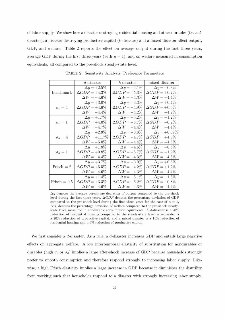
of labor supply. We show how a disaster destroying residential housing and other durables (i.e. a d-
disaster), a disaster destroying productive capital (k-disaster) and a mixed disaster affect output,
GDP, and welfare. Table 2 reports the effect on average output during the first three years,
average GDP during the first three years (with µ = 1), and on welfare measured in consumption
equivalents, all compared to the pre-shock steady-state level.
Table 2. Sensitivity Analysis: Preference Parameters
d-disaster k-disaster mixed-disaster
benchmark∆y=+2.5% ∆y=−4.1% ∆y=−0.3%
∆GDP =+4.3% ∆GDP =−5.3% ∆GDP =+0.2%∆W =−4.6% ∆W =−4.3% ∆W =−4.4%
σc = 4∆y=+3.0% ∆y=−3.3% ∆y=+0.4%
∆GDP =+4.6% ∆GDP =−4.9% ∆GDP =+0.5%∆W =−4.4% ∆W =−4.2% ∆W =−4.2%
σc = 1∆y=+1.7% ∆y=−5.2% ∆y=−1.2%
∆GDP =+4.0% ∆GDP =−5.7% ∆GDP =−0.2%∆W =−4.7% ∆W =−4.4% ∆W =−4.4%
σd = 4∆y=+2.9% ∆y=−3.8% ∆y=+0.09%
∆GDP =+11.7% ∆GDP =−4.7% ∆GDP =+4.0%∆W =−5.0% ∆W =−4.4% ∆W =−4.5%
σd = 1∆y=+1.8% ∆y=−4.6% ∆y=−0.8%
∆GDP =+0.8% ∆GDP =−5.7% ∆GDP =−1.9%∆W =−4.4% ∆W =−4.3% ∆W =−4.3%
Frisch = 2∆y=+3.7% ∆y=−3.0% ∆y=+0.8%
∆GDP =+5.5% ∆GDP =−4.2% ∆GDP =+1.2%∆W =−4.6% ∆W =−4.3% ∆W =−4.4%
Frisch = 0.5∆y=+1.4% ∆y=−5.1% ∆y=−1.3%
∆GDP =+3.3% ∆GDP =−6.2% ∆GDP =−0.8%∆W =−4.6% ∆W =−4.3% ∆W =−4.4%
∆y denotes the average percentage deviation of output compared to the pre-shocklevel during the first three years, ∆GDP denotes the percentage deviation of GDPcompared to the pre-shock level during the first three years for the case of µ = 1,∆W denotes the percentage deviation of welfare compared to the pre-shock steady-state level, measured in nondurable consumption equivalents. A d-disaster is a 20%reduction of residential housing compared to the steady-state level, a k-disaster isa 20% reduction of productive capital, and a mixed disaster is a 11% reduction ofresidential housing and a 9% reduction of productive capital.
We first consider a d-disaster. As a rule, a d-disaster increases GDP and entails large negative
effects on aggregate welfare. A low intertemporal elasticity of substitution for nondurables or
durables (high σc or σd) implies a large after-shock increase of GDP because households strongly
prefer to smooth consumption and therefore respond strongly to increasing labor supply. Like-
wise, a high Frisch elasticity implies a large increase in GDP because it diminishes the disutility
from working such that households respond to a disaster with strongly increasing labor supply.
22
Altogether, output rises between 1.4 and 3.7 percent and GDP rises between 0.8 percent and 11.7
percent for the considered range of elasticities. At the same time, variations of the intertemporal
elasticity of substitution for nondurables and durables as well as variations of the Frisch elasticity
have a relatively small impact on the estimated welfare loss, which is always around 5 percent.
A k-disaster (column two of Table 2) always exerts a negative effect on GDP during the first
three years and a drastic negative effect on aggregate welfare. A lower intertemporal elasticity
of substitution for nondurables or durables (higher σc or σd) reduces the initial response of GDP
because households prefer to smooth consumption more strongly, thereby increasing their labor
supply more strongly. Likewise, households increase labor supply in the aftermath of a disaster
particularly strongly when the Frisch elasticity is high. Again, the size of the preference parameters
has a relatively small impact on the estimated welfare loss.
A mixed disaster (column three of Table 2) has an insignificant impact on output and GDP
but a significantly negative impact on welfare. The effect on welfare is comparable in magnitude
to the one obtained for the d-disasters and k-disasters. The effect on output is mildly positive
when preferences imply a high response of labor supply (i.e. for high σc, σc, or Frisch elasticity),
and mildly negative otherwise. Notice, however, that it is always possible to identify an “output-
neutral” and a “GDP-neutral” disaster for any choice of the preference parameters. In other
words, there is always a disaster for which the positive labor supply effect and the negative effect
on productive capital balance each other out.
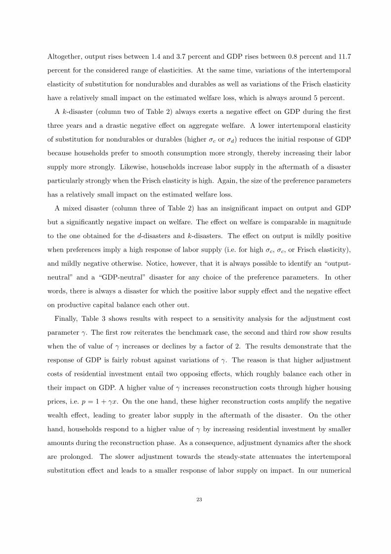
Finally, Table 3 shows results with respect to a sensitivity analysis for the adjustment cost
parameter γ. The first row reiterates the benchmark case, the second and third row show results
when the of value of γ increases or declines by a factor of 2. The results demonstrate that the
response of GDP is fairly robust against variations of γ. The reason is that higher adjustment
costs of residential investment entail two opposing effects, which roughly balance each other in
their impact on GDP. A higher value of γ increases reconstruction costs through higher housing
prices, i.e. p = 1 + γx. On the one hand, these higher reconstruction costs amplify the negative
wealth effect, leading to greater labor supply in the aftermath of the disaster. On the other
hand, households respond to a higher value of γ by increasing residential investment by smaller
amounts during the reconstruction phase. As a consequence, adjustment dynamics after the shock
are prolonged. The slower adjustment towards the steady-state attenuates the intertemporal
substitution effect and leads to a smaller response of labor supply on impact. In our numerical
23
experiments it turns out that the expansive and contractive forces roughly balance each other out
such that the response of GDP is largely unaffected by the size of γ. Only for very small values
of γ does the average response of GDP during the first three years become less pronounced, while
at the same time, the response on impact becomes very large (not shown in Table 3).
Table 3. Sensitivity Analysis: Adjustment Costs
d-disaster k-disaster mixed-disaster
γ = 2.9 ǫ = 0.09∆y=+2.5% ∆y=−4.1% ∆y=−0.3%
∆GDP =+4.3% ∆GDP =−5.3% ∆GDP =+0.2%∆W =−4.6% ∆W =−4.3% ∆W =−4.4%
γ = 5.7 ǫ = 0.17∆y=+2.4% ∆y=−4.1% ∆y=−0.04%
∆GDP =+5.2% ∆GDP =−4.9% ∆GDP =+0.8%∆W =−5.0% ∆W =−4.3% ∆W =−4.5%
γ = 1.5 ǫ = 0.05∆y=+2.4% ∆y=−4.1% ∆y=+0.1%
∆GDP =+3.7% ∆GDP =−5.3% ∆GDP =+0.4%∆W =−4.4% ∆W =−4.3% ∆W =−4.3%
γ = 0.45 ǫ = 0.015∆y=+2.2% ∆y=−3.6% ∆y=+0.1%
∆GDP =+2.7% ∆GDP =−4.7% ∆GDP =+0.02%∆W =−4.2% ∆W =−4.3% ∆W =−4.2%
γ = 0.05 ǫ = 0.0015∆y=+1.0% ∆y=−1.9% ∆y=+0.00%
∆GDP =+1.0% ∆GDP =−2.5% ∆GDP =−0.3%∆W =−4.1% ∆W =−4.3% ∆W =−4.2%
ǫ is the implied price elasticity of housing investment. See Table 2 for further notes.
Table 3 also demonstrates that variations in the size of γ only mildly affect the estimated welfare
loss. The effect of k-disasters on welfare is insignificantly influenced by the choice of γ. For d-
disasters and mixed disasters, we obtain a somewhat larger welfare loss for high values of γ. The
reason is, again, that large adjustment costs prolong adjustment dynamics. A higher value of γ
leads to a slower and more costly reconstruction of houses. This means that the stock of houses is
below its long-run optimal value for a longer period of time, an outcome that increases the welfare
loss.
Interestingly, these conclusions remain valid when we further reduce γ towards values close to
zero, implying a price elasticity of residential investment equal to what have been suggested by
Shapiro (1986) and Cooper and Haltiwanger (2006); see the discussion in Section 5.1. Results
are documented in row 4 and 5 of Table 3. In particular, our main result of substantial welfare
losses from GDP-neutral disasters turns out to be also quantitatively robust against the size of
adjustment costs.
24
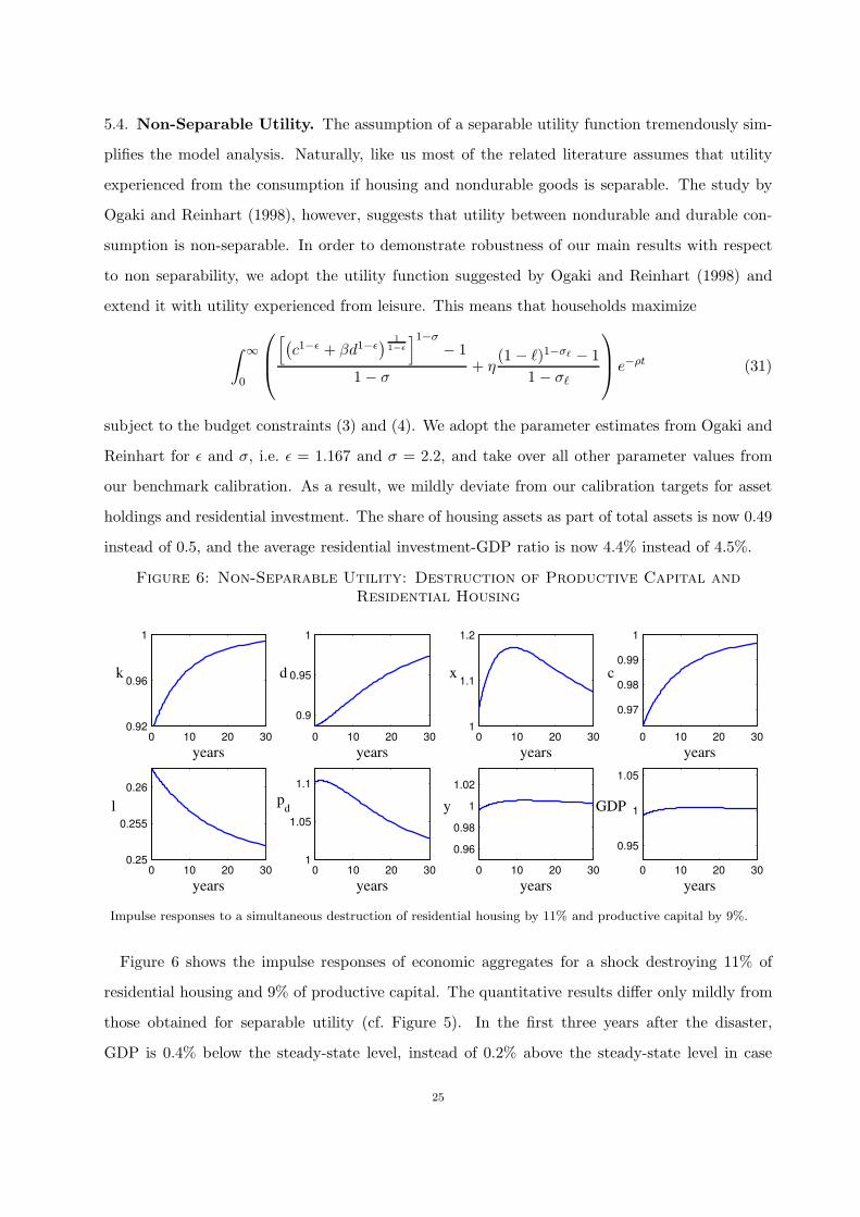
5.4. Non-Separable Utility. The assumption of a separable utility function tremendously sim-
plifies the model analysis. Naturally, like us most of the related literature assumes that utility
experienced from the consumption if housing and nondurable goods is separable. The study by
Ogaki and Reinhart (1998), however, suggests that utility between nondurable and durable con-
sumption is non-separable. In order to demonstrate robustness of our main results with respect
to non separability, we adopt the utility function suggested by Ogaki and Reinhart (1998) and
extend it with utility experienced from leisure. This means that households maximize
∫
∞
0
[
(
c1−ǫ + βd1−ǫ) 1
1−ǫ
]1−σ
− 1
1− σ+ η
(1 − ℓ)1−σℓ − 1
1− σℓ
e−ρt (31)
subject to the budget constraints (3) and (4). We adopt the parameter estimates from Ogaki and
Reinhart for ǫ and σ, i.e. ǫ = 1.167 and σ = 2.2, and take over all other parameter values from
our benchmark calibration. As a result, we mildly deviate from our calibration targets for asset
holdings and residential investment. The share of housing assets as part of total assets is now 0.49
instead of 0.5, and the average residential investment-GDP ratio is now 4.4% instead of 4.5%.
Figure 6: Non-Separable Utility: Destruction of Productive Capital and
Residential Housing
0 10 20 30
0.92
0.96
1
years
k
0 10 20 30
0.9
0.95
1
years
d
0 10 20 30
1
1.1
1.2
years
x
0 10 20 30
0.97
0.98
0.99
1
years
c
0 10 20 30
0.25
0.255
0.26
years
l
0 10 20 30
0.96
0.98
1
1.02
years
y
0 10 20 30
1
1.05
1.1
years
pd
0 10 20 30
0.95
1
1.05
years
GDP
Impulse responses to a simultaneous destruction of residential housing by 11% and productive capital by 9%.
Figure 6 shows the impulse responses of economic aggregates for a shock destroying 11% of
residential housing and 9% of productive capital. The quantitative results differ only mildly from
those obtained for separable utility (cf. Figure 5). In the first three years after the disaster,
GDP is 0.4% below the steady-state level, instead of 0.2% above the steady-state level in case
25
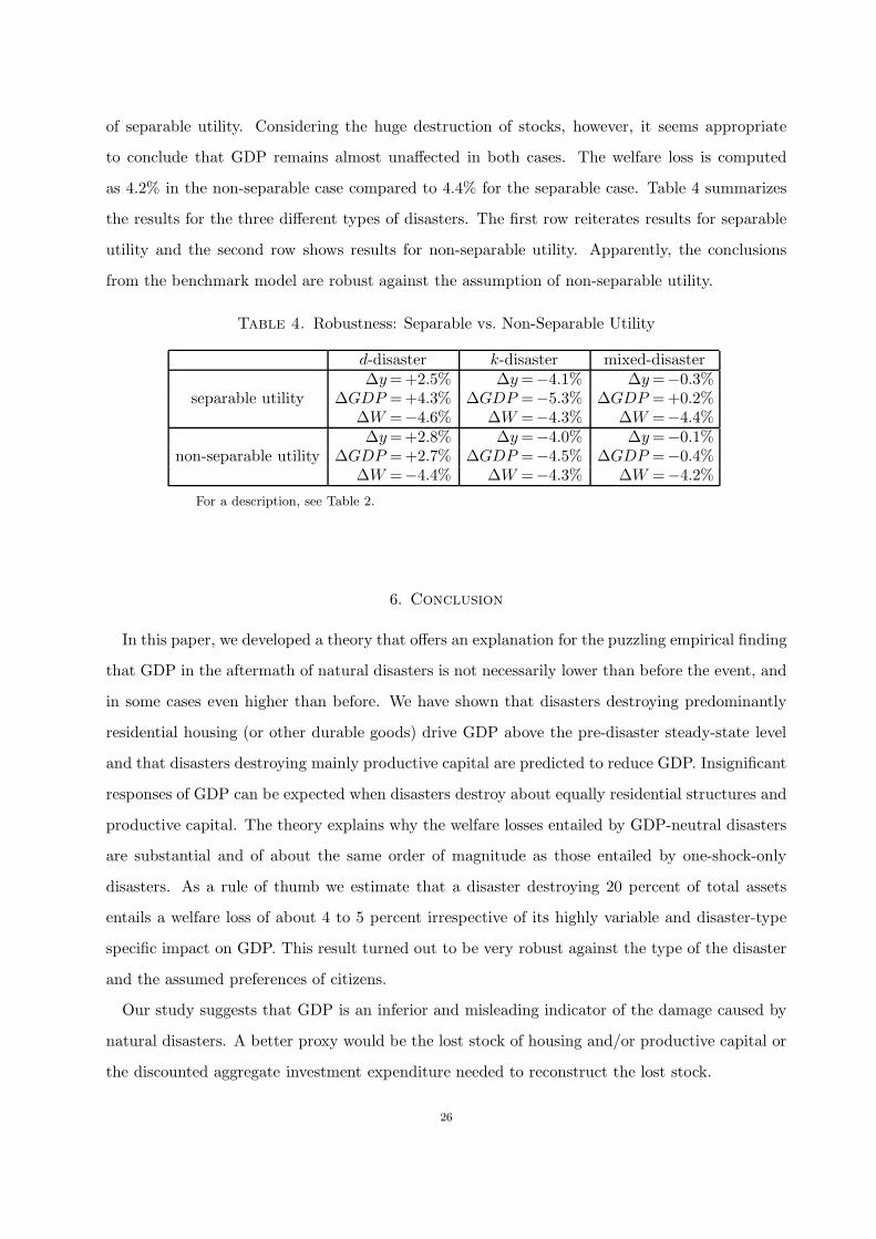
of separable utility. Considering the huge destruction of stocks, however, it seems appropriate
to conclude that GDP remains almost unaffected in both cases. The welfare loss is computed
as 4.2% in the non-separable case compared to 4.4% for the separable case. Table 4 summarizes
the results for the three different types of disasters. The first row reiterates results for separable
utility and the second row shows results for non-separable utility. Apparently, the conclusions
from the benchmark model are robust against the assumption of non-separable utility.
Table 4. Robustness: Separable vs. Non-Separable Utility
d-disaster k-disaster mixed-disaster
separable utility∆y=+2.5% ∆y=−4.1% ∆y=−0.3%
∆GDP =+4.3% ∆GDP =−5.3% ∆GDP =+0.2%∆W =−4.6% ∆W =−4.3% ∆W =−4.4%
non-separable utility∆y=+2.8% ∆y=−4.0% ∆y=−0.1%
∆GDP =+2.7% ∆GDP =−4.5% ∆GDP =−0.4%∆W =−4.4% ∆W =−4.3% ∆W =−4.2%
For a description, see Table 2.
6. Conclusion
In this paper, we developed a theory that offers an explanation for the puzzling empirical finding
that GDP in the aftermath of natural disasters is not necessarily lower than before the event, and
in some cases even higher than before. We have shown that disasters destroying predominantly
residential housing (or other durable goods) drive GDP above the pre-disaster steady-state level
and that disasters destroying mainly productive capital are predicted to reduce GDP. Insignificant
responses of GDP can be expected when disasters destroy about equally residential structures and
productive capital. The theory explains why the welfare losses entailed by GDP-neutral disasters
are substantial and of about the same order of magnitude as those entailed by one-shock-only
disasters. As a rule of thumb we estimate that a disaster destroying 20 percent of total assets
entails a welfare loss of about 4 to 5 percent irrespective of its highly variable and disaster-type
specific impact on GDP. This result turned out to be very robust against the type of the disaster
and the assumed preferences of citizens.
Our study suggests that GDP is an inferior and misleading indicator of the damage caused by
natural disasters. A better proxy would be the lost stock of housing and/or productive capital or
the discounted aggregate investment expenditure needed to reconstruct the lost stock.
26
Our results are insignificantly influenced by the assumed absolute size of the disaster. This
fact allowed us to focus the quantitative analysis exemplarily on disasters leading to a loss of
20 percent of total assets. For larger or smaller disasters, the estimated welfare loss and – in
case of one shock disasters – the estimated GDP responses vary in proportion with the size of
the disaster. Likewise, we can always find a shock composition implying zero disaster impact on
GDP, irrespective of disaster size. This quantitative outcome is a natural consequence of iso-elastic
utility and an iso-elastic, constant-returns-to-scale production function, the usual ingredients of
quantitative macroeconomics.
For very large shocks, however, it seems reasonable to abandon the constant elasticity assump-
tion. In particular, labor supply is likely to be bounded from above. The work day is limited
by 24 hours and for most occupations, physiological limits are reached far earlier. Humans can-
not sustain a physical activity level (PAL) of more than 2.4 times the basal metabolic rate for
an extended period of time (Westerterp, 2001). For example, activities like ‘loading sacks on a
truck’ and ‘carrying wood’ are associated with PAL values of 6.6 (FAO, 2001), implying that a
worker’s energy needs would be 6.6 times his basal metabolic rate if he were occupied with these
activities for 24 hours. Such a “heavy construction worker” could only manage to exert effort for
2.4 · 24/6.6 = 8.7 hours per day. Less energy consuming activities are, of course, sustainable for
longer hours. In any case, upper limits to daily labor supply would help to explain why large
disasters are more frequently found to exert a negative impact on GDP than small disasters (see
Loayza et al., 2012). Extending our model by physiologically-constrained labor supply, for exam-
ple based on Dalgaard and Strulik (2011), could be a promising task for future research on the
macroeconomic implications of natural disasters.
27
Appendix A
We analyze the phase diagram for subsystem (22) and (23), and show that it has a unique and
saddle-point stable steady-state. To do this, we show that the x = 0 isocline and d = 0 isocline
intersect exactly once in the positive quadrant. Saddle-point dynamics can then be inferred from
the phase diagram.
The d = 0 isocline is given by x = δdd. Hence, it is linear with positive slope δd > 0. The x = 0
isocline is given by
(
1 +ψ(x)
x
)
(r + δd) =v′(d)
u′(c). (32)
Both isoclines intersect in the positive quadrant. To see this, notice that limx→0 ψ(x)/x = 0 and
limx→∞ ψ(x)/x = ∞ because ψ is convex and ψ(0) = 0. Hence, for d→ 0, the right-hand side of
equation (32) converges towards infinity implying that x→ ∞, and for d→ 0 the right-hand side
of equation (32) converges to 0 implying that the x = 0 isocline intersects the d axis at a finite
point. An illustration of both isoclines is shown in Figure 1.
In order to prove that the intersect of the isoclines is unique, we begin by showing that the
slope of the x = 0 isocline is always negative. By implicit differentiation of (32), we obtain
dx
dd=
v′′(d)u′(c)
1x
(
ψ′(x)− ψ(x)x
)
(r + δd)< 0. (33)
The numerator is negative, because v is convex, and the denominator is positive, because the
convexity of ψ together with ψ(0) = 0 implies that ψ′(x) > ψ(x)/x. Together, this implies that
the sign of the derivative is negative. Hence, the slopes of the isoclines have opposite signs and
the intersection point is unique.
The isoclines divide the phase diagram into four areas. Saddle-point stability follows from the
dynamics within these areas: Above the d = 0 isocline, d is positive and below d negative; on the
right-hand side of the x = 0 isocline, x is positive, and on the left-hand side, x is negative.
Appendix B
Here, we present an alternative setup in which households rent housing services from firms. We
show that this setup is equivalent to the model in Section 2. The alternative setup allows us to
derive a rental price for durables, pd.
28
Households solve
maxc,d,ℓ
∫
∞
0(u(c) + v(d) + q(1− ℓ)) · e−ρtdt, (34)
subject to
a = wℓ+ ra− c− pdd , (35)
where pd denotes the price for hiring one unit of a durable consumption good (a house) d for one
unit of time. The first order conditions are
u′(c) = λ (36)
v′(d) = λpd (37)
λw = q′(1− ℓ) (38)
λr = λρ− λ . (39)
We derive an equation for pd by combining equation (36) and (37):
pd =v′(d)
u′(c). (40)
Furthermore, substituting equation (36) into (38) yields equation (11), and differentiating equation
(36) with respect to time and combining with equation (39) yields the Keynes-Ramsey rule (10).
There exists a continuum (0, 1) of firms buying installed units of houses x from construction
firms at price px and renting houses d to households. These firms can best be seen as real estate
firms whose only role is to buy installed houses and rent them to households. Hence, these firms
maximize
π =
∫
∞
0(pdd− pxx) e
−rtdt (41)
s.t. d = x− δd (42)
The first order conditions are
px = ν (43)
pd − νδ = νr − ν (44)
29
with ν denoting the shadow price of one installed unit of d in terms of marginal revenues.
There exists a continuum (0, 1) of construction firms converting final goods into housing. These
firms face adjustment costs ψ(x) for installing x units of housing. Each real estate firm is assumed
to engage one construction firm per unit of time but it can change the contracting party at any
point of time. Free entry into the construction sector implies that firms sell x at unit costs:
px = 1 +ψ(x)
x. (45)
Substituting equation (43) into (45), differentiation with respect to time, and substituting (44)
and (40) yields
x
x=
(
ψ′(x)−ψ(x)
x
)
−1 [(
1 +ψ(x)
x
)
(r + δd)−v′(d)
u′(c)
]
, (46)
which is equal to equation (23). Hence, the alternative setup for households renting durable goods
d from real estate firms is equivalent to the benchmark setup.
Appendix C
We show that the steady-state of the large economy described by system (24) - (28) is unique.
We begin by noticing that the capital-labor ratio is pinned down by equation (26). Second, we
exploit the analysis of subsystem (25) and (27) from Section 3. From the analysis above we know
that a higher steady-state value of c leads to a higher steady-state of x and d. We can express this
insight as a steady-state relationship x = s(c) with s′(·) > 0. This means that by substituting for
x and rearranging equation (24) we obtain
k
(
Af(k, ℓ)
k− δk
)
= c+ s(c) + ψ(s(c)) . (47)
The equation states a positive relationship between k and c at the steady-state.
Next, we show that equation (28) constitutes a negative steady-state relation between k and c,
taking the capital-labor ratio as given. We do this by evaluating the derivative at the steady-state
for a constant capital-labor ratio:
dk
dc
∣
∣
∣
∣
KRR
=dk
dl
∣
∣
∣
∣
KRR
·dl
dc= 1 ·
−u′′(c)u′(c)
q′′(1− ℓ)< 0 . (48)
The overall derivative is negative because u′′(·) < 0, q′′(·) < 0, and u′(·) > 0. Equations (47)
and (28) both imply a steady-state relationship between k and c. Finally, noticing that the slopes
30
of the steady-state equations (28) and (47) are of opposite sign, we conclude uniqueness of the
steady-state.
31
References
Baxter, M., 1996, Are consumer durables important for business cycles?, The Review of Economics
and Statistics 78, 147-1505.
Bernanke, B.S., 1984, Permanent income, liquidity, and expenditure on automobiles: evidence
from panel data, Quarterly Journal of Economics 99(3), 587-614.
Cavallo, E., S. Galiani, I. Noy and J. Pantano, 2013, Catastrophic natural disasters and economic
growth, The Review of Economics and Statistics 95(5), 1549-1561.
Cavallo, E. and I. Noy, 2011, Natural disasters and the economy – a survey, International Review
of Environmental and Resource Economics 5, 63-102.
Carlstrom, C.T. and T.S. Fuerst, 2010, Nominal rigidities, residential investment, and adjustment
costs, Macroeconomic Dynamics 14, 136-148.
Cooper, R.W. and J.C. Haltiwanger, 2006, On the nature of capital adjustment costs, Review of
Economic Studies 73, 611-633.
Crespo Cuaresma, J., J. Hlouskova and M. Obersteiner, 2008, Natural disasters as creative de-
struction? Evidence from developing countries, Economic Inquiry 46(2), 214-226.
Dalgaard, C.-J. and H. Strulik, 2011, A physiological foundation for the nutrition-based efficiency
wage model, Oxford Economic Papers 63, 232-253.
Davis, M.A. and J. Heathcote, 2005, Housing and the business cycle, International Economic
Review 46(3), 751-784.
EC, IMF, OECD, UN &World Bank, 2009, System of National Accounts 2008, European Commis-
sion, International Monetary Fund, Organisation for Economic Co-operation and Development,
United Nations and World Bank, New York.
Eerola, E. and N. Maattanen, 2013, The optimal tax treatment of housing capital in the neoclas-
sical growth model, Journal of Public Economic Theory 15(6), 912-938.
Ewing, B.T., J.B. Kruse and M.A. Thompson, 2009, Twister! Employment responses to the 3
May 1999 Oklahoma City tornado, Applied Economics 41(6), 691-702.
FAO, 2001, Human Energy Requirements, Food and nutrition, Technical Support Series 1, Rome.
Fomby, T., Y. Ikeda, and N.V. Loayza, 2013, The growth aftermath of natural disasters, Journal
of Applied Econometrics 28(3), 412-434.
Galor, O. and D.N. Weil, 2000, Population, technology and growth: From the Malthusian regime
to the demographic transition and beyond, American Economic Review 110, 806–828.
Iacoviello, M., 2005, House prices, borrowing constraints, and monetary policy in the business
cycle, American Economic Review 95(3), 739-764.
32
Iacoviello, M., 2010, Housing in DSGE models: findings and new directions, in Bandt, O. de;
Knetsch, Th.; Penalosa, J.; Zollino, F. (Eds.), Housing Markets in Europe: A Macroeconomic
Perspective, Berlin, Heidelberg: Springer-Verlag, pp. 3-16.
Iacoviello, M. 2011, Housing wealth and consumption, International Encyclopedia of Housing and
Home, Elsevier.
Iacoviello, M., and S. Neri, 2010, Housing market spillovers: evidence from an estimated DSGE
model, American Economic Journal: Macroeconomics, 2(2), 125-64.
Knoll, K., M. Schularick, and T.M. Steger, 2014, No price like home: global house prices, 1870 -
2012, University of Leipzig, mimeo.
Leiter, A.M., H. Oberhofer and P.A. Raschky, 2009, Creative disasters? Flooding effects on capital,
labour and productivity within European firms, Environmental and Resource Economics 43,
333-350.
Loayza, N.V., E. Olaberrıa, J. Rigolini and L. Christiaensen, 2012, Natural disasters and growth:
going beyond the averages, World Development 40(7), 1317-1336.
Noy, I., 2009, The macroeconomic consequences of disasters, Journal of Development Economics
88, 221-231.
Ogaki, M. and C.M. Reinhart, 1998, Measuring intertemporal substitution: the role of durable
goods, Journal of Political Economy 106(5), 1078-1098.
Raddatz, C., 2007, Are external shocks responsible for the instability of output in low-income
countries? Journal of Development Economics 84, 155-187.
Shapiro, M.D., 1986, The dynamic demand for capital and labor Quarterly Journal of Economics
101(3), 513-542.
Skidmore, M., and H. Toya, 2002, Do natural disasters promote long-run growth? Economic
Inquiry 40, 664-687.
Strulik, H. and T. Trimborn, 2012, Laffer strikes again: dynamic scoring of capital taxes, European
Economic Review 56, 1180-1199.
Strulik, H. and T. Trimborn, 2014, A note on variable capital utilization in growth and business
cycle theory, Macroeconomic Dynamics, forthcoming.
Topel, R. and S. Rosen, 1988, Housing investment in the United States, Journal of Political
Economy 96(4), 718-740.
Trimborn, T., K.-J. Koch, and T.M. Steger, 2008, Multi-dimensional transitional dynamics: A
simple numerical procedure, Macroeconomic Dynamics, 12, 1-19.
Trimborn, T., 2013, Solution of continuous-time dynamic models with inequality constraints Eco-
nomics Letters 119, 299-301
Westerterp, K.R., 2001, Pattern and intensity of physical activity, Nature 410, 539.
33