Natural convection flow in a square cavity revisited ...environ.chemeng.ntua.gr/en/Uploads/Doc/Papers/CFD/1994_Natural Convection in square...NATURAL CONVECTION FLOW IN A SQUARE CAVITY

INTERNATIONAL JOURNAL FOR NUMERICAL METHODS IN FLUIDS, VOL. 18, 695-719 (1994)

NATURAL CONVECTION FLOW IN A SQUARE CAVITY REVISITED: LAMINAR AND TURBULENT MODELS WITH

WALL FUNCTIONS

G. BARAKOS AND E. MITSOULIS* Department of Chemical Engineering, University of Ottawa, Ottawa, Ont. KIN 6N5, Canada

AND

D. ASSIMACOPOULOS Section II, Department of Chemical Engineering, National Technical University of Athens, Athens 157-73, Greece

SUMMARY Numerical simulations have been undertaken for the benchmark problem of natural convection flow in a square cavity. The control volume method is used to solve the conservation equations for laminar and turbulent Rows for a series of Rayleigh numbers (Ra) reaching values up to 10". The k--E model has been used for turbulence modelling with and without logarithmic wall functions. Uniform and non-uniform (stretched) grids have been employed with increasing density to guarantee accurate solutions, especially near the walls for high Ra-values. AD1 and SIP solvers are implemented to accelerate convergence. Excellent agreement is obtained with previous numerical solutions, while some discrepancies with others for high Ra-values may be due to a possibly different implementation of the wall functions. Comparisons with experimental data for heat transfer (Nusselt number) clearly demonstrates the limitations of the standard k--E model with logarithmic wall functions, which gives significant overpredictions.

KEY WORDS k--E model Turbulence modelling Natural convection Heat transfer

1. INTRODUCTION

Natural convection flow in enclosures has many thermal engineering applications such as in double-glazed windows, solar collectors, cooling devices for electronic instruments, gas-filled cavities around nuclear reactor cores and building in~ulation.'-~ The problem is also of interest to geophysicists in many naturally occurring situations where fluid motion results from buoyancy forces due to temperature gradient^.^ Furthermore, this problem as depicted in its simplified schematic representation of Figure 1 is a good comparison test for the performance evaluation of both numerical techniques and turbulence models (benchmark p r ~ b l e m ) . ~ - ~

Batchelor' was the first to state the mathematical formulation of the problem and give approximate solutions. Poots4 performed calculations by hand and provided the first solution graphs for isotherms and streamlines inside the cavity. Hellums and Churchills performed

Author to whom correspondence should be addressed.

CCC 0271-209 1/94/070695-25 0 1994 by John Wiley & Sons, Ltd.

Received 4 May 1993 Revised 8 November 1993

696 G. BARAKOS, E. MITSOULIS AND D. ASSIMACOPOULOS

numerical calculations and compared their results with experimental data by Martini and Churchill' for natural convection in a cylinder. Ostrach" performed calculations for high values of Rayleigh number (Ra) but for fluids with high Prandtl number (Pr), while the Grashof number (Gr) was set to unity (Ra = Gr Pr). Wilkes and Churchill" and Gill" gave approximate solutions for the flow at the boundary of the cavity. Elder'3v14 performed calculations using a system of five equations; however, some stability problems arose, so he assumed that the normal gradients of vorticity vanish on the horizontal boundary layer of the cavity. Aziz and Hellums' were apparently the first to perform calculations for both two- and three-dimensional flow of fluid heated from below. The final form of the problem was defined by De Vahl DavisI6 and computational results were presented for Rayleigh numbers up to lo6. Results on heat transfer and the effect of variation in the Prandtl number were also presented.

A detailed study of the laminar solution of the problem (Ra up to lo5) was given by MacGregor and Emery' together with experimental results covering a wide range of Prandtl numbers. Many correlations of Nusselt number (Nu) and Ra concerning experimental results can also be found in this paper. Jaluria and Gebhart18 worked on vertical natural convection flows. Their work revealed the process occurring during the transition from laminar to turbulent flow near a flat vertical plate when the surface heat flux is uniform. The interaction of the velocity and temperature fields during the transition and the effect on Nu were also investigated. Mallinson and De Vahl Davis" presented detailed three-dimensional calculations for laminar flow. The calculations were performed for different values of Prandtl number and aspect ratio of cavity dimensions.

Markatos and Pericleous2' were the first to introduce a turbulence model in their calculations. They performed two-dimensional simulations for Rayleigh numbers up to 10' and presented a complete set of graphs for different values of Ra (Pr = 0.71), including isotherms, streamlines and velocity fields. Correlations between Ra and Nu were also presented and good agreement was found between simulations and experimental data by MacGregor and Emery.' The same turbulence model (k--E) was used by Ozoe et ~ 1 . ~ ' for two-dimensional calculations up to Ra = 10" and for aspect ratio A = 2. Results for the flow field and for heat transfer were presented together with a parametric study of the k--E model constants. Oscillations were encountered for the streamfunction at high Ra.

Henkes et al. 22 performed two-dimensional calculations using various versions of the k--E turbulence model. These versions included the standard k--E and low-Reynolds-number k--E models. Their results reached a steady, non-oscillating state even for high Ra (up to 1014), much the same as Markatos and Pericleous." Simulations were performed for air and water. Results for Nu were also presented. They showed that the low-Reynolds-number k--E model has a non-unique solution for the same value of Ra. A comparison with experimental results for Nu showed the superiority of low-Reynolds-number k--E models. Their work gave a very good definition of the problem and an attempt was made to specify many parameters (geometry, k--E constants, grid discretization) so that results by different researchers are directly comparable.

Fusegi et al. 23924 presented three-dimensional calculations for laminar flow for Ra up to 10". Their graphs revealed the three-dimensional character of the flow. Comparisons were made with two-dimensional simulations and differences were reported for the heat transfer correlation between Nu and Ra.

Other works have also been published concerning experimental and numerical results for cavities with partition^,^.^ basically for laminar flow. Effects such as radiation from the cavity walls and participating medium have also been for low values of Ra. Some experimental studies for high Ra have been presented.26

Since good numerical solutions and experimental data exist in the literature,6-8s20*22 the

NATURAL CONVECTION FLOW IN A SQUARE CAVITY 697

simulation of the flow field in a square cavity has been suggested as a benchmark test.6 It is the purpose of the present paper to rework the problem for laminar and turbulent flow for a wide range of Ra. Turbulence is modelled by the standard k--E model and the effect of the assumed wall functions on heat transfer is investigated. A series of solution graphs will be presented to illustrate the flow and temperature field for different Ra-values. Comparison of the present results with previous experimental and numerical data will also be presented. Finally, conclusions will be drawn about the present state of calculations for this benchmark problem.

2. MATHEMATICAL MODEL

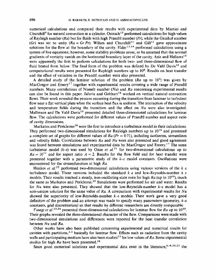
The problem under consideration is depicted schematically in Figure 1. The flow domain is the interior of a 2D square cavity (aspect ratio A = 1) of width W The horizontal walls of the cavity are assumed to be perfectly adiabatic (q = 0), while the vertical walls are kept isothermal with the left wall at high temperature TH and the right wall at low temperature T,. The interior of the cavity is filled with air and all properties are calculated at a reference temperature T,. Owing to heat transfer through the vertical walls, density changes result in a recirculating flow. An increasing Ra causes a pass from a laminar to a turbulent flow state. According to Elder,13 the flow becomes turbulent at Ra greater than lo6; however, according to the present numerical calculations, this transition point depends on the formulation of the turbulence model. Keeping a temperature difference of 20 K between the vertical walls of the cavity and establishing the reference temperature T, at 293 K, an overheat ratio 6 = (TH - T,)/T, = 0.068 is obtained. For this reference temperature and assuming air as the working fluid, the value of Pr equals 0.71 and is kept constant in all the calculations. The small value of 6 allows the use of the Boussinesq approximation for the fluid. In order to obtain a higher Ra, the cavity dimensions were increased while keeping the same temperature difference AT. Table I shows the significant increase in cavity width as Ra goes from lo3 to 1 o ' O .

Figure 1. Schematic representation of cavity problem for natural convection flow along with relevant notation and boundary conditions


Table I. Cavity widths used in calculations

~~~ ~ ~ ~

1 0 3 7.81 x 10-3 1 0 7 1.68 x 10-1

1 0 5 3.63 x 109 7.81 x 10-1 lo4 1.68 x 10' 3.36 x lo-'

lo6 7.81 x 10" 1.68

The Reynolds equations for a Boussinesq incompressible fluid under steady state conditions in a two-dimensional geometry take the

au au

ax ay -+ -=o ,

au au

u - + u - =

while the energy equation becomes

(3)

In the above equations all Reynolds stresses are incorporated into the diffusion terms using a turbulent viscosity v, given by

v, = c, k2/&, (4)

where c, is a constant and k and E are calculated from their transport equations

The two terms Pk and Gk appearing above correspond to the shear and buoyancy production rates of the turbulent kinetic energy respectively and are given by

The values for all constants appearing in the transport equations for k and E are summarized


Table 11. Constants used in k-E turbulence model

CP 0.09 UT 1 .o C l , 1.44 uk 1 .o C 2 r 1.92 ue 1.3

in Table 11. As far as the constant cJa is concerned, the expression suggested by Henkes et al. 22

is used:

U cgE = tanh I I .

The values for u, u, ?; k and E next to the walls are calculated using the wall functions

T + = 2.195 ln(9y') + 13.2Pr - 5.66,

Y+ = YUT/V,

u + = u/u,,

The above wall functions are valid for forced convection flow with small pressure gradients and for y + > 11.5. Other wall functions have also appeared recently in the l i t e r a t ~ r e . ~ ~ - ~ l An alternative is to use wall functions only for k and E ~ ~ * ~ ~ at the first computational grid point after the wall. In this work both modelling techniques will be tested, i.e. use of logarithmic wall functions for all variables (u, o, 7: k, E ) or for k- and &-values alone. Much of the success enjoyed in the prediction of wall-bounded shear flows has depended upon the application of wall f ~ n c t i o n s ~ ~ - ~ ' that relate surface boundary conditions to points in the fluid away from boundaries. The above logarithmic wall functions are checked here for natural convection flows. The case of not using wall functions at all for all variables is not desirable, since it is computationally very intensive for resolving adequately the very thin boundary layers.

700 G . BARAKOS, E. MITSOULIS AND D. ASSIMACOPOULOS

Apart from the turbulence model and the constants appearing in it, the relevant independent dimensionless parameters of the mathematical model are

A = H J W , (19)

P r = V J U , (20)

Ra = g / lATH3PrJv2 . (21)

3. NUMERICAL SCHEME A N D METHOD OF SOLUTION

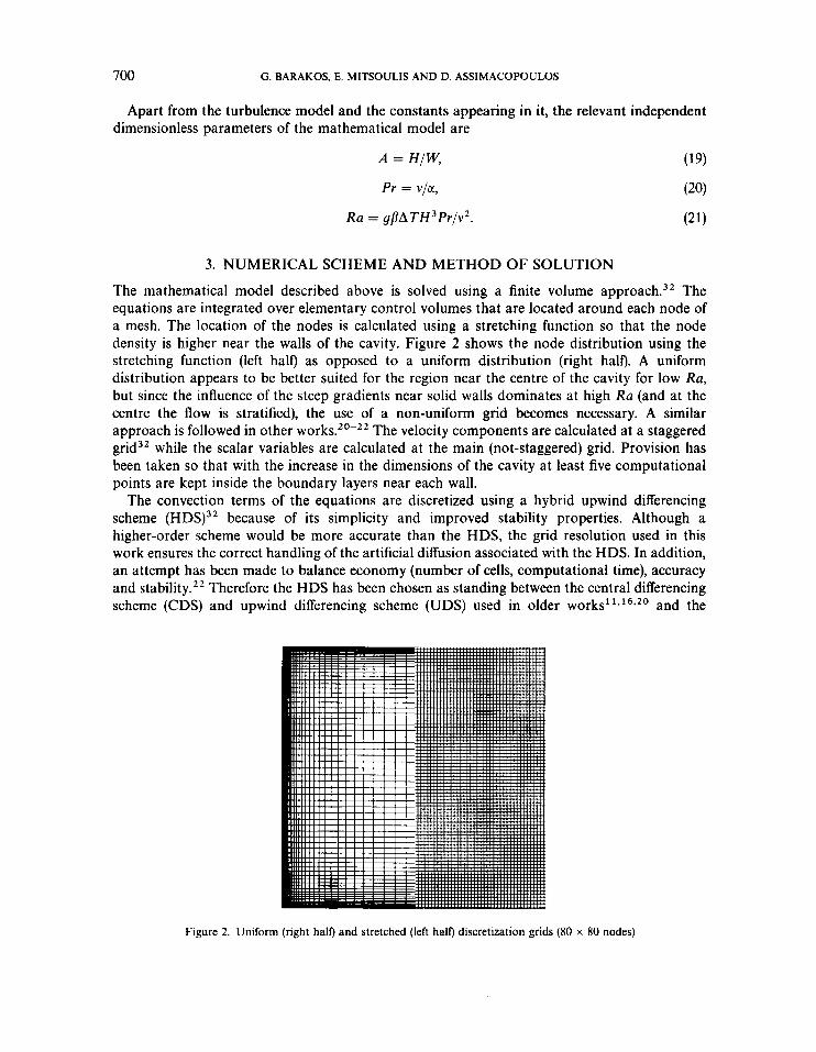
The mathematical model described above is solved using a finite volume approach.32 The equations are integrated over elementary control volumes that are located around each node of a mesh. The location of the nodes is calculated using a stretching function so that the node density is higher near the walls of the cavity. Figure 2 shows the node distribution using the stretching function (left half) as opposed to a uniform distribution (right half). A uniform distribution appears to be better suited for the region near the centre of the cavity for low Ra, but since the influence of the steep gradients near solid walls dominates at high R a (and at the centre the flow is stratified), the use of a non-uniform grid becomes necessary. A similar approach is followed in other works.20-22 The velocity components are calculated at a staggered grid32 while the scalar variables are calculated at the main (not-staggered) grid. Provision has been taken so that with the increase in the dimensions of the cavity at least five computational points are kept inside the boundary layers near each wall.

The convection terms of the equations are discretized using a hybrid upwind differencing scheme (HDS)32 because of its simplicity and improved stability properties. Although a higher-order scheme would be more accurate than the HDS, the grid resolution used in this work ensures the correct handling of the artificial diffusion associated with the HDS. In addition, an attempt has been made to balance economy (number of cells, computational time), accuracy and stability.22 Therefore the HDS has been chosen as standing between the central differencing scheme (CDS) and upwind differencing scheme (UDS) used in older works".'6*20 and the

Figure 2. Uniform (right half) and stretched (left half) discretization grids (80 x 80 nodes)

NATURAL CONVECTION FLOW IN A SQUARE CAVITY 70 1

QUICK scheme used in more recent ones.23v24 The SIMPLEC33 method is used to solve for the pressure, because it was shown to have an improved behaviour over SIMPLE34 as far as stability and convergence speed of the numerical scheme are concerned.

Owing to the density of the grid and the requirement for fast convergence, a mixed technique was used for the solution of the final algebraic equations, in which both alternating direction implicit (ADI) and strongly implicit (SIP) methods35 are used. For each Ra the calculations were started using as initial field values the results of a previous Ra solution. The system of algebraic equations was initially solved by a line-by-line (LBL) solver with ADI. After a number of iterations, switching to SIP was used to accelerate convergence. This technique was found to be extremely useful, especially for calculations at high Ra with the turbulence model.

The convergence criterion used was that the sum of the balance errors over all volumes should be less than

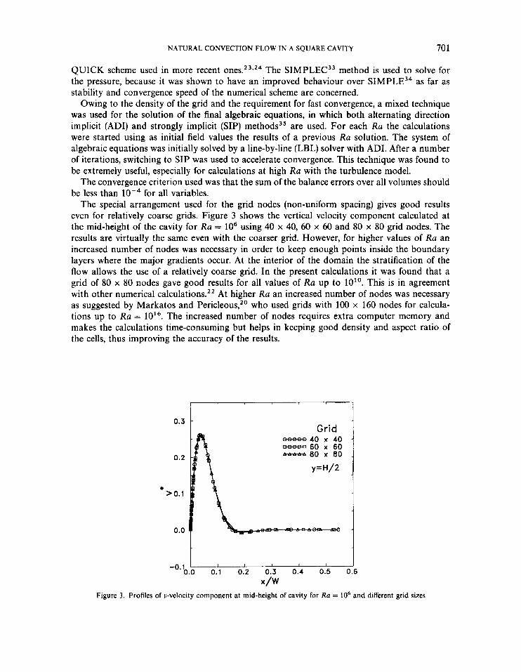
The special arrangement used for the grid nodes (non-uniform spacing) gives good results even for relatively coarse grids. Figure 3 shows the vertical velocity component calculated at the mid-height of the cavity for Ra = lo6 using 40 x 40, 60 x 60 and 80 x 80 grid nodes. The results are virtually the same even with the coarser grid. However, for higher values of Ra an increased number of nodes was necessary in order to keep enough points inside the boundary layers where the major gradients occur. At the interior of the domain the stratification of the flow allows the use of a relatively coarse grid. In the present calculations it was found that a grid of 80 x 80 nodes gave good results for all values of Ra up to 10". This is in agreement with other numerical calculations." At higher Ra an increased number of nodes was necessary as suggested by Markatos and Pericleous,20 who used grids with 100 x 160 nodes for calculations up to Ra = The increased number of nodes requires extra computer memory and makes the calculations time-consuming but helps in keeping good density and aspect ratio of the cells, thus improving the accuracy of the results.

for all variables.

0.3

0.2

>0.1

0.0

1 Grid

meeo 40 x 40 - 60 x 60 - 80 x 80

I

I$ 1 y=H/2

t -0.1 ' I I I I

0.0 0.1 0.2 0.3 0.4 0.5 C 3

Figure 3. Profiles of v-velocity component at mid-height of cavity for Ra = lo6 and different grid sizes

702 G. BARAKOS, E. MlTSOULlS AND D. ASSIMACOPOULOS

4. RESULTS AND DISCUSSION

4.1. Convergence of solution

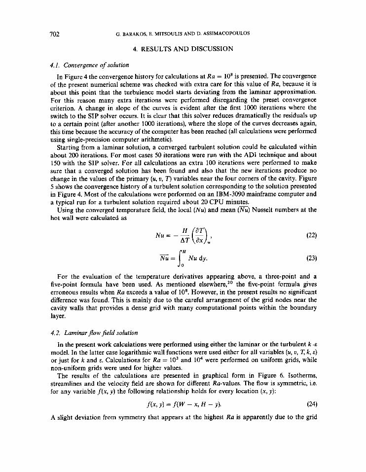
In Figure 4 the convergence history for calculations at Ra = 10' is presented. The convergence of the present numerical scheme was checked with extra care for this value of Ra, because it is about this point that the turbulence model starts deviating from the laminar approximation. For this reason many extra iterations were performed disregarding the preset convergence criterion. A change in slope of the curves is evident after the first 1000 iterations where the switch to the SIP solver occurs. It is clear that this solver reduces dramatically the residuals up to a certain point (after another 1000 iterations), where the slope of the curves decreases again, this time because the accuracy of the computer has been reached (all calculations were performed using single-precision computer arithmetic).

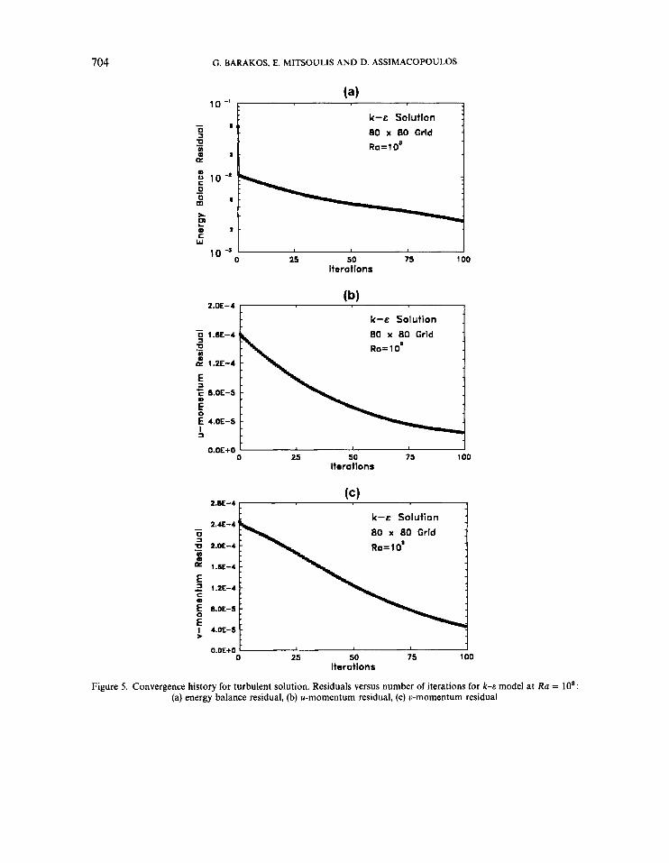
Starting from a laminar solution, a converged turbulent solution could be calculated within about 200 iterations. For most cases 50 iterations were run with the AD1 technique and about 150 with the SIP solver. For all calculations an extra 100 iterations were performed to make sure that a converged solution has been found and also that the new iterations produce no change in the values of the primary (u, u, T) variables near the four corners of the cavity. Figure 5 shows the convergence history of a turbulent solution corresponding to the solution presented in Figure 4. Most of the calculations were performed on an IBM-3090 mainframe computer and a typical run for a turbulent solution required about 20 CPU minutes.

Using the converged temperature field, the local (Nu) and mean (Nu) Nusselt numbers at the hot wall were calculated as

- Nu = loH Nu dy.

For the evaluation of the temperature derivatives appearing above, a three-point and a five-point formula have been used. As mentioned elsewhere,20 the five-point formula gives erroneous results when Ra exceeds a value of 10'. However, in the present results no significant difference was found. This is mainly due to the careful arrangement of the grid nodes near the cavity walls that provides a dense grid with many computational points within the boundary layer.

4.2. Laminar flow field solution

In the present work calculations were performed using either the laminar or the turbulent k-E model. In the latter case logarithmic wall functions were used either for all variables (u, v, IT; k, E ) or just for k and E. Calculations for Ra = lo3 and lo4 were performed on uniform grids, while non-uniform grids were used for higher values.

The results of the calculations are presented in graphical form in Figure 6. Isotherms, streamlines and the velocity field are shown for different Ra-values. The flow is symmetric, i.e. for any variable f ( x , y) the following relationship holds for every location (x, y):

f ( x , Y) = fW - x, H - Y). (24)

A slight deviation from symmetry that appears at the highest Ra is apparently due to the grid

NATURAL CONVECTION FLOW IN A SQUARE CAVITY

(4 l b ' t ' ' - ' . , , . - i

703

- 0 a 3 : 1b* a C - lQS

1 Lominor Solution 1 80 x 80 Grld

0 two 2000 I#K) 4000 SO00 Iterations

Lamlnor Solution 80 x 80 Grld

lo00 2o00 sow 4000 ~W ltsratlons

I > 1cr7

(c)

Laminar Solutlon 80 x 80 Grld

0 1000 2000 3000 4mo so00 ltsrotlons

(c)

Laminar Solutlon 80 x 80 Grld

0 1000 2000 3000 4mo so00 ltsrotlons

Figure 4. Convergence history for laminar solution. Residuals versus number of iterations at Ra = 10': (a) energy balance residual, (b) u-momentum residual, (c) o-momentum residual

704 G . BARAKOS, E. MlTSOULlS AND D. ASSIMACOPOULOS

k--E Solution 1 80 x 80 Grld m Ra=108 Q

wl 10 J 0 25 50 75 100

Iterations

(b) 2.OE-4 -

k--E Solution 80 x 80 Grid

O.OE+O 0 25 50 75 100

iterations

k--E Solution

80 x 80 Grid

> , O.OE+O 1

0 25 50 75 100 Iterations

Figure 5. Convergence history for turbulent solution. Residuals versus number of iterations for k--E model at Ra = 10': (a) energy balance residual, (b) u-momentum residual, (c) u-momentum residual


(a)

705

L

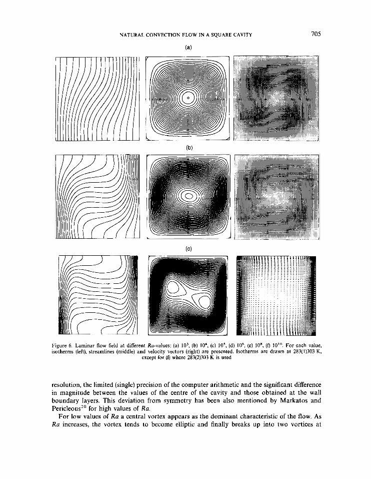
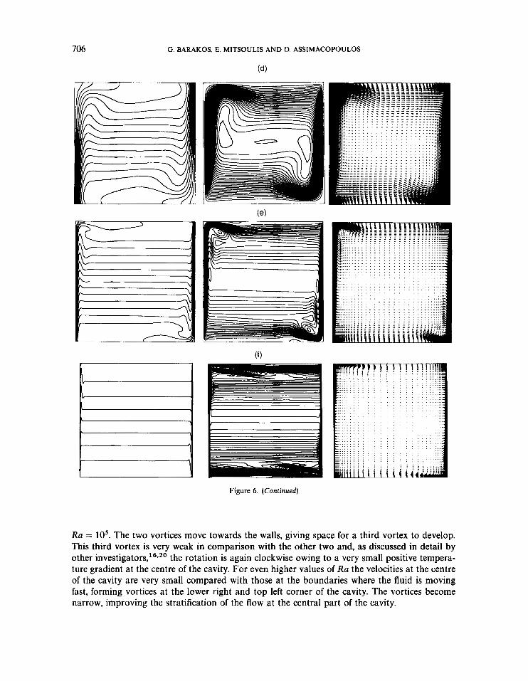
Figure 6. Laminar flow field at different Ra-values: (a) lo3, (b) lo4, (c) lo5, (d) lo6, (e) lo8, (f) 10". For each value, isotherms (left), streamlines (middle) and velocity vectors (right) are presented. Isotherms are drawn at 283(1)303 K,

except for (f) where 283(2)303 K is used

resolution, the limited (single) precision of the computer arithmetic and the significant difference in magnitude between the values of the centre of the cavity and those obtained at the wall boundary layers. This deviation from symmetry has been also mentioned by Markatos and Pericleous'' for high values of Ra.

For low values of Ra a central vortex appears as the dominant characteristic of the flow. As Ra increases, the vortex tends to become elliptic and finally breaks up into two vortices at


(d)

Figure 6. (Continued)

Ra = lo5. The two vortices move towards the walls, giving space for a third vortex to develop. This third vortex is very weak in comparison with the other two and, as discussed in detail by other the rotation is again clockwise owing to a very small positive temperature gradient at the centre of the cavity. For even higher values of Ra the velocities at the centre of the cavity are very small compared with those at the boundaries where the fluid is moving fast, forming vortices at the lower right and top left corner of the cavity. The vortices become narrow, improving the stratification of the flow at the central part of the cavity.


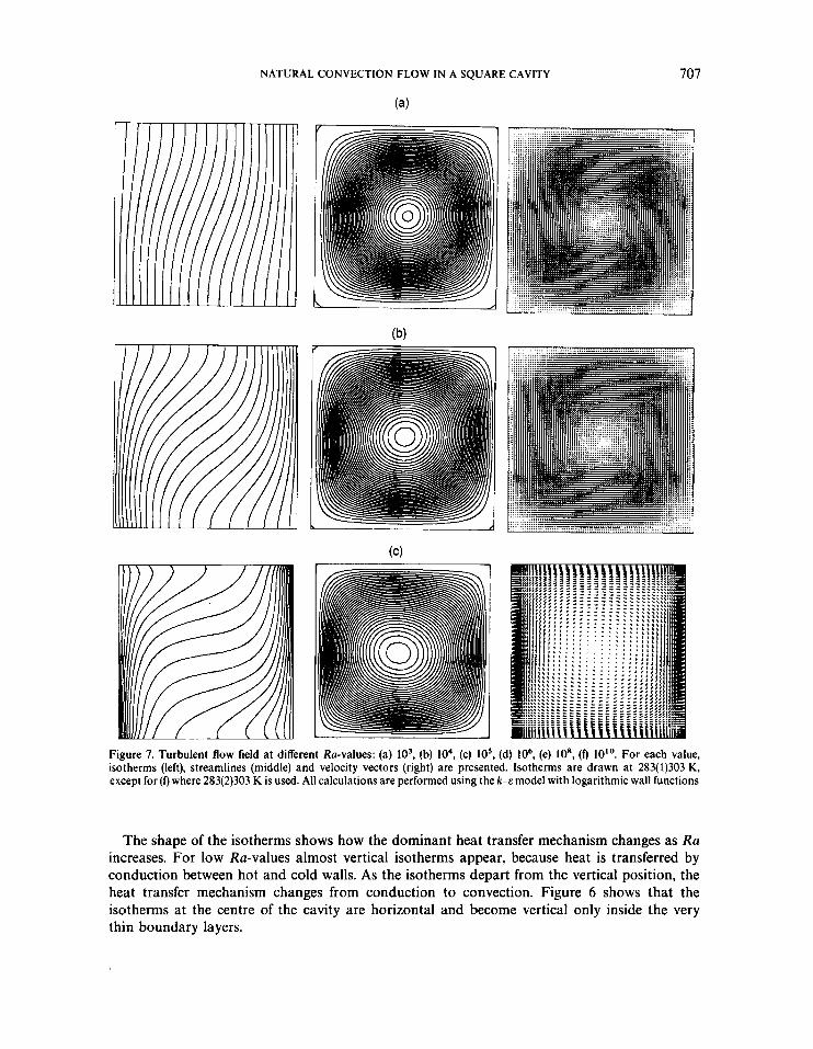
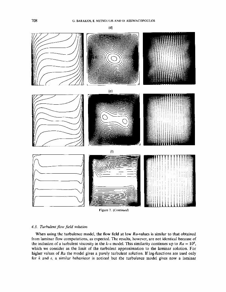
Figure 7. Turbulent flow field at different Ra-values: (a) lo3, (b) lo4, (c) los, (d) lo6, (e) lo8, (0 loLo. For each value, isotherms (left), streamlines (middle) and velocity vectors (right) are presented. Isotherms are drawn at 283( 1)303 K, except for ( f ) where 283(2)303 K is used. All calculations are performed using the k--E model with logarithmic wall functions

The shape of the isotherms shows how the dominant heat transfer mechanism changes as Ra increases. For low Ra-values almost vertical isotherms appear, because heat is transferred by conduction between hot and cold walls. As the isotherms depart from the vertical position, the heat transfer mechanism changes from conduction to convection. Figure 6 shows that the isotherms at the centre of the cavity are horizontal and become vertical only inside the very thin boundary layers.


(4

. . . . . . . . . . . . . .

, . . . . . . . .

. . . . . . . . . . . . .

Figure 7. (Continued)

4.3. Turbulent flow field solution

When using the turbulence model, the flow field at low Ra-values is similar to that obtained from laminar flow computations, as expected. The results, however, are not identical because of the inclusion of a turbulent viscosity in the k--E model. This similarity continues up to Ra = lo6, which we consider as the limit of the turbulent approximation to the laminar solution. For higher values of Ra the model gives a purely turbulent solution. If log-functions are used only for k and E, a similar behaviour is noticed but the turbulence model gives now a laminar


' -O B

1 .o

0.8

0.6

I-

0.4

0.2

0.8

0.6 . I-

0.4

0.2

0.0 0.0 0.2 0.4 0.6 0.8 1 .o

x/w

(b)

Ra - 10' - 10' - 10' - 10' - 10' - 10' - 10'0

0 . 0 ' " " " " ' 0.0 0.2 0.4 0.6 0.8 1

x/w

I I D

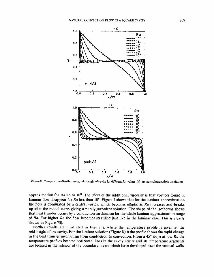
Figure 8. Temperature distribution at mid-height of cavity for different Ra-values: (a) laminar solution, (b) k--E solution

approximation for Ra up to 10'. The effect of the additional viscosity is that vortices found in laminar flow disappear for Ra less than lo*. Figure 7 shows that for the laminar approximation the flow is dominated by a central vortex, which becomes elliptic as Ra increases and breaks up after the model starts giving a purely turbulent solution. The shape of the isotherms shows that heat transfer occurs by a conduction mechanism for the whole laminar approximation range of Ra. For higher Ra the flow becomes stratified just like in the laminar case. This is clearly shown in Figure 7(f).

Further results are illustrated in Figure 8, where the temperature profile is given at the mid-height of the cavity. For the laminar solution (Figure 8(a)) the profile shows the rapid change in the heat transfer mechanism from conduction to convection. From a 45" slope at low Ra the temperature profiles become horizontal lines in the cavity centre and all temperature gradients are located in the interior of the boundary layers which have developed near the vertical walls.

710 G. BARAKOS. E. MITSOULIS AND D. ASSIMACOPOULOS

U

I 2

-0.4 -0.2 0.0. 0.2 u

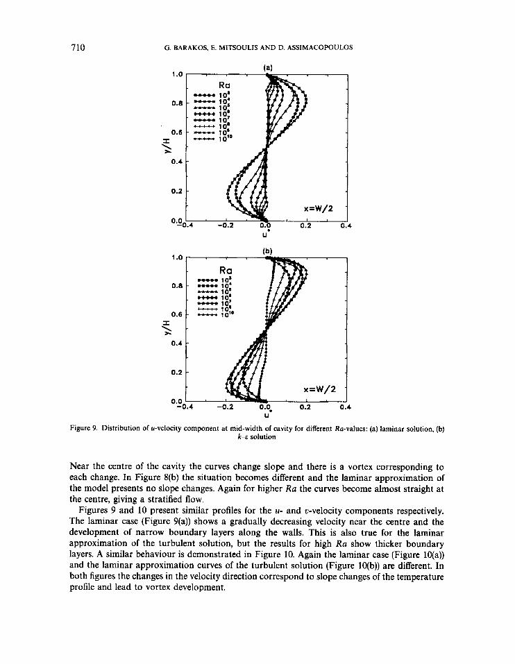
Figure 9. Distribution of u-velocity component at mid-width of cavity for different Ra-values: (a) laminar solution, (b) k--E solution

Near the centre of the cavity the curves change slope and there is a vortex corresponding to each change. In Figure 8(b) the situation becomes different and the laminar approximation of the model presents no slope changes. Again for higher Ra the curves become almost straight at the centre, giving a stratified flow.

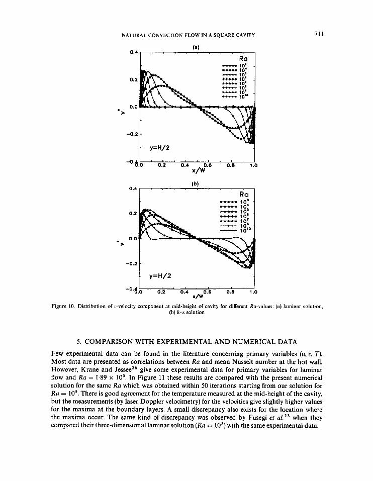
Figures 9 and 10 present similar profiles for the u- and u-velocity components respectively. The laminar case (Figure 9(a)) shows a gradually decreasing velocity near the centre and the development of narrow boundary layers along the walls. This is also true for the laminar approximation of the turbulent solution, but the results for high Ra show thicker boundary layers. A similar behaviour is demonstrated in Figure 10. Again the laminar case (Figure lqa)) and the laminar approximation curves of the turbulent solution (Figure 10(b)) are different. In both figures the changes in the velocity direction correspond to slope changes of the temperature profile and lead to vortex development.


(4 0.4

Ra - loa

- y=H/2

0 >

0.2

0.0

-0.2

- lo4 - 10: - 10 - 10' - 1o'O

-o'd.b 0:2! ' 0.i * ' ' 0.8 ' ' 1.0 ' - (b)

0.4 Ra - los - lo4 - los - 10' - 10'

71 1

Figure 10. Distribution of u-velocity component at mid-height of cavity for different Ra-values: (a) laminar solution, (b) k--E solution

5. COMPARISON WITH EXPERIMENTAL AND NUMERICAL DATA

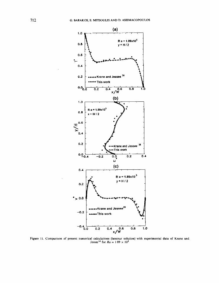
Few experimental data can be found in the literature concerning primary variables (u, u, T). Most data are presented as correlations between Ra and mean Nusselt number at the hot wall. However, Krane and J e ~ s e e ~ ~ give some experimental data for primary variables for laminar flow and Ra = 1.89 x lo5. In Figure 11 these results are compared with the present numerical solution for the same Ra which was obtained within 50 iterations starting from our solution for Ra = lo5. There is good agreement for the temperature measured at the mid-height of the cavity, but the measurements (by laser Doppler velocimetry) for the velocities give slightly higher values for the maxima at the boundary layers. A small discrepancy also exists for the location where the maxima occur. The same kind of discrepancy was observed by Fusegi et when they compared their three-dimensional laminar solution (Ra = lo5) with the same experimental data.

712

1 .o

Oo8

0.6 I

0.4 2 -

0.2

0.0

G. BARAKOS. E. MITSOULIS AND D. ASSIMACOPOULOS

R a = 1 .89~10~ - x = w / 2

-

-

-

1 .o

0.6

0.6

I-

0.4

(a)

R a = 1 .89x105 y = H 1 2

0

...am Krane and J e ~ s e e ~ ~

0.8 1.0 OS4 ./i.6 0.0 0.2

Figure 11. Comparison of present numerical calculations (laminar solution) with experimental data of Krane and J e ~ s e e ’ ~ for Ra = 1.89 x lo5

NATURAL CONVECTION FLOW JN A SQUARE CAVITY 713

Table 111. Comparison of laminar solution with previous works for different Ra-values

This work Markatos and Pericleous2’ De Vahl Davis6 Fusegi et

Ra = lo3

N u m e a n 1.1 14 1.108 Numax (at y / H ) 1.581 (0.099) 1.596 (0.083) Numi, (at y / H ) 0.670 (0.994) 0.720 (0.993) %a, (at Y l H ) 0,153 (0.806) (0.832) urnax (at x / W 0.155 (0.181) (0.168)

~ ~~~

1.118 1.105 1.505 (0.092) 1.420 (0.083) 0.692 (1.000) 0.764 (1.000) 0.1 36 (0.8 13) 0.132 (0.833) 0.138 (0.178) 0.131 (0.200)

N % e a n 2.245 2.201 Nu,,, (at y / H ) 3.539 (0.143) 3.482 (0.143) Numi, (at y / H ) 0.583 (0.994) 0.643 (0.993) ~ m a x (at Y / H ) 0-193 (0.818) (0.832) ~ m a x (at x / w 0.234 (0.1 19) (0.1 13)

2.243 2.302 3.528 (0.143) 3.652 (0.623) 0.586 (1.000) 0.61 1 (1~OOO) 0.192 (0.823) 0.20 1 (0.8 17) 0.234 (0.1 19) 0.225 (0.1 17)

Ra = lo5

N u m e a n 4.510 4.430 Nu,,, (at y / H ) 7.636 (0.085) 7.626 (0.083) Numi, (at y / H ) 0.773 (0.999) 0.824 (0.993) urnax (at Y / H ) 0,132 (0.859) (0.857) urn,, (at X/W) 0.258 (0.066) (0.067)

4.519 4.646 7.717 (0.081) 7.795 (0.083) 0.729 ( 1 .OW) 0.787 (1.000) 0.153 (0.855) 0.147 (0.855) 0.261 (0.066) 0.247 (0.065)

Ra = lo6

N u m e a n 8.806 8.754 Nu,,, (at y / H ) 17.442 (0.0368) 17.872 (0.0375) Numi, (at y / H ) 1.001 (0.999) 1.232 (0.993) urnax (at Y / H ) 0.077 (0.859) (0.872) oms. (at x /W) 0.262 (0.039) (0.038)

8.799 9.012 17.925 (0.0378) 17.670 (0.0379) 0.989 (1.000) 1.257 (1,000) 0.079 (0.850) 0.084 (0.856) 0.262 (0.038) 0.259 (0.033)

In Table 111 a comparison is given between the present laminar solution and numerical results found in the The comparison concerns the mean. N u along the hot wall, its maximum and minimum values and the locations where they occur. The same is also done for the maximum and minimum velocity values and their corresponding locations. There is excellent agreement between the present results and the benchmark solution by De Vahl Davis6 for all values of Ra, as well as with the solutions by Markatos and P e r i c l e o ~ s ~ ~ and Fusegi et ul.23*24 All four solutions are less than 7% apart.

Laminar solution data at higher Ra are more difficult to find. Therefore a comparison is only made with the solution by Henkes et al.” for the mean N u along the hot wall in Table IV. Again excellent agreement is found between the two solutions. The maximum difference is 3 5 % for Ra = 10”. For the turbulent case Table V presents a comparison of our results for the mean Nu with results by Markatos and Pericleous” and Henkes et ~ 1 . ~ ’ For Ra = lo8 the three solutions agree remarkably well. As Ra increases, our results without log-functions show excellent agreement with the solution by Henkes et al.,” while Markatos and Pericleous” give somewhat higher values. Introduction of wall functions in the present work gave higher values for the mean N u than those obtained by Markatos and Pericleous.” Obviously a different formulation for the log-functions employed by the latter must be responsible for this disagreement.

714 G . BARAKOS, E. MITSOULIS AND D. ASSIMACOPOULOS

Table IV. Comparison of laminar solution with previous work (mean Nu at high Ra-values)

This work 30.1 54.4 97.6 165.1 Henkes et a1." 30.4 54.1 - 171.0

Table V. Comparison of turbulent solution with previous works (mean Nu at high Ra-values)

Ra 108 109 1010

This work (no wall functions) 32.3 60.1 134.6 Henkes et a1." 32.5 59.5 133.4 Markatos and Pericleous" 32.05 74.7 156.85

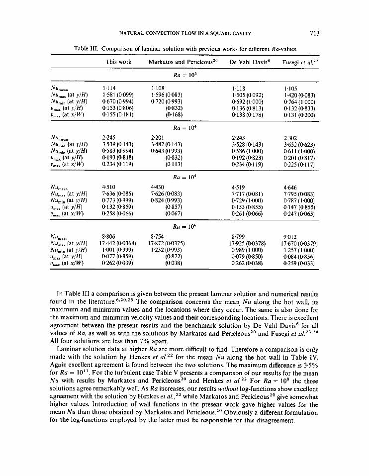
Figure 12 shows a comparison between the three solutions. The present results show that the turbulence formulation with logarithmic wall functions deviates from the laminar approximation solution at Ra x lo6 and gives higher predictions for Nu. The turbulence formulation without logarithmic wall functions approaches the laminar solution up to Ra x 10' and then deviates, giving a turbulent solution. Our results, as well as the results by Henkes er ~ 1 . ~ ~ and Markatos and Pericleous," show that the turbulent solution starts deviating from the laminar approxima-

I U w 3 Z

0.1 6

0.14

0.1 2

0.10 I * Henkes et 0 1 . 1 - Henkes et 0 1 . ~ '

0.08

0.06

0.04 I I I I

0.02 - 11111111 '"""d ' l l l l ld '""" '1 ' - '"""'1 ' ' 1 " " 1 ' ' 1 ' ' ' ' ' ' ' ''"''d - 1 0 1 0 10 1 0 1 0 1 0 * loo 1 0 loio l 1 1 0 " 1 0 lJio 1410 lS

Ra Figure 12. Mean Nusselt number (%) calculated at hot wall as a function of Ra. The straight line corresponds to the

semi-analytical estimate given by Henkes er aLz2


tion around this Ru-value. In the same figure the semi-analytical estimation (straight line) for Nu-Ru-1 /3 provided by Henkes et ~ 1 . ~ ~ is also presented. It is clear that abandoning the wall functions brings our results towards the right direction.

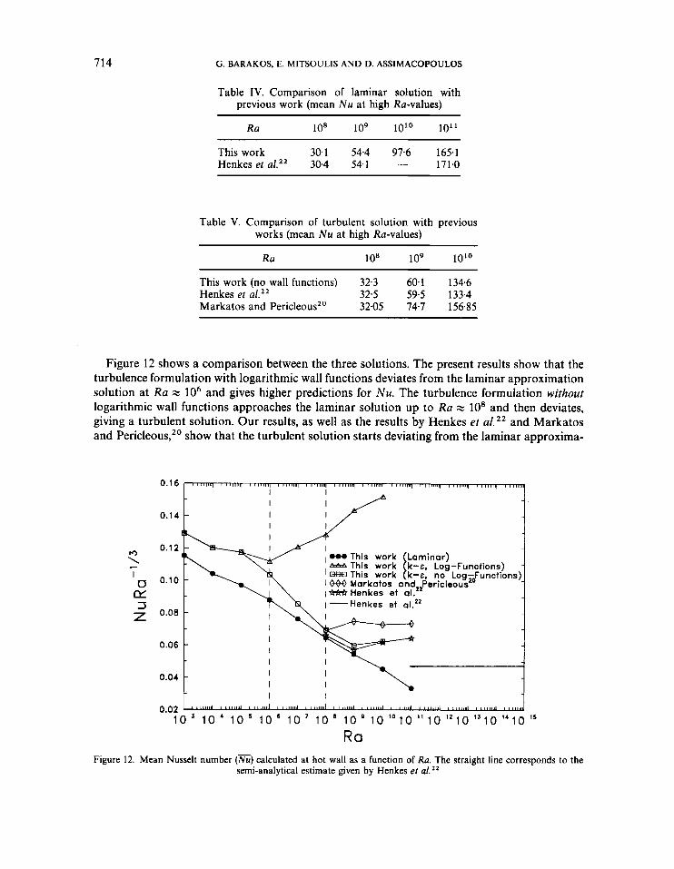
A more dramatic manifestation of the differences between laminar and turbulent (with wall functions) solutions is given in Figure 13, where the Nu-profile is plotted along the hot wall. There is a significant change in shape and magnitude as the k-e model departs from the laminar approximation.

0 N u

Figure 13. Laminar and turbulent Nu at hot wall for different Ra-values (k-c results including logarithmic wall functions)

- A-H-A-A This work Laminar) - WH-0 This work

- ***** Henkes et 0 1 . ’ ~ [k-E)

t -I- c $ c >.

k-f , no Log-Functions) * * * * * Henkes et 01.’ Laminar)

> 0

O1.0 - 4-

0

c 0

0 0 +-

.- t

.- ‘0.5 e ts

-

- E L a

Ra

>. c > 0

O1.0

- A-H-A-A This work Laminar) - WH-0 This work

- ***** Henkes et 0 1 . ’ ~ [k-E)

t -I- c $ k-f , no Log-Functions)

* * * * * Henkes et 01.’ Laminar)

A -

4-

0

c 0

0 0 +-

.- t

.- ‘0.5 e ts

-

- E L a

Ra Figure 14. Thermal stratification at cavity centre versus Ra obtained from laminar and turbulent solutions


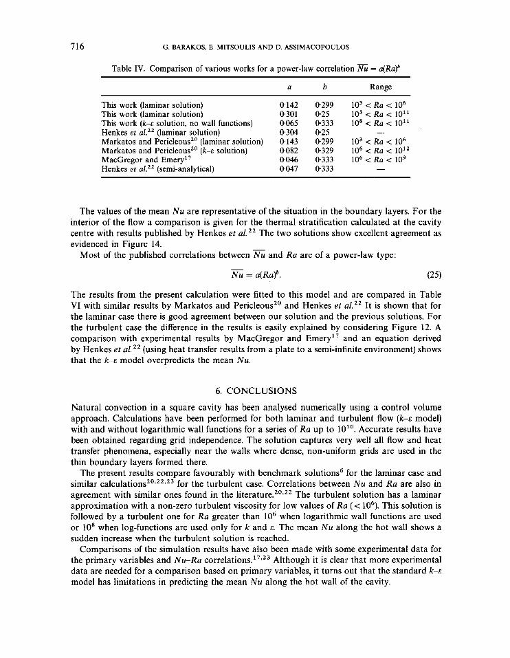
Table IV. Comparison of various works for a power-law correlation Nu = a(Ra)b

a b Range

This work (laminar solution) This work (laminar solution) This work (k--E solution, no wall functions) Henkes et a1.” (laminar solution) Markatos and PericleousZo (laminar solution) Markatos and Pericleous” ( k - ~ solution) MacGregor and Emery” Henkes et aL2’ (semi-analytical)

0.142 0.301 0.065 0.304 0.143 0.082 0.046 0.047

0.299 0.25 0.333 0.25 0.299 0.329 0.333 0.333

lo3 < Ra < lo6 lo3 < Ra < 10” lo8 < Ra < 10”

lo3 < Ra < lo6 lo6 < Ra < 10l2 lo6 < Ra < lo9

-

The values of the mean N u are representative of the situation in the boundary layers. For the interior of the flow a comparison is given for the thermal stratification calculated at the cavity centre with results published by Henkes et al.” The two solutions show excellent agreement as evidenced in Figure 14.

Most of the published correlations between and R a are of a power-law type: - N u = ~ ( R u ) ~

The results from the present calculation were fitted to this model and are compared in Table VI with similar results by Markatos and Pericleous” and Henkes et a1.” It is shown that for the laminar case there is good agreement between our solution and the previous solutions. For the turbulent case the difference in the results is easily explained by considering Figure 12. A comparison with experimental results by MacGregor and Emery’ ’ and an equation derived by Henkes et al. ’’ (using heat transfer results from a plate to a semi-infinite environment) shows that the k--E model overpredicts the mean Nu.

6. CONCLUSIONS

Natural convection in a square cavity has been analysed numerically using a control volume approach. Calculations have been performed for both laminar and turbulent flow (k--E model) with and without logarithmic wall functions for a series of R a up to 10”. Accurate results have been obtained regarding grid independence. The solution captures very well all flow and heat transfer phenomena, especially near the walls where dense, non-uniform grids are used in the thin boundary layers formed there.

The present results compare favourably with benchmark solutions6 for the laminar case and similar calculation^^^^^^^^^ fo r the turbulent case. Correlations between N u and Ra are also in agreement with similar ones found in the literature.20*22 The turbulent solution has a laminar approximation with a non-zero turbulent viscosity for low values of Ra (< lo6). This solution is followed by a turbulent one for R a greater than lo6 when logarithmic wall functions are used or 10’ when log-functions are used only for k and E. The mean N u along the hot wall shows a sudden increase when the turbulent solution is reached.

Comparisons of the simulation results have also been made with some experimental data for the primary variables and Nu-Ra correlations.’ 7 , 2 3 Although it is clear that more experimental data are needed for a comparison based on primary variables, it turns out that the standard k--E model has limitations in predicting the mean N u along the hot wall of the cavity.


Apart from the turbulence model, the use of logarithmic wall functions for the temperature and velocity leads to significant overpredictions for Nu. Since the most important phenomena occur near the cavity walls while the core remains stratified, such an influence is expected. Logarithmic wall functions have been proved inaccurate for predicting heat transfer in natural convection, since by dropping them, a much more reasonable prediction for the heat transfer is obtained. Therefore new types of wall functions such as the power-law ones suggested by George and Capp" for the velocity and temperature in combination with modified versions of the k-E model for low-Reynolds-number flows must be checked.

ACKNOWLEDGEMENTS

Financial support from the Natural Sciences and Engineering Research Council of Canada (NSERC) is gratefully acknowledged.

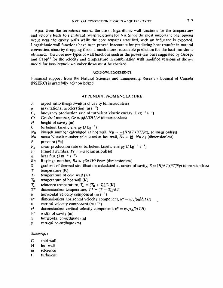
A 9

Gr H k Nu Nu P Pk Pr 4 Ra S T

Gk

-

Tc TH Tm T*

U*

V*

W

Y

U

V

X

APPENDIX: NOMENCLATURE

aspect ratio (height/width) of cavity (dimensionless) gravitational acceleration (m s-') buoyancy production rate of turbulent kinetic energy (J kg-' s - I ) Grashof number, Gr = gPA7H3/vz (dimensionless) height of cavity (m) turbulent kinetic energy (J kg- ') Nusselt number calculated at hot wall, N u = - (H/AT)(aT/ax), (dimensionless) mean Nusselt number calculated at hot wall, 5 = 5:: Nu dy (dimensionless) pressure (Pa) shear production rate of turbulent kinetic energy (J kg-' s-') Prandtl number, Pr = v/a (dimensionless) heat flux (J m-'s-') Rayleigh number, Ra = g ~ A 7 H 3 P r / v 2 (dimensionless) gradient of thermal stratification calculated at centre of cavity, S = (H/AT)(dT/ay) (dimensionless) temperature (K) temperature of cold wall (K) temperature of hot wall (K) reference temperature, T, = (TH + TJ2 (K) dimensionless temperature, T* = (T - T,)/AT horizontal velocity component (m s- ') dimensionless horizontal velocity component, u* = u/J(gPA TH) vertical velocity component (m s - ') dimensionless vertical velocity component, v* = v/J(gBATH) width of cavity (m) horizontal co-ordinate (m) vertical co-ordinate (m)

Subscripts

C cold wall H hot wall m reference t turbulent


Greek letters

coefficient of thermal diffusion (m2 s- *) coefficient of thermal expansion, B = l/Tm (K-I) overheat ratio, S = ( T , - T‘)/Tm (dimensionless) characteristic temperature difference, AT = TH - T, (K) dissipation rate of turbulent kinetic energy (m’ s - ~ ) molecular kinematic viscosity (m’ s- I )

turbulent kinematic viscosity (m’ s-’) density (kg m-3) turbulent Prandtl number for T (dimensionless) turbulent Prandtl number for k (dimensionless) turbulent Prandtl number for E (dimensionless)

REFERENCES

1. G. K. Batchelor, ‘Heat transfer by free convection across a closed cavity between vertical boundaries at different

2. M. Ciofalo and T. G. Karayiannis, ‘Natural convection heat transfer in a partially-or completely-partitioned

3. K. M. Kelkar and S. V. Patankar, ‘Numerical prediction of natural convection in square partitioned enclosures,’

4. G. Poots, ‘Heat transfer by laminar free convection in enclosed plane gas layers,’ Q. Appl. Math., 11,257-273 (1958). 5. J. D. Hellums and S. W. Churchill, ‘Transient and steady state free and natural convection, numerical solutions,’

6. G. De Vahl Davis, ‘Natural convection of air in a square cavity, a bench-mark numerical solution,’ Inr. j. numer.

7. G. De Vahl Davis and I. P. Jones, ‘Natural convection of air in a square cavity: a comparison exercise,’ Inr. j.

8. M. Hortmann, M. Peric and G. Scheuerer, ‘Finite volume multigrid prediction of laminar natural convection:

9. W. R. Martini and S. W. Churchill, ‘Natural convection inside a horizontal cylinder,’ AlChE J., 6,251-257 (1960). 10. J. Ostrach, ‘Completely confined natural convection,’ Developments in Mechanics, Proc. Tenth Midwestern Mechanics

11. J . 0. Wilkes and S. W. Churchill, ‘The finite-difference computation of natural convection in a rectangular enclosure,’

12. A. E. Gill, ‘The boundary-layer regime for convection in a rectangular cavity,’ J. Fluid Mech., 25, 515-536 (1966). 13. J. W. Elder, ‘Turbulent free convection in a vertical slot,’ J. Fluid Mech., 23, 99-111 (1966). 14. J. W. Elder, ‘Numerical experiments with free-convection in a vertical slot,’ J. Fluid Mech., 24, 823-843 (1966). 15. K. Aziz and J. D. Hellums, ‘Numerical solutions of the dimensional equations of motion for laminar natural

16. G. De Vahl Davis, ‘Laminar natural convection in an enclosed rectangular cavity,’ Int. J. Heat Mass Transfer, 11,

17. R. K. MacGregor and A. F. Emery, ‘Free convection through vertical plane layers-moderate and high Prandtl number fluids,’ ASME J. Heat Transfer, 391-403 (August 1969).

18. Y. Jaluria and B. Gebhart, ‘On transition mechanisms in vertical natural convection flow,’ J. Fluid Mech., 66, 309-337 (1974).

19. G. D. Mallinson and G. De Vahl Davis, ‘Three-dimensional natural convection in a box: a numerical study,’ J. Fluid Mech., 83, 1-31 (1977).

20. N. C. Markatos and K. A. Pericleous, ‘Laminar and turbulent natural convection in an enclosed cavity,’ Inr. J. Heat Mass Transfer, 27, 775-772 (1984).

21. H. Ozoe, A. Mouri, M. Ohmuro, S. W. Churchill and N. Lior, ‘Numerical calculations of laminar and turbulent natural convection in water in rectangular channels heated and cooled isothermally on the opposing vertical walls,’ Int. J. Heat Mass Transfer, 28, 125-138 (1985).

22. R. A. W. M. Henkes, F. F. van der Vlugt and C. J. Hoogendoorn, ‘Natural convection flow in a square cavity calculated with low-Reynolds-number turbulence models,’ Int. J. Heat Mass Transfer, 34, 1543-1557 (1991).

23. T. Fusegi, J. M. Hyun, K. Kuwahara and B. Farouk, ‘ A numerical study of three-dimensional natural convection in a differentially heated cubical enclosure,’ Int. J. Heat Mass Transfer, 34, 1543-1557 (1991).

temperatures,’ Q. Appl. Math., 12, 209-233 (1954).

vertical rectangular enclosure,’ Int. J. Heat Mass Transfer, 34, 167-179 (1991).

J. Heat Transfer, 17, 269-285 (1990).

AIChE J., 8, 69CL695 (1962).

methods fluids, 3, 249-264 (1983).

numer. methodspuids, 3, 227-248 (1983).

bench-mark solutions,’ Int. j . numer. methodsfluids, 11, 189-207 (1990).

ConJ, Vol. 4, Johnson, Chicago, IL, 1967, pp. 53-81.

AIChE J . , 12, 161-166 (1966).

convection,’ Phys. Fluids, 10, 316324 (1967).

1675-1693 (1968).


24. T. Fusegi, J. M. Hyun and K. Kuwahara, ‘Three-dimensional simulations of natural convection in a sidewall-heated cube,’ Inf. j. numer. mefhodsfluids, 3, 857-867 (1991).

25. Z. Tan and J. R. Howell, ‘Combined radiation and natural convection in a two-dimensional participating square medium,’ In!. J. Hear Mass Transfer, 34, 785-793 (1991).

26. D. A. Olson and L. R. Glicksman, ‘Transient natural convection in enclosures at high Rayleigh number,’ J. Heat Transfer, 113, 635-642 (1991).

27. W. K. George and S. P. Capp, ‘A theory for natural convection turbulent boundary layers next to heated vertical surfaces,’ Inf . J. Heat Mass Transfer, 22, 813-826 (1979).

28. K. C. Chang, C. S. Chen and C. 1. Uang, ‘A hybrid k--E turbulence model of recirculating flow,’ Int. j. numer. methods fluids, 12, 369-382 (1991).

29. E. W. Miner, T. F. Swean, R. A. Handler and R. 1. Leighton, ‘Examination of wall damping for the k-8 turbulence model using direct simulations of turbulent Row,’ Int. j . numer. methocisfluicis, 12, 609-624 (1991).

30. R. A. W. M. Henkes and C. J. Hoogendoorn, ‘Laminar natural convection boundary layer along a heated vertical plate in a stratified environment,’ Int. J. Heat Mass Transfer, 32, 147-155 (1989).

31. R. A. W. M. Henkes and C. J. Hoogendoorn, ‘Comparison of turbulence models for the natural convection boundary layer along a heated vertical plate,’ Inr. J. Hear Mass Transfer, 32, 157-169 (1989).

32. S. V. Patankar, Numerical Heat Tranger and Fluid Flow, Hemisphere, New York, 1980. 33. J. P. Van Doormal and D. Raithby, ‘Enhancement of the simple method for predicting incompressible fluid flows,’

34. S. V. Patankar and D. B. Spalding, ‘A calculation procedure for heat, mass and momentum transfer in three

35. H. L. Stone, ‘Iterative solution of implicit approximations of multidimensional partial differential equations,’ SIAM

36. R. J. Krane and J. lessee, ‘Some detailed field measurements for a natural convection flow in a vertical square

Numer. Hear Transfer, 7 , 147-163 (1964).

dimensional parabolic flows,’ Inr. J. Hear Mass Transfer, 15, 1787-1806 (1972).

J. Numer. Anal., 5. 530-558 (1968).

enclosure,’ Proc. Isr ASME-JSME Thermal Engineering Joint Con$, Vol. 1, 1983, pp. 323-329.

Documents

Natural convection flow in a square cavity revisited ...environ.chemeng.ntua.gr/en/Uploads/Doc/Papers/CFD/1994_Natural Convection in square...NATURAL CONVECTION FLOW IN A SQUARE CAVITY