Embed Size (px)
Citation preview

University of Tartu
Faculty of Mathematics and Computer Science
Institute of Mathematical Statistics
Kapil Sharma
Natural catastrophe modeling for pricing in insurance
Master’s thesis is submitted in fulfillment of Master in Financial Mathematics(15 ECTS)
Supervisor: Professor Kalev Pärna
Tartu 2014

2
Natural catastrophe modeling for pricing in insurance
Abstract
Catastrophe modeling is an untraditional branch of property and casualty insurance. Although,
Baltic States recently faced some catastrophe events such as storms and floods, there is no
accurate storm or flood model present which can provide assistance to insurance companies to
underwrite premium and risk management in catastrophe prone areas.
This thesis presents an analysis of natural catastrophe events in Estonia. Due to lack of historical
data one can use three approaches. First, take the scenario of rest Baltic States, Scandinavia and
Finland to present some accurate picture of historical losses. Second, analyze windstorm and
flood event and their distributions. Third, by combining windstorm and floods together what
potential damage may occur. This thesis also gives light to mathematical and statistical modeling
of vulnerability function, damage ratio, average annual loss and exceedance probability which are
used for natural catastrophic perils to estimate financial losses.
Keywords: Cat modeling, insurance, vulnerability function, damage ratio, exceedance
probability, storm, flood
Looduslike katastroofide modelleerimine kindlustuse tarbeks
Lühiülevaade
Katastroofide modelleerimine on kahjukindlustuse ebatraditsiooniline haru. Kuigi Balti riikides on hiljuti toimunud mitmeid looduskatastroofe nagu tormid ja üleujutused, pole mudeleid, mida kindluskompaniid saaks kasutada kindlustuspreemiate määramisel ja riskide juhtimisel.
Käesolev magistritöö analüüsib katastroofe Eestis. Kuna vastavad kindlustusega seotud ajaloolised andmed puuduvadm, siis on võimalikud kolm lähenemist. Eiteks, kasutatakse teiste Balti riikide, Skandinaavia ja Soome ststenaariumeid ja ajaloolisi andmeid. Teiseks, analüüsime tuuletormide ja üleujutuste juhtumeid ja nendega seotud jaotusi. Kolmandaks, huvi pakub tuuletormide ja üleujutuste koosesinemine ja sellega kaasnev kahju. Töös vaadeldakse ka matemaatilisi ja statistilisi mudeleid purustusfunktsiooni, kahjusuhte, keskmise aastakahju ja läveületustõenäosuse jaoks, mida kasutatakse finantskahjude hindamisel.
Märksõnad: katastroofide modelleerimine, kindlustus, purustusfunktsioon, kahjusuhe, läveületustõenäosus, torm, üleujutus.

3
Preface
I would like to give special thanks to Dr. Kalev Pärna suggesting and encouraging me to write a
thesis on this topic. This is an untraditional topic of actuarial science and there is no other thesis
written on this topic in Estonia before. However, he keeps giving me good ideas and tips about
this thesis. His advice and suggestion are valuable for me.
I would like to thank Professor Raul Kangro and Meelis Käärik for their valuable inputs and for
supporting me. Their time and guidance have helped me to accomplish this thesis work.
Tartu 2014
Kapil Sharma

4
Table of Contents
Abstract
1 Introduction, history and recent development in natural catastrophe modeling 6
1.1 Natural catastrophe modeling …………………………………………….... 6
1.2 History of cat risk industry …………………………………………………. 7
2 The recent impact of Nat cat events in Baltic states and Scandinavia 8
2.1 The storm Gudrun …………………………………………………………… 8
2.2 St. Jude storm ……………………………………………………………….. 9
3 Main modules and financial perspectives of cat modeling 10
3.1 Information required for cat modeling ……….……………………………... 10
3.1.1 Definitions ………………………………………………………….... 10
3.1.2 Inputs and Outputs ………………………………………………….... 11
3.1.2.1 Input (Exposure Data) ……………………………………..... 11
3.1.2.2 Output (Financial Prospective) ……………………………... 12
3.2 Working process of cat modeling for pricing purpose ……………………… 13
3.2.1 Basic concept for pricing ……………………………………………... 13
3.3 Cat modeling main modules ………………………………………………….. 14
3.3.1 Hazard module ………………………………………………………… 14
3.3.2 The vulnerability module ……………………………………………… 15
3.3.3 Financial module ……………………………………………………… 16
3.4 Estimation of mean damage ratio of building in respect of windstorm …........ 16
3.4.1 Computation of mean damage ratio …………………………………… 19
3.5 Simulations of financial loss on the basis of cat modeling …………………… 23

5
3.5.1 Windstorm model to calculate exceedance probability (EP) …………. 23
3.6 Windstorm model methodology to calculate the statistics of losses (AAL) .... 24
4 Windstorm and flood loss distribution of Estonia 27
4.1 Windstorm loss distribution …………………………………………………. 27
4.1.1 Relationship between wind and building …………………………….. 27
4.1.2 Windstorm loss distribution in Estonia ……………………………..... 28
4.2 Flood loss distribution ……………………………………………………… 35
4.2.1 Flood loss distribution in Baltic states and Nordic countries during 1990 -
2010 …………………………………………………………………………………………. 35
5 Conclusion 40
Bibliography 42

6
Chapter 1
Introduction, history and recent development in natural catastrophe
modeling
1.1 Natural catastrophe modeling
Catastrophe modeling is widely known as cat modeling and natural catastrophe is usually called
Nat cat. A programmed system that able to simulate catastrophe events and
• Determines the insured loss
• Estimates the magnitude or intensity and location
• Calculates the amount of damage
Cat models are efficient to provide the following answers:
• What can be the location of future events and the size
• How frequent can be the events in the future
• Severity of insured loss and damage and
Basically, cat modeling is a confluence of actuarial science, civil engineering, hydrology,
meteorology, seismology and it is quite often used for simulating risk for insurance and
reinsurance company.
It is also used for various purposes:
For pricing purpose of cat bonds, most of the investment banks, cat bond investors and bond
agencies use cat modeling.
Insurer use cat modeling for risk management and deciding how much reinsurance treaties it
should buy from the reinsurer.
Rating agencies (e.g. Fitch ratings, Moody’s) use cat modeling to rate the score for insurer
against catastrophe risk.
Insurer and reinsurer use cat modeling to underwrite its business in catastrophe-prone areas.
7
1.2 History of cat risk industry
Catastrophe modeling originated from civil engineering and spatial analysis somewhere around
1970s, there were published some papers on the frequency of natural hazard events.
Development in measuring natural hazards scientifically inspired to U.S researcher to determine
the loss studies from Nat cat perils (e.g. earthquakes, floods).
Initially, a group of insurance companies started using the approach to estimate the losses from
individual cat events taking account of the worst case scenarios for a portfolio on the basis of
deterministic loss models and what could be the probabilities in future historical loss occur.
Almost at the same duration two companies had launched their own software by collecting the
data from university researchers to estimate the losses from Nat cat events. First, cat risk service
Provider Company was founded in 1987 in Boston named AIR Worldwide but now it is a part of
Verisk Analytics. Next year in 1988 Risk Management Solutions (RMS) was also launched its
software at Stanford University. Third, cat modeling company began in San Francisco in 1994
named EQE International. However, in 2001 EQE International was acquired by ABS Consulting
and in 2013 it was again acquired by CoreLogic [2, p 24].
In the beginning, no Insurance or reinsurance companies were interested in cat risk providers. In
1989, two big disasters occurred that caused a stir in insurance and reinsurance industry. On
September 21, 1989, Hurricane Hugo hit the coast of South Carolina and shocking insured losses
calculated $4 billion. In the next month only on October 17, 1989, the Loma Prieta earthquake
occurred at the San Francisco peninsula and insured losses were calculated $6 billion. These two
events made the insurance companies think about seriously about cat risk service providers.In
1992 Hurricane Andrew hit Southern Florida and within an hour after occurring it AIR
Worldwide issued a fax to its clients and it calculated losses surprising amount of $13 billion.
When actual losses were calculated, it exceeded the amount of $15.5 billion. Hurricane Andrew
made eleven insurance companies insolvent. At last, insurer and reinsurer company made their
mind, if they want to run their businesses they needed to follow cat models and required to take
service from cat service providers. Today all the insurer, reinsurer and cat risk provider use only
software of these three companies.

8
Chapter 2
The recent impact of Nat cat events in Baltic states and Scandinavia
2.1 The storm Gudrun
January 2005, proved to be one of the worst month for insurance and reinsurance business in the
Baltic States and Scandinavia. Total estimated losses in Nordic and Baltic countries created by
the storm approximately €1 billion [1]. The Guy Carpenter explanation was, the jet stream took
air upwards from the low pressure and due to this it created moisture to condense and as a result
it formed clouds and precipitation. Contrary to it, the dried air moved towards downwards and
created sting jet, an upper level wind descending to the ground. When it was compared country
wise to gusts, it was found that the highest wind speed was estimated in Denmark 46 m/s and
Estonia (37.5 m/s).
Maximum wind speed measured in different countries during Gudrun (Erwin) Country Maximum wind speed Maximum wind speed (gusts, m/s) (sustained, m/s) Denmark 41-46 (on the coast), 30-33 (over the whole country) 28-34 m/s (mean values) Sweden 42 (Hanö), 33 (Ljungby & Växjö, worst hit areas) 33 (Hanö) Poland 34 20 Lithuania 32 26 Estonia 37.5 (Kihnu, Sorve) 28 (Sorve)
Finland 30, Hanko Tulliniemi (Southern coast) 24, Lemland Nyhamn, Rauma Kylmäpihlaja (Southern coast)
This table is taken from European Union funded research project named Astra
In Estonia, due to the storm maximum sea level reached up to +275 cm in Pärnu and in Tallinn
152 cm. Heavy wind reached in Pärnu, Haapsalu and Matsalu Bays. Total property damaged in
Estonia was €9 m but at that time only 1/3 population was insured. Flood water damaged 300
cars, agricultural and outdoor equipment, firewood stocks, heaps of movables which leads to total
loss of €48 m. Rest of the Baltic and Nordic countries faced the same problem of access flooding.
Total damage in Baltic and Nordic countries (in million EUR) Sweden 2 300 Latvia 192 Estonia 48 Finland 20 Lithuania 15 Denmark 617

9
2.2 St. Jude storm The St. Jude storm, also named Cyclone Christian, It is the most recent and worst windstorm hit
in Northwestern Europe on 27 and 28 October 2013.
The highest wind speed was measured in Denmark where a gust of 54 m/s (120.8 mph) was
recorded in the south part of the country it was the strongest wind speed ever recorded in
Denmark. Then the storm turned towards north and east, it hit northern Germany, Sweden, and
Russia. However, it got slow across the Baltic Sea to Latvia and Estonia. It caused damage and
disruption the Northern coastal nations of Europe, including Denmark, Sweden, Estonia, and
Latvia. Total insured loss was estimated between € 1.5 billion and € 2.3 billion by AIR
Worldwide. Nevertheless, overall atmospheric conditions were favorable for storms to impact
Baltic States and Northern Europe.
2300
48
15
19220
617
Total losses
SE
EE
LT
LV
FI
DK
0.8
0.46
0.07
1.5
0.010.42
Total losses comparision to its own GDP
SE
EE
LT
LV
FI
DK

10
Chapter 3
Main modules and financial perspectives of cat modeling
3.1 Information required for cat modeling
To know how to model cat events, its input, output and definitions are essential to know. In this
chapter brief overview of inputs, outputs, definitions are presented and further, statistical
derivation of its financial perspectives has been done.
3.1.1 Definitions
These all definitions are important to have basic knowledge of cat modeling
Average annual loss (Pure premium) - The mean value of a loss distribution or
expected annual loss is known as average annual loss. It is estimated the requirement of
annual premium to cover losses from the modeled perils over time.
Probable maximum loss (PML) - The value of the largest loss that occurred from a
catastrophe event is to be called probable maximum loss. Which assumes the failure of all
active protective features (e.g. - In earthquake failure of sprinkler linkage may cause a
bigger loss rather than in its availability).
Return period – In very common term return period is an inverse of probability and
explain that the event will be exceeded in any one year. It is a statistical measure of
historic data denoting the average recurrence interval over an extended period of time. ).
For example, a 10 year flood has a 1/10=0.1 or 10% chance of being exceeded in any one
year and a 50 year flood has a 0.02 or 2% chance of being exceeded in any one year.
T = 1/p = (n+1)/m
Where, T= return period, p= probability of occurrence of event
n = number of years on record, m= number of recorded occurrences of the event

11
Exceedance probability (EP) – It explains that the probability of different levels of
losses will be exceeded. An exceedance probability curve is called EP curve. For
example - windstorm has an exceedance probability of 2%. So it means that there is a 2%
probability, a certain level of loss will exceed.
Aggregate exceedance probability (AEP) - The AEP shows the probability of seeing
aggregate annual losses of a particular amount or greater.
• It gives the information of losses assuming one or more occurrences in a year.
• It is useful for aggregate based structures like stop loss, reinstatements etc.
AEP(>=OEP)
Occurrence exceedance probability (OEP) - The OEP shows the probability of seeing
any single event within a given period and with a particular loss size or greater.
• It gives the information on losses assuming a single event occurrence in a given year.
• It is useful for occurrence based structures like quota share, working excess, etc.
Event loss tables (ELT) – The ELT generates the raw data that is useful to build up EP
curves and calculate other measures of risk. In general ELT is a set of events along with
the modeled losses estimated to occur from each event.
Deductible - The part of an insurance claim to be paid by the insured is called deductible
or it is an insured retention.
Ground up loss - The total amount of loss before taking account of any retention,
deductibles, or reinsurance. A ground up loss is the loss to the policyholder.
Gross loss – Total financial loss to the insurer.
3.1.2 Inputs and Outputs
3.1.2.1 Input (Exposure Data)
This input data of the building is required to estimate its losses. These given information is
shown limited, as data requirement may vary risk to risk (e.g. flood, storm, earthquakes).
Geocoding data - Street address, postal code, county/CRESTA zone, etc.
Primary attribute information (physical characteristics of the exposures) -
Construction, occupancy, year built, number of stories
Secondary Attribute- Roof type, square footage (area) of building

12
Hazard – E.g. - Soil type, distance to coast( for flood insurance)
Coverage limit or Policy Conditions– Deductible, sum insured, layers, limit and
reinsurance treaties
Coverage - Buildings, contents, time elements (business interruption and expense
coverage)
Perils – Flood, storm (hurricane or windstorm), earthquake, tornado, winter storms
(snow, ice, freezing rain), wild fire, tsunami
Man made catastrophes:
• Terrorism
Line of business (LOB) - E.g. - Private properties or commercial properties.
3.1.2.2 Output (Financial Prospective)
Insurance and reinsurance companies are interested in exceedance probability (AEP & OEP) and
event loss tables to compute different perspectives of level (e.g.- ground up , gross ,net pre cat
and net post cat). They also want to know about probable maximum losses (PMLs) and average
annual losses (AALs) of their portfolio. It can be calculated from the loss distributions. It helps
insurance company to charge their premium in risk prone areas, underwrite its premium.

13
3.2 Working process of cat modeling for pricing purpose
3.2.1 Basic concept for pricing
Input (Exposure Data) [3]
Geocoding data
Primary attributes Hazard Coverage limit or
Policy Conditions Perils
Flood or storm model of particular region
Software
Cat Service Provider
Stochastic
Measuring the location and frequency of events etc.
Output - (Underwriting Report)
Average annual losses (AALs)
Probable maximum losses (PMLs)
Exceedance probability (AEP & OEP)
Event loss tables (ELT)
Hazard
Sea level, Wind speed, Peak-Gust wind, Ground shaking Intensity, etc.
Vulnerability Calculation of coefficient of variation & mean damage ratio to buildings and contents etc.
Financial Analysis
Calculation of financial losses perspectives correspondence to each location.

14
3.3 Cat modeling main modules
Cat modeling is composed three main modules hazard, vulnerability and financial module. In this
section, this thesis is going to explain all the three modules
3.3.1 Hazard module
The hazard module estimates the potential disasters and their frequency. Whenever wind speed
reach to its heavy level and getting ( ≥ 33 m/s or ≥ 74 mph ) a form of hurricanes. In this case
intensity parameters (wind speed, pressure, forward velocity, radius of maximum wind etc.) are
modeled using complex mathematical equations. Windstorm model will not simulate just only
historical windstorms already occurred but also simulate a much larger number of storms. Mostly
windstorm models are derived from 10,000 of stochastic storms. Each event is modeled using the
exposure data. Basically, it depends on the location of building (i.e. a hurricane occurring in
Pärnu does not impact on the building situated in Harju county) no impact in this case. However,
it may have some impact if the building is close to the hurricane path. The windstorm model
equations allow the model to estimate the wind speed and a frequency at the building location,
for each windstorm and its intensity parameters. Intensities from all computed events give the
probabilistic distribution of wind speeds at the structure location. This is sent to the engineering
module where the probability distribution of the corresponding damage will be derived Distribution of wind speed probability in Estonia
Output of hazard module
0.000.020.040.060.080.100.120.140.160.18
0-1
1-2
2-3
3-4
4-5
5-6
6-7
8-9
9-10
10-1
1
11-1
3
13-1
4
14-1
5
15-1
6
16-1
7
17-1
8
18-1
9
19-2
0
20-2
1
21-2
2
22-2
3
23-2
4
Prob
abili
ty
Wind speed (m/s)
Annual distribution of wind speed (Estonia)

15
3.3.2 The vulnerability module
Next module explains how the damaged can be calculated which is done with building by an
event. However, there are many factors which can cause damage to the building but the main
feature of a building proves to be a good indicator of its vulnerability and damage ratio. The ratio
of the cost to repair a building or content, to the cost of rebuilding it, is known as damage ratio.
Damage ratio of a building is a function of wind speed (v).
Damage ratio (DR (v)) = Cost to repair of damaged building/replacement cost of building (3.1)
Where, Replacement cost of building = Replacement value is the actual cost to replace an item or structure at its pre-loss condition
B = Building which we are analysis
v = Wind speed
As quiet often, all the buildings have small differences in construction, occupancy, number of
stories and local site. So, when the same intensity of wind speed hit to two identical buildings. It
faces different levels of damage and major differences in losses [4]. To find this variability in
damage and losses, it is better to concentrate on the whole distribution of possible values of the
damage ratio not only a single value. The mean of this distribution is called as the mean damage
ratio. Mean damage ratio is expectation of damage Ratio (DR (v)).
Mean damage ratio (MDR (v)) = Average loss / Replacement value (3.2)
Uncertainty in building damage ratio is a reflection of the variance of Damage ratio [6, p 3.2]
[σ (v)] = Var[DR ] (3.3)
Where, σ (v) =standard deviation
For wind speed of windstorm, a graph of the mean damage ratio as a function of intensity is
known as a vulnerability function and it can be shown in section 3.4 and Table 5.

16
3.3.3 Financial Module To compute the loss distribution of damage, which is done to the building by windstorm, is a part
of financial module. While doing all the calculation in this module all the policy conditions of
insurance should be remembered because it is also incorporated in it. The damage ratio
distribution calculated from the vulnerability module for a windstorm is multiplied by the
building replacement value to compute the loss distribution. Sometimes convolution proves the
key to compute financial loss distribution [4].. The combined loss distribution of all buildings can
be calculated by convolution method. Let us assume that two locations A and B, for each event
has loss distributions l and l respectively. So all the possible combinations of loss
distributions l + l to their correspondence probabilities, given the probability distributions of l
and l separately can be calculated by convolution method. Let, L defines the total loss for two
locations then probability distribution for two locations can be showed as
P(L) = P (l ) × P l
( )×
Where, P(L) = Total Probability distribution of both the locations
P (l ) = Probability distribution of location A
P l = Probability distribution of location B
In this way by using convolution method, if we find two loss distributions for the two locations
then the range of the resulting loss distributions is equal to the sum of the ranges of loss
distributions separately.
3.4 Estimation of mean damage ratio of building in respect of windstorm
In section 3.3.2, it has already discussed the damage ratio and mean damage ratio briefly. In this
section it will be discussed more broadly.
How much damaged has been done and building is replaced. It depends on various factors we are
discussing here three scenario of it. First case, due to minimum intensity of the wind, damage is

17
done in roof covering and rest building is fine then only one element of building to be replaced.
Second case, if wind speed is high and damage is done to many elements of the building then it
can be seen that only those elements to be replaced which are damaged or it leads to whole
building failure. Third case, if wind speed is extreme and damage is done to the whole building,
then whole building will be replaced [6, p 3.6].
So if we are aware of three components of damage ratio, then model for mean damage ratio of
building can be defined as
DR (v) = ⌊∑ x P α(v)⌋ /α (3.4)
Where, x = Weights and ∑ x =1 and
n = Number of components
훼 = Parameter which reflects how many component elements must fail before the building is replaced
P (v) = Probability of component i of the structure to be replaced which is function of wind speed v
Let us assume, random variable R which can be defined as the wind speed range over which i
component can be replaced and v is called wind speed. Now introducing new random variable Y
which can be described as
Y = R – v (3.5)
If R ≤ v, then the component ith can be replaced and if 푟 is the realization of changing variable
R . The density function of R is f (r ), then component ith can be replaced and its probability
can be defined as
P (v) = ∫ f (r )d r (3.6)

18
We can collect some knowledge from historical data of the density function of R . So providing
some estimated, a value in the range of f (r ) with some confidence interval [6, p 3.7]. As
unavailability of accurate estimate, we can assume f (r ) is uniformly distributed r.v. and its
distribution is
f (r ) = 0 r < v or r > v
v < r ≤ v (3.7)
Where, v = The wind speed at which component i starts to be replaced
v = The wind speed at which all components will be replaced
Using equations (3.6) and (3.7), we get the distribution such as
P (v) = 0 v ≤ v
v < v ≤ v1 v > v
(3.8)
By using (3.4) and (3.8) equations, we get the damage model such as
DR (v) = ∑ x (
)/
(3.9)
In the beginning of this model, we already discussed about three cases of damaged due to wind
(Low, medium and high). Further, if damaged is done then we can give preferences which
element is to be replaced. Due to lack of data in the thesis, these assigning values are hypothetical
only. We are providing rating according to its importance in building (i.e. first, second, third and
so on….) and this rating according to its level of importance is denoted by M .The weights then
can be calculated by following formula [6, p 3.9]

19
x = ∑
(3.10)
3.4.1 Computation of mean damage ratio
Following problem and its explanation can explain properly how to estimate the mean damage
ratio in Estonia correspondence to wind speed in case of windstorm.
Let us assume, a hypothetical class of building located in Pärnu county which consists 1-2 stories
wooden buildings which are corresponding to all 10 levels of windstorms given in table 2 and
components are shown in table 1 .If mean damage ratio is explained as equation (3.9). Calculate
the mean damage ratio for each windstorm and plot the damageability curve for the building.
The Table (1) denotes most often components failure in buildings when building hit by wind and
it is also divided correspondence to its relative Importance of Mode Mi. Estimation of v and
v for 1-2 stories wooden buildings in Estonia. As it has already been discussed due to lack of
information and data in thesis, these tables values are hypothetical [6, p 3.10].
Table 1
Categorize relative Importance of
Mode Mi Components
Thresholds of resistance(m/s)
1 Roof covering replaced 10 35 2 Roof decking replaced 13 40 3 Roof framing replaced 17 43 3 Roof-wall anchorage replaced due to sunction 15 47 3 Roof wall anchorage replaced due to int pressure 17 50 3 Lat. Bracing system replaced 19 53 1 Openings replaced 22 57 1 Cladding replaced 25 60 3 Frame foundation connection replaced 27 62 3 Foundation replaced 33 65

20
Table 2 Table 3
Categorize Windstorm
Windstorm Windstorm
Wind speed range(m/s)
Wind speed (m/s)
1 14-18 16 2 18-22 20 3 22-26 24 4 26-30 28 5 30-34 32 6 34-38 36 7 38-42 40 8 42-46 44 9 46-50 48
10 50-54 52
Solution – As we are doing calculation for 1-2 stories wooden buildings and for wooden, private
property and low rise combination can lead towards failure of the system. We know from
equations (3.8), (3.9) and (3.10), if α = 1 then the mean damage ratio will be such as
DR (v) = [∑ ∗ ( ) ∑
] (3.11)
From equation (3.8), probability of damageability function for component i is defined as
P (v) =
The component damage function for roof covering replaced by using Table 1
P (v) =
In the same way, the component damage function for roof decking replaced by using Table 1
Building failure modes are shown by parameter α Number of cause leads to building
failure
Approximate values of α
1 ( Series system) 10 2 ( Hybrid system) 5 3 ( Hybrid system) 1 4 ( Hybrid system) -1 5 ( Hybrid system) -2
6 (Parallel system) -5

21
P (v) =
and so on. Therefore, the mean damage ratio for the building can be calculated
MDR (v)) = { + 2 ∗ +…+3* }/(1+2+3+..3) (3.12)
By putting v (wind speed) values from Table 2 in equation (3.12) mean damage ratio table can be
found such as Table 4 and this table is quite useful and it can be used in creating mean damage
ratio curve, vulnerability function and calculation of loss distribution. The damage ratio
distribution for a specific event is multiplied by the building replacement value to obtain the loss
distribution.
Table 4
Categorize Windstorm
Windstorm Windstorm Mean damage ratio of building
Wind speed
range(m/s)
Wind speed (m/s)
1 14-18 16 0.003 2 18-22 20 0.03 3 22-26 24 0.09 4 26-30 28 0.26 5 30-34 32 0.39 6 34-38 36 0.49 7 38-42 40 0.66 8 42-46 44 0.85 9 46-50 48 0.96
10 50-54 52 1.00

22
Using Table 4 this mean damage ratio curve has been constructed
By using mean damage ratio Table 4 correspondence to wind vulnerability function of building
can be shown such
Damage ratio of given intensity of wind speed Damage ratio distribution taking into account of all the different values of damage ratio surrounding the mean damage
0
0.2
0.4
0.6
0.8
1
1.2
15 20 25 30 35 40 45 50 55
MDR
Wind Speed (m/s)
Mean damage ratio curve
0
0.2
0.4
0.6
0.8
1
1.2
15 20 25 30 35 40 45 50 55
MDR
Wind Speed (m/s)
Vulnerabilty Function

23
This graph represents as the intensity of wind speed increases, the mean damage ratio also
increases.
3.5 Simulations of financial loss on the basis of cat modeling
3.5.1 Windstorm model to calculate exceedance probability (EP)
Exceedance probability plays vital role in cat modeling to see that loss can exceed to a certain
limit with correspondence to return period. In windstorm modeling EP curve is very important.
There is used a statistical approach to derive EP. For any given portfolio, in the course of the
year of the maximal loss occurrence of EP distribution can be defined as
EP (L) = P {A loss exceeding L will occur during the year} (3.13)
If we follow the standard actuarial approach then the exceedance probability of loss distribution
generated from the event can be decomposed separately into frequency and severity components.
Let us assume, severity of occurrence of a single random windstorm is corresponding to the
cumulative distribution function (CDF) and express as
F (L) = P {The loss does not exceed L, given that the windstorm will occur} (3.14)
Let us assume, windstorm mean frequency is Poisson distributed 휆 and it is independent of
severity. In this way, it can be said that the number of windstorms, take place within the course of
a year with loss amounts greater than L is also a Poisson distributed with mean 휆 (1-F (L)). So
the exceedance probability per occurrence (OEP) can be expressed as
EP (L) = {1 – exp [-휆 (1-F (L))]} (3.15)

24
If we assume that a single windstorm event can be denoted by a parameter vector ω, then set of
historically storms events can be expressed as
ω = (ω ,ω … … … … … …ω ) (3.16)
Where, N = The number of windstorms which have occurred over the past 100 years. 훚퐢 = Physical properties of the 푖 historical Windstorms (i.e. translation speed, landfall location)
The dependence of the exceedance probability on the historical windstorms can be shown as
EP (L, X | ω ) = { 1 – exp[-휆(훚 ) (1 - F (L , X | ω ))]} (3.17)
Where, The mean annual frequency 휆(훚 ) = N / n
N = Total number of historical windstorms events n = The number of years of historical windstorms events X = The matrix has all the information of certain portfolio (i.e. total insured value geocoding,
construction, coverage)
In equation (3.17) it is a big challenge to calculate, the exact dependence of F (L , X | ω ) on
ω . Here, F has this sort of structure that it can reproduce the meteorological variability of the
historical windstorms which took place. For example, a windstorm model will not simulate just
only historical windstorms already occurred but also simulate a much larger number of
windstorms. This type of procedure is dependent on model and provides a more smoother,
varying geographical and intensity coverage.
3.6 Windstorm model methodology to calculate the statistics of losses (AAL)
As it is discussed, in 3.3 last section. A windstorm model will not simulate just only historical
windstorms already occurred but also simulate a much larger number of windstorms somewhere
around 10,000 years of simulation [4]. Following the same approach, let us assume during an
interval of time t, the number of windstorms N (t) is a Poisson distributed [5, p 121]. The

25
frequency of windstorms occurring has a single parameter, (λt)> 0. So its means and variance
will be such as
E[N(t)] = Var[N(t)] = (λt) (3.18)
We can assume that losses occurred due to multiple windstorms will be summed up. Let us
assume, the loss correspondence to ith event, i=1,2,……….,N(t) is denoted by Li>0 and the
event loss is independent of event occurrence. In this way it can be said that windstorms losses
(Li|e)s are independent and identically distributed [9]. So total loss can be represented as
L(t) = ∑ Li|e( ) (3.19)
We are trying to calculate the average of total loss in unconditional form over time period t. So
simply, we can find it by using expectation of loss conditioned on the occurrence of windstorms
and average annual loss (AAL) can be calculated by taking expectation in equation (3.19), we get
μ = E[L(t)] = E{E[L(t)|N(t)]}= E E ∑ Li|e( ) (3.20)
As, the event loss is independent of event occurrence then from equation (3.20), we get
μ = {E[N(t)]*E(Li|e)} = (λt)μ | (3.21)
In the same unconditional variance of loss can be found such as
σ = Var[L(t)] = {E[N(t)]*Var(Li|e) + Var[N(t)]*[E(Li|e)]^2} (3.22)
So equation (3.22) can be written such as

26
σ = Var[L(t)] = (λt)*(σ | + μ | ) (3.23)
Where, μ | = The conditional mean loss of given the occurrence of windstorm
σ | = The conditional standard deviation of given the occurrence of windstorm
In equation (3.23) the conditional mean and standard deviation of windstorm can be calculated such as
μ | = ∑ P ∗ (L |e) (3.24)
σ | = { ∑ P ∗ L |e − μ | } / (3.25)
Where, P = The conditional probability for the jth event and (∑P = 1) K = The number of simulated windstorms in the set of event
As we are trying to calculate, average annual loss (AAL) so it means we want average loss for
one year [5, p 122]. So we can find mean and variance for one year (t=1) from equation (3.21)
and (3.23)
μ = λ ∗ μ | (3.26)
σ = λ ∗ (σ | + μ | ) (3.27)
For each windstorm category, the conditional mean and standard deviation can be computed by
using (3.26) and (3.27) formulas.

27
Chapter 4
Windstorm and flood loss distribution of Estonia
4.1 Windstorm loss distribution
In this section, estimation is done to find the loss distribution of hurricane using wind speed data
of seven wind speed stations of Estonia and insurance property data. It computes some foggy
picture of losses. At last of this chapter, it is presented if we combined two perils windstorm and
flood together in coastal areas then how much loss they both can create to properties and to
insurance companies in Estonia. Although, it is difficult to correlate map information manually
without any mapping software or any tool.
Wind data is used from seven given stations to its correspondence counties Jõhvi station - Ida-
Viru county, Kihnu station – Pärnu county, Ruhnu station – Saare county, Sõrve station– Harju
county, Viljandi station – Viljandi county, Virtsu station-Lääne county, Kunda station - Lääne-
Viru county.
4.1.1 Relationship between wind and building
Whenever the wind hits with the building, there creates two pressures positive pressures
(>ambient pressure) and negative pressure (<ambient pressure). The building should have good
strength to resist the pressure of wind. In this condition the magnitude of the pressures is a
function [11].

28
Exposure of the buildings can be defined and separated in zones e.g. –
Exposures (Zone) Definition
A Roughest terrain (Includes urban, suburban, and wooded areas)
B It includes open flat terrain with scattered obstructions and areas
adjacent to oceans in hurricane-prone regions
C Smoothest (includes areas mud flats, salt flats, adjacent to large
water surfaces outside hurricane-prone regions and unbroken ice)
Exposure zone shows that zone A, properties are more vulnerable to zone B. According to the
historical wind speed data, Pärnu county can be put in more vulnerable storm zone A, then Harju
county can be put in zone B.
4.1.2 Windstorm loss distribution in Estonia
Further, we can think about to correlate properties with wind speed. Higher the height, higher the
wind speed, in other words wind speed increases with height. The taller the building, the greater
the wind speed [11]. We can see the same approach by using Jõhvi station, Ida- Viru county
wind speed data.
Gr Graph- 4.1

29
Graph 4.1, 4.2, 4.3 shows maximum wind speed during days since 2003-2010 in Ida- Viru county
Graph- 4.2
Graph- 4.3
By graphs 4.1, 4.2 and 4.3, it can be explained that as height increases from 80m, 100m, 125m
respectively then wind speed is also increasing so buildings lying in Ida- Viru county which are
high rises will be impacted more rather than low rises. However, this rule follows for every
region.
30
Moving forward, we know if wind speed is at least 33 m/s or 74 mph then it takes the form of
windstorm or hurricane and it can cause big amount of losses [10].
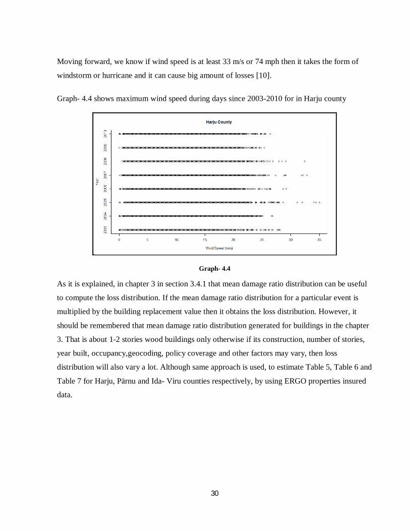
Graph- 4.4 shows maximum wind speed during days since 2003-2010 for in Harju county
Graph- 4.4
As it is explained, in chapter 3 in section 3.4.1 that mean damage ratio distribution can be useful
to compute the loss distribution. If the mean damage ratio distribution for a particular event is
multiplied by the building replacement value then it obtains the loss distribution. However, it
should be remembered that mean damage ratio distribution generated for buildings in the chapter
3. That is about 1-2 stories wood buildings only otherwise if its construction, number of stories,
year built, occupancy,geocoding, policy coverage and other factors may vary, then loss
distribution will also vary a lot. Although same approach is used, to estimate Table 5, Table 6 and
Table 7 for Harju, Pärnu and Ida- Viru counties respectively, by using ERGO properties insured
data.

31
Harju County
Categorize Windstorm
Windstorm Windstorm Mean damage ratio of building
Maximum loss of total Insured value to portfolio(EUR) Wind speed range(m/s) Wind speed (m/s)
1 14-18 16 0.003 13,900,479 2 18-22 20 0.03 139,004,793 3 22-26 24 0.09 417,014,378 4 26-30 28 0.26 1,204,708,204 5 30-34 32 0.39 1,807,062,306 6 34-38 36 0.49 2,270,411,615 7 38-42 40 0.66 3,058,105,440 8 42-46 44 0.85 3,938,469,127 9 46-50 48 0.96 4,448,153,368
10 50-54 52 1 4,633,493,091 Table 5
Table 5, expresses probable maximum loss correspondence to wind speed ranges. It other words,
for example if the wind speed range is 30-34 then its correspondence mean damage ratio to the
building is 0.39 and all the properties in the insured portfolio (to be assumed 1-2 stories wood
only). Otherwise loss and mean damage ratio to building may vary a lot as discussed previously.
Graph- 4.5 shows maximum wind speed during days since 2004-2010 for in Pärnu county.
Graph- 4.5

32
Parnu county
Categorize Windstorm
Windstorm Windstorm Mean damage ratio of building
Maximum loss of total Insured value to portfolio(EUR) Wind speed range(m/s)
Wind speed (m/s)
1 14-18 16 0.003 1,325,336 2 18-22 20 0.03 13,253,359 3 22-26 24 0.09 39,760,078 4 26-30 28 0.26 114,862,447 5 30-34 32 0.39 172,293,670 6 34-38 36 0.49 216,471,535 7 38-42 40 0.66 291,573,904 8 42-46 44 0.85 375,511,846 9 46-50 48 0.96 424,107,496
10 50-54 52 1 441,778,642 Table 6
Table 6 and Table 7, express probable maximum loss correspondence to wind speed ranges. It
other words, for example if the wind speed range is 34-38 then its correspondence mean damage
ratio to buildings is 0.49 and all the properties in the insured portfolio (to be assumed 1-2 stories
wood only). Otherwise loss and mean damage ratio to building may vary a lot as discussed
previously.
Graph- 4.6 shows maximum wind speed during days since 2003-2010 for in Ida-Viru county
Graph- 4.6

33
Ida- Viru County
Categorize Windstorm
Windstorm Windstorm Mean damage ratio of building
Maximum loss of total Insured value to portfolio(EUR) Wind speed range(m/s)
Wind speed (m/s)
1 14-18 16 0.003 1,775,774 2 18-22 20 0.03 17,757,738 3 22-26 24 0.09 53,273,215 4 26-30 28 0.26 153,900,399 5 30-34 32 0.39 230,850,598 6 34-38 36 0.49 290,043,060 7 38-42 40 0.66 390,670,244 8 42-46 44 0.85 503,135,920 9 46-50 48 0.96 568,247,627
10 50-54 52 1 591,924,612 Table 7
Graph- 4.7, 4.8, 4.9 show maximum wind speed during days since 2003-2010 for in Saare,
Lääne, Viljandi counties respectively.
Graph- 4.7

34
Graph- 4.8
Graph- 4.9

35
Graph- 4.10 shows maximum wind speed during days since 2003-2008 for in Lääne-Viru county.
Graph- 4.10
4.2 Flood loss distribution
If we discuss about Estonia then almost twenty areas in Estonia which are more vulnerable to
flood it includes Tallinn, Pärnu and Tartu counties. Municipalities like Häädemeeste, Hanila and
Haaslava. As coastal sea levels, snowmelt and rainfall are increasing due to climate change this is
making many of these areas at risk [8]. Specially, we should think about the most vulnerable
region for flood such as Pärnu and Lääne counties and South-West part of Estonia. The length of
Lääne and Pärnu county coastline are 400 km and 242 km respectively.
Flood loss distribution of Estonia, rest Baltic States and Scandinavia is presented in this part of
the thesis. Baltic States and Scandinavia loss distribution are important as there is lack of
historical data in Estonia. Hence, by creating such a scenario may help to show more appropriate
estimation in case of Estonia.
4.2.1 Flood loss distribution in Baltic States and Nordic countries during 1990 -2010
Flood loss distribution is estimated in the form of return period. For example, we can assume the
99th percentile, corresponding to the 100-year return period. The maximum loss occurred during

36
20-years time may underestimate the relevance of a given risk, but in many of the scenarios this
is the only feasible solution to get an estimate of the risk.
Graph 4.11-4.16, express the maximum historical total loss caused by flood in Estonia, Latvia,
Lithuania, Finland, Sweden during 1990-2010 as a percentage of its own according to 2010 GDP
respectively. These graphs also explains, exceedance probability of losses with respect to any
event. For example in graph 4.11 flood loss distribution is reaching 4% of Estonian GDP (2010)
at 99.8th percentile. It is corresponding to 500-year return period (1/500=0.2% => 100-0.2=
99.8%). So, chance of flood loss distribution to exceed 4% of Estonian GDP is 0.2% in any one
year.
Graph- 4.11
0.0%
1.0%
2.0%
3.0%
4.0%
5.0%
98.0% 98.5% 99.0% 99.5% 100.0%
% o
f 201
0 G
DP
Percentile
Flood loss distribution - Estonia
Total Losses

37
Graph- 4.12
Graph- 4.13
0.0%0.5%1.0%1.5%2.0%2.5%3.0%3.5%4.0%
98.0% 98.5% 99.0% 99.5% 100.0%
% o
f 201
0 G
DP
Percentile
Flood loss distribution - Latvia
Total Losses
0.0%
0.5%
1.0%
1.5%
2.0%
2.5%
3.0%
3.5%
98.0% 98.5% 99.0% 99.5% 100.0%
% o
f 201
0 G
DP
Percentile
Flood loss distribution - LithuaniaTotal Losses

38
Graph- 4.14
Graph- 4.15
Graph 4.16 describes the maximum historical total loss due to storm in European countries
during 1990-2010 as a percentage of its own according to 2010 GDP [7].
0.0%0.5%1.0%1.5%2.0%2.5%3.0%3.5%4.0%
98.0% 98.5% 99.0% 99.5% 100.0%
% o
f 201
0 G
DP
Percentile
Flood loss distribution - FinlandTotal Losses
0.0%
1.0%
2.0%
3.0%
4.0%
5.0%
98.0% 98.5% 99.0% 99.5% 100.0%
% o
f 201
0 G
DP
Percentile
Flood loss distribution - SwedenTotal Losses

39
Graph- 4.16
Due to lack of data graphs from 4.11-4.16 are created by using information and data provided in: Source: For historical total losses is the Emergency Events Database (EM-DAT) (Europe)
Source: Joint research centre- JRC- European Commission -Version September [7]
Think about Estonian flood distribution in graph 4.11, it shows that 1%, 0.5%, 0.2% probability
that loss exceed 1.55%, 1.8%, 4% respectively of Estonian GDP in a single year according to
2010 GDP but now if we see Estonian storm loss distribution in graph 4.16, it is 0.8% of
Estonian GDP in a single year. Why it is discussing over here reason is that if we are looking
individual loss distributions of flood or storm then it seems not so worst but if we add up both the
loss distribution due to flood and storm then loss distribution increases significantly and it can
create potential loss to Estonian insurance companies.
0.00%
0.50%
1.00%
1.50%
2.00%
2.50%
FI HU PL IT CY CZ IE LT PT AT ES DE GR BE NL UK SK LU FR SE SI EE DK LV
%of
201
0 G
DP
Country
Storm - maximum historical losses
Total Losses

40
Chapter 5
Conclusion
Estonia is considered to be less vulnerable to natural catastrophe. It is a sigh of relief for
insurance companies over here. However, it cannot be ignored that there is no Nat cat risk. There
have been seen several big and small storms; floods in recent years. According to climate change
scenario, coastal sea level is rising and poles ice melting. So there exists some risk which may
create big damage and loss.
In 2005, when the storm hit in Estonia, it created a big amount of loss. But insurance sector did
not impact a lot, the reason being, at that time there were not so many people had insured their
properties. Still there is no compulsory disaster insurance in Estonia, though we have to agree
that the risks related to natural catastrophe and man-made catastrophe are covered relatively
modestly by insurance contracts. People are being aware about catastrophe risk cover in
insurance and they prefer to take a policy which provides coverage of catastrophe risk. So in
future, if such a big event occurs then it may make significant losses to the insurance sector
without having a proper catastrophe modeling strategy.
Estonia is the least populated country and population density plays an key role in in deciding the
loss which occurs due to catastrophe events. Because of the scattered inhabitation of Estonia, the
local windstorms can be damaging, but not on a huge scale. As it is already discussed individual
risk is not exceeding to Nat cat retention, but if we combined two perils- windstorm and flood in
coastal areas which can cause severe damage to the property and this can count potential losses to
insurance companies. So it can be worked on this approach. This approach is so valuable for
insurance companies in Estonia because in this case loss can exceed their paying capacity. So,
insurance companies can be careful in future. In such a scenario insurance company can diversify
its risk to reinsurer by buying treaties or ceding its exceeding paying limit to coinsurer.
It is true that the data is not available of Nat cat events in Estonia as there are no so many
previous historic events. In this condition better to make possible approximation by creating

41
some scenarios. In other words, it is really interesting to use neighboring countries like
Scandinavia and Finland historical Nat cat events data. So it can assess the probability that
something similar may occur in future here.

42
Bibliography
[1] Haanpää, S., Lehtonen, S. , Peltonen, L., Talockaite, E. 2007, Impacts of winter storm Gudrun of 7th–9th January 2005 and measures taken in Baltic Sea Region, This was European Union funded research The Astra project
[2] Grossi , P. , Kunreuther, H. and Windeler 2005, An Introduction to Catastrophe Models and Insurance, Springer, pp 24-41
[3] Rockett, P. 2007, Catastrophe bond risk modelling, Published by Risk Management Solutions
[4] Latchman, S. , Quantifying the risk of natural catastrophes, published by AIR Worldwide
[5] Daneshvaran, S. and Haji, M. 2012, Long term versus warm phase, part II: hurricane loss analysis, Risk Finance, Vol. 13(2), pp 118-132
[6] Stubbs, N. and Perry, D. 1999, Documentation of a methodology to compute structural damage and content damage in a wind environment, Clemson University
[7] Maccaferri, S., Cariboni, F. and Campolongo, F. 2011, Natural Catastrophes: Risk relevance and Insurance Coverage in the EU, This is a report published by European Union [8] Suursaar, U., Sooäär, J. 2007, Decadal variations in mean and extreme sea level values along the Estonian coast of the Baltic Sea, TELLUS, Vol. 59(A), pp 249–260 [9] Andersan, R. and Dong, W. 1998, Pricing catastrophe reinsurance with reinstatement provisions using a catastrophe model, Forum Casualty Actuarial Society, pp 303-322 [10] Jaagus, J. and Kull, A. 2011, Changes in surface wind directions in Estonia during 1966-2008 and their relationships with large-scale atmospheric circulation, Estonian Journal of Earth Sciences, Vol. 60(4), pp 220-231 [11] Smith, T. 2010, Wind safety the building envelope, The National Institute of Building Sciences

43
Non-exclusive licence to reproduce thesis and make thesis public
I, KAPIL SHARMA________________________________________________________________
(author’s name)
(date of birth: ______10/12/1986___________________________________________),
1. herewith grant the University of Tartu a free permit (non-exclusive licence) to:
1.1. reproduce, for the purpose of preservation and making available to the public, including for addition to the DSpace digital archives until expiry of the term of validity of the copyright, and
1.2. make available to the public via the web environment of the University of Tartu, including via the DSpace digital archives until expiry of the term of validity of the copyright,
Natural catastrophe modeling for pricing in insurance
__________________________________________________________,
(title of thesis)
Supervised by Kalev Pärna __________________________________________________________,
(supervisor’s name)
2. I am aware of the fact that the author retains these rights.
3. I certify that granting the non-exclusive licence does not infringe the intellectual property rights or rights arising from the Personal Data Protection Act.
Tartu/Tallinn/Narva/Pärnu/Viljandi, 19.05.2014