NATO Reference MobilityModel (NRMM) Modeling of

, the DEMO III ExperimentalUnmanned, Ground Vehicle (XUV)

by Timothy T. Vong, Gary A. Haas, and Caledonia L. Henry

itFtL-m-435 April 1999

Approved for public release; distribution is unlimited.

-n

,

The findings in this report are not to be construed as an officialDepartment of the Amy position unless so designated by otherauthorized documents.

Citation of manufacturer’s or trade names does not constitute auofficial endorsement or approval of the use thereof.

Destroy this report when it is no longer needed. Do not returnit to the originator.

Army Research LaboratoryAberdeen Proving Ground, MD 2 1005-5066

ARL-MR-435 April 1999

.

.

NATO Reference Mobility Model(NRMM) Modeling of the DEMO IIIExperimental Unmanned GroundVehicle (XUV)

Timothy T. Vong, Gary A. Haas, and Caledonia IL. HenryWeapons and Materials Research Directorate, ARL

Approved for public release; distribution is unl&ited.

The Advanced Weapons Concepts Branch, Army Research Laboratory (ARL), was asked toassess and evaluate the predicted cross-country performance of the current DEMO IIIExperimental Unmanned Ground Vehicle (XUV) chassis design using the NATO ReferenceMobility Model (NRMM) by the Program Manager of the Department of Defense sponsoredDEMO III XUV Program. The XUV modeled approximately 2,500 lb that will be able totraverse cross-country terrain at 20 mph. The XUV is designed to be driven by an autonomousmobility package, but the NRMM does not support autonomous mobility; so, for the purposesof this study, the chassis was modeled as a manned vehicle. Currently, the XUV is in the finalchassis and suspension development phase by the systems integrator, Robotic SystemsTechnology, Inc. The NRMM is a computer-based simulation tool that can predict a vehicle’ssteady-state operating capability (effective maximum speed) over specified terrain. The NRMMcan perform on-road and cross-country prediction of a vehicle’s effective maximum speed. TheNRMM is a matured technology that was developed and proven by the Waterways ExperimentStation (WES) and the Tank-automotive and Armaments Command (TACOM) over severaldecades. The NRMM has been revised and updated throughout the years; the current versionused to perform this analysis is version 2, also known as NRMM II. ARL, was also asked tocompare the predicted performance of the XW chassis against the high-mobility, multipurpose,wheeled vehicle (HMMWV) using NRMM II. This report details the NRMM II analysis andassessment of the DEMO III XUV and WES HMMWV.

.

.

.

ii

Acknowledgments

The authors would like to thank those who provided valuable information and/or

help. They are:

l Richard B. Ahlvin, U.S. Army Waterways Experiment Station (WES)

l Bailey T. Haug, U.S. Army Research Laboratory (ARL)

l Jeffrey S. Robertson, Robotic Systems Technology, Inc. (RST)

l Bradley Beeson, Robotic Systems Technology, Inc. (RST)

. . .111

INTENTIONALLY LEFT BLANK

i v

.

Table of Contents

Acknowledgments ............................................................................ iii

List of Figures ................................................................................ vii

List of Tables .................................................................................. ix

1. Introduction . . . . . . . . . . . . . . . . . . . . . . . . . . . . . . . . . . . . . . . . . . . . . . . . . . . . . . . . . . . . . . . . . . . . . . . . . . . . . . . . . . . . 1

2. VEHDYN II Module ......................................................................... 3

2.1 Input Data .................................................................................... -42.2 Results ........................................................................................ 42.3 Discussions ................................................................................... 5

3. Obstacle-Crossing Module ................................................................ 6

3.1 Input Data.. .................................................................................. .63.2 Results ........................................................................................ 73.3 Discussion .................................................................................... 7

4. NRMM Main Module ........................................................................ 8

4.1 Input ........................................................................................... 94.2 Results ...................................................................................... .104.3 Discussion.. ................................................................................ .13

5. Conclusions. . . . . . . . . . . . . . . . . . . . . . . . . . . . . . . . . . . . . . . . . . . . . . . . . . . . . . . . . . . . . . . . . . . . . . . . . . . . . . . . . . .15

6. References . . . . . . . . . . . . . . . . . . . . . . . . . . . . . . . . . . . . . . . . . . . . . . . . . . . . . . . . . . . . . . . . . . . . . . . . . . . . . . . . . . . . . 17

Appendix A: NRMM Main Module. . ..I.............................................. 19

Appendix B: VEHDYN II Module.. . . . . . . . . . . . . . . . . . . . . . . . . . . . . . . . . . . . . . . . . . . . . . . . . . .45

Appendix C: Obstacle-Crossing Module . . . . . . . . . . . . . . . . . . . . . . . . . . . . . . . . . . . . . . . . . . . 49

Distribution List . . . . . . . . . . . . . . . . . . . . . . . . . . . . . . . . . . . . . . . . . . . . . . . . . . . . . . . . . . . . . . . . . . . . . . . . . . . . . 53

Report Documentation Page. . . . . . . . . . . . . . . . . . . . . . . . . . . . . . . . . . . . . . . . . . . . . . . . . . . . . . . . . . . ..55

V

.

INTENTIONALLY LEFT BLANK

vi

List of Figures

Figure a

1. Conceptual Rendering of DEMO III XUV ................................................... 1

2. VEHDYN II Module Schematic .............................................................. .3

3. XUV3 and WES HMMWV Dynamic Terrain Results ..................................... .4

4. XUV3 and WES HMMWV Dynamic Geometry Results .... . . . . . . . . . . . . . . . . . . . . . . . . . . . . . . . 5

5. Obstacle-Crossing Module Schematic .... . . . . . . . . . . . . . . . . . . . . . . . . . . . . . . . . . . . . . . . . . . . . . . . . . . . . .6

6. Diagram of Standard Trapezoidal Obstacle .... . . . . . . . . . . . . . . . . . . . . . . . . . . . . . . . . . . . . . . . . . . . . . . . 6

7. Obstacle-Crossing Failure Comparison of XUV3 and HMMWV ........................ .7

8. NRMM Main Module Schematic .... . . . . . . . . . . . . . . . . . . . . . . . . . . . . . . . . . . . . . . . . . . . . . . . . . . . . . . . . . . 9

9. Comparison of Velocity Profiles .............................................................. 10

10. Go Factors for HMMWV and XUV3 ...... . . . . . . . . . . . . . . . . . . . . . . . . . . . . . . . . . . . . . . . . . . . . . . . . 12

11. No-Go Factors for XUV3 and HMMWV................................................. .13

12. Scatter Plot by Terrain Element.. .. . . . . . . . . . . . . . . . . . . . . . . . . . . . . . . . . . . . . . . . . . . . . . . . . . . . . . . . . . .14

13. Scatter Plot by Terrain Element, by XUV3 Limiting Factor .... . . . . . . . . . . . . . . . . . . . . . . . . . 14

A-l. Comparison of Velocity Profiles for Dry/Fall Europe ..... . . . . . . . . . . . . . . . . . . . . . . . . . . . . . . 40

A-2. Comparison of Velocity Profiles for Dry/Fall SW Asia.. .............................. .40

A-3. Comparison of Velocity Profiles for Wet/Fall Europe ................................. .41

A-4. Comparison of Velocity Profiles for Wet/Fall SW Asia ............................... .41

A-5. Scatter Plot by Terrain Element for Dry/Fall Europe ..... . . . . . . . . . . . . . . . . . . . . . . . . . . . . . . .42

A-6. Scatter Plot by Terrain Element for Dry/Fall SW Asia .... . . . . . . . . . . . . . . . . . . . . . . . . . . . . . . 42

A-7. Scatter Plot by Terrain Element for Wet/Fall Europe ..... . . . . . . . . . . . . . . . . . . . . . . . . . . . . . . .43

A-8. Scatter Plot by Terrain Element for Wet/Fall SW Asia .... . . . . . . . . . . . . . . . . . . . . . . . . . . . . . .43

B-l. Tire Deflection vs Load Curve ..... . . . . . . . . . . . . . . . . . . . . . . . . . . . . . . . . . . . . . . . . . . . . . . . . . . . . . . . .47

B-2. XUV3 Zero-Force Configuration. .... . . . . . . . . . . . . . . . . . . . . . . . . . . . . . . . . . . . . . . . . . . . . . . . . . . . . .48

vii

INTENTIONALLY LEFT BLANK

.

. . .Vlll

I -

List of Tables

Page

1. Average Difference for XUV3 and HMMWV Speed Profile.... . . . . . . . . . . . . . . . . . . . . . . . . . . 11

2. V-80 Speeds for HMMWV and XUV3 ...... . . . . . . . . . . . . . . . . . . . . . . . . . . . . . . . . . . . . . . . . . . . . . . . . 11

3. Difference of V-80 Speeds Between HMMWV and XUV3.. ............................ .l 1

4. Difference of Terrain Traversable Between HMMJVV and XUV3 ...................... .12

ix

INTENTIONALLY LEFT BLANK

.

x

1. Introduction

This report details the NATO Reference Mobility Model (NRMM) analysis and

performance assessment of the DEMO III Experimental Unmanned Ground Vehicle (XUV)

and a high-mobility, multipurpose, wheeled vehicle (HMMWV), and the comparison of their

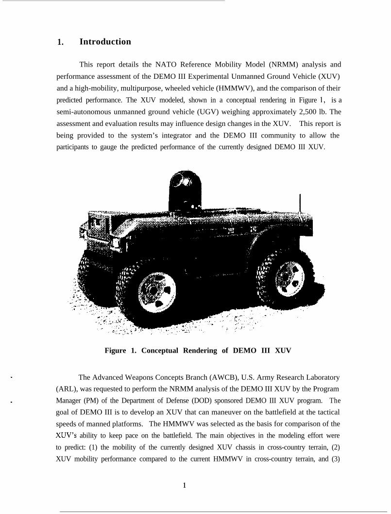
predicted performance. The XUV modeled, shown in a conceptual rendering in Figure 1, is a

semi-autonomous unmanned ground vehicle (UGV) weighing approximately 2,500 lb. The

assessment and evaluation results may influence design changes in the XUV. This report is

being provided to the system’s integrator and the DEMO III community to allow the

participants to gauge the predicted performance of the currently designed DEMO III XUV.

--_

Figure 1. Conceptual Rendering of DEMO III XUV

The Advanced Weapons Concepts Branch (AWCB), U.S. Army Research Laboratory

(ARL), was requested to perform the NRMM analysis of the DEMO III XUV by the Program

Manager (PM) of the Department of Defense (DOD) sponsored DEMO III XUV program. The

goal of DEMO III is to develop an XUV that can maneuver on the battlefield at the tactical

speeds of manned platforms. The HMMWV was selected as the basis for comparison of the

XUV’s ability to keep pace on the battlefield. The main objectives in the modeling effort were

to predict: (1) the mobility of the currently designed XUV chassis in cross-country terrain, (2)

XUV mobility performance compared to the current HMMWV in cross-country terrain, and (3)

1

the ability of the XUV chassis to meet the required DEMO III exit criteria to traverse cross-

country terrain at 20 mph. This criteria has been interpreted by the DEMO III community to

mean that a HMMWV can traverse at 25 to 30 mph. The system’s integrator, Robotic Systems

Technology, Inc. (RST), is currently in the final chassis and suspension development phase

for the XUV. AWCB was asked to assess and evaluate the cross-country performance of the

current DEMO III XUV design using NRMM. The HMMWV modeled was the M 1025,

armament carrier version. The U.S. Army Waterways Experiment Station (WES), the

developer of the NRMM, provided the model of the HMMWV.

The NRMM is a computer-based simulation tool that is widely accepted in the mobility

community as a means to predict a vehicle’s steady-state operating capability (effective

maximum speed) over specified terrain. The NRMM can perform predictions of a vehicle’s

effective maximum speed on-road and cross-country. The NRMM is a mature technology that

was developed and proven by the WES and the U.S. Army Tank-automotive and Armaments

Command (TACOS) over several decades. The NRMM has been revised and updated

throughout the years; the current version that was used to perform this analysis is version 2,

also known as NRMM II.

The NRMM is divided into three separate primary modules: (1) a vehicle dynamics

module (VEHDYN II), (2) an obstacle-crossing performance module (OBS78B), and (3) a

primary prediction module (NRMM Main). These three program codes are run independently.

The VEHDYN II and obstacle-crossing programs process generic obstacle and terrain data sets

that produce vehicle specific results that become inputs for the main predicting module’s

vehicle data. During processing, the main module accesses these data to obtain a prediction

appropriate for the specific terrain being processed [ 11. This report details the work involved

within each module and the results relative to the DEMO III XUV. The WES HMMWV results

used for the comparison in the VEHDYN II and obstacle-crossing modules were obtained from

WES. The WES HMMWV NRMM Main input file is listed in Appendix A.

The mobility predictions presented in this paper are intended to facilitate comparison

between the vehicle designs, not to predict actual vehicle performance. NRMM predictions

explicitly assume the frailties of a human driver and implicitly assume the capabilities of a

human driver. While the XUV is designed as an unmanned vehicle, there has been no attempt

to compensate the NRMM mobility performance predictions for this difference. Therefore, the

predictions for the XUV may differ substantially from what is achieved by the actual vehicle

for reasons associated with its unmanned nature, not from its chassis design.

2

2. VEHDYN II Module

.

.

The VEHDYN was originally developed in 1974 in support of the Army Mobility

Model (AMM). In 1978, the AMM and its supporting VEHDYN were adopted as the standard

references for evaluating the cross-country mobility performance of vehicles by a NATO

working group. The AMM was subsequently renamed the NRMM. The adoption of NRMM

and VEHDYN as NATO standards brought about widespread use and modifications.

Unfortunately, this caused numerous inconsistencies, programming errors, redundant

variables, and an unwieldy program. In 1986, to remedy this situation, the VEHDYN was

rewritten to include many of the changes and renamed VEHDYN II [2].

The VEHDYN II is a two-dimensional (2-D) vehicle dynamics model. As shown in

Figure 2, the user provides a vehicle description set, terrain and geometry set, and threshold

limits. The vehicle description is specific to the studied vehicle. The terrain, geometry, and

threshold limits used are VEHDYN II standards that are provided and known. The terrain

(surface roughness) units are measured in root mean-square (RMS) values varying from O-6

ins RMS. The geometries are half-rounds measuring from O-l 8 inch. Once all the proper

input parameters are given, the program is executed and the output is obtained using 6 W and

2.5 g’s (gravity) as threshold values. These threshold values are steady-state tolerance levels

of human drivers derived from years of experimental testing by WES and TACOM to validate

the NRMM.

Input

VehicleDescription

Terrain &Geometry

ThresholdLimits

Program

w Vehic leDynamics

Output

w, Maximum Speedat Threshold Limits

Figure 2. VEHDYN II Module Schematic

The final output from VEHDYN II is two resultant graphs. One graph is the maximum

speed vs. surface roughness (inches RMS), the other is maximum speed vs. half-rounds

(inches). Further explanation of VEHDYN II can be obtained from the users manual [ 21.

3

2.1 Input Data

The XUV is refered to as XUV3 in this report to match the configuration control of the

DEMO III effort. The majority of the XUV3 vehicle input data is obtained from RST

suspension design data, revision 3, dated 7/98. The vehicle specifications obtained from RST

are the spring data, shock data, various vehicle dimensions, and weight characteristics. The

tire data were derived from ARL and Aberdeen Testing Center (ATC) testing. Test data were

obtained for numerous operating pressures of the tire. All other parameters in the input data

file were derived from hand calculations using various formulas, most using the previously

mentioned parameters as input. The actual VEHDYN II input files are found in Appendix B.

The VEHDYN II users manual gives a more detailed description of the data files and its input

parameters, if the reader is interested.

2.2 Results

Figures 3 and 4 are the compiled dynamic results of VEHDYN IT for the XUV3 vs. the

WES HMMWV. The results are evaluated at the thresholds of 6 W for the terrain and 2.5 g’s

for the half-round bumps.

Maximum Speed vs. Surface Roughnessat 6 Watts Threshold

0 OS I 1.5 2 2.5 3 3.5 4 4.5 5 5.5 6

Surface Roughness (inches RMS)

Figure 3. XUV3 and WES HMMWV Dynamic Terrain Results

4

Maximum Speed vs. Half-Roundsat 2.5 Gs Threshold

.

.

Figure 4. XUV3 and WES HMMWV Dynamic Geometry Results

2.3 Discussions

60

50

10

0 2 4 6 8 IO 12 14 16 18 20

Half-Round (inch)

.

From the vehicle dynamics aspects and using the stated threshold values, the DEMO III

XUV performs similar to the HMMWV. For most of the terrains and bumps, they are only

separated by a few miles per hour. They are separated by larger margins for values of terrain

and bump height, where each vehicle is limited by its maximum speed ability. The XUV3,

with its current drivetrain configuration, has a calculated maximum speed of 40 mph, The

HMMWV is limited to 60 mph. Although the true HMMWV maximum speed might be greater

than 60 mph, for the purposes of our analysis, it was capped at 60 mph since maximum

HMMWV speed was not our focus. From the curves, if the maximum speed is either 40 or 60

mph, it means their maximum speeds are not limited by the 6 W or 2.5 g’s threshold but by

factors not modeled. In order for the XUV3 to meet the DEMO III performance goals, it has to

be able to traverse cross-country terrain at 20 mph. One suggested interpretation of this

criterion is that the XUV3 traverse terrain at 20 mph that a manned HMMWV traverses at 25 to

30 mph. From Figure 3, this corresponds to terrain with a surface roughness of approximately

1.0 in RMS. On terrain of this sort, the VEBIDYN II model predicts that the XUV3 is ride-

quality limited at 23 mph.

3. Obstacle-Crossing Module

The obstacle-crossing module is a 2-D program that calculates a vehicle’s ability to

cross an obstacle set. Its output to NRMM Main, summarized in Figure 5, is the minimum

clearance (or maximun interference) and the maximun propulsive force needed to override the

obstacles in the set specific to each vehicle.

InputProgram

VehicleDescription

ObstacleGeometry

ObstacleCrossing

Output

f+iq

Figure 5. Obstacle-Crossing Module Schematic

These obstacle geometries are standard trapezoidal shapes, shown in Figure 6. The

obstacle set for a wheeled vehicle is made up of combinations of three height levels, three

width lengths and eight approach angles (122” to 248 ‘).

W i d t h

IHeight

I

Figure 6. Diagram of Standard Trapezoidal Obstacle

Since the angles are greater and less than 180” (flat if 1 SO”), the obstacle set includes

both positive and negative obstacles. More detail can be obtained from the users

3.1 Input Data

manual [3].

The majority of the XUV3 vehicle input data for obstacle crossing

gravity, ground clearance profile, and vehicle front/rear weight distribution were

the RST suspension design data, revision 3, dated 7/98. Other parameters

like center of

obtained from

not explicitly

obtained fi-om RST were derived from hand calculations of various formulas, using the RST

6

parameters as input. The actual obstacle crossing input files are found in Appendix C. The

obstacle crossing users manual [3] gives a more detailed description of the data files and input

parameters, if the reader is interested.

3.2 Results

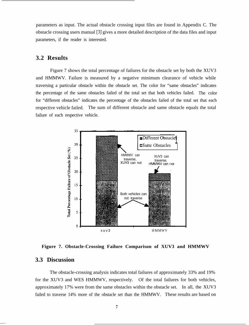
Figure 7 shows the total percentage of failures for the obstacle set by both the XUV3

and HMMWV. Failure is measured by a negative minimum clearance of vehicle while

traversing a particular obstacle within the obstacle set. The color for “same obstacles” indicates

the percentage of the same obstacles failed of the total set that both vehicles failed. The color

for “different obstacles” indicates the percentage of the obstacles failed of the total set that each

respective vehicle failed. The sum of different obstacle and same obstacle equals the total

failure of each respective vehicle.

aDifferent Obstacle

&Same Obstacles

HMMWV can XUV3 cantraverse,

XUV3 can nottraverse,

Uh&lW\I P2l-l I

Both vehicles cannot traverse

:S1

x u v 3 HMMWV

Figure 7. Obstacle-Crossing Failure Comparison of XUV3 and HMMWV

3.3 Discussion

The obstacle-crossing analysis indicates total failures of approximately 33% and 19%

for the XUV3 and WES HMMWV, respectively. Of the total failures for both vehicles,

approximately 17% were from the same obstacles within the obstacle set. In all, the XUV3

failed to traverse 14% more of the obstacle set than the HMMWV. These results are based on

7

all the obstacles in the set. Since a subset of these obstacles is used in each theater scenario

selected for the NRMM Main, the obstacle-crossing difference in the final analysis can vary

from these results. The obstacle-crossing failures can be attributed to any of several vehicle

characteristics like clearance height, wheel base, or front and rear overhangs affecting the

angles of approach and departure.

4. NRMM Main Module

The primary output of the NRMM Main Module is the prediction of speed-made good

of a given vehicle over specified terrain. Speed-made good is the effective maximum speed in

the long run, and takes into account not only pure physical factors, such as powertrain

capability, terrain grade, and traction available from soil of a specific type, but also subjective

factors, such as driver tendency to slow down over uneven surfaces or in low visibility, A

complete description is given in Ahlvin and Haley [ 11. The NRMM is typically run over a

collection of terrain units representative of an area of terrain, and the speed-made-good is

represented as a profile of terrain area traversable at speed, ordered from highest speed to

lowest. Another profile is the “accumulated” speed profile, which represents the average

speed-made-good over the least difficult terrain.

Another perspective of interest is the particular factor limiting the speed of the vehicle

over the terrain element. For off-road terrain, it is of particular interest which factor caused the

vehicle to be unable to traverse a terrain unit, a condition known as “No-Go”. The NRMM

calculates (accumulates) the proportion of the terrain where speed-made-good is limited by each

of 13 factors, and the proportion of the terrain made untraversable by each of 9 factors. A

block diagram description is shown in Figure 8.

In this study, the mobility of the XUV3 is compared to that of the HMMWV in two

theaters under two weather conditions. Results are tabulated in a form that facilitates

comparison of speed and accumulated-speed profiles, Go/No-Go statistics, and Go/No-Go

factor statistics. This study was limited to comparison of pure vehicular mobility as predicted

by the NRMM, which implicitly assumes the capabilities and explicitly allows for the

vulnerabilities of a human driver. The study did not attempt to address differences in mobility

resulting from the robotics nature of the XUV.

8

VehicleSpeed-

made-good

Terrain NRMM

No-Go

Figure 8. NRMM Main Module Schematic

4.1 Input

Vehicle data have a number of components, including vehicle geometry, mass

distribution characteristics, tire characteristics, tractive force curve (the force that can be applied

to the ground by the drivetrain, as a function of ground speed), threshold curves from the

obstacle-crossing and ride-quality modules, braking performance information, and miscellany

such as the height of the driver’s eyes above the ground. The bulk of this information was

provided by RST or derived by ARL from RST data. The source of individual data items is

documented in line-by-line comments in Appendix A, section A.1. For the HMMWV, a

vehicle description in NRMM format was provided by WES.

The terrain is described as a collection of homogeneous terrain elements statistically

representative of the overall terrain. Each terrain element is described in terms of grade, soil

type, seasonal surface strength, vegetation characteristics (stem size and density), seasonal

visibility distance, surface roughness, and obstacle size and geometry (trenches and mounds).

Terrain used for the comparison was NRMM terrain files representative of Europe and

Southwest Asia. Data for these theaters is part of the NRMM package distributed by the

NRMM program office.

Scenario data contains generic data that are independent of vehicle and terrain, such as

weather conditions, vegetation override strategy, etc. For this study, the scenario was

modified to evaluate both dry and wet/slippery conditions in each theater. (The wet/slippery

condition represents standing water from a recent rain during an average wet season.) To

9

avoid an unmanageable number of variables, all scenarios were run in October foliage

conditions.

4.2 Results

Velocity profiles of the two vehicles over both theaters, and both wetness conditions

were similar in that the XUV3 was several miles per hour slower over the entire terrain than

was the HMMWV, and the HMMWV could traverse somewhat more terrain than could the

XUV. A representative velocity profile is shown in Figure 9. Other profiles are in Appendix

A, section A.6.

XUV-3 vs HMMWV Cumulative Terrain at SpeedDry Fall Europe

0 10 20 3 0 40 50 60 70 60 9 0 100

Terraln (%)

+HMMWV speed +XUV-3 speed - HMMWV accumulated speed -XUV-3 accum speed

Figure 9. Comparison of Velocity Profiles

10

The average difference, in mph, between the two profiles is tabulated in Table 1.

Table 1. Average Difference for XUV3 and HMMWV Speed Profile

Average Europe SW Asia

difference

Dry 1.7 3.6

Wet 1.9 2.9

A more commonly used comparison is between the so-called “V-80” speed of the two

vehicles, taken from the accumulated speed profiles. The V-80 speed is the average speed of

the vehicle over the easiest (highest achieved speed) 80% of the terrain. V-80 speeds are

tabulated in Table 2, and their differences tabulated in Table 3. Note that V-70 speeds (average

speed over the easiest 70% of the terrain) were used for the Wet Europe condition, as V-80

speeds were not defined.

Table 2. V-80 Speeds for HMMWV and XUV3

Vehicle

HMMWVDRY

x u v 3

HMMWVWET

x u v 3

* Indicates V-70 Speed

Europe

17.3

15.9

17.2”

15.3”

SW Asia

15.6

14.8

15.6

14.2

Table 3. Difference of V-80 Speeds Between HMMWV and XUV3

Delta MPH 1 Europe 1 SW Asia

* Indicates V-70 Speed

11

Also of interest are differences in the amount of terrain that can be traversed, and the

reasons limiting the speed. The difference in the amount of terrain traversable is tabulated in

Table 4. In Figures 10 and 11, the NRMM program printouts of these values have been

reformatted to emphasize the contrast. Figure 10 presents the percent of terrain that can be

traversed by each vehicle, along with a table of speed limiting factors. Figure 11 presents the

percent of terrain that could not be traversed. The results from Southwest Asia under

wet/slippery conditions were not graphed because they were nearly identical to those from the

dry conditions.

Table 4. Difference of Terrain Traversable Between HMMWV and XUV3

Delta % Europe

Dry 4.4

Wet 4.0

SW Asia

1.2

1.2

1 0 0

9 0

6 0

7 0

1 6o

fj 50

54 0

83 0

2 0

1 0

0

92.56 88.04 94.11 92.93 86.92 82.93

t _-____--~--.---i

.- ..-.- _-. .-_

o~aneu~r~ud xe~ bmobti j-. 0.36 0 . 2 1 o,33 _ . . .._-0.29~ __In Qbstacle impact 1 . 0 7 0 . 5 3 0.18 1.02 0.4I0 Soil & v e g e t a t i o n r e s i s t a n c e 3 . 2 2 4 . 5 9 0 . 2 1 5.63 4.38

n Tire Soeed Limit 1 2 . 1 6 1 4 . 0 6 6 . 1 8_ _ _ _ _ _ _ _•I Maneuver around obs and veg 1 1 . 0 6 2 . 6 2 9 . 2 7 1.75 9.61 2.61

~0 Obstacle override force 2 7 . 2 4 ; 1 9 . 9 9 . 7 5 7.5 25.41 16.49 ~EI VisibWtv 2 1 . 1 4 3 7 . 6 3 ! 1 1 . 4 2 16.36 1 23.56 39.43 1a Ride Qualitv 1 6 . 2 9 2 2 . 3 6 ; 4 9 . 4 65.14 : 12.96 17.33 I

Figure 10. Go Factors for HMMWV and XUV3

12

t-----_’ -I_

16.92I

16 --_-_- ..-. __--.-----..~

14 __~._-~..~~--_---~-_~__-- .-___- - - - - - ..---- - -

g 12

ti

3 lo

g *

6

4

2

0

.

n Obstacle Override

p soil

I n Tipping

:~Kj Belly in!erference..

n Vegetation Override

q Brakicg

CI Soil resistance

q Obstacle interference

H M M W V xuv3 H M M W V xuv3 H M M W V x u v 3

0 . 3 7

0.79

1.17

5.03

0.43

0.81

1.15

9.33

0.62

5.24 7.03

0.52 0.59

2.24 2.28

5.54 5.28

4.67 8.77

Figure 11. No-Go Factors for XUV3 and HMMWV

4.3 Discussion

An interesting comparison is a scatter plot comparing each vehicle’s speed over the

same terrain element, shown in Figure 12. The overall shape (generally following the line with

slope 1.0) reinforces the notion that the XUV3 is slightly slower but generally comparable to

the HMMWV over the same terrain. Questions are raised by the spike at HMMWV speed of

12 mph, and by the deterministic-looking set of points tracking a line with slope roughly 0.8.

A variant of this plot (shown in Figure 13), with point color keyed to the limiting factor, is

enlightening. From this graph and others like it, oddities in the shape of the plot can be

explained. The mysterious vertical spike comes from a 12-mph speed limit imposed by the tire

inflation pressure selected by the HMMWV model for traversing sandy soil. The tire pressure

prescribed for the XUV3 is suitable for speeds up to the vehicle top speed, so there is no

corresponding horizontal spike. The line at slope 0.8 is composed of terrain units where

visibility is the limiting factor. NRMM models visibility as a linear function of the height of the

driver’s eye (for XUV3, the height at the top of the bodywork was taken as the likely location

of the driving sensors), so it makes sense that the comparison is also linear.

13

XUV-3 vs HMMWV by Terrain Element .Dry Fall Europe

3 0

1 0

5 1t

0 I

5 1 0 1 5 2 0 2 5 3 0 3 5 4 0

H M M W V s p e e d ( m p h )

Figure 12. Scatter Plot by Terrain Element

XUV-3 vs HMMWV by Terrainand XUV-3 Factor

Dry Fall Europe

,, _. . ^.. _ . . ” __.

l

_--

Unit .

i

-i

i

_A1 0 1 5 2 0 2 5

H M M W V s p e e d ( m p h )

3 0 3 5 4 0

,.vegetalion o v e r r i d e

, obstacle clearance

+obslacle impact

xsoil, slope, & veg r e s i s t a n c e

# m a n e u v e r a r o u n d obsl & veg

-obstacle overr ide force

yvisibilily

ride dynamics

Figure 13. Scatter Plot by Terrain Element, by XUV3 Limiting Factor

14

Many of the terrain elements that are traversed faster by the XUV3 are speed-limited by

the necessity of maneuvering around objects. It is reasonable that the narrower, shorter XUV3

with its tighter turning circle can maintain a higher speed in these circumstances.

The Go/No-Go predictions also deserve a closer analysis. Note that in each case the

No-Go statistics for both vehicles are dominated by obstacle interference and the XUV3 is able

to traverse several percent less terrain than is the HMMWV. In fact, the difference in obstacle

interference completely accounts for the difference in No-Go statistics. Obstacle crossing in

NRMM is a table lookup process from data output by the model described in section 3, and is

thus a completely 2-D process. The larger tires and higher centerline ground clearance of the

HMMWV are the probable explanation for the HMMWV’s advantage in this domain.

The Go factors are more complicated to analyze. There are big differences in the

factors governing the speed at which the two vehicles can traverse terrain, though the overall

differences in speed attained remain fairly small, as shown in Tables 1 and 3. It is surprising

to note that the much more powerful HMMWV is limited by the “obstacle override force” factor

substantially more often than is the XUV3, but a closer look at the “by terrain element” data

reveals that the XUV3 is limited by the “ride-quality” and “visibility” factors over that same

terrain, at speeds very much the same. Further study is necessary to make sense of all the Go

factor data.

5. Conclusions

The predicted mobility of the XUV3 was qualitatively similar to that of the HMMWV in

both the European and Southwest Asian theaters and under conditions of dry and wet/slippery

soil. In general, the model predicted the XUV3 could traverse a few percent less of the terrain

than the HMMWV, at speeds averaging 2-4 mph slower than the HMMWV. The limiting

factors resulting in the increased No-Go statistics were consistent with the lower tractive force

and lower ground clearance of the XUV3. Limiting factors resulting in the decrease in ground

speed were consistent with lower tractive force and lower sensor height of the XUV3. So the

results were consistent with expectation and with trade-offs made in the design of the XUV3.

The 2-4 mph decrease in predicted average speed over terrain in comparison to the

HMMWV satisfies the “20 mph over terrain a HMMWV can traverse at 25 to 30 mph” criterion

proposed by some as a test of adequacy for the small chassis. The results are primarily based

on differences in vehicle chassis characteristics. Other than eye height, the same driver

constraints are used for the HMMWV and the XUV3. This evaluation of the performance of

15

the XUV3 has pointed to the need for further research in the effects of autonomous mobility on

UGV mobility evaluations. The effects of autonomous mobility technology on vehicle speed

over terrain are yet to be assessed. Future efforts at ARL will model these effects, but proof

will have to await testing of the XUV3 in suitably challenging terrain.

16

6. References

1. Ahlvin, D., and P. Haley. “NATO Reference Mobility Model Edition II, NRMM IIUser’s Guide.” Technical Report Number GL-9% 19, U.S. Army WaterwaysExperiment Station, Corps of Engineers, Vicksburg, MS, December 1992.

2. Creighton, D. “Revised Vehicle Dynamics Module: User’s Guide for ComputerProgram VEHDYN II.” Technical Report Number SL-86-9, U.S. ArmyWaterways Experiment Station, Corps of Engineers, Vicksburg, MS, May 1986.

3. Haley, P., M. Jurkat, and P. Brady, Jr. “NATO Reference Mobility Model, Edition IUsers Guide, Volume II.” Technical Report Number 12503, U.S. ArmyTank-automotive and Armanments Command, Warren, MI, October 1979.

17

INTENTIONALLY LEFT BLANK

18

.

.

Appendix A:NATO Reference Mobility Model (NRMM) Main Module

19

A.1 Vehic1.e Data Input File for Experimental Unmannned Ground

Vehicle 3 (XUV3): XUV3.dat

XUV3, DEMO III UGV (RST Inc)Project: XUV Ver 3Date entered: 20 August 1998!Date revised: 20 August 1998; Timothy VongFile name:XUV3.STDDescription:

XUV3, DEMO III UGV (RST Inc), ver# corresponds t oJeff Robertson ver#$VEI-IICLE!**Basic information

NAMBLY= 2,WGHT( l)= 1182,13 18, ! Jeff Robertson chassis info dated 7/27/98

! **Geometric informationCGH =27.0, ! Jeff Robertson chassis info dated 7/27/98CGLAT = 0.0,CGR = 35.0, ! Jeff Robertson 7/27/98 (horizontal, cg to rear axle)CL = 12.0, ! Jeff Robertson chassis info dated 7/27/98

! (Ground clearance = @ ctr of hull, min. elsewhere,CLRMIN( 1)=9.5,9.5, !Tim calculation from Jeff 7/27/98 (@wheel arm!)!VAA = 90, !TR-GL-92- 17!VDA = 45, !TR-GL-92- 17

! **Recognition distance informationEYEHGT=42.0, ! FWP report (top of vehicle)

! **Vegetation performance informationNVUNTS = 1,PBF =1600, !Max push bar force(lb), assumedPBHT = 12.0, ! assumed(bumper)VULEN( l)=l 11 .O, ! Jeff Robertson 7/27/98 (74+18.5+18.5) (vehicle length)WDTH =65.8, ! Jeff Robertson 7/27/98 (56+98)(vehicle width)

! **Aerodynamic informationACD = .8, ! Brad Beeson calculation sheetPFA = 13.5, ! Tim calculated (ft”2)

! **Traction assembly informationNVEH(1) = l,l,TL=74.0, ! Jeff Robertson 7/27/98 (wheel base)

! WI(l) = !n/u, NRMM II; NRMM-mgrWT( 1) =56.0,56.0, ! Jeff Robertson 7/27/98 (front/rear width tire center)WTE(l) =46.2,46.2, ! tire Sect. width (9.8”) (front/rear width tire inside)

! **Track informationASHOE =, !N/AGROUSH(I) =, !N/ANBOGIE(l) =, !N/ANFL(l) =, !N/ANPAD(1) =, !N/ARW(1) =, !N/ATRAKLN(1) =, !N/ATRAKWD(l) =, !N/A

! **Wheel/tire informationAVGC=63, ! [lbs/deg] (cornering/lateral stiffness/her. spring rate)

! assume 10% of wheel load if none of previous available, Nancy Saxon; 10% of (591+659)/2AXLSP( 1) =74.0, ! Jeff Robertson 7/27/98 (axle spacing)

2 0

NJPSI = 1,DF’LCT(1,1)=0.663,0.705, ! ARL Measured (25 psi Avg. load 591 front, 659 rear)!DFLCT(l,1)=1.2,1.7, !HWY!DFLCT( 1,3)=1.6,2.2, !SAND!DFLCT( 1,4)=1.8,2.4, !EMERDIAW( 1) =29.0,29.0, !Dunlop Tire Inc.ICONST( 1)= 1,1, ! 1 =Radial2=BiasID(l) = O,O,IT(l) = 0,0,JVPSI = 1,KCTIOP(l)= 1,1,1,1,1,1,1,1,

KTSFLG(l)= l,l, !O=stiffness ignored l=flexible 2=medium 3=stiffNCHAIN( I)= 0,0,NWHL(1) = 2,2,RDIAM( 1) = 15.0,15.0, !front,rear from DUNLOP Tire Inc.RIMW(1) = 6.5,6.5, !front,rear from DUNLOP Tire Inc.SECTH( 1) = 7.0,7.0, !front,rear from DUNLOP Tire Inc.SECTW(1) =9.8,9.8, ! DUNLOP Tire Inc.TIREID( l)=‘Dunlop Radial Mud Rover LT235/75Rl S’,‘Same as front ‘,TPLY( 1) =6,6,TPSI(1,1)=25,25, ! ARL data!TPSI( 1,2)=23,23, !cold inflation pressure for single tire loads at!TPSI(1,3)=17,17, !speeds of 5,12,40 and 60 mph PSI’S chosen were!TPSI(1,4)=15,15, !for tire load of 25001bs although Ml025 tireVTIRMX( l)=lOO,lOO !mph, assumed at 25 psi, conversation with Jeff

!**Side-slope performance information; “zeroed” to remove slippage for NRMM calculationHROSUS( 1) = ! 15.0, 15.0; (Roll Center) Conversation with Jeff Robertson, RSTNSUSP = ! 2; derived from VEHDYNIIRAID( 1) = ! 146.0, 165.0; derived 7/27/98 presentation, RST(f=lO23/7, r=l157/7)

‘**Powertrain: fax received from AM general information FEB.94i fax no. 62252561-xls 2/2/94 BGV & 6225256H.XLS 2/l/94 BGV! IAPG =, ! n/u, NRMM-II

IP(1) =l,l,!**Powertrain: engine information (from Kubota brochure, provided by!Anthony DeMarco of Engine Distributors, Inc. (800)220-2700! CID= 61.12, !Kubota D1005-B( E model are same)! IDIESL= 1,! IENGIN= 3, !number of data pts. describing r-pm vs torque curve! TARDEC origin unknown! ENGINE(2,1)= 1600,34, !net continuous rpm vs torque! ENGINE(2,2)= 2400,34, !net continuous r-pm vs torque! ENGINE(2,3)= 3600,33, !net continuous rpm vs torque! HPNET =22.5, !net continuous hp! NCYL = 3,! N E N G = 1 ,! QMAX =34, !maximum net continuous torque! **Power-train: transmission information! ICONVl=O,! C O N V l = , ,! ICONV2= 0,! CONV2= , ,! ITCASE = 0, ! not used in NRMM-II! ITRAN = 1, ! not used in NRMM-II! ITVAR = 1,! KTROPR= 8*0, !Best=O! LOCKUP = 0,

21

! NGR = 0,! NTRANG = 1,! TCASE(l)=l.O,l.O,! TQIND = ,! TRANS(l,l,l)=l,l,! * *Powertrain: Final drive information

FD(l) =l,l,LOCDIF= 1,REVM( 1) =695.5,695.5, !USED DFLCT OF 0” TO CALCULATE (Mile* 12/2*pi*r)

! **Power-train: Braking informationIB(l) =l,l,XBRCOF= 8, ! assume same as used by M 1025 HMMWV run

! **Powertrain: n-active force vs. speed! TF FROM Brad Beeson calculations at 60 Hp curve

IPOWER=lO! SPEED(mph) TF(lbs) HP

POWER= 0.000000 1600.00 ! 0.0000001 .ooooo 1600.00 ! xx6.5000 1600.00 ! xx12.0000 1200.00 ! xx15.0000 825.00 ! xx20.0000 675.00 ! xx25.0000 575.00 ! xx30.0000 475.00 ! xx35.0000 400.00 ! xx38.0000 350.00 ! xx

! **Ride dynamics dataMAXL= 1 ,ABSPWR( l)= 6,MAXIPR=12, !VEHDYNII Run + Excel Sheet Compiled (xuv3.vd2,8/98)KVRIND( l)= 1,

RMS(1)=0,.19,.34,.66,.86,1.20,1.81,2.17,3.27,3.49,4.0,5.0! Speed (mph) at 6-WATTS

VRIDE(1,1,1)=40,40,40,24.57,24.57,19.69,9.56,8.6,7.29,6.7,6.21,5.0! **Obstacle height-speed

NHVALS =9, ! VEHDYNII Run + Excel Sheet Compiled (xuv3.vd2,8/98)KOHIND( 1) = 1,HVALS(l) =0,1,2,3,4,6,8,10,18,

! Speed (mph) at 2.5gs over obstacle heightVOOB(l,l) =40,40,40,40,40,17.93,10.05,3.37,2.38,

! **Ride: Obstacle spacing vs. speed! NSVALS =! SVALS =! VOOBS =! * *Water crossing information

CD = .7,DRAFT=,FORDD =30,SAE =58,SAI =69,VFS = 5,vss = ,VSSAXP= ,WC =,WDAXP= ,

! **NRMM-mgr

2 2

NWR =,WDPTH( l)= ,WRAT(l) = ,WRFORD= ,

ENDNOHGT !OBS78B Version of: 24 April, 1990

-3 !Date: 20-August-1998NANG !Vehicle file: XUV3.VEH

8 !Obstacle file: WHEELS.OBSNWDTH

3CLRMININCHES

8.85-3.75

-21.108.85-3.70

-10.778.85-3.05-3.438.852.542.488.263.542.978.751.06-2.079.96

-1.30-4.4511.507.81-3.228.85-3.81

-18.758.85-2.12-2.848.851.981.788.855.515.518.404.464.538.340.870.058.06

FOOMAX FOO HOVALS AVALS WVALSPOUNDS POUNDS INCHES RADIANS INCHES963.0 38.4 3.15 1.95 5.88

2000.1 95.8 15.75 1.95 5.882001.6 185.2 33.46 1.95 5.88971.4 34.9 3.15 2.48 5.88

1005.1 126.7 15.75 2.48 5.88795.0 124.4 33.46 2.48 5.88660.4 42.2 3.15 2.69 5.88648.5 108.6 15.75 2.69 5.88

1031.6 122.5 33.46 2.69 5.88390.1 33.3 3.15 2.86 5.88356.2 55.5 15.75 2.86 5.88689.1 96.5 33.46 2.86 5.88397.6 39.8 3.15 3.42 5.88429.0 75.1 15.75 3.42 5.88689.1 102.5 33.46 3.42 5.88673.4 47.2 3.15 3.60 5.88728.0 134.1 15.75 3.60 5.88911.3 133.7 33.46 3.60 5.88590.2 14.0 3.15 3.80 5.88

1114.2 126.8 15.75 3.80 5.881241.1 208.0 33.46 3.80 5.88276.4 1.8 3.15 4.33 5.88861.3 25.0 15.75 4.33 5.88

2199.2 149.1 33.46 4.33 5.881009.4 25.4 3.15 1.95 29.882043.1 123.8 15.75 1.95 29.881903.4 123.7 33.46 1.95 29.88971.4 28.1 3.15 2.48 29.88963.2 79.3 15.75 2.48 29.88

1266.6 154.3 33.46 2.48 29.88661.0 31.4 3.15 2.69 29.88504.2 50.5 15.75 2.69 29.88973.5 130.4 33.46 2.69 29.88390.1 28.7 3.15 2.86 29.88428.6 59.2 15.75 2.86 29.88689.1 102.1 33.46 2.86 29.88397.6 34.9 3.15 3.42 29.88428.5 61.5 15.75 3.42 29.88689.1 105.6 33.46 3.42 29.88674.8 33.7 3.15 3.60 29.88734.0 107.9 15.75 3.60 29.88

1036.8 142.8 33.46 3.60 29.88961.1 35.1 3.15 3.80 29.88

2 3

-1.50 1123.1 131.1 15.75 3.80 29.88-4.65 1255.6 164.6 33.46 3.80 29.888.06 1039.8 41.4 3.15 4.33 29.88

-7.65 2217.0 171.8 15.75 4.33 29.88-99.00 2217.0 171.8 33.46 4.33 29.88

8.85 977.9 13.2 3.15 1.95 141.60-3.75 2205.0 72.1 15.75 1.95 141.60

-10.44 2324.3 154.0 33.46 1.95 141.608.85 1038.2 17.2 3.15 2.48 141.601.31 1133.6 75.0 15.75 2.48 141.60-0.16 1266.6 146.3 33.46 2.48 141.608.85 673.5 16.6 3.15 2.69 141.603.68 728.7 63.5 15.75 2.69 141.603.61 973.5 125.2 33.46 2.69 141.608.85 397.7 16.0 3.15 2.86 141.606.70 428.6 61.5 15.75 2.86 141.606.71 689.1 94.2 33.46 2.86 141.608.99 397.5 18.2 3.15 3.42 141.606.74 427.9 61.2 15.75 3.42 141.606.64 689.1 93.2 33.46 3.42 141.608.85 674.6 19.4 3.15 3.60 141.603.74 729.1 68.8 15.75 3.60 141.603.57 1031.5 128.2 33.46 3.60 141.609.05 1038.2 17.3 3.15 3.80 141.601.28 1121.5 76.0 15.75 3.80 141.60-0.14 1265.0 162.1 33.46 3.80 141.608.85 1061.3 21.1 3.15 4.33 141.60

-3.50 2205.2 71.8 15.75 4.33 141.60-10.15 2297.7 156.3 33.46 4.33 141.60

A.2 Vehicle Data Input File for U.S. Army Waterways Experiment

Station (WES) High-Mobility, Multipurpose, Wheeled Vehicle

(HMMWV): M1025wes.dat

HMMWV, M1025, ARMAMENT CARRIER (WES STANDARD)Project: Standard VehicleDate entered: 10 MARCH 94File name:M1025.STDDescription:HMMWV, M1025, ARMAMENT CARRIER (WES STANDARD)$VEHICLE

! **Basic informationNAMBLY= 2,WGHT( 1)=3000,4500, !TM 9-2320-280-10

! **Geometric informationCGH =32.8, !AMC GENERAL FAX FEB 94CGLAT = 0,CGR =50.5, !AMC GENERAL TR-GL-92-7C L =11.3, !TR-GL-93- 15

! (Ground clearance = @ ctr of hull, min. elsewhere,CLRMIN(l)=11.3,11.3, !TR-GL-93-15

24

!VAA = 90, !TR-GL-92- 17!VDA = 45, !TR-GL-92- 17

! **Recognition distance informationEYEHGT=62, !GL-93-15

! **Vegetation performance informationNVUNTS = 1,PBF =7500, !TM9-2320-280-10PBHT =24.8, !GL-93- 15VULEN( 1 )= 180, !TM9-2320-280- 10WDTH =85, !TM9-2320-280- 10

1 **Aerodynamic information.ACD = .7,PFA =35.3, !AMC General Fax Feb94

! **Traction assembly informationNVEH(l) = l,l,TL=130, ! TR-GL-92- 17

! WI(l) = !n/u, NRMM II; NRMM-mgrWT(1) =71.6,71.6, !TR-GL-93-15WTE(l) =59.1,59-l, !TR-GL-93-15

! **Track informationASHOE =, !N/AGROUSH( 1) =, !N/ANBOGIE(l) =, !N/ANFL(l) =, !N/ANPAD(1) =, !N/ARW(1) =, !N/ATRAKLN(l) =, !N/ATRAKWD(l) =, !N/A

! **Wheel/tire informationAVGC=l88,AXLSP(1) =130,NJPSI = 4,DFLCT( 1 ,1)=1.2,1.7, !HWY See note on PSI input for Source of PSI’s andDFLCT( 1,2)=1.4,1.9, !CC Deflections calculated from Goodyear load, PSIDFLCT( 1,3)=1.6,2.2, !SAND Deflection curve MD-327477 2/7/92DFLCT(1,4)=1.8,2.4, !EMERDIAW( 1) =36.6,36.6,!GOODYEARICONST(l)= l,l,ID(l) = 0,0,IT(l) = 0,0,JVPSI = 1,KCTIOP( l)= 1,1,3,2,3,3,2,3,KTSFLG( l)= 1 ,1, ! 1 =Radial2=BiasNCHAIN( l)= O,O,NWHL(l) = 2,2,RDIAM(1) =16.5,16.5, !TireidRIMW(1) = 8.25,8.25, !MD-409522SECTH(1) = 9.2,9.2, !Wes Field Tests, lo-1990SECTW( 1) =12.3,12.3, !Goodyear MD-409522TIREID( l)=’ 37X1 2.5R16.5LT RADIAL1,‘37X12.5R1 6.5LT RADIAL ‘,TPLY (1) =4,4,TPSI( 1,1)=26,26, !Fax from Joe Ripley Goodyear 4/5/93 table minimumTPSI( 1,2)=23,23, !cold inflation pressure for single tire loads atTPSI(1,3)=17,17, !speeds of 5,12,40 and 60 mph PSI’S chosen wereTPSI(1,4)=15,15, !for tire load of 25OOlbs although Ml 025 tireVTIRMX( 1)=60,40,12,5, !load were 1500 for front and 2250 for rear & R.Jones

25

!**Side-slope performance informationHROSUS( 1) =, ! to be derived from VEHDYN dataNSUSP =, ! to be derived from VEHDYN dataRAID( 1) =, ! assumes roll center is C-G;

l**Powertrain: fax received from AM general information FEB.94I fax no. 62252561-xls 2/2/94 BGV & 6225256H.XLS 2/l/94 BGV! IAPG =, ! n/u, NRMM-II

IP(1) =l,l,! **Powertrain: engine information

CID= 379,IDIESL= 1,IENGIN= 0,

! TARDEC origin unknownENGINE=HPNET =15d, (TM-9-2320-280- 10NCYL = 8, !TM-9-2320-280-10NENG = 1,QMAX =239,

‘**Powertrain: transmission information’ ICONVl=O,CONVl= , ,ICONV2= 0,CONV2= , ,

! ITCASE = 0, ! not used in NRMM-II!ITRAN =l, ! not used in NRMM-IIITVAR = 0,KTROPR = 8*0, !Best=OLOCKUP = 1,NGR = 6,NTRANG = 1,TCASE(l)=l.O,l.O,TQIND = ,TRANS( 1,1,1)=6.47,.96,

3.86,.96,2.61,.96,2.48,.96,1.48,.96,1.0 ,.96,

!**Powertrain: Final drive informationFD( 1) =4.92,.96,LOCDIF= 1,REVM( 1) =583,583, !USED CC DFLCT OF 2.0” TO CALCULATE

! **Powertrain: Braking informationIB(l) =l,l,XBRCOF= .8,

‘**Powertrain: tractive force vs. speedi TEMPLE’S FILES-NO DOCUMENTED SOURCE! IPOWER= 2 1,! POWER= 0,7550,! 1 ,6840,! 2 ,6185,! 3 ,5690,! 5 ,4760,! 7,4195,! 9,4100,! 11 ,3785,

26

! 13 ,249.5,I 19,2265,! 22,1721,I; 27 ,1600,

29 ,1550,t 31 955,)Ii 35 40 ,950, ,930,! 45 ,890,! 50,655,! 60,640,! 70 ,600,I 73 ,600,i TF FROM AMC GENERAL SCAAN DATA 2-l-94

IPOWER=! SPEED TF HP

POWER= 0.000000 5880.00 ! 0.0000001 .ooooo 5880.002.00000 5880.003 .ooooo 5880.004.00000 5880.005.00000 5638.006.00000 5122.037.00000 4744.078.00000 4690.769.00000 4602.2010.0000 4444.9711 .oooo 4269.8612.0000 2867.7613 .oooo 2860.8214.0000 2841.2315.0000 2805.0216.0000 2753.9717.0000 2689.9718.0000 2628.2919.0000 2555.7820.0000 2490.252 1 .oooo 1952.4222.0000 1935.7723.0000 1914.3724.0000 1887.4025 .OOOO 1857.4626.0000 1829.3127.0000 1800.0228.0000 1764.9129.0000 1731.1330.0000 1592.053 1 .oooo 1565.9532.0000 1092.4933.0000 1091.4334.0000 1089.6435 .oooo 1087.3836.0000 1084.4537.0000 1081.0038.0000 1076.0039.0000 1070.23

! 15.6800! 31.3600! 47.0400! 62.7200! 75.1733! 81.9524! 88.5559! 100.069! 110.453! 118.533! 125.249! 91.7683! 99.1751! 106.072! 112.201! 117.503! 121.945

26.15829.49332.81309.33613.56517.41520.79423.83 1

! 126.832! 129.602! 131.780! 133.874! 127.364! 129.452! 93.2258! 96.0454! 98.7944! 101.489! 104.108! 106.659! 109.035! 111.304

27

!FROM PETER HALEY’S VEHICLE FILE HMMWV-WC-HIGH!IPOWER = 141

SPEED TF~POWER= 0.000000

HP2893.00 ! 0.000000

0.500000 2834.25 ! 3.77900!!!!!!!!!!!!

1 .ooooo 2775.50 ! 7.401331.50000 2716.75 ! 10.86702.00000 2658.00 ! 14.17602.50000 26 14.25 ! 17.42833.00000 2570.50 ! 20.56403.50000 2526.75 ! 23.58304.00000 2483.00 ! 26.48534.50000 2441.25 ! 29.29505 .ooooo 2399.50 ! 31.99335.50000 2357.75 ! 34.58036.00000 23 16.00 ! 37.0560

40.000041 .oooo42.000043.000044.000045 .oooo46.000047.000048.000049.000050.00005 1 .oooo52.000053.000054.000055.000056.000057.000058.000059.000060.00006 1 .OOOO62.000063.000064.000065 .OOOO66.000067.000068.000069.000070.00007 1 .oooo72.000073.000074.000075 .oooo76.000077.000078.000079.0000

1063.921056.281048.021038.991029.481019.941011.121002.23993.245982.456971.171960.41195 1.206943.08 1743.197741.438

I

113.485115.487117.379119.137120.793122.393124.030125.613127.135128.374129.489130.616131.901133.289107.020108.744

739.354 ! 1 0.410737.27 1 ! 1 2.065734.430 ! 1 3.59273 1.477 ! 1 1 5.086728.117 ! 1 6.499724.35 1 ! 1 1 7.828720.55 1 ! 1 1 9.131716.469 ! 120.367712.388 ! 121.581708.084 ! 122.735703.667 ! 123.845699.333 ! 124.948695.412 ! 126.101691.490 ! 127.234687.272 ! 128.291682.872 ! 129.290678.390 ! 130.251673.305 ! 131.070668.220 ! 131.862663.168 ! 132.634658.126 ! 133.380653.581 ! 134.202649.846 ! 135.168646.112 ! 136.114

28

!!!!!!!!!!!!!!!!!!!!!!!!!!!!!!!!!1

i

I!!!!!!!I

i

!!!!!!!1

!!!

6.50000 2279.257.00000 2242.507.50000 2205.758.00000 2169.008.50000 2134.259.00000 2099.509.50000 2064.7510.0000 2030.0010.5000 1996.0011 .oooo 1962.0011.5000 1928.0012.0000 1894.0012.5000 1859.7513.0000 1825.5013.5000 1791.2514.0000 1757.0014.5000 1721.7515.0000 1686.5015.5000 1651.2516.0000 1616.0016.5000 1604.0017.0000 1592.0017.5000 1580.0018.0000 1568.0018.5000 1566.7519.0000 1565.5019.5000 1564.2520.0000 1563.0020.5000 1559.752 1 .oooo 1556.502 1.5000 1553.2522.0000 1550.0022.5000 1544.5023 .OOOO 1539.0023.5000 1533.5024.0000 1528.0024.5000 1516.2525.0000 1504.5025.5000 1492.7526.0000 1481.0026.5000 1480.7527.0000 1480.5027.5000 1480.2528.0000 1480.0028.5000 1348.7529.0000 1217.5029.5000 1086.2530.0000 955.00030.5000 954.5003 1 .oooo 954.0003 1.5000 953.50032.0000 953.00032.5000 952.75033.0000 952.50033.5000 952.25034.0000 952.000

! 39.5070! 41.8600! 44.1150! 46.2720! 48.3763! 50.3880! 52.3070! 54.1333

55.888057.552059.125360.608061.991763.284064.4850

! 65.5947! 66.5743! 67.4600! 68.2517! 68.9493! 70.5760! 72.1707! 73.7333! 75.2640! 77.2930! 79.3187! 81.3410! 83.3600! 85.2663! 87.1640! 89.0530! 90.9333! 92.6700

; g-g;;! 97:7920! 99.0617! 100.300! 101.507! 102.683! 104.640! 106.596! 108.552! 110.507! 102.505! 94.1533! 85.4517! 76.4000! 77.6327! 78.8640! 80.0940! 81.3227! 82.5717! 83.8200! 85.0677! 86.3147

29

! 34.5000?i

35.000035.5000

! 36.0000! 36.5000! 37.0000! 37.5000! 38.00001 38.5000! 39.0000! 39.5000! 40.0000! 40.5000! 41.0000! 41.5000! 42.0000! 42.5000! 43.0000! 43.5000! 44.0000! 44.5000! 45.0000! 45.5000! 46.0000! 46.5000! 47.0000! 47.50001

i48.000048.5000

! 49.0000! 49.5000! 50.0000! 50.5000! 51.0000! 51.5000! 52.0000! 52.5000! 53.0000! 53.5000! 54.0000! 54.5000! 55.0000! 55.5000! 56.0000! 56.5000! 57.0000! 57.5000! 58.00001

I58.500059.0000

! 59.5000! 60.0000! 60.5000! 61.0000I

I61.500062.0000

950.167948.333946.500944.667942.833941.000939.167937.333935.500933.667931.833930.000925.667921.333917.000912.667908.333904.000899.667895.333891.000886.667882.333878.000850.375822.750795.125767.500739.875712.250684.625657.000656.400655.800655.200654.600654.000653.400652.800652.200651.600651.000649.900648.800647.700646.600645.500644.400643.300642.200641.100640.000638.000636.000634.000632.000

! 87.4153! 88.5111! 89.6020! 90.6880! 91.7691'i 93.9167 92.8453

! 94.9831! 96.0447! 97.1013! 98.1531! 99.2000! 99.9720! 100.732! 101.481! 102.219! 102.944! 103.659! 104.361! 105.052! 105.732! 106.400! 107.056! 107.701! 105.446! 103.118! 100.716! 98.2400! 95.6905! 93.0673! 90.3705! 87.6000! 88.3952! 89.1888! 89.9808! 90.7712! 91.5600! 92.3472! 93.1328! 93.9168! 94.6992! 95.4800! 96.1852! 96.8875! 97.5868! 98.2832! 98.9767! 99.6672! 100.355! 101.039! 101.721! 102.400! 102.931! 103.456! 103.976! 104.491

30

! 62.5000 630.000 ! 105.000! 63.0000 628.000 ! 105.504! 63.5000 626.000 ! 106.003Ii

64.0000 624.000 ! 106.49664.5000 622.000 ! 106.984

! 65 .OOOO 620.000 ! 107.467! 65.5000 618.000 ! 107.944! 66.0000 616.000 ! 108.416! 66.5000 6 14.000 ! 108.883! 67.0000 6 12.000 ! 109.344! 67.5000 610.000 ! 109.800! 68.0000 608.000 ! 110.251Ii

68.5000 606.000 ! 110.69669.0000 604.000 ! 111.136

! 69.5000 602.000 ! 111.571! 70.0000 600.000 ! 112.000

! **Ride dynamics dataMAXL= 1,ABSPWR( l)= 6,MAXIPR=24, !TECHNICAL REPORT GL-92-7 Field Data or VEHDYNKVRIND( l)= 1,

RMS(1)=0,.45,.45,.47,.5,.55,.6,.65,.7,.8,.85,.9,.95,1,1.1,1.18,1.2,1.3,1.34, 1.47, 2, 2.2, 2.4, 6,

! 6 - W A T T S VRIDE(1,1,1)=l00,80,50,45,42,38,36,34,33,30,29,28,27,26.2,24,23,22.5,21,20,18,12,11,10.5,2,

! **Obstacle height-speedNHVALS =17, !TECHNICAL REPORT GL-92-7KOHIND( 1) =l ,HVALS(l) =0, 4, 4, 4, 4.2, 4.4,4.5,4.9,5,5.5,6.2,7,8,8.3,9.3,10,100,VOOB(l,l) =100,100,50,38,30,25.5,21,17,16,14.5,13,14,12,9,7,5,2,

! **Ride: Obstacle spacing vs. speed! NSVALS =! SVALS =! VOOBS =! **Water crossing information

CD = .7,DRAFT=,FORDD =30,SAE =58,SAI =69,VFS = 5,vss = ,VSSAXP= ,WC =,WDAXP= ,

! **NRMM-mgrNWR =,WDPTH(l)= ,WRAT(1) = ,WRFORD= ,

SENDNOHGT OBS78B Version of: 24 April, 1990

3 Date: 25-FEB-94 Time: 15:08:20NANG Vehicle file:M1025.OBV

8 Obstacle file:C:\MSD\OBMOD\OBW.DAT

31

NWDTH STEPMN= 1.0000 STEPMX= 2.00003

CLRMININCHES14.241.64

-16.0714.241.48

-16.0914.231.49

-11.4114.231.65

-0.2814.468.307.51

15.006.222.35

16.296.57

-2.6116.8315.178.71

14.241.64

-16.0714.241.48

-16.2014.231.47-5.9314.233.112.94

14.518.227.92

14.535.872.34

14.254.45-3.628.463.65

-18.0913.903.43

-9.6613.90

FOOMAX FOO HOVALS AVALS WVALSPOUNDS POUNDS INCHES RADIANS INCHES2996.4 105.4 3.15 1.95 5.886767.9 352.9 15.75 1.95 5.886774.2 562.6 33.46 1.95 5.882996.4 106.7 3.15 2.48 5.883429.8 329.4 15.75 2.48 5.883420.7 554.4 33.46 2.48 5.882249.6 82.4 3.15 2.69 5.882252.1 315.3 15.75 2.69 5.882169.5 411.3 33.46 2.69 5.881346.0 94.7 3.15 2.86 5.881346.1 257.0 15.75 2.86 5.881373.0 215.8 33.46 2.86 5.881357.7 89.7 3.15 3.42 5.881406.2 271.0 15.75 3.42 5.881477.2 252.9 33.46 3.42 5.882270.7 65.9 3.15 3.60 5.882363.0 297.1 15.75 3.60 5.882499.5 498.9 33.46 3.60 5.881553.5 35.5 3.15 3.80 5.883581.5 319.7 15.75 3.80 5.883807.2 580.4 33.46 3.80 5.88591.1 -2.5 3.15 4.33 5.88

2385.5 84.4 15.75 4.33 5.885835.3 209.7 33.46 4.33 5.882996.4 91.8 3.15 1.95 29.886767.9 312.3 15.75 1.95 29.886774.2 505.9 33.46 1.95 29.882996.4 92.8 3.15 2.48 29.883429.8 293.5 15.75 2.48 29.883420.7 504.7 33.46 2.48 29.882249.6 71.6 3.15 2.69 29.882252.1 283.5 15.75 2.69 29.882077.2 302.0 33.46 2.69 29.881346.0 82.8 3.15 2.86 29.881329.6 212.6 15.75 2.86 29.881477.5 231.8 33.46 2.86 29.881358.0 80.4 3.15 3.42 29.881406.2 235.7 15.75 3.42 29.881475.5 239.9 33.46 3.42 29.882278.8 79.4 3.15 3.60 29.882372.7 301.7 15.75 3.60 29.882507.3 399.1 33.46 3.60 29.882932.1 80.6 3.15 3.80 29.883619.8 334.0 15.75 3.80 29.883830.4 549.9 33.46 3.80 29.885609.7 184.4 3.15 4.33 29.887093.2 314.9 15.75 4.33 29.887410.2 575.5 33.46 4.33 29.882967.7 54.3 3.15 1.95 141.607118.4 209.5 15.75 1.95 141.607425.2 408.1 33.46 1.95 141.602967.7 54.7 3.15 2.48 141.60

32

4.26 3610.5 199.6 15.75 2.48 141.60-3.46 3834.6 396.5 33.46 2.48 141.6013.90 2277.8 57.5 3.15 2.69 141.605.54 2372.4 206.5 15.75 2.69 141.602.35 2502.5 350.1 33.46 2.69 141.60

13.97 1357.8 51.1 3.15 2.86 141.608.07 1406.1 175.5 15.75 2.86 141.607.93 1477.5 291.8 33.46 2.86 141.60

14.00 1358.0 48.7 3.15 3.42 141.608.11 1404.8 172.5 15.75 3.42 141.607.93 1477.0 290.6 33.46 3.42 141.60

13.98 2277.9 56.3 3.15 3.60 141.605.55 2368.7 201.7 15.75 3.60 141.602.34 2504.9 359.5 33.46 3.60 141.60

13.91 2802.3 41.1 3.15 3.80 141.604.42 3619.3 210.0 15.75 3.80 141.60-3.44 3835.8 401.0 33.46 3.80 141.6014.46 2908.5 40.0 3.15 4.33 141.603.61 7106.8 152.3 15.75 4.33 141.60

-17.21 7417.1 350.8 33.46 4.33 141.60

A.3 Example of Command Input File for XUV3: run.inp

! Anything after an ‘I! ” is ignored ! ! !ECHO=ON ! Enable echo of these input options on system output! input=kbd ! system input!output=con !run.out ! system output!scratch=SCRATCH ! Specify specific name for internal scratch files.pred=predhvflau ! prediction outputstats=stathvflau ! Statistics output! SPCL=special ! Enable special (traverse, acdc etc.) outputCALL =data\vehlist.inp ! Example of “call” to another input filesfile=data\scenario.dat ! scenario file! scenario=DRY-NORMAL ! scenario #1! scenario=WBT-NORMAL ! scenario #2! scenario=SNOW ! scenario #3! scenario=SAND ! scenario #4! scenario=WWET-SLIPRY ! scenario #5! scenario=WET-SLIPRY ! scenario #6scenario=WET-SLIPRO ! scenario #7!tvfile=terrain/cktem.a90 ! Terrain file (check patch)! tvfile=terrain/cktem.r90 ! Terrain filetvfile=tenain/5322.a90 ! Terrain file (LAUTERBACH)!tvfile=terrain/3254iv.a90 ! terrain file (MAFRAQ)! tvfile=terrain/2756IV.A90 ! terrain file (Honduras)!#VEH=2,1,3 ! (run 2 vehicles i.e. vehicle #l & #3)! (The following namelist may appear anywhere in the input or not at all.)$CONTRL

! DETAIL=1 0, ! When enabled, this will print all diagnostics! ! (Which is not recommended except for one terrain unit)! KVEH=l, ! When enabled, ethos vehicle data input! KMAP=l, ! When enabled, ethos terrain data input

33

!!!!!!!I

i1

!

KSCEN=l, ! When enabled, ethos scenario data inputThe above could also be accomplished by requestion the entire COMMOMname via the ‘vnames’ option as:VNAMES=‘VEHICL TERRAN SCEN’KTPP=l , ! When enabled, ethos inputs & outputs of terrain preprocessorKIV3 = 2 ! Would enable ‘low level’ diagnostics for routine IV3KIV(3)=2 ! Alternative to aboveKII( 11)=3* 1 ! Would enable diagnostics for routines II 11, II 12, & II 13KTFPLT= 1, ! When enabled, produces soil corrected TF vs. Speed plot for

! slope case KUDL = 1 (up-slope.)SEARCH=2, NTUX=1,5, ! Would run only 2 terrain units; #l & #5

VNAMES( 1 )=‘vcicmb’ ! When enabled, this will print combination VCI!$END

A.4 Example of Vehicle List File for XUV3: vehlist.inp

! 21 August 1998!List of vehicles for example!(This file is “Called” by main module system input)!VEHICLE= DATA’XUVl .DAT!VEHICLE= DATA\MlAl_F94.DAT!vehicle= DATA\M1025_M94.DAT! VEHICLE= datakndarse.dat!vehicle= data’mdars2.dat!vehicle= datab1025std.datVEHICLE= DATA’XUV3.DAT

A.5 Example of Scenario File for XUV3: scenario.dat

DRY-NORMALDry,Normal,October$SCENARMAPG=2,LAC=l,ISEASN=l, ISNOW= 0, ISAND= 0, ISURF= 1,NOPP=O, NSLIP= 0, MONTH= 10,

COEFHD= 1 .O,GAMMA=. 10,ZSNOW=lO.O,RDFOG=lOOO., REACT=.75, DCLMAX=2.0, SFTYPC=90.0,VBRAKE= 2.0, VISMNV= 2.0, VLIM= 100.0, VWALK= 4.0,

$ENDDRY,NORM,JUNDry,Normal,June$SCENAR!MAPG=2,LAC=l,ISEASN=l , ISNOW= 0, ISAND= 0, ISURF= I,NSLIP= 0, MONTH=6,

COEFHD= 1 .O,GAMMA=. 10,

3 4

ZSNOW=lO.O,RDFOG=lOOO., REACT=.75, DCLMAX=2.0, SFTYPC=90.0,VBRAKE= 2.0, VISMNV= 2.0, VLIM= 100.0, VWALK= 4.0,

$ENDWET-NORMALWet,Normal,October$SCENAR!MAPG=2,LAC=l,ISEASN=3, ISNOW= 0, ISAND= 0, ISURF= 1,NOPP= 0, NSLIP= 0, MONTH=lO,

COEFHD=l .O, GAMMA=. 10, ZSNOW=lO.O,RDFOG=lOOO., REACT=.75, DCLMAX=2.0, SFTYPC=90.0,VBRAKE= 2.0, VISMNV= 2.0, VLIM= 100.0, VWALK= 4.0,$END

WET,NORM,JANWet,Normal,January$SCENAR!MAPG=2,LAC=l,ISEASN=3, ISNOW= 0, ISAND= 0, ISURF= 1,NOPP= 0, NSLIP= 0, MONTH= 1,

’COEFHD=l .O, GAMMA=. 10, ZSNOW=lO.O,RDFOG=lOOO., REACT=.75, DCLMAX=2.0, SFI’YPC=90.0,VBRAKE= 2.0, VISMNV= 2.0, VLIM= 100.0, VWALK= 4.0,$END

WET-SLIPRYWet,Slippery,June$SCENAR!MAPG=2,LAC=l,ISEASN=3,ISNOW= 0,ISAND= 0,ISURF= 2,NOPP= 0,NSLIP= 1,MONTH=6,

COEFHD=l .O,GAMMA=. 10,ZSNOW=lO.O,

RDFOG=lOOO.,REACT=.75,DCLMAX=2.0,SFrYPC=90.0,VBRAKE= 2.0,VISMNV= 2.0,VLIM= 100.0,VWALK= 4.0,$END

WWET-SLIPRYWet-wet,Slippery,June$SCENAR!MAPG=2,LAC=l,ISEASN=4,

3 5

ISNOW= 0,ISAND= 0,ISURF= 2,NOPP= 1,NSLIP= 1,MONTH= 6,

COEFHD= 1 .O,GAMMA=. 10,ZSNOW= 10.0,

RDFOG= 1 OOO.,REACT=.75,DCLMAX=2.0,sFrYPc=90.0,VBRAKE= 2.0,VISMNV= 2.0,VLIM= 100.0,VWALK= 4.0,$END

SNOW~;yG~;~fW,January! MAPG=2,LAC=l ,ISEASN= 1,ISMODL= 1,ISNOW= 1,ISAND= 0,ISURF= 3,NOPP= 1,NSLIP= 0,MONTH= 1,COEFHD= 1 .O,GAMMA=. 10,ZSNOW=lO.O,

RDFOG=lOOO.,REACT=.75,DCLMAX=2.0,SFrYPC=90.0,VBRAKE= 2.0,VISMNV= 2.0,VLIM= 100.0,VWALK= 4.0,$ENDSNOW/ICE~so;Ec~ISURF=ICE,Soil=Dry,Visib=Januaxy

!MAPG=2,LAC= 1,ISEASN=l, !(DRY)MONTH= 1, !(January)ISAND= 0,NOPP= 1,NSLIP= 0,ISURF= 3, !(iCE)

ISMODL=l, ISNOW= 1, COEFHD=l .O, GAMMA=. IO, ZSNOW=lO.O,RDFOG=lOOO., REACT=.75, DCLMAX=2.0,

36

SFrYPC=90.0,VBRAKE= 2.0, VISMNV= 2.0, VLIM= 100.0, VWALK= 4.0,$END ’SNOW/DRYSgo;~w(~tSURF=DRY,Soil=Dry,Visib=January

!MAPG=2,LAC=l,ISEASN= 1, ! (DRY)MONTH= 1, !(January)ISAND= 0,NOPP= 1,NSLIP= 0,ISURF= 1, !(DRY)

ISMODL=l, ISNOW= 1, COEFHD=l .O, GAMMA=.1 0, ZSNOW=lO.O,RDFOG=lOOO., REACT=.75, DCLMAX=2.0,SRYPC=90.0,VBRAKE= 2.0, VISMNV= 2.0, VLIM= 100.0, VWALK= 4.0,$END

CRRELSNOWDry,Snow,January (new CRREL model)$SCENAR!MAPG=2,LAC=l,ISEASN= 1,ISNOW= 1,ISMODL=2,ISAND= 0,ISURF= 3,NOPP= 1,NSLIP= 0,MONTH= 1,

COEFHD=l .O,GAMMA=. 10,ZSNOW=lO.O,

RDFOG= 1 OOO.,REACT=.75,DCLMAX=2.0,SFrYPC=90.0,VBRAKE= 2.0,VISMNV= 2.0,VLIM= 100.0,VWALK= 4.0,$EN-DCRREL’ICESnow(CRREL),SURF=ICE,SOIL=DRY,VISB=January$SCENAR!MAPG=2,LAC=l,ISEASN=l , ! (DRY)ISNOW= 1, !(Yes)ISMODL=2, !(CRREL)ISAND- 0,ISURF= 3, !(ICE)NOPP= 1,NSLIP= 0,

37

MONTH= 1, ! (January)COEFHD= 1 .O,GAMMA=. 10,ZSNOW=lO.O,

RDFOG= 1 OOO.,REACT=.75,DCLMAX=2.0,SFrYPC=90.0,VBRAKE= 2.0,VISMNV= 2.0,VLIM= 100.0,VWALK= 4.0,$END

CRREL./DRYSnow(CRREL),SURF=DRY,SOIL=DRY,VISB=January$SCENAR! MAPG=2,LAC=l,ISEASN=l, !(DRY)ISNOW= 1, !(Yes)ISMODL=2, !(CRREL)ISAND= 0,ISURF= 1, ! (DRY)NOPP= 1,NSLIP= 0,MONTH= 1, !(January)

COEFHD= 1 .O,GAMMA=. 10,ZSNOW=lO.O,

RDFOG=lOOO.,REACT=.75,DCLMAX=2.0,SFrYPC=90.0,VBRAKE= 2.0,VISMNV= 2.0,VLIM= 100.0,VWALK= 4.0,$END

SANDDry,Sand,January$SCENAR! MAPG=2,LAC=l,ISEASN= 1,ISNOW= 0,ISAND= 1,ISURF= 1,NSLIP= 0,MONTH= 1,

COEFHD= 1 .O,GAMMA=. 10,ZSNOW=lO.O,

RDFOG=l OOO.,REACT=.75,DCLMAX=2.0,SFTYPC=90.0,

38

.

VBRAKE= 2.0,VISMNV= 2.0,VLIM= 100.0,VWALK= 4.0,$END

WET-SLIPROWet,Slippery,October$SCENARMAPG=2,LAC=l,ISEASN=3,ISNOW= 0,ISAND= 0,ISURF= 2,NOPP= 0,NSLIP= 1,MONTH=lO,

COEFHD= 1 .O,GAMMA=. 10,ZSNOW=lO.O,

RDFOG=lOOO.,REACT=.75,DCLMAX=2.0,SFTYPC=90.0,VBRAKE= 2.0,VISMNV= 2.0,VLIM= 100.0,VWALK= 4.0,$END

39

A.6 NRMM XUV3 vs HMMWV Results

XUV-3 vs HMMWV Cumulative Terrain at SpeedDry Fall Europe

40

35

30

253’

%’

w 2 0t

cn”15

10

5

0

0 10 20 30 40 50 60 70 60 90

T e r r a i n (%)

_+ HMMWV speed _._XUV-3 speed - HMMWV accumulated speed ____XUV-3 accum speed

Figure A-l. Comparison of Velocity Profiles for Dry/Fall Europe

XUV-3 vs HMMWV Cumulative Terrain at Speed .Dry Fall SW Asia

‘I’ ”. 1”1 ,, .“.I .,.

I .I

0 10 20 30 40 50 60 70 60

T e r r a i n (%)

+ HMMWV speed -.&- XUV-3 speed -HMMWV accumulated speed -XUV-3 accum speed

Figure A-2. Comparison of Velocity Profiles for Dry/Fall

40

90 100

SW Asia

.

XUV-3 vs HMMWV Cumulative Terrain at Speed .Wet Fall Europe

.

.

4 0

35

30

25f

;:

w 20LP.v)

15

10

5

0

-.

0 10 2 0 30 40 50 60 70 80 90 100

T e r r a i n (O/o)

;T HMMWV speed -&- XUV-3 speed = . HMMWV accumilited speed -&iUV-3 a&urn speed.~

Figure A-3. Comparison of Velocity Profiles for Wet/Fall Europe

XUV-3 vs HMMWV Cumulative Terrain at Speed .Wet Fall SW Asia

0 10 2 0 30 40 50 60 7 0 80 9 0 100

T e r r a i n (%)

-eHMMWV SD& -i-XUV:3 soeed -HMMWV accumulated weed -XUV-3 accum soeed

Figure A-4. Comparison of Velocity Profiles for WetIFall SW Asia

41

XUV-3 vs HMMWV by Terrain Element .Dry Fall Europe

30 .

5 15 20 25 30 35 4 0

HMMWV speed (mph)

Figure A-5. Scatter Plot by Terrain Element for Dry/Fall Europe

XUV-3 vs HMMWV by Terrain Element .Dry Fall SW Asia

.__ ^. .^ _ __ _

.

15 20 25 30 35 40

HMMWV speed (mph)

Figure A-6. Scatter Plot by Terrain Element for Dry/Fall SW Asia

4 2

XUV-3 vs HMMWV by Terrain Element .Wet Fall Europe

35

HMMWV speed (mph)

Figure A-7. Scatter Plot by Terrain Element for Wet/Fall Europe

XUV-3 vs HMMWV by Terrain Element .Wet Fall SW Asia

” .-.. __~.. . __ . ___.. ,,...,_;.,_. , __,_^ . - ..-,_- ..-. ._ “I.,. _,_..^, __. __l.l .._. _.- ..__ _,__. .---..4 0

3 5

3 0

_, _ _..._,, ____” _...,, ,.._.._ . . .

5

f_..*-_ ,, _i0

0 5 10 15 2 0 2 5 30 35 4 0

HMMWV speed (mph)

Figure A-8. Scatter Plot by Terrain Element for Wet/Fall SW Asia

43

INTENTIONALLY LEFT BLANK

44

Appendix B:Vehicle Dynamics II (VEHDYN II) Module

45

B.l Vehicle Data Input File: XUV3.vd2

!vehicle data file for vehdynI1xuv3DEMO III XUV Robotic Vehicle (7/06/98)!Date modified: 12 August 1998!Data from Jeff Robertson (RST) Rev.3,7/27/98 and hand calculations1,2,2,0,06,0,0.,0.,0.,0.,0.0,10.0 ! front spring-31.25,0.0,3.0,10.0,10.5,11.0 !front spring displacement (in)-2500.0,0.0,511.0,1534.0,1709.0,30000.0 !force(lb) for front displacement6,0,0.,0.,0.,0.,0.0,10.0 !rear spring-31.25,0.0,3.0,10.0,10.5,11 .O !rear spring displacement (in)-2500.0,0.0,.579.0,1736.0,1911.0,30000.0 !force(lb) rear displacement12,0,0.,0.,0.,0. ! front shocks(damper)-564.,-66.,-65.,0.,65.,66.,69.,73.,84.,110.,190.,564. !front shock velocity (in/set)-196.,-196.,-98.,0.,98.,196.,293.,391.,489.,587.,782.,782. !f shock force for vel.(lb)12,0,0.,0.,0.,0. ! rear shocks(damper)-564.,-66.,-65.,0.,65.,66.,69.,73.,84.,110.,190.,564. !rear shock velocity (in/set)-297.,-297.,-149.,0.,149.,297.,446.,594.,743.,891.,1188.,1188. !rear force for vel. (lb)0,0,0,2,0,126.1,45.0 !driver seat coordinates for absorbed power (2/3 distance from cg at top)2500, 7263 ! weight(lbs) , pitch(lb.s”2-in) hand calculation0,30.0,57.5,45.0,-53.5,15.0 !zero load c.g. of veh. wrt ground14.5,80.0,39.0,13.837,0.663,591.0,1 !front tire, Dunlop Mud Rover at 25 psi14.5,80.0,-35.0,13.795,0.705,659.0,1 !rear tire, Dunlop Mud Rover at 25 psil,l,l,O,O !front2,2,2,0,0 ! rear

B.2 Sample Control Input File: XUV3_vd2.dat

!control file for vehdynI1demoxuv34INHR5.,0.002,-50.48,0.,50.,0.2,0.050.1,30.,0131

4 6

l

B.3 Tire Load vs. Deflection Data at 25 psi

2.5

2

0.5

0

Tire Deflection vs. Load Curve at 25 psifor Dunlop Radial Mud Rover Tire

______

______

___-__

_---__

0 500 1000 1500 2000 2500

Load (lb)

Figure B-l. Tire Deflection vs Load Curve

.

47

B.4 Zero-Force Configuration for DEMO III XUV3 at 25 psi

h = Settled cg height = 27” (from ground) #l wheel radius = #2 wheel radius = 14.5”hl = Settled height of wheel #I = 13.837” 60 Tire deflection#l = ,663” @ 25psi and force = 591 Ibs.h2 = Settled height of wheel #2 = 13.795” Tire deflection#2 = ,705” @ 25psi and force = 659 Ibs.Al = Spring #I settled deflection = 3”A2 = Spring #2 settled deflection = 3”Acg = 3” 2

: T“Driver Seat”

._ (26. I ,45) (57.5.45)

Deflected Porton of Wheelfrom Settled Weight

Horizontal Location (inch)

Figure B-2. XUV3 Zero-Force Configuration

Appendix C:Obstacle-Crossing Module

49

C.l Vehicle Data Input File: XUV3.veh

XUV3, DEMO III UGV (Robotic Systems Technology Inc)Project: DEMO III XUV Ver. 3, same # as Jeff Robertson chassis info dated 7/27/98Date entered: 08 August 1998

! Date modified: 20 August 1998Description:OBSMOD DATA from Timothy VongXUV3, DEMO III UGV (Robotic Systems Technology Inc)$VEHICLRB.vong ARLWMRD 2OAug98NUNITS = 1 ! Number of unitsNSUSP = 2! Number of suspension supportsNVEH 1 = 1 ! Vehicle type; O=tracked, 1 =wheeledNFL = O! Track type; O=rigid, l=flexibleREFHTl = 12.0! Height of hitch from groundHTCHFZ = O! V-force on hitchSFLAG( 1) = 0,O ! Type suspenzion @ supt-i, O=indp, 1 =bogiePower flags ((IP(i,j), i=l ,nsusp) j=1,2)IP(l,l) = 1,lBrake flags ((IB(i,j), i=l ,nsusp) j=l,2)IB(l,l) = 1,lEFFRAD(l)= 13.837,13.795 !Effective loaded radius of wheels(hybrid from vehdyn)ELL(l) = 92.5, 18.5 !Horiz. pos. suspension WRT hitchBWIDTH(l)= 0,O !Bogie arm length (wheel to wheel)BALMU( 1) = 0,O !Bogie max CCW. angl, (+=CCW.) lS”Jounce,6”reboundBALMD(l) = 0,O !Bogie max CW. angl, (+=CCW.)EQUILF(l)= 1182,1318 !Equilibrium forceCGZl = 27.0 ! V-cg, Unit-l wrt ground (from RST)C G Z 2 = 0 ! V-cg, Unit-2 wrt groundDEE1 = 0 ! H-cg, Unit-l payload wrt hitch (not including pan/tilt)ZEEl = 0 ! V-cg, Unit-l payload wrt ground (not including pan/tilt)DEE2 = 0 ! H-cg, Unit-2 payload wrt hitchZEE2 = 0 ! V-cg, Unit-2 payload wrt groundDELTWl = 0 ! Payload weight, Unit-lDELTW2 = 0 ! Payload weight, Unit-2NPTSCl = 5 ! #Pts, bottom profile, Unit-lXCLC l(1) = 111 .O 92.5 53.5 18.5 0.00 ! X, Bottom profile, Unit- 1YCLCl(1) = 12.00 12.00 12.00 12.00 12.00 ! Y, Bottom profile, Unit-lNPTSC2 = ! #Pts, bottom profile, Unit-2XCLC2( 1) =, ! X, Bottom profile, Unit-2YCLC2( 1) =, ! Y, Bottom profile, Unit-2SFLAG(4) = ! Type suspension front “spridler” (always zero)IP(4,l) = ! Power flag, front “spridler”IB(4,l) = ! Brake flag, front “spridler”ELL(4) = ! H-pos front “spridler” wrt hitchZS(4) = ! V-pos front “spridler” wrt groundEFFRAD(4)= ! Effective radius front “spridler”SFLAG(5) = ! Type suspension rear “spridler” (always zero)IP(5,l) = ! Power flag, rear “spridler”IB(5,l) = ! Brake flag, rear “spridler”ELL(5) = ! H-pos rear “spridler” wrt hitchZS(5) = ! V-pos rear “spridler” wrt groundEFFRAD(S)= ! Effective radius rear “spridler”

$END

5 0

C.2 Control Input File: XUV3.INP

! Comments are O-K! Date Modified: 08 August 1998XUV3.VEH ! Vehicle input file, ver # same as Jeff Robertson susp. char. version 3WHEELS.OBS ! Terrain input fileXUV3.0UT ! Summary output file (This file is appended to the end of! the NRMM II main module vehicle input data file.)nul: ! “plot” output (not currently implemented)! the following can be the path name of a file with the following data! or the data itself$SCENARDETAIL = 1,FMU = 0.95, 0.95, 0.95,RTOW = 0.0, 0.0, 0.0,

$END

51

INTENTIONALLY LEFT BLANK

52

NO. OFCOPIES ORGANIZATION

2 DEFENSE TECHNICALINFORMATION CENTERDTIC DDA8725 JOHN J KINGMAN RDSTE 0944FT BELVOIR VA 22060-62 18

1 HQDADAMOFDQDENNIS SCHMIDT400 ARMY PENTAGONWASHINGTON DC 203 lo-0460

1 OSDOUSD(A&T)/ODDDR&E(R)RJTREWTHE PENTAGONWASHINGTON DC 20301-7100

1 DPTY CG FOR RDEUS ARMY MATERIEL CMDAMCRDMG CALDWELL5001 EISENHOWER AVEALEXANDRIA VA 22333-0001

1 INST FOR ADVNCD TCHNLGYTHE UNIV OF TEXAS AT AUSTINPO BOX 20797AUSTIN TX 78720-2797

1 DARPAB KASPAR370 1 N FAIRFAX DRARLINGTON VA 22203-1714

1 NAVAL SURFACE WARFARE CTRCODE B07 J PENNELLA17320 DAHLGREN RDBLDG 1470 RM 1101DAHLGREN VA 22448-5 100

1 US MILITARY ACADEMYMATH SC1 CTR OF EXCELLENCEDEPT OF MATHEMATICAL SC1MAJ M D PHILLIPSTHAYERHALLWEST POINT NY 10996-1786

NO. OFCOPIES ORGANIZATION

1 DIRECTORUS ARMY RESEARCH LABAMSRL DRWWHALJN2800 POWDER MILL RDADELPHI MD 20783-1145

1 DIRECTORUS ARMY RESEARCH LABAMSRLDDJ J ROCCHJO2800 POWDER MILL RDADELPI-II MD 20783-l 145

1 DIRECTORUS ARMY RESEARCH LABAMSRL CS AS (RECORDS MGMT)2800 POWDER MILL RDADELPHJ MD 20783-l 145

3 DIRECTORUS ARMY RESEARCH LABAMSRL CI LL2800 POWDER MILL RDADELPHI MD 20783-l 145

ABERDEEN PROVING GROUND

4 DIR USARLAMSRL CI LP (305)

53

NO. OF NO. OFCOPIES ORGANIZATION COPIES ORGANIZATION

2 COMMANDERUS ARMY TACOMJ JACZKOWSKIWARREN MI 48397-5000

2 DIRECTORUSARMYWFSRAHLVIN3909 HALLS FERRY ROADVICKSBURG MS 39180-6199

2 NISTKMURPHY100 BUREAU DRIVEGAITHERSBURG MD 20899

2 USARMYMOUNTEDMANEUVERBATTLE LABMAJJBURNSBLDG 202 1BLACKHORSE REGIMENT DRFORT KNOX KY 40121

2 NASA JET PROPULSION LABLMATHIESK OWENS4800 OAK GROVE DRPASADENA CA 91109

4 ROBOTIC SYSTEMS TECHNOLOGYINCS MYERSP CORYB BEESONJ ROBERTSON1234 TECH COURTWESTMINSTER MD 21157

ABERDEEN PROVING GROUND

39 DIR USARLAMSRL WM

I MAYAMSRLWMB

A HORSTW CIEPIELA

AMSRL WM BBH ROGERSC SHOEMAKERJ BORNSTEINB HAUGT VONG (16 CP)R VON WAHLDEG HAAS (3 CP)c HENRY (3 CP)R YALAMANCHILI

AMSRL WM BAW D’AMICO

AMSRLWM BCP PLOsTINs

AMSRLWM BDB FORCH

AMSRL WM BEGWREN

AMSRLWM BFJLACETERAP FAZIOM FIELDSR PEARSON

54

‘AT0 Reference Mobility Model (NRMM) Modeling of the DEMO IIIxperimental Unmanned Ground Vehicle (XUV)

imothy T. Vong, Gary A. Haas, and Caledonia L. Henry

i.S. Army Research Laboratory,l’-INz AMSRL-WM-BB,berdeen Proving Ground, MD 21005-5066

AGENCY REPORT

1. SUPPLEMENTARY NOTES

2a. DISTRIBUTION/AVAILABlLlTY STATEMENT

ipproved for public release; distribution is unlimited.

12b. DISTRIBUTION CODE

3. ABSTRACT(hfaxlmum 200 words)

The Advanced Weapons Concepts Branch, Army Research Laboratory (ARL), was asked to assess and evaluate thepredicted cross-country performance of the current DEMO III Experimental Umnanned Ground Vehicle (XUV) chassisdesign using the NATO Reference Mobility Model (NRMM) by the Program Manager of the Department of Defensesponsored DEMO III XUV Program. The XUV modeled approximately 2,500 lb that will be able to traverse cross-country terrain at 20 mph. The XUV is designed to be driven by an autonomous mobility package, but the NRMM doesnot support autonomous mobility; so, for the purposes of this study, the chassis was modeled as a manned vehicle.Currently, the XUV is in the final chassis and suspension development phase by the systems integrator, Robotic SystemsTechnology, Inc. The NRMM is a computer-based simulation tool that can predict a vehicle’s steady-state operatingcapability (effective maximum speed) over specified terrain. The NRMM can perform on-road and cross-countryprediction of a vehicle’s effective maximum speed. The NRMM is a matured technology that was developed and provenby the Waterways Experiment Station (WES) and the Tank-automotive and Armaments Command (TACOM) overseveral decades. The NRMM has been revised and updated throughout the years; the current version used to performthis analysis is version 2, also known as NRMM II. ARL was also asked to compare the predicted performance of theXUV chassis against the high-mobility, multipurpose, wheeled vehicle (HMMWV) using NRMM II. This report detailsthe NRMM II analysis and assessment of the DEMO III XW and WES HMMWV.

14. SUBJECT TERMS

unmanned ground vehicle, DEMO III, NATO Reference Mobility Model, HMMWV

15. NUMBER OF PAGES

5816. PRICE CODE

17. SECURITY CLASSIFICATION 18. SECURITY CLASSIRCATION 19. SECURITY CLASSIFICATION 20. LMTATION OF ABSTRACTOF REPORT OF THIS PAGE OF ABSTRACT

UNCLASSIFIED UNCLASSIFIED UNCLASSIFIED UL.S+=,,r(=d Fnrm 7W lRav 74!21

55w.I...#I”. “....__.. \. .“.. - --,

Prescribed by ANSI Std. 239-l 8 299-102

INTENTIONALLY LEFT BLANK.

56

CURRENTADDRESS

OLDADDRESS

USER EVALUATION SHEET/CHANGE OF ADDRESS

This Laboratory undertakes a continuing effort to improve the quality of the reports it publishes. Your comments/answersto the items/questions below will aid us in our efforts.

1. ARL Report Number/Author ARL-MR-435 (Vong) Date of Report Amil 1999

2. Date Report Received

3. Does this report satisfy a need? (Comment on purpose, related project, or other area of interest for which the report willbe used.)

‘

l

4. Specifically, how is the report being used? (Information source, design data, procedure, source of ideas, etc.)

5. Has the information in this report led to any quantitative savings as far as man-hours or dollars saved, operating costsavoided, or efficiencies achieved, etc? If so, please elaborate.

6. General Comments. What do you think should be changed to improve future reports? (Indicate changes to organization,technical content, format, etc.)

Organization

Name E-mail Name

Street or P.O. Box No.

City, State, Zip Code

7. If indicating a Change of Address or Address Correction, please provide the Current or Correct address above and the Oldb

or Incorrect address below.

,Organization

Name

Street or P.O. Box No.

City, State, Zip Code

(Remove this sheet, fold as indicated, tape closed, and mail.)(DO NOT STAPLE)