N A T I O N W IPERSONAL TRANSPORTATIONSURVEY

AutomobileOccupancy

Report No. 1

Harry E. StrateHighway Engineer (Trainee)Program ManagementDivisionOffice of Highway Planning

April 1972

A

iU.S.DEPARTMENT OF TRANSPORTATION

FEDERAL HIGHWAY ADMINISTRATIONWASHINGTON, D,C, 20591

INTRODUCTION

The following report presents data concerningcurrent automobileoccupancy~/rates and relates these figures to the major purpose of thetrip2/ and to several other selected variables. These data, compiledfrom–the NationwidePersonal TransportationSurvey, represent the mostcomplete national review of automobileoccupmcy to date.

Automobile occupanciestaken from these data, while not only giving newperspective to urban problems, may also be useful as a basis for thecomputationof estimated passengeImiles of travel. Furthermore,estimates of generated automobiletraffic may be derived from thesefigures as, for example, the effect of a new office building or factorymay be calculatedwhen the number of workers is known.

DESCRIPTIONOF THE DATA

Data collected in this survey included automobile trips, number ofoccupants on each trip, passenger-miles,and vehicle-miles,all from whichaverage occupancy rates were computed and primarily grouped according tothe major purpose of the trip. There were four primary groupingsfromwhich more specific secondary groupingswere taken. The four primarycategories for purpose were: (1) earning a living; (2) familybusiness;(3) educational,civic, and religiom; and (4) social and recreational.

In addition to the classificationof trips, etc., by purpose, furtheranalyses were made for five selected variables. The variables examinedwere residence of principal operator of the vehicle, both for incor-porated places and unincorporatedareas; population groupingsof thestandard metropolitanstatisticalareas; day of the week; the length ofthe trip; and, finally, time of day by hour that the trip was started.

~/ For this section of the survey, the driver was counted as anoccupant.

~/ A trip is defined as any travel from one place to another (one-way) by motor vehicle that ends on the travel day (4:00 a.m. on thereference day to 3:59 a.m. the foIlowing day).

1

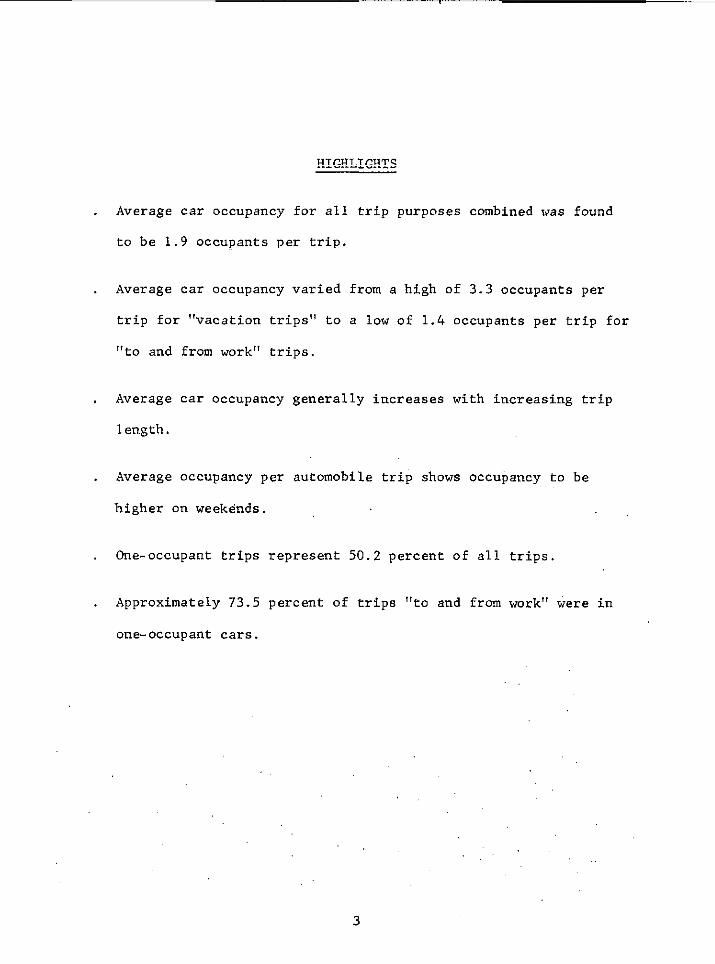
HIGHLIGHTS

Average car occupancy for all trip purposes combinedwas found

to be 1.9 occupants per trip.

Average car occupancyvaried from a high of 3.3 occupants per

trip for “vacation trips” to a low of 1.4 occupantsper trip for

“to and

Average

length.

Average

from work” trips.

car occupancy

occupancy per

“higheron weekends.

Gne-occupanttrips

Approximately73.5

one-occupantcars.

generally increaseswith increasingtrip

automobiletrip ahowa occupancy to be

represent 50.2 percent of all trips.

,,to and from work” Were ‘npercent of trips

3

BACKGROUNDAND PROCEDURES

Background

The Nationwide Personal TransportationSurvey was designed to obtainup-to-date informationon national patterns of travel. Earlier surveys,limited primarily to automobileand truck travel,were conducted in anumber of States between 1930 and 1940 and pore recentlybetween 1951and 1959. In April 1961, a survey was conducted to determine on anational basis characteristicsof travel and ownershipand use of auto-mobiles. In addition, in this national survey in 1961, family incomedata were availablewhich could be related to travel patterns.

Survey procedures

Data for the NationwidePersonal TransportationSurvey were collectedin 1969-1970by the Bureau of the Census of the Departmentof Connnercefor the Federal Highway Administrationof the Departmentof Transporta-tion.

tie survey was based on a multi-stage probabilitysample of housing unitslocated in 235 sample areas, comprising485 counties and independentcities, representingevery State and the District of Columbia. The 235sample areas were selected by grouping all the Nation’s countiesandindependentcities into about 1,900 primary sample units (PSU’S)andfurther forming 235 strata of one or more ?SU’S that are relativelyhomogeneousaccording to socio-economiccharacteristics. With eachof the strata, a single PSU was selected to represent the stratum.Within each PSU, a probabilitysample of housing units was selected torepresent the civilian non-institutionalizedpopulation.

The households in the NationwidePersonal TransportationSurvey com-prised two outgoing panels in the QuarterlyHousing Survey (QHS)conductedby the Bureau of the Census. One panel was interviewedinApril, July, and October 1969, and January 1970; the second panel wasinterviewedonly once in August 1969.

Experiencedfield staff of the Bureau of the Census were assigned tothe survey. Training consisted of a one-day session for,fieldsuper-visor by Washington office personnel,and a one-day session of trainingof the interviewersby field supervisors. In addition, interviewerswere assigned home-study exercises to be turned in befOre each interviewperiod. The interviewerswere also observed periodicallyby field officepersonnel.

The completedquestionnaireswere edited first in the Census regionalfield offices to clear up inconsistenciesand omisaionsand later inthe Washington office. The questionnaireswere then edited, coded,etc., before being put on tapes. Edited tapes for each month of the

I

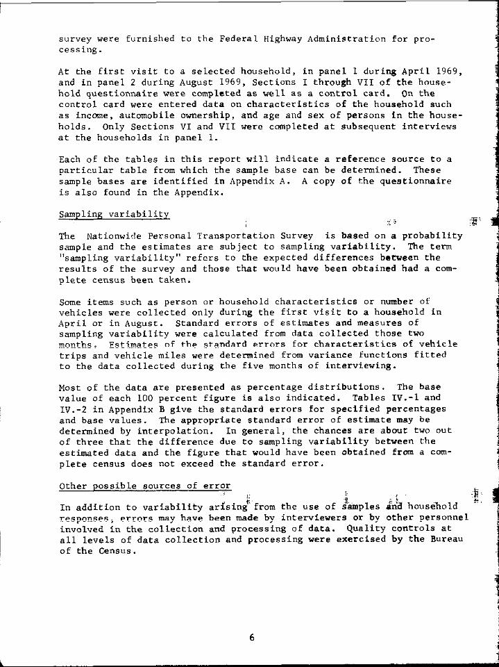
survey were furnishedto the Federa1 Highway Administrationfor pro-cessing.

At the first visit to a selectedhousehold, in panel 1 during April 1969,and in panel 2 during August 1969, Sections I through VII of the house-hold questionnairewere completedas well as a control card. On thecontrol card were entered data on characteristicsof the household suchas income,autmobile ownership,and age and sex of persons in the house-holds. Only Sections VI and VII were cmpleted at subsequentinterviewsat the households in panel 1.

Each of the tables in this report will indicatea reference source to aparticulartable from which the smple base can be detemined. Thesesample bases are identifiedin Appendix A. A copy of the questionnaireis also found in the Appendix.

Sampling variability

me NationwidePersonalTransportationSurvey is based ona probabilitysample and the estimatesare subject to sampling variability. The term“samplingvariability”refers to the expected differencesbetween theresults of the survey and those that would have been obtained had a com-plete census been taken.

Some itas such as person or household characteristicsor number ofvehicleswere collectedonly during the first visit to a household inApril or in August. Standard errors of estimatesand meas”res ofsampling variabilitywere calculatedfrom data collectedthose twomonths. Estimates of the standarderrors for characteristicsof vehicletrips and vehicle miles were determined from variance functionsfittedto the data collectedduring the five months of interviewing.

Most of the data are presentedas percentagedistributions. The basevalue of each 100 percent figure is also indicated. Tables IV.-l andIv.-2 in Appendix B give the standarderrors for specifiedpercentagesand base values. The appropriatestandard error of estimatemay bedeterminedby interpolation. In general, the chances are about two outof three that the differencedue to samplingvariabilitybetween theestimated data and the figure that would have been obtained frm a com-plete census does not exceed the standard error.

Other possible sources of error

Q“ality..co”trol$at EIn addition to variabilityarfsingi’fromthe use of $tiples ~~~ householdresponses,errorsIMY have been made by interviewersor by other personnelinvolved in the collectionand processingof data.all levels of data collectionand processingwere exercisedby the Bureauof the Census.

6

CHAWCTERISTICS OF OCCUPANCY RATES

Occupancy by purpose

In this survey the occupancy for ali purposes (all places and areas cm-bined) was found to be 1.9 occupants per trip (see table 1 and figure 1).The occupancy per trip of the four primary purpose divisionsvaried froma high of 2.5 for ,,~ocialand recreational~~and “educational,civic, and

religious” purposes, to a low of 1.4 occupantsper trip for “earningaliving“ trips. The high for any one subdivisionwas 3.3 occupantspertrip for “vacation,,trips, wile the IOW was 1.4 for trips made “tO and

from work.”

Occupancyweighted by passenger-milesand vehicle-mileswas also computed.The occupancy in passenger-milesper vehicle-mile for “all purposes”was2.2 (see table 1). ‘1’nehighest occupancy for a primary divisionwas 2.9passenger-milesper vehicle-milefor “social and recreational”trips,and the lowestwas 1.6 for trips related to “earninga living.” Valuesfor the purpose subdivisionsranged from 3.3 passenger-milesper vehicle-mile for “vacation trips” to 1.6 for “to and from work” trips.

Occupsncyby population group and purpose

Generally, occupancy of automobilesseemed to be slightlyhigher in unin-corporatedareas than in incorporatedplaces. These data are shown intable 1. Residents of unincorporatedareas reported 2.0 occupants pertrip for trips for “all purposes” cmbined. me correspondingaveragefor incorporatedplaces was 1.9 occupants per trip. Interestingly,occupancyweighted by passenger-milesper vehicle-milewas equal in bothincorporatedand unincorporatedareas at 2.2.

The major exception to this general relationshipwas in the category of“social and recreational”trips. Excluding “vacation”trips, which werea small percentage of the total trips, occupancy in incorporatedplaceswas higher than or equal to occupancy in unincorporatedareas. Thelargest differencewas in “pleasure”trips where incorporatedoutrankedunincorporated2.8 to 2.5 occupants per trip.

TWO other points should be noted. First, occupants per trip for the“family business” category averaged nearly 2.0 for all subdivisions.Secondly,some of the minor differencesbetween the averagesmay be dueto sampling variabilityrather than any real difference in occupancyrates.

Occupancy by SMSA and purpose

Table 2 shows the average occupancy for trips by the residents of thevarious standardmetropolitanstatisticalarea (SMSA) size groupings.Generally, there appears to be no clear relationshipbetween SMSA sizeand occupantsper trip for any given trip purpose.

7

**-’4.

——

——.—*-.

.-’

———

8

0u“

10

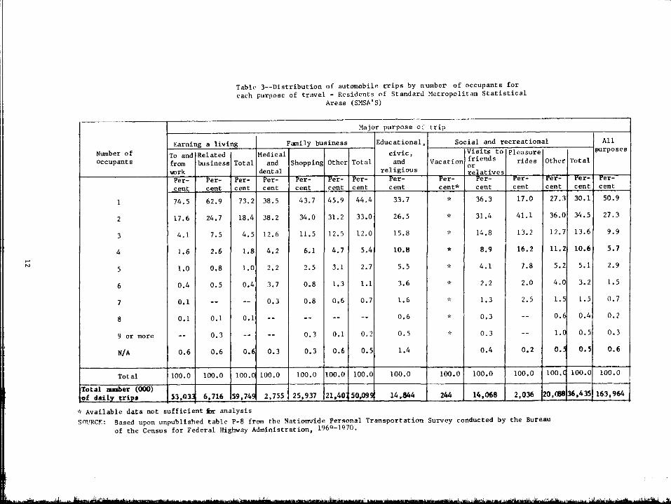
The highest proportionof single occupant cars were for trips “to andfrom work.” As can be seen from table 3, nearly three-fourths(74.5percent) of all “to and from work” trips are made in a single occupantcar. ~en in the “familybusiness” category,which averagea 2.0 occu-pants per trip, over 40 percent of the trips are made by cars with driveronly. It is not surprisingthat over 50 percent of all trips made byresidentsof SkiSA’sare made by automobileswith only one occupant.Furthermore,78.2 percent of all trips made by residents of SMSA’S aremade with only one or two occupants.

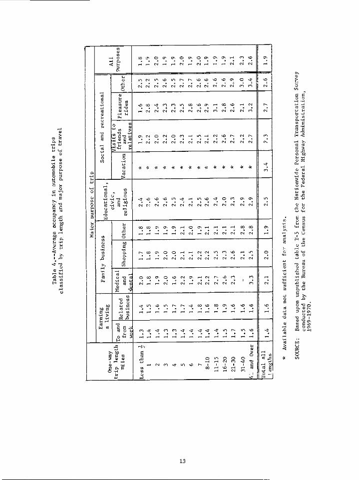
Occupancyby length of trip and purpose

From table 4, occupancyby trip length and purpose, automobileoccupancyaPFe- to generally increasewith increasingtrip length, particularlyfor the longer trips. Although occupancyrates may indeed increasewithincreasinglength in the range less than 15 miles, the figures in table 4do not clearly indicate such a relationship. Further, in some categories,no specificrelationshipcan be seen at all; for instance “educational,civic, and religious”trips.

One categorywhich ahowa a correspondencebetween trip length and occu-pancy is “shopping”trips. The occupancy increaaes from a low of 1.7occupantsper trip for trips less than one-halfmile to more than 2.2occupantsper trip for trips over 10 miles.

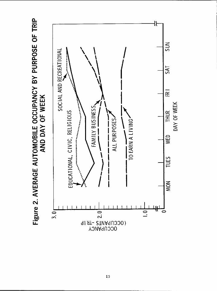
Occupancyby day of week and purpose

Figures taken from table 5, average occupancyper automobiletrip by dayof week and purpose, show occupancy to be higher on the weekends (seefigure 2). For “all purposes,”occupantsper trip vary from a low of1.8 d)lringearly and mid-week to a high of 2.4 on Sunday. In fact, theoccupancyrate increasesfrom 1.8 occupantsper trip on ~ursday, to1.9 occupantsper trip on Friday, to 2.1 on Saturday,and to the highof 2.4 on Sunday.

There are two notable exception to this general relationship. “To andfrom work” trips do not show a clear relationshipto the day of the week.Secondly,“shopping”trips show a relativelyconstant occupancyrate of2.0 occupants per trip for all days of the week.

“Social and recreational”trips generally show a higher weekend occupancyrate in relation to mid-week rates. Occupancy for “viaits to friends and~elati”e~,,trips range from a Wednesday low of 2.O OCCuPantSPer triP t“a Sundayhigh of 2.6.

Table 6 shows the distributionof total trips for each purpose by day ofthe week. As may be seen, most high occupancy trips tend to be taken onthe weekend. For example,“educational,civic, and religioua”tripsshow an all-week average of 2.5 occupantsper trip (table5). It can beseen that over 30 percent of these trips are taken on Sunday alone (table6).

11

Nmber ofoccupants

1

2

3

h

5

6

7

8

9 or more

NIA

Total

.tal be. (mm)

Table 3--DistYib.ti0ll .f a.t.onwbile Wips by numbe~ of occupants foreach Furpose of travel - Residents of standard b[etr.p.lltan Statistical

Areas (SMSA’S)

Major purpose OC trip

Earning a living Fmily business Educational, Social and recreational All

TO and Related Medical civic, Visits t. plea, ”,, ~rp.ses

from business Total and Shopping Other Total and Vacation ~;icnds rides Other Total

wrk dental religious

Per-xelatives

Per- Per- Per- Per- Pel-- Per- per- Per- Per- Per- Per- Fer- rer-cent cent cent cent cent cent cent cent cent+ cent ce”t cent cent ce”t

74.5 62.9 73.2 38.5 43.7 45.9 44.4 33.7 * 36.3 17.0 27.3 30.1 50.9

17.6 24.7 18.4 38.2 M.o 31.2 33.0 26.5 ,< 31. L 41.1 36.0 34.5 27.3

4.1 7.5 4.5 12.6 11.5 12..7 12.0 15,8 l&.8 13.2 12.7 13.6 9.9

1.6 2.6 1.8 4.2 6.1 4.7 5.4 10. II * 8.9 16.2 11.2 10.6 5.7

1,0 0.8 1.0 2.2 2.5 3.1 2.7 5.5 * &.1 7.8 5.2 5.1 2.9

0.4 0.5 0.4 3.7 0.8 1.3 1.1 3.6 * 2.2 2.0 4.0 3.2 1.5

0.1 -- -- 0.3 0.8 0.6 0.7 1.6 *,- 1.3 2.5 1.5 1.5 0.7

0.1 0.1 0.1 -- -- -- -- 0.6 0,3 -- 0.6 0.4 0.2

-- 0.3 -- -- 0.3 0.1 0.2 0,5 .,, 0.3 -- 1.0 0.5 0.3

0.6 0.6 0.6 0.3 0.3 0.6 0.5 1.4 0.4 0.2 0.9 0.5 0.6

100.0 100.0 100.0 100.0 100.0 100.0 100.0 100.0 Im. o 100.0 100.0 100. C 100.0 100.0

. . .f daiLy trips I 53,03~ 6,716 159,744 2,735 I 25,937 121,40~ 50@~ 14,$44 I 244 1 14,068 I 2,036 [20, ~136,4331 163,964

$1Available data not s. fficie”t ti a“alysis

Snl!RCE: 8ased up.” unpublished table P-8 frm the Natior?.ide Personal Transportation Suwey conducted by the 8.rea.of the Census for Federal Nighway Administration, 1969-1070.

.,,,, k

—

—

.m“

—m+“—

om“

—

13

Table 5.--erase!c! OCCUI,.. CY i. a.,.m.bil. tr<P,1,Y purpose of tri? z).<! da) of week

Major purpose of trip

Earning a Iivi”g FamilY bc,siness Educational ,Day of

4

Social a.d recreatid..l

civic,C;,~~d ~e~e~e~ Medical visits to ~,ea,ure All

weekbusiness ‘0”1 de:;:, ‘h”~p”g 0’1”” ‘“’a’ and vacation f’:;’” ,ide$ Other Total ‘rPoses 1

work religl.us relatives ~

Monday 1.4 1.6 1.4 2.0 2.0 2.0 2.0 2.1 * 2.3 3.1 2.4 2.4 1.8

Tue.day I.& 1,5 1.4 2.2 1.8 1.8 1.9 ‘ 2.5 * 2.1 . . 2.1 71.8

Wednesday 1.4 1.5 I.& 2.2 1.9 1.9 2.0 2.5 ,? 2.0 I :.: :.: ,.3 ,,, ~

Thursday 1.4 1.6 1.5 2.1 2.0 1.9 2.0 Z.k * 2.1 2.5 2.32“3 I ’“8

Friday 1.5 1.5 1.5 1.8 2.0 1.8 1.9 2.5 >, 2,1 2.3 2.8 2.5 1.9

Sat. rdav 1.4 1.9 1.5 2.3 2.0 1.9 2.0 2.7 + 2.4 2.8 2.7 2.6 2.1

Sunday 1.3 1,9 1.4 2.4 2.1 2.2 2.1 ?.7 2.6 2.8 2.7 2.7 ~ ,.4—

TotalE21*Y.

1.4 1.6 1.5 2.1 2.0 1.9 2.0 2.5 3.3 2.3 2.7 2.6 2.5 1.9 1

J

:: Available data not sufficient for a..l,, sis.

SOLWE: Based upon unpublishedcable T-7 fro. the Nationwide Personal Tra.sporcatio. Survey conducted by theBureau of the census for tl,e 7.<reral!Iish..j,Admi.istr.tfo., 196’J-197Q.

/

I I I I I I I I I 1’ I I I I I I i If0 0m“ —

di 81- SlNVdf1330)A3NVdf1330

15

——

16

“To and from work” trips show the opposite relationship. This subdivisionhas a low all-week average of 1.4 occupantsper trip. Only 2.8 percent ofthis type of trip is taken on Sunday; the major portion being taken Mondsythrough Friday. Table 7 shows the distributionof total trips for eachday by the purpose of the trip. On Sunday,42.5 percent of the totalnmber of trips are in the high occupancy group, “social and recreational!(2.7 occupants per trip); while on Wednesday,45 percent of the trips arein a much lower occupancy group, ‘learninga living,!!(1.4 occupants pertrip).

Occupancy by time of day and purpose

Shown on table 8 are average occupancies for three selected purposes and“all purposes”by the time of day that the trip was started. The threeselected purposes are “to and from work,” !Ishopping,!(and ‘!vi~itt.friends or relatives.’!These purposes were singled out because of theirparticular importanceby reason of the greatest share of trips. It shouldbe noted that the category ‘all purposestiincludes all trip purposes inthe survey.

Perhaps the most interestingsubdivisionis “to and from work!!trips. Ascan be seen, occupancy decreases steadily from 1.7 occupants per trip at5:00 a.m. to 1.3 occupants per trip at 8:OO a.m. Occ”pancy then holdsrelatively steady until 3:00 p.m. when it jumps to 1.6 occupants per tripIt then decreases again to 1.3 occupants per trip at 6:oO p.m. and holdsfairly constant until 1:00 a.m.

“Shopping” trips display a somewhat different tendencywith time; increasingfrom 1.7 occupants per trip at 8:00 a.m., to 2.1 occupants per trip at 3:00p.m. It appears that the occupancy rate again cycles, going from 1.9occupants per trip at 4:00 p.m. to 2.3 at 8:00 p.m. before it begins tofall off.

Interestingly,the “visits to friends and relati”es” occupancy rates arenot affectedby time of the day. Although occupancy rates are slightlyhigher after 8:00 p.m., most occupancy rates hover around the 24-houraverage of 2.3 occupants per trip.

“All purposes” trips display much the same tendency. The times of lowestoccupancy are from 4:00 a.m. to 8:00 a.m. The times of highest occupancyaPPear tO be from 6:00 p.m. to 11:00 p.m. It seems, however, that onlyin a few cases is the actual ho”rly occ”pancy far from the 24-hour averageof 1.9 occupants per trip.

Distributionof one occupant trips by purpose and hour of the day

Table 9 and figure 3 show the percent of all trips taken in one-occupantcars for a given purpose and time. The one-occupanttrips represent50.2 percent of all trips. As might be expected,73.5 percent of trips“to and from work” were in one-occupantcars. On the other end are“visits to friends or relatives”with 36.3 percent being one-occupanttrips.

17

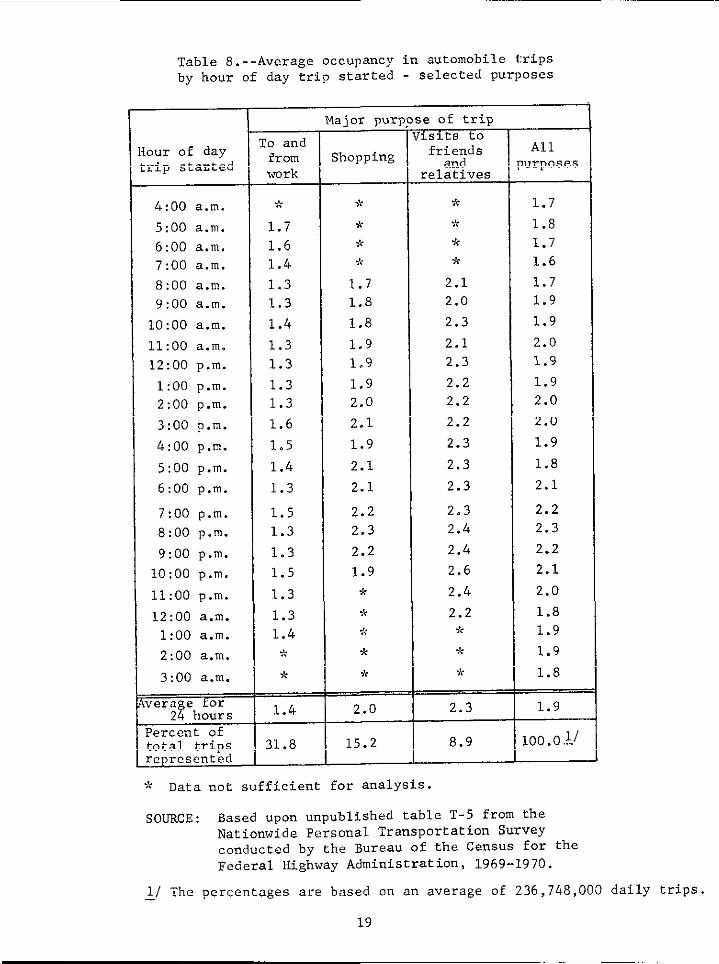
Table 8.--Averageoccupancy in automobiletripsby hour of day trip started - selected purposes

our of dayrip started

4:00 a.m.

5:00 a.m.

6:00 a.m.7:00 a.m.

8:00 a.m.

9:00 a.m.

10:00 a.m.

11:00 a.m.

12:00 p.m.

1:00 p.m.2:00 p.m.

3:00 p.m.

4:00 p.m.

5:00 p.m.

6:00 p.m.

7:00 p.m.

8:00 p.m.

9:00 p.m.

10:00 p.m.

11:00 p.m.

12:00 a.m.1:00 a.m.

2:00 a.m.

3:00 a.m.

?eragetor24 hours

‘erccntof:otaltripsrepresented

ro and?romwork

,.,

1.71.61.4

1.31.3

1.4

1.3

1.3

1.31.3

1.6

1.5

1.4

1.3

1.51.3

1.3

1.5

1.3

1.31.4,,>.

*

1.4

31.8

Major pur

Shopping

9<

%

>k

;,

1.71.8

1.8

1.91.9

1.92.0

2.1

1.9

2.1

2.1

2.22.3

2.2

1.9J<>!,

!:-

*,,,

2.0

15.2

e of trip

q

Lslts to

friendsand

relatives

*

*

*;,

2.12.0

2.3

2.12.3

2.22.2

2.2

2.3

2.3

2.3

2.32.4

2.4

2.6

2.4 I2.2+<

*

*

2.3

8.9

Alllurposes

1.7

1.81.71.6

1.71.9

1.9

2.01.9

1.92.0

2.0

1.9

1.8

2.1

2.22.3

2.2

2.1

2.0

1.81.9

1.9

1.8

1.9

100.01/

* Data not sufficientfor analysis.

SOURCE: Based upon unpublished table T-5 from theNationwidePersonal TransportationSurveyconducted by the Bureau of the Census fOr theFederal Highway AdministratiOn,1969-1970.

:/ The percentagesare based on an average of 236,748,000daily trips.

19

Table 9.--Proportionof trips in one-occupantautomobilesby hour of day trip started - selected purposes

Hour of daytrip started

4:00 a.m.

5:00 a.m.

6:OO a.m.

7:00 a.m.

8:00 a.m.

9:00 a.m.

10:00 a.m.

11:00 a.m.

12:00 p.m.

1:00 p.m.

2:00 p.m.

3:00 p.m.4:00 p.m.

5:00 p.m.6:00 p.m.

7:00 p.m.

8:00 p.m.

9:00 p.m.

10:00 p.m.

11:00 p.m.

12:00 a.m.1:00 a.m.

2:00 a.m.

3:00 a.m.

24 Hours

To andfromwork

T

68.3

65.1

74.4

77.4

78.0

78.082.0

79.7

78.378.1

64.969.1

75.678.5

71.2

78.8

76.5

71.1

76.0

81.066.9*

*

73.5

Major purl

Shopping

~ ;!:

*

*

J<

54.6

49.4

50.647.5

48.1

41.839.8

41.147.1

43.244.6

34.1

31.5

33.239.1**

>;-

*,!,.

43.3

Ieof tripvisits tofr~~ds

relativesPer$ent

*

+:

$,

45.1

47.7

43.345.3

36.8

38.238.4

40.938.3

35.235.3

38.2

27.9

27.823.1

38.1

42.6*

i-

*

36.3

Allpurposes

‘etL?t

64.3

61.6

65.4

59.9

53.7

49.349.2

51.3

50.048.3

47.354.0

55.145.3

36.5

35.0

37.740.1

45.0

53.939.3

51.6

43.8

—

50.2

* Data not sufficientfor analysis.

SOURCE: Based upon unpublishedtable T-5 from theNationwidePersonalTransportationSurveyconductedby the Bureau of the Census for theFederal Highway Administration,1969-1970.

20

,... -J..

——f I

I

Jb

J,/

I I

(Sdl811V101 40 lN20M3d)Sdl Ml 311HOWOIIIV lNVdf1300-3N0

21

The “all purposes” one-occupantcar percentagesare above the averageduring both morning and e“ening “rushrthours (6:00~.m, t. 9:013a.m. and3:00 p.m. to 6:OO p.m., respectively)when “to and frm work!!trips exerttheir largest influence. Ouring the eveninghours of 6:00 to 11:00 p.m.,however, “all purposes” percentages drop below the 24-hour average to alow of 35.0 percent being one-occupanttrips. Perhaps this representsthe greater influenceof “shopping!’and “visits to friends or relatives”trips. It is interestingthat during these same hours, only percentagesfor “to and frm work” trips do not drop. It should be remembered thatas one-occupanttrip percentagesdecrease the autunobile occupancygenerally increases. ~is can be seen from tables 8 and 9 where the “allpurposes” percentage is the lowest (35.0percent) for trips started at8:00 p.m. This low percentagecorrespondsto the “all purposes” occu-pancy high of 2.3 occupantsper trip.

22

SWRY

1. Occupancy rates of passenger cars are affected by the purpose

of the trip. It seems that purposes that encourage family activity suchas “social and recreational,,trips d. in fact result in higher OccuPancY

rates. On the other hand, trips which a single familymember might take,such aS Iptoand from work,11d. re~~lt in 10Wer Occupancy ‘ates.

2. me size of the standardmetropolitanstatisticalarea has noclear relationshipto occupancy rates. Although there does appear tobe sme differencebetween incorporatedplaces and unincorporatedareas,this differencemay be due to statisticalvariance.

3. Length of trip, day of week, and time of day all have some affecton automobileoccupancy rates. It is difficult to see, however, if theydirectly influenceoccupancy rates or, if they affect the type or purposeof the trip. Even though it can be seen that these variables do influenceoccupancyrates for individualpurposes, it is probably true that ‘highoccupancy!,~rip~ ~re ~nco”ragedby the above variables tO an even greater

extent.

4. Although the “all purposen average is near 2 occupantsper trip,nearly 50 percent of all trips are still taken in one-occupantcars.Even when occupancy approaches 3.0 occupantsper trip, the percent of one-occupamt cars is still high. It is noteworthy that nearly three-fourthsof =11 trips taken ,Itoand from!!work are taken in one-occupant,driveronly, cars.

23

APPENDIXA

Sample base for Nationwide Personal TransportationSurvey

The followingare the major series of tables and the sample base fortables developed from the survey. Each of the tables in any of these re-ports will indicate a reference source from which the sample base can bedetermined.

1. –H-series,j-series, and T-9 through2-16—

These tables relate to data collected in SectionsI throughv of the questionnaire. The tables are based upon a sampleof approximately6,000 households,approximately3,000 frompanel 1 intervie~tedin April 1969, and approximately3,000from panel 2 interviet.edin August 1969. Each of thesepanels were expanded to national estimates. For purposesof all tables referred to in any of these reports, the ex-panded data from the two panels were averaged.

2. P-series and T-1 through T-8— —

These tables relate to data collected in Section VI. Datafrom four interviewsat the identicalhouseholds in panel 1(approximately3,000 householdswere interviewedin April,July, October 1969, and January 1970) were combined and ex-panded to represent annual estimatesof trips and travel byautomobileor other forms of public tranaportation.

25

APPENDIX A

Major sectionsof questionnaire

The followingare the main sectionsof the questionnaire:

1. The data reported in items a through t above Section 1 ofthe questionnairewere transcribedfrom the control card.

2. SectionI - AutomobileRecord

3. Section II - Shoppingand nearness to public transportationto main business districtby residentsof Standardiletro-politan StatisticalAreas.

4. Section 111 - Travel to work for all mployed persons 16years or older.

5, Section IV - Driver informationor estimatedannual milesdriven by licensed drivers.

6. Sectionv - Travel to school for persons between 5 and 18years of age and attending school. For panel 2 of thehouseholdsinterviewedin August 1969, the interviewerasked for the travel to school informationfor the pre-ceding May.

7. SectionVI - Travel day report. All one-way trips bymotor vehicle or some fom of public transportationtakenby persons 5 years of age or older were reported for apre-assignedreferenceday. The referenced~s were allin a one-weekperiod in each of the months of interviewingand all weekdays and weekendswere represented. Generally,the interviewervisited all households the first weekdayafter the referenceday in order to minimize mmory errors.

8. SectionVII - Overnighttravel record of all trips lastingone or more nights during the 7 days ending the day beforethe preassignedtravel day. Insufficientdata were col-lected in this section to permit detailed analyses.

26

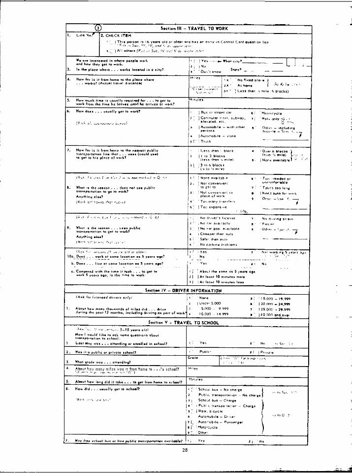
(3) S.c,i.. 111. TRAVEL TO WORK

.

-. 4

,. w,., ..,...6 (,. ”,.s .,*d?,,,., ,..,,, ,,, ,,,,,.,.,,, , I------,;-----j------;r--j.---..,:.....-.l .,

..,. i. !,,,. .,.. ,,, ..,? I Numb., I ..m~r I ....-numti, l—N..kr

,.{r,..,ro 12,7Y1*-Al(L!!p$prcvl.”slYreP.r!Qd, ,,,,,,,,”.,,,,.,,,.,..”,.a,,—

29

s..tiom VII . 0vE8MlGHT TRAVEL

1,,, !. I 1.,,2. “— r,,, ,.OUT-U N...,, L,..*. , ,,.. . . .

e ,,.. .., ,

1, “.. . . . . .,,., ,. ,, ,,.”, h... ,. .,’,, M,!.,.,,,. “,..,,

.,,.,(To ‘.,,,.,, ,.,”,,

~ H.. ~“.h ,1~.d,d .P..d ,.”,m,~.r.,(,.,., !,,”. ‘,..,.,”. ,. ‘.,,,,,, ,.,.,, . . . [. ) “O”r,

l—, c 1.W,i —! D“o. rs

,.,, ,,..,, ,,”’=} /,.,,. ...,,,,, .,, he., “, ..,, !2 r: .,,, 2 : Ioa, ’ –*n.D., s

3. Wha, ,im. .’rd; d;d ,*. ,,,, ,,..?! r-] ..., , cl ..m.

+Z,r ,,, ”, + —I n...Zn,.m. —~—n....4. 0. h., ,., .! ,h. .,ek did ,,. .,9 ,*,,,

, q~”. $rl ~-s. cl,.”. *C-1 %.. I r7s....II T,.,,.:~ +~~.,6~’1F,!.z~<.m. .! ]P,,.,~w.. ,~, r,,

, 7 :-:5.!. , L ; Tu=%.7 I-!. : [j J:::,, ~s.t,.~jw.d. an ..,.

C.,. K.r — ,, TO -,, 7, “...,,..1, 8.*,, .O,,= . . . ,0 ~,k ,. V,,,, ,,,.,, ., ~,.,,vc,3. S,*,,., ,. P! ”s.,e ,,, $;.,4.0,~ ,..,,, .,,., s..., ,.,,..s, 10. O*, ,..,., ., ,..,..,,.”.,5. T.,ch., ., ...,<, ,,, h,6. T. *.,.,., d..,,,,

T,<, 1 ! ,,,.1 I T*25, Wh’ . . . ,h. ,”., ”,...m ,.r,h, ,,, p? (E”,,,, .*.,

1

c.,. Ke,— ,. SC* I ,“s 7. A.,-.,,,. ..,,..,2. O,t,m b“, .../., ,,,,., ,., B. A.!-,,,. ,.,,..,.,3. ,,.”.,., ., S.,”,., 9, m.!-,.,, ., ..,.,,,,,

$.,gl,::,m::::,y, !,...,.,,.,,.. . . . . “,.0+, 0!.., “a,. \;: :,:: (,..,4,,., ,.,.”,),. A,,,,..,,, T..,

(l.cltie. !!.e.., s“’, ., !,..,,O,,.,,O. 7,,* ,!. .., ,,.. ,erm,,. o,, ., .,,1 ., ..,., I Trip 2 7+2

“,,5.,, ,,:, . ..,., .... s,)

{’, .,,,,, .&e , .,, ,.s b.. ,.,..,, Au!. . . .,.0. . .... !?,, ,.,; ,,.”, 7.., I A.,. .., .“!. N..

7. W,., .W,o”,.b,,e . . . .S.d, -------.; ------4 ---- .-e; -

:Transcr? b.. ”re.. b,le .,, -,., ,,.. C.c. j.

9: ]M., m ..1.,,.,d ~ she,... ‘fi;:::”:”:. c,c, ‘~”::;::;”:c,c,

0, Who,,.,. ,,e,.,...b, ?.? 0!, ”., L, ”.... .f’.ti ,,”, . . . D!,..! ,,.. ..,

(If .Ors ,,.. .,,.,,>.,,, ,.(,, r,,. 1,.. .:,mb,..,,., .,,,.. ., ”,,... ,,, “,. ,, .,,,, , 4

or

I “ ““---- ““ ..:””-” ”, ,c]No, .h.., e..,d ,,~ &.:L:o.,$,d ,,, ; .., .*,*.,,.*.,

9. “.. ..., ...,,. w.- ,.,,, a.,.m.b,,,,i ..,.,,., ...,,,,y”,jrj,:;j:::::::; c,,,d,,. .....5 .:..,,.

,.”.&r N.mkr

,s,”.. m,, -T,<. 1 ,,,, ,I T*S

0. H.. ..., n,,h,, . . . . . . . em, k.m k..? N “ret-r N“”,M, .“”,,,,

2. wk., ,,....,,. ,.,

., --4-091!, - O,,.,,r I

!,,, .

1 I 1,...7.,,1,0, ,... .“, e,d or, ”,, .,., . . . .., ”!, ., ”..., orl..r ., ”.....“,.; =,= .., s,..s ,5 .“. ,,! /“

5.Who,,... ,,. .,,...6,,.?,...--,,...---,

., ““--i- :,-------i

(L!sr 1?.. ...,:?! 0/.,,., ,. ”,4.,,.,.6.,5 I I I I I I I5 “..rs old .r., d=, .h” .“. ”,”. ,,,5 .o..d ,,,.)

[I I 1 I I I I I I

w

APPENOUB

Table IV.-l.--Estimatedstandarderrors for numberofvehicle trips for one day when

singleauto is only means

Estimatedtotal(000)

100

250

500

750

1,000

2,500

5,000

10,000

15,0,00

25,000

50,000

75,000

100,000

125,000

150,000

175,000

200,000

225,000

235,000

255,000

Estimatedstandard(1 Sigma)(000)

error

95

150

213

261

302

479

683

982

1,222

1,625

2,459

3,197

3,893

4,567

5,228

5,879

6,524

7,164

7,420

7,802

These standarderrorsmay be used to evaluatethe percentagesshown in tables3, 6, 7, and 9.

31

APPENDIX B

Table IV.-2.--Estimatedstandard errors for percentagesof

Base ofPercentage

(000)

500

750

1,000

2,500

5,000

10,000

15,000

25,000

50,000

75,000

100,000

125,000

150,000

175,000

200,000

225,000

235,000

255,000

vehicle trips for one day whensingle auto is only mea”s

,$ .

1 of 99%

1.3

.9

.8

.6

.4

.3

.3

.3

.2

.2

.2

.2

.2

.2

50T95X

4.1

2.9

2.1

1.7

1.3

.9

.8

.7

.6

.5

.5

.4

.4

.4

.4

I

Estimatedpercentage

10 or 90%

10.4

9.0

5.7

4.0

2.9

2.3

1.8

1.3

1.Q

.9

.8

.7

.7

.6

.6

.6

.6

20 or 80-

17.0

13.9

12.0

7.6

5.4

3.8

3.1

2.4

1.7

1.4

1.2

1.1

1.0

.9

.8

.8

.8

.8

I

25 or 75%

18.4

15.0

13.0

8.2

5.8

4.1

3.4

2.6

1.8

1.5

1.3

1.2

1.1

1.0

.9

.9

.8

.8

50%

21.2

17.3

15.0

9.5

6.7

4.8

3.9

3.0

2.1

1.7

1.5

1.3

1.2

1.1

1.1

1.0

1.0

.9

These standard errorsmay be used to evaluate the percentagesshownin tables 3, 6, 7, and 9.

32

,.0 ,,,.,24