Nationwide Analysis of U.S. Commercial Building Solar Photovoltaic

NREL is a national laboratory of the U.S. Department of Energy Office of Energy Efficiency & Renewable Energy Operated by the Alliance for Sustainable Energy, LLC This report is available at no cost from the National Renewable Energy Laboratory (NREL) at www.nrel.gov/publications.

Contract No. DE-AC36-08GO28308

Nationwide Analysis of U.S. Commercial Building Solar Photovoltaic (PV) Breakeven Conditions Carolyn Davidson, Pieter Gagnon, Paul Denholm, and Robert Margolis National Renewable Energy Laboratory

Technical Report NREL/TP-6A20-64793 October 2015

NREL is a national laboratory of the U.S. Department of Energy Office of Energy Efficiency & Renewable Energy Operated by the Alliance for Sustainable Energy, LLC This report is available at no cost from the National Renewable Energy Laboratory (NREL) at www.nrel.gov/publications.

Contract No. DE-AC36-08GO28308

National Renewable Energy Laboratory 15013 Denver West Parkway Golden, CO 80401 303-275-3000 • www.nrel.gov

Nationwide Analysis of U.S. Commercial Building Solar Photovoltaic (PV) Breakeven Conditions Carolyn Davidson, Pieter Gagnon, Paul Denholm, and Robert Margolis National Renewable Energy Laboratory

Prepared under Task No. SS13.1040

Technical Report NREL/TP-6A20-64793 October 2015

NOTICE

This report was prepared as an account of work sponsored by an agency of the United States government. Neither the United States government nor any agency thereof, nor any of their employees, makes any warranty, express or implied, or assumes any legal liability or responsibility for the accuracy, completeness, or usefulness of any information, apparatus, product, or process disclosed, or represents that its use would not infringe privately owned rights. Reference herein to any specific commercial product, process, or service by trade name, trademark, manufacturer, or otherwise does not necessarily constitute or imply its endorsement, recommendation, or favoring by the United States government or any agency thereof. The views and opinions of authors expressed herein do not necessarily state or reflect those of the United States government or any agency thereof.

This report is available at no cost from the National Renewable Energy Laboratory (NREL) at www.nrel.gov/publications.

Available electronically at SciTech Connect http:/www.osti.gov/scitech

Available for a processing fee to U.S. Department of Energy and its contractors, in paper, from:

U.S. Department of Energy Office of Scientific and Technical Information P.O. Box 62 Oak Ridge, TN 37831-0062 OSTI http://www.osti.gov Phone: 865.576.8401 Fax: 865.576.5728 Email: [email protected]

Available for sale to the public, in paper, from:

U.S. Department of Commerce National Technical Information Service 5301 Shawnee Road Alexandria, VA 22312 NTIS http://www.ntis.gov Phone: 800.553.6847 or 703.605.6000 Fax: 703.605.6900 Email: [email protected]

Cover Photos by Dennis Schroeder: (left to right) NREL 26173, NREL 18302, NREL 19758, NREL 29642, NREL 19795.

NREL prints on paper that contains recycled content.

http://www.osti.gov/scitech

http://www.osti.gov/

mailto:[email protected]

http://www.ntis.gov/

mailto:[email protected]

iii This report is available at no cost from the National Renewable Energy Laboratory (NREL) at www.nrel.gov/publications.

Acknowledgments This work was made possible by the Solar Energy Technologies Program at the U.S. Department of Energy (DOE). The authors wish to thank Sean Ong, Clinton Campbell, Nate Clark, Peter Jeavons, Billy Roberts, and Angela Crooks for their contributions in developing and refining the framework for this analysis as well as Galen Barbose, Laura Vimmerstedt, Shanti Pless, and Jarett Zuboy for providing review and feedback.

iv This report is available at no cost from the National Renewable Energy Laboratory (NREL) at www.nrel.gov/publications.

List of Acronyms CBECS Commercial Building Energy Consumption Survey DOE U.S. Department of Energy DSIRE Database of State Incentives for Renewables &

Efficiency EIA U.S. Energy Information Administration ITC Investment Tax Credit kW kilowatt kWh Kilowatt-hour MACRS Modified Accelerated Cost Recovery System NREL National Renewable Energy Laboratory PPA Power-purchase agreement SAM System Advisor Model SREC Solar renewable energy credit TMY3 Typical Meteorological Year 3 TOU Time of use W Watt

v This report is available at no cost from the National Renewable Energy Laboratory (NREL) at www.nrel.gov/publications.

Executive Summary The commercial sector offers strong potential for solar photovoltaics (PV) owing to abundant available roof space suitable for PV and the opportunity to offset the sector’s substantial retail electricity purchases. However, the sector includes a wide variety of building end uses and occupancy/ownership structures, which challenges the ability to scale-up PV deployment. Broad-scale financial analysis of commercial PV is complicated by the fact that commercial retail rates are complex and vary substantially across utilities.

In this report we evaluate the breakeven price of PV for 15 different building types by calculating electricity savings based on detailed rate structures for most U.S. utility territories (representing approximately two thirds of U.S. commercial customers). We evaluate breakeven prices assuming several financing options: cash purchase, loan and PPA. We also explore breakeven pricing under the current 30% federal Investment Tax Credit (ITC) as well as a reduced 10% ITC case. In all scenarios we exclude additional state or utility incentives. Major findings from the analysis include:

• Breakeven prices nationwide exhibit substantial variation based on widely varying retail rate tariffs. In the cash purchase with 30% ITC case, the median breakeven price, for an ‘average’ building—for all states and Washington, D.C. but not Hawaii—ranges from $0.80/W to $3.20/W. At a PV capital cost of $1.67/W, half of all commercial customers would break even.

• In the cash purchase with 30% ITC scenario, in most, but not all, utilities, commercial PV does not achieve break even given current commercial PV capital cost estimates of $2.17/W (without state or utility incentives). In the 1,355 utilities modeled, an estimated 32% of U.S. commercial customers could break even.

• Loan financing that distributes payments over the life of the PV system significantly increases the fraction of commercial customers that could break even relative to the cash purchase scenario. In the 4.9% loan with 30% ITC case, the percentage of commercial customers that break even given current installed costs approximately doubles to 64%.

• In both the cash purchase scenario and the loan scenario, reducing the federal ITC from 30% to 10% decreases the fraction of commercial customers achieving break even at current costs by approximately half.

• At the U.S. Department of Energy SunShot target of $1.37/W in 2015 dollars (stated target was $1.25 in 2010 dollars ) an estimated 66% of commercial customers for all building types break even under a 30% ITC cash purchase scenario, and 45% break even under a 10% ITC scenario. The loan scenario, again, provides much more favorable conditions with an estimated 89% of commercial customers achieving breakeven conditions under a 30% ITC and 66% under a 10% ITC scenario.

• Variation in retail rates is a stronger driver of breakeven prices than is variation in building load or solar generation profiles.

vi This report is available at no cost from the National Renewable Energy Laboratory (NREL) at www.nrel.gov/publications.

Even though the breakeven price of a particular building is most strongly driven by the local utility rates, the breakeven price is moderately impacted by building end use as well. Our analysis suggests the following results:

• Variation of the average breakeven price between building types is largely a function of the ability of PV to reduce demand charges for the given building types. Buildings whose peak load occurs during daylight hours (e.g., offices and schools) tend to see a greater reduction in demand charges, as PV generated electricity has the ability to decrease a building’s daily peak demand. Buildings whose peak load occurs in the evening or night (e.g., hotels and restaurants) tend to see little or no reduction in demand charges, as PV generation does not coincide with the peak load. As demand charges are usually set by a month’s peak demand, a single overcast day coinciding with high energy use can eliminate any potential reductions in demand charges for all building types.

• The value of PV derived from avoided energy charges is more consistent across building types. A PV system offsets a building’s energy consumption the same regardless of the shape of the original load profile. The financial value of this offset electricity is then set by the energy charge of a building’s utility rate, which can vary by building type. For nearly all of the buildings studied, the bill savings from avoided energy charges exceeded the bill savings from reduced demand charges.

The building types with the highest breakeven price, and therefore the highest willingness to pay for a PV system were small offices, warehouses, and schools. The building types with moderate average breakeven prices were retail establishments, medium and large offices, quick-service restaurants, outpatient medical facilities, and supermarkets. The building types with the lowest average breakeven prices were hotels, hospitals, and full service restaurants. Given the variation in breakeven price within building types, individual commercial building owners should evaluate the financial soundness of PV for their building considering local utility rates, incentives, and net-metering regulations.

vii This report is available at no cost from the National Renewable Energy Laboratory (NREL) at www.nrel.gov/publications.

Table of Contents 1 Introduction ........................................................................................................................................... 1 2 Methodology ......................................................................................................................................... 3

2.1 System and Financing Assumptions ................................................................................................. 3 2.2 Solar Resource and Meteorological Data ......................................................................................... 5 2.3 Building Load Data and System Size ............................................................................................... 5 2.4 Utility Rate Data ............................................................................................................................... 8

3 National-Level Results ....................................................................................................................... 11 3.1 Nationwide Average Breakeven Conditions by Utility .................................................................. 11 3.2 Breakeven Price Range by State ..................................................................................................... 14 3.3 Breakeven Price Sensitivity ............................................................................................................ 15

4 Building-Level Results ....................................................................................................................... 18 4.1 PV Systems Effect on a Building’s Monthly Demand Charges ..................................................... 19 4.2 PV Systems Effect on a Building’s Energy Charges ...................................................................... 23 4.3 Breakeven Price Range by Building Type ..................................................................................... 25

5 Conclusion .......................................................................................................................................... 26 References ................................................................................................................................................. 27

viii This report is available at no cost from the National Renewable Energy Laboratory (NREL) at www.nrel.gov/publications.

List of Figures Figure 1. Loads for various building types in winter (January 1) and summer (July 1), Denver ................. 8 Figure 2. PV breakeven prices ($/W) for an average commercial building in the cash-purchase scenario,

2015 (including Federal 30% ITC and MACRS, but no state incentives) ............................. 12 Figure 3. PV breakeven prices ($/W) for an average commercial building in the loan scenario, 2015

(including Federal 30% ITC and MACRS, but no state incentives) ...................................... 12 Figure 4. PV breakeven prices ($/W) for four commercial building types in the cash-purchase scenario,

2015 (including Federal 30% ITC and MACRS, but no state incentives) ............................. 13 Figure 5. Breakeven price ranges by state (except Hawaii) for the average of all building types, 2015

(including Federal 30% ITC and MACRS, but no state incentives) ...................................... 15 Figure 6. Fraction of commercial customers that break even as a function of installed cost under various

scenarios (green area represents costs at or above current PV system price) ........................ 16 Figure 7. Fraction of commercial customers that break even as a function of PPA rates ........................... 17 Figure 8. Load profile of four building types, with and without PV, for a July weekday in Pasadena ...... 19 Figure 9. Change in peak demand at various PV system sizes (as percentages of annual electricity

consumption the system would offset) for a supermarket in Austin on an August weekday 20 Figure 10. Change in peak demand at various PV system sizes (as percentages of annual electricity

consumption the system would offset) for a small hotel in Austin on an August weekday ... 21 Figure 11. August demand charge as a function of annual energy consumption offset by PV for an Austin

supermarket and small hotel under Austin Energy’s commercial rate for buildings inside the city with a demand greater than 50 kW ................................................................................. 22

Figure 12. TMY3 solar resource profile for Hartford for the month of February ....................................... 22 Figure 13. Simulated net-load profile for a small office building in Hartford over 2 days with variable

solar resource (one high day, one low day) ............................................................................ 23 Figure 14. June monthly charges for a supermarket (Austin, commercial inside-city rate), small hotel

(Miami, GSDT-1 rate), full-service restaurant (Seattle, MDD rate), and hospital (Albuquerque, GPS-TOU rate) .............................................................................................. 24

Figure 15. Nationwide breakeven prices by building type ......................................................................... 25 List of Tables Table 1. Modeled PV System Assumptions .................................................................................................. 3 Table 2. Financing Assumptions for cash Purchase, Loan, PPA, and no-ITC Sensitivity Scenarios ........... 4 Table 3. Characteristics of DOE Commercial Reference Buildings ............................................................. 7

1 This report is available at no cost from the National Renewable Energy Laboratory (NREL) at www.nrel.gov/publications.

1 Introduction In the first quarter of 2015, the commercial sector installed approximately 17% of total new U.S. solar photovoltaic (PV) capacity (GTM Research and SEIA 2015a). Yet the commercial sector faces substantial barriers to adopting and scaling-up PV, including a diverse set of stakeholders and submarkets, variety in occupancy and ownership, and a focus on first cost (Feldman and Margolis 2014, Alliance to Save Energy 2013). In fact, growth in new commercial installed PV capacity has remained roughly flat since 2011, while residential- and utility-sector growth continues to accelerate (GTM Research and SEIA 2015b).

The potential for PV in the commercial sector is large; this sector accounts for roughly 36% of U.S. primary energy consumption, and U.S. commercial building electricity demand likely will continue to grow with continued economic growth and demand for commercial services (DOE 2015). Further, many commercial buildings have large, flat roofs suitable for PV systems capable of generating a significant portion of the building’s annual electricity needs: an analysis of Light Detection and Ranging (LiDAR) data in major U.S. cities indicates that more than 99% of commercial-sized buildings have at least one roof plane suitable for PV deployment (Gagnon et al., forthcoming).1

To evaluate the potential of PV for the commercial sector, the business case must first be understood. In the case of distributed generation, this requires evaluating the avoided cost of retail electricity given specific rate tariffs, retail net metering, and coincidence of PV generation with building electricity demand. Rate tariffs and retail net metering vary based on the utility, while building electricity demand varies based on building use, cooling and heating requirements, and many other factors. As a result, characterizing the economic feasibility of PV in the commercial sector can be challenging. The National Renewable Energy Laboratory (NREL) previously analyzed “breakeven prices” (defined below) for residential rooftop PV systems in the United States (Denholm et al. 2009) and evaluated commercial breakeven prices and electricity-rate drivers in limited markets (Ong et al. 2010, Ong et al. 2012) and specific building segments (Ong et al. 2011; Ong et al. 2013). Several analyses have explored the impacts of rate structures and net metering on the economics (Wiser et al. 2007; Darghouth et al. 2013) and deployment (Darghouth et al. 2015) of distributed PV systems in California or nationwide.

This report provides a nationwide snapshot of the economic feasibility of commercial PV across building types by evaluating both cash-purchase and loan financed PV systems in most utility service territories. Economic feasibility is typically considered necessary to move a project forward to installation. Throughout the report, we refer to this concept as the breakeven price: the PV installation price in dollars per watt ($/W) of installed PV system capacity at which the net present benefit of offset grid electricity purchases equals the PV system capital cost, net of both federal incentives and operations and maintenance costs.

The remainder of the report is structured as follows. Section 2 describes our methodology. Section 3 provides high-level breakeven results by geographic location for a cash purchase and loan scenario and compares results with breakeven results from a reduced federal Investment

1 That is, 99% of buildings had at least 10 m2 of contiguous roof space available with a tilt of less than 60 degrees, and a south, east, west, southeast, or southwest azimuth.


Tax Credit (ITC) scenario and a power-purchase agreement (PPA) scenario.2 Section 4 presents results at the individual building level, exploring the effects of PV on building peak demand and energy consumption as well as breakeven prices by building type. Section 5 offers conclusions and directions for future research.

2 These scenarios only cover a very small amount of the actual variation present in commercial financing and incentive capture, but they illustrate high (4.9% loan) and low (reduced ITC) breakeven price cases.


2 Methodology To calculate the breakeven conditions of rooftop PV systems for many utilities, we modeled PV systems in NREL’s System Advisor Model (SAM, version 2015.1.30). SAM is a free, publically available performance and economic model designed to facilitate decision making and analysis for renewable energy projects (Gilman and Dobos 2012). SAM uses hourly meteorological data, a PV performance model, and user-defined assumptions to simulate the technical and financial performance of a PV installation. Relying on a set of SAM scripts, we estimated the breakeven price for 15 different building types in 1,355 utility service territories, representing portions of all 50 states that, in aggregate, serve 66% of all commercial customers in the U.S. We also calculate an average breakeven price by constructing an average of all the building types modeled, weighted by the fraction that each building category contributes to the total national building stock. The following sections document our data sources as well as the technical and financial assumptions made throughout this analysis.

2.1 System and Financing Assumptions The technical parameters of PV systems vary depending on the building parameters and the design choices of the installer. For this analysis, a set of performance assumptions were made to represent a cost-effective system design (Table 1). We used these values in SAM, in conjunction with solar resource and meteorological profiles, to determine the energy production of the PV system.3

Table 1. Modeled PV System Assumptions

Characteristic Value

System Size Building specific (see Section 2.3)

Module Type Multicrystalline silicon

Module Power Density 156 W/m2

Tilt 15 degrees

Azimuth 180 degrees (south facing)

Ground Coverage Ratio 0.65

Total System Losses4 14.08%

Module Degradation 0.75%/year

Inverter Efficiency 95%

DC to AC Ratio 1.4

Financing options vary based on factors including the commercial customer’s credit, capital availability, and business strategy. Most businesses likely would purchase a PV system using a line of business credit, rather than cash, when possible. Some banks have offered PV-specific

3 Documentation of the mathematical models used by SAM is available within the program, under the “Help” section. 4 These are SAM’s default total system losses, which include losses for a distributed commercial PV system related to soiling, shading, snow, mismatch, wiring, connections, light-induced degradation, nameplate, age, and availability.


financing through a capital lease, though this option is currently not widely available. Consequentially, we evaluate both a cash-purchase scenario as well as a loan scenario, including the ITC at the 2015 level of 30%. For the loan scenario, we assume a 4.9% loan rate, which can be considered a relatively optimistic case in contrast with the relatively pessimistic case of the cash purchase scenario. We match the discount rate in all scenarios to the assumed loan rate, assuming that the discount rate reflects the weighted average cost of capital, or the opportunity cost of capital. Naturally, the weighted average cost of capital for a particular business varies extensively depending on the industry, capital stack and many other factors. To characterize the breakeven prices for another common financing mechanism, we also simulated a PPA scenario. To characterize a likely future change, we simulated the cash purchase and loan scenario with a 10% ITC (rather than the current 30% ITC). The financing assumptions for the all scenarios are provided in Table 2.

Table 2. Financing Assumptions for cash Purchase, Loan, PPA, and no-ITC Sensitivity Scenarios

Cash-Purchase Case Parameters Value

Analysis Period 30 Years

Inflation Rate 2.5%

Federal Income Tax Rate 35%

State Income Tax Rate By state

Property Tax Rate 0%

Real Discount Rate 4.9%

Depreciation 5-year federal MACRS

Annual Operations and Maintenance $15/kW-y

Inverter Replacement $0.12/W at years 10 and 20

Federal ITC 30%

State, Utility Incentives Not included

Loan Case Parameters Value

Loan Term 20 Years

Loan Debt Fraction 50%

Loan Interest Rate 4.9%

Reduced ITC Case Parameters Federal ITC 10%

PPA Case Parameters Value

PPA Term 30 Years

PPA Escalation Rate 2.5% nominal

The cash-purchase and loan scenarios include the 30% ITC as well as a 5-year federal Modified Accelerated Cost Recovery System (MACRS) depreciation schedule. We assumed the system owner would have sufficient tax liability to monetize these benefits at the end of the first year


(ITC) and at the end of year one through five (MACRS). The results of the PPA case are indifferent to the presence of an ITC or MACRS, because these tax benefits would be absorbed by the third-party owner. The results of the PPA analysis are a price in dollars per kilowatt-hour ($/kWh) that would need to be offered by the third party so a building owner would break even under the agreement.

No state, utility, or municipal incentives were included. While incentives have declined in many large U.S. PV markets, they would improve the financial proposition of PV in areas where they remain. The reader may interpret results by adding non-ITC incentives and value streams to breakeven prices to calculate a more location-specific breakeven price.

Myriad policies exist for determining PV’s contribution to property values and assessing property tax implications; in many cases PV is exempt.5 Additional local incentives available for PV can be found in the Database of State Incentives for Renewables & Efficiency (DSIRE, http://www.dsireusa.org).

2.2 Solar Resource and Meteorological Data The PV production data and building load data used in this analysis were simulated using the Typical Meteorological Year 3 (TMY3) dataset of the National Solar Radiation Database (Wilcox and Marion 2008). The TMY3 dataset is intended to represent a typical year’s weather and solar resource patterns, although the dataset does not consist of an actual representative year. Rather, TMY3 was created by combining data from multiple years.6 The meteorological dataset was used as an input for SAM, which simulated hourly PV production for use in the financial calculations. The TMY3 dataset was also used as an input to EnergyPlus7 to generate hourly building load profiles (as described in Section 2.3) associated with each of the 1,355 utility regions analyzed.

2.3 Building Load Data and System Size This analysis used load profile data for 15 commercial building categories from U.S. Department of Energy (DOE) commercial reference building models (Deru et al. 2011), which were simulated using the EnergyPlus simulation software. As of 2013, DOE estimates that these 15 building types represent approximately 70% of commercial buildings in the United States (DOE 2012). A unique load profile was generated for each building at each TMY3 station location. These region-specific building models account for factors such as region-specific building codes, characteristics, major loads, and plug loads. Nevertheless, interpretation of the load profiles should not be substituted for an actual load profile, for any actual building-specific analysis. We assumed all of the analyzed buildings are heated by gas, not electrical space heating, and we associated no load growth with individual buildings, meaning that the simulated load profiles remained the same throughout the 30 years of this simulation.

5 We assume exemption. More information on state-specific policies and property tax impacts associated with PV systems can be found in DSIRE and in Barnes et al. (2013). 6 For example, the month of January might be from one year (e.g., 1989), while February might be from another year (e.g., 1994). Each TMY3 file may contain data from up to 12 different years. Data were selected to represent typical meteorological conditions. 7 For more information on the EnergyPlus model, see http://apps1.eere.energy.gov/buildings/energyplus/.

http://www.dsireusa.org/

http://apps1.eere.energy.gov/buildings/energyplus/


The maximum percentage of a particular building’s annual energy consumption that a rooftop PV system can offset depends on the ratio of available roof space to the building’s energy consumption. To select a system size for each of the building locations, we relied on roof area by building type based on the 2012 Commercial Building Energy Consumption Survey (CBECS) (CBECS 2012). To estimate usable roof area, we reduced this total roof area by 50% or 65% based on NREL’s detailed analysis of rooftop PV suitability for medium and large buildings, taking into account shading due to roof obstructions and other factors (Gagnon et al., forthcoming). We assumed this remaining area could be covered with modules that provide 156 W/m2 (approximately 16% efficiency), packed with a 0.65 ground coverage ratio.8 Multi-story buildings such as large offices and hospitals may only offset relatively small levels of annual energy consumption, because the maximum possible system size is small compared with the total building size. In contrast, single-story buildings, such as the representative primary school or small office, may be able to generate over 50% of their annual energy use with PV, given available roof space. Table 3 summarizes key parameters for each commercial building type used in this study.

8 Ground coverage ratio is the ratio of the PV array area to the total system footprint or, in this case, the total suitable roof area.


Table 3. Characteristics of DOE Commercial Reference Buildings

All Locations Example location9 (Phoenix, AZ)

Building Type

Floor Area (ft2)

Number of Floors

Estimated Roof Area

(ft2)

Maximum System

Capacity10 (kW)

Annual Building

Load (MWh)

Peak Building Demand (kW)

Annual Energy

Offset with PV

Full-Service Restaurant 5,500 1 5,500 26 322 68 11.5%

Hospital 241,351 5 48,270 296 9,287 1,510 4.7%

Large Hotel 122,120 6 20,353 96 2,842 553 5.7%

Large Office 498,588 12 41,549 255 6,244 1,580 5.4%

Medium Office 53,628 3 17,876 84 742 318 16.9%

Outpatient 40,946 3 13,649 64 1,388 321 6.7%

Primary School 73,960 1 73,960 454 888 328 67.4%

Quick-Service Restaurant

2,500 1 2,500 12 194 39 9.0%

Secondary School 210,887 2 105,444 647 3,193 1,178 20.8%

Small Hotel 43,200 4 10,800 51 600 133 12.0%

Small Office 5,500 1 5,500 26 66 19 51.1%

Standalone Retail 24,962 1 24,962 118 327 104 46.8%

Strip Mall 22,500 1 22,500 106 297 93 48.7%

Supermarket 45,000 1 45,000 276 1,687 367 24.5%

Warehouse11 52,045 1 52,045 188 269 96 100%

The hourly electrical load profile for each building served as an input into SAM. Building load shapes and consumption levels vary substantially by building type and moderately by climate. Figure 1 illustrates the differences in simulated load shapes for all building types evaluated for January 1 and July 1(weekdays), based on TMY3 data for Denver, Colorado. Typically, load shapes do not vary substantially within the week, though weekends differ depending on building type; offices and schools reduce their loads, while retail and restaurants tend to increase their loads. 9 The rightmost three columns of Table 3 are example values for buildings simulated in Phoenix, Arizona. The actual annual building energy, peak demand, and proportion of annual energy use offset with solar vary by location. 10 Maximum rooftop PV capacity is estimated assuming a ground coverage ratio of 0.65 and a panel power density of 156 W/m2. 11 A PV system covering the entire estimated roof area of warehouses in this analysis could produce nearly double the warehouses’ annual energy consumption. Such an installation would make a warehouse a significant exporter of electricity, with finances highly sensitive to local net-metering regulations. Because this study focuses on PV systems that primarily meet the host building’s energy needs, the size of each warehouse’s PV system was reduced to generate exactly 100% of the building’s annual energy consumption.


Figure 1. Loads for various building types in winter (January 1) and summer (July 1), Denver

2.4 Utility Rate Data This analysis considered more than 15,000 actual utility rate tariffs for 1,355 unique U.S. utilities. The U.S. Energy Information Administration’s (EIA’s) 2014 Retail Sales data file (based on responses to form EIA-861) indicates that these utilities serve 66% of all commercial customers in the nation.

Retail rates for commercial buildings vary by utility and building load; in addition, customers can often choose between more than one applicable rate. Utility rates for commercial customers are often composed of several of the following elements:

• Fixed charge. This fixed monthly charge is independent of energy use and can range from $15 for small businesses to more than $1,000 for large facilities.

• Energy charges. Energy charges are rates based on energy consumption, usually in dollars per kilowatt-hour or cents per kilowatt-hour.


• Demand charges. Demand charges charge customers for their peak power use over a particular time interval (typically 15, 30, or 60 minutes) within a billing cycle (typically 1 month). For example, if a facility has a peak hourly demand of 200 kW and a demand charge of $10/kW, the associated demand charge would be 200 kW x $10/kW = $2,000 for the month under consideration. Demand charge rates can be constant throughout the year, variable by the season, or variable by the hour.

These components can be structured to vary temporally or based on consumption as follows:

• Seasonal rates. Seasonal energy and/or demand charge rates vary by season. A typical seasonal rate structure has a lower rate for winter months and a higher rate for summer months.

• Time-of-use (TOU) rates. TOU or time-of-day rate structures usually vary two to four times per day. A typical TOU rate has a lower cost at night, a higher cost during the late afternoon, and an intermediate cost during the mornings and evenings. The term “on-peak” or “peak” is generally used to describe hours with higher prices, while “off-peak” is used to describe hours with lower prices.

• Tiered or block rates. Tiered rates typically refer to rates that increase with increasing electricity use, while block rates typically refer to rates that decrease with increasing electricity use. Energy charges are more commonly block rates, whereas demand charges are more commonly tiered.

Rates were collected from the Utility Rate Data Base12 and included all of the commercial-sector rates that had been updated between July 2014 and June 2015, approximately the year prior to this analysis. Although this is not a representative sampling of all utilities or all customers, it includes the 20 largest U.S. utilities by commercial customers served as well as each state’s largest utility and often several of the largest utilities in each state. All of the rates that were ultimately selected as analysis inputs were checked for accuracy and updated as necessary. The simulation assumed that the rates increase at a nominal rate of 2.5% annually.

Each rate has eligibility requirements including, but not limited to, minimum or maximum allowable power (kW) or energy (kWh) consumption, high or low load factor13, rates for specific municipal services (e.g., lighting or pumping), and rates for specific customer types (e.g., agricultural, military, or religious facilities). This analysis only included building-applicable rates.14

Despite our restrictions on applicable rates, in almost every instance a building within a given utility service territory would have several rates for which it was eligible. In order to determine

12 See http://en.openei.org/wiki/Utility_Rate_Database. 13 Load factor is defined as the average load divided by the maximum load in a given time period, typically the billing month. 14 In addition to strict qualifications, there are often discounts offered to commercial customers either as separate rates or as declarations within a given rate. Examples include discounts for allowing load-control mechanisms such as periodic interruption of service or accepting power at transmission or primary voltages. Higher-voltage power is more suitable for industrial facilities, and the buildings under consideration in this analysis can rarely allow interruption of service. Therefore, we assumed the buildings would receive power at secondary voltages and reject any load-management rate options.

http://en.openei.org/wiki/Utility_Rate_Database


which rate would be chosen, we evaluated the electricity cost for each building with the PV installation under each rate and then selected the rate that resulted in the lowest electricity cost during the first year of operation; and assume the building was on the same rate prior to installing PV. This was not necessarily the same rate under which a PV system would have realized the greatest savings.15

Net-metering policies vary substantially within the utilities evaluated. Most states have developed mandatory net-metering rules for certain utilities (typically investor-owned utilities). Texas and Idaho do not have statewide rules, but some utilities in those states do allow net metering (DSIRE 2015). Specific net-metering regulations vary by state. For example, regulations vary in the degree to which monthly and annual credit rollover is allowed and in the sale price of annual excess generation (NCSL 2015). Finally, nearly all states, with the exception of Ohio and New Jersey, place a cap on net metering—typically as a function of customer peak demand or total demand (DSIRE 2015) 16. Net-metering regulations are currently being debated in many states and are far from static. To simplify this variable and uncertain policy status, we assumed one uniform net-metering policy for all utilities evaluated: PV electricity production in excess of building demand was compensated at the retail rate, and excess bill credit at the end of the month was credited to the next month’s bill. Total PV production never exceeded 100% of a building’s annual electricity use, and, in many buildings, systems are sized well beneath the building load.

15 For example, consider a full-service restaurant with a 26-kW PV system in Austin, Texas, under the commercial rate for buildings with demand greater than 50 kW inside the city. Under the optional TOU structure, a PV system would offset $2,544/year for a final bill of $38,393/year. Under the non-TOU structure, a PV system would offset $2,024/year for a final bill of $32,629/year. Therefore, even though the PV system would yield greater savings under the TOU option, it would still be more economical for a restaurant with such a system to choose the non-TOU rate structure. 16 For a complete list of utilities participating in net-metering arrangements, see DSIRE at http://www.dsireusa.org/.

http://www.dsireusa.org/


3 National-Level Results This section illustrates the range of breakeven conditions across the nation for commercial PV, typically presented for the “average” building, calculated by determining the contribution of each building to the national building stock. We discuss results by utility and state and then discuss the sensitivity scenarios.

Breakeven conditions are considered present in areas where the net present benefit of PV electricity savings is greater than or equal to the capital cost of the PV system, net of incentives and operations and maintenance costs. PV capital cost varies by installer business model, region, system capacity, and system design, but we estimate it at $2.17/W for a 200 kW commercial system installed in the first quarter of 2015 (Chung et al. 2015).17

3.1 Nationwide Average Breakeven Conditions by Utility Figure 2 and Figure 3 illustrates the average breakeven price by utility for the cash-purchase and loan scenario, respectively, across the nation, using actual rate tariffs offered by the utilities. The average breakeven price was calculated by constructing an average of all the building types modeled, weighted by the fraction that each building category contributes to the total national building stock. Figure 4 disaggregates cash purchase results for four building types: small offices, large hotels, supermarkets, and full-service restaurants. These examples were chosen because small offices have the best (highest) average breakeven price, large hotels have the worst (lowest) average breakeven price, and supermarkets and full-service restaurants have average breakeven prices that fall about midway between the other two.

In most, but not all, utilities, commercial PV does not break even at the current estimate of commercial PV capital costs of $2.17/W without state or utility incentives in the cash purchase scenario, however commercial PV does break even in the majority of utilities in the loan financing scenario. In general, the loan scenario creates more favorable economic conditions by spreading the upfront capital cost over 30 years, with future expenses discounted at a real rate of 4.9%.18 This result is highly sensitive to the discount rate and loan rate, which, in practice, vary.

17 The installed cost estimate is based on NREL’s first quarter of 2015 commercial benchmark, which estimates the overnight cash-purchase price of a 200-kW system (Chung et al. 2015). In that report, prices range from $2.12/W to $2.26/W based on location. In addition, system design and other site-specific characteristics would be expected to influence prices. The capital cost excludes operations and maintenance and financing costs. 18 Because of our assumed 2.5% inflation rate, this results in a nominal discount rate of 7.52%. The loan scenario is therefore a better deal than cash purchase under our assumptions, as the building owner’s nominal discount rate is greater than the loan rate. If a 7.52% loan rate was secured, the net present value of both the loan option and the cash purchase option would be identical.


Figure 2. PV breakeven prices ($/W) for an average commercial building in the cash-purchase

scenario, 2015 (including Federal 30% ITC and MACRS, but no state incentives)

Figure 3. PV breakeven prices ($/W) for an average commercial building in the loan scenario, 2015

(including Federal 30% ITC and MACRS, but no state incentives)


Of the 1,355 utilities modeled, only 15% have an average building breakeven price at or above current capital costs in the cash purchase case, compared to an estimated 59 % of utilities in the loan scenario. However, more relevant to deployment is the number of customers that may break even. We estimate the number of customers in each utility based on EIA 2014 Retail Sales data (EIA, 2014), finding that the distribution of customers is more heavily weighted towards utilities with favorable breakeven conditions. Consequentially, our results suggest that 32% of U.S. commercial customers achieve breakeven at current capital costs in the cash purchase scenario and 64% in the loan scenario.

Substantial variation exists within regions with similar solar resources, driven by variation in retail rates, but some geographic trends emerge. Economic conditions for commercial PV are typically favorable in Hawaii, California, and pockets of the Northeast and Southwest. In the Pacific Northwest, where retail rates are relatively low and the solar resource relatively poor, commercial PV economics are unfavorable. Figure 4 illustrates that geographic patterns19 are largely consistent across building types. In cases close to the breakeven price, differences in building type can make a difference between a positive and negative net present value. Building-specific trends and drivers are discussed further in Section 4.

Figure 4. PV breakeven prices ($/W) for four commercial building types in the cash-purchase

scenario, 2015 (including Federal 30% ITC and MACRS, but no state incentives) 19 In several utility areas, not all the reference building types could be assigned rates according to our methods; as a result, this map illustrates a varying degree of coverage across building types.


At the U.S. Department of Energy SunShot target of $1.37/W20 (assuming a 30% ITC) an estimated 66% of commercial customers for all building types break even in the cash purchase scenario and 89% in the loan scenario.

Real-world economics of a specific site may differ from these modeled results owing to site-specific load parameters, system design parameters, net-metering regulations, and the presence of additional incentives. In particular, state and local incentives improve the economics of PV by raising the breakeven price.

3.2 Breakeven Price Range by State Figure 5 illustrates overall state trends by providing a distribution of breakeven prices by utility aggregated at the state level for the “average” building for the lower 48 states for the cash purchase and the loan scenario, respectively. 21 The distribution is constructed by creating data proportional to the number customers in each utility so the distribution can be interpreted as breakeven conditions for an “average building” if sampling within a state. Each “box” in the box-and-whiskers plot displays the bounds for the 25th–75th percentile range, the “whiskers” extend to the 10th and 90th percentiles and the “dots” represent data outside of the interquartile range. The median (the line cutting across each box)—for all states and Washington, DC—ranges from $0.47/W for Arkansas to $3.23/W for California in the cash purchase case and $0.72/W for Arkansas to $4.95/W for the loan case.

20 In 2010, the $1.25 target was established. This is equal to $1.37 in 2015 dollars based on the Bureau of Labor Statistics Consumer Price Index calculator. 21 In the cash purchase case, Hawaii has a median breakeven price close to $4.7/W for the utilities evaluated and Alaska has a median breakeven price of $1.67, with a high outlier of $6.30.


Figure 5. Breakeven price ranges by state (except Hawaii) for the average of all building types,

2015 (including Federal 30% ITC and MACRS, but no state incentives)

The shape of the box and whiskers and the number of outliers depends on both the number of utilities modeled within a state, as well as the distribution of customers among those utilities. To provide a few examples, the box and whiskers for South Carolina is heavily skewed to the right because the utility with the highest breakeven value in the state serves an estimated 62% of the commerical customers. In Georgia, the largest utility has a breakeven value that is approximately in the middle of the range of the many utilities modeled. However, due to the large number of customers in this large utility, the remaining utilities modeled appear as outliers. In Arkasas, the highly left skewed breakeven values is due to low breakeven prices in three utilities; these utilities contained 72% of the customers. With the exception of a few states in the Northeast, nearly all states exhibit a range of at least a dollar in breakeven prices.

3.3 Breakeven Price Sensitivity While nearly all PV projects currently benefit from the 30% ITC, this tax credit is scheduled to be reduced to 10% permanently after 2016.

Figure 6 compares the cash purchase and the loan scenario under a 10% and 30% ITC environment—by plotting the fraction of U.S. commercial customers22 that meet breakeven

22 Each building/utility-specific breakeven value is assigned a contribution to the total nationwide number of commercial customers by multiplying the breakeven result by the corresponding utility weight and a building


conditions at each installed cost for the average building. For example, in the cash purchase scenario, 50% of commercial customers would break even with the cash purchase of a PV system costing $1.67/W or less. At the DOE SunShot target of $1.37/W, 67% of customers would break even. The green-shaded area represents building owners whose breakeven price exceeds the 2015 benchmark for commercial systems ($2.17/W).

In Figure 6, the cumulative breakeven curves of both the loan scenario under the 10% ITC and the cash purchase scenario under the 30% ITC very nearly overlap. That is because, under the particular set of financial assumptions used in this paper, the value of deferring payments into the future nearly exactly equals the difference in value between the two levels. As a result, each building owner in our simulations had nearly identical breakeven prices between the two scenarios. In reality, the internal discount rate of building owners would vary substantially, and therefore an actual preference of one scenario over the other would likely be observed on a case by case basis.

Figure 6. Fraction of commercial customers that break even as a function of installed cost under various scenarios (green area represents costs at or above current PV system price)

At the current (2015) PV price and benefiting from a 30% ITC, 32% of commercial customers break even with the cash purchase of a system, and 64% break even with the purchase of a loan financed system. Reducing the ITC to 10% reduces the percentage of commercial customers achieving breakeven conditions by approximately half for both scenarios.

Furthermore self-ownership does not make sense in all cases; rather, a key business decision for a commercial installation is whether the building owner self-owns, or signs a power purchase

weight. The distribution of customers by building type within each utility is assumed to follow the nationwide CBECS (EIA 2015) building distribution. The distribution of customers by utility is based on EIA data (EIA 2014). Results are therefore sensitive to the extent that actual distributions of building stock vary from assumed distributions for which data were available.


agreement (PPA) with a third party owner. A PPA specifies a dollar-per-kilowatt-hour rate at which the system host (building owner) purchases the PV energy for a specified period (typically 10–20 years). In many cases, PPA rates escalate annually at 2%–3%. In large solar markets, third-party PV ownership constitutes 25%–55% of new installations (Feldman et al. 2015).

The pros and cons of each ownership model depend on the building owner’s cost of capital, ability to monetize tax incentives, willingness to manage operations and maintenance, and ability to balance-sheet fund PV (Feldman and Margolis 2014). Figure 7 illustrates the fraction of U.S. commercial customers that meet breakeven conditions at a range of PPA rates. This assumes an annual 3% PPA escalation rate and a term of 30 years.

Limited market data suggest that current PPA rates can range from $0.07–$0.14/kWh in most PV markets, with lower rates in New Jersey and higher rates in California, New York, and Hawaii (Sol Systems 2015).23 At the lower PPA rate of $0.07/kWh, approximately 40% of customers break even, compared to only 4%, nationwide, at the higher $0.14/kWh PPA rate. Figure 7 is colored so that the light pink illustrates the range of PPA prices currently seen in the market.

Figure 7. Fraction of commercial customers that break even as a function of PPA rates

In order for a PPA to provide electricity savings to the host customer, the PPA rate needs to be at or below the average cost of retail electric rates for the host customer, which of course ranges depending on the utility and rate structure. For the system owner or financer, the PPA rate needs to provide sufficient revenue over the lifetime of the contract to cover the capital cost of the system, as well as all other associated costs including system operations and maintenance, financing and insurance.

23 With the exception of California, all of the projects in this limited market dataset rely on a solar renewable energy credit (SREC) contract as well as additional state incentives.

0

0.1

0.2

0.3

0.4

0.5

0.6

0.7

0.8

0.9

1

0 0.05 0.1 0.15 0.2 0.25

Frac

tion

of c

usto

mer

s ach

ievi

ng

brea

keve

n co

nditi

ons

First Year PPA Rate ($/kWh)


4 Building-Level Results Because the results from the previous section provide few details on breakeven price drivers at the building level, this section explores key considerations that can be used to evaluate PV economics for specific candidate buildings. The following discussion illustrates the potential of PV to reduce demand and energy charges through building-specific examples and summarizes national breakeven prices by building type. All of these results are evaluated for a cash purchase system.

Installing PV changes the shape of a building’s net load profile. Figure 8 shows how the load profiles of several simulated buildings in Pasadena, California, change on a summer weekday after installing a PV system covering the entire usable roof space.24 Adding PV affects buildings differently based on system size and total energy offset (a function of available roof space and building energy consumption). Multi-story buildings like large offices, large hotels, and hospitals—which have a relatively low ratio of available roof space to building energy consumption—may see little change in the load profile. In contrast, one- or two-story buildings—like small offices, primary and secondary schools, and retail stores—typically can install relatively larger systems that fundamentally change their load profiles. Understanding the net-load profile25 resulting from the addition of PV is helpful when evaluating site-specific impacts on demand and energy charges.

24 These four examples were simulated for a summer weekday in Pasadena, California, and are largely representative of the trends in load profile changes for buildings nationwide. Within building types, while load profile shapes and magnitudes may change moderately with changing location, the effect of PV on the profiles largely does not change. 25 A building’s net-load profile is defined as the pre-PV load profile minus the PV-generation profile.


Figure 8. Load profile of four building types, with and without PV, for a July weekday in Pasadena

4.1 PV Systems Effect on a Building’s Monthly Demand Charges A building’s peak demand is of interest to both the electricity consumers and the electricity suppliers. From the perspective of the utility supplying the electricity, the peak demand determines the costs associated with generation and transmission capacity. The demand charge portion of a commercial electricity rate is intended to reflect these costs. 26 This section considers the degree to which a PV system can reduce a building’s demand charges, motivated by the general correlation of PV generation and peak demand on the electric grid, which occurs during the afternoons of summer weekdays in most parts of the United States (Denholm and Margolis 2007).

This section considers demand charges as they are currently constructed in existing rate tariffs. There are less common formulations, such as coincident peak demand charges27, that would

26 Demand charges are usually measured and billed in 15- or 30-minute increments. Quantifying the demand-reduction value of a PV system requires a building load profile with equally short time intervals. The use of one hour time steps for this analysis therefore does not completely capture a PV system’s ability to offset demand charges. The estimation can be either high or low, depending on whether the hourly data smooths sub-hourly spikes and dips in production or demand. 27 Coincident peak demand charges are formulated as a $/kW charge for the demand during the utility’s system peak, not the building’s individual peak. As we did not have data as to when various utility’s system peaks occur, we did not include rates with coincident peak elements.

0

500

1000

1500

2000

0 6 12 18 24

Bui

ldin

g D

eman

d (k

W)

Hour

Large Office

Without PV With PV 0

100

200

300

400

0 6 12 18 24

Bui

ldin

g D

eman

d (k

W)

Hour

Supermarket

Without PV With PV

Without PV With PV

0

100

200

300

400

500

0 6 12 18 24

Build

ing

Dem

and

(kW

)

Hour

Large Hotel

Without PV With PV-200

-100

0

100

200

300

0 6 12 18 24

Bui

ldin

g D

eman

d (k

W)

Hour

Primary School

Without PV With PV


change how PV affects a building’s electric bill. The following conclusions should not be interpreted as commenting on the ability of PV to reduce a building’s contribution to system-wide demand, only the financial value of reduced demand charges as they exist in current tariffs.

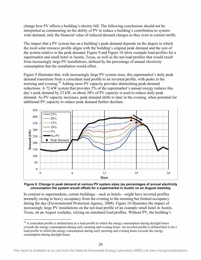
The impact that a PV system has on a building’s peak demand depends on the degree to which the local solar resource profile aligns with the building’s original peak demand and the size of the system relative to the peak demand. Figure 9 and Figure 10 show example load profiles for a supermarket and small hotel in Austin, Texas, as well as the net-load profiles that would result from increasingly large PV installations, defined by the percentage of annual electricity consumption that the installation would offset.

Figure 9 illustrates that, with increasingly large PV system sizes, this supermarket’s daily peak demand transitions from a coincident load profile to an inverted profile, with peaks in the morning and evening.28 Adding more PV capacity provides diminishing peak-demand reductions. A 72-kW system that provides 5% of the supermarket’s annual energy reduces this day’s peak demand by 23 kW, so about 30% of PV capacity is used to reduce daily peak demand. As PV capacity increases, peak demand shifts to later in the evening, when potential for additional PV capacity to reduce peak demand further declines.

Figure 9. Change in peak demand at various PV system sizes (as percentages of annual electricity

consumption the system would offset) for a supermarket in Austin on an August weekday

In contrast to supermarkets, certain buildings—such as hotels—might have inverted profiles normally owing to heavy occupancy from the evening to the morning but limited occupancy during the day (Environmental Protection Agency, 2008). Figure 10 illustrates the impact of increasingly large PV installations on the net-load profile of an example small hotel in Austin, Texas, on an August weekday, relying on simulated load profiles. Without PV, the building’s

28 A coincident profile is defined here as a load profile in which the energy consumption during daylight hours exceeds the energy consumption during early morning and evening hours. An inverted profile is defined here to be a load profile in which the energy consumption during early morning and evening hours exceeds the energy consumption during daylight hours.

0

50

100

150

200

250

300

350

400

450

0 6 12 18 24

Dem

and

(kW

)

Hour

25%20%15%10%5%No PVPeak Demand


peak demand naturally occurs at 8:00 pm, when the potential for PV generation is essentially nonexistent. In this case, no size PV system (at least without some sort of storage or load shifting) could decrease the building’s peak demand. Furthermore, because the on-peak window for this particular utility’s optional TOU demand rates lasts until 8:00 pm, PV could not help capture the potential financial benefits of reducing peak demand in that window.

Figure 10. Change in peak demand at various PV system sizes (as percentages of annual electricity consumption the system would offset) for a small hotel in Austin on an August

weekday

Despite the variation in overall load profiles, once PV was installed, daily peak demand tended to occur in the early evening (around 6:00 pm) for almost every commercial building evaluated. Although this is several hours removed from a typical system peak, this peak remains within the high-TOU window for most utility tariffs.

Figure 11 illustrates how the reductions in each building’s daily peak demand affect the monthly demand charge for that building, as a function of the relative PV system size. For the supermarket, the first 150 kW (9% energy penetration) of installed PV capacity has the greatest impact on demand charges, but additional PV capacity reduces these charges less effectively as the peak demand shifts to a late enough hour that further increases in PV capacity were less effective at decreasing the building’s peak demand. Because PV does not reduce the small hotel’s daily peak demand at any system size, the hotel’s demand charges are unaffected by PV.

0

20

40

60

80

100

120

140

160

0 6 12 18 24

Dem

and

(kW

)

Hour

25%20%15%10%5%No PVPeak Demand


Figure 11. August demand charge as a function of annual energy consumption offset by PV for an

Austin supermarket and small hotel under Austin Energy’s commercial rate for buildings inside the city with a demand greater than 50 kW

The previous three figures consider a PV system’s impact on the daily peak demand of a building. However, the demand charge is typically set by the peak demand over the course of a month, which can limit the ability of PV to reduce such charges owing to the variability of solar resources. Figure 12 illustrates the variation in the TMY3 solar resource profile for a PV module in Hartford, Connecticut, in February, including several days of poor solar resource. This might be less of an issue in the summer, when demand is often highest and solar resource can be consistently strong.

Figure 12. TMY3 solar resource profile for Hartford for the month of February

Figure 13 shows how the variation in solar resource on a particular day would impact the net-load profile of a small office building with a 15-kW PV system. The plot shows the original and net-load profiles for February 13, with a particularly good solar resource, and February 14, with a particularly poor solar resource (per Figure 12). On the good/clear day, PV reduces peak demand moderately. On the poor/overcast day, PV’s impact is very small. Because the month’s demand charge is typically set by the overall peak demand, it likely would be determined by the characteristics of a day with poor solar resource.

These two factors—PV’s limited ability to reduce daily peak demand and the potential for poor solar resource days to determine the month’s peak demand—limit the potential of PV to reduce a particular building’s demand-related charges, as current demand charges are typically calculated.

0123456789

0 0.1 0.2 0.3 0.4 0.5

Mon

thly

Dem

and

Cha

rge

(Tho

usan

ds o

f $)

Fraction of Annual Electricity Consumption Offset by PV)

Supermarket Demand Charge

Small Hotel Demand Charge


Alternative formulations, such as basing a portion of demand charges off of demand during the electric grid system peak, might increase the effect that PV has on demand charges. Solar load controllers and battery systems can increase PV’s impact on a building’s peak demand, as discussed by Herig et al. (2003).

Figure 13. Simulated net-load profile for a small office building in Hartford over 2 days with variable solar resource (one high day, one low day)

4.2 PV Systems Effect on a Building’s Energy Charges In contrast to the limited effects on a building’s peak demand, PV systems offset a building’s energy consumption regardless of load profile shape. For example, a 50-kW system in Minneapolis will generate 62 MWh of energy annually whether it is installed on the roof of a restaurant, hospital, or school. Differences in the value of the generated electricity depend only on the structure of the energy rates for that particular building (i.e., tiered versus TOU).

Figure 14 shows the relative proportion of June’s electricity use and demand charges for four example buildings in four different locations, for various PV system sizes. For example, in the case of the supermarket in Austin, adding a 200-kW PV system would decrease the energy charges by $2,527 but only decrease the demand charges by $869 compared to the same building with no installed PV. Larger PV systems further decrease the energy charges, but effects on demand charges with increasing system size would decline until they were negligible, for the reasons described in Section 4.1.

Although an in-depth analysis of different rate structures across many utilities is beyond the scope of this report, these results suggest that PV systems tend to provide significantly higher economic value by offsetting energy consumption than by decreasing peak demand. This would seem to indicate that when choosing an electricity rate between several offered by a utility, the one with the lower proportion of demand charges would be most financially attractive for a building with PV, but this is not always the case. For instance, many utilities offer rates with no demand component and a very high energy charge. For most of the buildings considered in this study, even with energy generation from the largest-possible PV system, the energy-only option usually is more expensive than the rate with a demand component. Therefore, a building owner that is installing PV should thoroughly evaluate expected bill savings for all eligible rates offered by a utility, rather than relying on the presence or absence of a demand component to indicate which one is financially preferable.


Figure 14. June monthly charges for a supermarket (Austin, commercial inside-city rate), small

hotel (Miami, GSDT-1 rate), full-service restaurant (Seattle, MDD rate), and hospital (Albuquerque, GPS-TOU rate)

0

2

4

6

8

10

12

14

16

0 100 200 300 400

Mon

thly

Cha

rge

(Tho

usan

ds o

f $)

System nameplate capacity (kWDC)

Supermarket in Austin

0

0.5

1

1.5

2

2.5

3

3.5

4

0 50 100 150

Mon

thly

Cha

rge

(Tho

usan

ds o

f $)


Small Hotel in Miami

Demand Charges Volumetric Energy Charges

0

0.5

1

1.5

2

2.5

0 25 50 75 100

Mon

thly

Cha

rge

(Tho

usan

ds o

f $)


Restaurant in Seattle

05

101520253035404550

0 250 500 750 1000

Mon

thly

Cha

rge

(Tho

usan

ds o

f $)


Hospital in Albuquerque


4.3 Breakeven Price Range by Building Type The points above illustrate key considerations affecting the electricity bill savings resulting from PV systems for individual commercial buildings. However, in aggregate, do these and other drivers suggest systematically different breakeven conditions for different building types. Figure 15 presents breakeven values by building type where the distribution reflects results for each utility. As a result, the stated median reflects the median utility result. The median customer breakeven value would likely be higher, owing to the greater concentration of customers in utilities with favorable breakeven conditions, as discussed in Section 4.1.

Figure 15. Nationwide breakeven prices by building type

Owing to the minor reductions in demand charges (see Section 4.1), buildings with coincident load profiles, such as offices, are on average slightly more attractive sites for PV systems than buildings such as hotels, whose peak loads occur outside of the hours when solar resource is available. Overall, however, median breakeven prices across building types vary by less than $0.50/W, because most of the value of a PV system comes from offsetting energy charges. Because a given PV system at a given location generates the same amount of energy regardless of the building it is mounted on, the value of offset energy charges is largely indifferent to building type. The variability among buildings is driven by the minor differences in demand-charge reductions as well as any differences in the cost of energy if different buildings used different rates from the same utility.

On the other hand, variation within building types located in different utility service areas is much greater—$3/W between the 10th and 90th percentiles—which is a function of the diverse rates available for given building parameters nationwide. This suggests that rates available to a given building should be weighted more than the building type. This finding is consistent with the findings in Ong et al. (2012) and Denholm et al. (2009). For example, although small offices have the highest average breakeven price, many small offices might be good candidates and many others poor candidates for PV installation, depending on their local electricity prices and solar resource quality.


5 Conclusion Historically, PV adoption in the commercial sector has faced barriers such as building leasing, lack of awareness by corporate decision makers, and shorter building occupancy. However, recent forecasts and market moves suggest the commercial sector may be poised for growth (GTM Research and SEIA 2015b).

We characterize PV’s economic feasibility in the U.S. commercial sector by modeling 15 different building types in 1,355 utility territories. This analysis suggests that approximately 32% - 64% of commercial customers could break even, depending on the financing mechanism, given today’s costs and 30% ITC. Buildings in some utility areas are on the cusp of breakeven conditions, and additional reductions in installed costs as well as additional revenue from SRECs or state incentives could open many more markets. Our analysis suggests that retail rates are the biggest driver of PV financial attractiveness. Building type differences drive more modest differences.

However, many hurdles to commercial PV remain. In many parts of the country, retail electricity rates remain too low for PV to provide a competitive return at current PV costs. Part of the challenge is that commercial customers often face multi-part rate structures including energy charges, fixed charges, and demand charges, and the potential for PV to reduce demand-related charges as they are currently determined is limited. Future work could include both investigating the potential of energy storage and demand shifting to strengthen PV’s ability to decrease demand charges across a representative set of buildings that captures the diversity of the national stock, as well as investigating alternative formulations of demand charges.

This analysis has several limitations that merit additional refinement. First, it relies on hourly demand and PV-generation data, though many demand intervals are sub-hourly. To better quantify the impact of demand-related limitations on PV economics, further research with sub-hourly load and PV data is merited. Second, this analysis excludes state incentives and SRECs, which in many parts of the country provide an essential source of revenue for commercial PV system owners. Third, given the paramount importance of retail rates (over building type and solar resource), future research could explore factors that impact retail rate savings. For example, future research could evaluate systematically optimizing PV system design to maximize retail rate savings, leveraging research by Rhodes et al. (2014). As debates around net-metering regulations continue to develop, sensitivity of the sector to net-metering regulations will be a critical question. Finally, this analysis only evaluates bill savings, and does not address many additional factors that may present critical incentives or disincentives to businesses considering solar.


References Alliance to Save Energy. 2013. Residential and Commercial Buildings. Washington, DC: Alliance to Save Energy. www.ase.org/sites/ase.org/files/ee_commission_building_report_2-1-13.pdf.

Barnes, Justin, Chad Laurent, Jayson Uppal, Chelsea Barnes, and Amy Heinemann. 2013. Property Taxes and Solar PV Systems: Policies, Practices, and Issues. Raleigh, NC: North Carolina Clean Energy Technology Center. http://nccleantech.ncsu.edu/wp-content/uploads/Property-Taxes-and-Solar-PV-Systems-2013.pdf.

Chung, D., C. Davidson, R. Fu, K. Ardani, and R. Margolis. 2015. U.S. Photovoltaic (PV) Prices and Cost Breakdowns: Q1 2015 Benchmarks for Residential, Commercial, and Utility-Scale Systems. NREL/TP-6A2- 64746. Golden, CO: National Renewable Energy Laboratory.

Darghouth, N., G. Barbose, and R. Wiser. 2013. Electricity Bill Savings from Residential Photovoltaic Systems: Sensitivities to Changes in Future Electricity Market Conditions. LBNL-6017E. Berkeley, CA: Lawrence Berkeley National Laboratory.

Darghouth, N., R. Wiser and G. Barbose,. 2015. Net Metering and Market Feedback Loops: Exploring the Impact of Retail Rate Design on Distributed PV Deployment. LBNL-6017E. Berkeley, CA: Lawrence Berkeley National Laboratory.

Denholm, P., and R.M. Margolis. 2007. “Evaluating the Limits of Solar Photovoltaics (PV) in Traditional Electric Power Systems.” Energy Policy 35: 2852–61.

Denholm, P., R. Margolis, S. Ong, and B. Roberts. 2009. Breakeven Cost for Residential Photovoltaics in the United States: Key Drivers and Sensitivities. NREL/TP-6A2-46909. Golden, CO: National Renewable Energy Laboratory.

Deru, M., K. Field, D. Studer, K. Benne, B. Griffith, and P. Torcellini. 2011. U.S. Department of Energy Commercial Reference Building Models of the National Building Stock. NREL/TP-5500-46861. Golden, CO: National Renewable Energy Laboratory.

DOE (U.S. Department of Energy). 2010. Website: Office of Energy Efficiency and Renewable Energy, Commercial Buildings. http://energy.gov/eere/buildings/about-commercial-buildings-integration-program

DOE (U.S. Department of Energy). 2012. 2011 Buildings Energy Databook. Washington, DC: U.S. Department of Energy.

DSIRE (Database of State Incentives for Renewables & Efficiency). 2015. “Net Metering.” Accessed August 1, 2015. www.dsireusa.org/resources/detailed-summary-maps/net-metering-policies-2/.

EIA (U.S. Energy Information Administration). 2014. Monthly Electric Sales and Revenue Report with State Distributions Report. EIA-826. Washington, DC: U.S. Energy Information Administration.

http://www.ase.org/sites/ase.org/files/ee_commission_building_report_2-1-13.pdf

http://www.ase.org/sites/ase.org/files/ee_commission_building_report_2-1-13.pdf

http://nccleantech.ncsu.edu/wp-content/uploads/Property-Taxes-and-Solar-PV-Systems-2013.pdf

http://nccleantech.ncsu.edu/wp-content/uploads/Property-Taxes-and-Solar-PV-Systems-2013.pdf

http://energy.gov/eere/buildings/about-commercial-buildings-integration-program

http://energy.gov/eere/buildings/about-commercial-buildings-integration-program

http://www.dsireusa.org/resources/detailed-summary-maps/net-metering-policies-2/

http://www.dsireusa.org/resources/detailed-summary-maps/net-metering-policies-2/


EIA (U.S. Energy Information Administration). 2015. Commercial Building Energy Consumption Survey (CBECS). Washington, DC: U.S. Energy Information Administration.

Environmental Protection Agency (2008). Sector Collaborative on Energy Efficiency Accomplishments and Next Steps. Washington, DC: US Environmental Protection Agency.

Feldman, D., and R. Margolis. 2014. To Own or Lease Solar: Understanding Commercial Retailers’ Decisions to Use Alternative Financing Models. NREL/TP-6A20-63216. Golden, CO: National Renewable Energy Laboratory.

Feldman, D., R. Margolis, and D. Boff. 2015. Q1/Q2 2015 Solar Industry Update. Washington, DC: U.S. Department of Energy.

Gilman, P., and A. Dobos. 2012. System Advisor Model, SAM 2011.12.2: General Description. NREL/TP-6A20-53437. Golden, CO: National Renewable Energy Laboratory.

GTM Research and SEIA (Solar Energy Industries Association). 2015a. U.S. Solar Market Insight Report: Q1 2015. Boston: GTM Research and Solar Energy Industries Association.

GTM Research and SEIA (Solar Energy Industries Association). 2015b. U.S. Solar Market Insight 2014 Year-in-Review. Boston: GTM Research and Solar Energy Industries Association.

Herig, C., S. Gouchoe, R. Perez, and T. Hoff. 2003. “PV in Commercial Buildings - Mapping the Breakeven Turn-Key Value of State Markets.” Proceedings of ASES Annual Meeting, Austin, Texas.

Gagnon, P., R. Margolis, J. Melius, C. Phillips, and R. Elmore. (forthcoming) Rooftop Photovoltaic Technical Potential in the United States: A Detailed Assessment. NREL Technical Report. NREL/TP-6A20-XXXXX. Golden, CO: National Renewable Energy Laboratory.

NCSL (National Conference of State Legislators). 2015. “Net Metering: Policy Overview and State Legislative Updates.” Accessed August 2, 2015. www.ncsl.org/research/energy/net-metering-policy-overview-and-state-legislative-updates.aspx.

Ong, S., C. Campbell, and N. Clark. 2012. Impacts of Regional Electricity Prices and Building Type on the Economics of Commercial Photovoltaic Systems. NREL/TP-6A20-56461. Golden, CO: National Renewable Energy Laboratory.

Ong, S., N. Clark, P. Denholm, and R. Margolis. 2013. Breakeven Prices for Photovoltaics on Supermarkets in the United States. NREL/TP-6A20-57276. Golden, CO: National Renewable Energy Laboratory.

Ong,S., P. Denholm. 2011. Maximizing the Value of Photovolotaic Installations on Schools in California: Choosing the Best Electricity Rates. NREL/TP-6A20-51694. Golden, CO: National Renewable Energy Laboratory.

http://www.nrel.gov/docs/fy15osti/63216.pdf

http://www.nrel.gov/docs/fy15osti/63216.pdf

http://www.ncsl.org/research/energy/net-metering-policy-overview-and-state-legislative-updates.aspx

http://www.ncsl.org/research/energy/net-metering-policy-overview-and-state-legislative-updates.aspx


Ong, S., P. Denholm, and E. Doris. 2010. The Impacts of Commercial Electric Utility Rate Structure Elements on the Economics of Photovoltaic Systems. NREL/TP-6A2-46782. Golden, CO: National Renewable Energy Laboratory.

Rhodes, J.D., C.R. Upshaw, W.J. Cole, C.L. Holcomb, and M.E. Webber. 2014. “A Multi-Objective Assessment of the Effect of Solar PV Array Orientation and Tilt on Energy Production and System Economics.” Solar Energy 108: 28–40.

Sol Systems. 2015. Sol Systems Project Finance Journal, April 2015. Washington, DC: Sol Systems.

Wilcox, S., and W. Marion. 2008. Users Manual for TMY3 Data Sets. NREL/TP-581-43156. Golden, CO: National Renewable Energy Laboratory.

Wiser, R., A. Mills, G. Barbose, and W. Golove. 2007. The Impact of Retail Rate Structures on the Economics of Commercial Photovoltaic Systems in California. LBNL-63019. Berkeley, CA: Lawrence Berkeley National Laboratory.

http://www.sciencedirect.com/science/article/pii/S0038092X14003314



Documents

Nationwide Analysis of U.S. Commercial Building Solar Photovoltaic