arX

iv:1

309.

1602

v2 [

stat

.AP]

19

Jan

2015

The Annals of Applied Statistics

2014, Vol. 8, No. 4, 2122–2149DOI: 10.1214/14-AOAS768c© Institute of Mathematical Statistics, 2014

GLOBAL ESTIMATION OF CHILD MORTALITY USINGA BAYESIAN B-SPLINE BIAS-REDUCTION MODEL1

By Leontine Alkema and Jin Rou New

National University of Singapore

Estimates of the under-five mortality rate (U5MR) are used totrack progress in reducing child mortality and to evaluate countries’performance related to Millennium Development Goal 4. However, forthe great majority of developing countries without well-functioningvital registration systems, estimating the U5MR is challenging dueto limited data availability and data quality issues.

We describe a Bayesian penalized B-spline regression model for as-sessing levels and trends in the U5MR for all countries in the world,whereby biases in data series are estimated through the inclusion of amultilevel model to improve upon the limitations of current methods.B-spline smoothing parameters are also estimated through a multi-level model. Improved spline extrapolations are obtained through log-arithmic pooling of the posterior predictive distribution of country-specific changes in spline coefficients with observed changes on theglobal level.

The proposed model is able to flexibly capture changes in U5MRover time, gives point estimates and credible intervals reflecting po-tential biases in data series and performs reasonably well in out-of-sample validation exercises. It has been accepted by the United Na-tions Inter-agency Group for Child Mortality Estimation to generateestimates for all member countries.

1. Introduction. The under-five mortality rate (U5MR) is a key barom-eter of the well-being of a country’s children and, more broadly, an indicatorof socioeconomic progress. The U5MR is strictly not a rate, but the prob-ability that a child born in a given year will die before reaching the age offive if subject to current age-specific mortality rates (UN IGME 2013), often

Received May 2014.1Supported by Grants R-155-000-099-133 and R-155-000-146-112 at the National Uni-

versity of Singapore and the United Nations Children’s Fund.Key words and phrases. Bayesian hierarchical model, Millennium Development Goal 4,

logarithmic pooling, penalized B-spline regression model, under-five mortality rate, UnitedNations Inter-agency Group for Child Mortality Estimation.

This is an electronic reprint of the original article published by theInstitute of Mathematical Statistics in The Annals of Applied Statistics,2014, Vol. 8, No. 4, 2122–2149. This reprint differs from the original in paginationand typographic detail.

1

2 L. ALKEMA AND J. R. NEW

expressed as the number of deaths per 1000 live births. National estimatesof the U5MR are used to track progress in reducing child mortality and toevaluate countries’ performance with respect to the United Nations’ Millen-nium Development Goal 4 (MDG 4), which calls for a two-thirds reductionin the U5MR between 1990 and 2015 (UN IGME 2013), corresponding toan annual rate of reduction of 4.4%.

For the great majority of developing countries without well-functioningvital registration systems, estimating levels and trends in U5MR is chal-lenging, not only because of limited data availability but also because ofissues with data quality. Every year, the United Nations Inter-agency Groupfor Child Mortality Estimation (UN IGME, including the United NationsChildren’s Fund, the World Health Organization, the World Bank, and theUnited Nations Population Division) produces and publishes estimates ofchild mortality comparable across countries and years for 194 countries. In2012, a Loess regression model was used to estimate the U5MR (UN IGME2012). For each country, the default setting for its smoothness parameter αwas determined by the type and availability of data in the country. A boot-strap method was used to assess the uncertainty in the U5MR estimates[Alkema and New (2012)]. A number of limitations with this approach wereidentified. The first limitation was that for a subset of countries, the fittedLoess curve was deemed to not fit the data well and post-hoc adjustments inthe α value were necessary. The second limitation was that all observationswere weighted equally to obtain point estimates; standard errors, potentialdata biases and indicators of data quality were not accounted for. The cali-bration of the resulting point estimates and uncertainty intervals left roomfor improvement.

Alternative methods for estimating child mortality for all countries havebeen developed by the Institute for Health Metrics and Evaluation (IHME)[Rajaratnam et al. (2010), Wang et al. (2012)], which uses Gaussian processregression modeling to obtain U5MR estimates. A model validation exer-cise to check model performance based on the 2010 version of the IHMEapproach also indicated room for improvement [Alkema, Wong and Seah(2012)], possibly explained by the approach not fully accounting for poten-tial data biases. To the best of our knowledge, the same exercise has notbeen repeated for the most recent iteration of the IHME model [Wang et al.(2012)]. We expect that issues with model calibration have not yet been fullyaddressed given that the data model has not been updated to incorporatethe possibility of data biases.

In this paper we propose an alternative U5MR estimation approach toimprove upon the limitations and lack of calibration of existing methods.The approach is given by a Bayesian B-spline Bias-reduction model, referredto as the B3 model. The UN IGME has decided to use the B3 model toassess countries’ progress toward MDG 4 and B3 estimates are included

GLOBAL ESTIMATION OF CHILD MORTALITY 3

in “A Promise Renewed Progress Report 2013” [United Nations Children’sFund, Division of Policy and Strategy (2013)] and the “Child MortalityReport 2013” (UN IGME 2013).

The paper is organized as follows. Section 2 provides background infor-mation on child mortality estimation. In Section 3 we present the B3 modelspecification, followed by validation results and resulting U5MR estimatesin Section 4. We end with a discussion of the model and scope for futureresearch.

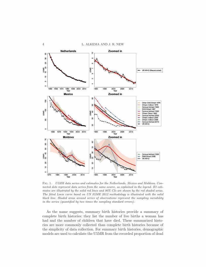
2. Background. U5MR data series are constructed from information fromvital registration (VR) and sample vital registration (SVR) systems, surveysand censuses. U5MR data for selected countries are shown in Figures 1 and 2.The selected countries differ with respect to U5MR level and trend, as wellas data availability and data quality.

In the Netherlands, data from the VR system capturing all births anddeaths are available since 1940. Such data from well-functioning VR sys-tems are the preferred data source for calculating U5MR. However, in 2013,60 countries for which the UN IGME produces U5MR estimates did nothave any data from VR systems. Among the 135 countries with VR or SVRsystems, recording of birth and/or deaths is not necessarily complete; illus-trations are given for Mexico and Moldova. In Mexico, VR data were deemedcomplete only since 2005. For Moldova, VR data are considered incompletefor all observation years.

For countries without (or with limited information from) well-functioningVR systems, complete or summary birth histories of women, collected insurveys and censuses, are often the main source of information on U5MR.A complete birth history lists all the live births a woman has had, includinginformation on the date of birth of each child, whether the child is still alive,and if the child has died, the age at death. U5MR observations are calcu-lated from such information through a synthetic cohort approach, wherebyfor a given period before the survey, survival probabilities are calculated forsmall age intervals and combined to obtain the U5MR for that period [Ped-ersen and Liu (2012)]. These observations are referred to as direct estimatesof U5MR. Many of these direct series are obtained from complete birthhistories that were collected as part of the international household surveyprogram Demographic and Health Surveys (DHS). Other direct series areobtained from data from survey programs similar to the DHS [here referredto as Other DHS as opposed to (Standard) DHS], as well as other nationalsurveys (referred to as Others Direct). Examples of direct series are shownin Figures 1 and 2. Because of the retrospective nature of the data, directseries can extend for up to decades before the survey. For example, the DHSin Cambodia that was carried out in 2005–2006 provides data from 1979 to2004.

4 L. ALKEMA AND J. R. NEW

Fig. 1. U5MR data series and estimates for the Netherlands, Mexico and Moldova. Con-nected dots represent data series from the same source, as explained in the legend. B3 esti-mates are illustrated by the solid red lines and 90% CIs are shown by the red shaded areas.The fitted Loess curve based on UN IGME 2012 methodology is illustrated with the solidblack line. Shaded areas around series of observations represent the sampling variabilityin the series (quantified by two times the sampling standard errors).

As the name suggests, summary birth histories provide a summary ofcomplete birth histories: they list the number of live births a woman hashad and the number of children that have died. These summarized histo-ries are more commonly collected than complete birth histories because ofthe simplicity of data collection. For summary birth histories, demographicmodels are used to calculate the U5MR from the recorded proportion of dead

GLOBAL ESTIMATION OF CHILD MORTALITY 5

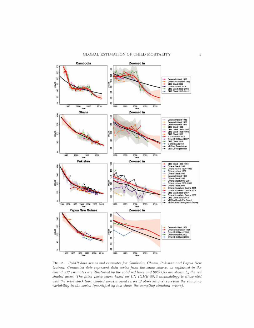
Fig. 2. U5MR data series and estimates for Cambodia, Ghana, Pakistan and Papua NewGuinea. Connected dots represent data series from the same source, as explained in thelegend. B3 estimates are illustrated by the solid red lines and 90% CIs are shown by the redshaded areas. The fitted Loess curve based on UN IGME 2012 methodology is illustratedwith the solid black line. Shaded areas around series of observations represent the samplingvariability in the series (quantified by two times the sampling standard errors).

6 L. ALKEMA AND J. R. NEW

children for different time references [Brass (1964), United Nations (1983)].Because of the dependency on models, these estimates based on summarybirth histories are referred to as indirect estimates. Indirect series are mostcommonly obtained using information from censuses and surveys such asthe Multiple Indicator Cluster Survey (MICS), an international survey pro-gram that collects summary birth histories in many developing countries.Examples of indirect series are shown in Figures 1 and 2. As discussed fordirect data series, indirect series also provide data points for a long ret-rospective period. For example, the Cambodian census from 1998 providesindirect estimates from 1983 to 1994.

The availability of nationally-representative surveys and censuses carriedout in developing countries varies greatly. For instance, a large number ofdata series are available from various sources in Pakistan, but only five dataseries are available for Papua New Guinea. Moreover, data series do notnecessarily tell a similar story about levels and/or trends in U5MR. Forexample, in Papua New Guinea, there are large differences between U5MRestimates from the various sources. In Pakistan, the DHS 2006–2007 surveysuggests lower levels of U5MR than data from its sample registration system.The spread in data points for countries without data from well-functioningVR systems is not specific to the selected countries in Figures 1 and 2, but isobserved in many developing countries, as U5MR data are associated witha variety of data quality issues. Apart from sampling error, observationsfrom non-VR sources may also be subject to bias and nonsampling error,for example, because of recall biases when collecting birth histories. Specificdata series may be entirely biased upward or downward, for example, basedon inaccuracies in the indirect estimation method that was used to translatethe summary birth histories from a census or survey in U5MR observations.

Given issues with data quantity and quality, estimating the U5MR ischallenging for many countries. A modeling approach needs to be flexibleenough to capture short-term fluctuations in U5MR without being overlysensitive to erroneous data fluctuations.

3. Constructing U5MR estimates. We developed a modeling approachthat combines a flexible curve fitting method with a comprehensive datamodel to account for data quality issues. In the model description, lowercaseGreek letters refer to unknown parameters, uppercase Greek letters to func-tions of unknown parameters, and Roman letters to fixed variables, includingdata (lowercase). Λc(t) denotes the quantity of interest, the true U5MR incountry c in year t. U5MR observations are combined across countries andindexed by i = 1,2, . . . ,N ; ui denotes observed U5MR for observation i incountry c[i] and year t[i].

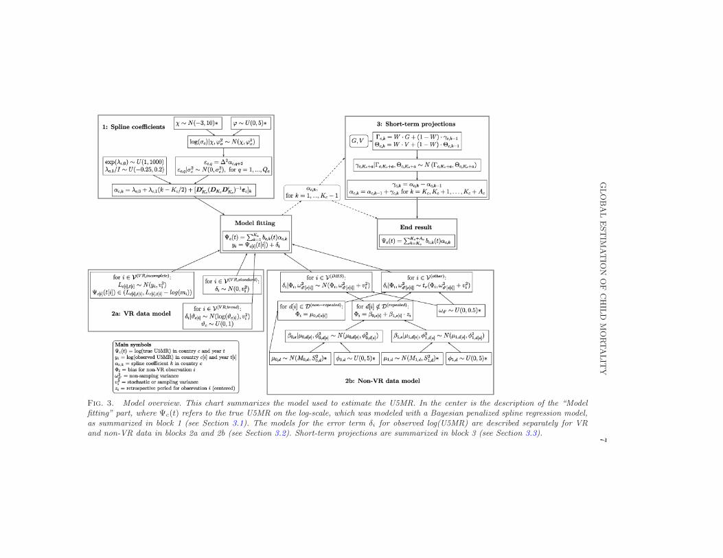
The complete model overview is given in Figure 3. In the center of theoverview and the model is the description of the “Model fitting” for the

GLOBALESTIM

ATIO

NOF

CHIL

DMORTALIT

Y7

Fig. 3. Model overview. This chart summarizes the model used to estimate the U5MR. In the center is the description of the “Modelfitting” part, where Ψc(t) refers to the true U5MR on the log-scale, which was modeled with a Bayesian penalized spline regression model,as summarized in block 1 (see Section 3.1). The models for the error term δi for observed log(U5MR) are described separately for VRand non-VR data in blocks 2a and 2b (see Section 3.2). Short-term projections are summarized in block 3 (see Section 3.3).

8 L. ALKEMA AND J. R. NEW

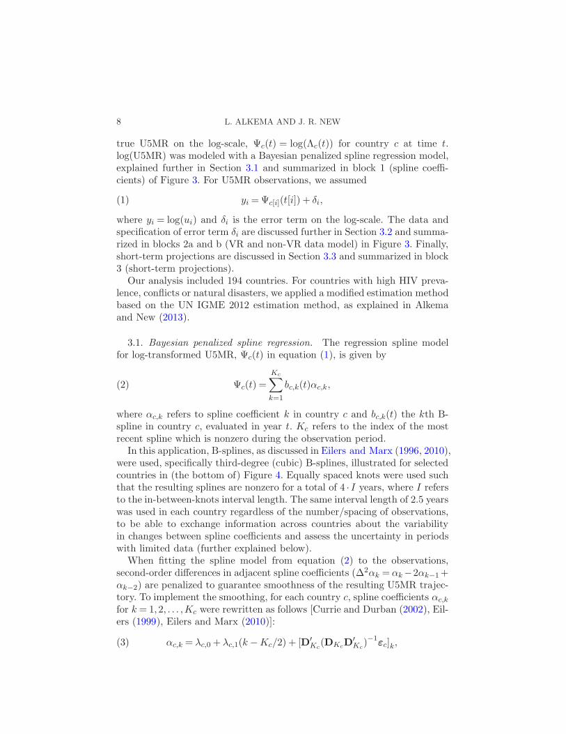
true U5MR on the log-scale, Ψc(t) = log(Λc(t)) for country c at time t.log(U5MR) was modeled with a Bayesian penalized spline regression model,explained further in Section 3.1 and summarized in block 1 (spline coeffi-cients) of Figure 3. For U5MR observations, we assumed

yi =Ψc[i](t[i]) + δi,(1)

where yi = log(ui) and δi is the error term on the log-scale. The data andspecification of error term δi are discussed further in Section 3.2 and summa-rized in blocks 2a and b (VR and non-VR data model) in Figure 3. Finally,short-term projections are discussed in Section 3.3 and summarized in block3 (short-term projections).

Our analysis included 194 countries. For countries with high HIV preva-lence, conflicts or natural disasters, we applied a modified estimation methodbased on the UN IGME 2012 estimation method, as explained in Alkemaand New (2013).

3.1. Bayesian penalized spline regression. The regression spline modelfor log-transformed U5MR, Ψc(t) in equation (1), is given by

Ψc(t) =

Kc∑

k=1

bc,k(t)αc,k,(2)

where αc,k refers to spline coefficient k in country c and bc,k(t) the kth B-spline in country c, evaluated in year t. Kc refers to the index of the mostrecent spline which is nonzero during the observation period.

In this application, B-splines, as discussed in Eilers and Marx (1996, 2010),were used, specifically third-degree (cubic) B-splines, illustrated for selectedcountries in (the bottom of) Figure 4. Equally spaced knots were used suchthat the resulting splines are nonzero for a total of 4 · I years, where I refersto the in-between-knots interval length. The same interval length of 2.5 yearswas used in each country regardless of the number/spacing of observations,to be able to exchange information across countries about the variabilityin changes between spline coefficients and assess the uncertainty in periodswith limited data (further explained below).

When fitting the spline model from equation (2) to the observations,second-order differences in adjacent spline coefficients (∆2αk = αk−2αk−1+αk−2) are penalized to guarantee smoothness of the resulting U5MR trajec-tory. To implement the smoothing, for each country c, spline coefficients αc,k

for k = 1,2, . . . ,Kc were rewritten as follows [Currie and Durban (2002), Eil-ers (1999), Eilers and Marx (2010)]:

αc,k = λc,0 + λc,1(k−Kc/2) + [D′

Kc(DKc

D′

Kc)−1

εc]k,(3)

GLOBAL ESTIMATION OF CHILD MORTALITY 9

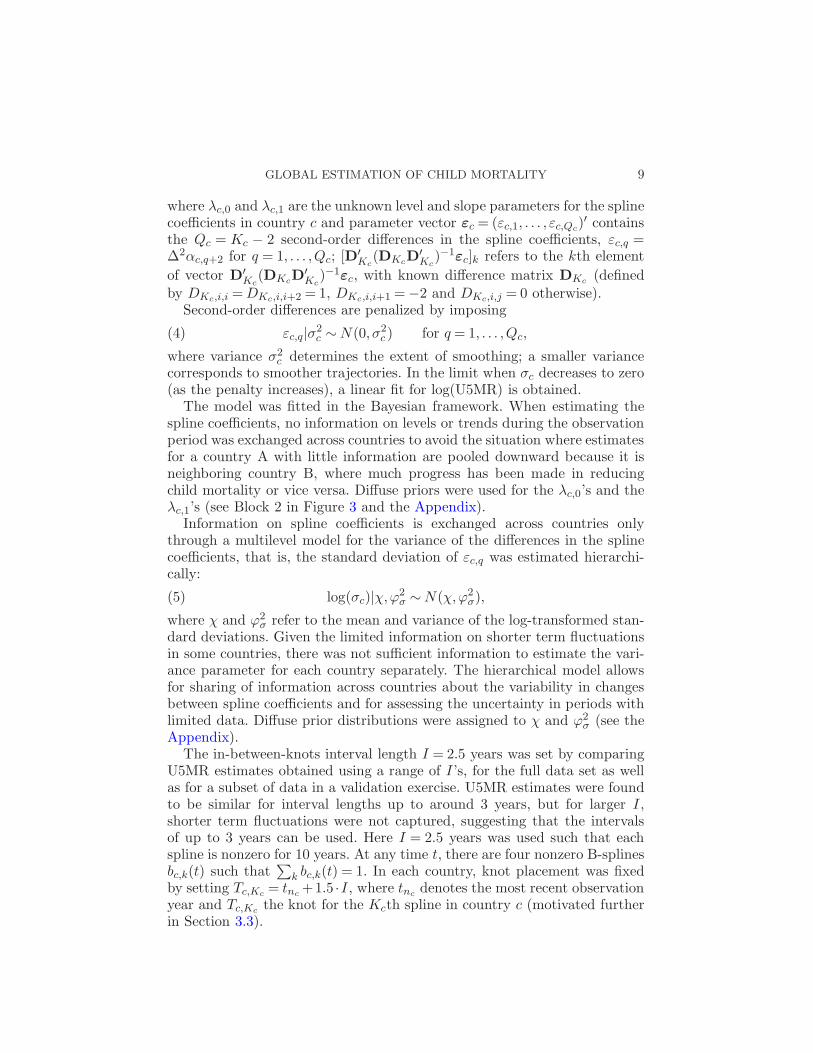
where λc,0 and λc,1 are the unknown level and slope parameters for the splinecoefficients in country c and parameter vector εc = (εc,1, . . . , εc,Qc

)′ containsthe Qc = Kc − 2 second-order differences in the spline coefficients, εc,q =∆2αc,q+2 for q = 1, . . . ,Qc; [D

′

Kc(DKc

D′

Kc)−1

εc]k refers to the kth element

of vector D′

Kc(DKc

D′

Kc)−1

εc, with known difference matrix DKc(defined

by DKc,i,i =DKc,i,i+2 = 1, DKc,i,i+1 =−2 and DKc,i,j = 0 otherwise).Second-order differences are penalized by imposing

εc,q|σ2c ∼N(0, σ2

c ) for q = 1, . . . ,Qc,(4)

where variance σ2c determines the extent of smoothing; a smaller variance

corresponds to smoother trajectories. In the limit when σc decreases to zero(as the penalty increases), a linear fit for log(U5MR) is obtained.

The model was fitted in the Bayesian framework. When estimating thespline coefficients, no information on levels or trends during the observationperiod was exchanged across countries to avoid the situation where estimatesfor a country A with little information are pooled downward because it isneighboring country B, where much progress has been made in reducingchild mortality or vice versa. Diffuse priors were used for the λc,0’s and theλc,1’s (see Block 2 in Figure 3 and the Appendix).

Information on spline coefficients is exchanged across countries onlythrough a multilevel model for the variance of the differences in the splinecoefficients, that is, the standard deviation of εc,q was estimated hierarchi-cally:

log(σc)|χ,ϕ2σ ∼N(χ,ϕ2

σ),(5)

where χ and ϕ2σ refer to the mean and variance of the log-transformed stan-

dard deviations. Given the limited information on shorter term fluctuationsin some countries, there was not sufficient information to estimate the vari-ance parameter for each country separately. The hierarchical model allowsfor sharing of information across countries about the variability in changesbetween spline coefficients and for assessing the uncertainty in periods withlimited data. Diffuse prior distributions were assigned to χ and ϕ2

σ (see theAppendix).

The in-between-knots interval length I = 2.5 years was set by comparingU5MR estimates obtained using a range of I ’s, for the full data set as wellas for a subset of data in a validation exercise. U5MR estimates were foundto be similar for interval lengths up to around 3 years, but for larger I ,shorter term fluctuations were not captured, suggesting that the intervalsof up to 3 years can be used. Here I = 2.5 years was used such that eachspline is nonzero for 10 years. At any time t, there are four nonzero B-splinesbc,k(t) such that

∑k bc,k(t) = 1. In each country, knot placement was fixed

by setting Tc,Kc= tnc

+1.5 ·I , where tncdenotes the most recent observation

year and Tc,Kcthe knot for the Kcth spline in country c (motivated further

in Section 3.3).

10 L. ALKEMA AND J. R. NEW

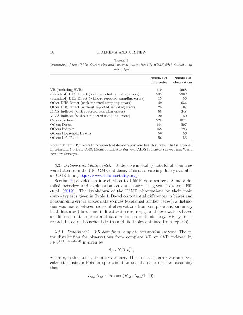
Table 1

Summary of the U5MR data series and observations in the UN IGME 2013 database bysource type

Number of Number ofdata series observations

VR (including SVR) 110 2968(Standard) DHS Direct (with reported sampling errors) 203 2902(Standard) DHS Direct (without reported sampling errors) 15 56Other DHS Direct (with reported sampling errors) 49 634Other DHS Direct (without reported sampling errors) 25 107MICS Indirect (with reported sampling errors) 55 248MICS Indirect (without reported sampling errors) 20 80Census Indirect 228 1074Others Direct 144 507Others Indirect 168 793Others Household Deaths 56 56Others Life Table 56 56

Note: “Other DHS” refers to nonstandard demographic and health surveys, that is, Special,Interim and National DHS, Malaria Indicator Surveys, AIDS Indicator Surveys and WorldFertility Surveys.

3.2. Database and data model. Under-five mortality data for all countrieswere taken from the UN IGME database. This database is publicly availableon CME Info (http://www.childmortality.org).

Section 2 provided an introduction to U5MR data sources. A more de-tailed overview and explanation on data sources is given elsewhere [Hillet al. (2012)]. The breakdown of the U5MR observations by their mainsource types is given in Table 1. Based on potential differences in biases andnonsampling errors across data sources (explained further below), a distinc-tion was made between series of observations from complete and summarybirth histories (direct and indirect estimates, resp.), and observations basedon different data sources and data collection methods (e.g., VR systems,records based on household deaths and life tables obtained from reports).

3.2.1. Data model. VR data from complete registration systems. The er-ror distribution for observations from complete VR or SVR indexed byi ∈ V(VR standard) is given by

δi ∼N(0, v2i ),

where vi is the stochastic error variance. The stochastic error variance wascalculated using a Poisson approximation and the delta method, assumingthat

Dc,t|Λc,t ∼ Poisson(Bc,t ·Λc,t/1000),

GLOBAL ESTIMATION OF CHILD MORTALITY 11

where Dc,t is the number of under-five deaths and Bc,t is the number of livebirths for country c in year t.

The number of births were obtained from the World Population Prospects[United Nations, Department of Economic and Social Affairs, PopulationDivision (2011)] and stochastic errors were set to a minimum of 0.025 (i.e.,2.5%). For VR-type data from sample vital registration systems where thenumber of sampled live births was not available, it was set to 0.1 (i.e., 10%)based on the target standard error for the Indian sample registration system(Census of India, 2011).

VR observations were typically calculated for single-year periods butlonger periods were used for smaller countries in instances where the co-efficient of variation of the observation was larger than 10% (due to smallnumbers of births and deaths).

VR data from incomplete registration systems. For 10 countries in theregional grouping of the Central and Eastern Europe/Commonwealth of In-dependent States (CEE/CIS) (namely, Armenia, Azerbaijan, Georgia, Kaza-khstan, Kyrgyzstan, Moldova, Tajikistan, Turkmenistan, Ukraine and Uzbek-istan), VR data were incomplete with respect to the reporting of deaths(biased downward) and generally excluded from the estimation procedurein previous rounds of UN IGME estimation. However, although not infor-mative about the level of U5MR, these observations were deemed to provideinformation on U5MR in the early 1990s and for recent years. During theearly 1990s, in several CEE/CIS countries, data from the VR suggested aplateauing of or even an increase in U5MR. This is illustrated in Figure 1for Moldova. This observed trend is assumed to reflect a true stagnation inprogress in reducing U5MR. To use this information, we incorporated theoption to include incomplete VR data into the model to inform trend esti-mates in the country-specific B3 model. We also included the option to setupper and lower bounds for recent years. (These options were used in thecountry-specific models, as described in Section 3.5.)

To use the observed trend in VR data in the early 1990s to inform theU5MR estimates, the VR observation in 1990 and the maximum observedVR observation from 1991 to 1995 in each CEE/CIS country were selected,with indices denoted by index set V (VR,trend). For each selected observationi ∈ V (VR,trend), the distribution of the error term δi was given by

δi|ϑc[i] ∼N(log(ϑc[i]), v2i ),

ϑc ∼ U(0,1),

where country-specific bias parameter ϑc[i] was added such that the twoselected observations in country c could inform the trend in U5MR estimatesbut not the level.

For the most recent period starting from 2005, for a subset of CEE/CIScountries, U5MR extrapolations based on the global model either decreased

12 L. ALKEMA AND J. R. NEW

below incomplete VR observations (where incomplete refers to incompletereporting of deaths resulting in downward biased VR observations) or theextrapolation resulted in estimates far above VR observations for which anexternal assessment of VR data by the UN IGME suggested a minimumlevel of completeness ranging from 50% to 90%. We resolved the U5MRdiscrepancies between the B3 extrapolations and (assumed completenessof) VR data by including a subset of VR observations as a minimum U5MRvalue into the model (accounting for stochastic errors). More precisely, basedon the most recent incomplete VR observation yi (with i ∈ V(VR,incomplete)),the lower bound Lc[i],t[i] for the log(U5MR) for country c[i] in year t[i] wasobtained as follows:

Lc[i],t[i] ∼N(yi, v2i ).

For selected observations, where a minimum level of completeness mi wasset for incomplete VR observation yi, we also included the upper boundLc[i],t[i] − log(mi) for log(U5MR). For example, if the minimum complete-ness for observation i is 80%, then mi = 0.8 and the upper bound for theU5MR is given by exp(Lc[i],t[i])/mi = exp(Lc[i],t[i])/0.8. VR-based upper andlower bounds were incorporated into the model by excluding any log(U5MR)estimates which fell outside the interval (Lc,t,Uc,t).

Non-VR data. For non-VR data, the data model needs to account for (i)sampling and nonsampling errors, (ii) potential biases in trends and levelsof U5MR data series, and (iii) possibility of outliers.

For observations from Standard and Other DHS Direct series, indexed byi ∈ V(DHS), the error was assumed to be normally distributed

δi|Φi,Ω2i ∼N(Φi,Ω

2i ),

with mean bias Φi and standard deviation Ωi. For observations from othersource types, indexed by i ∈ V(other), posterior predictive checks suggestedthat more outliers were present, therefore, a t-distribution with unknown νdegrees of freedoms was used:

δi|Φi,Ω2i ∼ tν(Φi,Ω

2i ),

ν ∼ U(2,30),

where tν(Φi,Ω2i ) denoted a t-distribution with ν degrees of freedom, centered

at Φi and rescaled by Ωi.For observations from non-VR source types d with potentially multiple

observations per series, mean biases were modeled as a linear function of theretrospective period of the observation in the survey (the difference betweenthe observation reference date and the date of the survey/census). Thissetup was motivated by known problems with retrospective data, such asthe occurrence of recall biases and violations of modeling assumptions when

GLOBAL ESTIMATION OF CHILD MORTALITY 13

calculating indirect U5MR observations. The linear model for mean bias Φi

for observation i is given by

Φi = β0,s[i] + β1,s[i] · zi,

where β0,s[i] + β1,s[i] · zi represents the bias in level and trend as a functionof the retrospective period zi for observation i (centered at 10 years) indata series s[i]. The bias in the level of the series β0,s was estimated with amultilevel model:

β0,s|µ0,d[s], φ20,d[s] ∼N(µ0,d[s], φ

20,d[s]),

where d[s] refers to the source type of series s. The set of source types withpotentially multiple observations per series, indexed by D(repeated), is givenby (Standard) DHS Direct, Other DHS Direct (including Special, Interimand National DHS, Malaria Indicator Surveys, AIDS Indicator Surveys andWorld Fertility Surveys), MICS Indirect, Census Indirect, Others Directand Others Indirect. µ0,d and φ2

0,d represent source type-specific mean biasand between-series variance, respectively. These two hyperparameters wereunknown and were assigned prior distributions, as illustrated in Figure 3.

A similar approach was used to estimate the slope β1,s:

β1,s|µ1,d[s], φ21,d[s] ∼N(µ1,d[s], φ

21,d[s]),

where µ1,d and φ21,d represent the mean slope and the between-series variance

for source type d. For observations constructed from source types withoutrepeated observations (reported household deaths and reported life tables,d ∈D(nonrepeated)), we assumed that Φi = µ0,d[s[i]].

Scale parameter Ωi was modeled as a combination of sampling variancev2i and nonsampling variance ω2

d′[s[i]]:

Ω2i = ω2

d′[s[i]]+ v2i ,

where source type d′[s] for series s refers to a further breakdown of sourcetypes to distinguish between DHS, Other DHS and MICS surveys with andwithout reported sampling errors for their observations (as indicated in Ta-ble 1). If the sampling standard errors were not reported, a sampling stan-dard error of 2.5% was used for Census Indirect observations and 10% forall other observations. Nonsampling variance refers to variability because ofrandom errors that arise through imperfections in the data collection processand is unknown.

Hyperparameters µ0,d, φ20,d, µ1,d, φ

21,d, ω

2d′ and ν were assigned prior dis-

tributions, as listed in the Appendix. Diffuse priors were used for all hyper-parameters, with the exception of the mean bias µ0,d for the DHS Directseries: an informative prior distribution was used, based on an analysis ofthese biases in the previous 2012 round of UN IGME estimates.

14 L. ALKEMA AND J. R. NEW

3.3. Extrapolation using a logarithmic pooling approach. The one-step-ahead projection of a future change in spline coefficients based on the pe-nalized spline regression model is given by

γc,k|γc,k−1, σ2c ∼N(γc,k−1, σ

2c ),(6)

where γc,k =∆αc,k = αc,k − αc,k−1. This extrapolation can result in a highprobability of unusually low or high projected rates of change in the splinecoefficients for a specific U5MR trajectory if σc is large and/or if γc,k−1 isunusually small or large. If projected changes in spline coefficients are un-usually low or high over longer periods, so are the projected changes in theU5MR, potentially giving rise to unrealistic U5MR projections. To overcomethis potential problem with the spline extrapolations, we implemented a log-arithmic pooling procedure to combine country-specific posterior predictivedistributions (PPDs) for changes in spline coefficients with a global PPD andverified whether this approach improved out-of-sample projections. This pro-cedure was applied to modify the PPDs for αc,k for k =Kc,Kc + 1, . . . , Pc,where Kc and Pc refer to the indices of the most recent splines in the ob-servation and projection periods, respectively. Spline coefficient αc,Kc

wasincluded in the set of “projected” coefficients to be pooled because it is basedon very limited information only; the Kcth spline is placed such that it isnonzero only for 1.25 years during the observation period, from tnc

− 1.25to tnc

.The approach is summarized as follows (see also block 3 in Figure 3): Let

α(j)c,k denote the jth posterior sample of spline coefficient k for country c, j =

1, . . . , J and let Γ(j)c,k+1 =∆α

(j)c,k+1 = α

(j)c,k+1−α

(j)c,k, the jth posterior sample of

the differences between two adjacent spline coefficients. After fitting the B3

model, we obtain γ(j)c,k for k = 1,2, . . . ,Kc − 1, while γc,k’s for k =Kc,Kc +

1, . . . , Pc are drawn from a pooled PPD (see Figure 4). The pooled PPD is a

combination of the “model-induced” country-specific PPD for γ(j)c,k , defined

by the penalized splines model and a global PPD for future changes in thespline coefficients. The global PPD was based on the set of posterior median

estimates of the γ(j)c,k ’s, γc,k for c = 1, . . . ,C and k = 2, . . . ,Kc − 1 (during

the observation period for each country). We used country-projection-step-specific logarithmic pooling weights to obtain the same extent of pooling for

all countries. The resulting pooled PPD for γ(j)c,Kc+a for a≥ 0 is given by

γ(j)c,Kc+a|Γ

(j)c,Kc+a,Θ

(j)c,Kc+a ∼N(Γ

(j)c,Kc+a,Θ

(j)c,Kc+a),

where

Γ(j)c,k =W ·G+ (1−W ) · γ

(j)c,k−1,

Θ(j)c,k =W · V + (1−W ) ·Θ

(j)c,k−1,

GLOBAL ESTIMATION OF CHILD MORTALITY 15

with G and V equal to the median and variance of the γc,k’s, respectively,

γ(j)c,Kc−1 = α

(j)c,Kc−1 −α

(j)c,Kc−2 and Θ

(j)c,Kc−1 = σ

(j)c .

The overall pooling weight 0 ≤ W ≤ 1 was chosen through an out-of-sample validation exercise (described in Section 3.6). Further details of thelogarithmic pooling procedure are given in the Appendix.

3.4. Computation. A Markov Chain Monte Carlo (MCMC) algorithmwas employed to sample from the posterior distribution of the parameterswith the use of the software JAGS [Plummer (2003)]. Six parallel chains withdifferent starting points were run with a total of 50,000 iterations in eachchain. Of these, the first 10,000 iterations in each chain were discarded asburn-in and every 20th iteration after was retained. The resulting chainscontained 2000 samples each. Standard diagnostic checks (using trace plots,the Raftery and Lewis diagnostic [Raftery and Lewis (1992, 1996)] and theGelman and Rubin diagnostic [Gelman and Rubin (1992)]) were used tocheck convergence.

Estimates of relevant quantities are given by the posterior medians, while90% credible intervals (CIs) were constructed from the 5% and 95% per-centiles of the posterior sample. Given the inherent uncertainty in U5MRestimates, 90% CIs are used by UN IGME instead of the more conventional95% ones.

3.5. Country-specific UN IGME model and adjustments. The B3 modelwas accepted by UN IGME to evaluate countries’ progress and performancein reducing U5MR. For this purpose, a computationally cheaper and moreuser-friendly country-specific model was implemented, with noncountry-specific parameters (marked with a star in Figure 3) fixed at the poste-rior medians from the global model run, which resulted in very similar esti-mates. For the country-specific runs, we ran 6 chains with a total of 35,000iterations in each chain. Of these, the first 10,000 iterations in each chainwere discarded as burn-in and every 20th iteration after was retained. Theresulting chains contained 1250 samples each.

After reviewing the estimates, two model adjustments were incorporatedin the country-specific models to consistently adjust the level of under- orover-smoothing in a subset of countries [see Alkema and New (2013) fordetails].

Adjustments were also applied to the Democratic Republic of Congo andSomalia, where the U5MR data are not deemed to be representative of thecountry’s past. Specifically, B-splines corresponding to conflict periods wherethe U5MR is unlikely to have declined were combined such that only onespline coefficient was estimated for each conflict period. The resulting fit isconstant during the conflict periods.

16 L. ALKEMA AND J. R. NEW

3.6. Model validation. Model performance was assessed through an out-of-sample validation exercise. Given the retrospective nature of U5MR dataand the occurrence of data in series, the training set was not constructed byleaving out observations at random, but based on all available data in someyear in the past [Alkema, Wong and Seah (2012)]; here 2006 was chosen. Toconstruct the training set, all data that were collected in or after 2006 wereremoved. For example, if a DHS was carried out in 2006, all (retrospective)observations from that DHS were left out of the training set. Fitting theB3 model to the training set resulted in point estimates and CIs that wouldhave been constructed in 2006 based on the proposed method.

To validate model performance, we calculated various validation measuresbased on the left-out observations and based on the estimates obtained fromthe full data set and the estimates obtained from the training data set. Thevalidation measures considered were mean and median errors, coverage ofprediction intervals (to quantify the calibration of the prediction intervals)and interval scores (to quantify calibration and sharpness of the predictionintervals).

For the left-out observations, errors are defined as ei = ui − ui, where uidenotes the posterior median of the predictive distribution for a left-out ob-servation ui based on the training set. Coverage is given by 1/N

∑1[ui ≥

lc[i](t[i])] · 1[ui ≤ rc[i](t[i])], where N denotes the total number of left-out ob-servations considered and lc[i](t[i]) and rc[i](t[i]) the lower and upper boundsof the 90% predictions intervals for the ith observation. The (negatively ori-ented) interval score ni for observation i is given by Gneiting and Raftery(2007)

ni = (log(rc[i])− log(lc[i])) + 2/x(log(lc[i])− yi) · 1[ui < lc[i]]

+ 2/x(yi − log(rc[i])) · 1[ui > rc[i]],

with significance level x= 0.1. This score combines the width of the predic-tion interval with a penalty for any intervals that do not contain the left-outobservation. The validation measures were calculated for 100 sets of left-outobservations, where each set consisted of a random sample of one left-outobservation per country. Reported results include the median and standarddeviation of the validation measures based on the outcomes in the 100 sets.

“Updated” estimates, denoted by Λc(t) for country c in year t, refer to themedian U5MR estimates obtained from the full data set. The error in theestimate based on the training sample is defined as ec,t = Λc(t)−Λc(t), where

Λc(t) refers to the posterior median estimate based on the training sample,

while relative error is defined as ec,t/Λc(t) ·100. Coverage and interval scoreswere calculated in a similar matter as for the left-out observations, based onthe lower and upper bound of the 90% CIs for log(U5MR) obtained from

GLOBAL ESTIMATION OF CHILD MORTALITY 17

the training set. Coverage, mean/median errors and interval scores were alsoevaluated for the annual rate of reduction (ARR) from 1990 to 2005.

Particular attention was paid to the performance of the B3 model for thegroup of high mortality countries, where high here refers to a U5MR of atleast 40 deaths per 1000 births in 1990. This set was selected because ofthe importance of the UN IGME U5MR estimates for tracking progress inreducing child mortality. Crisis years and HIV adjustments were not con-sidered in the out-of-sample model validation because the calculation ofcrisis-related and HIV-related U5MR is not included in the B3 method (soit is not possible to reconstruct these estimates).

4. Results.

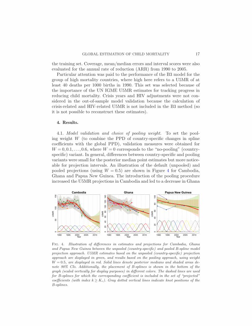
4.1. Model validation and choice of pooling weight. To set the pool-ing weight W (to combine the PPD of country-specific changes in splinecoefficients with the global PPD), validation measures were obtained forW = 0,0.1, . . . ,0.6, where W = 0 corresponds to the “no-pooling” (country-specific) variant. In general, differences between country-specific and poolingvariants were small for the posterior median point estimates but more notice-able for projection intervals. An illustration of the default (unpooled) andpooled projections (using W = 0.5) are shown in Figure 4 for Cambodia,Ghana and Papua New Guinea. The introduction of the pooling procedureincreased the U5MR projections in Cambodia and led to a decrease in Ghana

Fig. 4. Illustration of differences in estimates and projections for Cambodia, Ghanaand Papua New Guinea between the unpooled (country-specific) and pooled B-spline modelprojection approach. U5MR estimates based on the unpooled (country-specific) projectionapproach are displayed in green, and results based on the pooling approach, using weightW = 0.5, are displayed in red. Solid lines denote posterior medians and shaded areas de-note 90% CIs. Additionally, the placement of B-splines is shown in the bottom of thegraph (scaled vertically for display purposes) in different colors. The dashed lines are usedfor B-splines for which the corresponding coefficient is included in the set of “projected”coefficients (with index k ≥Kc). Gray dotted vertical lines indicate knot positions of theB-splines.

18 L. ALKEMA AND J. R. NEW

and Papua New Guinea, but differences in point estimates were minor. Pro-jection intervals varied more across countries; the bounds were similar forweights 0 and 0.5 for Ghana, but narrowed down in Cambodia and werelower for the pooled projections in Papua New Guinea.

Model validation results based on the left-out observations and the com-parison between estimates based on the training and full data set are shownin Tables 2, 3 and 4 in the Appendix for the range of pooling weights. Differ-ences in mean/median (absolute) errors were small. While for median errorsthe comparison across the different weights varied by indicator, mean errorsgenerally decreased with increasing pooling weights. Coverage and intervalwidth scores for left-out observations generally improved slightly with in-creasing pooling weight. For the estimated U5MR and ARR, findings oncoverage of 90% credible intervals were mixed, but mean interval scores forU5MR decreased with increasing pooling weight.

Based on these findings, we chose to apply the pooling. Because differencesin validation outcomes were small when comparing the results for W = 0.5 tothose with W = 0.6, and because of the convenient interpretation of W = 0.5(the projected mean and variance of the differences in the spline coefficientsare the simple average of the country-specific and global estimates), we setW = 0.5. A comparison of estimates and short-term projections based onW = 0 and W = 0.5 for all countries is included in supplementary Figure S1[Alkema and New (2014)].

With this choice of W , the model validation results for the B3 modelshowed an improvement over those for the UN IGME 2012 estimation ap-proach. In a similar validation exercise carried out for the UN IGME 2012estimation approach [Alkema and New (2012)], the updated estimate of ARRfor 1990–2005 (based on the full data set) was above the training 90% CI for16% of the high mortality countries (11 out of 70 countries) and below thatfor only 6% of those countries. This indicates that declines in U5MR wereunderestimated for a substantial proportion of high mortality countries. Thesame effect is observed in the validation results for the B3 model but to amuch lesser extent, with only 9% of the updated upper bounds for the ARRbeing too low and 3% of the updated lower bounds being too high. Overall,the calibration measures are better with the B3 model. Specifically, the per-centages of updated estimates falling below and above the 90% uncertaintyintervals were 4% and 5%, respectively, for the U5MR in 2000 and 8% and1% for the U5MR in 2005 in the B3 model. These percentages were 10%and 6% for the U5MR in 2000 and 17% and 7% for the U5MR in 2005 inthe IGME 2012 estimation approach.

4.2. Data model biases. Mean biases in U5MR levels and trends, as wellas 90% prediction intervals for the expected range of U5MR values, werecalculated based on the posterior sample of data quality parameters and

GLOBAL ESTIMATION OF CHILD MORTALITY 19

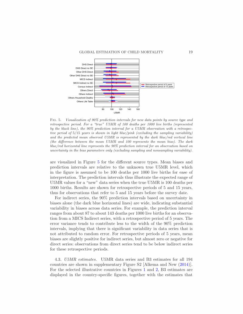
Fig. 5. Visualization of 90% prediction intervals for new data points by source type andretrospective period. For a “true” U5MR of 100 deaths per 1000 live births (representedby the black line), the 90% prediction interval for a U5MR observation with a retrospec-tive period of 5/15 years is shown in light blue/pink (excluding the sampling variability)and the predicted mean observed U5MR is represented by the dark blue/red vertical line(the difference between the mean U5MR and 100 represents the mean bias). The darkblue/red horizontal line represents the 90% prediction interval for an observation based onuncertainty in the bias parameters only (excluding sampling and nonsampling variability).

are visualized in Figure 5 for the different source types. Mean biases andprediction intervals are relative to the unknown true U5MR level, whichin the figure is assumed to be 100 deaths per 1000 live births for ease ofinterpretation. The prediction intervals thus illustrate the expected range ofU5MR values for a “new” data series when the true U5MR is 100 deaths per1000 births. Results are shown for retrospective periods of 5 and 15 years,thus for observations that refer to 5 and 15 years before the survey date.

For indirect series, the 90% prediction intervals based on uncertainty inbiases alone (the dark blue horizontal lines) are wide, indicating substantialvariability in biases across data series. For example, the prediction intervalranges from about 87 to about 143 deaths per 1000 live births for an observa-tion from a MICS Indirect series, with a retrospective period of 5 years. Theerror variance tends to contribute less to the width of the 90% predictionintervals, implying that there is significant variability in data series that isnot attributed to random error. For retrospective periods of 5 years, meanbiases are slightly positive for indirect series, but almost zero or negative fordirect series: observations from direct series tend to be below indirect seriesfor these retrospective periods.

4.3. U5MR estimates. U5MR data series and B3 estimates for all 194countries are shown in supplementary Figure S2 [Alkema and New (2014)].For the selected illustrative countries in Figures 1 and 2, B3 estimates aredisplayed in the country-specific figures, together with the estimates that

20 L. ALKEMA AND J. R. NEW

would have been obtained using the default Loess estimation approach usedfor constructing the IGME 2012 estimates.

Point estimates from the B3 model and default Loess are almost identicalfor the Netherlands during the entire observation period, but differ for all ora subset of observation years in the other countries. For Mexico, the trendin the Loess estimates for the late 2000s contradicts the observed trend inVR data. B3 estimates take into account the small stochastic error in theVR and follow the data points closely. For Moldova, the inclusion of the VRobservations in the early 1990s with a VR bias parameter for those years re-sults in U5MR estimates that capture the VR-indicated trend. The inclusionof VR data for recent years guarantees that the point estimates and credibleintervals do not cross through the VR. In future revisions for Moldova, afurther extension could be to include all incomplete VR observations as aminimum to avoid the situation in the early 1980s, when the lower boundof the CI is below the incomplete VR.

For Ghana, B3 estimates and Loess estimates are similar. Small differ-ences are observed in the years with VR data, where the B3 estimatescapture these points while the Loess does not. In more recent years, theextrapolated decline is slightly steeper for the B3 model, as indicated by thedecline in the most recent observations. Differences between B3 and Loessestimates are much larger in the other countries in the figure. In Cambodia,the B3 estimates follow the trend as observed in the data series, includ-ing the stagnation of child mortality decline in the 1980s and 1990s andthe more recent acceleration in the decline of child mortality. The defaultLoess fit does not capture these fluctuations. In the IGME 2012 method,this country would be a candidate for an expert-based adjustment of theLoess smoothing parameter to better capture the trend. In the B3 penalizedspline model approach, such expert adjustments are not necessary.

In Pakistan, the B3 estimates follow the registration data. The DHS from2006–2007 does not bias downward the estimates (as observed in the Loessestimates) because of the inclusion of bias parameters for survey data; weestimate that the DHS Direct series is biased downward. Last, in PNG, B3estimates suggest a slightly flatter trend in U5MR than the Loess duringthe 1980s and 1990s based on the lack of downward trends in all individualseries during that period.

5. Discussion. The estimation of child mortality is challenging for thegreat majority of developing countries without well-functioning VR systemsdue to issues with data quantity and quality. In this paper, we described aBayesian penalized B-spline regression model to evaluate levels and trendsin the U5MR for all countries in the world. This model estimates biases indata series for all non-VR source types using a multilevel model to improveupon the limitations of current methods. Improved spline extrapolations are

GLOBAL ESTIMATION OF CHILD MORTALITY 21

obtained via logarithmic pooling of the posterior predictive distribution ofcountry-specific changes in spline coefficients with observed changes on theglobal level. The proposed model can flexibly capture changes in U5MR overtime, provides point estimates and credible intervals that take into consider-ation potential biases in data series and gives better model validation resultsthan the UN IGME 2012 estimation approach.

The differences between the B3 estimates and the default Loess fits asdiscussed in Section 4.3 highlight the need for more attention for appropriatedata models in U5MR estimation. When treating all observations equally,U5MR estimates can end up below (incomplete) VR observations or followa trend in U5MR that is dictated by the (lack of) overlap of different dataseries with potentially different level biases.

While our data model overcomes the main limitations of the previous UNIGME estimation methods, there remains room for improvement. The pri-mary issue with child mortality estimation is data quality. In the B3 datamodel, we incorporated source-specific bias parameters, that are drawn froma source type-specific distribution based on the assumption that biases arecomparable across data series of the same source type. However, large varia-tion exists across series; ideally, external information on data quality shouldbe included to distinguish between the more or less reliable series in thedatabase. In a residual analysis, (absolute) residuals were plotted againsta number of data quality predictors (region that country belongs to, se-ries source type, series year, observation year, retrospective period, level ofU5MR in observation year, total fertility rate in the series year and changein the total fertility rate in the last 15 years before the series) to explorewhether any of those covariates should be incorporated into the model forbiases in direct and indirect series. Overall, the linear model without covari-ates seemed to work reasonably well except for some DHS Direct series, forwhich an additional negative bias for observations with retrospective periodsshorter than 5 years may be present. This may be due to birth transference,whereby dates of birth are incorrectly reported to avoid answering morequestions pertaining to those births in the DHS questionnaires [Sullivan(2008)]. Given the importance of the observations with short retrospectiveperiods in driving recent estimates and short-term projections, this issueneeds to be investigated more in future work.

Improved spline extrapolations were obtained via logarithmic pooling ofthe posterior predictive distribution of country-specific changes in splinecoefficients with observed changes on the global level. While short-term pro-jections that are based only on country-specific information may be pre-ferred from a political/country-user point of view, the pooling procedurewas used because it was found to improve out-of-sample model performanceand deemed to lead to more plausible projection intervals in countries where

22 L. ALKEMA AND J. R. NEW

differences between the pooled and unpooled predictions occurred. In sum-mary, the pooling approach reduces the probability of unrealistically highor low rates of changes in extrapolations and also reduces the probabilityof sustained high or low rates of change over longer projection periods bypooling the predictive distribution for rates of change toward a global distri-bution. This procedure did not result in large differences in point estimatesfor the majority of countries (as illustrated in Figure S1); its main effect wasa reduction of upper bounds for the U5MR by reducing the probability ofvery low or even negative rates of change. Alternative projection methodsmay be considered, for example, based on country-specific covariates whichmay be informative of U5MR declines. However, given the limited avail-ability of such covariates for recent years, we did not pursue this researchdirection.

Ultimately, the issues of data quality and availability of more recent datacan only be resolved by implementing fully functioning VR systems thatcan provide accurate data on births and deaths in every country. However,currently only about 50 countries have such VR systems in place; the imple-mentation of VR systems for all countries remains an ambitious and long-term goal [United Nations Children’s Fund and USAID (2012)]. In the shortterm, the B3 model allows for inclusion of information from incomplete VRsystems, as illustrated for Moldova. The inclusion of data from alternativedata sources and the implementation of novel data collection methods, thatcan provide accurate and timely child mortality data [e.g., see Clark et al.(2012) and Amouzou (2011)], could further aid child mortality estimation.The advantage of the use of the Bayesian framework in the B3 model is thatthe model can be readily extended to incorporate such information into theestimation process.

To assess progress toward MDG 4, much focus is placed on the point es-timates of the U5MR and ARR despite the large uncertainty in estimatesbecause communication of uncertainty in U5MR estimates is challenging[Oestergaard, Alkema and Lawn (2013)]. To provide a straightforward in-clusion of the uncertainty assessment into the MDG 4 progress assessment,countries could be categorized by whether the attainment of the MDG tar-get of an ARR of 4.4% is considered to be unlikely, not clear or likely basedon the uncertainty intervals of the ARR estimate [Alkema and New (2012)].

Moving beyond the MDGs, the issue of inequality is likely to featureprominently in the post-2015 development agenda. While the MDGs havefocused much attention on national, regional and global averages of keyindicators, they have also potentially masked growing disparities at the intra-national level [UN System Task Team on the Post-2015 UN DevelopmentAgenda (2012)]. In light of this, disaggregated estimates of child mortality(e.g., by state, wealth quintile, residence) will be increasingly importantto evaluate progress for all population groups to better address inequalities.

GLOBAL ESTIMATION OF CHILD MORTALITY 23

Further work can be carried out to extend the B3 model so that this growingbody of disaggregated data can be fully utilized to produce disaggregated

estimates in the future.

APPENDIX

Prior distributions. Prior distributions for the spline model parametersare specified as follows:

exp(λc,0)∼ U(1,1000),

λc,1/I ∼ U(−0.25,0.2),

χ∼N(−3,10),

ϕ∼ U(0,5),

where exp(λc,0) represents the level of U5MR in the approximate midyear ofthe observation period, and λc,1/I is approximately the average ARR over

the observation period (I is the interval length between knots).Diffuse prior distributions were assigned to all data model parameters,

with the exception of the mean bias µ0,d for the DHS Direct series, which

has an informative prior distribution:

µ0,d ∼N(M0,d, S20,d),

µ1,d ∼N(M1,d, S21,d),

φ0,d ∼ U(0,5),

φ1,d ∼ U(0,5),

ωd′ ∼ U(0,0.5),

where M0,d =−0.0123 for d= DHS direct and 0 otherwise, M1,d = 0 for alld, S0,d = 0.00556 for DHS Direct and 0.15 otherwise, S1,d = 0.02 for all d.

Logarithmic pooling approach. The penalized spline model-induced PPD

for γ(j)c,Kc

=∆α(j)c,Kc

= α(j)c,Kc

−α(j)c,Kc−1, based on (4), is given by

γ(j)c,Kc

|γ(j)c,Kc−1,Θ

(j)c,Kc

∼N(γ(j)c,Kc−1,Θ

(j)c,Kc

),(7)

where Θ(j)c,Kc

= (σ2c )

(j). Its density function (leaving out superscripts to de-

note the posterior sample for notational convenience) p∗(γc,Kc) = f(γc,Kc

|

γc,Kc−1,Θc,Kc), where f(Γ|µ,σ2) denotes the probability density function

for a normal random variable with mean µ and variance σ2.

24 L. ALKEMA AND J. R. NEW

The model-induced PPD is pooled with a (direct) global PPD for futurechanges in the spline coefficients, which was based on the set of posterior

median estimates of the γ(j)c,k ’s, γc,k for c = 1, . . . ,C and k = 2, . . . ,Kc − 1

(during the observation period for each country):

p(γ) = f(γ|G,V ),(8)

where G and V were given by the median and variance of the γc,k’s, respec-tively.

Logarithmic pooling is used to combine both density functions:

p(Γc,Kc)∝ p∗(γc,Kc

)1−wc,Kc · p(γc,Kc)wc,Kc = f(γc,Kc

|Γc,Kc,Θc,Kc

),

where wc,Kcis the country-projection-step specific logarithmic pooling weight

that determines the extent of pooling,

wc,Kc=

W · V

W · V + (1−W )Θc,Kc−1,

with overall weight 0≤W ≤ 1 such that

Γc,Kc=W ·G+ (1−W ) · γc,Kc−1,

Θc,Kc=W · V + (1−W ) ·Θc,Kc−1.

For a≥ 1, the induced PPD is defined as

p∗(γc,Kc+a) = f(γc,Kc+a|Γc,Kc+a−1,Θc,Kc+a−1).

With the global distribution from equation(8) and logarithmic poolingweights wc,Kc+a =

W ·VW ·V+(1−W )Θc,Kc+a−1

, the pooled distribution for γc,Kc+a

is given by

p(γc,Kc+a)∝ p∗(γc,Kc+a)1−wc,Kc+a · p(γc,Kc+a)

wc,Kc+a

= f(γc,Kc+a|Γc,Kc+a,Θc,Kc+a),

Γc,Kc+a =W ·G+ (1−W ) · γc,Kc+a−1,

Θc,Kc+a =W · V + (1−W ) ·Θc,Kc+a−1.

Validation results. Validation results are described in Tables 2, 3 and 4.

Acknowledgments. The authors are very grateful to all members of the(Technical Advisory Group of the) United Nations Inter-agency Group forChild Mortality Estimation for passionate discussions about U5MR dataand preliminary B3 estimates which have greatly improved this work. Ad-ditional thanks to Danzhen You, Patrick Gerland, Simon Cousens, KennethHill, Kirill Andreev, Francois Pelletier, Bruno Masquelier, David Nott, An-

GLOBAL ESTIMATION OF CHILD MORTALITY 25

Table 2

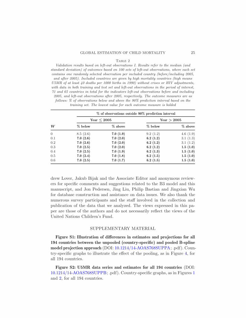
Validation results based on left-out observations I. Results refer to the median (andstandard deviation) of outcomes based on 100 sets of left-out observations, where each setcontains one randomly selected observation per included country (before/including 2005,and after 2005). Included countries are given by high mortality countries (high means

U5MR of at least 40 deaths per 1000 births in 1990) without crises or HIV adjustments,with data in both training and test set and left-out observations in the period of interest,71 and 65 countries in total for the indicators left-out observations before and including2005, and left-out observations after 2005, respectively. The outcome measures are asfollows: % of observations below and above the 90% prediction interval based on the

training set. The lowest value for each outcome measure is bolded

% of observations outside 90% prediction interval

Year ≤ 2005 Year > 2005

W % below % above % below % above

0 8.5 (2.6) 7.0 (1.9) 9.2 (1.2) 4.6 (1.9)0.1 7.0 (2.6) 7.0 (2.0) 6.2 (1.2) 3.1 (1.3)0.2 7.0 (2.6) 7.0 (2.0) 6.2 (1.2) 3.1 (1.2)0.3 7.0 (2.5) 7.0 (2.0) 6.2 (1.2) 1.5 (1.0)0.4 7.0 (2.5) 7.0 (1.9) 6.2 (1.3) 1.5 (1.0)0.5 7.0 (2.4) 7.0 (1.8) 6.2 (1.5) 1.5 (1.0)0.6 7.0 (2.5) 7.0 (1.7) 6.2 (1.5) 1.5 (1.0)

drew Lover, Jakub Bijak and the Associate Editor and anonymous review-ers for specific comments and suggestions related to the B3 model and thismanuscript, and Jon Pedersen, Jing Liu, Philip Bastian and Jingxian Wufor database construction and assistance on data issues. We also thank thenumerous survey participants and the staff involved in the collection andpublication of the data that we analyzed. The views expressed in this pa-per are those of the authors and do not necessarily reflect the views of theUnited Nations Children’s Fund.

SUPPLEMENTARY MATERIAL

Figure S1: Illustration of differences in estimates and projections for all194 countries between the unpooled (country-specific) and pooled B-splinemodel projection approach (DOI: 10.1214/14-AOAS768SUPPA; .pdf). Coun-try-specific graphs to illustrate the effect of the pooling, as in Figure 4, forall 194 countries.

Figure S2: U5MR data series and estimates for all 194 countries (DOI:10.1214/14-AOAS768SUPPB; .pdf). Country-specific graphs, as in Figures 1and 2, for all 194 countries.

26 L. ALKEMA AND J. R. NEW

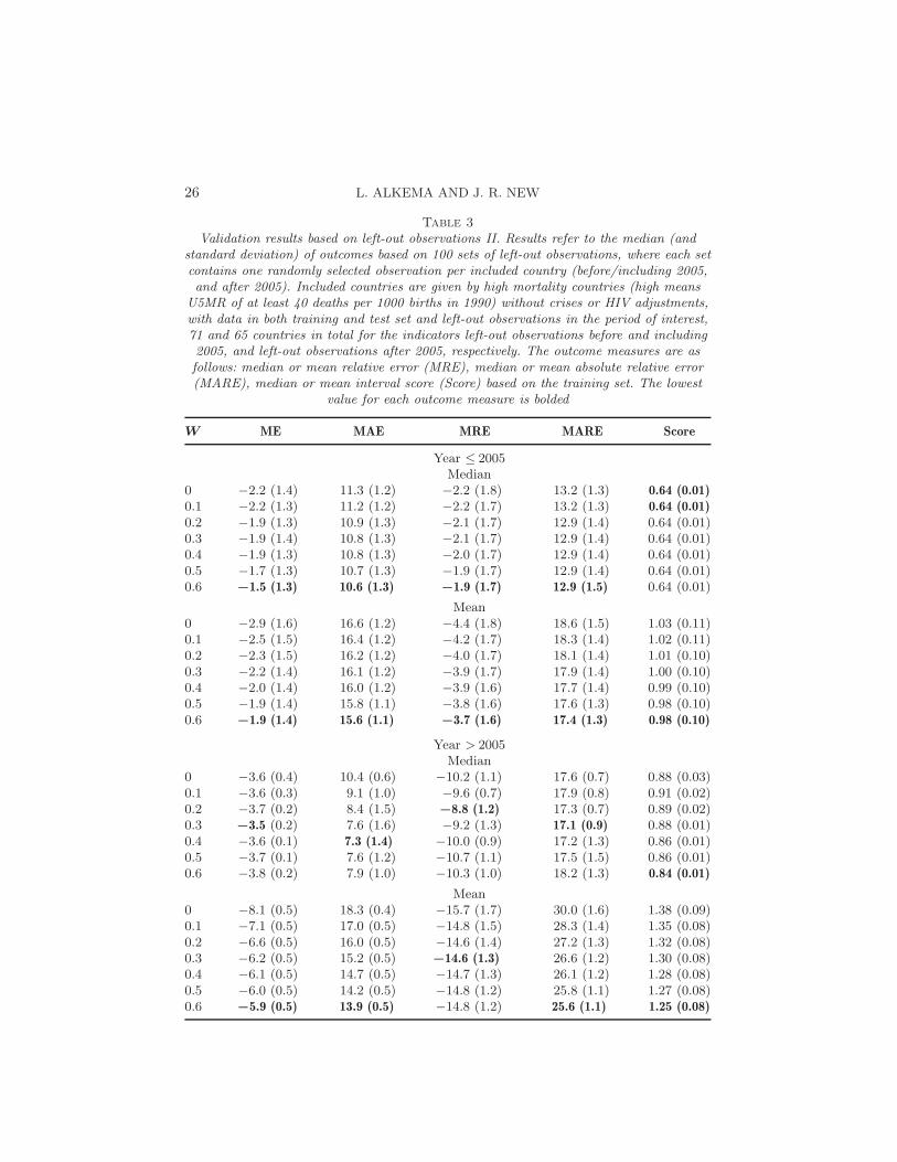
Table 3

Validation results based on left-out observations II. Results refer to the median (andstandard deviation) of outcomes based on 100 sets of left-out observations, where each setcontains one randomly selected observation per included country (before/including 2005,and after 2005). Included countries are given by high mortality countries (high means

U5MR of at least 40 deaths per 1000 births in 1990) without crises or HIV adjustments,with data in both training and test set and left-out observations in the period of interest,71 and 65 countries in total for the indicators left-out observations before and including2005, and left-out observations after 2005, respectively. The outcome measures are asfollows: median or mean relative error (MRE), median or mean absolute relative error(MARE), median or mean interval score (Score) based on the training set. The lowest

value for each outcome measure is bolded

W ME MAE MRE MARE Score

Year ≤ 2005Median

0 −2.2 (1.4) 11.3 (1.2) −2.2 (1.8) 13.2 (1.3) 0.64 (0.01)0.1 −2.2 (1.3) 11.2 (1.2) −2.2 (1.7) 13.2 (1.3) 0.64 (0.01)0.2 −1.9 (1.3) 10.9 (1.3) −2.1 (1.7) 12.9 (1.4) 0.64 (0.01)0.3 −1.9 (1.4) 10.8 (1.3) −2.1 (1.7) 12.9 (1.4) 0.64 (0.01)0.4 −1.9 (1.3) 10.8 (1.3) −2.0 (1.7) 12.9 (1.4) 0.64 (0.01)0.5 −1.7 (1.3) 10.7 (1.3) −1.9 (1.7) 12.9 (1.4) 0.64 (0.01)0.6 −1.5 (1.3) 10.6 (1.3) −1.9 (1.7) 12.9 (1.5) 0.64 (0.01)

Mean0 −2.9 (1.6) 16.6 (1.2) −4.4 (1.8) 18.6 (1.5) 1.03 (0.11)0.1 −2.5 (1.5) 16.4 (1.2) −4.2 (1.7) 18.3 (1.4) 1.02 (0.11)0.2 −2.3 (1.5) 16.2 (1.2) −4.0 (1.7) 18.1 (1.4) 1.01 (0.10)0.3 −2.2 (1.4) 16.1 (1.2) −3.9 (1.7) 17.9 (1.4) 1.00 (0.10)0.4 −2.0 (1.4) 16.0 (1.2) −3.9 (1.6) 17.7 (1.4) 0.99 (0.10)0.5 −1.9 (1.4) 15.8 (1.1) −3.8 (1.6) 17.6 (1.3) 0.98 (0.10)0.6 −1.9 (1.4) 15.6 (1.1) −3.7 (1.6) 17.4 (1.3) 0.98 (0.10)

Year > 2005Median

0 −3.6 (0.4) 10.4 (0.6) −10.2 (1.1) 17.6 (0.7) 0.88 (0.03)0.1 −3.6 (0.3) 9.1 (1.0) −9.6 (0.7) 17.9 (0.8) 0.91 (0.02)0.2 −3.7 (0.2) 8.4 (1.5) −8.8 (1.2) 17.3 (0.7) 0.89 (0.02)0.3 −3.5 (0.2) 7.6 (1.6) −9.2 (1.3) 17.1 (0.9) 0.88 (0.01)0.4 −3.6 (0.1) 7.3 (1.4) −10.0 (0.9) 17.2 (1.3) 0.86 (0.01)0.5 −3.7 (0.1) 7.6 (1.2) −10.7 (1.1) 17.5 (1.5) 0.86 (0.01)0.6 −3.8 (0.2) 7.9 (1.0) −10.3 (1.0) 18.2 (1.3) 0.84 (0.01)

Mean0 −8.1 (0.5) 18.3 (0.4) −15.7 (1.7) 30.0 (1.6) 1.38 (0.09)0.1 −7.1 (0.5) 17.0 (0.5) −14.8 (1.5) 28.3 (1.4) 1.35 (0.08)0.2 −6.6 (0.5) 16.0 (0.5) −14.6 (1.4) 27.2 (1.3) 1.32 (0.08)0.3 −6.2 (0.5) 15.2 (0.5) −14.6 (1.3) 26.6 (1.2) 1.30 (0.08)0.4 −6.1 (0.5) 14.7 (0.5) −14.7 (1.3) 26.1 (1.2) 1.28 (0.08)0.5 −6.0 (0.5) 14.2 (0.5) −14.8 (1.2) 25.8 (1.1) 1.27 (0.08)0.6 −5.9 (0.5) 13.9 (0.5) −14.8 (1.2) 25.6 (1.1) 1.25 (0.08)

GLOBAL ESTIMATION OF CHILD MORTALITY 27

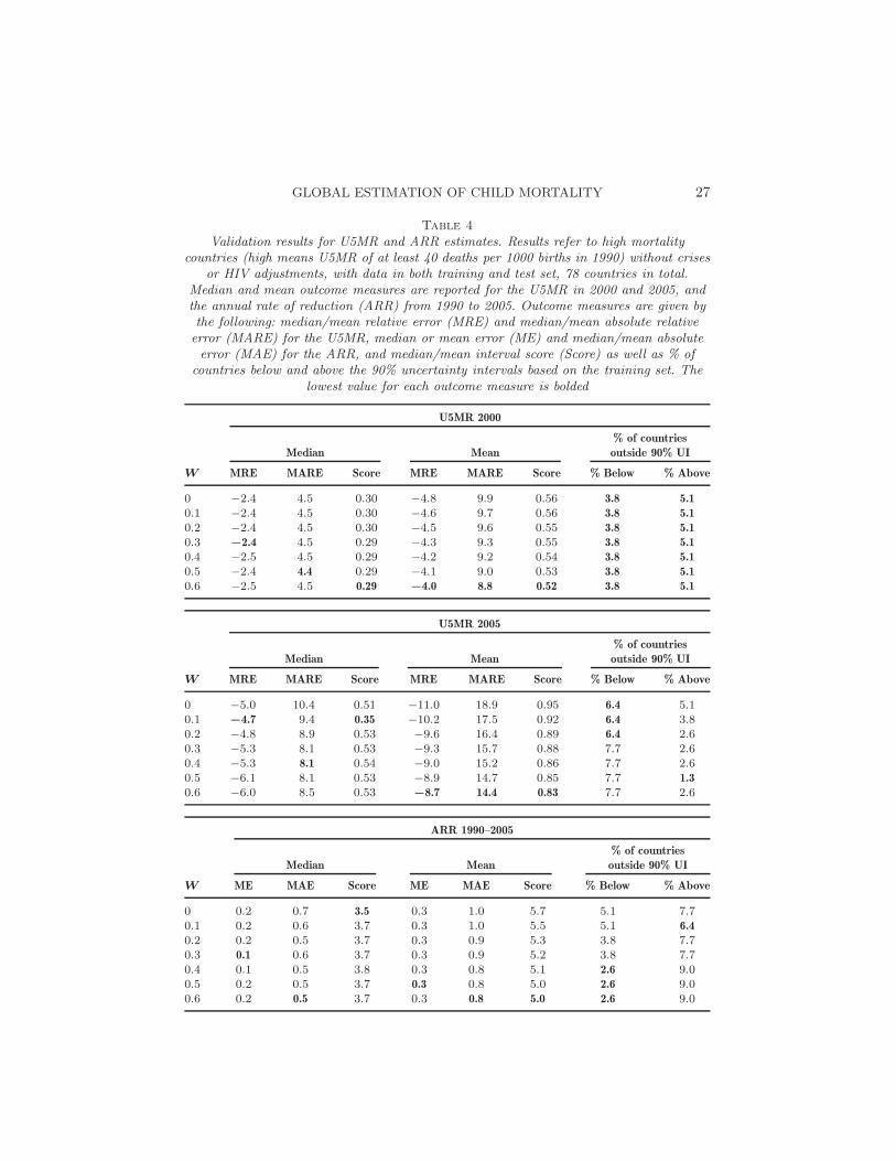
Table 4

Validation results for U5MR and ARR estimates. Results refer to high mortalitycountries (high means U5MR of at least 40 deaths per 1000 births in 1990) without crises

or HIV adjustments, with data in both training and test set, 78 countries in total.Median and mean outcome measures are reported for the U5MR in 2000 and 2005, andthe annual rate of reduction (ARR) from 1990 to 2005. Outcome measures are given bythe following: median/mean relative error (MRE) and median/mean absolute relativeerror (MARE) for the U5MR, median or mean error (ME) and median/mean absoluteerror (MAE) for the ARR, and median/mean interval score (Score) as well as % of

countries below and above the 90% uncertainty intervals based on the training set. Thelowest value for each outcome measure is bolded

U5MR 2000

% of countries

Median Mean outside 90% UI

W MRE MARE Score MRE MARE Score % Below % Above

0 −2.4 4.5 0.30 −4.8 9.9 0.56 3.8 5.1

0.1 −2.4 4.5 0.30 −4.6 9.7 0.56 3.8 5.1

0.2 −2.4 4.5 0.30 −4.5 9.6 0.55 3.8 5.1

0.3 −2.4 4.5 0.29 −4.3 9.3 0.55 3.8 5.1

0.4 −2.5 4.5 0.29 −4.2 9.2 0.54 3.8 5.1

0.5 −2.4 4.4 0.29 −4.1 9.0 0.53 3.8 5.1

0.6 −2.5 4.5 0.29 −4.0 8.8 0.52 3.8 5.1

U5MR 2005

% of countries

Median Mean outside 90% UI

W MRE MARE Score MRE MARE Score % Below % Above

0 −5.0 10.4 0.51 −11.0 18.9 0.95 6.4 5.10.1 −4.7 9.4 0.35 −10.2 17.5 0.92 6.4 3.80.2 −4.8 8.9 0.53 −9.6 16.4 0.89 6.4 2.60.3 −5.3 8.1 0.53 −9.3 15.7 0.88 7.7 2.60.4 −5.3 8.1 0.54 −9.0 15.2 0.86 7.7 2.60.5 −6.1 8.1 0.53 −8.9 14.7 0.85 7.7 1.3

0.6 −6.0 8.5 0.53 −8.7 14.4 0.83 7.7 2.6

ARR 1990–2005

% of countries

Median Mean outside 90% UI

W ME MAE Score ME MAE Score % Below % Above

0 0.2 0.7 3.5 0.3 1.0 5.7 5.1 7.70.1 0.2 0.6 3.7 0.3 1.0 5.5 5.1 6.4

0.2 0.2 0.5 3.7 0.3 0.9 5.3 3.8 7.70.3 0.1 0.6 3.7 0.3 0.9 5.2 3.8 7.70.4 0.1 0.5 3.8 0.3 0.8 5.1 2.6 9.00.5 0.2 0.5 3.7 0.3 0.8 5.0 2.6 9.00.6 0.2 0.5 3.7 0.3 0.8 5.0 2.6 9.0

28 L. ALKEMA AND J. R. NEW

REFERENCES

Alkema, L. and New, J. R. (2012). Progress toward global reduction in under-five mor-tality: A bootstrap analysis of uncertainty in Millennium Development Goal 4 estimates.PLoS Med. 9 e1001355.

Alkema, L. and New, J. R. (2013). Global estimation of child mortality using a BayesianB-spline bias-reduction model. Technical report. Available at http://arxiv.org/abs/1309.1602.

Alkema, L. and New, J. (2014). Supplement to “Global estimation of child mortalityusing a Bayesian B-spline Bias-reduction model.” DOI:10.1214/14-AOAS768SUPPA,DOI:10.1214/14-AOAS768SUPPB.

Alkema, L., Wong, M. B. and Seah, P. R. (2012). Monitoring progress towards Mil-lennium Development Goal 4: A call for improved validation of under-5 mortality rateestimates. Statistics, Politics and Policy 3 Article ID 2.

Amouzou, A. (2011). Real-time results tracking. Technical report, Institute forInternational Programs, Johns Hopkins Bloomberg School of Public Healt, Balti-more. Available at http://www.jhsph.edu/departments/international-health/

centers-and-institutes/institute-for-international-programs/_documents/

RRT_Technical_Note.pdf.Brass, W. (1964). Uses of census or survey data for the estimation of vital rates. In

African Seminar on Vital Statistics, 14–19 December 1964, United Nations, New York.Census of India (2011). Sample registration. Available at http://censusindia.gov.in/

Vital_Statistics/SRS/Sample_Registration_System.aspx.Clark, S. J., Wakefield, J., McCormick, T. and Ross, M. (2012). Hyak mortality

monitoring system: Innovative sampling and estimation methods. Working Paper 118.Available at http://www.csss.washington.edu/Papers/wp118.pdf.

Currie, I. D. and Durban, M. (2002). Flexible smoothing with P -splines: A unifiedapproach. Stat. Model. 2 333–349. MR1951589

Eilers, P. H. C. (1999). Discussion of “The analysis of designed experiments and longi-tudinal data using smoothing splines” by A. P. Verbyla, B. R. Cullis, M. G. Kenwardand S. J. Welham. J. R. Stat. Soc. Ser. C. Appl. Stat. 48 300–311.

Eilers, P. H. C. and Marx, B. D. (1996). Flexible smoothing with B-splines and penal-ties. Statist. Sci. 11 89–121. MR1435485

Eilers, P. H. C. and Marx, B. D. (2010). Splines, knots, and penalties. Wiley Interdis-ciplinary Reviews: Computational Statistics 2 637–653.

Gelman, A. and Rubin, D. (1992). Inference from iterative simulation using multiplesequences. Statist. Sci. 7 457–511.

Gneiting, T. and Raftery, A. E. (2007). Strictly proper scoring rules, prediction, andestimation. J. Amer. Statist. Assoc. 102 359–378. MR2345548

Hill, K., You, D., Inoue, M. and Oestergaard, M. Z. (2012). Child mortality estima-tion: Accelerated progress in reducing global child mortality PLoS Med. 9 e1001303.

Oestergaard, M. Z., Alkema, L. and Lawn, J. E. (2013). Millennium DevelopmentGoals national targets are moving targets and the results will not be known until wellafter the deadline of 2015. International Journal of Epidemiology 42 645–647.

Pedersen, J. and Liu, J. (2012). Child mortality estimation: Appropriate time periodsfor child mortality estimates from full birth histories. PLoS Med. 9 e1001289.

Plummer, M. (2003). JAGS: A program for analysis of Bayesian graphical models usingGibbs sampling. In Proceedings of the 3rd International Workshop on Distributed Sta-tistical Computing (DSC 2003), Vienna. Available at http://mcmc-jags.sourceforge.net/.

GLOBAL ESTIMATION OF CHILD MORTALITY 29

Raftery, A. E. and Lewis, S. M. (1992). How many iterations in the Gibbs sampler?In Bayesian Statistics 4 (J. M. Bernardo et al., eds.) 763–773. Oxford Univ. Press,Oxford.

Raftery, A. E and Lewis, S. M. (1996). Implementing MCMC. In Markov Chain MonteCarlo in Practice (W. R. Gilks, D. J. Spiegelhalter and S. Richardson, eds.) 115–130. Chapman & Hall, London. MR1397966

Rajaratnam, J. K., Marcus, J., Flaxman, A., Wang, H., Levin-Rector, A.,Dwyer, L., Costa, M., Lopez, A. and Murray, C. (2010). Neonatal, postneonatal,childhood, and under-5 mortality for 187 countries, 1970–2010: A systematic analysisof progress towards Millennium Development Goal 4. The Lancet 375 1988–2008.

Sullivan, J. M. (2008). An assessment of the credibility of child mortality declinesestimated from DHS mortality rates. Working Paper 1, United Nations Children’sFund, New York. Available at http://www.childinfo.org/files/Overall_Results_

of_Analysis.pdf.UN System Task Team on the Post-2015 UN Development Agenda (2012). Addressing

inequalities: The heart of the post-2015 agenda and the future we want for all. Availableat http://www.un.org/millenniumgoals/pdf/10_inequalities_20July.pdf.

United Nations (1983). Manual X: Indirect Techniques for Demographic Estimation.United Nations, New York.

United Nations Children’s Fund and USAID (2012). Real-time childmortality monitoring meeting. United Nations Children’s Fund,New York. Available at http://newsletter.childrenandaids.org/

real-time-child-mortality-monitoring-meeting-december-19-2012/ .United Nations Children’s Fund, Division of Policy and Strategy (2013). Committing

to child survival: A promise renewed progress report 2013. United Nations Children’sFund, New York.

United Nations, Department of Economic and Social Affairs, Population Division (2011).World population prospects. The 2010 Revision.

Wang, H., Dwyer-Lindgren, L., Lofgren, K. T., Rajaratnam, J. K., Mar-

cus, J. R., Levin-Rector, A., Levitz, C. E., Lopez, A. D. and Murray, C. J.

(2012). Age-specific and sex-specific mortality in 187 countries, 1970–2010: A system-atic analysis for the global burden of disease study 2010. The Lancet 380 2071–2094.

United Nations Inter-Agency Group for Child Mortality Estimation (2012). Levels &trends in child mortality: Report 2012. United Nations Children’s Fund, New York.

United Nations Inter-Agency Group for Child Mortality Estimation (2013). Levels &trends in child mortality: Report 2013. United Nations Children’s Fund, New York.

Department of Statistics and Applied Probability

National University of Singapore

Blk S16, Level 7, 6

Science Drive 2

Singapore 117546

Singapore

E-mail: alkema@nus.edu.sgjrnew@nus.edu.sg