National Policy for Regional Development:Evidence from Appalachian Highways∗

Taylor Jaworski† Carl T. Kitchens‡

September 10, 2016

Abstract

How effective are policies aimed at integrating isolated regions? We answer thisquestion using the construction of a highway system in one of the poorest regions inthe United States. With construction starting in 1965, the Appalachian DevelopmentHighway System (ADHS) ultimately consisted of over 2,500 high-grade road miles.Motivated by a model of interregional trade we estimate the elasticity of total incomewith respect to market access, which we then use to evaluate the overall impact ofthe ADHS. We find that removing the ADHS would have reduced the total income by$30.1 billion or, roughly, 3.4 percent in the targeted region. Ultimately, the populationresponse to improvements in transportation infrastructure reduced the gains in incomeper capita, which were equal to $586 annually in the poorest counties. Today, theregion’s performance relative to the national average is similar to its position in the1960s; despite substantial investment in transportation and some gains in income percapita, the region continues to lag behind the rest of the country.

∗We thank Jeremy Atack, Nate Baum-Snow, Bill Collins, Price Fishback, Walker Hanlon, Josh Hausman,Rick Hornbeck, Shawn Kantor, Ian Keay, Frank Lewis, Gary Libecap, John Wallis, Alex Whalley andconference/seminar participants at the 2015 Canadian Network for Economic History meetings, Colgate,Lakehead, McGill, York, and the 2016 NBER Summer Institute (DAE) for comments that improved thepaper. All remaining errors are our own.†Queen’s University, Department of Economics, (tjaworski@gmail.com)‡Florida State University, Department of Economics, (ckitchens@fsu.edu)

1 Introduction

There are large differences in economic performance and individual outcomes across space

within the United States and elsewhere. The integration of regions with the national econ-

omy may facilitate growth through increased trading opportunities with the rest of the

country or increased productivity due to competition and the transfer of frontier technology

to underdeveloped regions. At the same time, policymakers must balance concerns at the

national level with policies that disproportionately benefit (or harm) particular regions. In

the context of the United States, the counties in and around the Appalachian Mountains are

among the poorest in the country with income per capita more than 20 percent below the

national average.

In the early 1960s, the stark contrast between Appalachia and the rest of the country

led the region’s governors to lobby the federal government for relief. In 1965, President

Johnson signed the Appalachian Regional Development Act, creating the Appalachian Re-

gional Commission (ARC)–a federal-state partnership aimed at integrating the region–and

fulfilling promises made by the Kennedy Administration. To date, over $34 billion (in 2015

dollars) of federal expenditures have gone to the region, with the bulk of funding going to the

construction of the nearly 2,500 miles of the Appalachian Development Highway System.1

The construction of the Appalachian Development Highway System provides an opportunity

to study the long-run impact of a policy aimed at integrating isolated regions.

In this paper, we examine the impact of the Appalachian Development Highway System

(ADHS) on regional development. Following recent work by Donaldson and Hornbeck (2016)

we use a model of inter-regional trade with perfectly mobile labor together with newly

digitized network data of the Appalachian, interstate, national, and state highway systems in

1The federal portion of expenditures under the Appalachian Regional Commission (ARC) is similar insize to the Tennessee Valley Authority (TVA), a large-scale development project initiated as part of FranklinRoosevelt’s New Deal. Total spending on the TVA was approximately approximately $27.5 billion between1930 and 2000; its impact on regional development was recently studied by Kitchens (2014) and Kline andMoretti (2014). There was also a state and local matching component of the ARC that was up to anadditional 30 percent of federal expenditures depending on the year over the program’s history.

1

1960, 1985, and 2010. The model guides the interpretation of our main variable of interest,

“market access,” which measures each county’s proximity to other counties based on the

trade costs between county pairs using the highway network and market size.2 This approach

provides a straightforward way to capture how changes at a particular point in the highway

network influence all counties. In this way, our measure of market access incorporates

network-wide improvements in transportation infrastructure so that our estimates of the

effect on total income reflect these general equilibrium effects.

For the empirical analysis we start by computing the travel time between all county

pairs in the contiguous United States: for 3,080 counties this gives over four million pairwise

travel times. Following Combes and Lafourcade (2005), we convert travel time into trade

costs using information on the cost of inputs for a typical freight shipment and construct

“market access” as the proximity of a county to all other counties; specifically, market access

for an origin county is the sum of the total income in each destination county weighted

by trade costs. We then estimate the elasticity of total income with respect to market

access. This elasticity together with counterfactual changes in the market access based on

changes to the highway network allow us to quantify the aggregate impact of transportation

infrastructure improvements.

Importantly, changes in the measure of market access used in the empirical analysis

reflect changes in transportation costs due to improvements in the highway network as well

as changes in a county’s underlying productivity. We use county fixed effects to address

concerns about highway placement with respect to time-invariant local productivity and

state-year fixed effect to control for changes in state policy over time. In addition, we

include additional variables to control for local highway access and mileage. Finally, we use

an instrumental variables strategy to isolate variation in changes in market access based on

physical distance and the change in average speed between county pairs due to improvements

2To measure market size we use total income, which closely corresponds with the theory, and check thatour results are not sensitive to using population as an alternative measure.

2

throughout the transportation network.3 This allows us to focus on changes in market access

due to reduction in travel time over a fixed distance that are plausibly exogenous to the level

or growth in local productivity that may have been targeted with highway improvements.

To complement our main empirical analysis, we also check the robustness of our results

to several alternatives. First, our main results are derived using all 3,080 counties in the

contiguous United States in our estimation sample. That is, we do not allow the elasticity

of total income with respect to market access to vary across regions. Although this is

consistent with assumptions of our theoretical model, it may not be reasonable in practice.

As robustness, we consider whether the market access elasticity varies for counties included

in the ARC or not and find no evidence of a statistically significant difference.4 Second, we

must assume the travel speed used on each type of road in order to compute trade costs.

We use historical sources to assign speeds in our baseline analysis and then consider two

alternative scenarios as robustness checks. For example, the Interstate Highway System

was graded for speeds up to 70 miles per hour compared with speeds that were sometimes

substantially slower than other portions of the network. We use historical sources to assign

speeds in our baseline analysis and two alternative scenarios as robustness. Third, the market

access variable used in the empirical work is the combination of trade costs and total income

in each year. We consider alternative definitions of market size that hold constant the spatial

distribution of total income or use population to proxy for market size. Finally, estimates of

responsiveness of total income to market access may depend on whether the origin county

or surrounding counties are included in the definition of market access. We address this

potential source of endogeneity by excluding these counties in some specifications.

With this empirical strategy, we address two main questions. First, how much lower

would total income have been in the absence of the ADHS? To do this, we calculate the

3Physical distance is the straight-line distance between county-centroid pairs and average speed is the thetotal travel time divided the distance travel along each route using the complete highway network.

4In footnote 70, Donaldson and Hornbeck (2016) report some differences in the estimated relationshipbetween their main outcome of interest–agricultural land values–and market access across regions, althoughnone are statistically significant.

3

market access that would have prevailed in 2010 (or 1985) incorporating growth in the

highway network from 1960 but removing the ADHS. The counterfactual change in market

access together with our estimate of the elasticity implies losses without the ADHS of $24.9

billion of total income annually in 1985 and $33.4 billion annually by 2010. The second

question is: how were the potential losses in the absence of the ADHS distributed across the

program area of the ARC and the rest of the country? For counties included the ARC, we

find losses equal to $30.1 billion (or 90 percent of the total losses) relative to $4.4 billion

in counties just outside of the ARC. This suggests placement of the ADHS was reasonably

successful at improving market access and increasing total income in the intended counties.

As a second counterfactual, we consider whether losses associated with removing the

ADHS could have been mitigated by a proposed, but never built smaller highway system,

This is motivated by the fact that large infrastructure projects are often the outcome of pol-

iticking to obtain benefits for concentrated interests (e.g., states or congressional districts)

in exchange for support in passing legislation. In the context of the Appalachian Regional

Commission, several counties in New York, Mississippi, and elsewhere were added to the ini-

tial counties targeted in the earlier plan of the President’s Appalachian Regional Commission

(PARC) during the Kennedy administration. The highway system that was eventually built

had almost 1,000 miles that were not included in the first-draft plan. To assess the impact

of the deviation from the PARC plan we recalculate market access replacing the ADHS with

PARC and find total losses of $13.9 billion. This suggests that the actual ADHS was able

to generate benefits roughly proportional to the increase in the number highway miles.

Relative to overall costs–including federal, state and local expenditures–the aggregate

benefits of the ADHS imply a rate of return between 3.4 and 6.7 percent annually. This

is lower than the 9 percent Allen and Arkolakis (2014) find for the Interstate Highway

System or the 11 to 25 percent Alder (2015) finds for highways in India. Compared to

historical infrastructure projects, earlier improvements in the transportation network due to

the construction of railroads were larger for the United States (Donaldson and Hornbeck,

4

2016) and India (Donaldson, forthcoming).

Overall, the reduction in transportation costs associated with the ADHS increased eco-

nomic activity in Appalachian counties, although the reallocation of population mitigated

gains in income per capita. We find that people moved across counties in response to im-

proved market access, but this did not completely offset rising total income. As a result,

we find that income per capita rises and in the absence of the ADHS would have been $586

lower in counties in the ARC program area. This is equal to less than 1 percent of income

per capita and accounts for more than half of the convergence of income per capita with the

rest of the country between 1960 and 2010.

In addition to recent work by Allen and Arkolakis (2014), our paper contributes to a

substantial literature focused on quantifying the impact of highway infrastructure in the

United States (Isserman and Rephann, 1994; Chandra and Thompson, 2000; Baum-Snow,

2007; Michaels, 2008; Duranton and Turner, 2012; Duranton, Morrow, and Turner, 2014)

and in developing countries (Banerjee, Duflo, and Qian, 2012; Baum-Snow, Brandt, Hen-

derson, Turner, and Zhang, 2012; Faber, 2014; Ghani, Goswami, and Kerr, 2015). We use

newly digitized maps of the historical US highway network to quantify the aggregate (i.e.,

national) and targeted (i.e., regional) impact of improved on trading opportunities due to

the Appalachian Development Highway System. In this way our paper is similar to work

by Kline and Moretti (2014) on the Tennessee Valley Authority (TVA). They find that the

vast majority of the gains from the TVA occurred in counties of the Tennessee River Valley

rather than outside the region. We also find that most of the gains were concentrated inside

the program area of the ARC.

A related literature focuses on the combined impact of all programs associated with the

Appalachian Regional Commission (Bradshaw, 1992; Black and Sanders, 2004, 2007; Glaeser

and Gottlieb, 2008; Haaga, 2004; Widener, 1990; Ziliak, 2012). We focus exclusively on the

impact of the new highway infrastructure associated with the ARC, which we believe requires

special attention given (i) the high share of appropriated funds going to the ADHS relative

5

to other programs, (ii) the region’s limited integration internally and with the rest of the

country, and (iii) the theoretical and empirical issues that arise in assessing interventions

with potentially general equilibrium impacts. Importantly, the Appalachian Development

Highway System is still maintained today and the expansion of similar systems elsewhere is

ongoing (e.g., under the Delta Regional Administration). Our findings suggest some long-run

benefits of the new highway system. However, in 2010, counties in the Appalachian Regional

Commission still had income per capita nearly 20 percent below the national average.

The remainder of the paper is organized as follows. Section 2 gives an overview of the

region’s history and background for the creation of the Appalachian Regional Commission.

Section 3 describes the highway network and county-level data used in the empirical anal-

ysis. Section 4 discusses the model of trade among counties, empirical specification, and

identification concerns that arise in our setting. Section 5 presents our empirical results,

counterfactual exercises for the overall impact of Appalachian highways, and robustness

checks. Section 6 concludes.

2 Historical Background

In Night Comes to the Cumberlands, Harry Caudill painted a grim picture of economic

conditions in Eastern Kentucky and, more broadly, Appalachia circa 1960.5 Caudill high-

lighted the poverty, isolation, exploitation, and destruction of natural resources as well as

political backwardness within the region. In the early 1960s average household income in

Appalachia was $5,706 compared to $7,349 nationwide. In addition, one-third of families in

the region lived on less than $3,000 per year compared to one-fifth in the rest of the country

and unemployment in the region was pervasive (Appalachian Regional Commission, 1964;

Pollard, 2003). Over the next several decades differences with the rest of the country in

terms of income, poverty, and unemployment narrowed. Despite these gains, policymakers

5Caudill’s Night Comes to the Cumberlands echoes the greater cultural attention paid to poverty repre-sented, for example, by Michael Harrington’s The Other America. Eller (1982) and Isenberg (2016) providebackground on the economy and society of the Appalachian region from the colonial period through Recon-struction and the present. More recently, Vance (2016) provides an autobiographical account of Appalachianpoverty since the 1980s.

6

and scholars remained concerned about the weakness of the labor market, deteriorating in-

frastructure, the slow rate of structural transformation, and lack of opportunity and mobility.

To combat poverty in the region, individual states initially used their own welfare systems

to provide for displaced workers and promote growth. For example, Kentucky created the

Agricultural and Industrial Development Board in 1946.6 This and similar programs at

the state level attempted to promote local development and provide subsidies to recruit

industry from the North. In 1956, Kentucky created the Action Plan for Eastern Kentucky,

which emphasized the need for a regional development authority to improve infrastructure,

particularly through new highway construction (Eller, 2008, p. 47). In 1959, the same

group established Program 60 to provide education, job training, health, and transportation

investments, although the proposal failed to receive support from the state legislature.

In 1960, governors from several Appalachian states attended the Conference of Ap-

palachian Governors, to develop strategies to lobby the federal government for assistance

and cooperate in setting their own development goals. In the same year, then Senator John

F. Kennedy visited West Virginia during a campaign stop and witnessed the poverty of the

region first hand. This led to campaign promises to revitalize and invigorate Appalachia.

After his election, Kennedy promoted the passage of the Area Redevelopment Act in 1961,

which promised relief funds for distressed regions. While the Conference of Appalachian

Governors was eager to receive some funding, it became apparent these funds would not

reach Appalachia due weak public finances at the state level and strict federal matching

requirements. This was true even though 76 percent of Appalachian counties qualified as

“distressed.”

The Conference of Appalachian Governors continued to lobby President Kennedy and,

following severe flooding in the region in 1963, the President’s Appalachian Regional Com-

mission (PARC) was created.7 The commission was to provide recommendations to develop

6This program was modeled after Mississippi’s Balance Agriculture with Industry program established in1936. Cobb (1982) provides an excellent overview of state-level policies for industrial recruitment startingduring the Great Depression.

7The US Geological Survey estimated that the damages associated with the flood totaled $755 million in

7

and integrate the region with the nation by January 1, 1964. The PARC report highlighted

the lack of transportation infrastructure within the region as well as the absence of educa-

tion and health services. Following Kennedy’s assassination, Johnson promised to continue

efforts begun under the previous administration. In the spring of 1964, the Appalachian

Regional Development Act (ARDA) was proposed in Congress. At first the ARDA failed to

receive sufficient support, however, the bill was resubmitted to Congress in 1965 following

a few changes, the addition of Ohio and South Carolina as beneficiaries, and promises to

Senator Robert F. Kennedy of New York to add 13 counties in New York at a later date.

The modified ARDA was signed into law on March 9, 1965.8

The Act created the Appalachian Regional Commission (ARC) and initially designated

counties in Alabama, Georgia, Kentucky, Maryland, North Carolina, Ohio, Pennsylvania,

South Carolina, Tennessee, Virginia, and West Virginia to receive $1.1 billion in federal

grants. Figure 1A shows the program area of the ARC, including counties in Mississippi

and New York that were added in 1967. The largest portion of funds, $840 million, was

earmarked to create the Appalachian Development Highway System (ADHS) and remainder

to be spent on education, health, and job training programs. The new highway system

was intended to complement the expansion of the Interstate Highway System by providing

connections to major population centers outside the region. Figure 1B shows the aggregate

federal ARC spending separately for highway and non-highway programs. By 2010, over $34

billion had been spent on ARC projects with $23 billion going to highways.

The initial PARC report highlighted the perceived importance of new transportation

infrastructure: “Developmental activity in Appalachia cannot proceed until the regional

isolation has been overcome. Its cities and towns, its areas of natural wealth and its areas of

recreations and industrial potential must be penetrated by a transportation network which

provides access to and from the rest of the Nation and within the region itself” (Appalachian

real 2015 dollars (USGS, 1968 p. B-56).8In 1967, the ARC boundary expanded to include additional counties in Mississippi, New York, and

others in states already in the program area.

8

Regional Commission, 1964, p. 32). In the initial authorization, over $489,000 per mile was

authorized to transform steep, winding, narrow two-lane roads into highways with a straight

alignment, low grade, additional lanes, and average travel speeds of 50 miles per hour or

more. Many of the proposed segments were four lane roads that could handle vehicle speeds

of up to 70 miles per hour (E.S. Preston & Associates, 1965).9

In the remainder of this paper, we use detailed data to document the growth of the US

highway network and the specific contribution of the Appalachian Development Highway

System to improved trading opportunities after 1965. We then quantify the impact of high-

way expansion on income and use these estimates to assess the aggregate impact of removing

on the ADHS. In addition, we ask how the impact of removing of the ADHS was distributed

across different US regions. In particular, we are interested in the extent to which gains were

concentrated within the counties targeted by the Appalachian Regional Commission. This

is important for understanding the specific impact of this policy as well as for assessing the

efficacy of using transportation infrastructure to facilitate regional development.

3 Data

The data for the empirical analysis are drawn from several sources. We use newly digitized

maps of the highway network in 1960, 1985, and 2010 to compute the travel time between

all county pairs in the contiguous United States in each year. In this section we discuss our

representation of the highway network using geographic information system software and the

details of calculating travel time. For the empirical analysis we combine the information on

travel times with county-level data on income, population, and employment to examine the

impact of the ADHS.

We use county-level data on total income, population, and employment in 1960, 1985, and

2010 from Haines (2010) and Bureau of Economic Analysis (2015). In some specifications

we report the impact on income per capita, which we compute by dividing total income by

9Ultimately, improvements were substantial enough that three of the ADHS corridors were fully integratedas part of the Interstate Highway System: Corridor T in New York (I-86), Corridor E in Maryland and WestVirginia (I-68), and Corridor X traversing Alabama and Mississippi (I-22).

9

population in each county in a given year. We adjust county-level variables to reflect county

boundaries in 2010 following the procedure in Hornbeck (2010) and merge independent cities

in Virginia with the surrounding county to give a total of 3,080 observations in each year.

To calculate travel times we start by identifying each county as a point in space using the

latitude and longitude of the county centroid. We then create a set of access roads that link

the county centroids to neighboring counties with straight line connections. These two parts

of the network are fixed in 1960, 1985, and 2010 and a constant speed of 10 miles per hour is

assigned to all travel on access roads in each year.10 Next, we overlay the highway network–

including the Appalachian, interstate, national, and state highway systems–corresponding

to 1960, 1985, or 2010. The relative importance of each portion of the network for a given

route will depend on the distance to be travelled and the assigned speed on each road type.

Figure 2 shows the extent of the highway system in 1960, 1985, and 2010. For each year, the

panels of Figure 2 show the Interstate Highway System as thick black lines and the other

portions of the highway network as thin gray lines.

To construct the network for 1960 show in Figure 2A, we start with a Shell Oil Company

(1956) map for the non-interstate highway system. This map reports major travel routes

1956, which we use to proxy for the highway network prior to the Interstate system. In

addition to indicating routes, the map gives estimated travel times between points of interest

and we use these to assign speeds to different segments of the network. In order to include

the completed portion of the Interstate Highway System through 1960 we obtained paper

maps from the Annual Report Bureau of Public Roads (Bureau of Economic Analysis, 1960).

The 1985 map in Figure 2B is based on the Rand McNally Atlas for 1985, which we traced

from the detailed maps for each state. For 2010, we use a shapefile obtained by the National

Transportation and Highway Safety Administration.11 Figure 2C shows the highway network

in 2010.

10Using population-weighted county centroids does not lead to significant differences in county-to-countytravel times because of the slow speed assigned to the “access road” network relative to other portions ofthe highway network.

11Download the shapefile at http://www.fhwa.dot.gov/planning/processes/tools/nhpn/2011/.

10

In each year, the highway network consists of a combination of roads to which we assign

different speeds based on historical sources. For example, we assign segments of the Interstate

Highway System a speed of 65 mph, primary highways a speed of 40 mph, secondary highways

a speed of 30 mph, tertiary roads a speeds of 25 mph, and quaternary roads have a speed

of 20 mph. Our baseline analysis holds the speeds associated with each portion of the

network constant and only allows reductions in travel time to come from the expansion of

the network graded for higher speeds. As robustness, we consider the impact of alternative

speeds assigned to each portion of the network on our empirical analysis and counterfactuals

based on contemporary travel speeds to allow for improvements in the roads and travel

conditions.

Finally, Figure 3 shows progress on the Appalachian Development Highway System in

1985 and 2010 digitized from the annual reports of the Appalachian Regional Commission.

For our baseline travel time calculation we assign a speed of 55 miles per hour. Our main

empirical analysis combines the network of time invariant access roads together with the

highway network in each year to calculate the county-to-county travel times for all counties

in the contiguous United States.12 Ultimately, we are left with over 4 million unique pairwise

travel times, which we convert to trade costs using information on the cost of inputs for a

typical freight shipment following Combes and Lafourcade (2005).

Specifically, to convert travel times to monetary costs, we use the hourly wage for a truck

driver as well as the cost of diesel per mile, which is based on the cost per gallon and the

number of miles traveled per gallon. Hourly wages in trucking are set equal to $18.59 in

1960, $19.87 in 1985, and $18.87 in 2010 (in 2015 dollars) taken from the decennial census

and the Current Population Survey. We obtain the fuel cost per mile by multiplying the

miles per gallon from the Historical Statistics of the United States and US Department of

Transportation with the per gallon cost of diesel from the US Department of Energy. We then

combine this information to reflect the obtain the monetary cost, τcdt, of moving between

12The time involved in so many routes is reduced by applying Dijkstra (1959)’s algorithm, which weimplement using the network analyst tool in ArcGIS.

11

any c-d county pair in year t according to:

τcdt =distance in milescdt × cost per milet

+ travel time in hourscdt × hourly wage of truck drivert

This measure of trade costs may exclude other costs (e.g., depreciation, insurance, mainte-

nance, taxes and tolls). Due to data availability we use labor and fuel costs, which Combes

and Lafourcade (2005) find account for nearly half of total costs in French data in 1978 and

1998. The theory outlined in the next section uses the “iceberg form” of trade costs, which

we obtain by dividing τcdt by the average value of a freight shipment in 2010 and adding one.

4 Theory and Empirics

We use a model of inter-regional trade to derive our main estimating equation and in-

form our identification strategy. This model produces a relationship between total income

and access to markets. In this context, market access provides a straightforward way to

summarize the impact of a change in transportation costs anywhere in the highway network

on total income. Empirically, we exploit changes in market access due to improvements

in the interstate and Appalachian highways. We use an instrumental variables strategy to

isolate changes in transportation costs that are unrelated to changes in local productivity.

This ensures that our estimate of the relationship between total income and market ac-

cess is not confounded with the region’s growth potential, which motivated the passage of

the Appalachian Regional Development Act and the placement of the associated highways.

The model in the remainder of this section follows closely the exposition in Donaldson and

Hornbeck (2016).

4.1 Model Setup

In the model counties are indexed by c if they are the origin of trade and d if they are

the destination. Consumers have CES preferences over a continuum of differentiated goods

varieties, where the elasticity of substitution between varieties is given by σ. Producers in

12

each county combine a fixed factor land (Lc) and mobile factors labor (Nc) and capital (Kc)

using a Cobb-Douglas technology to produce varieties. The marginal cost of each variety j

is:

MCc(j) =qαc w

γc r

1−α−γc

zc(j)

where qc is the land rental rate, wc is the wage, rc is the interest rate, and zc(j) is local

productivity shifter drawn from a Frechet distribution with CDF Fc(z) = exp(−Tcz−θ). We

assume that output markets are perfectly competitive.

Trade costs between an c and d take the “iceberg” form: for each unit to arrive at d from

c, τcd ≥ 1 must be shipped. That is, if a variety is produced and sold in the same county the

price is pcc(j), while the same variety sold in a different county has price pcd(j) = τcdpcc(j).

In equilibrium, consumers in counties that are farther away from producers will pay higher

prices and, in turn, producers that are farther away from consumers will charge lower prices.

Empirically, we measure bilateral travel costs as the lowest travel time (in hours) between c

and d using the highway network.

The land available for production is assumed to be constant in each year. Capital is

purchased in national, perfectly competitive markets so the returns on capital are the same

in all counties with rc = r. To the extent that this assumption is violated in our setting, our

empirical analysis controls for state-year fixed effects to adjust for variation over time at the

state level as well as additional county-level variables that capture within-state variation in

geography, climate, etc. Finally, workers are perfectly mobile and reallocate across counties

until nominal wages and utility (adjusted for the local price index) are equalized: wc = UPc.

4.2 Prices and the Gravity Equation

Assuming perfect competition so that prices and marginal costs (including trade costs)

are equal and letting consumers buy from the cheapest origin county, Eaton and Kortum

13

(2002) give an expression for the price index at d:

Pd = µ∑c

[Tc(τcdq

αc w

γc r

1−α−γc )−θ

]− 1θ

with µ = [Γ( θ+1−σθ

)]1

1−σ , where Γ is the Gamma function. Using the assumption that rc = r,

Donaldson and Hornbeck (2016) define κ1 = µ−θr(1−α−γ)θ. We can then use the expression

for the price index above to write:

P−θd = κ1∑c

[Tc(q

αc w

γc )−θτ−θcd

](1)

which is the trade cost-weighted sum of consumers’ access in d to the technology and inputs

of other counties. This is referred to as “consumer market access.”

Eaton and Kortum (2002) also give the following expression for the value of exports from

c to d:

Xcd = Tc(qαc w

γc )−θ︸ ︷︷ ︸

(i)

×Ydτ−θcd︸ ︷︷ ︸(ii)

×κ1CMA−1d︸ ︷︷ ︸(iii)

This expression says that trade flows from c to d are increasing in (i) local productivity of c

weighted by input costs, (ii) market size of d weighted by trade costs, and (iii) competition

from firms with access to d.

4.3 Total Income and Market Access

To derive a relationship between total income and market access we assume total income

in c is equal to the sum of all expenditures purchased from d:

Yc =∑d

Xcd = κ1Tc(qαc w

γc )−θ ×

∑d

[τ−θcd CMA−1d Yd

](2)

The interpretation of the final term on the right-hand side, called “firm market access,” is

the access of firms at c to all consumers in the economy. With the assumption that trade

14

costs are symmetric (i.e., τcd = τdc) the relationship between consumer and firm market

access at c must satisfy FMAc = ρCMAc. Following Donaldson and Hornbeck (2016),

we define MAc ≡ FMAc = ρCMAc for use in our empirical work. We compute market

access by solving the system of non-linear equations given by MAc = ρ∑

d τ−θcd MA−1d Yd.

13

As robustness, we also consider the sensitivity of our results to replacing total income, Yd,

with population, Nd. The system of non-linear equations implied by the theory is MAc =

ρ∑

d τ−θcd MA

−(1+θ)θ

d Nd.14

From equation (2), the final steps are to replace∑

d

[τ−θcd CMA−1d Yd

]withMAc, substitute

the income share for the immobile factor land, apply the assumption that workers move until

they are indifferent across locations, take logs and rearrange:15

log Yc = κ2 +1

1 + αθlog Tc +

αθ

1 + αθlogLc +

1 + γ

1 + αθlogMAc (3)

Total income will be higher if a county has higher productivity, more land, or better market

access. The increase in total income due to changes in market access may reflect firms’

improved access to large markets or consumers with more access to low-cost producers. The

relationship between total income and market access may also reflect effects outside of the

model, for example, due to existing agglomeration economies that are reinforced by lower

trade costs.

4.4 Estimating Equation and Identification

To assess the impact of the Appalachian Development Highway System (ADHS), we

exploit variation in market access due to the expansion of the highway network from 1960

13We use the nleqsv package in R to solve this system of non-linear equations (Hasselman, 2016).14Moving from a measure of market access based on total income to a measure based on population exploits

the fact Yd = wdNd

γ , that is, total income is equal to the value of wages paid to all workers divided by labor’sshare of income.

15κ2 ≡ 11+αθ log κ1 − γ

1+αθ log ρ− αθ1+αθ logα− γθ

1+αθ log U .

15

to 1985 and 2010. Specifically, we estimate:

log Yct = β logMAct +Xcδt + φc + φst + εct (4)

where Yct is the total income in county c and year t. Standard errors are clustered at the

state level to allow correlation across counties in the same state over time.

The main variable of interest is the log of market access, which summarizes the proximity

of a county to all other markets in the United States in terms of travel time. Again, we solve

the system of non-linear equations given by MAc = ρ∑

d τ−θcd MA−1d Yd to obtain our measure

of market access. Recall, we transform travel time into the “iceberg form” by dividing τcdt

by the average value of a freight shipment in 2010 and adding one. The trade elasticity,

θ, is assumed to have a value of 8 in our baseline measure of market access. We present

several robustness checks based on alternative measures of market access, including different

values of θ and different travel speeds on each portion of the highway network. We also use

population instead of total income to capture a county’s market size and use measures of

market access excluding a county’s own contribution to avoid the mechanical relationship

between market access and market size, although our results are not sensitive to this choice.

In Xc, we include a third-order polynomials in the latitude, longitude, and county area

interacted with year fixed effects. This controls for the relationship between the outcome

variable and smooth changes in county geography. This may be useful in addressing the

role of topography, climate, etc., in shaping the economic development of Appalachia, which

is stressed by Eller (1982, 2008), and elsewhere. We also include an indicator for whether

a county belongs to a 2010 metropolitan statistical area interacted with year fixed effects.

Finally, we control for third-order polynomials in the distance from a county centroid to the

Interstate Highway System, the Appalachian Development Highway System, and mileage of

the IHS, ADHS, and other highways within each county (interacted with year fixed effects).

These controls for local highway access allow us to focus on variation in market access that

16

is not due to the choice of placing a highway in or near a particular county.

County (φc) and state-year (φst) fixed effects control for county characteristics that are

fixed over the sample period and changes over time that are shared by all counties in the

same state in a given year. County fixed effects adjust for differences in the productivity

and physical size of counties that are time invariant. Productivity and the land used in

production may vary over time in ways that are both unobserved and correlated with market

access. This would be the case, for example, if improvements in highway infrastructure were

targeted to integrate counties with high (low) growth potential and would suggest upward

(downward) bias for estimates of β based on equation (4).

Specifically in our setting, the locations that received highway connections due to the IHS,

ADHS, or expansion of portions of the highway network may have been related to growth

potential between 1960 and 2010. For example, the 1968 annual report of the ARC indicated,

“[the ARC] has given priority to upgrading the less adequate sections and deferring more

serviceable, but still inadequate sections” (p. 41). In the absence of good connections certain

areas may not have grown prior to the ARC and ADHS, but afterward improved connections

may have facilitated expanded economic activity. Our empirical strategy focuses on changes

over several decades and mitigates concerns about the endogeneity of the highway network

to local productivity by exploiting variation that is not local to a particular county.

More broadly, from equation (1), market access is a function of the travel time-weighted

sum of access to the technology and inputs of other counties. As described above, fixing

market size in a given year is one approach to addressing concerns about the endogenous

reallocation of economic activity due to changes in productivity that are targeted for highway

improvements. Another approach is to isolate variation in market access that only reflects

changes in transportation costs. To do this we exploit variation due to the change in travel

time from a given county c to all other counties. In particular, we compute the predicted

17

average travel time from county c to all other counties according to:

travel timect =∑d/∈S(c)

physical distancecdaverage speedcdt

(5)

This variable focuses on changes in travel time due to connections between counties not in

the same state. In particular, we focus on non-local highway improvements that translate

into increased average speed holding the physical distance between two locations constant.16

Importantly, we use no information on market size to construct the instrument since the

relocation of economic activity (or population) may be endogenous. As alternatives to equa-

tion (5), we consider instruments that exclude destination counties within 250 or 500 miles

or an origin county.

To satisfy the criteria for a valid instrument the variable in equation (5) or the other

alternatives must be correlated with market access and be uncorrelated with the error term

in equation (4). We predict that a county with a higher average travel time will have lower

market access; in the next section we provide direct empirical evidence for this first-stage

relationship. In terms of the theory, endogeneity may arise due to a correlation between

market access and unobserved county productivity. The focus on changes in travel time

outside of the origin county’s state (or farther away than 250 or 500 miles), exploits variation

in market access that comes from changes in travel time due to highway improvements that

are not nearby and therefore less likely to be related to local productivity.

5 Results

In this section we present our estimate of the relationship between total income, popu-

lation, or income per capita and market access. We also present several robustness checks

controlling for local measures of highway access, alternative definitions of market access, and

instrumenting for market access. Table 1 shows summary statistics for changes in the key

variables used in the empirical analysis between 1960 and 1985 (Panel A) and 1985 and 2010

16We use the geodist command in Stata (Picard, 2010) to calculate the physical distance between countycentroid pairs given latitude and longitude.

18

(Panel B). The columns of Table 1 show the mean (and standard deviation in brackets) of

each variable for all US counties (column 1), counties in states included in the ARC (column

2), counties in the ARC program area (column 4), and counties not in the ARC program

area (column 4). From column 1, growth in total income, income per capita, and market

access is more rapid in the first half of our sample period (1960-1985) relative the second

half (1985-2010), while population growth was similar. The remaining columns show that

in states with at least one county included in the ARC growth was more rapid in counties

outside of the ARC program area.

Figure 4 visualizes the changes in market access for the all US counties (Panel A) and

counties in states included in the ARC (Panel B) from 1960 to 2010. Over this period,

the largest gains are concentrated in the Southeast, Texas, and some Western states. The

empirical analysis uses all counties, although in our counterfactual exercises we show how

the ADHS differentially affects counties inside and outside of the ARC.

Before moving to the results it is useful to provide evidence for two conditions given by

Donaldson and Hornbeck (2016) for the validity of the counterfactual exercises reported in

Section 5.2. First, for some counties, removing the the ADHS or replacing the ADHS with

an alternative proposal results in large changes in market access. Thus, our counterfactual

exercises require the relationship between total income and market access to be based on

similarly large changes in market access. Figure 5A shows a histogram for residual market

access after controlling for county and state-year fixed effects. There is substantial variation

in residualized market access: the difference between the 90th and 10th percentiles of (log)

market access is 0.534. Second, the relationship between (log) market access and (log) total

income is approximately linear in Figure 5B, which provides support for the functional form

used in the estimation and counterfactuals.

5.1 The Impact of Market Access

Table 2 shows the baseline results for estimating equation (4). These results use all 3,080

counties in the contiguous United States in 1960, 1985, and 2010. The panels of Table 2 show

19

unweighted results (Panel A) and results weighted by income in 1960 (Panel B) including

county fixed effects, state-year fixed effects, and baseline controls such as county area, third-

order polynomials in latitude and longitude, and a indicator for whether a county belongs

to 2010 metropolitan statistical area. Panel C shows the results of including additional

controls for local highway access. Standard errors are clustered at the state level to adjust

for heteroskedasticity and within-state correlation across the sample years.

Column 1 of Panel A shows the results of estimating equation (4) with county and

state-year fixed effects as well as the baseline controls using ordinary least squares. The

estimated coefficient on the log of market access is 1.050, which is statistically significant at

the 1 percent level. Columns 2 and 3 of Panel A show the results from using instrumental

variables to estimate equation (4), where we use the predicted travel time from equation (5)

as an instrument. The first-stage relationship in column 2 is strong and has the anticipated

sign: a 1 percent increase in predicted travel time decreases market access nearly 2 percent.

Recall that only destination counties outside the state of a particular origin county are

used to construct the predicted travel time instrument, so this strong relationship indicates

that travel time to distant counties is important for a county’s market access and travel

times to these counties are less likely to be influenced by (endogenous) local conditions.

From column 3, the magnitude of the estimated second-stage coefficient on market access

decreases to 0.642, which suggests that increased market access was targeted to high income

or high growth locations.

In Panel B, we show regressions results weighted by 1960 total income. In column 1 the

coefficient on the log of market access is 1.945 and statistically significant at the 1 percent

level. From column 2, the first-stage relationship has the predicted sign and the first-stage

F -statistic is 16.99. In column 3 of Panel B, the second-stage relationship is larger, but

not statistically different from the unweighted results in Panel A. The magnitude indicates

that 1 percent increase in market access leads to 0.765 percent increase in total income.

Going forward, we focus on results that weight by 1960 total income in order to reduce the

20

influence of outliers–small counties with large changes in market access, total income, or

both–although it is comforting that the second-stage results in column 3 of panels A and B

are similar.

Finally, in panel C of Table 2 adds third-order polynomials in the 2010 mileage of IHS,

ADHS, and other highways as well as the distance between a county’s centroid and either the

IHS or ADHS (interacted with year fixed effects). In column 1, the ordinary least squares

estimate is similar to the estimate in Panel B after adding controls for local highway access.

From column 2, the first-stage relationship is strong with a coefficient of -1.499 and F -

statistic of 27.35.17 The second-stage coefficient increases to 0.944 versus 0.765 without local

controls. This estimate statistically significant at the 5 percent level, although we cannot

reject that the two estimates are different.

In columns 1 and 2 of Table 3, we reproduce the first- and second-stage results for the

impact of market access on total income from Table 2. The next two columns show the

second-stage results of replacing total income as the dependent variable with income per

capita (column 3) and total population (column 4). These results show the impact on total

income decomposes as 45 (= 0.4290.944

) percent due to changes in income per capita and 55

(= 0.5520.944

) percent to changes in total population. This suggests substantial labor mobility,

but not enough to offset gains in inflation-adjusted income per capita. This pattern indicates

an adjustment in local price indices that equalizes real income across locations in the context

of the model or the presence of other factors not included in the model that prevent perfect

labor mobility (e.g., migration costs).

Recall that the measure of market access was calculated by assuming a value of θ equal

to 8. In Section 5.2 below, we check that the results of our counterfactual exercises are

robust to this choice. Before moving to the counterfactual exercises it is useful to note that

17Appendix Table A1 presents results comparing first- and second-stage results that exclude own-statecounties when calculating the predicted travel time instrument with results using an instrument that excludescounties within 250 and 500 miles. Second-stage results are similar with estimated coefficients of 0.967 and0.941.

21

based on the theoretical relationship between (log) total income and (log) market access

from equation (3), we can solve for the implied value of θ.18 Doing this, we find a value of θ

that is approximately equal to 8. The consistency between the implied and assumed value

of the trade elasticity is comforting. It is also comforting, as we show below, that the results

of our counterfactual exercises are not sensitive to using alternatives values of θ.

One concern with our strategy thus far is that the market access elasticity may not

be uniform across the contiguous United States or may vary over time. Table 4 gives the

results of including an additional variable that interacts market access with an indicator

for whether the county is included in the Appalachian Regional Commission. In particular,

we are interested in whether differences in the structure of the Appalachian economy lead

to differences in the estimated coefficient that would influence counterfactual exercises that

evaluate the impact of transportation infrastructure in the region. Columns 1 and 2 show

the first-stage results, which a strong first-stage relationship and indicate that in market

access for counties in the Appalachian Regional Commission is more responsive to predicted

travel time. In column 3, the estimated coefficient on the log of market access is similar in

magnitude to the main results in Panel B of Table 2. The coefficient on the interaction term,

log(market access)× ARC, is small and statistically insignificant.

Table 5 shows the results of replacing the outcome variable with different measures of

(log) employment. Column 1 shows the results for total employment: a 1 percent increase in

market access leads to a 1.273 percent increase in total employment and this effect is 0.183

percent smaller in ARC counties. In column 2, the response of employment in agriculture to

market access is negative but not statistically significant. In columns 3 and 4, construction

and transportation employment have the largest coefficients at 2.141 and 2.353, respectively,

across all US counties; the effect in ARC counties is similar for construction and smaller (and

statistically different) for transportation. Employment for manufacturing, finance, and trade

18To do this, note that the estimate of β from equation (4) corresponds to 1+γ1+αθ from equation (3). Based

on Valentinyi and Herrendorf (2008), we calibrate the share of land (α) and labor (γ) in total income to be0.05 and 0.34, respectively, and obtain a value for θ of 8.51, which is in line with our assumed value.

22

in columns 5 through 7 show that the estimated coefficients are approximately equal to one,

although the effect in ARC counties is smaller (and statistically different) for manufacturing.

For government employment (column 8) and employment in other sectors (column 9) are less

than one: the effect on government employment is statistically significant for all US counties,

while the difference between all US counties and ARC counties is statistically significant for

“other” employment.

The results for total employment and employment by sector in Table 5 highlight common

themes in Appalachian history. That is, while improvements in market access have occurred

in Appalachia, the employment gains have been slower than in the rest of the country and

the region has benefited less from transportation and trade based employment. In Night

Comes to the Cumberlands Caudill emphasized the role of local politicians and efforts by

other elites to concentrate political power and wealth. This consistent with work by Eller

(1982, 2008) on the history of region and, more recently, lower rates of intergenerational

mobility (Chetty, Hendren, Kline, and Saez, 2014) and higher program participation (Black,

Daniel, and Sanders, 2002).

Finally, in Table 6 we present the result of including additional variables that interact

the market access coefficient with indicators for 1985 and 2010. These results consider

whether changes in the structure of the US economy over time are reflected in changes in

the coefficient on market access. Columns 1 through 3 show the first-stage results. Column

4 confirms the stability of the market access coefficient in each sample year between 1960

and 2010, although these estimates are less precise.

In this sub-section, we have shown that our estimate of the relationship between total

income and market access is robust to alternative definitions of market access. We also

obtain similar estimates when we consider differences across ARC and non-ARC counties

as well as over time. Importantly, it is similar across multiple regions of the country and

relatively stable over time. In the next sub-section, we use these results to quantify the

aggregate impact of the ADHS across all US counties and whether the effect is primarily

23

concentrated in ARC versus non-ARC counties.

5.2 Overall Gains from Appalachian Highways

Together with the estimated elasticity of total income with respect market access, the

model provides a natural way to evaluate the aggregate impact of alternative transporta-

tion infrastructure policies on the development of the Appalachian region. This approach

provides a straightforward way to capture how changes at a point in the highway network

influence all counties. In particular, the impact of counterfactual transportation infrastruc-

ture can be calculated by first removing (or adding) a portion of the highway network and

recalculating market access for each county under this alternative scenario. We then multiply

the counterfactual by the elasticity estimated above and sum over all counties to calculate

the aggregate impact.

We consider two counterfactual policies. First, we remove the ADHS from the highway

network in 1985 and 2010, but let the rest of the highway network grow as it actually did over

this period. We then recompute market access exactly as before replacing actual bilateral

trade costs with the new counterfactual trade costs. In the context of the panels in Figure 3,

we consider removing the black lines associated with the ADHS in each year. Figure 6 shows

the difference between the counterfactual scenario of removing the ADHS relative to actual

market access. The figure, which denotes counties with less market access in the absence of

the ADHS with lighter shades, shows that counties in the center of Appalachia (i.e., those

included in the ARC) would have experienced the largest decline in market access while

those on the periphery continue to be well-served by the rest of the highway system.

Second, we replace the ADHS in 2010 with the smaller highway network initially planned

under the President’s Appalachian Regional Commission and continue to allow the IHS

network to expand as it actually did. The PARC plan was approximately 1,000 miles smaller

than the prevailing ADHS network. Some of these additions were political concessions that

were necessary to pass legislation in 1965 that had failed to pass in the previous year. That

is, many of those miles were added to gain political support or were patronage for eventual

24

supporters of the ARC.

For example, Senator Robert Kennedy added an amendment to the 1965 legislation to

include 13 counties in New York in the ARC region, which ultimately paved the way for

the construction of Corridor T from Binghamton, NY to Erie, PA and Corridor U from

Elmira, NY to Williamsport, PA. These added approximately 280 miles to the ADHS. In

1973, Corridor V in Alabama and Mississippi was approved with additional appropriations

provided by Congress in 1969 and 1971. Following the re-authorization of the ARC, in

1976 corridor X in Alabama and Mississippi was approved for construction. Ultimately,

construction of Corridors V, X, and X-1 in Alabama and Mississippi added more than 400

miles, despite Alabama being purposefully excluded from the initial plan due to substantial

coverage by the IHS.

The first row of Table 7 reproduces the estimated elasticity from Table 2 (column 1) and

the results of counterfactual exercises removing the ADHS in 2010 (column 2), removing

the ADHS in 1985 (column 3), and replacing the ADHS in 2010 with the planned PARC

network (column 4). The results in column 2 show that the aggregate impact of removing

the ADHS would have been to reduce total income across all US counties by $33.4 billion in

2010. Column 3 shows that roughly three quarters of this loss in total income would have

been realized already in 1985. Finally, column 4 shows that all but $13.9 billion of the losses

could have been mitigated if the ADHS was replaced by PARC.

The remaining rows of Table 7 examine the robustness of these results. Moving down the

table, we show how the estimated income loss changes under alternative definitions of the

market access variable. For example, we allow the speeds of the non-ADHS portion of the

network to increase to their modern speeds, which decreases the losses associated with the

ADHS from $33.4 to $22.9 billion (row 1). This is consistent with the ADHS becoming less

valuable as substitutes on the network become relatively more attractive due to increased

speeds. Subsequently increasing the speeds on the ADHS increases the losses to $35.2 billion

(row 2). Increased losses reflect the higher relative value of the ADHS after speeds are

25

increased.

The next two rows of Table 7 use alternative measures of market size when constructing

market access for estimating equation (4). In row 3, we hold the spatial distribution of

total income constant in 1960 and aggregate total income reflect its actual value in 1985

and 2010. This measure of market access focuses on cross-county variation due to changes

in trade costs and not the distribution of economic activity between 1960 and 2010. This

increases the losses associated with removing the ADHS to $39.0 billion in 2010 and $29.1

billion in 1985, and the losses of replacing the ADHS with PARC to $16.3 billion. In row 4,

we use population rather than total income as our measure of market size and magnitudes

are very similar to those in our baseline counterfactual. Moreover, in each case, differences

with are baseline counterfactual are not statistically significant.

Rows 5 and 6 uses alternative values of θ (i.e., either 6 or 10 instead of 8), which slightly

alters the estimated coefficient in column 1 but does affect the counterfactual exercises in

columns 2 through 4. The final two rows replace the instrument that uses only out-of-state

variation in travel time with instruments that exclude counties within 250 miles (row 7) and

500 miles (row 8) when calculating predicted travel time. The counterfactual estimates are

not sensitive to this choice of instruments; estimates of the counterfactual impact in 2010

are equal to $34.2 billion or $33.3 billion, respectively, in rows 7 or 8.

Focusing on the aggregate benefits of $33.4 billion in 2010 together with additional in-

formation on the fiscal costs of the ADHS, it is straightforward to compute a back-of-the-

envelope rate of return. The fiscal costs of the ADHS reflect expenditures from two sources.

The federal government provided roughly 70 percent of funds for the ADHS, while state and

local government provided the remainder. Together, expenditures on highway from federal

and non-federal sources were $35.1 billion (in 2015 dollars). Applying a 7.5 percent cost of

capital (i.e., equal to the average market return over the period), adding costs of mainte-

nance, and compounding annually gives annualized costs of $10.9 billion.19 Taken together

19We let maintenance costs equal $535,000 per mile based the Office of Highway Policy Information

26

this suggests a rate of return of 5.4 (=33.4−10.9415.8

) percent annually. From row 1 of Table 7, the

rate of return decreases to 2.8 (=22.9−10.9415.8

) percent when we allow for modern travel speeds.

The largest effect comes from using the estimated elasticity in row 3 and implies a rate

of return of 6.7 (=39.0−10.9415.8

) percent. Rates of return between 2.8 and 6.7 are below the 9

percent Allen and Arkolakis (2014) find for the Interstate Highway System and the 11 to 25

percent Alder (2015) finds for highways in India.

The last issue we examine is whether the people targeted by the program were the

actual recipients of the benefits. The results in Table 7 includes the losses to all counties

in the United States in the absence of the ADHS and it is possible that this effect was

not concentrated among the counties targeted by the ARC. In Table 8 we examine the

distribution of the counterfactual effect between the ARC and non-ARC counties. In panels

A and B, the first row reports the decrease in income associated due to the removal of the

ADHS in ARC counties (column 1), non-ARC counties (column 2), and counties in states

not included in the ARC program area (column 3) in 2010 and 1985, respectively. From this

exercise we see that approximately 90 percent of the benefits are concentrated in counties

that are part of the ARC and the remainder to people outside of the ARC.

The loss of $30.1 billion is large given the lower total income in ARC counties relative to

non-ARC counties–approximately 3.4 percent of total income in ARC counties. Importantly,

workers are mobile and so endogenously reallocate across counties in response to a change

in transportation infrastructure. To the extent that Appalachian counties looked more at-

tractive due to improved market access, some of the potential gains in income per capita

will be mitigated by population change. The second row of Table 8 shows that across all

counties the average person in ARC counties would have earned $586 less annually in the

absence of the ADHS in 2010 and $365 in 1985; this effect is smaller for non-ARC counties

(column 2) and close to zero for counties not in states included in the ARC program area

(column 3). Overall for ARC counties the effect is roughly 1 percent of income per capita

estimates at https://www.fhwa.dot.gov/policyinformation/pubs/hf/pl11028/chapter1.cfm.

27

or, alternatively, approximately one-third the value of current food stamp benefits.

In Panel C, we find similar effects given the size and corresponding change in market

access under the PARC plan. When the ADHS is replaced with the highway network pro-

posed by PARC the losses in total income for ARC counties were $11.8 billion in 2010.

The PARC plan included 1,500 highway miles instead of the 2,500 miles in the ADHS. We

assume that the cost of PARC would have been proportional (in miles) to the ADHS, i.e.,

the marginal benefit of each additional mile is the same, and obtain a counterfactual rate of

return on PARC of approximately 3.0 percent. Alternatively, assuming an increasing cost

or a decreasing benefit of additional miles would alter the rate of return of PARC relative

to the ADHS.

Ultimately, the goal of the ADHS was to integrate counties in and around the Ap-

palachian Mountains with the rest of the country and thereby increase economic activity,

reduce poverty, and facilitate regional convergence. Our findings show a positive impact of

the ADHS equal to $33.4 billion overall with a rate of return of 5.4 percent by 2010. The

program was also successful in targeting benefits to counties included in the ARC program

area: $30.1 billion or 90 percent went to counties in the ARC. In terms of convergence in

income per capita, Figure 7 shows actual (solid line) and counterfactual (dashed line) income

per capita in ARC counties relative to the rest of the country. The figure shows that the

income per capita in the ARC would have been lower relative to the rest of the country in

1985 and 2010 in the absence of the ADHS. However, large differences still remain between

ARC counties and the rest of the country.

6 Conclusion

In 1965, President Johnson signed legislation creating the Appalachian Regional Commis-

sion, which aimed to reduce poverty in isolated pockets of West Virginia, Kentucky, and the

surrounding states. Central to the Commission’s approach to improving economic conditions

in the region was the construction of high quality highways to complement the Interstate

Highway System. Between 1965 and 2010, the Appalachian Regional Commission combined

28

federal and state funds to construct over 2,500 highway miles called the Appalachian De-

velopment Highway System (ADHS). In this paper, we use a model of inter-regional trade

together with newly digitized data of the Appalachian, Interstate, US, and state highway

systems in 1960, 1985, and 2010 to examine the impact of the ADHS on regional develop-

ment.

Due to the ADHS, Appalachia has experienced a substantial decrease in transportation

costs over the last five decades. In this paper, we quantify the aggregate and per capita

income gains associated with the ADHS. We find that removing the ADHS would have

reduced the total income by $24.9 billion in 1985 and $33.4 billion in 2010., i.e., between 3 and

5 percent of the region’s total income. We show that 90 percent of this effect was concentrated

in counties included in the ARC, which suggests spillovers outside of the targeted program

area were limited. The benefits of the ADHS relative to federal, state, and local expenditures

suggest a rate of return between 3 and 7 percent.

In addition to gains in total income, we find that the ADHS contributed to gains in

income per capita as well. We find that income per capita would have been $586 lower

without the ADHS in the ARC counties versus $26 in non-ARC counties in 2010. Still,

aggregate indicators today are similar to those that prevailed in the recent past; income

per capita (including transfers) was 75 percent of the national average in the ARC and

just 50 percent of the national average in Kentucky in 2010. For the same geographies,

the comparable figures were 74 and 44 percent in 1965. Thus, despite improvements in

transportation infrastructure and some gains in income per capita the region continues to

lag behind the rest of the country.

Although it did not eliminate regional differences between Appalachia and the rest of the

country, the ADHS was successful at targeting of benefits and did yield a positive rate of re-

turn overall. Relative to other major infrastructure projects in the United States, the impact

of the ADHS was smaller than the Interstate Highway System (Allen and Arkolakis, 2014)

and compares favorably with the Tennessee Valley Authority (Kline and Moretti, 2014).

29

And there may also be important lessons for policymakers today. More recently, similar to

the Appalachian Regional Commission, the Delta Regional Authority was created to provide

similar benefits to counties in Missouri, Illinois, Kentucky, Arkansas, Tennessee, Louisiana,

Mississippi, and Alabama. The plan includes funds for 3,800 miles of new highways over 20

years with the goal of integrating communities within region and with the national economy.

Thus, our findings are relevant for an ongoing debate in urban and regional economics

regarding the impact of transportation infrastructure. In addition, we are the first to address

the transportation portions of federal government spending on regional development during

this period. Moreover, the results are useful for understanding the long-run implications of

place-based policies in underdeveloped regions in the United States and provide a starting

point for further research evaluating the efficacy of ongoing policies.

30

References

Simon Alder. Chinese Roads in India: The Effect of Transport Infrastructure on EconomicDevelopment. Working Paper, 2015.

Treb Allen and Costas Arkolakis. Trade and Topography of the Spaital Economy. QuarterlyJournal of Economics, 1085:1139, 2014.

Appalachian Regional Commission. Appalachia: A Report by the President’s AppalachianRegional Commission. Government Printing Office, Washingotn, DC, 1964.

Martha Bailey and Sheldon Danziger, editors. Legacies of the War on Poverty. Russell SageFoundation, New York, NY, 2013.

Abhijit Banerjee, Esther Duflo, and Nancy Qian. On the Road: Access to TransportationInfrastructure and Economic Growth in China. Technical report, National Bureau ofEconomic Research, 2012.

Nathaniel Baum-Snow. Did Highways Cause Suburbanization? Quarterly Journal of Eco-nomics, pages 775–805, 2007.

Nathaniel Baum-Snow, Loren Brandt, J. Vernon Henderson, Matthew A Turner, andQinghua Zhang. Roads, Railroads and Decentralization of Chinese Cities. 2012.

Dan Black, Kermit Daniel, and Seth Sanders. The impact of economic conditions on partici-pation in disability programs: Evidence from the coal boom and bust. American EconomicReview, pages 27–50, 2002.

Dan A. Black and Seth G. Sanders. Labor Market Performance, Poverty, and Income In-equality. Appalachian Regional Commission, Washington, DC, 2004.

Dan A. Black and Seth G. Sanders. Standards of Living in Appalachia, 1960-2000. PopulationReference Bureau, Washington, DC, 2007.

Michael Bradshaw. The Appalachian Regional Commission: Twenty-five years of governmentpolicy. University Press of Kentucky, 1992.

U.S. Department of Commerce Bureau of Economic Analysis. Annual Report, Bureau ofPublic Roads. Office of Government Printing, Washington DC, 1960.

U.S. Department of Commerce Bureau of Economic Analysis. Regional Economic Accounts.2015.

Amitabh Chandra and Eric Thompson. Does Public Infrastructure Affect Economic Activ-ity?: Evidence from the Rural Interstate Highway System. Regional Science and UrbanEconomics, 30(4):457–490, 2000.

Raj Chetty, Nathaniel Hendren, Patrick Kline, and Emmanuel Saez. Where is the land ofOpportunity? The Geography of Intergenerational Mobility in the United States. Quar-terly Journal of Economics, 129(4):1553–1623, 2014.

James C. Cobb. The Selling of the South: The Southern Crusade for Industrial Development,1936-90. Louisiana State University Press, Baton Rouge, LA, 1982.

Pierre-Philippe Combes and Miren Lafourcade. Transport Costs: Measures, Determinants,and Regional Policy Implications for France. Journal of Economic Geography, 5(3):319–349, 2005.

Edsger W Dijkstra. A note on two problems in connexion with graphs. Numerische mathe-matik, 1(1):269–271, 1959.

31

Dave Donaldson. Railroads of the Raj: Estimating the Impact of Transportation Infrastruc-ture. American Economic Review, forthcoming.

Dave Donaldson and Richard Hornbeck. Railroads and American Economic Growth: ‘AMarket Access’ Approach. Quarterly Journal of Economics, 131(2):799–858, 2016.

Gilles Duranton and Matthew Turner. Urban Growth and Transportation. Review of Eco-nomic Studies, 79(4):1407–1440, 2012.

Gilles Duranton, Peter M. Morrow, and Matthew A. Turner. Roads and Trade: Evidencefrom the US. Review of Economic Studies, 81(2):681–724, 2014.

Jonathan Eaton and Samuel Kortum. Technology, geography, and trade. Econometrica,pages 1741–1779, 2002.

Ronald Eller. Miners, Millhands, and Mountaineers: Industrialization of the AppalachianSouth, 1880-1930. University of Tennessee Press, 1982.

Ronald Eller. Uneven Ground: Appalachia since 1945. University Press of Kentucky, 2008.

E.S. Preston & Associates. Appalachian Highway Planning Report : Appalachian Develop-ment Highways and Access Roads as Authorized by the Appalachian Regional DevelopmentAct of 1965. E.S. Preston Associates, Columbus, OH, 1965.

Benjamin Faber. Trade Integration, Market Size, and Industrialization: Evidence fromChina’s National Trunk Highway System. Review of Economic Studies, 81(3):1046–1070,2014.

Ejaz Ghani, Arti Grover Goswami, and William R. Kerr. Highway to Success: The Impactof the Golden Quadrilateral Project for the Location and Performance of Indian Manu-facturing. Economic Journal, 2015.

Edward L. Glaeser and Joshua D. Gottlieb. The Economics of Place-Making Policies. Brook-ings Papers on Economic Activity, 39(1):155–253, 2008.

John Haaga. Educational Attainment in Appalachia. Appalachian Regional Commission,Washington, DC, 2004.

Michael R. Haines. Historical, Demographic, Economic, and Social Data: The united States,1790-2000, volume ICPSR02896-v3. Inter-university Consortium for Political and SocialResearch [distributor], Ann Arbor, MI, 2010.

Berend Hasselman. Solve Systems of Nonlinear Equations, August 2016. URLhttps://cran.r-project.org/web/packages/nleqslv/index.html.

Richard Hornbeck. Barbed Wire: Property Rights and Agricultural Development. QuarterlyJournal of Economics, 125(2):767–810, 2010.

Nancy Isenberg. White Trash: The 400-Year Untold History of Class in America. Penguin,2016.

Andrew Isserman and Terance Rephann. New Highways as Economic Development Tools:An Evaluation using Quasi-Experimental Matching Methods. Regional Science and UrbanEconomics, 24(6):723–751, 1994.

Carl Kitchens. The Role of Publicly Provided Electricity in Economic Development: TheExperience of the Tennessee Valley Authority, 19291955. Journal of Economic History, 74(2):389–419, 2014.

Patrick Kline and Enrico Moretti. Local Economic Development, Agglomeration Economiesand the Big Push: 100 Years of Evidence from the Tennessee Valley Authority. Quarterly

32

Journal of Economics, 129(1):275–331, 2014.

Guy Michaels. The Effect of Trade on the Demand for Skill: Evidence from the InterstateHighway System. Review of Economics and Statistics, 90(4):683–701, 2008.

Robert Picard. GEODIST: Stata module to compute geodetic distances. StatisticalSoftware Components, Boston College Department of Economics, April 2010. URLhttps://ideas.repec.org/c/boc/bocode/s457147.html.

Kelvin M. Pollard. Appalachia at the Millennium: An Overview of Results from Census2000. Population Reference Bureau Washington, DC, 2003.

Stephen Redding and Matthew A. Turner. Transportation Costs and the Spatial Orga-nization of Economic Activity. In Gilles Duranton, J. Vernon Henderson, and WilliamStrange, editors, Handbook of Urban and Regional Economics, volume 5, pages 1339–1398.North-Holland, Amersterdam, 2015.

Shell Oil Company. Shell Highway Map of United States. Chicago, IL, 1956.

Akos Valentinyi and Berthold Herrendorf. Measuring factor income shares at the sectorallevel. Review of Economic Dynamics, 11(4):820–835, 2008.

J.D. Vance. Hillbilly Elegy: A Memoir of a Family and Culture in Crisis. Harper, 2016.

Ralph Widener. Appalachian Development after 25 Years: An Assessment. Economic De-velopment Quarterly, 4(4):291–312, 1990.

James P. Ziliak. Appalachian Legacy: Economic Opportunity after the War on Poverty.Brookings Institution Press, 2012.

33

Figure 1: Appalachian Regional Commission Program Area and Spending

A. Program Area

050

010

0015

0020

0025

00sp

endi

ng in

201

5 do

llars

(mill

ions

)

1970 1980 1990 2000 2010

highway non-highway

B. Aggregate Spending

Notes: Panel A shows the counties included in the Appalachian Regional Commission. Panel Bshows aggregate spending by the Appalachian Regional Commission in 2015 dollars separately bythe highway (unshaded) and non-highway (shaded) components from 1965 to 2010.

34

Figure 2: US Highways in 1960, 1985, and 2010

A. 1960

B. 1985

C. 2010

Notes: The figure shows growth of the highway network between 1960 and 2010. In each panel thesolid black lines show progress on the Interstate Highway System in a given year and the gray linesshow the other portions of the highway network.

35

Figure 3: Appalachian Development Highway System in 1985 and 2010 Highways in 1960, 1985, and 2010

A. 1985 B. 2010

Notes: The figure shows the Appalachian Development Highway System in 1985 and 2010. In each panel the solid black lines highlightthe ADHS and gray lines show the remaining portions of the network.

36

Figure 4: Change in Market Access in US and Appalachian Counties, 1960-2010

A. United States B. Appalachia

Notes: The figure shows the change in market access between 1960 and 2010 for the 3,080 counties in the United States (Panel A) andthe 1,070 counties in states with at least one county in the Appalachian Regional Commission (Panel B). In the empirical analysis,independent cities in Virginia observations are merged with the surrounding county. Darker shades indicate larger changes in marketaccess.

37

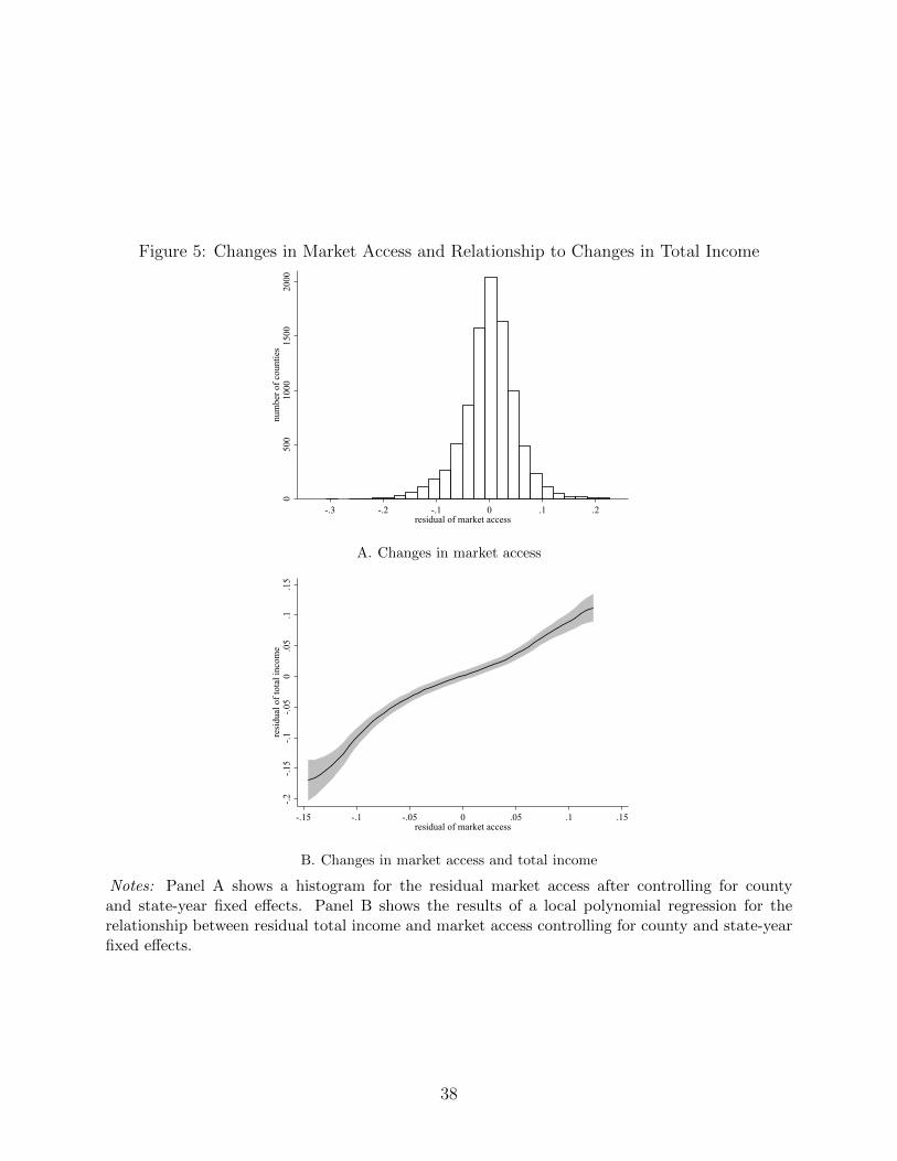
Figure 5: Changes in Market Access and Relationship to Changes in Total Income

050

010

0015

0020

00nu

mbe

r of c

ount

ies

-.3 -.2 -.1 0 .1 .2residual of market access

A. Changes in market access

-.2-.1

5-.1

-.05

0.0

5.1

.15

resi

dual

of t

otal

inco

me

-.15 -.1 -.05 0 .05 .1 .15residual of market access

B. Changes in market access and total income

Notes: Panel A shows a histogram for the residual market access after controlling for countyand state-year fixed effects. Panel B shows the results of a local polynomial regression for therelationship between residual total income and market access controlling for county and state-yearfixed effects.

38

Figure 6: Counterfactual Change in Market Access in Appalachian Counties without ADHS

Notes: The figure shows the difference between the actual change in market access between 19602010 and the counterfactual change in the absence of the ADHS. In each scenario, the change inmarket access is calculated between each county shown and all counties in the contiguous UnitedStates. Darker shades indicate counties that have relatively larger market access in the absence ofthe ADHS.

39

Figure 7: Convergence in Income Per Capita in ARC Relative to the Rest of the Country

-.3-.2

-.10

1960 1985 2010

ARC, actual w/ ADHS ARC, counteractual w/o ADHS

rela

tive

to U

S av

erag

e (in

per

cent

)

Notes: The figure shows the actual (solid line) and counterfactual (dashed line) income per capitain ARC counties relative to the rest of the country in 1985 and 2010. Counterfactual estimateswere constructed using the the change in the market access in 1985 and 2010 in the absence ofthe ADHS together with the estimated relationship between income per capita and market accessshown in column 3 of Table 3.

40

Table 1: Summary Statistics for Change in Market Access, Income, and Population

All US In states with counties in ARC:

Counties All ARC Non-ARC

(1) (2) (3) (4)

A. Change from 1960 to 1985

Income 1.08 1.19 1.14 1.22

[0.90] [0.36] [0.35] [0.36]

Population 0.18 0.20 0.19 0.20

[0.52] [0.27] [0.23] [0.30]

Income Per Capita 0.91 0.99 0.95 1.02

[0.34] [0.22] [0.21] [0.22]

Market Access 0.72 0.75 0.74 0.76

[0.13] [0.13] [0.12] [0.13]

B. Change from 1985 to 2010

Income 0.52 0.54 0.50 0.57

[0.77] [0.28] [0.27] [0.29]

Population 0.16 0.20 0.15 0.22

[0.46] [0.28] [0.28] [0.27]

Income Per Capita 0.35 0.35 0.35 0.34

[0.14] [0.12] [0.11] [0.13]

Market Access 0.13 0.13 0.11 0.14

[0.08] [0.06] [0.06] [0.06]

Sample Counties 3,080 1,070 397 673

Notes: The table shows summary statistics for the change in market access, total income, and totalpopulation from 1960 to 1985 and 1985 to 2010 for all sample counties (column 1) and stratifiedby whether counties were included in a state with at least one county in the Appalachian RegionalCommission program area (column 2), in the Appalachian Regional Commission (column 3), andnot in the Appalachian Regional Commission (column 4). Standard deviations are in parentheses.

41

Table 2: Results for Impact of Market Access on Total Income

A. Unweighted: B. Weighted: C. Local Controls:

OLS IV, 1st IV, 2nd OLS IV, 1st IV, 2nd OLS IV, 1st IV, 2nd

(1) (2) (3) (1) (2) (3) (1) (2) (3)

log(market access) 1.050 0.642 1.945 0.765 1.807 0.944

(0.214) (0.291) (0.228) (0.410) (0.204) (0.295)

log( travel time) -1.874 -1.486 -1.499

(0.096) (0.360) (0.287)

First Stage F -stat 381.18 16.99 27.35

Notes: The table shows the results from estimating equation (4). Panel A shows the unweighted results, Panel B shows the results ofweighting by income in 1960, and Panel C shows the results of weighting by income in 1960 and including local controls for distanceto IHS and ADHS, miles of IHS, ADHS, and other highways in 2010 interacted with year fixed effects. All panels include county andstate-year fixed effects as well as baseline controls for third-order polynomials in area (in square miles), latitude, longitude, and anindicator for whether the county is in a metropolitan statistical area, all interacted with year fixed effects. In each panel, column 1shows the results of using ordinary least squares, while columns 2 and 3 show the first- and second-stage results using instrumentalvariables. Standard errors (in parentheses) are clustered at the state level. The number of counties used is 3,080 and the total numberof observations is 9,240.

42

Table 3: Decomposition of Impact of Market Access on Total Income

Dependent variable is log of

Market Total Income Total

Access Income Per Capita Population

(1) (2) (3) (4)

log(market access) 0.944 0.429 0.552

(0.295) (0.144) (0.347)

log( travel time) -1.499

(0.287)

Notes: The table shows instrumental variables estimates of equation (4). Column 1 shows the first-stage result with log of market access as the dependent variable. Columns 2 through 4 show thesecond-stage results using log of total income, income per capita, and total population, respectively,as the dependent variable. Standard errors (in parentheses) are clustered at the state level. Thenumber of counties used is 3,080 and the total number of observations is 9,240.

Table 4: Results for Impact of Market Access on Total Income and the AppalachianRegional Commission

Dependent variable is log of

Market Market Total

Access Access × ARC Income

(1) (2) (3)

log(market access) 0.975

(0.310)

log(market access)×ARC -0.067

(0.088)

log( travel time) -1.507 0.054

(0.298) (0.040)

log( travel time)×ARC 0.020 -1.852

(0.043) (0.072)

Notes: The table shows instrumental variables estimates of equation (4) including an additionalinteraction term between log of market access and an indicator for whether a county is included inthe Appalachian Regional Commission. Columns 1 and 2 show the first-stage results with the log ofmarket access and the interaction term, respectively, as dependent variables. Column 3 shows thesecond-stage results with total income as the dependent variable. Standard errors (in parentheses)are clustered at the state level. The number of counties used is 3,080 and the total number ofobservations is 9,240.

43

Table 5: Results for Impact of Market Access on Employment by Sector

Employment Agriculture Construction Transportation Manufacturing Trade Finance Gov’t Other

(1) (2) (3) (4) (5) (6) (7) (8) (9)

log(market access) 1.273 -4.886 2.141 1.179 1.092 2.353 1.256 0.848 0.715

(0.554) (3.063) (1.038) (0.622) (0.452) (1.155) (0.709) (0.485) (0.463)

log(market access)×ARC -0.183 0.547 0.095 -0.298 -0.127 -0.341 -0.114 0.125 -0.181

(0.074) (0.489) (0.222) (0.130) (0.109) (0.123) (0.123) (0.111) (0.113)

Notes: The table shows the results of estimating a version equation (4) replacing log of total income as the outcome with log ofemployment by sector. In addition, the estimates for an interaction term between log of market access and an indicator for whethera county is included in the Appalachian Regional Commission are also shown. Column 1 shows the results for total employmentand columns 2 through 8 show the results for the sector given in the heading. In Column 6, “Other” includes the broad categoryof services, mining, and miscellaneous employment. Standard errors (in parentheses) are clustered at the state level. The number ofcounties used is 3,080 and the total number of observations is 9,240.

44

Table 6: Results for Impact of Market Access on Total Income by Year

Dependent variable is log of

Market Market Market Total

Access Access × 1985 Access × 2010 Income

(1) (2) (3) (4)

log(market access) 0.717

(0.538)

log(market access)× 1985 -0.067

(0.485)

log(market access)× 2010 0.420

(0.414)

log( travel time) -1.626 -0.194 -0.310

(0.393) (0.336) (0.329)

log( travel time)× 1985 0.391 -2.927 0.359

(0.257) (0.458) (0.233)

log( travel time)× 2010 0.123 0.280 -3.068

(0.297) (0.190) (0.518)

Notes: The table shows instrumental variables estimates of equation (4) including additionalinteraction terms between log of market access and indicators for whether year is 1985 or 2010.Columns 1 and 3 show the first-stage results with the log of market access and the interactionterms, respectively, as dependent variables. Column 4 shows the second-stage results with totalincome as the dependent variable. Standard errors (in parentheses) are clustered at the state level.The number of counties used is 3,080 and the total number of observations is 9,240.

45

Table 7: Counterfactual Impact of Market Access on Total Income

Market Access Counterfactual (in billions, 2015 $):

Coefficient w/o ADHS, 2010 w/o ADHS, 1985 w/ PARC, 2010

(1) (2) (3) (4)

Baseline Counterfactual 0.944 -33.4 -24.9 -13.9

(0.295) (9.8) (7.5) (4.1)

1. increase IHS speed 0.806 -22.9 -17.8 -10.7

(0.288) (7.9) (6.2) (3.7)

2. increase ADHS speed 0.953 -35.2 -24.7 -11.9

(0.328) (11.7) (8.3) (3.9)

3. fixed 1960 income 1.113 -39.0 -29.1 -16.3

(0.397) (13.0) (9.9) (5.4)

4. use population 1.019 -33.4 -24.9 -13.9

(0.326) (10.0) (7.6) (4.1)

5. set θ equal to 6 1.190 -33.4 -32.9 -13.7

(0.386) (10.3) (10.4) (4.2)

6. set θ equal to 10 0.811 -33.4 -20.9 -14.2

(0.246) (9.5) (6.0) (4.0)

7. exclude counties <250 miles 0.967 -34.2 -25.4 -14.3

(0.300) (10.0) (7.6) (4.1)

8. exclude counties <500 miles 0.941 -33.3 -24.8 -13.9

(0.315) (10.5) (8.0) (4.4)

Notes: The table shows the results and robustness for the impact of counterfactual changes inmarket access. Each row shows the estimated market access coefficient (column 1) as well as theresults under the two counterfactual scenarios for all sample counties (columns 2 and 3). Standarderrors (in parentheses) are clustered at the state level.

46

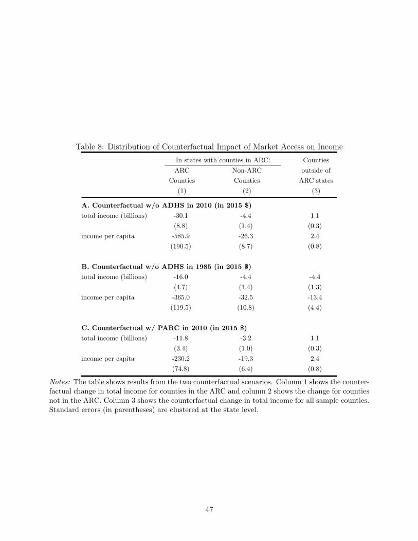
Table 8: Distribution of Counterfactual Impact of Market Access on Income

In states with counties in ARC: Counties

ARC Non-ARC outside of

Counties Counties ARC states

(1) (2) (3)

A. Counterfactual w/o ADHS in 2010 (in 2015 $)

total income (billions) -30.1 -4.4 1.1

(8.8) (1.4) (0.3)

income per capita -585.9 -26.3 2.4

(190.5) (8.7) (0.8)

B. Counterfactual w/o ADHS in 1985 (in 2015 $)

total income (billions) -16.0 -4.4 -4.4

(4.7) (1.4) (1.3)

income per capita -365.0 -32.5 -13.4

(119.5) (10.8) (4.4)

C. Counterfactual w/ PARC in 2010 (in 2015 $)

total income (billions) -11.8 -3.2 1.1

(3.4) (1.0) (0.3)

income per capita -230.2 -19.3 2.4

(74.8) (6.4) (0.8)

Notes: The table shows results from the two counterfactual scenarios. Column 1 shows the counter-factual change in total income for counties in the ARC and column 2 shows the change for countiesnot in the ARC. Column 3 shows the counterfactual change in total income for all sample counties.Standard errors (in parentheses) are clustered at the state level.

47

A Additional Figures & Tables

Table A1: Impact of Market Access on Total Income with Alternative Instruments

Dependent Variable

Total Market Total Market Total Market

Income Access Income Access Income Access

(1) (2) (3) (4) (5) (6)

log(market access) 0.944 0.967 0.941

(0.295) (0.300) (0.315)

log( travel time) -1.499 -1.505 -1.489

(0.287) (0.294) (0.325)

Instrument excludes counties: own state within 250 miles within 500 miles

First Stage F -stat 27.35 26.20 20.94

Notes: The tables shows results using alternative instruments when estimating equation (4).Columns 1 and 2 reproduce the first- and second-stage results using an instrument that excludesown-state counties when calculating the predicted travel time instrument. Columns 3 and 4 andcolumns 5 and 6 show first- and second-stage results using an instrument that excludes countieswithin 250 and 500 miles, respectively, when calculating the predicted travel time instrument. Stan-dard errors (in parentheses) are clustered at the state level. The number of counties used is 3,080and the total number of observations is 9,240.

48