1

NATIONAL OPEN UNIVERSITY OF NIGERIA

COURSE CODE : MTH 307

COURSE TITLE: NUMERICAL ANALYSIS II

2

Course Code: MTH 307:

Course Title: NUMERICAL ANALYSIS II

Course Developer/Writer: Dr. S. A. Okunuga Department of Mathematics, University of Lagos Akoka, Lagos, Nigeria

Course Editor: …

Programme Leader: …

Course Coordinator: …

NATIONAL OPEN UNIVERSITY OF NIGERIA

3

MTH 307: NUMERICAL ANALYSIS II 3 units Course content MODULE 1 APPROXIMATIONS Unit 1 Polynomials Unit 2 Least Squares Approximation (Discrete Case) Unit 3 Least Squares Approximation (Continuous Case) MODULE 2: ORTHOGONAL POLYNOMIALS Unit 1 Introduction to Orthogonal System Unit 2 The Legendre Polynomials Unit 3 Least Squares Approximations by Legendre Polynomials Unit 4 The Chebyshev Polynomials Unit 5 Series of Chebyshev Polynomials Unit 6 Chebyshev Approximations MODULE 3: FURTHER INTERPOLATION TECHNIQUES Unit 1 Cubic Splines Approximation Unit 2 Hermite Approximations MODULE 4 NUMERICAL INTEGRATION Unit 1 Introduction to Numerical Integration Unit 2 Trapezoidal Rule Unit 3 Simpson’s Rules Unit 4 Newton-Cotes Formulas MODULE 5: BOUNDARY VALUE PROBLEMS Unit 1 Introduction to BVP Unit 2 BVP involving Partial Differential Equation Unit 3 Solution of Laplace Equation in a Rectangle

4

MODULE 1

APPROXIMATIONS

UNIT 1: POLYNOMIALS 1.0 Introduction Polynomials are very useful in the study of Mathematics especially in Numerical Analysis. Over the years polynomials have been used as approximation to several functions. Although polynomials are sometimes difficult to solve as equations yet they help in appreciating the value of certain functions. To this end, polynomials are of paramount importance when it comes to approximation theory. 2.0 Objectives By the end of this unit, the learner should be able to:

(a) define a polynomial; (b) understand the degree of a polynomial; (c) distinguish between polynomial as a function and a polynomial equation; (d) express simple functions as polynomials (e) name types of approximation methods.

3.0 What is a Polynomial? From elementary Mathematics, you have come across polynomials in various forms. The commonest one is what is usually called the quadratic expression which can be written as

ax2 + bx + c Thus examples of polynomials may include: 2x2 – 3x +1

x2 + 6x – 5 x4 + 3x3- x 2 +2x + 5 and so on. We shall therefore give a standard definition of what a polynomial is Definition 1 A function P(x) of the form

P(x) = a0 + a

1x + a

2x

2 + … + a

nx

n (3.1)

is said to be a polynomial in x, where ao, a1, a2, . . . , an are the coefficients of the function P(x).

These coefficients may be real or complex numbers. 3.1 The Degree of a Polynomial

Definition 2

The highest power to which the variable x is raised in a polynomial P(x) is the degree of the polynomial. Hence, the polynomial function P(x) given by equation (3.1) is of degree n, For example any quadratic expression is a polynomial of degree 2.

5

If P(x) = x4 + 3x3- x 2 +2x + 5, then P(x) is of degree 4 2x2 – 3x +1 is a polynomial of degree two. 3.2 Polynomial Equation A polynomial is simply an expression whereas a polynomial can be come an equation if the expression is equated to a quantity, often to zero. Thus, when we write P(x) = 0 , from equation (3.1) then equation (3.1) becomes a polynomial equation. Although (3.1) is called an equation this is only because the polynomial is designated as P(x) on the left hand side. Apart from this, it is simply a polynomial. Thus a

0 + a

1x + a

2x

2 + … + a

nx

n

is a polynomial of degree n, whereas a

0 + a

1x + a

2x

2 + … + a

nx

n = 0 (3.2)

is a polynomial equation of degree n. We must observe that if all the terms of a polynomial exist, then the number of coefficients exceed the degree of the polynomial by one. Thus a polynomial of degree n given by equation (3.2) has n+1 coefficients. Polynomial equation can be solved to determine the value of the variable (say x) that satisfies the equation. On the other hand there is nothing to solve in a polynomial. At best you may factorize or expand a polynomial and never to solve for the value of the variable. Thus we can solve the polynomial equation 0223 =−+ xxx But we can only factorize xxx 223 −+ To factorize the expression xxx 223 −+ we shall get: x(x+2)(x – 1) But solving for x in the equation we get: x = –2 , 0, 1 There are many things that we can do with polynomials. One of such things is to use polynomials to approximate non-polynomial functions. 3.3 Function Approximation There are functions that are not polynomials but we may wish to represent such by a polynomial. For example, we may wish to write cos x or exp(x) in terms of polynomials. How do we achieve this? The learner should not confuse this with expansion of a seemly polynomial by Binomial expansion. For example, we can expand 8)1( x+ using binomial expansion. Without expanding this, the expression is simply a polynomial of degree 8. However, if we wish to write ex as a polynomial, then it can be written in the form:

......33

221 ++++++= n

nox xaxaxaxaae

This is only possible by using series expansion such as Taylor or Maclaurin series. The learner is assumed to have studied Taylor or Maclaurin series of simple functions at the lower level. For example, the expansion of exp(x) is written as:

...!

...!3!2

132

++++++=nxxxxe

nx

6

This shows that exp(x) can be expressed as a polynomial function. The degree of where the

polynomial is truncated (terminated), say !k

xk, is the approximation that is written for ex. It may

be reasonable to let k be large, say at least 2. Hence a fourth order approximation of exp(x) will be:

!4!3!21

432 xxxxex ++++= (3.3)

That is, ex is written here as a polynomial of degree 4. Similarly the Taylor series for cos x is given by

...!6!4!2

1cos642++++=

xxxx (3.4)

The illustration above leads us to the study of approximation theory. 3.4 Types of Functions Approximation

Before we go fully into the discussion of various approximations in Numerical Analysis, we need to state that there may arise two problems. The first problem arises when a function is given explicitly, but we wish to find a simpler type of function such as a polynomial, that can be used to approximate values of the given function. The second kind of problem in approximation theory is concerned with fitting functions to a given set of data and finding the “best” function in a certain class that can be used to represent the set of data. To handle these two problems, we shall in this study discuss some of the basic methods of approximations. Some of the approximation methods of functions, in existence, include:

(i.) Taylor’s Approximation (ii.) Lagrange polynomials (iii.) Least-Squares approximation (iv.) Hermite approximation (v.) Cubic Spline interpolation (vi.) Chebyshev approximation (vii.) Legendre Polynomials (viii.) Rational function approximation; and some few others more.

Every approximation theory involves polynomials; hence, some methods of approximation are sometimes called polynomials. For example, Chebyshev approximation is often referred to as Chebyshev polynomials. We shall begin this discussion of these approximations with the Least Squares Approximation. Self Assessment Exercise 1. How many non-zero coefficients has )1)(52( 2 −+ xx

2. What is the degree of the polynomial involved in the equation: 0)2)(12( 2 =−+x

xx ?

hence obtain its solution. 3. Write a polynomial of degree 3 with only two coefficients 4. By following equation (3.3) write down the expansion of e –x

7

4.0 Conclusion Polynomials are basic tools that can be used to express other functions in a simpler form. While it may be difficult to calculate e3 without a calculator, because the exponential function e is approximately 2.718, but we can simply substitute 3 into the expansion given by (3.3) and simplify to get an approximate value of e3. Hence a close attention should be given to this type of function. 5.0 Summary In this Unit we have learnt that (i) polynomials are expression involving various degrees of variable x which may be sum

together. (ii) polynomial expression is different from polynomial equation. (iii) simple functions can be written through the expansion given by Taylor or Maclaurin series. (iv) there are various polynomial approximations which can be used to estimate either a

function or a set of data. 6.0 Tutor Marked Assignment 1. Obtain the Taylor’s expansion of sin x 2. Distinguish between Taylor series and Binomial expansion 3. Find the Maclaurin series for e –x as far as the term involving x4 and hence estimate e –2 7.0 Further Reading and Other Resources.

1. Conte S. D. and Boor de Carl Elementary Numerical Analysis an Algorithmic Approach 2nd ed. McGraw-Hill Tokyo.

2. Francis Scheid. (1989) Schaum’s Outlines Numerical Analysis 2nd ed. McGraw-Hill New York.

3. Okunuga, S. A., and Akanbi M, A., (2004). Computational Mathematics, First Course, WIM Pub. Lagos, Nigeria.

4. Turner P. R. (1994) Numerical Analysis Macmillan College Work Out Series Malaysia

8

MODULE 1 UNIT 2: Least Squares Approximation (Discrete Case) 1.0 Introduction Sometimes we may be confronted with finding a function which may represent a set of data points which are given for both arguments x and y. Often it may be difficult to find such a function y = y(x) except by certain techniques. One of the known methods of fitting a polynomial function to this set of data is the Least squares approach. The least squares approach is a technique which is developed to reduce the sum of squares of errors in fitting the unknown function. The Least Squares Approximation methods can be classified into two, namely the discrete least square approximation and the continuous least squares approximation. The first involves fitting a polynomial function to a set of data points using the least squares approach, while the latter requires the use of orthogonal polynomials to determine an appropriate polynomial function that fits a given function. For these reasons, we shall treat them separately.

2.0 Objective By the end of this unit, you should be able to:

(a) handle fitting of polynomial (for discrete case) by least squares method (b) derive the least square formula for discrete data (c) fit a linear polynomial to a set of data points (d) fit a quadratic or parabolic polynomial to a set of data points

3.0 Discrete Least Squares Approximation The basic idea of least square approximation is to fit a polynomial function P(x) to a set of data points (xi, yi) having a theoretical solution

y = f(x) (3.1) The aim is to minimize the squares of the errors. In order to do this, suppose the set of data satisfying the theoretical solution ( 3.1) are

(x1, y1), (x2, y2), . . . , (xn, yn) Attempt will be made to fit a polynomial using these set of data points to approximate the theoretical solution f(x). The polynomial to be fitted to these set of points will be denoted by P(x) or sometimes Pn(x) to denote a polynomial of degree n. The curve or line P(x) fitted to the observation y1, y2, . . . , yn will be regarded as the best fit to f(x), if the difference between P(xi) and f(xi) , i = 1, 2, . . . , n is least. That is, the sum of the differences ei = f(xi) – P(xi), i = 1, 2, . . . , n should be the minimum. The differences obtained from ei could be negative or positive and when all these ei are summed up, the sum may add up to zero. This will not give the true error of the approximating polynomial. Thus to estimate the exact error sum, the square of these differences are more appropriate. In other words, we usually consider the sum of the squares of the deviations to get the best fitted curve. Thus the required equation for the sum of squares error is then written as

[ ]∑=

−=n

iii xPxfS

1

2)()( (3.2)

which will be minimized.

9

where P(x) is given by P(x) = a

0 + a

1x + a

2x

2 + … + a

nx

n (3.3)

The above approach can be viewed either in the discrete case or in the continuous case 3.1 Fitting of polynomials (Discrete case) We shall now derive the formula in discrete form that fits a set of data point by Least squares technique. The aim of least squares method is to minimize the error of squares. To do this we begin by substituting equations (3.1) and (3.3) in equation (3.2), this gives:

[ ]∑=

++++−=n

i

kikiioi xaxaxaayS

1

2221 )....( (3.4)

To minimize S, we must differentiate S with respect to ai and equate to zero. Hence, if we differentiate equation (3.4) partially with respect to a0, a1,…,ak, and equate each to zero, we shall obtain the following:

[ ] 0)....(21

221 =++++−−=

∂∂

∑=

n

i

kikiioi

oxaxaxaay

aS

[ ] 0)....(21

221

1=++++−−=

∂∂

∑=

in

i

kikiioi xxaxaxaay

aS

[ ] 0.)....(2 2

1

221

2=++++−−=

∂∂

∑=

in

i

kikiioi xxaxaxaay

aS (3.5)

………….

[ ] 0.)....(21

221 =++++−−=

∂∂

∑=

ki

n

i

kikiioi

kxxaxaxaay

aS

These can be written as

∑∑∑∑ ++++= kikiioi xaxaxanay ....2

21

∑∑∑∑∑ +++++= 132

21 .... k

ikiiioii xaxaxaxayx

∑∑∑∑∑ +++++= 242

31

22 .... kikiiioii xaxaxaxayx (3.6)

… . . . . . .

∑∑∑∑∑ ++++= ++ kik

ki

ki

kioi

ki xaxaxaxayx 22

21

1 ....

where ∑ is assumed as short form for ∑=

n

i 1

Solving equation (3.6) to determine a0, a1,…ak and substituting into equation (3.3) gives the best fitted curve to (3.1). The set of equations in (3.6) are called the Normal Equations of the Least Squares Method Equation (3.6) can only be used by creating a table of values corresponding to each sum and the sum is found for each summation. We shall now illustrate how to use the set of equations (3.6) in a tabular form. Self Assessment Exercise

1. For a quadratic approximation, how many columns will be required, list the variables for the columns excluding the given x and y columns.

2. Give one reason why we need to square the errors in a least square method.

10

3.2 Numerical Example Example 1

By using the Least Squares Approximation, fit (a) a straight line (b) a parabola

to the given data below

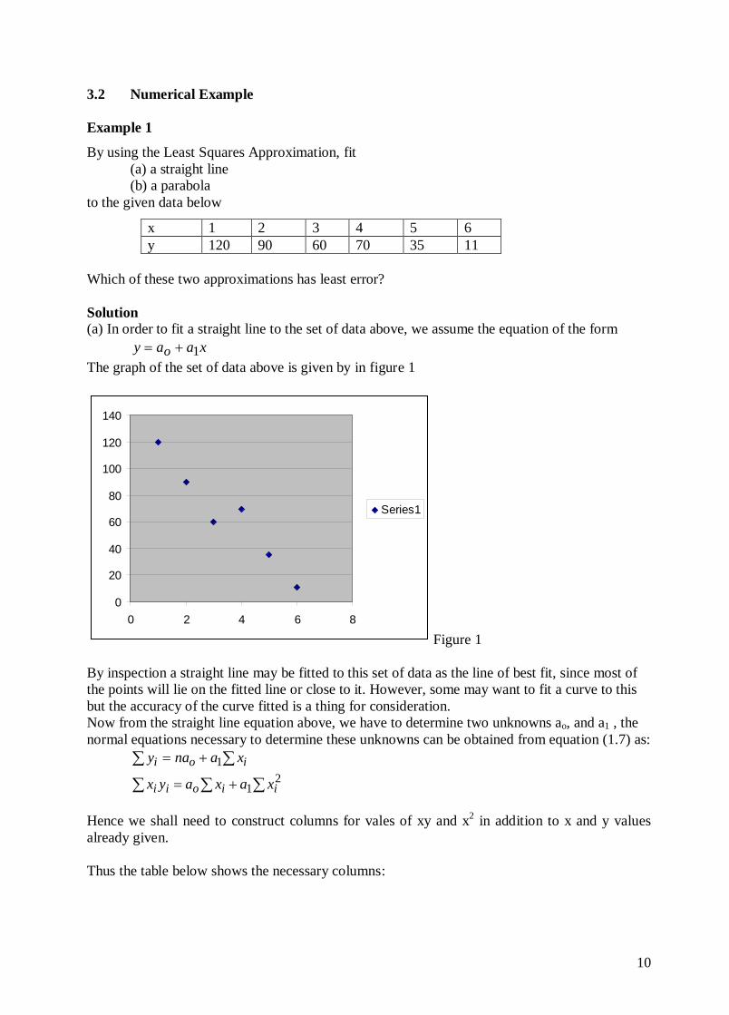
x 1 2 3 4 5 6 y 120 90 60 70 35 11

Which of these two approximations has least error? Solution (a) In order to fit a straight line to the set of data above, we assume the equation of the form xaay o 1+= The graph of the set of data above is given by in figure 1

0

20

40

60

80

100

120

140

0 2 4 6 8

Series1

Figure 1 By inspection a straight line may be fitted to this set of data as the line of best fit, since most of the points will lie on the fitted line or close to it. However, some may want to fit a curve to this but the accuracy of the curve fitted is a thing for consideration. Now from the straight line equation above, we have to determine two unknowns ao, and a1 , the normal equations necessary to determine these unknowns can be obtained from equation (1.7) as:

∑∑ += ioi xanay 1

∑∑∑ += 21 iioii xaxayx

Hence we shall need to construct columns for vales of xy and x2 in addition to x and y values already given. Thus the table below shows the necessary columns:

11

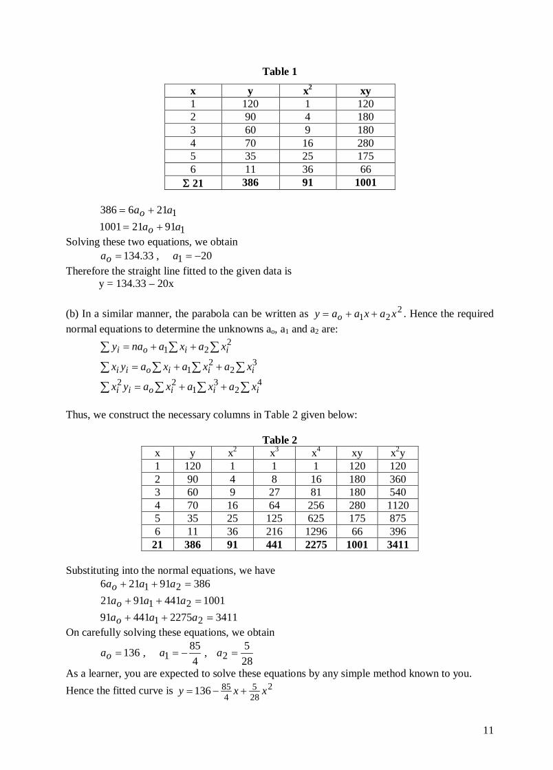
Table 1

x y x2 xy 1 120 1 120 2 90 4 180 3 60 9 180 4 70 16 280 5 35 25 175 6 11 36 66

Σ 21 386 91 1001

1

191211001

216386aa

aa

o

o+=

+=

Solving these two equations, we obtain 20,33.134 1 −== aao

Therefore the straight line fitted to the given data is y = 134.33 – 20x (b) In a similar manner, the parabola can be written as 2

21 xaxaay o ++= . Hence the required normal equations to determine the unknowns ao, a1 and a2 are:

∑∑∑ ++= 221 iioi xaxanay

∑∑∑∑ ++= 32

21 iiioii xaxaxayx

∑∑∑∑ ++= 42

31

22iiioii xaxaxayx

Thus, we construct the necessary columns in Table 2 given below:

Table 2 x y x2 x3 x4 xy x2y 1 120 1 1 1 120 120 2 90 4 8 16 180 360 3 60 9 27 81 180 540 4 70 16 64 256 280 1120 5 35 25 125 625 175 875 6 11 36 216 1296 66 396

21 386 91 441 2275 1001 3411 Substituting into the normal equations, we have

341122754419110014419121

38691216

21

21

21

=++=++

=++

aaaaaa

aaa

o

o

o

On carefully solving these equations, we obtain

285,

485,136 21 =−== aaao

As a learner, you are expected to solve these equations by any simple method known to you. Hence the fitted curve is 2

285

485136 xxy +−=

12

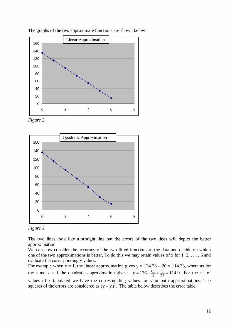
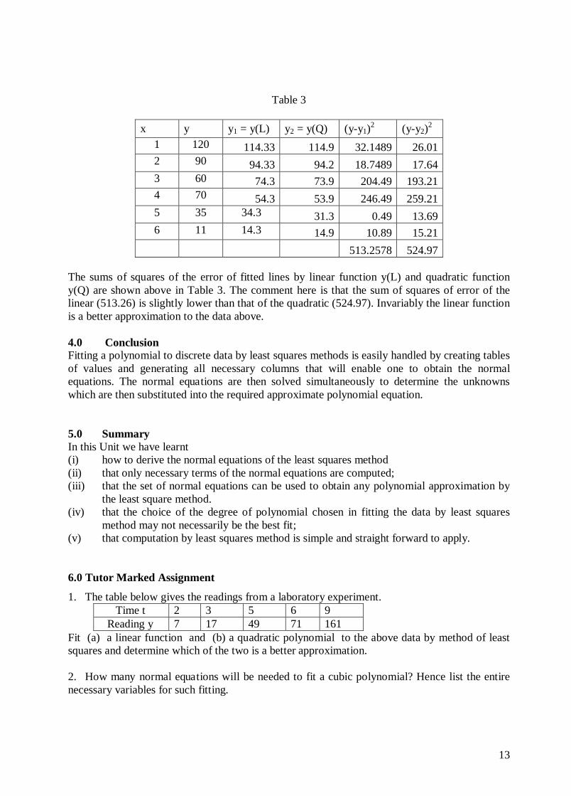
The graphs of the two approximate functions are shown below:

0

20

40

60

80

100

120

140

160

0 2 4 6 8

Figure 2

0

20

40

60

80

100

120

140

160

0 2 4 6 8

Figure 3 The two lines look like a straight line but the errors of the two lines will depict the better approximation. We can now consider the accuracy of the two fitted functions to the data and decide on which one of the two approximations is better. To do this we may retain values of x for 1, 2, . . . , 6 and evaluate the corresponding y values. For example when x = 1, the linear approximation gives y = 134.33 – 20 = 114.33, where as for the same x = 1 the quadratic approximation gives: 9.114136 28

54

85 =+−=y . For the set of

values of x tabulated we have the corresponding values for y in both approximations. The squares of the errors are considered as (y – yi)2. The table below describes the error table.

Quadratic Approximation

Linear Approximation

13

Table 3

x y y1 = y(L) y2 = y(Q) (y-y1)2 (y-y2)2 1 120 114.33 114.9 32.1489 26.01 2 90 94.33 94.2 18.7489 17.64 3 60 74.3 73.9 204.49 193.21 4 70 54.3 53.9 246.49 259.21 5 35 34.3 31.3 0.49 13.69 6 11 14.3 14.9 10.89 15.21

513.2578 524.97 The sums of squares of the error of fitted lines by linear function y(L) and quadratic function y(Q) are shown above in Table 3. The comment here is that the sum of squares of error of the linear (513.26) is slightly lower than that of the quadratic (524.97). Invariably the linear function is a better approximation to the data above. 4.0 Conclusion Fitting a polynomial to discrete data by least squares methods is easily handled by creating tables of values and generating all necessary columns that will enable one to obtain the normal equations. The normal equations are then solved simultaneously to determine the unknowns which are then substituted into the required approximate polynomial equation. 5.0 Summary In this Unit we have learnt (i) how to derive the normal equations of the least squares method (ii) that only necessary terms of the normal equations are computed; (iii) that the set of normal equations can be used to obtain any polynomial approximation by

the least square method. (iv) that the choice of the degree of polynomial chosen in fitting the data by least squares

method may not necessarily be the best fit; (v) that computation by least squares method is simple and straight forward to apply. 6.0 Tutor Marked Assignment

1. The table below gives the readings from a laboratory experiment. Time t 2 3 5 6 9

Reading y 7 17 49 71 161 Fit (a) a linear function and (b) a quadratic polynomial to the above data by method of least squares and determine which of the two is a better approximation. 2. How many normal equations will be needed to fit a cubic polynomial? Hence list the entire necessary variables for such fitting.

14

7.0 Further Reading and Other Resources 1. Conte S. D. and Boor de Carl Elementary Numerical Analysis an Algorithmic Approach

2nd ed. McGraw-Hill Tokyo. 2. Francis Scheid. (1989) Schaum’s Outlines Numerical Analysis 2nd ed. McGraw-Hill New

York. 3. Okunuga, S. A., and Akanbi M, A., (2004). Computational Mathematics, First Course,

WIM Pub. Lagos, Nigeria. 4. Turner P. R. (1994) Numerical Analysis Macmillan College Work Out Series Malaysia 5. Atkinson K.E. (1978): An Introduction to Numerical Analysis, 2nd Edition, John Wiley &

Sons, N.Y

15

MODULE 1 UNIT 3 Least Squares Approximation (Continuous Case) 1.0 Introduction We have seen in the last unit how to fit a polynomial to a set of data points by using the least squares approximation technique. We shall in this unit consider the situation in which a function f(x) is to be approximated by the least squares method in terms of a polynomial. In this case since data are no longer given, it would not be necessary to create tables by columns but rather by carrying out some integration. The candidate is therefore required to be able to integrate simple functions as may be required. 2.0 Objective By the end of this unit, the learner should be able to

(i.) Distinguish between discrete data and continuous function (ii.) Fit polynomials to continuous functions by least squares approach

3.0 Fitting an Approximate Polynomials (Continuous case) If we wish to find a least square approximation to a continuous function f(x), our previous approach must be modified since the number of points (xi, yi) at which the approximation is to be measured is now infinite (and non-countable). Therefore, we cannot use a summation as

[ ]∑=

−n

iii xPxf

1

2)()( , but we must use a continuous measure, that is an integral. Hence if the

interval of the approximation is [a, b], so that bxa ≤≤ for all points under consideration, then we must minimize

[ ]∫ −ba

dxxPxf 2)()(

where y = f(x) is our continuous function and P(x) is our approximating function. 3.1 Derivation Let f(x) be a continuous function which in the interval (a, b) is to be approximated by a polynomial linear combination

kko xaxaxaaxP ++++= ....)( 2

21 (3.1)

[ ] dxxaxaxaaySba

kikiioi∫ ++++−=

2221 )....(

of n+1 given functions no ϕϕϕϕ ,...,, 21 . Then, c0, c1, …, cn can be determined such that a weighted Euclidean norm of the error function f(x) – p(x) becomes as small as possible

That is, ∫ −=−b

adxxwxPxfxPxf )()()()()( 22 (3.2)

where w(x) is a non-negative weighting function. Equation (3.2) is the continuous least square approximation problem. The minimization problem of f(x) by continuous function P(x) of( 3.1) is given by

[ ]∫ −=ba

dxxPxfS 2)()( (3.3)

where the interval [a, b] is usually normalized to [-1,1] following Legendre polynomial or Chebyshev function approximation, hence, substituting equation (3.2) in (3.3), we obtain

16

[ ]∫− ++++−=1

12

2211 )()}(...)()()({)( dxxwxcxcxcxcxfS nnoo ϕϕϕϕ (3.4)

where no ϕϕϕϕ ,...,, 21 are some chosen polynomials. To minimize (3.3) or (3.4), one could consider two alternative methods to obtain the coefficients or the unknown terms. 3.1.1 First Method The first approach for minimizing equation (3.3) is by carrying out an expansion of the term [ ]2)()( xPxf − , next carry out the integration and then by means of calculus, obtain the minimum by setting

0=∂∂

kcS , k = 0, 1, 2, …, n

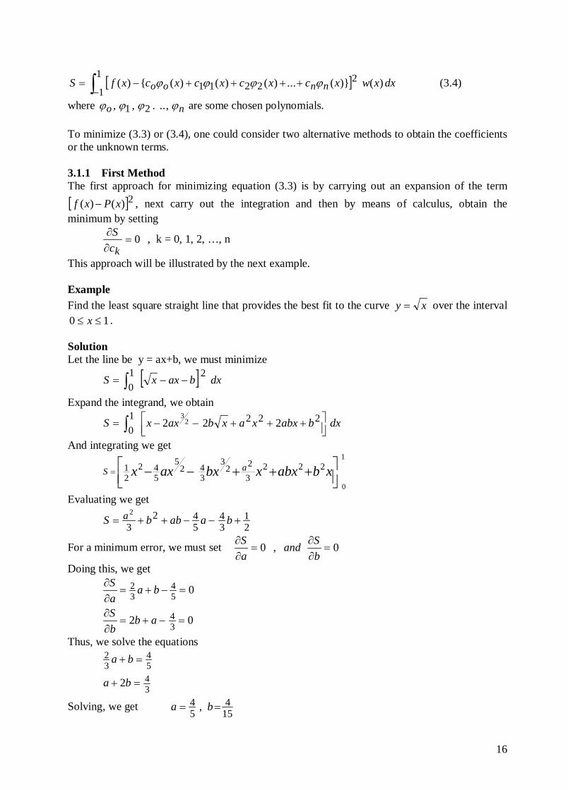
This approach will be illustrated by the next example. Example Find the least square straight line that provides the best fit to the curve xy = over the interval

10 ≤≤ x . Solution Let the line be y = ax+b, we must minimize

[ ]∫ −−=10

2 dxbaxxS

Expand the integrand, we obtain

∫

+++−−=

10

222 222 23

dxbabxxaxbaxxS

And integrating we get

+++−−= xbabxxbxaxx aS 222

322

3

342

5

542

21

1

0

Evaluating we get

21

34

542

32

+−−++= baabbS a

For a minimum error, we must set 0,0 =∂∂

=∂∂

bSand

aS

Doing this, we get

02

0

34

54

32

=−+=∂∂

=−+=∂∂

abbS

baaS

Thus, we solve the equations

3454

32

2 =+

=+

ba

ba

Solving, we get 154

54 , == ba

17

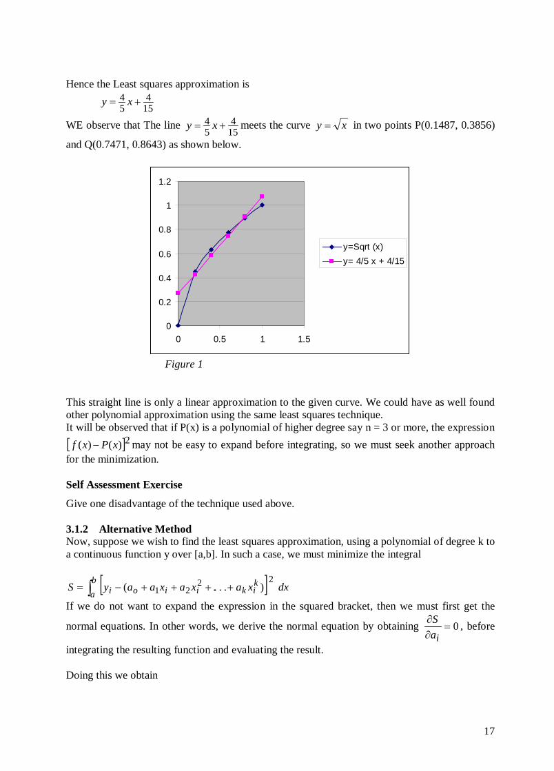
Hence the Least squares approximation is

154

54 += xy

WE observe that The line 154

54 += xy meets the curve xy = in two points P(0.1487, 0.3856)

and Q(0.7471, 0.8643) as shown below.

0

0.2

0.4

0.6

0.8

1

1.2

0 0.5 1 1.5

y=Sqrt (x)y= 4/5 x + 4/15

Figure 1

This straight line is only a linear approximation to the given curve. We could have as well found other polynomial approximation using the same least squares technique. It will be observed that if P(x) is a polynomial of higher degree say n = 3 or more, the expression [ ]2)()( xPxf − may not be easy to expand before integrating, so we must seek another approach for the minimization. Self Assessment Exercise

Give one disadvantage of the technique used above. 3.1.2 Alternative Method Now, suppose we wish to find the least squares approximation, using a polynomial of degree k to a continuous function y over [a,b]. In such a case, we must minimize the integral

[ ] dxxaxaxaaySba

kikiioi∫ ++++−=

2221 )....(

If we do not want to expand the expression in the squared bracket, then we must first get the

normal equations. In other words, we derive the normal equation by obtaining 0=∂∂

iaS , before

integrating the resulting function and evaluating the result. Doing this we obtain

18

( ) 0....2 221 =−−−−−−=

∂∂

∫ dxxaxaxaayaS b

ak

koio

( ) 0....2 221

1=−−−−−−=

∂∂

∫ dxxaxaxaayxaS b

ak

koi

( ) 0....2 221

2

2=−−−−−−=

∂∂

∫ dxxaxaxaayxaS b

ak

koi

and in general we can write

0....2 221 =

−−−−−−=

∂∂

∫ dxxaxaxaayxaS b

ak

koir

r for (r = 0,1, . . . , k )

The factor (–2) that appeared first in the integral can be ignored since the right hand side of the equation is zero. Hence, the normal equations can be written as

0....221 =

−−−−−∫ dxxaxaxaayx

ba

kkoi

r for (r = 0,1, . . . , k )

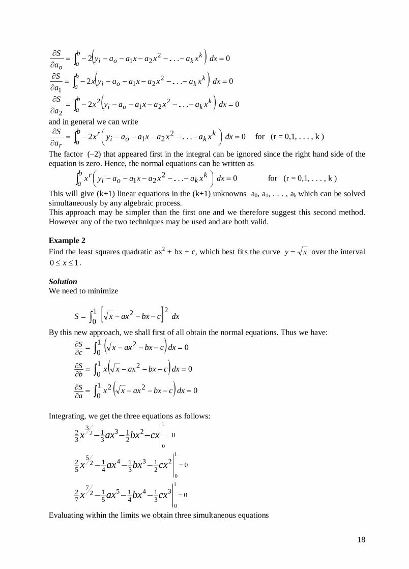
This will give (k+1) linear equations in the (k+1) unknowns a0, a1, . . . , ak which can be solved simultaneously by any algebraic process. This approach may be simpler than the first one and we therefore suggest this second method. However any of the two techniques may be used and are both valid. Example 2 Find the least squares quadratic ax2 + bx + c, which best fits the curve xy = over the interval

10 ≤≤ x . Solution We need to minimize

[ ]∫ −−−=10

22 dxcbxaxxS

By this new approach, we shall first of all obtain the normal equations. Thus we have:

( ) 010

2 =−−−= ∫∂∂ dxcbxaxxcS

( ) 010

2 =−−−= ∫∂∂ dxcbxaxxxbS

( ) 010

22 =−−−= ∫∂∂ dxcbxaxxxaS

Integrating, we get the three equations as follows:

02213

312

3

32

1

0

=−−− cxbxaxx

02213

314

412

5

52

1

0

=−−− cxbxaxx

03314

415

512

7

72

1

0

=−−− cxbxaxx

Evaluating within the limits we obtain three simultaneous equations

19

72

31

41

51

52

21

31

41

32

21

31

=++

=++

=++

cba

cba

cba

Solving these equations simultaneously we get

356,

3548,

74

==−= cba

Thus the least squares quadratic function is

356

3548

74)( 2 ++−= xxxf

or ( )32410352)( 2 −−−= xxxf

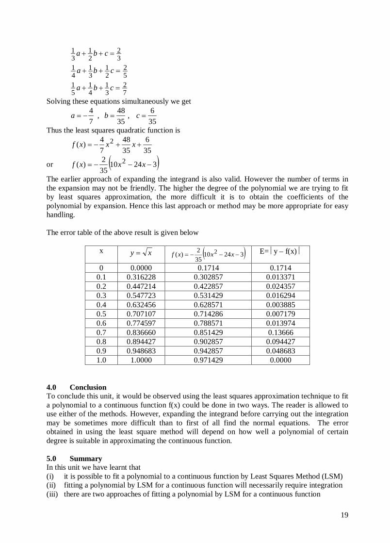
The earlier approach of expanding the integrand is also valid. However the number of terms in the expansion may not be friendly. The higher the degree of the polynomial we are trying to fit by least squares approximation, the more difficult it is to obtain the coefficients of the polynomial by expansion. Hence this last approach or method may be more appropriate for easy handling. The error table of the above result is given below

x xy = ( )32410352)( 2 −−−= xxxf E= y – f(x)

0 0.0000 0.1714 0.1714 0.1 0.316228 0.302857 0.013371 0.2 0.447214 0.422857 0.024357 0.3 0.547723 0.531429 0.016294 0.4 0.632456 0.628571 0.003885 0.5 0.707107 0.714286 0.007179 0.6 0.774597 0.788571 0.013974 0.7 0.836660 0.851429 0.13666 0.8 0.894427 0.902857 0.094427 0.9 0.948683 0.942857 0.048683 1.0 1.0000 0.971429 0.0000

4.0 Conclusion To conclude this unit, it would be observed using the least squares approximation technique to fit a polynomial to a continuous function f(x) could be done in two ways. The reader is allowed to use either of the methods. However, expanding the integrand before carrying out the integration may be sometimes more difficult than to first of all find the normal equations. The error obtained in using the least square method will depend on how well a polynomial of certain degree is suitable in approximating the continuous function. 5.0 Summary In this unit we have learnt that (i) it is possible to fit a polynomial to a continuous function by Least Squares Method (LSM) (ii) fitting a polynomial by LSM for a continuous function will necessarily require integration (iii) there are two approaches of fitting a polynomial by LSM for a continuous function

20

(iv) one approach will require expansion of [f(x) – P(x)]2 for a given polynomial P(x) while the other approach will go by the way of normal equation.

6.0 Tutor Marked Assignment Find the least squares quadratic ax2 + bx + c, which best fits the curve 12 += xy over the interval 10 ≤≤ x . 7.0 Further Reading and Other Resources

1. Francis Scheid. (1989) Schaum’s Outlines Numerical Analysis 2nd ed. McGraw-Hill New York.

2. Turner P. R. (1994) Numerical Analysis Macmillan College Work Out Series Malaysia 3. Atkinson K.E. (1978): An Introduction to Numerical Analysis, 2nd Edition, John Wiley &

Sons, N.Y 4. Leadermann Walter (1981) (Ed.): Handbook of Applicable Mathematics, Vol 3,

Numerical Analysis, John Wiley, N.Y.

21

MODULE 2

ORTHOGONAL POLYNOMIALS

UNIT 1 Introduction To Orthogonal System 1.0 Introduction Orthogonal polynomials are of fundamental importance in many branches of mathematics in addition to approximation theory and their applications are numerous but we shall be mainly concerned with two special cases, the Legendre polynomials and the Chebyshev polynomials. More general applications are however easily worked out once the general principles have been understood. 2.0 Objective By the end of this unit, the learner should be able to

(i.) define what orthogonal polynomials are (ii.) formulate orthogonal and orthonormal polynomials (iii.) handle inner product of functions

3.0 Orthogonal Polynomials We begin this study by giving the definition of orthogonal functions: Definition 1 A system of real functions ....),(),( 1 xxo φφ defined in an interval [a,b] is said to be orthogonal in this interval if

=≠

=∫ nmnm

dxxxn

ba nm ,

,0)()(

λφφ

If 1.....10 === λλ the system is said to be normal. An orthogonal system which is also normal is sometimes referred to as an orthonormal system. Note that since )(xnφ is real, λn ≥ 0 and we shall assume that each )(xnφ is continuous and non-zero so that λn > 0. The advantages offered by the use of orthogonal functions in approximation theory can now be made clear as follows. Suppose {φn,(x)} is an orthogonal system and that f(x) is any function and we wish to express f(x) in the form ....)(....)()()( 11 ++++= xcxcxcxf nnoo φφφ (3.1)

Then nnb

ann

b

an cdxxcdxxxf λφφ == ∫∫ )()()( 2

since all the other terms on the right-hand side are zero and so

dxxxfcb

ann

n ∫= )()(1 φλ

(3.2)

Thus the coefficients cn in equation (3.1) can be found. These coefficients cn are called the Fourier coefficients of f(x), with respect to the system {φn(x)} 3.1 The Inner Products Let w(x) be the weighting function and let the inner product of two continuous functions f(x) and g(x) be defined as

22

∫=ba

dxxgxfxwgf )()()(,

where f, g are continuous in [a, b], then f(x) and g(x) satisfy the following properties: (i.) ,,,, ><=><=>< gfgfgf ααα α is a scalar (ii.) gfgfgff ,,, 2121 +=+

(iii.) 2121 ,,, gfgfggf +=+

(iv.) fggf ,, =

(v) 0, >ff for all f ∈ C[a,b] and 0, =ff iff f = 0. The functions f and g are said to be orthogonal if the inner product of f and g is zero, that is if

0, =gf In a similar manner we can define the inner product for the discrete case. The inner product of discrete functions f and g satisfy the orthogonality property given by

∑=

=m

kkk xgxfgf

0)()(,

where {xk} are the zeroes of the function. We remark here that polynomial approximation is one of the best ways to fit solution to unknown function f(x). A good polynomial Pn(x) which is an approximation to a continuous function f(x) in a finite range [a, b] must possess oscillatory property. Among such polynomial approximation functions include the Chebyshev Polynomials and the Legendre Polynomials. We shall examine these polynomials and their properties in our discussion in this course as we go along. Definition 2 (Orthogonality with respect to a weight function) A series of functions {φn,(x)} are said to be orthogonal with respect to the weight function w(x) over (a,b) if

=≠

=∫ nmnm

dxxwxxn

ba nm ,

,0)()()(

λφφ

The idea and principle of orthogonality properties are now extended to two common polynomials in the next few sections. 3.2 EXAMPLE The best-known example of an orthogonal system is the trigonometric system

1, cos x, sin x, cos2x, sin2x,…

Over the interval [-π, π]. We shall define various combination of integral of product functions of sine and cosine as follows:

)(0sincos

)(0coscos

nmdxmxnx

nmdxmxnx

≠=

≠=

∫

∫

−

−ππ

ππ

23

)(0sinsin

)(0cossin

nmdxmxnx

nmdxmxnx

≠=

≠=

∫

∫

−

−ππ

ππ

and )0(0sin.cos ≠==∫− nmdxnxnxππ

whereas )(0coscos nmdxnxnx ==∫−ππ

⇒ dxnxdxnx ∫∫ −−+=

ππ

ππ

)2cos1(cos 212

πππππ

π

π

=−+−−+=

+=−

))(2sin()2sin(

)2sin(

21

21

21

21

21

21

nn

nxx

nn

n

Also )(0sinsin nmdxnxnx ==∫−ππ

⇒ )0(sin 2 ≠==∫− nmdxnx πππ

and finally for n = 0, )0(210cos 22 ==== ∫∫ −−nmdxdx π

ππ

ππ

Comparing this with our Definition 1 above, we obtain from these integrals the following values

πλλπλ ==== ...,2 321 It follows therefore that the system

πππππ

xxxx 2sin,2cos,sin,cos,21

is orthogonal and normal 4.0 Conclusion The discussion above has simply illustrates the way to determine where a set of functions is orthogonal or otherwise. Other examples can be produced to show the orthogonality property. 5.0 Summary In this unit we have learnt that

(i.) a normal orthogonal system is an orthonormal system (ii.) orthogonality of some functions can be obtained by integration (iii.) inner product is written as an integral or a sum

6.0 Tutor Marked Assignment Verify whether the following functions are orthogonal or not (i.) 1, ex , e2x , e3x , . . . . (ii.) ln x, ln2x , ln3x , ln4x, . . . 7.0 Further Reading and Other Resources

1. Francis Scheid. (1989) Schaum’s Outlines Numerical Analysis 2nd ed. McGraw-Hill New York.

24

2. Turner P. R. (1994) Numerical Analysis Macmillan College Work Out Series Malaysia 3. Atkinson K.E. (1978): An Introduction to Numerical Analysis, 2nd Edition, John Wiley &

Sons, N.Y 4. Leadermann Walter (1981) (Ed.): Handbook of Applicable Mathematics, Vol 3,

Numerical Analysis, John Wiley, N.Y.

25

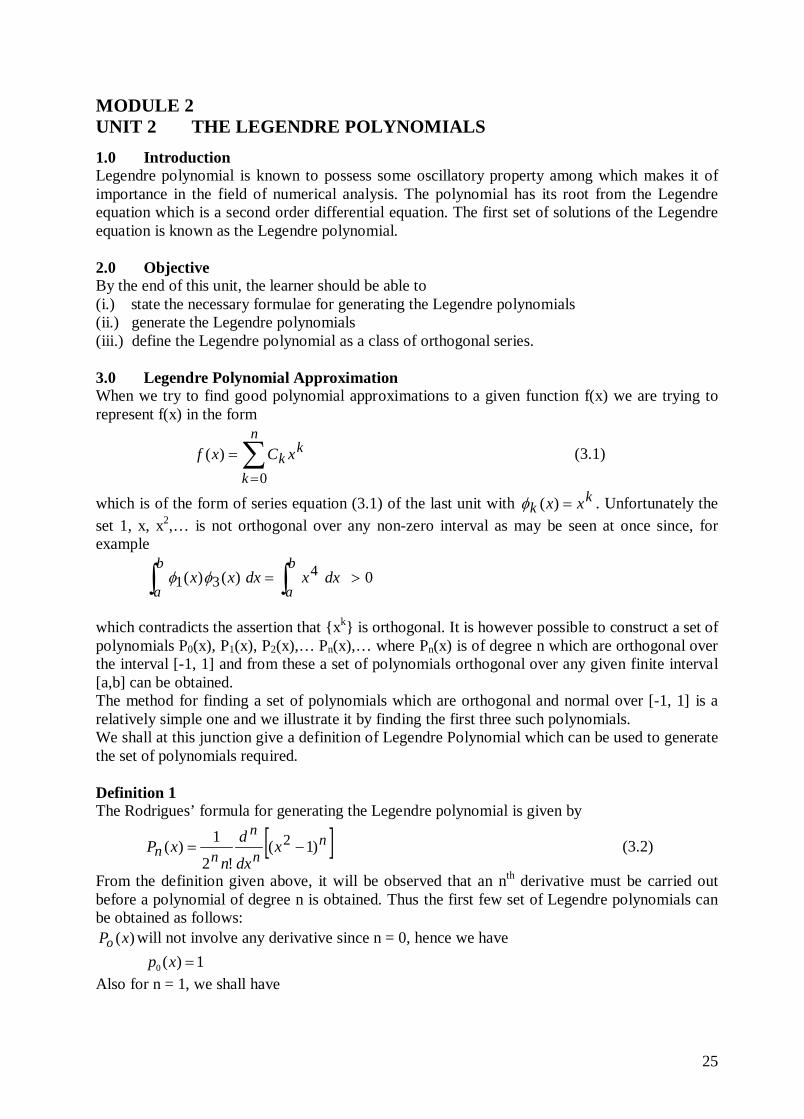
MODULE 2 UNIT 2 THE LEGENDRE POLYNOMIALS 1.0 Introduction Legendre polynomial is known to possess some oscillatory property among which makes it of importance in the field of numerical analysis. The polynomial has its root from the Legendre equation which is a second order differential equation. The first set of solutions of the Legendre equation is known as the Legendre polynomial. 2.0 Objective By the end of this unit, the learner should be able to (i.) state the necessary formulae for generating the Legendre polynomials (ii.) generate the Legendre polynomials (iii.) define the Legendre polynomial as a class of orthogonal series. 3.0 Legendre Polynomial Approximation When we try to find good polynomial approximations to a given function f(x) we are trying to represent f(x) in the form

∑=

=n

k

kk xCxf

0)( (3.1)

which is of the form of series equation (3.1) of the last unit with kk xx =)(φ . Unfortunately the

set 1, x, x2,… is not orthogonal over any non-zero interval as may be seen at once since, for example

0)()( 431 >= ∫∫ dxxdxxx

b

a

b

aφφ

which contradicts the assertion that {xk} is orthogonal. It is however possible to construct a set of polynomials P0(x), P1(x), P2(x),… Pn(x),… where Pn(x) is of degree n which are orthogonal over the interval [-1, 1] and from these a set of polynomials orthogonal over any given finite interval [a,b] can be obtained. The method for finding a set of polynomials which are orthogonal and normal over [-1, 1] is a relatively simple one and we illustrate it by finding the first three such polynomials. We shall at this junction give a definition of Legendre Polynomial which can be used to generate the set of polynomials required. Definition 1 The Rodrigues’ formula for generating the Legendre polynomial is given by

[ ]nn

n

nn xdx

d

nxP )1(

!2

1)( 2 −= (3.2)

From the definition given above, it will be observed that an nth derivative must be carried out before a polynomial of degree n is obtained. Thus the first few set of Legendre polynomials can be obtained as follows:

)(xPo will not involve any derivative since n = 0, hence we have

0 ( ) 1p x = Also for n = 1, we shall have

26

xxxdxdxP ==−= 2.)1(.

!1.21)( 2

1211

[ ]222

2

22 )1(!22

1)( −= xdxdxP

)44(81)12(

81)( 324

2

22 xx

dxdxx

dxdxP −=+−=

)13(21)412(

81)( 22

2 −=−= xxxP

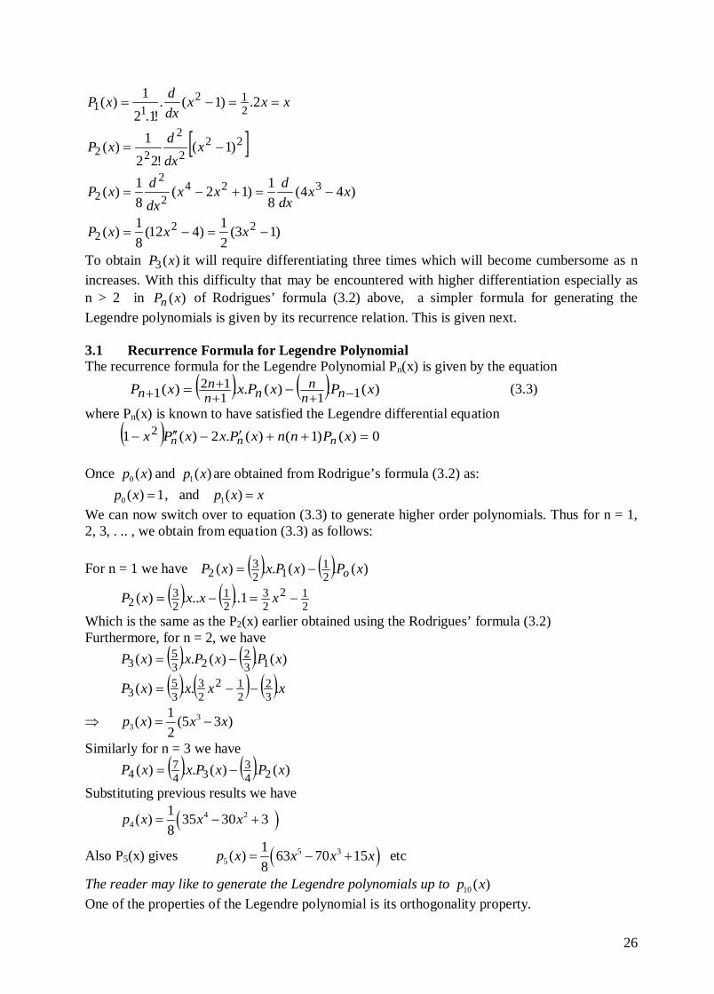
To obtain )(3 xP it will require differentiating three times which will become cumbersome as n increases. With this difficulty that may be encountered with higher differentiation especially as n > 2 in )(xPn of Rodrigues’ formula (3.2) above, a simpler formula for generating the Legendre polynomials is given by its recurrence relation. This is given next. 3.1 Recurrence Formula for Legendre Polynomial The recurrence formula for the Legendre Polynomial Pn(x) is given by the equation

( ) ( ) )(.)(..)( 11112

1 xPxPxxP nnn

nnn

n −+++

+ −= (3.3)

where Pn(x) is known to have satisfied the Legendre differential equation ( ) 0)()1()(.2)(1 2 =++′−′′− xPnnxPxxPx nnn Once 0 ( )p x and 1( )p x are obtained from Rodrigue’s formula (3.2) as: 0 ( ) 1p x = , and 1( )p x x= We can now switch over to equation (3.3) to generate higher order polynomials. Thus for n = 1, 2, 3, . .. , we obtain from equation (3.3) as follows: For n = 1 we have ( ) ( ) )(.)(..)( 2

112

32 xPxPxxP o−=

( ) ( )212

23

21

23

2 1.....)( −=−= xxxxP

Which is the same as the P2(x) earlier obtained using the Rodrigues’ formula (3.2) Furthermore, for n = 2, we have ( ) ( ) )(.)(..)( 13

223

53 xPxPxxP −=

( ) ( ) ( )xxxxP ...)( 32

212

23

35

3 −−=

⇒ 33

1( ) (5 3 )2

p x x x= −

Similarly for n = 3 we have ( ) ( ) )(.)(..)( 24

334

74 xPxPxxP −=

Substituting previous results we have

( )4 24

1( ) 35 30 38

p x x x= − +

Also P5(x) gives ( )5 35

1( ) 63 70 158

p x x x x= − + etc

The reader may like to generate the Legendre polynomials up to 10 ( )p x One of the properties of the Legendre polynomial is its orthogonality property.

27

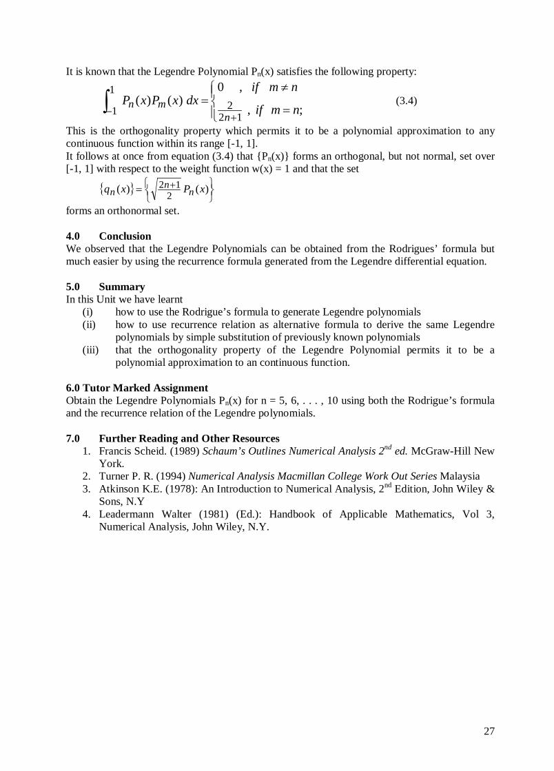
It is known that the Legendre Polynomial Pn(x) satisfies the following property:

=

≠=

+−∫ ;,

,0)()(

122

1

1 nmif

nmifdxxPxP

nmn (3.4)

This is the orthogonality property which permits it to be a polynomial approximation to any continuous function within its range [-1, 1]. It follows at once from equation (3.4) that {Pn(x)} forms an orthogonal, but not normal, set over [-1, 1] with respect to the weight function w(x) = 1 and that the set

{ }

= + )()(

212 xPxq n

nn

forms an orthonormal set. 4.0 Conclusion We observed that the Legendre Polynomials can be obtained from the Rodrigues’ formula but much easier by using the recurrence formula generated from the Legendre differential equation. 5.0 Summary In this Unit we have learnt

(i) how to use the Rodrigue’s formula to generate Legendre polynomials (ii) how to use recurrence relation as alternative formula to derive the same Legendre

polynomials by simple substitution of previously known polynomials (iii) that the orthogonality property of the Legendre Polynomial permits it to be a

polynomial approximation to an continuous function. 6.0 Tutor Marked Assignment Obtain the Legendre Polynomials Pn(x) for n = 5, 6, . . . , 10 using both the Rodrigue’s formula and the recurrence relation of the Legendre polynomials. 7.0 Further Reading and Other Resources

1. Francis Scheid. (1989) Schaum’s Outlines Numerical Analysis 2nd ed. McGraw-Hill New York.

2. Turner P. R. (1994) Numerical Analysis Macmillan College Work Out Series Malaysia 3. Atkinson K.E. (1978): An Introduction to Numerical Analysis, 2nd Edition, John Wiley &

Sons, N.Y 4. Leadermann Walter (1981) (Ed.): Handbook of Applicable Mathematics, Vol 3,

Numerical Analysis, John Wiley, N.Y.

28

MODULE 2 UNIT 3 Least Squares Approximation by Legendre Polynomials 1.0 Introduction Legendre Polynomials are known to be applicable to least square approximation of functions. In this sense, we mean that we can follow the least square approximation technique and adapt this to Legendre polynomial. 2.0 Objective By the end of this unit, the learner should be able to

(i.) apply Legendre polynomial to least squares procedures (ii.) obtain least square approximation using Legendre polynomial

3.0 The Procedure

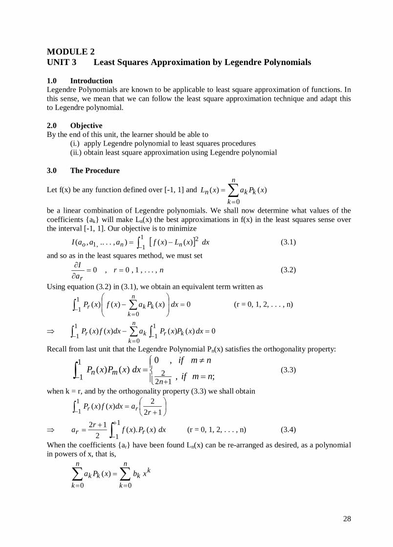
Let f(x) be any function defined over [-1, 1] and ∑=

=n

kkkn xPaxL

0)()(

be a linear combination of Legendre polynomials. We shall now determine what values of the coefficients {ak} will make Ln(x) the best approximations in f(x) in the least squares sense over the interval [-1, 1]. Our objective is to minimize

[ ]∫− −=11

2,1 )()(),....,( dxxLxfaaaI nno (3.1)

and so as in the least squares method, we must set

nraI

r,...,1,0,0 ==

∂∂ (3.2)

Using equation (3.2) in (3.1), we obtain an equivalent term written as

0)()()(0

11

=

− ∑∫

=−

dxxPaxfxPn

kkkr (r = 0, 1, 2, . . . , n)

⇒ 0)()()()(11

0

11

=− ∫∑∫ −=

−dxxPxPadxxfxP kr

n

kkr

Recall from last unit that the Legendre Polynomial Pn(x) satisfies the orthogonality property:

=

≠=

+−∫ ;,

,0)()(

122

1

1 nmif

nmifdxxPxP

nmn (3.3)

when k = r, and by the orthogonality property (3.3) we shall obtain

+=∫− 12

2)()(11 r

adxxfxP rr

⇒ dxxPxfra rr ∫+

−

+=

1

1)().(

212 (r = 0, 1, 2, . . . , n) (3.4)

When the coefficients {ar} have been found Ln(x) can be re-arranged as desired, as a polynomial in powers of x, that is,

∑∑==

=n

k

kk

n

kkk xbxPa

00)(

29

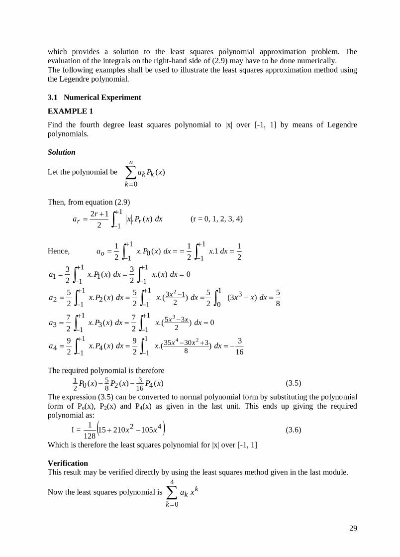
which provides a solution to the least squares polynomial approximation problem. The evaluation of the integrals on the right-hand side of (2.9) may have to be done numerically. The following examples shall be used to illustrate the least squares approximation method using the Legendre polynomial. 3.1 Numerical Experiment

EXAMPLE 1

Find the fourth degree least squares polynomial to |x| over [-1, 1] by means of Legendre polynomials. Solution

Let the polynomial be ∑=

n

kkk xPa

0)(

Then, from equation (2.9)

dxxPxra rr ∫+

−

+=

1

1)(.

212 (r = 0, 1, 2, 3, 4)

Hence, 211.

21)(.

21 1

1

1

10 ==== ∫∫

+

−

+

−dxxdxxPxao

0)(.23)(.

23 1

1

1

111 === ∫∫

+

−

+

−dxxxdxxPxa

85)3(

25)(.

25)(.

25 1

031

1 2131

122

2=−=== ∫∫∫

+

−−+

−dxxxdxxdxxPxa x

0)(.27)(.

27 1

1 2351

133

3=== ∫∫

+

−−+

−dxxdxxPxa xx

163)(.

29)(.

29 1

1 8330351

144

24−=== ∫∫ −

+−+

−dxxdxxPxa xx

The required polynomial is therefore )()()( 416

328

502

1 xPxPxP −− (3.5)

The expression (3.5) can be converted to normal polynomial form by substituting the polynomial form of Po(x), P2(x) and P4(x) as given in the last unit. This ends up giving the required polynomial as:

I = ( )42 10521015128

1 xx −+ (3.6)

Which is therefore the least squares polynomial for |x| over [-1, 1] Verification This result may be verified directly by using the least squares method given in the last module.

Now the least squares polynomial is ∑=

4

0k

kk xa

30

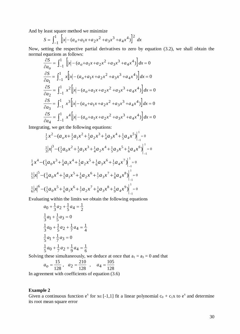
And by least square method we minimize

[ ]∫ − ++++−=11

244

33

221 )( dxxaxaxaxaaxS o

Now, setting the respective partial derivatives to zero by equation (3.2), we shall obtain the normal equations as follows:

[ ] 0)(11

44

33

221 =++++−=

∂∂

∫ − dxxaxaxaxaaxaS

oo

[ ] 0)(11

44

33

221

1=++++−=

∂∂

∫ − dxxaxaxaxaaxxaS

o

[ ] 0)(11

44

33

221

2

2=++++−=

∂∂

∫ − dxxaxaxaxaaxxaS

o

[ ] 0)(11

44

33

221

3

3=++++−=

∂∂

∫ − dxxaxaxaxaaxxaS

o

[ ] 0)(11

44

33

221

4

4=++++−=

∂∂

∫ − dxxaxaxaxaaxxaS

o

Integrating, we get the following equations:

0545

1434

1323

1212

1221 )(

1

1=++++−

−xaxaxaxaxax o

0646

1535

1424

1313

1202

1331 )(

1

1=++++−

−xaxaxaxaxax

0747

1636

1525

1414

1303

1441 )(

1

1=++++−

−xaxaxaxaxax

0848

1737

1626

1515

1404

1551 )(

1

1=++++−

−xaxaxaxaxax

0949

1838

1727

1616

1505

1661 )(

1

1=++++−

−xaxaxaxaxax

Evaluating within the limits we obtain the following equations

21

451

231

0 =++ aaa

0351

131 =+ aa

41

471

251

031 =++ aaa

0371

151 =+ aa

61

491

271

051 =++ aaa

Solving these simultaneously, we deduce at once that a1 = a3 = 0 and that

128105,

128210,

12815

42 === aaao

In agreement with coefficients of equation (3.6) Example 2 Given a continuous function ex for x∈[-1,1] fit a linear polynomial c0 + c1x to ex and determine its root mean square error

31

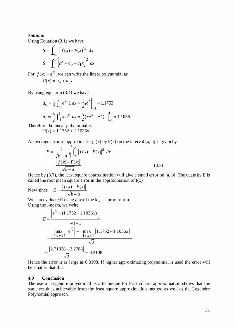
Solution Using Equation (3.1) we have

[ ]∫− −=1

12)()( dxxPxfS

[ ]∫− −−=1

1

21 dxxcceS o

x

For xexf =)( , we can write the linear polynomial as xaaxP o 1)( +=

By using equation (3.4) we have

1752.1211.

1

1

112

1 ===−−∫

xdxea exo

1036.1)(.23 1

1231

11 =−==−−∫

xxx exedxexa

Therefore the linear polynomial is P(x) = 1.1752 + 1.1036x

An average error of approximating f(x) by P(x) on the interval [a, b] is given by

∫ −−

=b

adxxPxf

abE 2)()(1

ab

xPxf−

−=

)()( (3.7)

Hence by (3.7), the least square approximation will give a small error on [a, b]. The quantity E is called the root mean square error in the approximation of f(x)

Now since ab

xPxfE

−

−=

)()(

We can evaluate E using any of the k-, l- , or m- norm Using the l-norm, we write

11

)1036.11752.1(

+

+−= l

x xeE

2

1036.11752.1maxmax1111

xex

xx

+−

=<<−<<−

3108.02

2788.271828.2=

−=

Hence the error is as large as 0.3108. If higher approximating polynomial is used the error will be smaller that this. 4.0 Conclusion The use of Legendre polynomial as a technique for least square approximation shows that the same result is achievable from the least square approximation method as well as the Legendre Polynomial approach.

32

5.0 Summary In this Unit the reader have learnt (i.) the technique of using Legendre polynomial to obtain and approximation using the least

square method. (ii.) that both Legendre approach and the Least squares approach will often produce the same

result. 6.0 Tutor Marked Assignment Obtain a fourth degree least squares polynomial for

xxf 1)( = over [-1, 1] by means of Legendre

polynomials. 7.0 Further Reading and Other Resources

1. Abramowitz M., Stegun I. (eds) ,(1964): Handbook of Mathematical functions, Dover , N.Y.

2. Conte S. D. and Boor de Carl Elementary Numerical Analysis an Algorithmic Approach 2nd ed. McGraw-Hill Tokyo.

3. Francis Scheid. (1989) Schaum’s Outlines Numerical Analysis 2nd ed. McGraw-Hill New York.

4. Henrici P. (1982): Essential of Numerical Analysis, Wiley, N.Y 5. Kandassamy P., Thilagarathy K., & Gunevathi K. (1997) : Numerical Methods, S. Chand

& Co Ltd, New Delhi, India

33

MODULE 2 UNIT 4: The Chebyshev Polynomials 1.0 Introduction It is always possible to approximate a continuous function with arbitrary precision by a polynomial of sufficient high degree. One of such approach is by using the Taylor series method. However, the Taylor series approximation of a continuous function f is often not so accurate in the approximation of f over an interval [ ba, ]. If the approximation is to be uniformly accurate over the entire interval. This may be due to the fact that: (i) in some cases, the Taylor series may either converge too slowly or not at all. (ii) the function may not be analytic or if it is analytic the radius of convergence of the Taylor series may be too small to cover comfortably the desired interval. In addition, the accuracy of the Taylor series depends greatly on the number of terms contained in the series. However, a process that was based on the fundamental property of Chebyshev polynomial may be considered as alternative and it works uniformly over any given interval. We know that there are several special functions used for different purposes including approximation, polynomial fittings and solutions of differential equations. Some of these special functions include Gamma, Beta, Chebyshev, Hermite, Legendre, Laguerre and so on. However, not all these are good polynomial approximation to continuous functions. However, Chebyshev polynomials have been proved to be very useful in providing good approximation to any continuous function. To this end, the Chebyshev polynomial is usually preferable as polynomial approximation. The Chebyshev polynomial has equal error property and it oscillates between –1 and 1. Due to its symmetric property, a shifted form of the polynomial to half the range (0, 1) is also possible. 2.0 Objective

By the end of this unit, the learner should be able to (i.) state the necessary formulae for generating the Chebyshev polynomials (ii.) obtain Chebyshev polynomials Tn(x) up to n = 10 (iii.) classify Chebyshev polynomial as a family of orthogonal series.

3.0 Introduction To Chebyshev Polynomials

As it was earlier stated, Chebyshev polynomials are often useful in approximating some functions. For this reason we shall examine the nature, properties and efficiency of the Chebyshev polynomial. Chebyshev Polynomial is based on the function “cos nθ” which is a polynomial of degree n in cosθ. Thus we give the following basic definition of the Chebyshev polynomial. Definition 1 The Chebyshev polynomial is defined in terms of cosine function as

)cos.cos()( 1 xnxTn−= for 0,11 ≥≤≤− nx (3.1)

This definition can be translated to polynomials of x as it would be discussed very soon. Before we do this, if we put x = cosθ , the Chebyshev polynomial defined above becomes

)cos()( θnxTn = Tn(x) is of the orthogonal family of polynomials of degree n and it has a weighting function

34

11,1

1)(2

≤≤−−

= xx

xw

It has an oscillatory property that in πθ ≤≤0 the function has alternating equal maximum and minimum values of ± 1 at the n+1 points

nr

rπθ = , r = 0, 1, 2, . . . , n.

or

=

nrxrπcos , r = 0, 1, 2, . . . , n

Thus the orthogonality relation of the Chebyshev polynomial is given as:

≠=

==≠

=∫− −0,

0,,0

)().(

21

1

1 11

2

mn

mnmn

dxxTxT mnx

π

π (3.2)

It also has a symmetric property given by )()1()( xTxT n

nn −=− (3.3)

3.1 Generating Chebyshev Polynomials Over the years the function Tn(x) is the best polynomial approximation function known for f(x). In order to express Tn(x) in terms of polynomials the definition can be used to some extent, but as n value increases, it becomes more difficult to obtain the actual polynomial except by some trigonometric identities, techniques and skill. For the reason, a simpler way of generating the Chebyshev polynomials is by using the recurrence formula for Tn(x) in [-1, 1]. The recurrence formula for generating the Chebyshev polynomial Tn(x) in [-1, 1] is given by

1,)()(2)( 11 ≥−= −+ nxTxxTxT nnn (3.4) Thus to obtain the Chebyshev polynomials, a combination of (3.1) and (3.4) can be used. Starting with the definition (3.1), that is

)cos.cos()( 1 xnxTn−=

We obtain the least polynomial when n = 0 as 10cos)(0 ==xT

Also when n = 1, we get xxxT == − )cos(cos)( 11

When n = 2, )cos2cos()( 12 xxT −=

with x = cosθ

12

1cos2

2cos)(

2

22

−=

−=

=

x

xT

θ

θ

For n = 3, 4, . . . it will be getting more difficult to obtain the polynomials. However if we use the recurrence formula (3.4) , we can obtain T2(x) by putting n = 1 so that

)()(2)( 012 xTxxTxT −= Substituting xxTxT == )(,1)( 10 , (from the result earlier obtained), we have

121).(2)( 22 −=−= xxxxT

35

This is simpler than using the trigonometric identity. Thus for n = 2, 3, . . . we obtain the next few polynomials as follows: When n = 2, the recurrence formula gives

xx

xxx

xTxxTxT

34

)12(2

)()(2)(

3

2123

−=

−−=

−=

Similarly for n = 3, we obtain

188

)12()34(2

)()(2)(

24

23234

+−=

−−−=

−=

xx

xxxx

xTxxTxT

In a similar manner xxxxT 52016)( 35

5 +−= We can now write all these polynomials out for us to see the pattern which they form.

xxTxT==

)(1)(

1

0

12)( 22 −= xxT

xxxT 34)( 33 −= (3.5)

188)( 244 +−= xxxT

xxxxT 52016)( 355 +−=

You can now derive the next few ones, say up to T10(x), following the same technique. Note that the recurrence formula is one step higher than the definition for the “n” value being used. In other words, when n = 2 in the definition we obtain T2(x), whereas to get the same T2(x) from the recurrence formula we use n = 1. The reason is obvious; the recurrence formula starts with subscript “n+1” as against “n” in the definition. These polynomials are of great importance in approximation theory and in solving differential equations by numerical techniques. 3.2 Properties of Chebyshev Polynomials In the interval –1 ≤ x ≤ 1 the Chebyshev Polynomial Tn(x) satisfies the following properties:

(i.) – 1 ≤ Tn(x) ≤ +1

(ii.) Tn(x) = 1 at (n + 1) points x0, x1, . . . , xn, where

=

nrxrπcos , r = 0, 1, 2, . . . , n

(iii.) nn xT )1()( −=

(iv.) The leading coefficient in Tn(x) is 2n – 1 . 3.3 Derivation of the Recurrence Formula

Now that we have seen the usefulness of the recurrence formula (2.16), it might be necessary for us to derive this formula from certain definition. There are two ways to this. We can use some trigonometric functions to get this since Chebyshev polynomial is defined as a cosine function. However, we can also derive this formula by solving it as a difference equation which can be shown to produce the definition (2.13). For the purpose of this course, since we are not treating linear difference equation, we shall go via the first type, by using some trigonometric functions.

36

Equation (2.16) is given by 1,)()(2)( 11 ≥−= −+ nxTxxTxT nnn

To obtain this formula, we can recall from trigonometric knowledge that )(cos)(cos2coscos

21

21 BABABA −+=+

If we put A = (n + 1) arccos x and B = (n – 1) arccos x Then cos A + cos B = cos{(n + 1)arccos x} + cos{(n – 1)arccos x} = [ ] [ ]xnnxnn arccos)11(cos.arccos)11(cos2 2

121 +−+−++

= [ ] ( )xxn arccos2cos.arccos)2(cos2 21

21

= 2 cos(n.arccos x) . cos(arccos x) cos A + cos B = 2cos(n arccos x). x cos A = 2xcos(n arccos x) – cos B That is cos[(n + 1)arccos x] = 2x cos[n arccos x] – cos[(n – 1)arccos x] By definition, )cos.cos()( 1 xnxTn

−= , we then have )()(2)( 11 xTxxTxT nnn −+ −= Thus the recurrence formula is easily established. 4.0 Conclusion The derivation of Chebyshev polynomials has been demonstrated and made simple by using the recurrence formula rather than using the basic definition (3.1). we have equally given the derivation of the recurrence formula by simply using some trigonometry identities, although this derivation can be established by solving the recurrence formula as a difference equation from which the basic definition (3.1) is obtained. Other methods of derivation equally exist. 5.0 Summary In this Unit we have learnt that: (i) Chebyshev polynomials are special kind of polynomials that satisfy some properties (ii) Chebyshev polynomials which are valid within [-1, 1] have either odd indices or even

indices for Tn(x) depending on whether n is odd or even. (iii) Chebyshev polynomials can be obtained from the recurrence formula. (iv) the recurrence formula for Chebyshev polynomials Tn(x) is more suitable to generate the

polynomials than its definition. 6.0 Tutor Marked Assignment Obtain the Chebyshev polynomials Tn(x) for n = 5, 6, . . . , 10 7.0 Further Reading and Other Resources 1. Abramowitz M., Stegun I. (eds), (1964): Handbook of Mathematical functions, Dover, N.Y. 2. Atkinson K.E. (1978): An Introduction to Numerical Analysis, 2nd Edition, John Wiley & Sons, N.Y 3. Conte S. D. and Boor de Carl Elementary Numerical Analysis an Algorithmic Approach 2nd ed.

McGraw-Hill Tokyo. 4. Henrici P. (1982): Essential of Numerical Analysis, Wiley, N.Y 5. Kandassamy P., Thilagarathy K., & Gunevathi K. (1997) : Numerical Methods, S. Chand & Co Ltd,

New Delhi, India 6. Leadermann Walter (1981) (Ed.): Handbook of Applicable Mathematics, Vol 3, Numerical Analysis,

John Wiley, N.Y. 7. Turner P. R. (1994) Numerical Analysis Macmillan College Work Out Series Malaysia

37

MODULE 2 UNIT 5: Series of Chebyshev Polynomials 1.0 Introduction Chebyshev polynomials can be used to make some polynomial approximations as against the use of least square method. The orthogonality properties of the Chebyshev polynomial permit the use of the polynomial as approximation to some functions. A case of cubic approximation will be considered in this study. 2.0 Objective By the end of this unit the learner would have learn (i) the form of the function f(x) which permits the use of Chebyshev polynomials as

approximation to it (ii) how to apply Chebyshev polynomials to fit a cubic approximation to a function f(x). 3.0 Approximation By Chebyshev Polynomials If we have a function f(x) which we wish to approximate with a series of Chebyshev polynomials

)(....)()()( 221121 xTcxTcxTccxf nno ++++= (3.1)

How we can find the coefficients ci?

The theoretical method is to multiply f(x) by 21

)(

x

xTm

− and integrate over [-1, 1], thereby making

use of the orthogonality property of Tn(x). Thus, if we multiply both sides by this factor and integrate over [-1, 1], we can write

∑ ∫∫∫=

−−− −+

−=

−

n

m

mnm

mo

m dxx

xTxTcdx

x

xTcdx

x

xTxf

1

11 2

11 22

111 2 1

)()(

1

)(

1

)()(

The only term on the right which doesn’t vanish is the one where m = n ≠ 0. In other words if we use the orthogonality property given by equation (3.2) of the last unit, we have

mm cdxx

xTxfπ2

111 21

)()(=

−∫−

dxx

xTxfc m

m ∫− −=

11 2

2

1

)()(π

(3.2)

The evaluation of the integral for cm given by (3.2) will in general have to be done numerically and in such cases it is obviously important to ensure that the truncation error is sufficiently small or the accuracy available via the Chebyshev approximation to f(x) will be reduced. In a few special cases, the integral can be evaluated analytically and the problem of truncation error does not arise; the most important of such case is when f(x) = xn (n ≥ 0) and we shall deal with this case below; but first we look at an example where evaluation of (3.2) is computed numerically. 3.1 Numerical Examples Example 1 Find a cubic approximation to ex by using Chebyshev polynomials Solution Let the approximation be

)(....)()( 221121 xTcxTcxTcce nno

x ++++=

38

Then, from (2.17)

dxx

xTec rx

r ∫− −=

1

1 22

1

)(π

(r = 0, 1, 2, 3)

Using the substitution x = cosθ , we transform this integral as follows:

x = cosθ ⇒ θθθθθ dxdddx 22 1cos1sin −−=−−=−= when x = 1 , θ = 0 and when x = - 1, θ = π Substituting into the integral above, we have

θθπ

θ

πdx

x

recr

−−

−= ∫ 20

2

cos2 1

1

)cos(

Canceling out the common terms and reversing the limits which eliminates the (-) sign we obtain

θθπ θ

πdrecr ∫=

0cos2 )cos( (3.3)

This is better from a numerical point of view since the integrand no longer contains a singularity. In evaluating integrals containing a periodic function as a factor in the integrand it is usually best to make use of the simplest quadrature formulae, such as the midpoint rule, Simpson rule or trapezium rule. By using any of these methods the coefficients cj can be evaluated for a series of decreasing step-sizes and the results compared. This will established some confidence in the accuracy of the results. Thus using the trapezoidal (or simply trapezium) rule with step-sizes π/2k (k=1,2,3,4) )2.....22()( 1212 nno

h yyyyyxf +++++= −

where h is the step size. From equation (3.3), we obtain the following estimates for c0

θπ θ

πdeco ∫=

0cos2

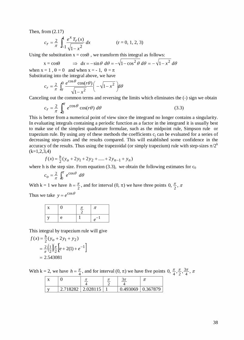
With k = 1 we have 2π=h , and for interval (0, π) we have three points ππ ,,0 2

Thus we take θcosey =

x 0 2π π

y e 1 1−e This integral by trapezium rule will give

( )( )[ ]543081.2

)1(2

)2()(

122

12

212

=

++=

++=

−ee

yyyxf oh

ππ

With k = 2, we have

4π=h , and for interval (0, π) we have five points ππππ ,,,,0 4

324

x 0 4π

2π

43π π

y 2.718282 2.028115 1 0.493069 0.367879

39

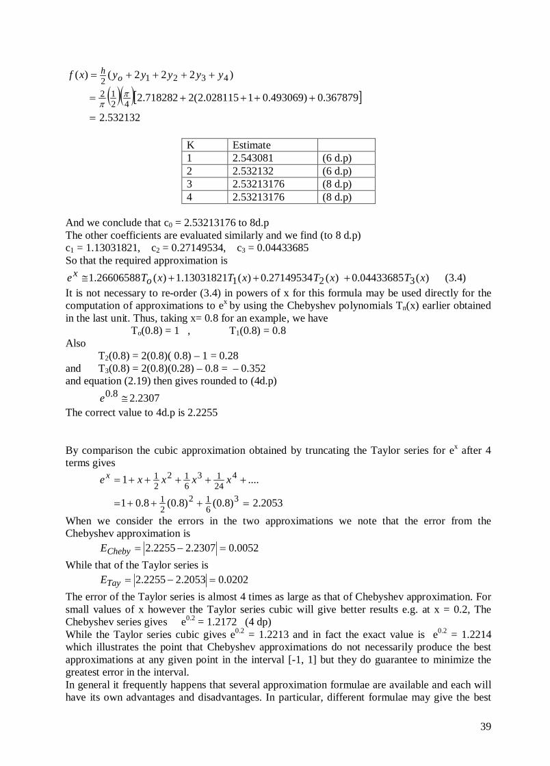
( )( )[ ]532132.2

367879.0)493069.01028115.2(2718282.2

)222()(

4212

43212

=

++++=

++++=

ππ

yyyyyxf oh

K Estimate 1 2.543081 (6 d.p) 2 2.532132 (6 d.p) 3 2.53213176 (8 d.p) 4 2.53213176 (8 d.p)

And we conclude that c0 = 2.53213176 to 8d.p The other coefficients are evaluated similarly and we find (to 8 d.p) c1 = 1.13031821, c2 = 0.27149534, c3 = 0.04433685 So that the required approximation is

)(04433685.0)(27149534.0)(13031821.1)(26606588.1 321 xTxTxTxTe ox +++≅ (3.4)

It is not necessary to re-order (3.4) in powers of x for this formula may be used directly for the computation of approximations to ex by using the Chebyshev polynomials Tn(x) earlier obtained in the last unit. Thus, taking x= 0.8 for an example, we have To(0.8) = 1 , T1(0.8) = 0.8 Also T2(0.8) = 2(0.8)( 0.8) – 1 = 0.28 and T3(0.8) = 2(0.8)(0.28) – 0.8 = – 0.352 and equation (2.19) then gives rounded to (4d.p) 2307.28.0 ≅e The correct value to 4d.p is 2.2255 By comparison the cubic approximation obtained by truncating the Taylor series for ex after 4 terms gives

2053.2)8.0()8.0(8.01

....1

3612

21

42413

612

21

=+++=

+++++= xxxxex

When we consider the errors in the two approximations we note that the error from the Chebyshev approximation is 0052.02307.22255.2 =−=ChebyE While that of the Taylor series is 0202.02053.22255.2 =−=TayE The error of the Taylor series is almost 4 times as large as that of Chebyshev approximation. For small values of x however the Taylor series cubic will give better results e.g. at x = 0.2, The Chebyshev series gives e0.2 = 1.2172 (4 dp) While the Taylor series cubic gives e0.2 = 1.2213 and in fact the exact value is e0.2 = 1.2214 which illustrates the point that Chebyshev approximations do not necessarily produce the best approximations at any given point in the interval [-1, 1] but they do guarantee to minimize the greatest error in the interval. In general it frequently happens that several approximation formulae are available and each will have its own advantages and disadvantages. In particular, different formulae may give the best

40

results over different parts of the interval of approximation and it may require considerable analysis to decide which to use at any point. We now consider the special case when f(x) = xn (n ≥ 0). The importance of this case lies in its role in the method of economization. It is possible to express the Chebyshev the term xn , n = 1, 2, 3, . . . in terms of Tn(x). These Chebyshev representations for xn are easily obtained by solving the Chebyshev polynomials successively as follows: T0(x) = 1 hence x0 = 1 = T0(x) T1(x) = x hence x = T1(x) T2(x) = 2x2 – 1 = 2x2 – T0(x) , hence x2 = ½ [T2(x) + T0(x)] T3(x) = 4x3 –3x = 4x3 – 3T1(x) , hence x3 = ¼ [T3(x) + 3T0(x)] Similarly, ( ))(3)(4)( 0248

14 xTxTxTx ++=

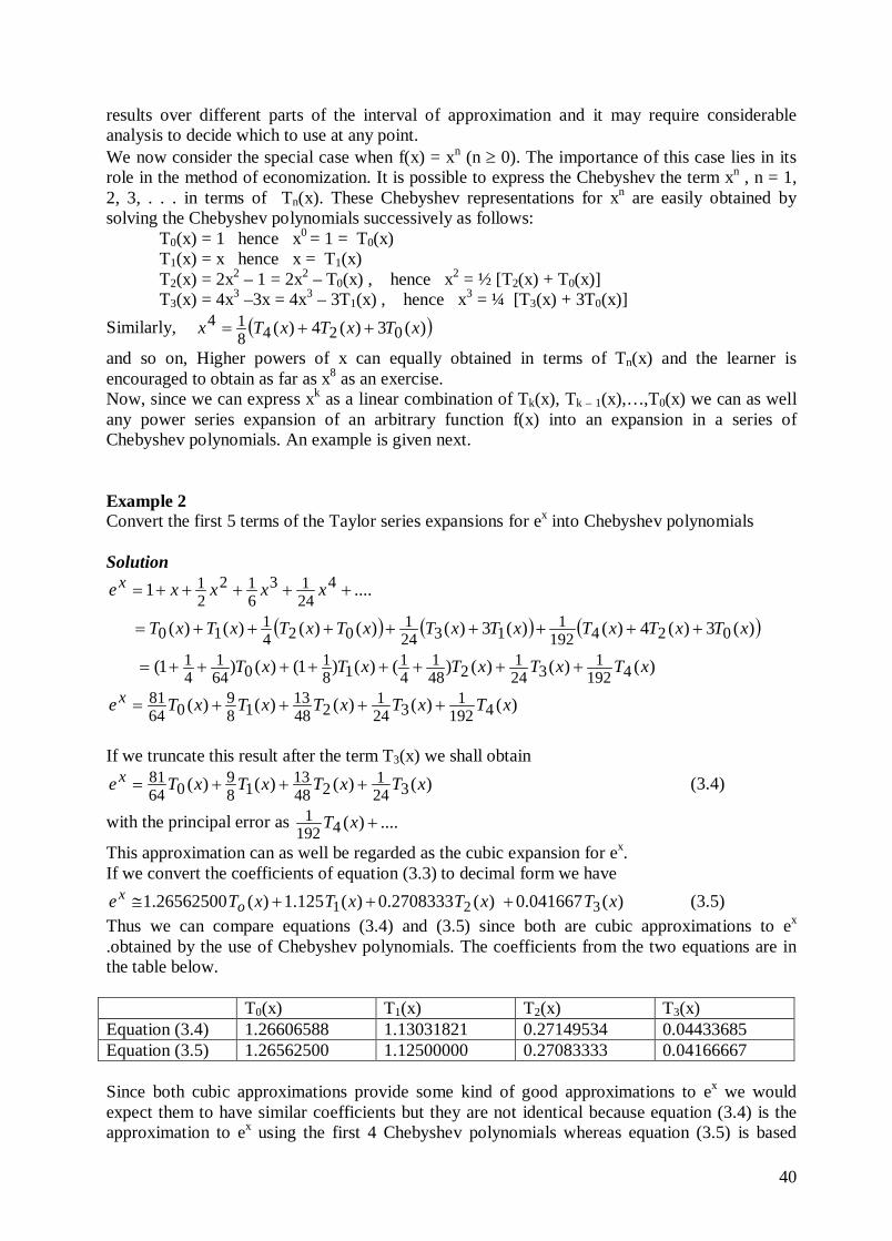
and so on, Higher powers of x can equally obtained in terms of Tn(x) and the learner is encouraged to obtain as far as x8 as an exercise. Now, since we can express xk as a linear combination of Tk(x), Tk – 1(x),…,T0(x) we can as well any power series expansion of an arbitrary function f(x) into an expansion in a series of Chebyshev polynomials. An example is given next. Example 2 Convert the first 5 terms of the Taylor series expansions for ex into Chebyshev polynomials Solution

....1 42413

612

21 +++++= xxxxex

( ) ( ) ( ))(3)(4)()(3)()()()()( 0241921

13241

0241

10 xTxTxTxTxTxTxTxTxT ++++++++=

)()()()()()1()()1( 41921

3241

2481

41

181

0641

41 xTxTxTxTxT ++++++++=

)()()()()( 41921

3241

24813

189

06481 xTxTxTxTxTex ++++=

If we truncate this result after the term T3(x) we shall obtain

)()()()( 3241

24813

189

06481 xTxTxTxTex +++= (3.4)

with the principal error as ....)(41921 +xT

This approximation can as well be regarded as the cubic expansion for ex. If we convert the coefficients of equation (3.3) to decimal form we have

)(041667.0)(2708333.0)(125.1)(26562500.1 321 xTxTxTxTe ox +++≅ (3.5)

Thus we can compare equations (3.4) and (3.5) since both are cubic approximations to ex .obtained by the use of Chebyshev polynomials. The coefficients from the two equations are in the table below. T0(x) T1(x) T2(x) T3(x) Equation (3.4) 1.26606588 1.13031821 0.27149534 0.04433685 Equation (3.5) 1.26562500 1.12500000 0.27083333 0.04166667 Since both cubic approximations provide some kind of good approximations to ex we would expect them to have similar coefficients but they are not identical because equation (3.4) is the approximation to ex using the first 4 Chebyshev polynomials whereas equation (3.5) is based

41

upon the Chebyshev equivalent of the first 5 terms of the Taylor series for ex ‘economized’ to a cubic 4.0 Conclusion It would be observed that as it was done with Legendre polynomials we have similarly obtain a approximate functions to f(x) using the Chebyshev polynomials. The technique of economization is a very useful one and can lead to significant improvements in the accuracy obtainable from a polynomial approximation to a power series. In the next section we present the technique in the general case and in passing see how (3.5) may be more easily obtained. 5.0 Summary In this Unit the reader have learnt that: (i.) Chebyshev polynomials is a technique for approximation using the least square

technique. (ii.) Chebyshev polynomial approach to fitting of approximation to a function is similar to

that of Taylor series for the same function. 6.0 Tutor Marked Assignment (1) Obtain a cubic polynomial to f(x) = 1/x over [-1, 1] by means of Chebyshev polynomials. (2) Convert the first 5 terms of the Taylor series expansions for e–x into Chebyshev

polynomials 7.0 Further Reading and Other Resources

1. Abramowitz M., Stegun I. (eds) ,(1964): Handbook of Mathematical functions, Dover , N.Y.

2. Atkinson K.E. (1978): An Introduction to Numerical Analysis, 2nd Edition, John Wiley & Sons, N.Y

3. Conte S. D. and Boor de Carl Elementary Numerical Analysis an Algorithmic Approach 2nd ed. McGraw-Hill Tokyo.

4. Henrici P. (1982): Essential of Numerical Analysis, Wiley, N.Y 5. Leadermann Walter (1981) (Ed.): Handbook of Applicable Mathematics, Vol 3,

Numerical Analysis, John Wiley, N.Y.

42

MODULE 2 UNIT 6: Chebyshev Interpolation 1.0 Introduction Often we use Lagrange’s methods to interpolate some set of points defined by f(x). the technique is interesting when we involve the use of Chebyshev polynomials. The approach will be discussed in this unit with emphasis on terms such as Lagrange and Chebyshev polynomials. 2.0 Objective By the end of this unit the learner would have learn how to

(i) use Lagrange’s formula (ii) interpolate using Chebyshev polynomials (iii) Compute the error table from the approximation

3.0 Interpolation Technique If the values of a function f(x) are known at a set of points x1 < x2 < … < xn we can construct a polynomial of degree (n – 1) which takes the values f(xi) at xi (i = 1,2,…,n). The polynomial is unique and can be found in various ways including the use of Newton’s divided difference formula or Lagrange’s method. Lagrange’s formula is more cumbersome to use in practice but it has the advantage that we can write down the required polynomial explicitly as:

∑ ∏=

≠= −

−=

n

j

n

iji ij

ij xx

xxxfxp

1 1)()( (3.1)

The reader should note that ∏=

−n

iixx

1)( is a product of function )( ixx − , i = 1, 2, . . ., n, just as

∑=

−n

iixx

1)( is a summation function

Thus ∏=

−n

iixx

1)( is evaluated or expanded as:

)(...))(()( 211

nin

ixxxxxxxx −−−=−∏

=

If f(x) is not a polynomial of degree ≤ (n – 1) the error when we use p(x) for interpolation can be shown to be

∏=

−=n

i

ni n

fxxxE1

)(

!)()()( α

where α is some number between x1 and xn. If the values x1, x2,…xn have been fixed we can do nothing to minimize E(x) but if we can choose any n points within a specified interval it may be worthwhile choosing them in a particular way as we now show Suppose, for simplicity, that we are interested in values of x lying in the interval -1 ≤ x ≤ 1 and that we are free to choose any n points x1, …, xn in this interval for use in the interpolation formula (3.1). Now

∏=

−n

iixx

1)(

43

is a polynomial of degree n with leading coefficient 1 and of all such polynomials the one with the minimum maximum value is )1(2 −− n . It follows therefore that if we wish to minimize (3.1) we should choose the xi so that

1)1(

1 2

)()(.2)(

−−−

===−∏ n

nn

nn

ii

xTxTxx

And this is equivalent to saying that we should choose x1, x2…,xn to be the n roots of Tn(x), that is, we should take ( )πn

mmx

212cos −= , (m = 1 , 2, . . . , n) (3.2)

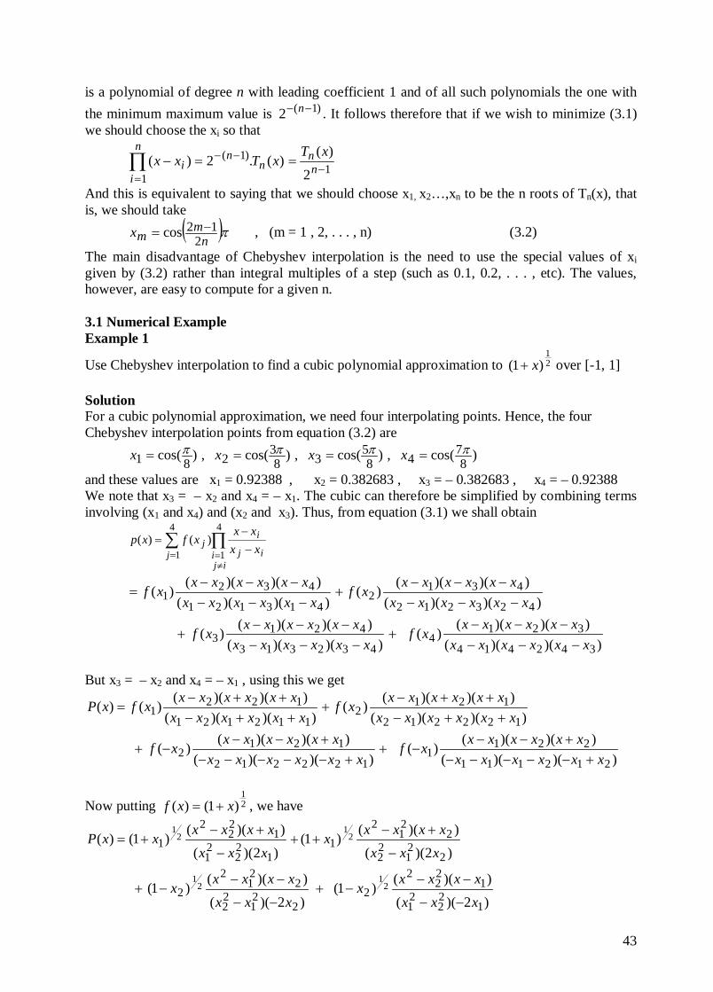
The main disadvantage of Chebyshev interpolation is the need to use the special values of xi given by (3.2) rather than integral multiples of a step (such as 0.1, 0.2, . . . , etc). The values, however, are easy to compute for a given n. 3.1 Numerical Example Example 1

Use Chebyshev interpolation to find a cubic polynomial approximation to 21

)1( x+ over [-1, 1] Solution For a cubic polynomial approximation, we need four interpolating points. Hence, the four Chebyshev interpolation points from equation (3.2) are

)cos(,)cos(,)cos(,)cos(8

748

538

3281

ππππ ==== xxxx

and these values are x1 = 0.92388 , x2 = 0.382683 , x3 = – 0.382683 , x4 = – 0.92388 We note that x3 = – x2 and x4 = – x1. The cubic can therefore be simplified by combining terms involving (x1 and x4) and (x2 and x3). Thus, from equation (3.1) we shall obtain

∑ ∏=

≠= −

−=

4

1

4

1)()(

jij

i ij

ij xx

xxxfxp

))()(())()((

)())()((

))()(()(

))()(())()((

)())()((

))()(()(

342414

3214

432313

4213

423212

4312

413121

4321

xxxxxxxxxxxx

xfxxxxxx

xxxxxxxf

xxxxxxxxxxxx

xfxxxxxx

xxxxxxxf

−−−−−−

+−−−

−−−+

−−−−−−

+−−−

−−−=

But x3 = – x2 and x4 = – x1 , using this we get

))()(())()(()(

))()(())()(()(

))()(())()(()(

))()(())()(()()(

212111

2211

122212

1212

122212

1212

112121

1221

xxxxxxxxxxxxxf

xxxxxxxxxxxxxf

xxxxxxxxxxxxxf

xxxxxxxxxxxxxfxP

+−−−−−+−−

−++−−−−−

+−−−+

++−++−

+++−

++−=

Now putting 21

)1()( xxf += , we have

)2)((

))(()1()2)((

))(()1(

)2)((

))(()1()2)((

))(()1()(

122

21

122

22

221

22

221

22

221

22

221

21

122

21

122

21

21

21

21

21

xxxxxxxx

xxxxxxxx

xxxxxxxx

xxxxxxxxxP

−−

−−−+

−−

−−−+

−

+−++

−

+−+=

44

Substituting for x1 and x2 we obtain

) 0.923882)(0.3826830.92388() 0.92388)(0.382683(

) 0.3826831(

) 0.3826832)(0.923880.382683() 0.382683)(0.92388(

) 0.3826831(

) 0.3826832)(0.923880.382683() 0.382683)(0.92388(

) .923881(

) 0.923882)(0.382683 0.92388() 0.92388)(0.382683(

).923881()(

22

22

22

22

22

22

22

22

21

21

21

21

×−−

−−−+

×−−

−−−+

×−

+−+

×−

+−=

xx

xx

xx

xxxP

) 84776.1)(0.1464460.853554() 0.92388)(0.146446()785695.0(

) .7653660)(0.853554(0.146446) 0.382683)(0.853554()785695.0(

) .7653660)(0.8535540.146446() 0.382683)( 0.853554().387021(

) 84776.1)(0.146446 0.853554() 0.92388)(0.146446().387021()(

2

2

2

2

−−−−

×+

−−−−

×+

−+−

×+

−+−

×=

xx

xx

xx

xxxP

) 0.92388)(0.146446()6013436.0(

) 0.382683)(0.853554()6383371.2(

) 0.382683)( 0.853554()5628773.2(

) 0.92388)(0.146446().06157691()(

2

2

2

2

−−×−+

−−×+

+−×−+

+−×=

xx

xx

xx

xxxP

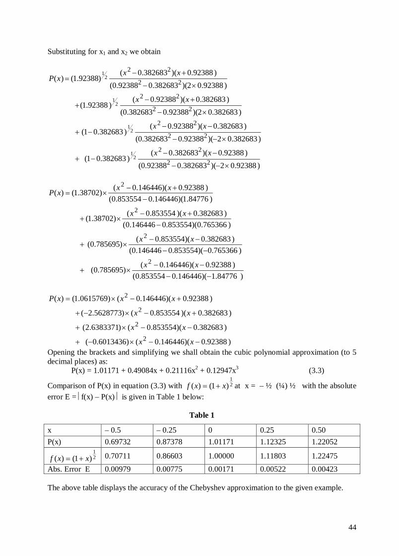
Opening the brackets and simplifying we shall obtain the cubic polynomial approximation (to 5 decimal places) as: P(x) = 1.01171 + 0.49084x + 0.21116x2 + 0.12947x3 (3.3)

Comparison of P(x) in equation (3.3) with 21

)1()( xxf += at x = – ½ (¼) ½ with the absolute error E = f(x) – P(x) is given in Table 1 below:

Table 1

x – 0.5 – 0.25 0 0.25 0.50 P(x) 0.69732 0.87378 1.01171 1.12325 1.22052

21

)1()( xxf += 0.70711 0.86603 1.00000 1.11803 1.22475

Abs. Error E 0.00979 0.00775 0.00171 0.00522 0.00423 The above table displays the accuracy of the Chebyshev approximation to the given example.

45

4.0 Conclusion We have been able to demonstrate the use of Lagrange’s method in our interpolation technique. We have also seen that Chebyshev polynomials are of great usefulness in the interpolation of simple functions. 5.0 Summary In this Unit the reader have learnt that: (i.) interpolation technique is possible by using Chebyshev polynomials. (ii.) Lagrange’s method of interpolating is basic and very useful. (ii) the difference of the actual and the approximate value is the error 6.0 Tutor Marked Assignment

Use Chebyshev interpolation technique to find a cubic polynomial approximation to 21

)1(−

− x

over [-1, 1] 7.0 Further Reading and Other Resources

1. Atkinson K.E. (1978): An Introduction to Numerical Analysis, 2nd Edition, John Wiley & Sons, N.Y

2. Conte S. D. and Boor de Carl Elementary Numerical Analysis an Algorithmic Approach 2nd ed. McGraw-Hill Tokyo.

3. Francis Scheid. (1989) Schaum’s Outlines Numerical Analysis 2nd ed. McGraw-Hill New York.

4. Henrici P. (1982): Essential of Numerical Analysis, Wiley, N.Y 5. Kandassamy P., Thilagarathy K., & Gunevathi K. (1997) : Numerical Methods, S. Chand

& Co Ltd, New Delhi, India 6. Leadermann Walter (1981) (Ed.): Handbook of Applicable Mathematics, Vol 3,

Numerical Analysis, John Wiley, N.Y. 7. Turner P. R. (1994) Numerical Analysis Macmillan College Work Out Series Malaysia

46

MODULE 3

FURTHER INTERPOLATION TECHNIQUES

UNIT 1: CUBIC SPLINE INTERPOLATION 1.0 Introduction

One of the problems which frequently arises when we try to approximate a function by means of a polynomial of high degree is that the polynomial turns out to have closed placed maxima and minima, thus giving it an undulatory (or ‘wiggly’) character. This is very undesirable if the polynomial is to be used for interpolation, and disastrous if it is to be used for numerical differentiation. In 1945, I. J. Schoenberg introduced the idea of approximation to functions by means of a series of polynomials over adjacent intervals with continuous derivatives at the end-points of the intervals. Such a set of polynomials he called ‘splines’, pointing out that architects and designers had been using mechanical devices of this kind for years. In his paper Schoenberg explains. A spline is a simple mechanical device for drawing smooth curves. It is a slender flexible bar made of wood or some other elastic materials. The spline is placed on the sheet of graph paper and held in place at various points.. The mathematical equivalent of this ‘flexible bar’ is the cubic spline which has proved to be extremely useful for interpolation, numerical differentiation and integration and has been subject of many research papers. 2.0 Objective By the end of this unit, the learner should be able to:

(f) define a cubic spline; (g) derive a method of fitting a cubic spline; (h) fit a cubic spline to set of data points; (i) interpolate a function from the fitted cubic spline; (j) find the error in the cubic spline.

3.0 Spline Function To be able to understand this module we shall begin the discussion by defining what is meant by splines of degree k and then develop the special case of the cubic (k = 3) Definition 1 A spline function S(x) of degree k with n nodes, x1 < x2 < … < xn has the properties

(i.) S(x) is given in the interval [xi , xi+1] , i = 0, 1, . . . , n (where xo = – ∞ , xn+1 = ∞) by a polynomial of degree at most k (in general, a different polynomial is obtained in each interval);

(ii.) S(x) and all derivatives of orders 1, 2, …, k–1 are continuous on (– ∞ , ∞) In the case k = 3, the polynomials in each of the intervals are at most cubics and their first and second derivatives are continuous at the end points of the intervals. Such a set of polynomials form a cubic spline. We can narrow down this definition to a cubic spline S(x) as follows:

47

Definition 2 A Cubic Spline S(x) is a function which satisfies the following properties S(x) is a polynomial of degree one for x < x0 and x > xn S(x) is at most a cubic polynomial in (xi, xi+1) , i = 0, 1, 2,. . . , n – 1; S(x) , S′(x) and S″(x) are continuous at each point (xi , yi) , i = 0, 1, 2,. . . , n; S(xi) = yi , i = 0, 1, 2,. . . , n. 3.1 Derivation of Cubic Spline How can we construct a cubic spline? How many data points or set is required? We shall give simple and interesting, with step by step procedure of derivation of cubic splines. We proceed as follows: Suppose that we are given a set of points x1 < x2 < … < xn, not necessary equally spaced, and a set of values f(x1), f(x2),…, f(xn) at these points. Take a particular interval [xi, xi + 1] and fit a cubic over the interval which satisfies the definition of a cubic spline. Since the cubic may differ from one interval to another let the cubic be

S(x) = 13

32

21 ,)( +≤≤+++= iioi xxxxaxaxaaxP (3.1) Equation (3.1) contains 4 unknowns. We impose 2 obvious conditions

,)( iii yxP = and 11 )( ++ = iii yxP . The remaining 2 conditions are obtained by choosing the coefficients so that the first and second derivatives of Pi(x) at x, are equal to the first and second derivatives of Pi+1(x) at xi , that is

)()()()(

1

1

iiii

iiiixPxPxPxP

+

+′′=′′′=′

There remain special problem at x1 and xn, but we will deal with these later. The conditions are now sufficient to determine the (n – 1) cubics which collectively constitute the cubic spline S(x) that is:

1)()( +≤≤= iii xxxforxPxS How can we solve these equations? The simplest method is to note that S″(x) is linear in x and is also continuous over the whole interval [x1, xn]. S″ (x) can therefore be represented in [xi, xi + 1] by a linear function which is only seen to be

[ ])()()()( 11

iiii

ii xSxS

xxxx

xSxS ′′−′′−

−−′′=′′ +

+ (3.2)

We rewrite (3.2) in the form

)()()(1

11

1i

iii

iii

i xSxx

xxxS

xxxx

xS ′′−

−−′′

−−

=′′+

++

+ (3.3)

We integrate twice then, putting h = hi = xi+1 – xi as usual, the result can be written as

axSh

xxxS

hxx

xS ii

ii +′′−

−′′−= +

+ )(6

)()(

6)(

)(3

11

3(x – xi) +b(x – xi+1) (3.4)

Hence any expression of the form Ax + B may be written as a(x – xi) +b(x – xi+1) for suitable choice of a,b provided 1+≠ ii xx We now impose the conditions that ii yxS =)( and 11)( ++ = ii yxS so that on putting x = xi , equation (3.4) becomes

48

)()(6

)(1

31

++ −+′′−−

= iiiii

i xxbxShxx

y (3.5)

bhxSh

hy ii −′′= )(6

3

⇒ )(6

2ii xShybh ′′+−=

)(6 i

i xShhy

b ′′+−

= (3.6)

Also putting x = xi+1 in equation (3.4) , we get

ahxSh

hy ii +′′= ++ )(6 1

31

or )(6 1

1+

+ ′′−= ii xShh

ya (3.7)

Substituting equations (3.6) and (3.7) in equation (3.4) gives:

′′+−

−+

′′−−+

′′−−′′−

=

+++

++

)(6

)()(6

)(

)(6

)()(

6)(

)(

111

31

13

ii

iii

i

ii

ii

xShhy

xxxShh

yxx

xSh

xxxS

hxx

xS

after slight re-arrangement of terms, we obtain

−+

−+

−−

−′′+

−−

−′′=

++

++

+

hxx

yh

xxy

xxhhxxxS

xxhh

xxxSxS

ii

ii

iii

iii

)()(

)()(

6)(

)()(

6)(

)(

11

31

13

1

(3.8)

This expression is valid for the interval xi < x < xi+1 It is worth noting that if in (3.8) we ignore the two terms involving S″(xi) and S″(xi+1) we obtain the approximation to S(x)

ih

yxxyxxxS iiii 11 )()()( ++ −−−≅

which is the result for linear interpolation. We see therefore that the terms involving S″(xi) and S″(xi+1) can be regarded as correction terms obtained by using a cubic instead of a linear approximation. Before we can use (3.8) to determine S(x) we must find the values S″(xi) and this we do by using the conditions that the first derivatives are continuous at the nodes. Differentiating (3.8) and putting x = xi we have

hy

xyxSh

hh

xxxSxS i

iiiiii

i11

21

6)()(3

6)(

)( +++ +−′′

−

+

−−

′′=′ (3.9)

If we now replace i by (i – 1) in equation (3.8), differentiate and again put x = xi , we obtain

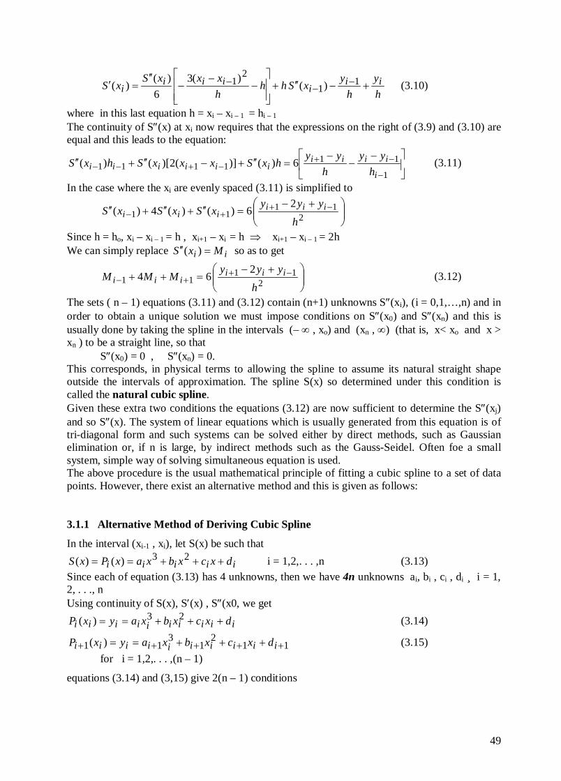
49

hy

hy

xShhhxxxS

xS iii

iiii +−′′+

−

−−

′′=′ −

−− 1

12

1 )()(3

6)(

)( (3.10)

where in this last equation h = xi – xi – 1 = hi – 1 The continuity of S″(x) at xi now requires that the expressions on the right of (3.9) and (3.10) are equal and this leads to the equation:

−−

−=′′+−′′+′′

−

−+−+−−

1

111111 6)()](2)[()(

i

iiiiiiiiii h

yyh

yyhxSxxxShxS (3.11)

In the case where the xi are evenly spaced (3.11) is simplified to

+−=′′+′′+′′ −+

+− 211

112

6)()(4)(h

yyyxSxSxS iii

iii

Since h = ho, xi – xi – 1 = h , xi+1 – xi = h ⇒ xi+1 – xi – 1 = 2h We can simply replace ii MxS =′′ )( so as to get

+−=++ −+

+− 211

112

64h

yyyMMM iii

iii (3.12)

The sets ( n – 1) equations (3.11) and (3.12) contain (n+1) unknowns S″(xi), (i = 0,1,…,n) and in order to obtain a unique solution we must impose conditions on S″(x0) and S″(xn) and this is usually done by taking the spline in the intervals (– ∞ , xo) and (xn , ∞) (that is, x< xo and x > xn ) to be a straight line, so that

S″(x0) = 0 , S″(xn) = 0. This corresponds, in physical terms to allowing the spline to assume its natural straight shape outside the intervals of approximation. The spline S(x) so determined under this condition is called the natural cubic spline. Given these extra two conditions the equations (3.12) are now sufficient to determine the S″(xj) and so S″(x). The system of linear equations which is usually generated from this equation is of tri-diagonal form and such systems can be solved either by direct methods, such as Gaussian elimination or, if n is large, by indirect methods such as the Gauss-Seidel. Often foe a small system, simple way of solving simultaneous equation is used. The above procedure is the usual mathematical principle of fitting a cubic spline to a set of data points. However, there exist an alternative method and this is given as follows: 3.1.1 Alternative Method of Deriving Cubic Spline

In the interval (xi-1 , xi), let S(x) be such that

iiiii dxcxbxaxPxS +++== 23)()( i = 1,2,. . . ,n (3.13) Since each of equation (3.13) has 4 unknowns, then we have 4n unknowns ai, bi , ci , di ¸ i = 1, 2, . . ., n Using continuity of S(x), S′(x) , S″(x0, we get

iiiiiiiiii dxcxbxayxP +++== 23)( (3.14)

112

13

11 )( +++++ +++== iiiiiiiiii dxcxbxayxP (3.15) for i = 1,2,. . . ,(n – 1)

equations (3.14) and (3,15) give 2(n – 1) conditions

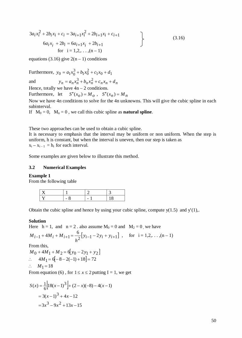
50

11

112

12

2626

2323

++

+++

+=+

++=++

iiiiii

iiiiiiiiii

bxabxa

cxbxacxbxa (3.16)

for i = 1,2,. . . ,(n – 1)

equations (3.16) give 2(n – 1) conditions Furthermore, 101

201

3010 dxcxbxay +++=

and nnnnnnnn dxcxbxay +++= 23 Hence, totally we have 4n – 2 conditions. Furthermore, let nnoo MxSMxS =′′=′′ )(,)( Now we have 4n conditions to solve for the 4n unknowns. This will give the cubic spline in each subinterval. If M0 = 0, Mn = 0 , we call this cubic spline as natural spline. These two approaches can be used to obtain a cubic spline. It is necessary to emphasis that the interval may be uniform or non uniform. When the step is uniform, h is constant, but when the interval is uneven, then our step is taken as xi – xi – 1 = hi for each interval. Some examples are given below to illustrate this method. 3.2 Numerical Examples

Example 1 From the following table

X 1 2 3 Y - 8 - 1 18

Obtain the cubic spline and hence by using your cubic spline, compute y(1.5) and y′(1),. Solution Here h = 1, and n = 2 . also assume M0 = 0 and M2 = 0 , we have

[ ]11211 264 +−+− +−=++ iiiiii yyyh

MMM , for i = 1,2,. . . ,(n – 1)

From this, [ ]210210 264 yyyMMM +−=++

∴ [ ] 7218)1(2864 1 =+−−−=M ∴ 181 =M From equation (6) , for 21 ≤≤ x putting I = 1, we get

[ ] )1(4)8)(2()1(18)( 361 −−−−+−= xxxxS

151393

124)1(323

3

−+−=

−+−=

xxx

xx

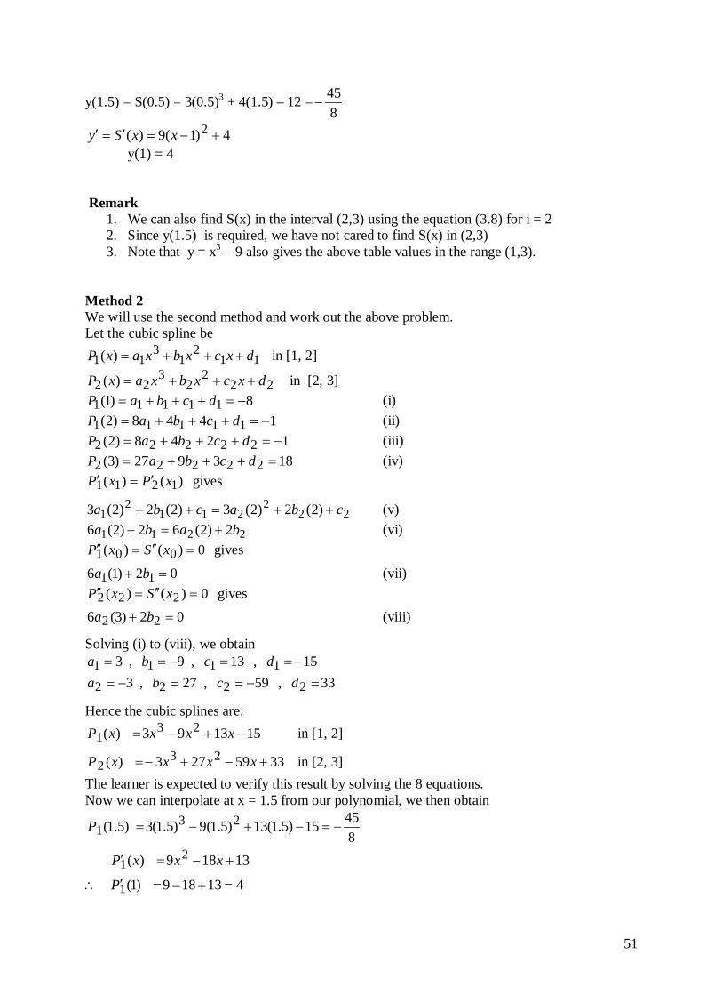
51

y(1.5) = S(0.5) = 3(0.5)3 + 4(1.5) – 12 =845

−

4)1(9)( 2 +−=′=′ xxSy y(1) = 4 Remark

1. We can also find S(x) in the interval (2,3) using the equation (3.8) for i = 2 2. Since y(1.5) is required, we have not cared to find S(x) in (2,3) 3. Note that y = x3 – 9 also gives the above table values in the range (1,3).

Method 2 We will use the second method and work out the above problem. Let the cubic spline be

112

13

11 )( dxcxbxaxP +++= in [1, 2]

222

23

22 )( dxcxbxaxP +++= in [2, 3] 8)1( 11111 −=+++= dcbaP (i)

1448)2( 11111 −=+++= dcbaP (ii) 1248)2( 22222 −=+++= dcbaP (iii) 183927)3( 22222 =+++= dcbaP (iv)

)()( 1211 xPxP ′=′ gives

222

2112

1 )2(2)2(3)2(2)2(3 cbacba ++=++ (v)

2211 2)2(62)2(6 baba +=+ (vi) 0)()( 001 =′′=′′ xSxP gives

02)1(6 11 =+ ba (vii) 0)()( 222 =′′=′′ xSxP gives

02)3(6 22 =+ ba (viii)

Solving (i) to (viii), we obtain

33,59,27,315,13,9,3

2222

1111=−==−=

−==−==dcba

dcba

Hence the cubic splines are: 151393)( 23

1 −+−= xxxxP in [1, 2]

3359273)( 232 +−+−= xxxxP in [2, 3]

The learner is expected to verify this result by solving the 8 equations. Now we can interpolate at x = 1.5 from our polynomial, we then obtain

84515)5.1(13)5.1(9)5.1(3)5.1( 23

1 −=−+−=P

413189)1(

13189)(

1

21

=+−=′∴

+−=′

P

xxxP

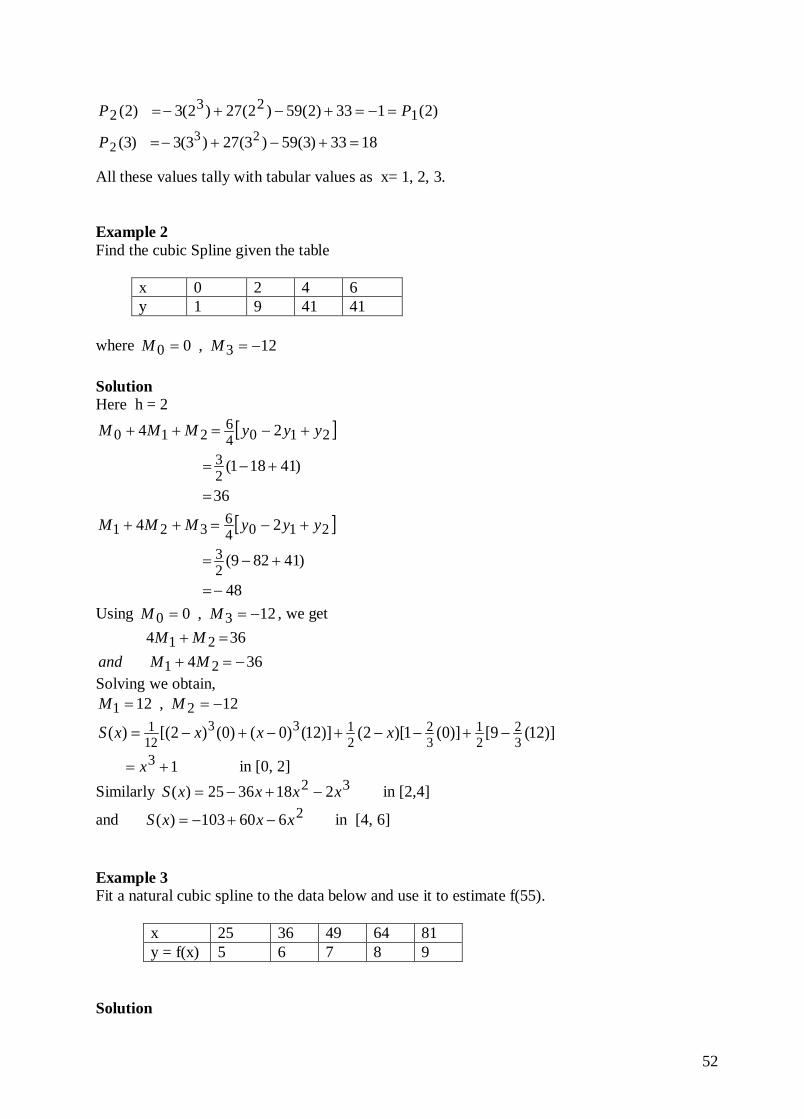
52

)2(133)2(59)2(27)2(3)2( 123

2 PP =−=+−+−=

1833)3(59)3(27)3(3)3( 232 =+−+−=P

All these values tally with tabular values as x= 1, 2, 3. Example 2 Find the cubic Spline given the table

x 0 2 4 6 y 1 9 41 41

where 12,0 30 −== MM Solution Here h = 2

[ ]

36

)41181(

24

23

21046

210

=

+−=

+−=++ yyyMMM

[ ]

48

)41829(

24

23

21046

321

−=

+−=

+−=++ yyyMMM

Using 12,0 30 −== MM , we get

364364

21

21−=+

=+MMandMM

Solving we obtain, 12,12 21 −== MM

)]12(9[)]0(1)[2()]12()0()0()2[()( 32

21

32

2133

121 −+−−+−+−= xxxxS

13 += x in [0, 2] Similarly 32 2183625)( xxxxS −+−= in [2,4]

and 2660103)( xxxS −+−= in [4, 6] Example 3 Fit a natural cubic spline to the data below and use it to estimate f(55).

x 25 36 49 64 81 y = f(x) 5 6 7 8 9

Solution

53

We use (3.11) to form a set of linear equations for S″(36), S″(49), S″(64) and we take S″(25) = S″(81) = 0. The equations are )(6)49(13)36()24(211).0(

111

131 −=′′+′′+ SS

)(6)64(15)49()28(2)36(.13131

151 −=′′+′′+′′ SSS

)(6)0(17)64()32(2)49(.15151

171 −=+′′+′′ SS

Let cSbSaS =′′=′′=′′ )64(,)49(,)36( , we re-write the equations in terms of a, b, c as

143

121348 −=+ ba

195121556.13 −=++ cba

2551264.15 −=+ cb

Solving these equations simultaneously we obtain a = S″(36) = – 0.001594 b = S″(49) = – 0.000568, c = S″(64) = – 0.000602 The point at which we wish to interpolate, x = 55, lies in the interval [49, 64] and we must use the cubic appropriate to that interval, i.e. we use equation (3.8) when xi+1 = 64, xi = 49, x = 55 and so we obtain

−

+

−

+

−−

−′′+

−−

−′′=

15)4955(8

15)5564(7

)4955(1515

)4955(6

)64()5564(1515

)5564(6

)49()55(33 SSS

i.e. S(55) = 0.008179 – 0.007585 + 7.4 = 7.415764 So our estimate for f(55) is 7.415764 As remarked above the last two terms constitute the linear approximation which therefore has the value ( ) ( ) 4.787

156

159 =−

Since the function, f(x) is in fact x we can check on the accuracy of the estimate. The error E of our cubic spline is obtained by taking the difference from the exact value Now 416198.755 = Hence E = 7.416198 – 7.415764 = 0.000434 And the error of the linear approximation is E1 = 7.416198 – 7.4 = 0.016198 Thus the linear estimate is correct to only 1 d.p. while the cubic spline turns out to be correct to 3 d.p. with little error of 4.34 ×10 – 4 The result is satisfactory because we are working near the middle of a range of a smooth function with a small (absolute) value for its second derivative. Remember that we have taken S″(25) = S″(81) = 0. Self Assessment Exercise 1. Can you find S(x) in the interval (2,3) for i = 2 in Example 1 above, using the same method.

54

4.0 Conclusion Cubic spline has a great advantage of fitting polynomial of degree three simply by using the above techniques. It will be cumbersome to think of fitting a polynomial of higher degree as this will require deriving a set of formula as it was done in section 3.1. However, it is known that a cubic spline gives a good accuracy to several functions that permits polynomial fitting. 5.0 Summary In this Unit we have learnt (i) how to derive the cubic spline formula involving set of linear equations (ii) how to fit a cubic spline or polynomial of degree three to a set of data points using cubic

spline technique. (iii) that cubic spline have good accuracy with minimum error when used to fit a function. 6.0 Tutor Marked Assignment Fit a natural cubic spline to the data below and use it to estimate f(24).

x 10 15 20 25 30 y = f(x) 8 10 12 15 18

7.0 Further Reading and Other Resources

1. Abramowitz M., Stegun I. (eds) ,(1964): Handbook of Mathematical functions, Dover , N.Y.

2. De Boor C. (1978) : A Practical Guide to Splines, Springer Verlag, N.Y. 3. Francis Scheid. (1989) Schaum’s Outlines Numerical Analysis 2nd ed. McGraw-Hill New

York. 4. Kandassamy P., Thilagarathy K., & Gunevathi K. (1997) : Numerical Methods, S. Chand

& Co Ltd, New Delhi, India 5. Leadermann Walter (1981) (Ed.): Handbook of Applicable Mathematics, Vol 3,

Numerical Analysis, John Wiley, N.Y. 6. Turner P. R. (1994) Numerical Analysis Macmillan College Work Out Series Malaysia

55

MODULE 3 UNIT 2 HERMITE APPROXIMATIONS 1.0 Introduction For approximation, or interpolation, of a function defined analytically a method due to Hermite is often useful. The method is superficially related to the spline method but in fact the two methods are very different because fitting of spline involves solving a system of linear equations to obtain numerical values for the second derivatives. S″(xi), whereas for Hermite interpolation the values of the first derivatives are given, and the second derivatives are not relevant Spline are mainly used for fitting polynomials to data, Hermite polynomials are mainly used for approximating to functions The most commonly used Hermite approximation polynomial is the cubic, as in the case of spline and we shall discuss only this case in detail, the more general case can be analyzed in a similar manner. 2.0 Objective By the end of this unit, the learner should be able to:

(i) distinguish between cubic spline and Hermite polynomial (ii) figure out the Hermite approximation formula (iii) fit polynomial by Hermite approximation technique and find an estimate.

3.0 Hermite Approximation Formula Suppose we have an analytic function y = f(x) with values f(xi) and derivatives f’(xi) given at n points xi (i = 1,…,n). Across each pair of adjacent points xm, xm+1 we fit a cubic pm(x) such that

)()(,)()()()(,)()(

1111 ++++ ′=′=

′=′=

mmmmmm

mmmmmmxfxpxfxp

xfxpxfxp

Since pm(x) contains 4 coefficients, then four necessary equations will determine it uniquely, and indeed the formula for pm(x) can be explicitly stated as:

( )( )( )

( ) ( )( )

)()(

)(21)(21)(

121

12

21

21

1

2

111

2

11

1

++

+

+

+

+++

+

+

+

+

′−

−−+′

−

−−+

−

−

−−

++

−−

−

−+=

mmm

mmm

mm

mm

mmm

mmm

mm

mmm

mmm

m

xfxx

xxxxxf

xx

xxxx

xfxx

xxxxxx

xfxxxx

xxxx

xp(3.1)

A cubic Hermite approximation thus consists of a set of cubic polynomials; each defined over one interval, with continuity of the cubics and their first derivatives at all the nodes. An example will be given to illustrate how this is used. This formula is not difficult to know, all it required is the placement of each subscript of x. 3.1 Numerical Example Example 1 Use Hermite cubic interpolation to estimate the value of 55 taking xxf =)( , x1 = 49, x2 = 64 Solution

Given xxf =)( then x

xf2

1)( =′

56

From (3.1) with xm = 49, xm+1 = 64, 749)( ==mxf , 141

4921)( ==′ mxf ,

Similarly, 161

6421)(,864)( 11 ==′== ++ mm xfxf

we have the Hermite cubic approximation as

( )( )( )

( ) ( ) ( )( )

( )161

2

2

141

2

2

22

4964

6449

4964

6449

)8(496449

49646421)7(

496464

49644921)(

−

−−+

−

−−+

−−

−−

×++

−−

−−

×+≅

xxxx

xxxxxf

( )( ) ( ) ( )162256449

142256449)8(

1549

152143)7(

1564

15832 2222

×−−

+×

−−+

−

−

+

−

−

=xxxxxxxx

This gives the required Hermite polynomial approximation to xxf =)( . We may simplify this as much as possible. However, since we are only to estimate the square root of 55, simplifying this expression may not be all that necessary until we have substituted the value for x. Hence, putting x = 55 in the last equation obtained yields the estimate

7.41628655 ≅ The correct value of 55 to 6 d.p is 7416198, so the error is 0.000088 compared to an error of -.000434 when we used the natural cubic spline in Example 3 of Unit 1 4.0 Conclusion In general the errors when we use the Hermite cubic and the natural cubic spline on the same problem will not be very different for in both cases the error is proportional to h4 where h is the step between the two relevant nodes. 5.0 Summary In this Unit we have learnt that

(i) Hermite approximation differs from cubic. (ii) cubic spline fit a polynomial to a set of data points while Hermite approximate a

function as a polynomial. (iii) Hermite approximation may be more accurate than the cubic spline.

6.0 Tutor Marked Assignment Obtain an Hermite approximation of polynomial of degree 3 to the function f(x) = ln x for x1 = 2, x2 = 5 and hence estimate the value of ln 3.5 7.0 Further Reading and Other Resources 1. Abramowitz M., Stegun I. (eds) ,(1964): Handbook of Mathematical functions, Dover , N.Y. 2. Atkinson K.E. (1978): An Introduction to Numerical Analysis, 2nd Edition, John Wiley & Sons, N.Y 3. Conte S. D. and Boor de Carl Elementary Numerical Analysis an Algorithmic Approach 2nd ed.

McGraw-Hill Tokyo. 4. Francis Scheid. (1989) Schaum’s Outlines Numerical Analysis 2nd ed. McGraw-Hill New York. 5. Henrici P. (1982): Essential of Numerical Analysis, Wiley, N.Y 6. Kandassamy P., Thilagarathy K., & Gunevathi K. (1997) : Numerical Methods, S. Chand & Co Ltd,

New Delhi, India 7. Turner P. R. (1994) Numerical Analysis Macmillan College Work Out Series Malaysia

57

MODULE 4

NUMERICAL INTEGRATION

UNIT 1 INTRODUCTION TO NUMERICAL INTEGRATION 1.0 Introduction In numerical analysis, integration seems to be easier than differentiation, which is the reverse in Calculus. Hence the cases where most integrals have no representation in terms of elementary function will only require the use of approximation functions. This is done by the process of numerical integration. The importance of numerical integration is clearly seen when we consider how frequently derivatives are involved in the formulation of problems in applied analysis. It is well observed that polynomial approximation serves as the basis for a variety of integral formulas, hence the need to have studied some polynomial approximation techniques. 2.0 Objective At the end of this Unit, the learner would have learn

(i) what numerical integration is all about (ii) differentiate between analytical approach and numerical approach to integration (iii) be able to list various known methods for numerical quadrature

3.0 Quadrature In the study elementary calculus especially integration, there are various techniques involved to evaluate different kind of integrals. Some integral are cumbersome that sometimes are left in form of another integral in a sense. There are several other ones that need the help of special functions or reduction of order before they can be evaluated. This is one reason why numerical integration comes to play a role in the evaluation of such integrals. The main procedure of numerical integration is to divide the range of interval of integration into some equal intervals and obtain the integral of the first strip of the interval. Upon the first result, other strips are generalized. The other strips after the first are to correct the accuracy of the first, thereby quadraturing the strips one after the other. Hence, Numerical integration is commonly referred to as Numerical quadrature and their formulas are called quadrature formulas. It is worth noting that results or formulas derived in this way are also termed as rules rather than methods. Thus, we talk of Trapezoidal rule, Simpson’s rules, Newton-Cotes rules, etc. The main idea is, if P(x) is an approximation to y(x) then

∫∫ ≈ba

ba

dxxydxxP )()( (3.1)

That is the integral of P(x) can be approximated by some numerical schemes which consider some points within the limits of integration. These points are node points or collocating points which are subdivided into by equal spacing on the x –axis. Thus if the range or limits of integration which is [a, b] are actually points [x0, xn], then the interval [x0, xn] can be subdivided into equal interval as shown below Now between any successive interval, is what is called the step length denoted by h, so that

h = x1 – xo = x2 – x1 = x3 – x2 = . . . . = xn – xn-1 ⇒ xn = xo + nh

x0 x1 x2 . . . . xn-1 xn

58

3.1 Quadrature Formulas There are standard rules in numerical analysis that can be used to estimate the above integral. Among such rules or formulas are:

(i.) Trapezoidal rule, (ii.) Simpson’s

31 - rule,

(iii.) Simpson’s −83 rule,

(iv.) Newton – Cotes formulas The Trapezoidal rule is given by

)2.....22( )( 121021

0nn

nxx

yyyyyhdxxP +++++= −∫

The Simpson’s 31 - rule is given by

)42.....2424( )( 124321031

nnnnx

oxyyyyyyyyhdxxP ++++++++= −−∫

While the Simpson’s −83 rule is given by

( )nnnx

xyyyyyyyyyydxxP

n++++++++++= −−∫ 1265432108

3 3 3 ...23 3 23 3 h )(0

The Newton – Cotes formulas depend on the value of n starting from n = 4 ,6, . . . The derivations of these formulas are very essential to the learning of Numerical integration. While they are interesting in the learning of the topic, it also helps in the understanding of the workings of these formulae rather than trying to memorize them. Thus attempt will be made to give the required techniques of their derivations and the learner will complete the rest. 3.2 Newton Gregory Formula The most acceptable way of deriving all these rules listed above is by using the Newton forward formula or Newton backward formula. However we shall restrict our learning to using the Newton Forward formula for deriving the integration formula in this course. Geometrically the Trapezoidal rule which sometimes is simply called the trapezium formula can be derived by approximating a curve by a straight line, thereby getting a trapezium. The Newton Gregory Forward formula is given by Pk(x) = y0 + kC1∆y0 + kC2 ∆2 y0 + kC3 ∆3 y0 + …. + kCn ∆n y0 (3.2)

0!))....(2)(1(

03

!3)2)(1(

02

!2)1(

00 ... yyyyky nn

nkkkkkkkkk ∆++∆+∆+∆+= −−−−−−

Integrating this formula of degree n between xo and xn gives several useful quadrature formulas. where ∆ is a forward difference operator defined as ∆yk = yk+1 - yk This formula (3.2) is very useful in the derivation of all numerical integration schemes. The accuracy of these quadrature formulas differs when applied to a definite integral. The smaller the stripe h is, the better the accuracy. It must be mentioned here that numerical integration deals with only definite integrals. In other words, indefinite integrals are best handled by analytical means. However in practice, most practical problems involve definite integrals and so numerical integration is very relevant in physical and day to day problems. Each of these formulas will be discussed in subsequent Units.

59

4.0 Conclusion The use of quadrature formulas are of high importance to this study. We have introduced all the relevant formulas which we shall later use to evaluate some definite integrals. 5.0 Summary In this Unit we have learnt that (i) quadrature is a numerical analysis terminology that refers to numerical integration (ii) there are three standard numerical integration formulas viz: Trapezoidal rule, Simpson’s

rules and Newton – Cotes formulas (ii) Newton Gregory formula is the basis for the derivation of these quadrature formulas. 6.0 Tutor Marked Assignment Use geometrical approach r to derive the trapezoidal rule. 7.0 Further Reading and Other Resources

1. Francis Scheid. (1989) Schaum’s Outlines Numerical Analysis 2nd ed. McGraw-Hill New York.

2. Kandassamy P., Thilagarathy K., & Gunevathi K. (1997) : Numerical Methods, S. Chand & Co Ltd, New Delhi, India

3. Leadermann Walter (1981) (Ed.): Handbook of Applicable Mathematics, Vol 3, Numerical Analysis, John Wiley, N.Y.

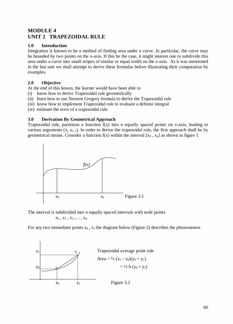
60

MODULE 4 UNIT 2 TRAPEZOIDAL RULE 1.0 Introduction Integration is known to be a method of finding area under a curve. In particular, the curve may be bounded by two points on the x-axis. If this be the case, it might interest one to subdivide this area under a curve into small stripes of similar or equal width on the x-axis. As it was mentioned in the last unit we shall attempt to derive these formulas before illustrating their computation by examples. 2.0 Objective At the end of this lesson, the learner would have been able to (i) know how to derive Trapezoidal rule geometrically (ii) learn how to use Newton Gregory formula to derive the Trapezoidal rule (iii) know how to implement Trapezoidal rule to evaluate a definite integral (iv) estimate the error of a trapezoidal rule.

3.0 Derivation By Geometrical Approach Trapezoidal rule, partitions a function f(x) into n equally spaced points on x-axis, leading to various arguments (xi, xi+1). In order to derive the trapezoidal rule, the first approach shall be by geometrical means. Consider a function f(x) within the interval [x0 , xn] as shown in figure 1

f(x)

x0 xn Figure 3.1

The interval is subdivided into n equally spaced intervals with node points x0 , x1 , x2 ,… , xn.

For any two immediate points x0 , x1 the diagram below (Figure 2) describes the phenomenon

y1 Q Trapezoidal average point rule

Area = ½ (x1 – x0)(y0 + y1)

y0 P = ½ h (y0 + y1)

x0 x1 Figure 3.2

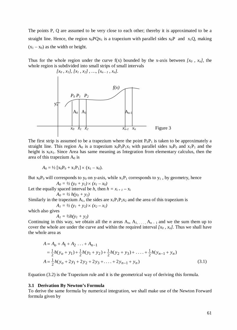
61

The points P, Q are assumed to be very close to each other; thereby it is approximated to be a

straight line. Hence, the region x0PQx1 is a trapezium with parallel sides x0P and x1Q, making

(x1 – x0) as the width or height.

Thus for the whole region under the curve f(x) bounded by the x-axis between [x0 , xn], the whole region is subdivided into small strips of small intervals [x0 , x1], [x1 , x2] , …, [xn – 1 , xn].

f(x)

P0 P1 P2

yo

A0 A1 An-1

x0 x1 x2 xn-1 xn Figure 3

The first strip is assumed to be a trapezium where the point P0P1 is taken to be approximately a straight line. This region A0 is a trapezium x0P0P1x1 with parallel sides x0P0 and x1P1 and the height is x0x1. Since Area has same meaning as Integration from elementary calculus, then the area of this trapezium A0 is

A0 = ½ [x0P0 + x1P1] × (x1 – x0).

But x0P0 will corresponds to y0 on y-axis, while x1P1 corresponds to y1 , by geometry, hence A0 = ½ (y0 + y1) × (x1 – x0) Let the equally spaced interval be h, then h = xi + 1 – xi A0 = ½ h(y0 + y1) Similarly in the trapezium A1, the sides are x1P1P2x2 and the area of this trapezium is A1 = ½ (y1 + y2) × (x2 – x1) which also gives A1 = ½h(y1 + y2) Continuing in this way, we obtain all the n areas Ao, A1, . . . , An – 1 and we the sum them up to cover the whole are under the curve and within the required interval [x0 , xn]. Thus we shall have the whole area as

)(....)()()(

...

121

3221

2121

121

121

nno

no

yyhyyhyyhyyh

AAAAA

++++++++=

+++=

−

−

)2....222( 132121

nno yyyyyyhA ++++++= − (3.1)

Equation (3.2) is the Trapezium rule and it is the geometrical way of deriving this formula. 3.1 Derivation By Newton’s Formula To derive the same formula by numerical integration, we shall make use of the Newton Forward formula given by

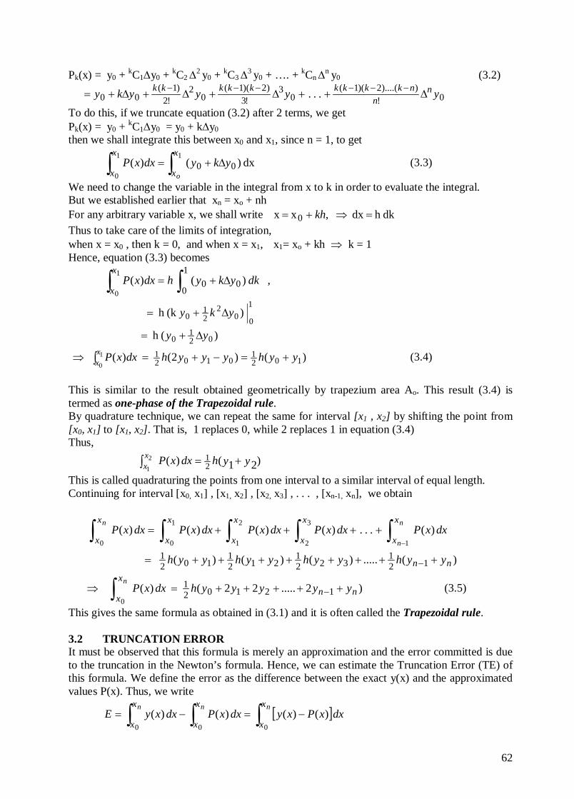
62

Pk(x) = y0 + kC1∆y0 + kC2 ∆2 y0 + kC3 ∆3 y0 + …. + kCn ∆n y0 (3.2) 0!

))....(2)(1(0

3!3

)2)(1(0

2!2

)1(00 ... yyyyky n

nnkkkkkkkkk ∆++∆+∆+∆+= −−−−−−

To do this, if we truncate equation (3.2) after 2 terms, we get Pk(x) = y0 + kC1∆y0 = y0 + k∆y0 then we shall integrate this between x0 and x1, since n = 1, to get

dx )( )(11

000∫∫ ∆+=

x

x

x

x oykydxxP (3.3)

We need to change the variable in the integral from x to k in order to evaluate the integral. But we established earlier that xn = xo + nh For any arbitrary variable x, we shall write dkh dx , x x 0 =⇒+= kh Thus to take care of the limits of integration, when x = x0 , then k = 0, and when x = x1, x1= xo + kh ⇒ k = 1 Hence, equation (3.3) becomes

, )( )(1

000

1

0∫∫ ∆+= dkykyhdxxP

x

x

1

002

21

0 ) (k h yky ∆+=

) (h 021

0 yy ∆+=

)()2( )( 1021

010211

0yyhyyyhdxxPx

x +=−+=⇒ ∫ (3.4)

This is similar to the result obtained geometrically by trapezium area Ao. This result (3.4) is termed as one-phase of the Trapezoidal rule. By quadrature technique, we can repeat the same for interval [x1 , x2] by shifting the point from [x0, x1] to [x1, x2]. That is, 1 replaces 0, while 2 replaces 1 in equation (3.4) Thus, )21()( 2

12

1yyhdxxPx

x +=∫

This is called quadraturing the points from one interval to a similar interval of equal length. Continuing for interval [x0, x1] , [x1, x2] , [x2, x3] , . . . , [xn-1, xn], we obtain

)(.....)()()(

)(...)()()()(

121

3221

2121

1021

1

3

2

2

1

1

00

nn

x

x

x

x

x

x

x

x

x

x

yyhyyhyyhyyh

dxxPdxxPdxxPdxxPdxxPn

n

n

++++++++=

++++=

−

∫∫∫∫∫−

)2.....22( )( 121021

0nn

x

xyyyyyhdxxP

n+++++=⇒ −∫ (3.5)

This gives the same formula as obtained in (3.1) and it is often called the Trapezoidal rule. 3.2 TRUNCATION ERROR It must be observed that this formula is merely an approximation and the error committed is due to the truncation in the Newton’s formula. Hence, we can estimate the Truncation Error (TE) of this formula. We define the error as the difference between the exact y(x) and the approximated values P(x). Thus, we write

[ ]∫∫∫ −=−=nnn x

x

x

x

x

xdxxPxydxxPdxxyE

000)()()()(

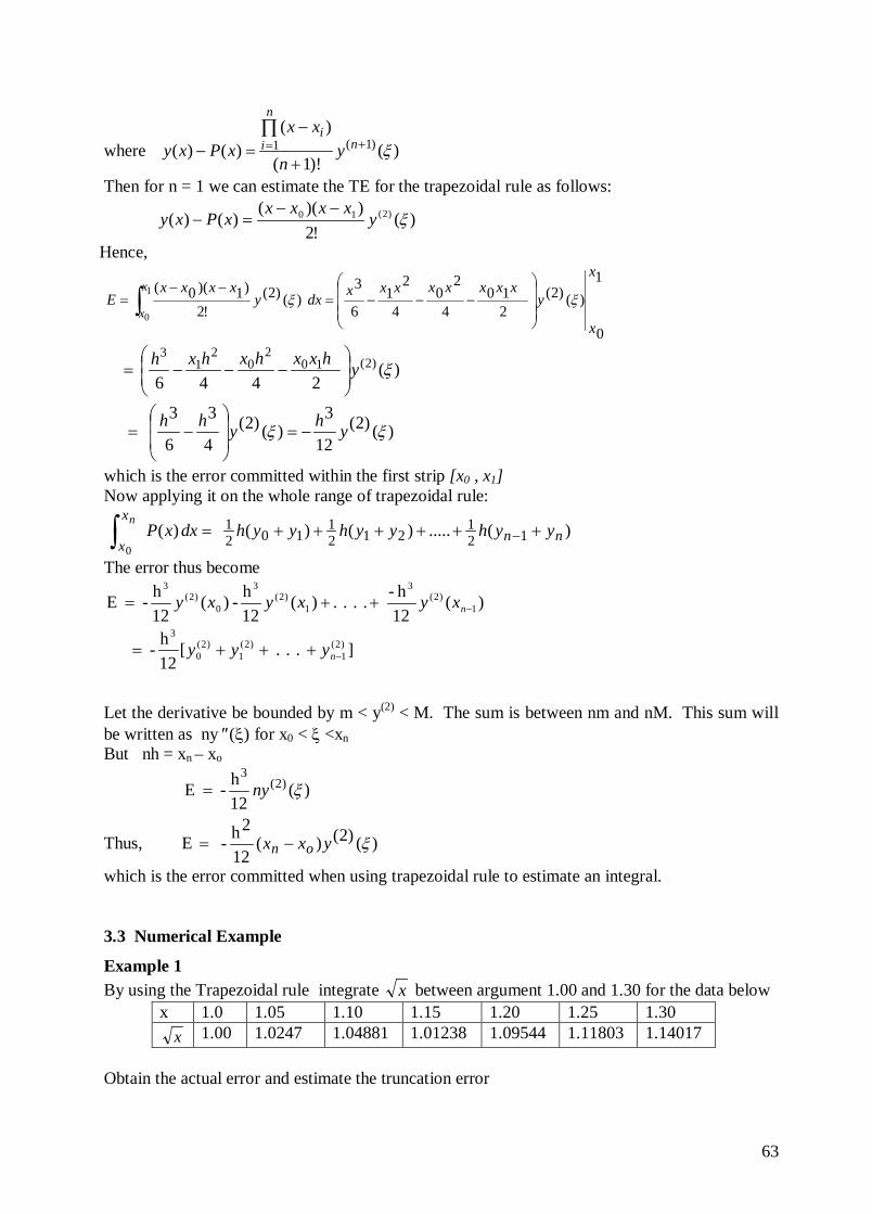
63

where )()!1(

)()()( )1(1 ξ+=

+

−=−∏

n

n

ii

yn

xxxPxy

Then for n = 1 we can estimate the TE for the trapezoidal rule as follows:

)(!2

))(()()( )2(10 ξy

xxxxxPxy

−−=−

Hence, 1

0

)()2(210

4

20

4

21

6

3)()2(

!2)1)(0(1

0

x

x

yxxxxxxxxdxy

xxxxE

x

xξξ

−−−=

−−= ∫

)(2446

)2(102

02

13

ξyhxxhxhxh

−−−=

)()2(12

3)()2(

4

3

6

3 ξξ yhyhh

−=

−=

which is the error committed within the first strip [x0 , x1] Now applying it on the whole range of trapezoidal rule:

)(.....)()( )( 121

2121

1021

0nn

x

xyyhyyhyyhdxxP

n++++++= −∫

The error thus become

)(12h- . . . .)(

12h-)(

12h- E 1

)2(3

1)2(

3

0)2(

3

−++= nxyxyxy

] . . . [12h- )2(

1)2(

1)2(

0

3

−+++= nyyy

Let the derivative be bounded by m < y(2) < M. The sum is between nm and nM. This sum will be written as ny ″(ξ) for x0 < ξ <xn But nh = xn – xo

)(12h- E )2(

3ξny=

Thus, E )()2()(12

2h- ξyxx on −=

which is the error committed when using trapezoidal rule to estimate an integral. 3.3 Numerical Example

Example 1 By using the Trapezoidal rule integrate x between argument 1.00 and 1.30 for the data below

x 1.0 1.05 1.10 1.15 1.20 1.25 1.30 x 1.00 1.0247 1.04881 1.01238 1.09544 1.11803 1.14017

Obtain the actual error and estimate the truncation error

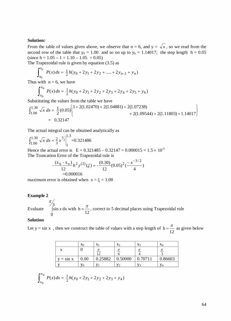
64

Solution: From the table of values given above, we observe that n = 6, and y = x , so we read from the second row of the table that y0 = 1.00 and so on up to y6 = 1.14017; the step length h = 0.05 (since h = 1.05 – 1 = 1.10 – 1.05 = 0.05) The Trapezoidal rule is given by equation (3.5) as

)2.....22( )( 121021

0nn

x

xyyyyyhdxxP

n+++++= −∫

Thus with n = 6, we have

)22222( )( 6543210216

0yyyyyyyhdxxP

x

x++++++=∫

Substituting the values from the table we have

14017.1)11803.1(2)09544.1(2

)07238.1(2)04881.1(2)02470.1(21)05.0(

21 30.1

00.1

++++++

=∫ dxx

= 0.32147 The actual integral can be obtained analytically as

3.1

13230.1

00.12

3 xdxx =∫ =0.321486

Hence the actual error is E = 0.321485 – 0.32147 = 0.000015 = 1.5 × 10-5

The Truncation Error of the Trapezoidal rule is

)4

()05.0(12

(0.30)-)(12

)x-(x-

2/32)2(2on

−−=

xyh ξ

=0.000016 maximum error is obtained when x = ξ = 1.00 Example 2

Evaluate ∫3

0dx sin

π

x with 12 h π= , correct to 5 decimal places using Trapezoidal rule

Solution

Let y = sin x , then we construct the table of values with a step length of 12 h π= as given below

)222( )( 43210214

0yyyyyhdxxP

x

x++++=∫

x0 x1 x2 x3 x4 x 0

12π

6π

4π

3π

y = sin x 0.00 0.25882 0.50000 0.70711 0.86603 y y0 y1 y2 y3 y4

65

( )[ ] 86603.0)70711.0(2)5.0(2)25882.0(20 sin 1221

0

3 ++++=∫ ππ

dxx

= 0.4971426 ≅ 0.49714 (correct to 5 decimal places) Analytically,

5.00coscoscos3

0dx sin 3

0

3=+−=−=∫ π

ππ

xx

Hence the absolute error is E = 0.5 – 0.49714 = 0.00286 = 2.86 × 10 -3

4.0 Conclusion The lesson has clearly shown that we need not know how to integrate a function before we can get an approximate value for such integral within a limiting boundary. We have also shown that the error committed can be compared with the actual value. This error is improved if the step length h is probably reduced. 5.0 Summary In this Unit we have learnt (i) how to derive the trapezoidal rule both in geometrical way and using the Newton Gregory

formula (ii) how to implement the trapezoidal rule to evaluate definite integrals (iii) that the error can be estimated by comparing with the analytical solution (iv) that the truncation error of the rule can be estimated 6.0 Tutor Marked Assignment

Evaluate ∫+

5

2dx

12

xwith

21 h = , correct to 5 decimal places using Trapezoidal rule

7.0 Further Reading and Other Resources

1. Conte S. D. and Boor de Carl Elementary Numerical Analysis an Algorithmic Approach 2nd ed. McGraw-Hill Tokyo.

2. Francis Scheid. (1989) Schaum’s Outlines Numerical Analysis 2nd ed. McGraw-Hill New York.

3. Okunuga, S. A., and Akanbi M, A., (2004). Computational Mathematics, First Course, WIM Pub. Lagos, Nigeria.

66

MODULE 4 UNIT 3 SIMPSON’S RULES 1.0 Introduction There are two popular Sampson’s rules. One is called the Simpson’s

31 - rule while the other is

the Simpson’s −83 rule. The Simpson’s rules are similarly useful in approximating definite

integrals. We shall discuss the Simpson’s 31 - rule in this Unit. Simpson’s

31 - rule is a technique

that uses 2 steps at a time to estimate the integral of P(x) as against single step used by Trapezoidal rule. So, the interval [x0, xn] is taken in two by two steps as [x0, x2] , [x2, x4] , [x4, x6] , . . . , [xn–2 , xn]. This idea will help us to derive a scheme that would be suitable for integration of various functions. 2.0 Objective At the end of this unit the learner must be able to

(i) derive the Simpson’s 31 - rule,

(ii) distinguish between Simpson’s rule and Trapezoidal rule, (iii) know where Simpson rule is applicable in terms of number of node points (iv) solve problems using the Simpson’s 1/3 rule

3.0 Derivation of Simpson’s

31 - Rule,

In order to develop a formula based on Simpson’s rule, we shall consider the integration of Newton Forward Formula (NFF) given in Unit 1 of this Module. Recall the NFF, we have Pk(x) = y0 + kC1∆y0 + kC2 ∆2 y0 + kC3 ∆3 y0 + …. + kCn ∆n y0 (3.1) 0!

))....(2)(1(0

3!3

)2)(1(0

2!2

)1(00 ... yyyyky n

nnkkkkkkkkk ∆++∆+∆+∆+= −−−−−−

If we integrate within the interval [x0, x2] and truncating after the third term, we shall obtain

∫∫ ∆+∆+= −2

0

2

0 )( )( 0

22

)1(00

x

x

kkx

xdxyykydxxP (3.2)

The integration has to be limited to 2x as n = 2 and this suggest the truncation also at ∆2.

Using the same technique employed earlier in Unit 2, to change the variable to k, we shall write

dkh dx , x x 0 =⇒+= kh Thus to take care of the limits of integration, we examine x0 and x2, so that when x = x0 , then k = 0, and when x = x2, x2= xo + kh ⇒ k = 2

Hence the integral (3.2) becomes

∫∫ ∆+∆+= −20 0

22

)1(00 )( )(2

0dkyykyhdxxP kkx

x

67

2

00

223

02

21

0 ))46

( (k h ykkyky ∆−+∆+=

)2 (2h 02

31

00 yyy ∆+∆+=

= h [2y0 + 2(y1 – y0) + 31 (y2 – 2y1 + y0)]

= 31 h [y0 + 4y1 + y2] (3.3)

which is a part or one phase of the Simpson’s 31 - rule.

By quadrature, we can shift to the next two steps, that is, [x2 , x4] to get the next integral as:

)4()( 432314

2yyyhdxxP

x

x++=∫

Continuing this interval up to (xn–2 , xn) and summing up all the phases, we have

∫∫∫∫−

+++=n

n

n

o

x

x

x

x

x

x

x

xdxxPdxxPdxxPdxxP

2

4

2

2

0)(...)()()(

)4(.....)4()4( )( 1231

43231

21031

0nnn

x

xyyyhyyyhyyyhdxxP

n+++++++++= −−∫

)42.....2424( )( 124321031

nnnnx

oxyyyyyyyyhdxxP ++++++++= −−∫ (3.4)

Equation (3.4) is known as the Simpson’s 31 - rule. It must be noted that due to the nature of this

formula, the formula will only be valid, if n is an even integer. That is, there must exist odd number of ordinates or collocating points within [x0 , xn]. Note that the formula has alternate coefficients of 4 and 2 starting with 4 and then followed by 2 and ending the second to the last term as 4 with exception of the first and the last term that have coefficient of 1. 3.1 Error Estimate of the Simpson’s 1/3 Rule The error committed while deriving the Simpson’s 1/3 rule is the error of truncation after the third term at ∆2. For this reason the truncation error can be estimated likewise as it was done for the trapezoidal Rule. Thus, if n = 2, the error committed on Simpson’s 3

1 - rule, which is the Truncation error is given by

E = )(180

a)-(b- )4(4 ξyh (3.5)

The reader is advised to verify this claim. 3.2 Determination of Step length Sometimes we may be given problems without specifying the step length h. However if the number of ordinates are given, which is the same as our n then we can determine the step length. To calculate the step length, the required formula is given by

1−

−=

mabh

68

where m is the number of ordinates given, a and b are the boundary of the integral. For example

given the integral ∫5

2)( dxxP and we are required to use 7 ordinates, then we recognize m = 7, a =

2 and b = 5, hence the step length h is obtained as

5.01725=

−−

=h

Hence our x0 = 2 then add 0.5 to subsequent xi until you get to b = 5. The last value must be the seventh ordinate which is x6. Thus we shall have x0 = 2, x1 = 2.5 , x2 = 3 x3 = 3.5, x4 = 4, x5 = 4.5, x6 = 5 3.3 Numerical Example Example 1 Integrate y= x within the limits 1.00 and 1.30 using the Simpson’s

31 - rule with 7 ordinates and

working with 5 decimal places. Hence estimate the error of this method. Solution: We first observe that this is the same question as the previous one in Trapezoidal rule. However in this case the table of values is not given hence we are to generate the table of values by computing the corresponding values of y for a given value of x. Further more we are to use 7 ordinates means that we need y0, y1, . . . . ,y6. , that is n = 6 (even), hence Simpson rule is applicable. Also since we are told to use 7 ordinates, we are required to determine the step length h. To do this, the given values are a = 1.00, b = 3.00 and m = 7 thus, the step length is calculated as

05.017

00.130.11

=−−

=−−

=m

abh ,

We then generate the table of values using calculator to find x for various values of x on the table.

Hence the table of values is similar to the example given in Unit 2 for this same question. By equation (3.4) the Simpson 1/3- rule is

)42.....2424( )( 124321031

0nnn

x

xyyyyyyyyhdxxP

n++++++++= −−∫

)4.2424( 654321031

3.1

1yyyyyyyhdxx ++++++=∫

Thus we evaluate the integral by simply substituting from our table above as

14017.1)11803.1(4)09544.1(2

)07238.1(4)04881.1(2)02470.1(41)05.0( 3

130.1

00.1

++++++

=∫ dxx

= 0.32149

x0 x1 x2 x3 x4 x5 x6 x 1.0 1.05 1.10 1.15 1.20 1.25 1.30 y= x 1.00 1.0247 1.04881 1.01238 1.09544 1.11803 1.14017 y y0 y1 y2 y3 y4 y5 y6

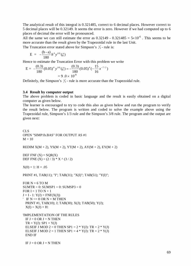
69

The analytical result of this integral is 0.321485, correct to 6 decimal places. However correct to 5 decimal places will be 0.32149. It seems the error is zero. However if we had computed up to 6 places of decimal the error will be pronounced. All the same we can still estimate the error as 0.32149 - 0.321485 = 5×10-6 . This seems to be more accurate than the result given by the Trapezoidal rule in the last Unit. The Truncation error stated above for Simpson’s 3

1 - rule is:

E = )(180

a)-(b- )4(4 ξyh

Hence to estimate the Truncation Error with this problem we write

E = )1615()05.0(

180(0.3)-)()05.0(

180(0.3)- 2/74)4(4 −−= xy ξ

= 9 .0 × 10-9 Definitely, the Simpson’s 3

1 - rule is more accurate than the Trapezoidal rule.

3.4 Result by computer output The above problem is coded in basic language and the result is easily obtained on a digital computer as given below. The learner is encouraged to try to code this also as given below and run the program to verify the result below. The program is written and coded to solve the example above using the Trapezoidal rule, Simpson’s 1/3 rule and the Simpson’s 3/8 rule. The program and the output are given next: CLS OPEN "SIMP1b.BAS" FOR OUTPUT AS #1 M = 10 REDIM X(M + 2), YS(M + 2), YT(M + 2), AY(M + 2), EY(M + 2) DEF FNF (X) = SQR(X) DEF FNE (X) = (2 / 3) * X ^ (3 / 2) X(0) = 1: H = .05 PRINT #1, TAB(11); "I"; TAB(31); "X(I)"; TAB(51); "Y(I)"; FOR N = 6 TO M SUMTR = 0: SUMSP1 = 0: SUMSP3 = 0 FOR I = 1 TO N + 1 J = I - 1: Y(J) = FNF(X(J)) ' IF N <= 8 OR N = M THEN PRINT #1, TAB(10); J; TAB(30); X(J); TAB(50); Y(J); X(I) = X(J) + H: 'IMPLEMENTATION OF THE RULES IF J = 0 OR J = N THEN TR = Y(J): SP1 = Y(J) ELSEIF J MOD 2 = 0 THEN SP1 = 2 * Y(J): TR = 2 * Y(J) ELSEIF J MOD 2 = 1 THEN SP1 = 4 * Y(J): TR = 2 * Y(J) END IF IF J = 0 OR J = N THEN

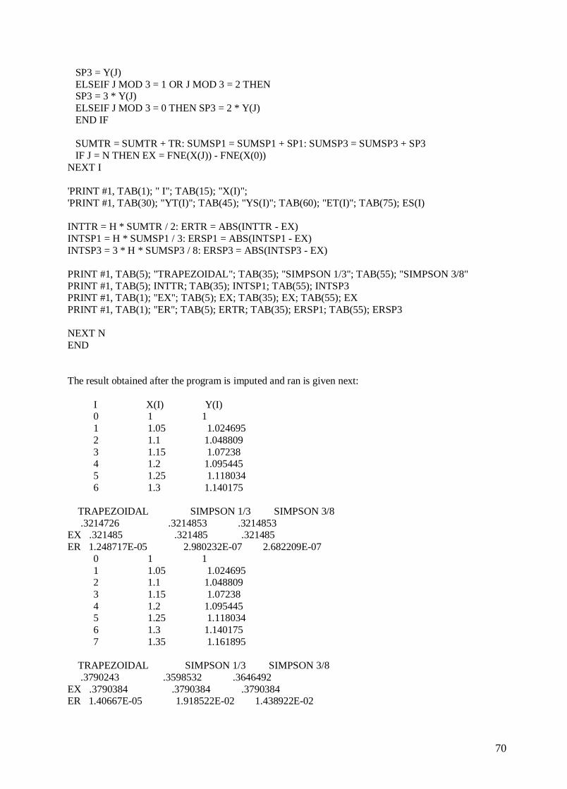
70

SP3 = Y(J) ELSEIF J MOD 3 = 1 OR J MOD 3 = 2 THEN SP3 = 3 * Y(J) ELSEIF J MOD 3 = 0 THEN SP3 = 2 * Y(J) END IF SUMTR = SUMTR + TR: SUMSP1 = SUMSP1 + SP1: SUMSP3 = SUMSP3 + SP3 IF J = N THEN EX = FNE(X(J)) - FNE(X(0)) NEXT I 'PRINT #1, TAB(1); " I"; TAB(15); "X(I)"; 'PRINT #1, TAB(30); "YT(I)"; TAB(45); "YS(I)"; TAB(60); "ET(I)"; TAB(75); ES(I) INTTR = H * SUMTR / 2: ERTR = ABS(INTTR - EX) INTSP1 = H * SUMSP1 / 3: ERSP1 = ABS(INTSP1 - EX) INTSP3 = 3 * H * SUMSP3 / 8: ERSP3 = ABS(INTSP3 - EX) PRINT #1, TAB(5); "TRAPEZOIDAL"; TAB(35); "SIMPSON 1/3"; TAB(55); "SIMPSON 3/8" PRINT #1, TAB(5); INTTR; TAB(35); INTSP1; TAB(55); INTSP3 PRINT #1, TAB(1); "EX"; TAB(5); EX; TAB(35); EX; TAB(55); EX PRINT #1, TAB(1); "ER"; TAB(5); ERTR; TAB(35); ERSP1; TAB(55); ERSP3 NEXT N END The result obtained after the program is imputed and ran is given next: I X(I) Y(I) 0 1 1 1 1.05 1.024695 2 1.1 1.048809 3 1.15 1.07238 4 1.2 1.095445 5 1.25 1.118034 6 1.3 1.140175 TRAPEZOIDAL SIMPSON 1/3 SIMPSON 3/8 .3214726 .3214853 .3214853 EX .321485 .321485 .321485 ER 1.248717E-05 2.980232E-07 2.682209E-07 0 1 1 1 1.05 1.024695 2 1.1 1.048809 3 1.15 1.07238 4 1.2 1.095445 5 1.25 1.118034 6 1.3 1.140175 7 1.35 1.161895 TRAPEZOIDAL SIMPSON 1/3 SIMPSON 3/8 .3790243 .3598532 .3646492 EX .3790384 .3790384 .3790384 ER 1.40667E-05 1.918522E-02 1.438922E-02

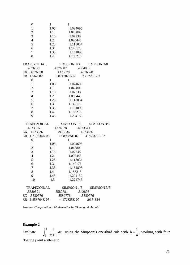
71

0 1 1 1 1.05 1.024695 2 1.1 1.048809 3 1.15 1.07238 4 1.2 1.095445 5 1.25 1.118034 6 1.3 1.140175 7 1.35 1.161895 8 1.4 1.183216 TRAPEZOIDAL SIMPSON 1/3 SIMPSON 3/8 .4376521 .4376682 .4304055 EX .4376678 .4376678 .4376678 ER 1.567602 3.874302E-07 7.26226E-03 0 1 1 1 1.05 1.024695 2 1.1 1.048809 3 1.15 1.07238 4 1.2 1.095445 5 1.25 1.118034 6 1.3 1.140175 7 1.35 1.161895 8 1.4 1.183216 9 1.45 1.204159 TRAPEZOIDAL SIMPSON 1/3 SIMPSON 3/8 .4973365 .4774578 .4973541 EX .4973536 .4973536 .4973536 ER 1.713634E-05 1.989585E-02 4.768372E-07 0 1 1 1 1.05 1.024695 2 1.1 1.048809 3 1.15 1.07238 4 1.2 1.095445 5 1.25 1.118034 6 1.3 1.140175 7 1.35 1.161895 8 1.4 1.183216 9 1.45 1.204159 10 1.5 1.224745 TRAPEZOIDAL SIMPSON 1/3 SIMPSON 3/8 .5580591 .5580781 .542896 EX .5580776 .5580776 .5580776 ER 1.853704E-05 4.172325E-07 .0151816 Source: Computational Mathematics by Okunuga & Akanbi Example 2

Evaluate dxx∫ +

3

1 11 using the Simpson’s one-third rule with

41 h = , working with four

floating point arithmetic

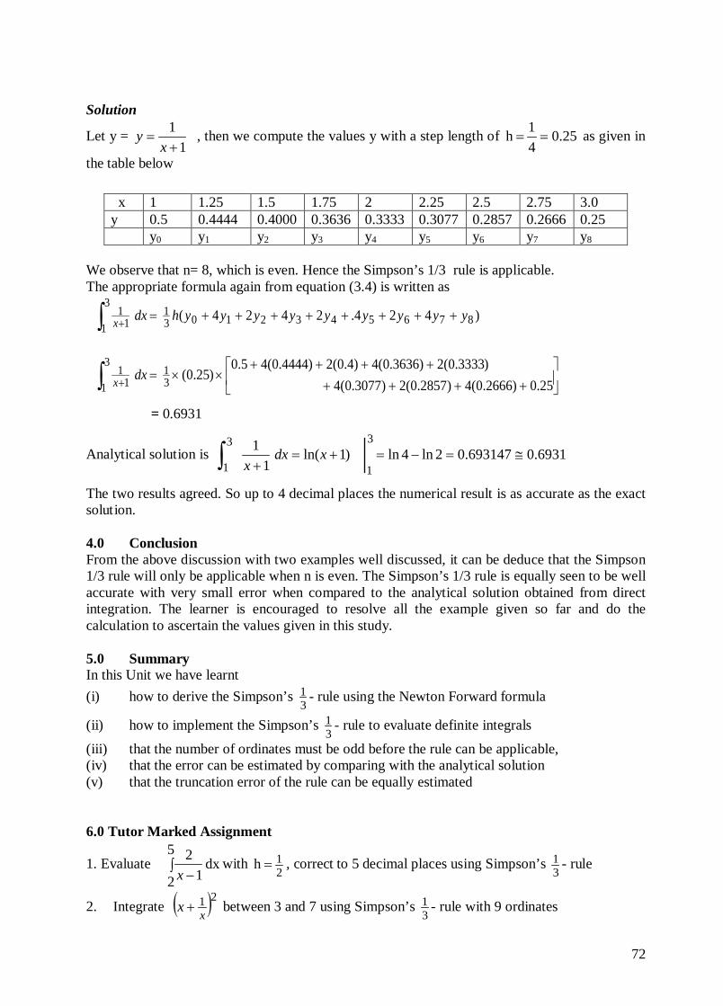
72

Solution

Let y = 1

1+

=x

y , then we compute the values y with a step length of 25.041 h == as given in

the table below

We observe that n= 8, which is even. Hence the Simpson’s 1/3 rule is applicable. The appropriate formula again from equation (3.4) is written as

)424.2424( 87654321031

3

1 11 yyyyyyyyyhdxx ++++++++=∫ +

25.0)2666.0(4)2857.0(2)3077.0(4

)3333.0(2)3636.0(4)4.0(2)4444.0(45.0)25.0( 3

13

1 11

++++

++++××=∫ + dxx

= 0.6931

Analytical solution is 6931.0693147.02ln4ln)1ln(1

1 3

1

3

1≅=−=+=

+∫ xdxx

The two results agreed. So up to 4 decimal places the numerical result is as accurate as the exact solution. 4.0 Conclusion From the above discussion with two examples well discussed, it can be deduce that the Simpson 1/3 rule will only be applicable when n is even. The Simpson’s 1/3 rule is equally seen to be well accurate with very small error when compared to the analytical solution obtained from direct integration. The learner is encouraged to resolve all the example given so far and do the calculation to ascertain the values given in this study. 5.0 Summary In this Unit we have learnt (i) how to derive the Simpson’s

31 - rule using the Newton Forward formula

(ii) how to implement the Simpson’s 31 - rule to evaluate definite integrals

(iii) that the number of ordinates must be odd before the rule can be applicable, (iv) that the error can be estimated by comparing with the analytical solution (v) that the truncation error of the rule can be equally estimated 6.0 Tutor Marked Assignment

1. Evaluate ∫−

5

2dx

12

xwith

21 h = , correct to 5 decimal places using Simpson’s

31 - rule

2. Integrate ( )21xx + between 3 and 7 using Simpson’s

31 - rule with 9 ordinates

x 1 1.25 1.5 1.75 2 2.25 2.5 2.75 3.0 y 0.5 0.4444 0.4000 0.3636 0.3333 0.3077 0.2857 0.2666 0.25 y0 y1 y2 y3 y4 y5 y6 y7 y8

73

7.0 Further Reading and Other Resources

1. Atkinson K.E. (1978): An Introduction to Numerical Analysis, 2nd Edition, John Wiley & Sons, N.Y

2. Conte S. D. and Boor de Carl Elementary Numerical Analysis an Algorithmic Approach 2nd ed. McGraw-Hill Tokyo.

3. Francis Scheid. (1989) Schaum’s Outlines Numerical Analysis 2nd ed. McGraw-Hill New York.

4. Kandassamy P., Thilagarathy K., & Gunevathi K. (1997) : Numerical Methods, S. Chand & Co Ltd, New Delhi, India

5. Okunuga, S. A., and Akanbi M, A., (2004). Computational Mathematics, First Course, WIM Pub. Lagos, Nigeria.

74

MODULE 4 UNIT 4 NEWTON-COTES FORMULAS 1.0 Introduction

Apart from Trapezoidal rule and Simpson 31 rule, we also have the Simpson 8

3 rule. Beyond this we have other formulas based on the same Newton Forward Formula (NFF) with higher n. For

example we recall that Trapezoidal rule use interval [x0, x1], Simpson 31 rule use [x0, x2], and

Simpson 83 rule will use [x0, x3] to obtain a one-phase of its formula. The formulas that use [x0,

xn], where n is greater than 3, are called Newton-Cotes formula. Invariably, Newton–Cotes formula generalizes all the rules including the ones earlier discussed. We shall in this unit consider the remaining formulas for approximating definite integrals. 2.0 Objective At the end of this unit the learner must be able to

(v) derive the Simpson 83 - rule,

(vi) distinguish between the Newton – Cotes formulas (vii) Simpson’s rule and Trapezoidal rule, (viii) know where Simpson rule is applicable in terms of number of node points

(ix) solve problems using the Simpson’s 31 rule

3.0 Simpson 83 Rule

The Simpson 83 formula follows from the Simpson 3

1 rule. The complete derivation will not be given in this unit, but a sketch of it. However the technique is virtually the same as the ones earlier proved, since the derivation is from the same Newton Forward Formula. The learner is advised to verify some of the formulas stated in this Unit.

Suppose the Newton Forward Formula (NFF) is truncated after the fourth term or after the third forward difference (that is for n = 3) and integration is carried out within [x0 , x3], we can write

( )∫∫ ∆+∆+∆+= −−−3

0

3

0

)( 03

!3)2)(1(

02

2)1(

00

x

x

kkkkkx

xdxyyykydxxP (3.1)

Changing the variables from x to k and integrating, we shall obtain

)3 3 (h )( 3210833

0yyyydxxP

x

x+++=∫ (3.2)

This is known as a one-phase of the Simpson 3/8 – rule. When quadrature principle is applied, we obtain the Simpson 3/8 – rule finally as

( )nnnx

xyyyyyyyyyydxxP

n++++++++++= −−∫ 1265432108

3 3 3 ...23 3 23 3 h )(0

(3.3)

The coefficients are also systematic. The inner coefficients are 3, 3, 2, while the first and last term have 1 as the coefficient. The number of ordinates can only be 4, 7, 10, and so on When we have 4 ordinates we have the formula

)3 3 (h )( 3210833

0yyyydxxP

x

x+++=∫ (3.4)

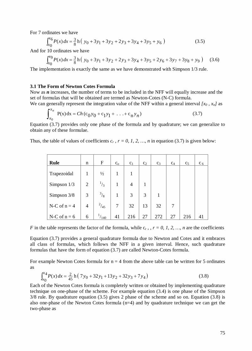
75

For 7 ordinates we have

( )6543210836

03 3 23 3 h )( yyyyyyydxxP

xx

++++++=∫ (3.5)

And for 10 ordinates we have

( )9876543210839

03 323 3 23 3 h )( yyyyyyyyyydxxP

xx

+++++++++=∫ (3.6)

The implementation is exactly the same as we have demonstrated with Simpson 1/3 rule. 3.1 The Form of Newton Cotes Formula Now as n increases, the number of terms to be included in the NFF will equally increase and the set of formulas that will be obtained are termed as Newton-Cotes (N-C) formula. We can generally represent the integration value of the NFF within a general interval [x0 , xn] as

)nc . . . 11c 00(c dxP(x)0

nyyyChnx

x+++=∫ (3.7)

Equation (3.7) provides only one phase of the formula and by quadrature; we can generalize to obtain any of these formulae.

Thus, the table of values of coefficients cr , r = 0, 1, 2, …, n in equation (3.7) is given below:

Rule n F co c1 c2 c3 c4 c5 c 6

Trapezoidal

Simpson 1/3

Simpson 3/8

N-C of n = 4

N-C of n = 6

1

2

3

4

6

½

1/3

3/8

2/45

1/140

1

1

1

7

41

1

4

3

32

216

1

3

13

27

1

32

272

7

27

216

41

F in the table represents the factor of the formula, while cr , , r = 0, 1, 2, …, n are the coefficients

Equation (3.7) provides a general quadrature formula due to Newton and Cotes and it embraces all class of formulas, which follows the NFF in a given interval. Hence, such quadrature formulas that have the form of equation (3.7) are called Newton-Cotes formula. For example Newton Cotes formula for n = 4 from the above table can be written for 5 ordinates as

( )432104524

07 3213 32 7 h )( yyyyydxxP

xx

++++=∫ (3.8)

Each of the Newton Cotes formula is completely written or obtained by implementing quadrature technique on one-phase of the scheme. For example equation (3.4) is one phase of the Simpson 3/8 rule. By quadrature equation (3.5) gives 2 phase of the scheme and so on. Equation (3.8) is also one-phase of the Newton Cotes formula (n=4) and by quadrature technique we can get the two-phase as

76

( )8765432104524

07 3213 32 14 3213 32 7 h )( yyyyyyyyydxxP

xx

++++++++=∫

Similar procedure is applicable to other Newton-Cotes formula. Self Assessment Test Write from the table the next possible Newton-Cotes formula for n = 4 4.0 Conclusion We have seen that there are several other formulas that can be used for approximate integration. The simplest of them is the Trapezoidal rule without any restriction on the number of ordinates. The other formulas or rules however have some restriction on the number of ordinates that must be prescribed before each of them could be used. 5.0 Summary In this Unit we have learnt (i) how to derive the Simpson’s 3/8- rule using the Newton Forward formula (ii) the structure of the Newton-Cotes formulas (iii) that the implementation of any of the Newton Cotes formulas is similar to Simpson’s

31 -

rule for evaluating definite integrals (iv) that the number of ordinates is important before a particular rule can be applied, (v) that the formulas are obtained by quadraturing the one-phase of the formula. 6.0 Tutor Marked Assignment

1. Evaluate ∫−

5

2dx

12

xwith

21 h = , correct to 5 decimal places using Simpson 3/8- rule. Compare

your result with the analytical solution 2. Integrate 1+x between 3 and 7, correct to 5 decimal places, using (i) Simpson’s 3/8- rule with 7 ordinates (ii) Newton Cotes formula (n=4) with 9 ordinates Compare your result with the analytical solution and deduce which of the two is more accurate

3 Evaluate ∫5

1dx log xe correct to 6 decimal places with 9 ordinates

Use (i) Trapezoidal rule (ii) Simpson 1/3-rule (iii) Newton Cotes formula (n=4)

For evaluation. Obtain the actual error, which of these is most accurate? 7.0 Further Reading and Other Resources

1. Atkinson K.E. (1978): An Introduction to Numerical Analysis, 2nd Edition, John Wiley & Sons, N.Y

2. Conte S. D. and Boor de Carl Elementary Numerical Analysis an Algorithmic Approach 2nd ed. McGraw-Hill Tokyo.

3. Francis Scheid. (1989) Schaum’s Outlines Numerical Analysis 2nd ed. McGraw-Hill New York.

4. Okunuga, S. A., and Akanbi M, A., (2004). Computational Mathematics, First Course, WIM Pub. Lagos, Nigeria.

77

MODULE 5

BOUNDARY VALUE PROBLEMS

UNIT 1: INTRODUCTION TO BOUNDARY VALUE PROBLEMS 1.0 Introduction What is a Boundary Value Problem? This is a kind of problem that is related to differential equations. A differential equation can be an Ordinary Differential Equation (ODE) or a Partial Differential Equation (PDE). However, an ODE can be classified into two, viz: (i.) Initial Value Problem (IVP) and (ii) Boundary Value Problem (BVP). These two classes of differential equations are of great importance and so their numerical solutions are equally studied under Numerical Analysis. We shall give the definition of the two. 2.0 Objective At the end of this lesson, the learner would have been able to

(i) distinguish between Initial Value Problem and Boundary Value Problem (ii) derive finite difference scheme for solving BVP (iii) solve BVP using a finite difference scheme

3.0 Distinction Between IVP and BVP There is a distinction between an Initial Value Problem and a Boundary Value Problem. As the name goes, one is prescribed with an initial condition while the other is prescribed with boundary conditions. For a better understanding we shall define both ordinary differential equation and partial differential equation before distinguish between IVP and BVP. We hereby give the following definitions.

Definition 1 A differential equation involving ordinary derivatives (or total derivatives) with respect to a single independent variable is called an ordinary differential equation. Some examples of ODEs are given below.

2

2 2 0d y dyx ydxdx

− + =

2

3 7dy dyy xdx dx

− = −

2 cosdy xy xdx

− =

Definition 2 A differential equation involving partial derivatives of one or more dependent variables with respect to more than one independent variable is called a Partial Differential Equation (PDE) Some examples of PDEs are given below.

(i) 2vsv

tv

=∂∂

+∂∂

78

(ii) 02

2

2

2=

∂∂

+∂∂

yu

xu

Definition 3: (Initial Value Problem) An Initial Value Problem (IVP) can be defined as an Ordinary Differential Equation with a condition specified at an initial point.

For example: oo yxycbydxdya ==+ )(, (3.1)

Where xo and yo are initial point of the equation. This example is simple enough as this involves only a single first order ODE. It is possible to have a system of first order ODEs with initial conditions all through for each of the equations. However we may have some other differential equations with some conditions specified either at the derivative or at the boundary of the problem being defined. This leads to the next definition. Definition 4: (Boundary Value Problem) A Boundary Value Problem (BVP) is a differential equation either an Ordinary Differential Equation (ODE) or Partial Differential Equation (PDE) with at least two specified conditions at the boundary points. The boundary points often will contain an initial point and the other at the end point of the problem. The two serve as the boundary to the problem. For example for an Ordinary Differential Equation a simple example of a BVP will be:

nono xxxxyxydcydxdyb

dx

yda ≤≤===++ ,)(,)(,2

2βα (3.2)

The above equation is a second order differential equation which is solvable for the specified range of values of x. Two conditions are specified at the extremes or the boundaries. That is the conditions are given at x = x0 and x = xn. Example of a BVP involving a PDE will be given later when discussing the methods of solving Partial Differential Equations. There are several numerical methods available today for solving first order ODEs with an initial condition. This is a course on its own as the subject is wide, though not so tasking. However, the focus of this course and Module is to expatiate on methods of solving BVPs. Hence, we shall in limit our discussion to the numerical methods for solving the BVPs of ordinary differential equations. 3.1 SOLUTION OF BVP OF ODE The numerical solution of a second order Ordinary Differential Equation usually will involve solving system of equations. To do this, some approximations are put in place to replace the derivative function involved in the given differential equation. Suppose we are to solve the differential equation (3.2) using a numerical method, Two popular methods among other methods of solving this equation are either by Finite Difference Method (FDM) or by Shooting method. We shall in this unit discuss the Finite Difference Method for solving equation (3.2). Consider the Taylor series expansion of the function y(x+h) where h is regarded as the step length to be used in the problem. Then we shall obtain

)()()()()( 3!22

hOxyxyhxyhxy h +′′+′+=+ (3.3)

79

where O(h3) is called error of order 3 representing the truncation error of where the expansion is terminated. We can obtain a first derivative approximation from this expansion by writing

)()()()(

)()()()()(

2

3!22

hOxyhxyhxy

hOxyxyhxyhxy h

+′=−+

+′′+′=−+

Dividing through by h we obtain

)()()()( hOh

xyhxyxy +−+

=′ (3.4)

Which shows that for small step length h, the error in approximating )(xy′ is proportional to h. Furthermore if we expand the function y(x – h) we equally get

)()()()()( 3!22

hOxyxyhxyhxy h −′′+′−=− (3.5)

We can also obtain a first derivative approximation from this expansion as

)()()()( hOh

hxyxyxy +−−

=′ (3.6)

Equations (3.4) and (3.6) are approximations to )(xy′ which can be used to replace the function as it may be required. Equation (3.4) is the forward difference representation while equation (3.6) is the backward difference representation. Now suppose we take the difference of equations (3.3) and (3.5) we shall obtain

)()(2)()( 3hxyhhxyhxy +′=−−+ This reduces to

)()()()( 2hOh

hxyhxyxy +−−+

=′ (3.7)

Equation (3.7) is a central difference approximation to )(xy′ . It would be observed that the error in the last equation is smaller than that of the two equations (3.4) or (3.6), since for small h, h2 will be smaller than h. On the other hand if we add equations (3.3) and (3.5) we shall obtain

)()()2()(2)()( 4!22

hOxyxyhxyhxy h +′′+=−++

⇒ )()()()(2)( 42 hOxyhhxyxyhxy +′′=−+−+ Divide through by h2 we obtain

)()()(2)()( 22

hOh

hxyxyhxyxy +−+−+

=′′ (3.8)

This is a standard representation for the second derivative. Thus equations (3.4) and (3.8) can be substituted into equation (3.2) to obtain a numerical scheme for solving that equation. Recall the differential equation (3.2)

ccydxdyb

dx

yda =++2

2

Substituting (3.4) and (3.8) we have

dxcyh

xyhxybh

hxyxyhxya =+

−+

+

−+−+ )()()()()(2)(2

80

evaluating at x = xn, we observe that 11)()()( ++ ==+=+ nnn yxyhxyhxy Also 11)()()( −− ==−=− nnn yxyhxyhxy hence, we obtain

dxcyh

xyhxyb

h

hxyxyhxya n

nnnnn =+

−++

−+−+)(

)()()()(2)(2

dych

yyb

h

yyya n

nnnnn =+

−+

+− +−+ 12

11 2

( ) ( ) 22111 2 dhychyybhyyya nnnnnn =+−++− +−+ (3.9)

On the other hand, we can use the central difference to replace the first derivative to get

dych

yyb

h

yyya n

nnnnn =+

−+

+− −+−+2

2 112

11

( ) ( ) 22112

111 2 dhychyybhyyya nnnnnn =+−++− −+−+ (3.10)

Equations (3.9) and (3.10) are numerical schemes that can be used to solve equation (3.2). Either of these will yield the desire result with slight difference in accuracy. On applying the boundary conditions in (3.2) and writing the resulting equations for n = 1, 2, . . . , k-1, we obtain a system of equations with equal number of unknowns. The above shall be illustrated by the next example. 3.2 Numerical Examples

Example 1 Solve the boundary value problem (BVP) 22 2)1( xyyxyx =−′+′′+ (3.11) Satisfying the boundary conditions y(0) = 1 and y(1) = 0 You may use a step length of 0.25. Solution To solve this problem we can apply the approximation of the derivatives to the given equation (11), we then obtain

( ) 2112

1122

22

1 nnnn

nnnn

n xyh

yyx

h

yyyx =−

−+

+−+ −+−+

Since 41=h it implies that the range of x is divided into four parts by 5 node points

Thus x0 = 0 and x4 = 1 (that is : x1 = 0.25 x2 = 0.5 x3 = 0.75 ) The boundary condition y(0) = 1 and y(1) = 0 simply transform to y0 = 1 and y4 = 0 Since n = 0 will be invalid as we will not be able to evaluate y-1 then the reasonable thing to do as in the theory above is to substitute n = 1,2,3,4. Hence, we obtain With n = 1, the formula above becomes

h

0 0.25 0.5 0.75 1

81

( )( ) ( )

211

41

212

41

1221 2

22

1 xyyy

xyyy

x oo =−

−+

+−

+

( )( )

( ) ( ) ( )241

141

241

241

12241

2

12121 =−

−

+

+−

+ yyyy

( )( ) ( )

161

12121617 11216 =−−++− yyyy

255560288 12 −=− yy (i)

Also for n = 2, we have

( )( ) ( )

222

41

1322

41

12322 2

22

1 xyyy

xyyy

x =−

−+

+−

+

( )( )

( ) ( ) ( )221

241

1321

241

123221

22

21 =−

−+

+−

+ y

yyyyy

( )( ) ( )41

21312345 2216 =−−++− yyyyyy

17216488 123 =+− yyy (ii) And for n = 3, we have

( )( )

( ) ( ) ( )243

341

2443

241

234243

22

21 =−

−

+

+−

+ yyyyyy

9352784448 234 =+− yyy 9352784 23 −=− yy (iii)

since y4 = 0. Thus we have a system of 3 equations in three unknowns y1 , y2 , y3. The matrix form of these three equations from (i), (ii), (iii), is written as:

−

−=

−−

−

91255

784352088164720288560

321

yyy

On solving, correct to four decimal places, we obtain

=

=

1465.03519.06363.0

545447991

53571885

599984381783

321

yyy

82

Thus the values corresponding to y1 , y2 , y3 are the results of the differential equation at points x1 , x2 , x3. 4.0 Conclusion We have seen that the finite difference scheme is systematic and dynamic in producing solution to BVP. The resulting technique led to system of linear equations which can be solved by any available methods used for solving such system. The learner can also check other texts for other method of solving BVP in ODE, such as the shooting method earlier mentioned. 5.0 Summary In this Unit we have learnt

(i) distinction between BVP and IVP (ii) how to derive the Finite Difference scheme for solving BVP (iii) how to implement the Finite Difference Method on a BVP.

6.0 Tutor Marked Assignment Solve the boundary value problem xyyxyx 22 =−′+′′ , satisfying the boundary conditions y(0) = 1 and y(1) = 0, use a step length h = 0.25. 7.0 Further Reading and Other Resources

1. Francis Scheid. (1989) Schaum’s Outlines Numerical Analysis 2nd ed. McGraw-Hill New York.

2. Kandassamy P., Thilagarathy K., & Gunevathi K. (1997) : Numerical Methods, S. Chand & Co Ltd, New Delhi, India

3. Turner P. R. (1994) Numerical Analysis Macmillan College Work Out Series Malaysia

83

MODULE 5: UNIT 2: BOUNDARY VALUE PROBLEMS INVOLVING PARTIAL

DIFFERENTIAL EQUATIONS 1.0 Introduction

As earlier stated, a Boundary Value Problem (BVP) could be a Partial Differential Equation (PDE) with two specified points at the initial point and at the boundary point. In scientific computing many problems are governed by non linear differential equation which requires a solution in a region R subject to exact condition on the boundary. Unlike the BVP involving an ODE, most BVPs usually occur from problems involving rate of change with respect to two or more independent variables. Such problems lead to PDEs. The two dimensional second order Partial Differential Equation is generally of the form

02

22

2

2=++

∂∂

+∂∂

+∂

∂+

∂∂∂

+∂

∂ gfuyue

xud

y

ucyxub

x

ua (1.1)

where u is a function of two variables x and y, that is, u = u(x, y) The solution of this equation subject to prescribed conditions is generally obtained through some analytical methods by separating the variables x and y. However, the numerical solution of equation (1.1) can be obtained either by the finite difference method or the finite element method. 2.0 Objective At the end of this lesson, the learner would have been able to

(i.) define a second order PDE (ii.) define a Boundary Value Problem (BVP) involving a partial differential equation (iii.) classify various types of PDEs (iv.) classify types of boundary conditions among PDEs (v.) derive finite difference schemes for PDEs.

3.0 Types Of Partial Differential Equations A number of mathematical models describing the physical system are the special cases of general second order PDE

0),,,,()(2

22

2

2=

∂∂

∂∂

−∂

∂+

∂∂∂

+∂

∂=

yu

xuuyxH

y

uCyxuB

x

uAuL (3.1)

Or 0),,,,()( =−++= yxyyxyxx uuuyxHCuBuAuuL The following definitions are given with respect to equation (3.1). Equation (3.1) is said to be semi-linear, if A, B and C are functions of independent variables x and y only. If A, B and C are functions of x, y, u, ux and uy, then (3.1) is termed to be quasi-linear. However, when A, B and C are functions of x and y and H is a linear function of u, ux and uy, then (3.1) is said to be linear. Hence, the most general second order linear PDE in two independent variables can be written as

0),(),(),(),(),(),(),( =++++++ yxGuyxFuyxEuyxDuyxCuyxBuyxA yxyyxyxx (3.2) When G(x, y) = 0, then equation (3.2) is known as a linear homogenous second order PDE. A solution of equation (3.1) or (3.2) will be of the form

u = u(x, y)

84

Which represents a surface in (x, y, u) space called the integral surface. If on the integral surface, there exist curves across which the derivatives uxx, uyy and uxy are discontinuous or indeterminate then the curves are called “characteristics”. For this, we assume the solution of equation (3.1) is passing through a curve C whose parametric equations are x = x(s) , y = y(s) and u = u(s) (3.3) Furthermore, let each point (x, y, u) of curve C and the partial derivates ux and uy be known since the solution is of the form (3.3) at each point of x, y of curve C. 3.1 Classification of Partial Differential Equations

Thus there are two families of curve which can be obtained from equation (3.1) along which the second order derivatives will not be determined in a definite or finite manner. There are called characteristics curves which are classified according to the following conditions. If

B2 – 4AC > 0 , then we have real and distinct roots B2 – 4AC < 0, then we have imaginary roots B2 – 4AC = 0 , then we have real and coincidence or equal roots

Hence, the Partial Differential Equation (3.1) or (3.2) is said to be: Parabolic, if B2 – 4AC = 0 It is Elliptic if B2 –4 AC < 0 and it is Hyperbolic, if B2 – 4AC > 0

Few examples are given below to illustrate these classifications. Examples 1. The wave equation is given by

2

2

2

2

x

u

t

u

∂

∂=

∂

∂

This equation is a Hyperbolic equation, since A = 1, B = 0 , C = -1 so that, B2 – 4AC = 4 > 0 2. The heat flow equation is given by

2

2

x

utu

∂

∂=

∂∂

Comparison with equation (3.1), we note that: A = 0, B = 0 , C = -1 so that B2 – 4AC = 0, Hence the heat flow equation is a Parabolic equation. 3. The Laplace equation is also given by

02

2

2

2=

∂

∂+

∂

∂

y

u

x

u

Comparison with equation (3.1), shows that: A = 1, B = 0 , C = 1 so that B2 – 4AC = – 4 < 0. Thus the Laplace equation is an Elliptic equation. 3.2 Classification of Boundary Conditions for PDE The parabolic and hyperbolic types of equations are either IVP or initial BVP whereas the elliptic equation is always a BVP. There are three types of boundary conditions. These are given below as follows:

i) Dirichlet Conditions

85

Here the function (say u(x,y)) is prescribed along the boundary. If the function takes on zero value along the boundary, the conditions is called homogenous dirchlet condition otherwise it is called inhomogenous dirichlet boundary conditions.

ii) The Neumann Boundary Condition

Here the derivative of the function is specified along the boundary. We may also have homogenous or inhomogenous boundary conditions

iii) Mixed Boundary Conditions Here the function and its derivatives are prescribed along the boundary. We may also have homogenous and inhomogenous conditions.

3.3 Finite Difference Scheme Most PDEs are solved numerically by Finite Difference Method (FDM), although another known method is the Finite Element Method (FEM). Hence, there is the need to develop schemes of finite differences for derivatives of some functions. In ODE of the second order which was discussed earlier, the function y is a function of a single variable x. The treatment of the finte difference method was easier. However a similar technique and analogy will be employed for the development of the finite difference schemes (FDS) of a second order PDE. The difference now is u being a function of two variables x and y. In this regard, finite difference schemes or methods required that the (x, y) region of the problem to be examined be divided into smaller regions by rectilinear grid, mesh or lattice of discrete points with co-ordinates (xi, yj) given by

yjyy

xixx

oj

oiδ

δ+=+=

This shows that each axis is divided into set of equal intervals by node points. Usually we shall represent kyhx == δδ , as our step lengths in x and y directions respectively. Hence,

rkyyrhxx nrnnrn +=+= ++ , Consider a function u(x, y) of two variables, with an increment xδ in x yield

),(),( yhxuyxxu +=+δ If this is expanded by Taylor series, we shall obtain

...),(!2

),(),(),( 2

22−

∂

∂+

∂∂

+=+x

yxuhx

yxuhyxuyhxu (i)

Similarly ),( yxxu δ− , the expansion yield

...),(!2

),(),(

),(),(

2

22−

∂

∂+

∂∂

−=

−=−

xyxuh

xyxuhyxu

yhxuyxxu δ

((ii)

Other expansions with increments on y give:

...),(!2

),(),(

),(),(

2

22+

∂

∂+

∂∂

+=

+=+

y

yxuky

yxukyxu

kyxuyyxu δ

(iii)

86

...),(!2

),(),(

),(),(

2

22−

∂

∂+

∂∂

−=

−=−

y

yxuky

yxukyxu

kyxuyyxu δ

(iv)

Truncating equation (i) at second term yields,

xx huhOyxhuyxuyhxu ≅+=−+ )(),(),(),( 2

hyxuyhxuux),(),( −+

= (3.4)

at point (i, j) we have

hyxuyhxu

yxu jijijix

),(),(),(

−+=

hyxuyxu

xyxu jijiji ),(),(),( 1 −

=∂

∂ +

This is then written for easy handling as:

or h

uuu jiji

x,,1 −

= + (3.5)

Similarly from (iii) by following the same procedure, we get

k

uuu

yu jiji

y,, 1 −==

∂∂ + (3.6)

Equations (3.5) and (3.6) are forward difference approximation of ux and uy respectively. Similarly, truncating at third time we shall obtain the second derivative approximation. This can be achieved by taking the sum of equations (i) and (ii), to get

2

22),(2),(),(

x

uhyxuyhxuyhxu∂

∂+=−++

2

22

11 ),(2),(),(x

uhyxuyxuyxu jijiji∂

∂+=+ −+

This simplified to

211

2

2 ,,2,

h

uuuu

x

u jijijixx

−+ +−==

∂

∂ (3.7)

Also adding equations (iii) and (iv), we obtain a similar result as

211

2

2 ,,2,

k

uuuu

y

u jijijiyy

−+ +−==

∂

∂ (3.8)

Equations (3.7) and (3.8) are the finite difference approximation for the second derivatives uxx and uyy. They are sometimes called the second central difference approximations. These approximations are often used to develop the finite difference schemes which are tools for solving BVPs numerically. 4.0 Conclusion We have seen that the subject of BVP is wide. Partial differential equations with boundary conditions differ depending on the type of boundary conditions. This will invariably affect the scheme which will be developed for its solution. We remark here that the basic differentiation formula as we have in analysis is the same used here for the development of the finite differences for the partial derivatives.

87

5.0 Summary In this Unit we have learnt

(i) The definition for various types of PDEs, (ii) About types of boundary conditions (iii) how to derive the finite differences for first and second partial derivatives.

6.0 Tutor Marked Assignment

Write a finite difference for yxu∂∂

∂2

7.0 Further Reading and Other Resources 1. Conte S. D. and Boor de Carl Elementary Numerical Analysis an Algorithmic Approach

2nd ed. McGraw-Hill Tokyo. 2. Francis Scheid. (1989) Schaum’s Outlines Numerical Analysis 2nd ed. McGraw-Hill New

York. 3. Kandassamy P., Thilagarathy K., & Gunevathi K. (1997) : Numerical Methods, S. Chand

& Co Ltd, New Delhi, India 4. Leadermann Walter (1981) (Ed.): Handbook of Applicable Mathematics, Vol 3,

Numerical Analysis, John Wiley, N.Y.

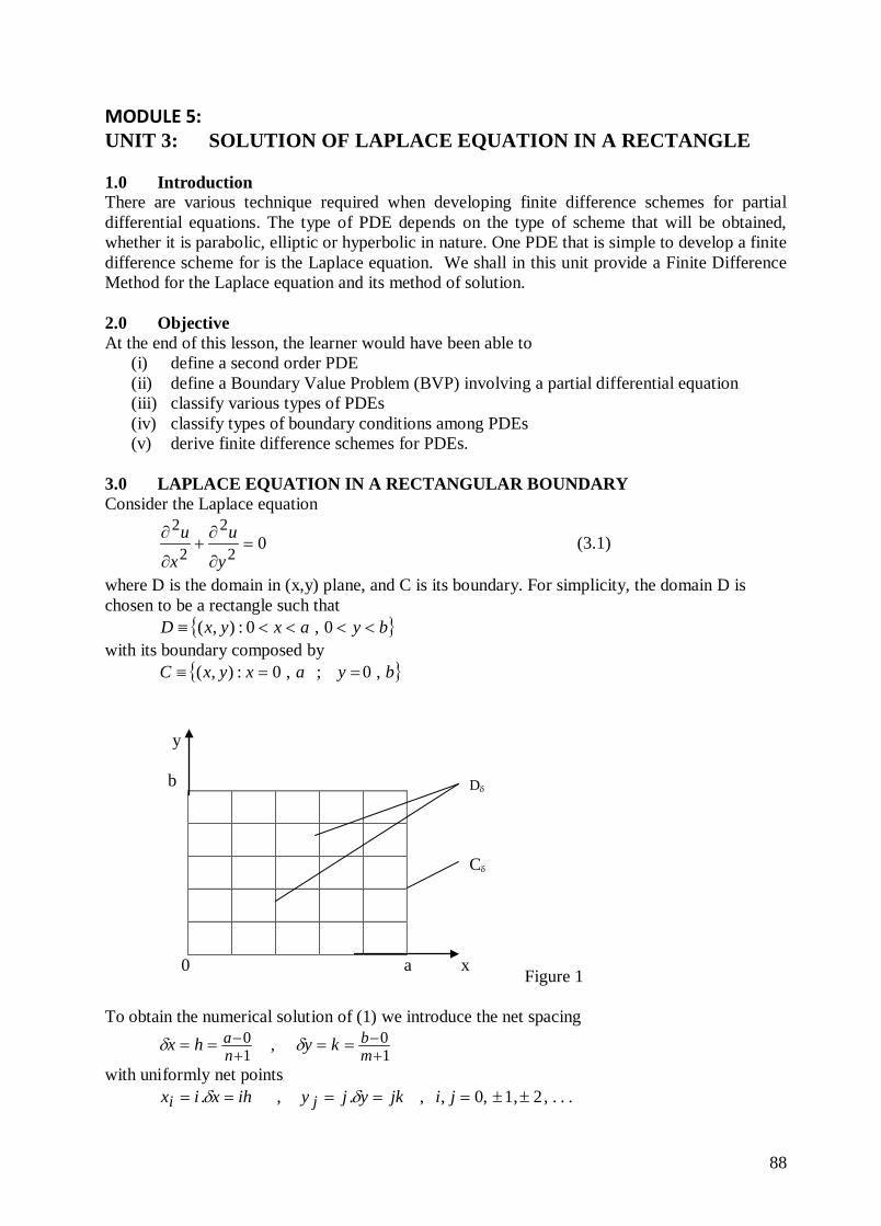
88

MODULE 5: UNIT 3: SOLUTION OF LAPLACE EQUATION IN A RECTANGLE 1.0 Introduction There are various technique required when developing finite difference schemes for partial differential equations. The type of PDE depends on the type of scheme that will be obtained, whether it is parabolic, elliptic or hyperbolic in nature. One PDE that is simple to develop a finite difference scheme for is the Laplace equation. We shall in this unit provide a Finite Difference Method for the Laplace equation and its method of solution. 2.0 Objective At the end of this lesson, the learner would have been able to

(i) define a second order PDE (ii) define a Boundary Value Problem (BVP) involving a partial differential equation (iii) classify various types of PDEs (iv) classify types of boundary conditions among PDEs (v) derive finite difference schemes for PDEs.

3.0 LAPLACE EQUATION IN A RECTANGULAR BOUNDARY Consider the Laplace equation

02

2

2

2=

∂

∂+

∂

∂

y

u

x

u (3.1)

where D is the domain in (x,y) plane, and C is its boundary. For simplicity, the domain D is chosen to be a rectangle such that { }byaxyxD <<<<≡ 0,0:),( with its boundary composed by

{ }byaxyxC ,0;,0:),( ==≡ Figure 1 To obtain the numerical solution of (1) we introduce the net spacing

10

10 ,

+−

+− ==== m

bna kyhx δδ

with uniformly net points ...,2,1,0,,.,. ±±===== jijkyjyihxix ji δδ

y b

0 a x

Dδ

Cδ

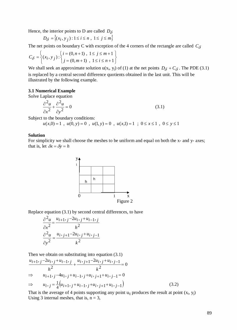
89

Hence, the interior points to D are called δD { }mjniyxD ji ≤≤≤≤= 1,1:),(δ

The net points on boundary C with exception of the 4 corners of the rectangle are called δC

+≤≤+=+≤≤+=

=11,)1,0(11,)1,0(

:),(nimj

mjniyxC jiδ

We shall seek an approximate solution u(xi, yj) of (1) at the net points δδ CD + . The PDE (3.1) is replaced by a central second difference quotients obtained in the last unit. This will be illustrated by the following example. 3.1 Numerical Example Solve Laplace equation

02

2

2

2=

∂

∂+

∂

∂

y

u

x

u (3.1)

Subject to the boundary conditions: 10,10;1)1,(,0),1(,0),0(,1)0,( ≤≤≤≤==== yxxuyuyuxu Solution For simplicity we shall choose the meshes to be uniform and equal on both the x- and y- axes; that is, let hyx == δδ Replace equation (3.1) by second central differences, to have

211

2

2 ,,2,

h

uuu

x

u jijiji −+ +−=

∂

∂

211

2

2 ,,2,

k

uuu

y

u jijiji −+ +−=

∂

∂

Then we obtain on substituting into equation (3.1)

0,,2,,,2,

211

211 =

+−+

+− −+−+

k

uuu

h

uuu jijijijijiji

⇒ 0,,,,4, 1111 =+++− −+−+ jijijijiji uuuuu

⇒ ( )111141 ,,,,, −+−+ +++= jijijijiji uuuuu (3.2)

That is the average of 4 points supporting any point uij produces the result at point (xi, yj) Using 3 internal meshes, that is, n = 3,

y 1

h h

0 1 x

Figure 2

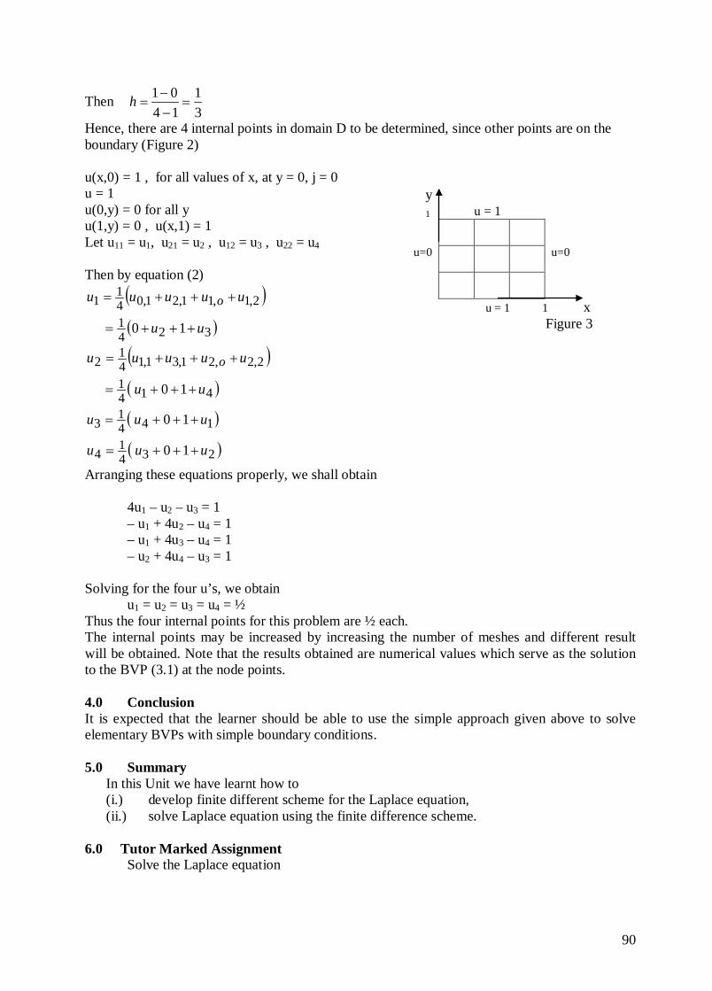
90

Then 31

1401=

−−

=h

Hence, there are 4 internal points in domain D to be determined, since other points are on the boundary (Figure 2) u(x,0) = 1 , for all values of x, at y = 0, j = 0 u = 1 u(0,y) = 0 for all y u(1,y) = 0 , u(x,1) = 1 Let u11 = u1, u21 = u2 , u12 = u3 , u22 = u4 Then by equation (2)

( )( )324

1

2,1,11,21,041

1

10 uu

uuuuu o

+++=

+++=

( )( )414

1

2,2,21,31,141

2

10 uu

uuuuu o

+++=

+++=

( )1441

3 10 uuu +++=

( )2341

4 10 uuu +++=

Arranging these equations properly, we shall obtain

4u1 – u2 – u3 = 1 – u1 + 4u2 – u4 = 1 – u1 + 4u3 – u4 = 1 – u2 + 4u4 – u3 = 1

Solving for the four u’s, we obtain

u1 = u2 = u3 = u4 = ½ Thus the four internal points for this problem are ½ each. The internal points may be increased by increasing the number of meshes and different result will be obtained. Note that the results obtained are numerical values which serve as the solution to the BVP (3.1) at the node points. 4.0 Conclusion It is expected that the learner should be able to use the simple approach given above to solve elementary BVPs with simple boundary conditions. 5.0 Summary

In this Unit we have learnt how to (i.) develop finite different scheme for the Laplace equation, (ii.) solve Laplace equation using the finite difference scheme.

6.0 Tutor Marked Assignment

Solve the Laplace equation

y 1 u = 1

u = 1 1 x

Figure 3

u=0 u=0

91

02

2

2

2=

∂

∂+

∂

∂

y

u

x

u

Subject to the boundary conditions: 10,10;1)1,(,0),1(,0),0(,1)0,( ≤≤≤≤==== yxxuyuyuxu Use h = ¼ on both axes 7.0 Further Reading and Other Resources

1. Francis Scheid. (1989) Schaum’s Outlines Numerical Analysis 2nd ed. McGraw-Hill New York.

2. Henrici P. (1982): Essential of Numerical Analysis, Wiley, N.Y 3. Kandassamy P., Thilagarathy K., & Gunevathi K. (1997) : Numerical Methods, S. Chand

& Co Ltd, New Delhi, India 4. Leadermann Walter (1981) (Ed.): Handbook of Applicable Mathematics, Vol 3,

Numerical Analysis, John Wiley, N.Y. 5. Turner P. R. (1994) Numerical Analysis Macmillan College Work Out Series Malaysia