Embed Size (px)
Citation preview

NATIONAL OPEN UNIVERSITY OF NIGERIA
SCHOOL OF ARTS AND SOCIAL SCIENCES
COURSE CODE: ECO 253
COURSE TITLE: STATISTICS FOR ECONOMISTS
NATIONAL OPEN UNIVERSITY OF NIGERIA
STATISTICS FOR ECONOMISTS
ECO 253
SCHOOL OF ARTS AND SOCIAL SCIENCES
COURSE GUIDE
Course Developer:
Okojie, Daniel Esene E-mail: [email protected]
School of Postgraduate Studies (SPGS)
University of Lagos (UNILAG) Akoka,
Yaba, Lagos State
Nigeria.
Course Content Editor Dr Ibrahim Bakare
STATISTICS FOR ECONOMISTS ECO 253
NOUN 2
COURSE CONTENT:
Main Introduction
Course Outline
Aims
Course Objectives
Working through the Course
Course Materials Study Units
Textbooks and Reference Resources Assignment Folder
Presentation Plan
Assessment
Tutor-Marked Assignments (TMAs)
Concluding Examination and Grading
Marking Scheme
Overview Making the Most of this Course
Tutors and Tutorials
Summary
STATISTICS FOR ECONOMISTS ECO 253
NOUN 3
Main Introduction
The topics covered in this course include: The Normal, Binomial and Poisson
Distributions, Estimate Theory, Test of Statistical hypothesis including t, f and chi-
square tests analysis of least square method, correlation and Regression analyses.
Others are elementary sampling theory and design of experiments, non-parametric
methods, introduction to the central limit theory (CLT) and the law of large numbers.
The course focuses progressively on elementary understanding of distribution
functions and other inferential statistical techniques. The course focuses on practical
issues involved in the substantive interpretation of economic data using sampling,
estimation, hypothesis testing, correlation, and regression. For this reason, empirical
case studies that apply the techniques to real-life data are stressed and discussed
throughout the course, and students are required to perform several statistical
analyses on their own.
The course is a very useful material to you in your academic pursuit and helps to
further broaden your understanding of the role of statistics in the study of economics.
This course is developed to guide you on what statistics for economists’ entails, what
course materials in line with a course learning structure you will be using. The
learning structure suggests some general guidelines for a time frame required of you
on each unit in order to achieve the course aims and objectives effectively.
Course Outline
ECO 253 is made up of twenty five units spread across twelve lectures weeks and
covering areas such as Normal, Binomial and Poisson Distributions, correlation and
Regression analysis, Estimation Theory which will introduce you to its different
discrete nature and models. Also to be outlined is test of statistical hypothesis using
t, f and chi-square. Others are elementary sampling theory and design of experiments,
non-parametric methods, introduction to the central limit theory (CLT) and the law of large
numbers.
Aims
The aims in this course are to give you thorough understanding and an appreciative
importance of statistics in the study of economics in you becoming an Economist.
That it is almost impossible to find a problem which does not require a general use of
statistical data. Important phenomena in all branches of economics can be described,
compared and correlated with the help of Statistics with examples to demonstrate its
applications in business and economics. There will be a strong emphasis on the
concepts and application of tests analysis methods, random variables, distributions,
sampling theory, statistical inference, correlation and regression.
Others are statistical inference techniques such as estimation and significance testing
are important in the fitting and interpretation of econometric models. Correlation and
STATISTICS FOR ECONOMISTS ECO 253
NOUN 4
regression analysis are essential tools for measuring relationships between variables
and for prediction
Course Objectives
To achieve the aims set above in addition with the overall slated course objectives,
each unit would also have its specific objectives. The unit objectives are included at
the beginning of a unit; you should read them before you start working through the
unit. You may want to refer to them during your study of the unit to check on your
progress. You should always look at the unit objectives after completing a unit. In
this way, you can be certain you have done what was necessary of you by the unit.
The course objectives are set below for you to achieve the aims of the course. On
successful conclusion of the course, you should be able to:
Identify and gather economic data
Do basic data manipulation and hypothesis testing State statistical estimation of economic relationships
Apply correlation and regression analyses models to data
Understand non-parametric methods, elementary sampling theory and design
of experiments
Discuss in an introductory manner central limit theory and the law of large numbers
Solve problems that could lead you to using some standard statistical
software.
Working through the Course
To successfully complete this course, you are required to read the study units,
referenced books and other materials on the course.
Each unit contains self-assessment exercises called Student Assessment Exercises
(SAE). At some points in the course, you will be required to submit assignments for
assessment purposes. At the end of the course there is a final examination. This course
should take about twelve weeks to complete and some components of the course are
outlined under the course material subsection.
Course Material
The major component of the course, what you have to do and how you should allocate
your time to each unit in order to complete the course successfully and on time are as
follow:
1. Course guide
2. Study unit
3. Textbook
4. Assignment file 5. Presentation schedule
Study Unit
STATISTICS FOR ECONOMISTS ECO 253
NOUN 5
In this course, there are five modules that are subdivided into 20 units which should be
studied diligently and with utmost care.
Module 1: Probability and Statistic Distribution Functions Unit 1: Bernoulli Distribution
Unit 2: Binomial Distribution
Unit 3: Normal Distribution
Unit 4 Poisson Distribution
Module 2: Statistical Hypothesis Test Unit 5: T- test
Unit 6: F- test Unit 7: Chi square test
Unit 8: ANOVA
Unit 9: Parametric and Non-Parametric test Methods
Module 3: Correlation and Regression Coefficient Analyses Unit 10: Pearson’s Correlation Coefficient
Unit 11: Spearman’s Rank Correlation Coefficient Unit 12: Methods of Curve and Eye Fitting of Scattered Plot and the Least
Square Regression Line Unit 13: Forecasting in Regression
Module 4: Introduction to the Central Limit Theory (CLT)
Unit 14: Central Limit Theorems for Independent Sequences
Unit 15: Central Limit Theorems for dependent Processes Unit 16: Relation to the law of large numbers
Unit 17: Extensions to the theorem and Beyond the Classical Framework
Module 5: Index Numbers and Introduction to Research Methods in Social Sciences
Unit 18: Index Number
Unit 19: Statistical Data
Unit 20: Sample and Sampling Techniques
Here module 1 (units 1-4) presents you with the common probability distribution
functions as a general background on the course, statistics for economists; the
discreteness of Bernoulli, Binomial and Poisson distributions and the continuous
natures of Normal distribution are shown.
Module 2 (units 5-9) explains some statistical hypothesis tests; the t-test, f-test, chi
square test, analysis of variance (ANOVA), parametric and non-parametric test methods are all introduced. Their usage, significance, samples comparison and
application for economists are also explained.
Correlation and Regression Coefficient Analyses are contained in module 3 (unit 10-
13). This module explores Pearson’s Correlation Coefficient, Spearman’s Rank
STATISTICS FOR ECONOMISTS ECO 253
NOUN 6
Correlation Coefficient, the Least Square Regression Line and Forecasting in
Regression. The module 4 (unit 14-17) covers detail description of an introduction to
central limit theory (CLT). CL theorems for independent sequences, dependent
processes and the relation to law of large numbers brought to the students’ knowledge
here. Also, extensions to the theorem and beyond the classical framework are
presented in units 17 of module 4. While basic concepts and notation of elementary
Index Numbers and Introduction to Research Methods in Social Sciences are in units 18-20
of module 5. This module 5 (units 18-20) has present in it: Index Number, Statistical
Data and Sample & Sampling Techniques.
.
Each study unit will take at least two hours, and it include the introduction, objective,
main content, examples, In-Text Questions (ITQ) and their solutions, self-assessment
exercise, conclusion, summary and reference. Other areas border on the Tutor-Marked Assessment (TMA) questions. Some of the ITQ and self-assessment exercise will
require you brainstorming and solving with some of your colleagues. You are advised
to do so in order to comprehend and get acquainted with how important statistics is in
making the most of economics.
There are also statistical materials, textbooks under the reference and other (on-line
and off-line) resources for further reading. They are meant to give you additional
information whenever you avail yourself of such opportunity. You are required to
study the materials; practise the ITQ and self-assessment exercise and TMA questions
for greater and in-depth understanding of the course. By doing so, the stated learning
objectives of the course would have been achieved.
Textbook and References For additional reading and more detailed information about the course, the following
reference texts and materials are recommended:
Adebayo O. A., (2006). Understanding Statistics: Lagos, 5th
Edition Lagos Nigeria
JAS Publisher.
Spiegel, Murray R. and Walpole, Ronald E., (1992). Theory and Problems of
Statistics op. cit: Introduction to Statistic. 2nd
Ed. Collier Macmillan International Editions.
Walpole R. E., Richard Lerson and Morris Marx (1995), An Introduction to
Mathematical Statistics and Its Applications, 5th
Edition New York: John Wiley
& Sons. Inc.
Dowling Edward T., (2001). Mathematical Economics 2nd
Edition; Schaum Outline
Series.
Esan E. O. and Okafor R. O., Basic Statistical Methods, Lagos, Nigeria. JAS
Publishers. ISBN – 978 – 33180 – 0 – 4

STATISTICS FOR ECONOMISTS ECO 253
NOUN 7
Assignment Folder There are assignments on this course and you are expected to do all of them by
following the schedule prescribed for them in terms of when to attempt them and
submit same for grading by your lecturer. The marks you obtain for these assignments
will count toward the final mark you obtain for this course. Further information on
assignments will be found in the Assignment File itself and later in this Course Guide
in the section on Assessment.
There are five assignments in this course. These five course assignments will cover:
Assignment 1 - All TMAs’ question in Units 1 – 4 (Module 1)
Assignment 2 - All TMAs' question in Units 5 – 9 (Module 2)
Assignment 3 - All TMAs' question in Units 10 – 13 (Module 3)
Assignment 4 - All TMAs' question in Units 14 – 17 (Module 4)
Assignment 5 - All TMAs' question in Units 18 – 20 (Module 5)
Presentation Plan The presentation plan included in your course materials gives you the important dates
for this year for the completion of tutor-marking assignments and attending tutorials.
Remember, you are required to submit all your assignments by due date. You should
guide against falling behind in your work.
Assessment There are two types of assessments this course. First is the tutor-marked assignment
and second, would be a written examination.
In attempting the assignments, you are expected to apply information, knowledge and
techniques gathered during the course. The assignments must be submitted to your
tutor/lecturer for formal Assessment in accordance with the deadlines stated in the
Presentation Schedule and the Assignments File. The work you submit to your tutor
for assessment will count for 30 % of your total course mark.
At the end of the course, you will need to sit for a final written examination of three
hours' duration. This examination will also count for 70% of your total course mark.
Tutor-Marked Assignments (TMAs) There are five tutor-marked assignments in this course. You will submit all the
assignments. You are encouraged to work all the questions thoroughly. The TMAs
constitute 30% of the total score.
Assignment questions for the units in this course are contained in the Assignment File.
You will be able to complete your assignments from the information and materials
contained in your textbooks, reading and study units. However, it is desirable that you
demonstrate that you have read, solved a lot problems relating to each module topic
and researched more widely than the required minimum. You should use other
references to have a broad viewpoint of the subject and also to give you a deeper
understanding of the subject.

STATISTICS FOR ECONOMISTS ECO 253
NOUN 8
When you have completed each assignment, send it, together with a TMA form, to your
tutor. Make sure that each assignment reaches your tutor on or before the
deadline given in the Presentation File. If for any reason, you cannot complete your
work on time, contact your tutor before the assignment is due to discuss the possibility
of an extension. Extensions will not be granted after the due date unless there are
exceptional conditions.
Unit Unit Title
Course Guide
Probability and Statistic Distribution Functions
Week’s
Activity Assessment (end of unit)
1 Bernoulli Distribution Week 1
2 Binomial Distribution Week 2
Normal Distribution 3
Poisson Distribution 4
Statistical Hypothesis Test
Week 3 Week 4 Assignment 1
5 T-test Week 5
6 F-test Week 6
7 Chi square test Week 7
8 ANOVA Week 8
9 Parametric and Non-Parametric test methods Week 9 Assignment 2
Correlation and Regression Coefficient Analysis
10 Pearson’s Correlation Coefficient Week 10
11 Spearman’s Rank Correlation Coefficient Week 11
12 The Least Square Regression Line Week12
13 Forecasting in Regression Week 13 Assignment 3
Introduction to the Central Limit Theory (CLT)
14 Central Limit Theorems for Independent Sequences Week 14
15 Central Limit Theorems for dependent Processes Week 15
16 Relation to the law of large numbers Week 16
17 Extensions to the theorem & Beyond the classical framework Week 17 Assignment 4
Index Numbers and Introduction to Research Methods in Social Sciences
Index Number
18
Statistical Data
19
Week 18
Week 19
20 Sample and Sampling Techniques Week 20 Assignment 5
Total 20 Weeks
Examination
Concluding Examination and Grading

STATISTICS FOR ECONOMISTS ECO 253
NOUN 9
The concluding and final examination on the course will be of three hours' duration
and has a value of 70% of the total course grade. The examination will consist of
questions which reflect the types of self-assessment practice exercises and tutor-
marked problems you have previously encountered. All areas of the course will be
assessed
You are advised to use the time between finishing the last unit and sitting for the
examination to revise the entire course materials. You might find it useful to review
your In-Text Questions (ITQ) and self-assessment exercises, tutor-marked
assignments and comments on them before the examination. The final examination
covers the entire course outline.
Marking Scheme The table presented below indicate the total marks (100%) allocation.
Assessment Marks
Assignment (Best three assignment out of the five marked) 30% Final Examination 70%
Total 100%
Overview The table presented below indicate the units, number of weeks and assignments to be taken by you to successfully complete the course, Statistics for Economists (ECO
203).
Making the Most of this Course
An advantage of the distance learning is that the study units replace the university
lecturer. You can read and work through specially designed study materials at your
own tempo and at a time and place that goes well with you.
Consider doing it yourself in solving and providing solutions to statistical problems in the lecture instead of listening and copying solution being provided by a lecturer. In
the same way that a lecturer might set you some practice exercises and ITQ to do, the
study units tell you when to solve problems and read your books or other material, and
when to embark on discussion with your colleagues. Just as a lecturer might give you
an in-class exercise, your study units provides exercises for you to do at appropriate
points.
Each of the study units follows a common format. The first item is an introduction to
the subject matter of the unit and how a particular unit is integrated with the other
units and the course as a whole. Next is a set of learning objectives. These objectives
let you know what you should be able to do by the time you have completed the unit.
You should use these objectives to guide your study. When you have finished the unit
you must go back and check whether you have achieved the objectives. If you make a
habit of doing this you will significantly improve your chances of passing the course
and getting the best grade.
The main body of the unit guides you through the required understanding from other
sources. This will usually be either from your set books or from a readings section.

STATISTICS FOR ECONOMISTS ECO 253
NOUN 10
Some units require you to undertake practical overview of real life statistical events.
You will be directed when you need to embark on discussion and guided through the
tasks you must do.
The purpose of the practical overview of real life statistical events is in twofold. First,
it will enhance your understanding of the material in the unit. Second, it will give you
practical experience and skills to evaluate economic arguments, and understand the
roles of statistics in guiding current economic problems, calculations, analysis,
solutions and debates outside your studies. In any event, most of the critical thinking
skills you will develop during studying are applicable in normal working practice, so
it is important that you encounter them during your studies.
Self-assessments are interspersed throughout the units, and answers are given at the
ends of the units. Working through these tests will help you to achieve the objectives
of the unit and prepare you for the assignments and the examination. You should do
each self-assessment exercises as you come to it in the study unit. Also, ensure to
master some major statistical theorems and models during the course of studying the
material.
The following is a practical strategy for working through the course. If you run into
any trouble, consult your tutor. Remember that your tutor's job is to help you. When
you need help, don't hesitate to call and ask your tutor to provide it.
1. Read this Course Guide thoroughly.
2. Organize a study schedule. Refer to the `Course overview' for more details.
Note the time you are expected to spend on each unit and how the assignments
relate to the units. Important information, e.g. details of your tutorials, and the date of the first day of the semester is available from study centre. You need to gather together all this information in one place, such as your dairy or a wall
calendar. Whatever method you choose to use, you should decide on and write
in your own dates for working breach unit.
3. Once you have created your own study schedule, do everything you can to stick
to it. The major reason that students fail is that they get behind with their
course work. If you get into difficulties with your schedule, please let your
tutor know before it is too late for help.
4. Turn to Unit 1 and read the introduction and the objectives for the unit.
5. Assemble the study materials. Information about what you need for a unit is
given in the `Overview' at the beginning of each unit. You will also need both
the study unit you are working on and one of your set books on your desk at the same time.
6. Work through the unit. The content of the unit itself has been arranged to
provide a sequence for you to follow. As you work through the unit you will be
instructed to read sections from your set books or other articles. Use the unit to
guide your reading.
7. Up-to-date course information will be continuously delivered to you at the
study centre.
8. Work before the relevant due date (about 4 weeks before due dates), get the
Assignment File for the next required assignment. Keep in mind that you will
STATISTICS FOR ECONOMISTS ECO 253
NOUN 11
learn a lot by doing the assignments carefully. They have been designed to help
you meet the objectives of the course and, therefore, will help you pass the
exam. Submit all assignments no later than the due date.
9. Review the objectives for each study unit to confirm that you have achieved
them. If you feel unsure about any of the objectives, review the study material
or consult your tutor.
10. When you are confident that you have achieved a unit's objectives, you can
then start on the next unit. Proceed unit by unit through the course and try to
pace your study so that you keep yourself on schedule. 11. When you have submitted an assignment to your tutor for marking, do not wait
for its return `before starting on the next units. Keep to your schedule. When
the assignment is returned, pay particular attention to your tutor's comments,
both on the tutor-marked assignment form and also written on the assignment.
Consult your tutor as soon as possible if you have any questions or problems.
12. After completing the last unit, review the course and prepare yourself for the
final examination. Check that you have achieved the unit objectives (listed at
the beginning of each unit) and the course objectives (listed in this Course
Guide).
Tutors and Tutorials There are some hours of tutorials (2-hours sessions) provided in support of this course.
You will be notified of the dates, times and location of these tutorials. Together with
the name and phone number of your tutor, as soon as you are allocated a tutorial
group.
Your tutor will mark and comment on your assignments, keep a close watch on your
progress and on any difficulties you might encounter, and provide assistance to you
during the course. You must mail your tutor-marked assignments to your tutor well
before the due date (at least two working days are required). They will be marked by
your tutor and returned to you as soon as possible.
Do not hesitate to contact your tutor by telephone, e-mail, or discussion board if you
need help. The following might be circumstances in which you would find help
necessary. Contact your tutor if.
• You do not understand any part of the study units or the assigned readings • You have difficulty with the self-assessment exercises
• You have a question or problem with an assignment, with your tutor's comments on
an assignment or with the grading of an assignment.
You should try your best to attend the tutorials. This is the only chance to have face to
face contact with your tutor and to ask questions which are answered instantly. You
can raise any problem encountered in the course of your study. To gain the maximum
benefit from course tutorials, prepare a question list before attending them. You will
learn a lot from participating in discussions actively.
Summary
The course, Statistics for Economist (ECO 253), presents you with the common probability
distribution functions the discreteness of Bernoulli, Binomial and Poisson distributions and the
continuous natures of Normal distribution as a general background to the course. You will find

STATISTICS FOR ECONOMISTS ECO 253
NOUN 12
out that t-test, f-test, chi square test, analysis of variance (ANOVA), parametric and non-
parametric test, Correlation and Regression Coefficient methods are tools economists use for
samples comparison and analysis of data. Also, an introduction to central limit theory (CLT)
for independent sequences, dependent processes and the relation to law of large numbers
extensions to the theorem and beyond the classical framework are brought to the students’
knowledge about notable theorems and other statistical tools Economist requires in economics
problem solving and investigations. Similarly, at the end of the course you will be acquainted to
the overview of the basic concepts of elementary Index Numbers and Introduction to Research
Methods in Social Sciences; this contains Index Number, Statistical Data and Sample & Sampling
Techniques.
For a successful conclusion of the course, you would have developed critical thinking skills with
the material necessary for efficient understanding of applied statistics. Nonetheless, in order to
achieve a lot more from the course please try to apply anything you learn in the course to
analyzing of data for a better presentation and interpretation of findings in any assignment
given both in your academic programme and other spheres of life. We wish you the very best in
your studies.

STATISTICS FOR ECONOMISTS ECO 253
NOUN 13
NATIONAL OPEN UNIVERSITY OF NIGERIA
Course Code: ECO 253
Course Title: Statistics for Economics
Course Developer/Writer: OKOJIE, Daniel Esene
School of Post Graduate Studies (SPGS)
University of Lagos, Akoka-Yaba
Lagos.
Programme Leader:
Course Coordinator:
September, 2013
STATISTICS FOR ECONOMICS ECO 203
NOUN 2
STATISTICS FOR ECONOMICS
STATISTICS FOR ECONOMICS ECO 203
NOUN 3
STATISTICS FOR ECONOMICS
CONTENTS PAGES
Module 1: Probability and Statistical Distribution Functions
Unit 1: Bernoulli Distribution ............................................................................. 4
Unit 2: Binomial Distribution............................................................................... 12
Unit 3: Normal Distribution.................................................................................. 22
Unit 4 Poisson Distribution ................................................................................. 29
Module 2: Statistical Hypothesis Test
Unit 1: T- test ....................................................................................................... 35
Unit 2: F- test ....................................................................................................... 41
Unit 3: Chi square test .......................................................................................... 46
Unit 4: ANOVA ................................................................................................... 60
Unit 5: Parametric and Non-Parametric test Methods ...................................... 76
Module 3: Correlation and Regression Coefficient Analyses
Unit 1: Pearson‘s Correlation Coefficient ...................................................... 88
Unit 2: Spearman‘s Rank Correlation Coefficient ........................................ 98
Unit 3: The Least Square Regression Analysis .............................................. 104
Unit 4: Forecasting in Regression ..................................................................... 111
Module 4: Introduction to the Central Limit Theory (CLT)
Unit 1: Central Limit Theorems for Independent Sequences ............................. 116
Unit 2: Central Limit Theorems for dependent Processes ................................. 126
Unit 3: The law of large numbers ..................................................…………… 130
Unit 4: Extensions to the theorem and Beyond the classical framework........... 135
Module 5: Index Numbers and Introduction to Research Methods in Social Sciences
Unit 1: Index Number ......................................................................................... 140
Unit 2: Statistical Data .............................................................................................. 150
Unit 3: Sample and Sampling Techniques ........................................................... 155
STATISTICS FOR ECONOMICS ECO 203
NOUN 4
MODULE 1 PROBABILITY AND STATISTICAL DISTRIBUTION FUNCTIONS
The general aim of this module is to provide learners‘ with a thorough understanding of
Probability and Statistical Distribution Functions. The focus here is to provide learners‘ with the
common probability distribution functions as a general background to the course. The discreteness
of Bernoulli, Binomial and Poisson distributions and the continuous natures of Normal
distribution are presented in this module.
The four units that constitute this module are statistically linked. At the end of this
module,learners would have been able to list, differentiate and link these common probability
distribution functions as well as identify and use them to solve related statistical problems. The
units to be studied are;
Unit 1: Bernoulli Distribution
Unit 2: Binomial Distribution
Unit 3: Normal Distribution
Unit 4: Poisson Distribution
UNIT 1: BERNOULLI DISTRIBUTION
CONTENTS
1.0 Objectives
2.0 Introduction
3.0 Main Content
3.1 Bernoulli Process
3.2 Interpretation
3.3 Bernoulli Distribution
4.0 Summary
5.0 Conclusion
6.0 Tutor-Marked Assignment
7.0 References/Further Reading
STATISTICS FOR ECONOMICS ECO 203
NOUN 5
1.0 OBJECTIVE
The main objective of this unit is to provide a broad understanding of the topic Bernoulli
Distribution which is preparatory to the more widely used Binomial Distribution
2.0 INTRODUCTION
Before we proceed into discussing what a Bernoulli Distribution is, it will be more appropriate to
explain what is meant by Bernoulli‘s process.
3.0 MAIN CONTENTS
3.1 Bernoulli Process
A Bernoulli process is a finite or infinite sequence of binary random variable, so it is a discrete-
time stochastic (involving or showing random behaviour) process that takes only two values
specifically 0 and 1. The component Bernoulli variables Xi are identical and independent. In the
ordinary sense, a Bernoulli process is a repeated coin flipping, possibly with an unfair coin (but
with consistent unfairness). Every variable Xi in the sequence is associated with a Bernoulli trial
or experiment. They all have the same Bernoulli distribution. Much of what can be said about the
Bernoulli process can also be generalized to more than two outcomes (such as the process for a
six-sided die); this generalization is known as the Bernoulli scheme.
The problem of determining the process, given only a limited sample of the Bernoulli trials, may
be called the problem of checking if a coin is fair.
Furthermore, a Bernoulli process is a finite or infinite sequence of independent random variables
X1, X2, X3, ..., such that
- For each i, the value of Xi is either 0 or 1;
- For all values of i, the probability that Xi = 1 is the same number p.
In other words, a Bernoulli process is a sequence of independent identically distributed Bernoulli
trials.
STATISTICS FOR ECONOMICS ECO 203
NOUN 6
Independence of the trials implies that the process has no memory. Given that the probability p is
known, past outcomes provide no information about future outcomes. (If p is unknown, however,
the past informs about the future indirectly, through inferences about p). If the process is infinite,
then from any point the future trials constitute a Bernoulli process identical to the whole process,
the fresh-start property.
3.2 Interpretation
The two possible values of each Xi are often called "success" and "failure". Thus, when expressed
as a number 0 or 1, the outcome may be called the number of successes on the ith "trial". Two
other common interpretations of the values are true or false and yes or no. Under any
interpretation of the two values, the individual variables Xi may be called Bernoulli trials with
parameter p. In many applications time passes between trials, as the index i increases. In effect,
the trials X1, X2, ... Xi, ... happen at "points in time" 1, 2, ..., i, .... However, passage of time and the
associated notions of "past" and "future" are not necessary. Most generally, any Xi and Xj in the
process are simply two from a set of random variables indexed by {1, 2... n} or by {1, 2, 3...}, the
finite and infinite cases.
Several random variables and probability distributions beside the Bernoulli itself may be derived
from the Bernoulli process:
- The number of successes in the first n trials, which has a Binomial distribution B(n, p)
- The number of trials needed to get r successes, which has a negative Binomial
distribution NB(r, p)
- The number of trials needed to get one success, which has a geometric distribution
NB(1, p), a special case of the negative binomial distribution
The negative Binomial variables may be interpreted as random waiting times.
The Bernoulli process can be formalized in the language of probability spaces as a random
sequence of independent realisations of a random variable that can take values of heads or tails.
The state space for an individual value is denoted by 2 = {H, T}. Specifically, one considers the
countable infinite direct product of copies of 2 = {H, T}. It is common to examine either the one-
sided set Ω = 2N
= {H, T}N
or the two-sided set Ω =2z. There is a natural topology on this space,
called the product topology. The sets in this topology are finite sequences of coin flips, that is,
STATISTICS FOR ECONOMICS ECO 203
NOUN 7
finite-length strings of H and T, with the rest of (infinitely long) sequence taken as "don't care".
These sets of finite sequences are referred to as cylinder sets in the product topology. The set of
all such strings form a sigma algebra, specifically, a Borel algebra. This algebra is then commonly
written as (Ω,Ƒ) where the elements of Ƒ are the finite-length sequences of coin flips (the cylinder
sets).If the chances of flipping heads or tails are given by the probabilities {p, 1-p}, then one can
define a natural measure on the product space, given by P = {p, 1-p}N(or by P = {p, 1-p}
Z for the
two-sided process). Given a cylinder set, that is, a specific sequence of coin flip results [w1, w2,
w3,..........................wn] at times 1, 2, 3.........n , the probability of observing this particular
sequence is given by; P([w1, w2, w3,..........................wn]) = pk(1-p)
n-k
wherek is the number of times that H appears in the sequence, and n-k is the number of times that
T appears in the sequence. There are several different kinds of notations for the above; a common
one is to write
P(X1= w1, X2 = w2 ............., Xn = wn) = pk(1-p)
n-k
where each Xi is a binary-valued random variable. It is common to write xi for wi. This probability
P is commonly called the Bernoulli measure.
Note that the probability of any specific, infinitely long sequence of coin flips is exactly zero; this
is because for any . One says that any given infinite sequence has
measure zero. Nevertheless, one can still say that some classes of infinite sequences of coin flips
are far more likely than others; this is given by the asymptotic equipartition property.
To conclude the formal definition, a Bernoulli process is then given by the probability triple, (Ω,
Ƒ, P) (as defined above).
3.3 Bernoulli Distribution
In probability theory and statistics, the Bernoulli distribution, named after Swiss scientist Jacob
Bernoulli, is a discreteprobability distribution, which takes value 1 with success probability P and
value 0 with failure probability q=1-P
STATISTICS FOR ECONOMICS ECO 203
NOUN 8
If X is a random variable with this distribution, we have:
[ ] [ ]
A classical example of a Bernoulli experiment is a single toss of a coin. The coin might come up
heads with probability P and tails with probability 1-P. The experiment is called fair if, P=0.5
indicating the origin of the terminology in betting (the bet is fair if both possible outcomes have
the same probability).
The probability mass function of this distribution is given as;
f(k ;p) = {
This can also be expressed as
f (k ; p) = pk(1-p)1-k
for k ϵ (0,1)
i.e. given that k is an element of a set consisting of 0 and 1. This implies that k will take on value
zero or 1.
The expected value of a Bernoulli random variable X is E(X) = P, and its variance is
Var X = p(1-q)
It should be NOTED that Bernoulli distribution is a special case of the Binomial distribution with
n=1.
The kurtosis goes to infinity for high and low values of P, but for P = 0.5 the Bernoulli
distribution has a lower kurtosis than any other probability distribution, namely −2.
The Bernoulli distributions for form an exponential family
The maximum likelihood estimator based on a random sample is the sample mean.
STATISTICS FOR ECONOMICS ECO 203
NOUN 9
X
3.4 Further Explanation
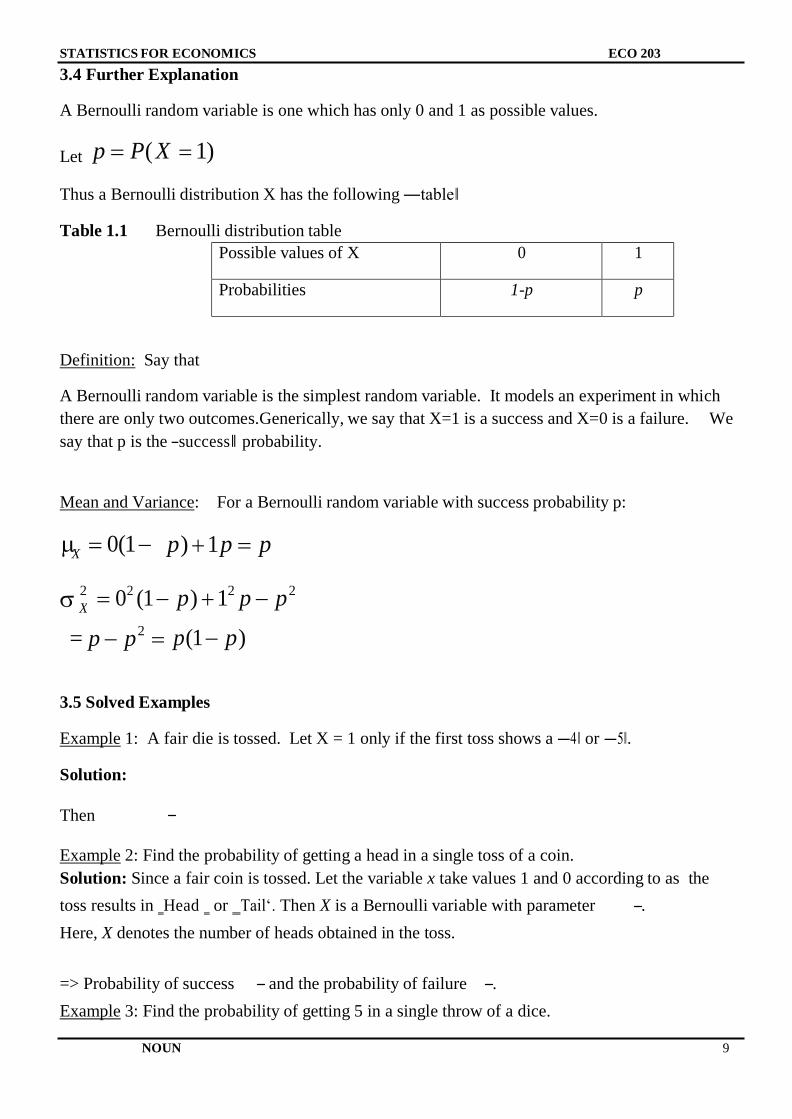
A Bernoulli random variable is one which has only 0 and 1 as possible values.
Let p P( X 1)
Thus a Bernoulli distribution X has the following ―table‖
Table 1.1 Bernoulli distribution table
Possible values of X 0 1
Probabilities 1-p p
Definition: Say that
A Bernoulli random variable is the simplest random variable. It models an experiment in which
there are only two outcomes.Generically, we say that X=1 is a success and X=0 is a failure. We
say that p is the ―success‖ probability.
Mean and Variance: For a Bernoulli random variable with success probability p:
X 0(1 p) 1 p p
2 02 (1 p) 12 p p2
= p p2
p(1 p)
3.5 Solved Examples
Example 1: A fair die is tossed. Let X = 1 only if the first toss shows a ―4‖ or ―5‖.
Solution:
Then
Example 2: Find the probability of getting a head in a single toss of a coin.
Solution: Since a fair coin is tossed. Let the variable x take values 1 and 0 according to as the
toss results in ‗Head ‗ or ‗Tail‘. Then X is a Bernoulli variable with parameter .
Here, X denotes the number of heads obtained in the toss.
=> Probability of success and the probability of failure .
Example 3: Find the probability of getting 5 in a single throw of a dice.
STATISTICS FOR ECONOMICS ECO 203
NOUN 10
Solution:In a single throw of a die, the outcome ―5‖ is called a success and any other outcome is
called a failure, then the successive throws of a dice will contain Bernoulli trials. Therefore, the
probability of success and the probability of failure
4.0 SUMMARY
In this unit, you are expected to have learnt the essentials and applications of Bernoulli
distribution. Also, learners‘ by now would have been able toidentify Bernoulli distribution
function problems and solve the problems accordingly.
[
5.0 CONCLUSION
In conclusion, the Bernoulli, distribution is a discrete distribution whose corresponding random
variables assume only integer values. These are 0 and 1. It does not assume value such as 1.5. The
Bernoulli distribution as an example of a discrete probability distribution is an appropriate tool in
the analysis of proportions and rates.
6.0 TUTOR-MARKED ASSIGNMENT
1. If a student blindly guesses the answer to a multiple choice test questions taken, the test has
10 questions, each of which has 4 possible answers (only one correct). Do the questions
form a sequence of Bernoulli trials? If so, identify the trial outcomes and the parameter p.
2. An American roulette wheel has 38 slots; 18 are red, 18 are black, and 2 are green. A
gambler plays roulette 15 times, betting on red each time. Do the outcomes form a
sequence of Bernoulli trials? If so, identify the trial outcomes and the parameter p.
STATISTICS FOR ECONOMICS ECO 203
NOUN 11
7.0 REFERENCES /FURTHER READING
Spiegel, M. R.and Stephens L.J. (2008).Statistics.(4th ed.).New York: McGraw Hill press.
Swift L., (1997).Mathematics and Statistics for Business, Management and Finance.(2nd ed.).
London: Macmillan Publishers
McCullagh P. and Nelder J., (1989). Generalized Linear Models, (2nd
ed.). Boca Raton: Chapman
and Hall/CRC. ISBN 0-412-31760-5 Web site:http://en.wikipedia.org/wiki/Bernoulli_distribution
Johnson, N. L., Kotz, S. and Kemp A., (1993).Univariate Discrete Distributions (2nd ed.).
Wiley. ISBN 0-471-54897-9 Web site:http://en.wikipedia.org/wiki/Bernoulli_distribution
STATISTICS FOR ECONOMICS ECO 203
NOUN 12
UNIT 2: BINOMIAL DISTRIBUTION
1.0 Objectives
2.0 Introduction
3.0 Main Content
3.1 Probability Density Function of Binomial Distribution
3.2 The Mean of a Binomial Distribution
3.3 Variance of Binomial Distribution
4.0 Summary
5.0 Conclusion
6.0 Assignment
7.0 References / Further Reading
1.0 OBJECTIVES
The aim of this unit is to enable student understand the meaning of Binomial distribution and
instances when it is applicable.
2.0INTRODUCTION
The Binomial distribution can be used under the following conditions:
(i) The random experiment is performed repeatedly a finite and fixed number of times. In
other words n, number of trials, is finite and fixed.
(ii) The outcome of the random experiment (trial) results in the dichotomous classification
of events. In other words, the outcome of each trial may be classified into two mutually
disjoint categories, called success (the occurrence of the event) and failure (the non-
occurrence of the event). i.e. no middle event.
(iii) All trials are independent i.e. the result of any trial is not affected in any way, by the
result of any trial, is not affected in any way, by the preceding trials and does not affect
the result of succeeding trials.
STATISTICS FOR ECONOMICS ECO 203
NOUN 13
(iv) The probability of success (happening of an event) in any trial is p and is constant for
each trial. q = 1-p, is then termed as the probability of failure (non-occurrence of the
event) and is constant for each trial.
For example, if we toss a fair coin n times (which is fixed and finite) then the outcome of any trial
is one of the mutually exclusive events, viz., head (success) and tail (failure). Furthermore, all the
trials are independent, since the result of any throw of a coin does not affect and is not affected by
the result of other throws. Moreover, the probability of success (head) in any trial is ½, which is
constant for each trial. Hence, the coin tossing problems will give rise to Binomial distribution.
Similarly, dice throwing problems will also conform to Binomial distribution.
More precisely, we expect a Binomial distribution under the following conditions:
(i) n, the number of trials is finite.
(ii) Each trial results in mutually exclusive and exhaustive outcomes termed as success and
failure.
(iii) Trials are independent.
(iv) p, the probability of success is constant for each trial. Then q = 1-p, is the probability of
failure in any trial.
Note: The trials satisfying the above four conditions are also known as Bernoulli trials.
3.0 MAIN CONTENT
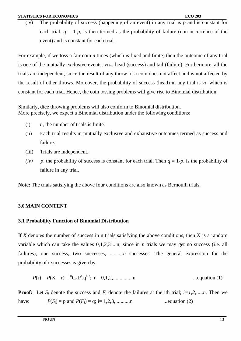
3.1 Probability Function of Binomial Distribution
If X denotes the number of success in n trials satisfying the above conditions, then X is a random
variable which can take the values 0,1,2,3 ...n; since in n trials we may get no success (i.e. all
failures), one success, two successes, ..........n successes. The general expression for the
probability of r successes is given by:
P(r) = P(X = r) = nCr.P
r.q
n-r; r = 0,1,2,...............n ...equation (1)
Proof: Let Si denote the success and Fi denote the failures at the ith trial; i=1,2,.....n. Then we
have: P(Si) = p and P(Fi) = q; i= 1,2,3,...........n ...equation (2)
STATISTICS FOR ECONOMICS ECO 203
NOUN 14
.
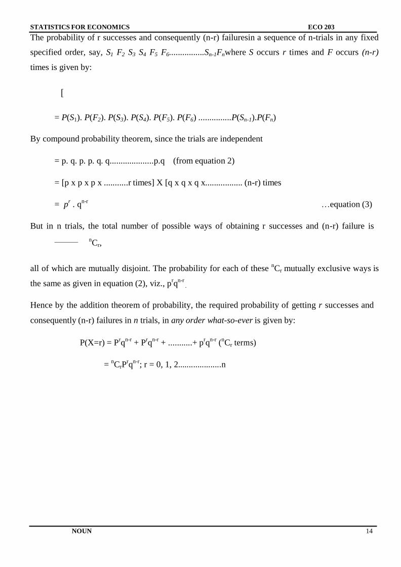
The probability of r successes and consequently (n-r) failuresin a sequence of n-trials in any fixed
specified order, say, S1 F2 S3 S4 F5 F6................Sn-1Fnwhere S occurs r times and F occurs (n-r)
times is given by:
[
= P(S1). P(F2). P(S3). P(S4). P(F5). P(F6) ...............P(Sn-1).P(Fn)
By compound probability theorem, since the trials are independent
= p. q. p. p. q. q....................p.q (from equation 2)
= [p x p x p x ...........r times] X [q x q x q x................. (n-r) times
= pr . q
n-r …equation (3)
But in n trials, the total number of possible ways of obtaining r successes and (n-r) failure is
nCr,
all of which are mutually disjoint. The probability for each of these nCr mutually exclusive ways is
the same as given in equation (2), viz., prq
n-r
Hence by the addition theorem of probability, the required probability of getting r successes and
consequently (n-r) failures in n trials, in any order what-so-ever is given by:
P(X=r) = Prq
n-r + P
rq
n-r + ...........+ p
rq
n-r (
nCr terms)
= nCrP
rq
n-r; r = 0, 1, 2....................n
STATISTICS FOR ECONOMICS ECO 203
NOUN 15
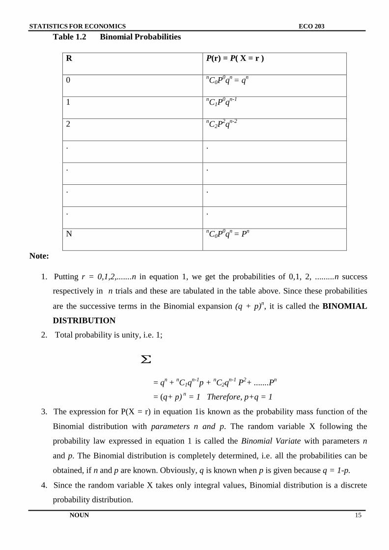
Table 1.2 Binomial Probabilities
R P(r) = P( X = r )
0 nC0P
0q
n = q
n
1 nC1P
0q
n-1
2 nC2P
2q
n-2
. .
. .
. .
. .
N nC0P
0q
n = P
n
Note:
1. Putting r = 0,1,2,.......n in equation 1, we get the probabilities of 0,1, 2, .........n success
respectively in n trials and these are tabulated in the table above. Since these probabilities
are the successive terms in the Binomial expansion (q + p)n, it is called the BINOMIAL
DISTRIBUTION
2. Total probability is unity, i.e. 1;
∑
= qn
+ nC1q
n-1p +
nC2q
n-1 P
2+ .......P
n
= (q+ p) n
= 1 Therefore, p+q = 1
3. The expression for P(X = r) in equation 1is known as the probability mass function of the
Binomial distribution with parameters n and p. The random variable X following the
probability law expressed in equation 1 is called the Binomial Variate with parameters n
and p. The Binomial distribution is completely determined, i.e. all the probabilities can be
obtained, if n and p are known. Obviously, q is known when p is given because q = 1-p.
4. Since the random variable X takes only integral values, Binomial distribution is a discrete
probability distribution.
STATISTICS FOR ECONOMICS ECO 203
NOUN 16
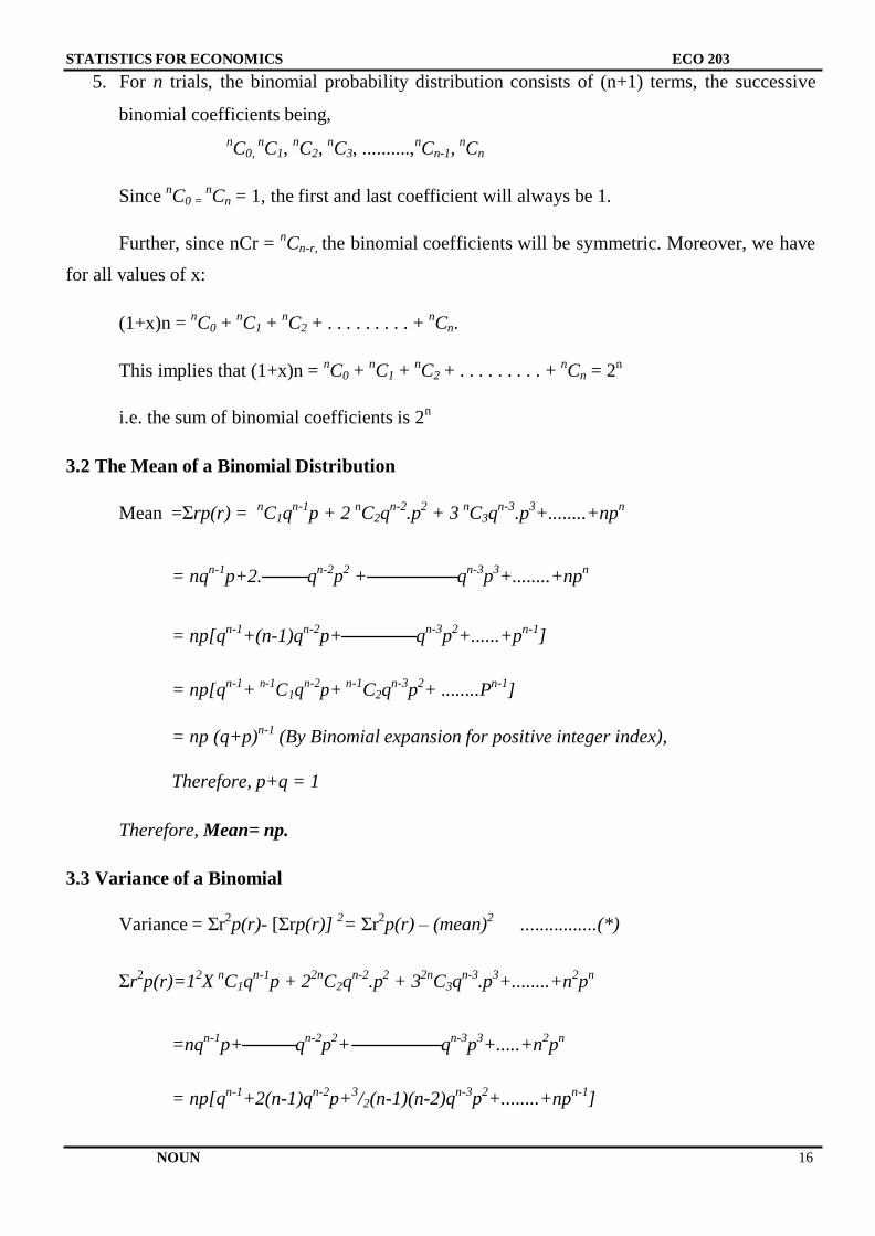
5. For n trials, the binomial probability distribution consists of (n+1) terms, the successive
binomial coefficients being,
nC0,
nC1,
nC2,
nC3, ..........,
nCn-1,
nCn
Since nC0 =
nCn = 1, the first and last coefficient will always be 1.
Further, since nCr = nCn-r, the binomial coefficients will be symmetric. Moreover, we have
for all values of x:
(1+x)n = nC0 +
nC1 +
nC2 + . . . . . . . . . +
nCn.
This implies that (1+x)n = nC0 +
nC1 +
nC2 + . . . . . . . . . +
nCn = 2
n
i.e. the sum of binomial coefficients is 2n
3.2 The Mean of a Binomial Distribution
Mean =Ʃrp(r) = nC1q
n-1p + 2
nC2q
n-2.p
2 + 3
nC3q
n-3.p
3+........+np
n
= nqn-1
p+2. qn-2
p2
+ qn-3
p3+........+np
n
= np[qn-1
+(n-1)qn-2
p+ qn-3
p2+......+p
n-1]
= np[qn-1
+ n-1
C1qn-2
p+ n-1
C2qn-3
p2+ ........P
n-1]
= np (q+p)n-1
(By Binomial expansion for positive integer index),
Therefore, p+q = 1
Therefore, Mean= np.
3.3 Variance of a Binomial
Variance = Ʃr2p(r)- [Ʃrp(r)]
2= Ʃr
2p(r) – (mean)
2 ................(*)
Ʃr2p(r)=1
2X
nC1q
n-1p + 2
2nC2q
n-2.p
2 + 3
2nC3q
n-3.p
3+........+n
2p
n
=nqn-1
p+ qn-2
p2+ q
n-3p
3+.....+n
2p
n
= np[qn-1
+2(n-1)qn-2
p+3/2(n-1)(n-2)q
n-3p
2+........+np
n-1]
STATISTICS FOR ECONOMICS ECO 203
NOUN 17
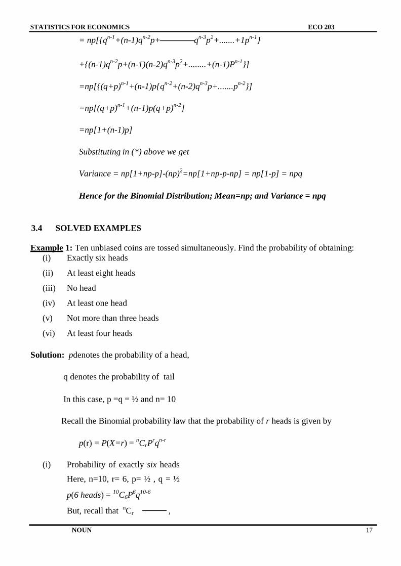
= np[{qn-1
+(n-1)qn-2
p+ qn-3
p2+.......+1p
n-1}
+{(n-1)qn-2
p+(n-1)(n-2)qn-3
p2+........+(n-1)P
n-1}]
=np[{(q+p)n-1
+(n-1)p{qn-2
+(n-2)qn-3
p+.......pn-2
}]
=np[(q+p)n-1
+(n-1)p(q+p)n-2
]
=np[1+(n-1)p]
Substituting in (*) above we get
Variance = np[1+np-p]-(np)2=np[1+np-p-np] = np[1-p] = npq
Hence for the Binomial Distribution; Mean=np; and Variance = npq
3.4 SOLVED EXAMPLES
Example 1: Ten unbiased coins are tossed simultaneously. Find the probability of obtaining:
(i) Exactly six heads
(ii) At least eight heads
(iii) No head
(iv) At least one head
(v) Not more than three heads
(vi) At least four heads
Solution: pdenotes the probability of a head,
q denotes the probability of tail
In this case, p =q = ½ and n= 10
Recall the Binomial probability law that the probability of r heads is given by
p(r) = P(X=r) = nCrP
rq
n-r
(i) Probability of exactly six heads
Here, n=10, r= 6, p= ½ , q = ½
p(6 heads) = 10
C6P6q
10-6
But, recall that nCr ,
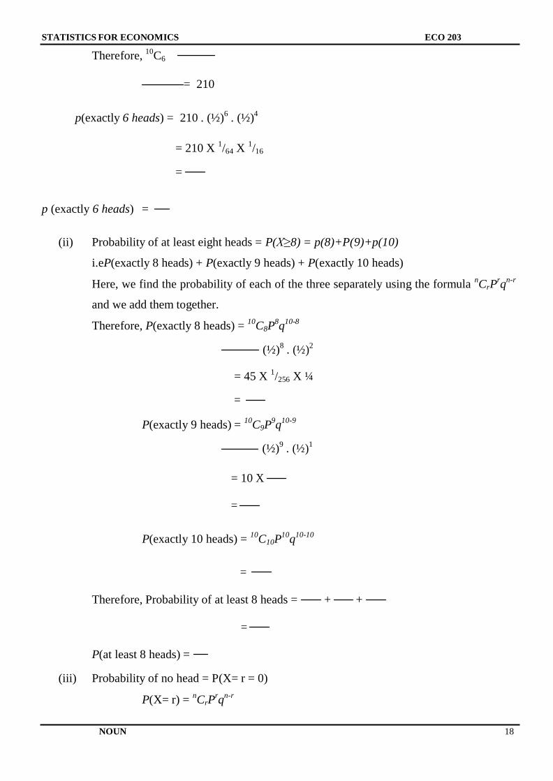
STATISTICS FOR ECONOMICS ECO 203
NOUN 18
Therefore, 10
C6
= 210
p(exactly 6 heads) = 210 . (½)6
. (½)4
= 210 X 1/64 X
1/16
=
p (exactly 6 heads) =
(ii) Probability of at least eight heads = P(X≥8) = p(8)+P(9)+p(10)
i.eP(exactly 8 heads) + P(exactly 9 heads) + P(exactly 10 heads)
Here, we find the probability of each of the three separately using the formula nCrP
rq
n-r
and we add them together.
Therefore, P(exactly 8 heads) = 10
C8P8q
10-8
(½)8
. (½)2
= 45 X 1/256 X ¼
=
P(exactly 9 heads) = 10
C9P9q
10-9
(½)9
. (½)1
= 10 X
=
P(exactly 10 heads) = 10
C10P10
q10-10
=
Therefore, Probability of at least 8 heads = + +
=
P(at least 8 heads) =
(iii) Probability of no head = P(X= r = 0)
P(X= r) = nCrP
rq
n-r
STATISTICS FOR ECONOMICS ECO 203
NOUN 19
P( 0 head) = 10
C0P0q
10-0
= 1 X 1 X
P(0 head) =
(iv) Probability of at least one head
= 1 – P[No head]
= 1 – P(0)
Recall that P(0) =
= 1 -
= 1 -
=
(v) Probability of not more than three heads
= P(X≤3) = P(0) + P(1) + P(2) + P(3)
= [10
C0 + 10
C1 + 10
C2 + 10
C3] =
= =
(vi) Probability (at least 4 heads) = (X ≥4) = 1 – P (X≤3)
= 1 – [p(0) + p(1) + p(2) + p(3)] = 1 -
=
4.0 SUMMARY
In this unit, learners have been made to understand that a Binomial Distribution is the sum of
Independent Bernoulli Random Variables and that the Binomial distribution describes
thedistribution of binary data from a finite sample. Thus it gives the probability of getting r events
out of n trials. In summary, the binomial distribution describes the behaviour of a count variable X
if the following conditions apply:
1. The number of observations n is fixed.
STATISTICS FOR ECONOMICS ECO 203
NOUN 20
2. Each observation is independent.
3. Each observation represents one of two outcomes ("success" or "failure").
4. The probability of "success" p is the same for each outcome.
If in your application of Binomial these conditions are met, then X has a Binomial distribution
with parameters n and p, abbreviated B(n, p).
5.0 CONCLUSION
In probability theory and statistics, the Binomial distribution is the discrete probability
distribution of the number of successes in a sequence of nindependent yes/no experiments, each of
which yields success with probabilityp. Such a success/failure experiment is also called a
Bernoulli experiment or Bernoulli trial; when n = 1, the binomial distribution is a Bernoulli
distribution. The binomial distribution is the basis for the popular binomial test of statistical
significance. The Binomial distribution is frequently used to model the number of successes in a
sample of size n drawn with replacement from a population of size N. If the sampling is carried
out without replacement, the draws are not independent and so the resulting distribution is a
hypergeometric distribution, not a binomial one. However, for N much larger than n, the binomial
distribution is a good approximation, and widely used.
6.0 TUTOR-MARKED ASSIGNMENT
1. Define Binomial Distribution. What is the probability of guessing correctly at least six of the
ten answers in a TRUE-FALSE objective test?
2. A merchant‘s file of 20 accounts contains 6 delinquent and 14 non-delinquent accounts. An
auditor randomly selects 5 of these accounts for examination.
(i) What is the probability that the auditor finds exactly 2 delinquent accounts?
(ii) Find the expected number of delinquent accounts in the sample selected?
(iii) What is the variance of the distribution?
STATISTICS FOR ECONOMICS ECO 203
NOUN 21
7.0 REFERENCES/FURTHER READINGS
Spiegel, M. R. and Stephens L.J. (2008).Statistics.(4th ed.).New York, McGraw Hill.
Gupta S.C. (2011). FundamentalsofStatistics.(6th
Rev. and Enlarged ed.). Mumbai India:
Himalayan Publishing House
Swift L. (1997).Mathematics and Statistics for Business, Management and
Finance.London,Macmillan
STATISTICS FOR ECONOMICS ECO 203
NOUN 22
UNIT 3: NORMAL DISTRIBUTION
1.0 Objectives
2.0 Introduction
3.0 Main Content
3.1 Properties of Normal Distribution
3.2 Relationship between Binomial and normal distribution
4.0 Summary
5.0 Conclusion
6.0 Assignment
7.0 References/Further Reading
1.0 OBJECTIVE
The main aim of this unit is to ensure students‘ proper understanding of normal distribution;
appreciate its applicability in day-to-day business and scientific live and be able to use it as
appropriate in practical statistical studies
2.0 INTRODUCTION
The Normal probability distribution commonly called the normal distribution is one of the most
important continuous the theoretical distributions in Statistics. Most of the data relating to
economic and business statistics or even in the social and physical sciences conform to this
distribution. The normal distribution was first discovered by English Mathematician De-voire
(1667-1754) in 1733 who obtained the mathematical equation for this distribution while dealing
with problems arising in the game of chance. Normal distribution is also known as Gaussian
distribution (Gaussian Law of Errors) after Karl Friedrich Gauss (1777-1855) who used the
distribution to describe the theory of accidental errors of measurements involved in the calculation
of orbits of heavenly bodies.
Today, normal probability model is one of the most important probability models in statistical
analysis. Its graph, called the normal curve is shown below:
STATISTICS FOR ECONOMICS ECO 203
NOUN 23
Y 0.4
0.3
0.2
0.1
-3 -2 -1 1 2 3 Z
68.27%
95.45%
99.73%
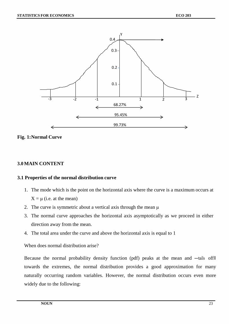
Fig. 1:Normal Curve
3.0 MAIN CONTENT
3.1 Properties of the normal distribution curve
1. The mode which is the point on the horizontal axis where the curve is a maximum occurs at
X = μ (i.e. at the mean)
2. The curve is symmetric about a vertical axis through the mean μ
3. The normal curve approaches the horizontal axis asymptotically as we proceed in either
direction away from the mean.
4. The total area under the curve and above the horizontal axis is equal to 1
When does normal distribution arise?
Because the normal probability density function (pdf) peaks at the mean and ―tails off‖
towards the extremes, the normal distribution provides a good approximation for many
naturally occurring random variables. However, the normal distribution occurs even more
widely due to the following:
STATISTICS FOR ECONOMICS ECO 203
NOUN 24
1. The total (and also the average) of a large number of random variables which have the
same probability distribution approximately has a normal distribution. For instance, if the
amount taken by a shop in a day has particular (maybe unknown) distribution, the total of
100 days‘ takings is the sum of 100 identically distributed random variables and so it will
(approximately) have a normal distribution. Many random variables are normal because of
this. For example, the amount of rainfall which falls during a month is the total of the
amounts of rainfall which have fallen each day or each hour of the month and so is likely to
have a normal distribution. In the same way the average or total of a large sample will
usually have a normal distribution. This can be explored further by further readings on
populations and samples
2. The normal distribution provides approximate probabilities for the binomial distribution
when n, the number of trials is large.
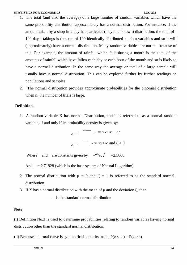
Definitions
1. A random variable X has normal Distribution, and it is referred to as a normal random
variable, if and only if its probability density is given by:
, - ∞ <x< ∞ or √
, - ∞ <x< ∞ and ζ > 0 √
Where and are constants given by =22
/7 ,√ =2.5066
And = 2.71828 (which is the base system of Natural Logarithm)
2. The normal distribution with μ = 0 and ζ = 1 is referred to as the standard normal
distribution.
3. If X has a normal distribution with the mean of μ and the deviation ζ, then
is the standard normal distribution
Note
(i) Definition No.3 is used to determine probabilities relating to random variables having normal
distribution other than the standard normal distribution.
(ii) Because a normal curve is symmetrical about its mean, P(z < -a) = P(z > a)
STATISTICS FOR ECONOMICS ECO 203
NOUN 25
(iii) P(z < a) + P(z > a) = 1.0000
(iv) Only values of P(z < a) are shown in most statistical tables. For P(z > a), 1- P(z < a) is used.
Students are implored to make copies of normal tables from any standard statistic textbook.
Example
1. Using normal tables, find the values of the following probabilities:
(a) P(z < 0.50)
(b) P(z < -2.50)
(c) P(1.62 < z < 2.20)
(d) P(-1.50 < z < 2.50)
(e) P(z > 0.50)
Solution
(a) P(z < 0.50) = 0.6915
i.e read directly from statistical table
(b) P(z < -2.50) = 0.0062
(c) P(1.62 < z < 2.20)
= P(z < 2.20) – P(z < 1.62)
0.9861 – 0.9474
0.0387
(d) P(-1.50 < z < 2.50)
= P(z < 2.50) – P(z < -1.50)
= 0.9938 – 0.0668
= 0.9270
(e) P( z > 0.50)
Because most tables only provide for P(z < 0.50), we shall therefore apply:
P(z > 0.50) = 1- P(z < 0.50)
= 1 – 0.6915
= 0.3085
2. Given a normal distribution with mean of 230 and standard deviation of 20, what is the
probability that an observation from this population is:
(a) Greater than 280
STATISTICS FOR ECONOMICS ECO 203
NOUN 26
(b) Less than = 220
(c) Lies between 220 and 280
Solution
(a)
X = 280, μ= 230, ζ = 20
Therefore, Z =
=2.50
Therefore, P(X > 280) = P(z > 2.50)
= 1 – P(z < 2.50)
= 1 – 0.9938
= 0.0062
(b) P(X < 220)
Z =
= -0.50
Therefore, P(X < 220) = P(z < -0.50)
= 0.3085
(c) P(220 < X < 280)
= P(-0.50 < z < 2.50)
= P(z < 2.50) - P(z < -0.50)
= 0.9938 – 0.3085
= 0.6853
3.2 Relation between Binomial and Normal Distribution
Normal Distribution is a limiting case of the binomial probability distribution under the following
conditions:
(i) n, the number of trials is indefinitely large, i.e.n ∞.
(ii) Neither p nor q is very small.
STATISTICS FOR ECONOMICS ECO 203
NOUN 27
We know that for a binomial variate X with parameter n and p.
E(X) = np and Var(X) = npq
De-Moivre proved that under the above two conditions, the distribution of standard Binomial
variate
√
tends to the distribution of standard Normal variate.
If p and q are nearly equal (i.e., p is nearly ½), the normal approximation is surprisingly good
even for small values of n. However, then p and q are not equal, i.e. when p or q is small, even
then the Binomial distribution tends to normal distribution but in this case the convergence is
slow. By this we mean that if p and q are not equal then for Binomial distribution to tend to
Normal distribution we need relatively larger value of n as compared to the value of n required in
the case when p and q are nearly equal. Thus, the normal approximation to the Binomial
distribution is better for increasing values of n and is exact in the limiting case as n ∞.
In the light of the above, binomial related problems can be solve through Poisson approximation
using a combination of both.
4.0 SUMMARY
In summary, learners would have understood that the normal distribution can be described
completely by the two parameters .The mean is the center of the distribution and the
standard deviation is the measure of the variation around the mean.
5.0 CONCLUSION
The normal distribution is the most important distribution. It describes well thedistribution of
random variables that arise in practice, such as the heights or weightsof people, the total annual
sales of a firm, exam scores etc. Also, it is important for thecentral limit theorem, the
approximation of other distributions such as the binomial, etc.
STATISTICS FOR ECONOMICS ECO 203
NOUN 28
6.0 TUTOR-MARKED ASSIGNMENT
1. Suppose the monthly salaries of 500 parents of students in a Senior School are normally
distributed with mean N63,000 and standard deviation of N7,500. Find:
(a) The probability of a parent‘s salary lying between N59,500 and N66,000
(b) Probability of a parent‘s salary greater than or equal to N65,000
(c) Find the number of parents with monthly salaries between N62,000 and N67,000
2. Time taken by the crew of a company to construct a small bridge is a normal variate with a
mean of 400 labour hours and a standard deviation of 100 labour hours.
(i) What is the probability that the bridge is constructed between 350 and 450 labour
hours?
(ii) If the company promises to construct a bridge in 450 labour hours or less and agrees
to pay a penalty of N1,000 for each labour hour spent in excess of 450, what is the
probability that the company pays a penalty of at least N20,000
3. The National Bureau for Economic Data is organizing a stakeholder symposium on how to
tackle the problem of dearth of reliable economic data in Nigeria. The Director of Accounts
states that they can afford to entertain no more than 200 guests at the symposium, and the hotel
at which it is to be held will only cater for a minimum of 140 guests. The public Relation unit
of the Bureau is to send invitation to 240 people. The Statistics, Planning and Research unit of
the Bureau estimates that the probability each individual accepts the invitation is about 70%.
Using this model, estimate the probability that between 140 and 200 guests accept the
invitation. Is 240 a good number of invitations to send?
7.0 REFERENCES/FURTHER READINGS
Spiegel, M. R. and Stephens L.J. (2008).Statistics.(4th ed.). New York:McGraw Hill Press.
Gupta S.C (2011). Fundamentals of Statistics.(6th
Rev. and Enlarged ed.). Mumbai, India:
Himalayan Publishing House
Swift L. (1997).Mathematics and Statistics for Business, Management and
Finance.London:Macmillan.
STATISTICS FOR ECONOMICS ECO 203
NOUN 29
UNIT 4: POISSON DISTRIBUTION
CONTENTS
1.0 Objectives
2.0 Introduction
3.0 Main Content
3.1 Condition for using Poisson Distribution
3.2 Application
4.0 Summary
5.0 Conclusion
6.0 Assignment
7.0 References/Further Reading
1.0 OBJECTIVES
The main objective of this unit is to enable the students understand the concept of Poisson
distribution, its importance and applications. Students are expected to understand the link between
Poisson distribution and Binomial distribution and the distinguishing features.
2.0 INTRODUCTION
Poisson distribution was derived in 1837 by a French mathematician Simeon D. Poisson (1781 –
1840). Poisson distribution may be obtained as a limiting case of Binomial probability distribution
under the following conditions:
(i) n, the number of trials is indefinitely large i.e.n tends towards infinity
(ii) p, the constant probability of success for each trial is indefinitely small i.e.p tends
towards zero.
(iii) np = μ, is finite
Under the above three conditions the Binomial probability function tends to the probability
function of the Poisson distribution given as:
STATISTICS FOR ECONOMICS ECO 203
NOUN 30
Where X or r is the number of success (occurrences of the event) μ = np and e =2.71828 (the base
of the system of natural logarithm)
3.0 MAIN CONTENT
3.1 Condition for Using Poisson Distribution
The condition under which Poisson distribution is obtained is in a limiting case of Binomial
Distribution. It is applicable in fields such as Queuing Theory (waiting line problems), insurance,
biology, business, Economics and Industry. Some of the practical situation in which the
distribution can be applied include but not limited to:
(i) The number of vehicles arriving at a filling station
(ii) Number of patients arriving at a hospital
(iii) The number of accidents taking place per day on a busy road
(iv) The number of misprint per page of a typed material etc.
3.2 Application
Example 1: The mean number of misprints per page in a book is 1.2. What is the probability of
finding on a particular page?
(a) No misprints
(b) Three or more misprints
Solution
μ = 1.2
(a) Pr (No misprints)
=Pr(X=0)
STATISTICS FOR ECONOMICS ECO 203
NOUN 31
= e-1.2
= 0.301
(b) Pr(or more misprint)
= Pr(X ≥ 3)
= 1 – [Pr(0) + Pr(1) + Pr(2)]
Pr(0) = 0.301 as in (a) above
Pr(1)
= 0.3612
Pr(2)=
= 0.21672
Pr (0) + Pr(1) + Pr(2) = 0.87892
Therefore, Pr(X ≥ 3) = 1 - 0.87892
= 0.12108
= 0.121
4.0 SUMMARY
In this unit, student must have learnt the rudiments and applications of Poisson distribution.
Students are must have learnt how to solve problems using Poisson distribution.
5.0 CONCLUSION
In conclusion Poisson distribution is a limiting case of Binomial distribution, it can be applied in
cases when the number is very large tending towards infinity and the probability of success is very
low.
STATISTICS FOR ECONOMICS ECO 203
NOUN 32
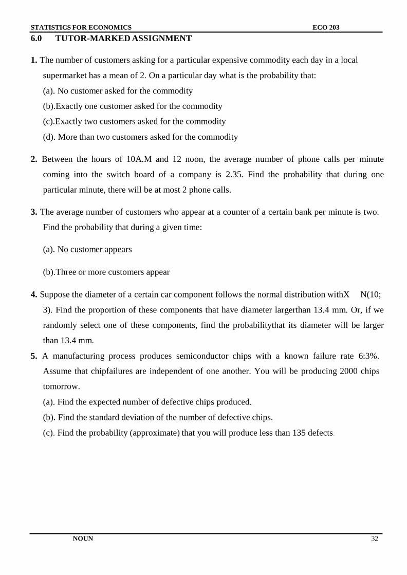
6.0 TUTOR-MARKED ASSIGNMENT
1. The number of customers asking for a particular expensive commodity each day in a local
supermarket has a mean of 2. On a particular day what is the probability that:
(a). No customer asked for the commodity
(b).Exactly one customer asked for the commodity
(c).Exactly two customers asked for the commodity
(d). More than two customers asked for the commodity
2. Between the hours of 10A.M and 12 noon, the average number of phone calls per minute
coming into the switch board of a company is 2.35. Find the probability that during one
particular minute, there will be at most 2 phone calls.
3. The average number of customers who appear at a counter of a certain bank per minute is two.
Find the probability that during a given time:
(a). No customer appears
(b).Three or more customers appear
4. Suppose the diameter of a certain car component follows the normal distribution withX N(10;
3). Find the proportion of these components that have diameter largerthan 13.4 mm. Or, if we
randomly select one of these components, find the probabilitythat its diameter will be larger
than 13.4 mm.
5. A manufacturing process produces semiconductor chips with a known failure rate 6:3%.
Assume that chipfailures are independent of one another. You will be producing 2000 chips
tomorrow.
(a). Find the expected number of defective chips produced.
(b). Find the standard deviation of the number of defective chips.
(c). Find the probability (approximate) that you will produce less than 135 defects.
STATISTICS FOR ECONOMICS ECO 203
NOUN 33
7.0 REFERENCES/FURTHER READING
Spiegel, M. R. and Stephens L.J. (2008).Statistics.(4th ed.). New York:McGraw Hill Press.
Gupta S.C. (2011). Fundamentals of Statistics.(6th
Rev. and Enlarged ed.). Mumbai, India:
Himalayan Publishing House.
Swift L. (1997).Mathematics and Statistics for Business, Management and
Finance.London:Macmillan.
STATISTICS FOR ECONOMICS ECO 203
NOUN 34
MODULE 2: STATISTICAL HYPOTHESIS TEST
A statistical hypothesis test is a method of making decisions using data from a scientific study.
In statistics, a result is interpreted as beingstatistically significant if it has been predicted as
unlikely to have occurred by chance alone, according to a pre-determined threshold probability,
the significance level. The phrase "test of significance" was coined by statistician Ronald Fisher.
These tests are used in determining what outcomes of a study would lead to a rejection of the null
hypothesis for a pre-specified level of significance; this can help to decide whether results contain
enough information to cast doubt on conventional wisdom, given that conventional wisdom has
been used to establish the null hypothesis. The critical region of a hypothesis test is the set of all
outcomes which cause the null hypothesis to be rejected in favour of the alternative hypothesis.
Statistical hypothesis testing is sometimes called confirmatory data analysis, in contrast to
exploratory data analysis, which may not have pre-specified hypotheses. Statistical hypothesis
testing is a key technique of frequentist inference.
Statistics are helpful in analyzing most collections of data. This is equally true of hypothesis
testing which can justify conclusions even when no scientific theory exists.
Common test Statistics are; t-test, z-test, chi-square test and f-test which is sometimes referred to
as analysis of variance (ANOVA) test.
In this module, five statistical tests will be discussed and analyzed in order to make learners
appreciate and understand of the different statistical hypothesis tests. These statistical tests are:
Unit 1: T- test
Unit 2: F- test
Unit 3: Chi square test
Unit 4: ANOVA
Unit 5: Parametric and Non-Parametric test Methods
STATISTICS FOR ECONOMICS ECO 203
NOUN 35
UNIT 1: T–TEST
CONTENTS
1.0 Objectives
2.0 Introduction
3.0 Main Content
3.1 Application of t-distribution
3.2 Test for single mean
3.3 Assumptions for Student‘s test
3.4 t-Test for difference of means
4.0 Summary
5.0 Conclusion
6.0 Assignment
7.0 References/Further Reading
1.0 OBJECTIVES
The objective of this unit is to introduce students to t-distribution and emphasize its application in
statistics.
2.0 INTRODUCTION
The Student‘s t-test
For large sample test for mean √
If the population variance is unknown then for the large samples, its estimates provided by sample
variance S2
is used and normal test is applied. For small samples an unbiased estimate of
population variance ζ2
is given by:
∑
It is quite conventional to replace ζ2
byS2
(for small samples) and then apply the normal test even
for small samples. W.S.Goset, who wrote under the pen name of Student, obtained the sampling
STATISTICS FOR ECONOMICS ECO 203
NOUN 36
distribution of the statistic
√
for small samples and showed that it is far from normality. This
discovery started a new field, viz ‗Exact Sample Test‘ in the history of statistical inference.
Note: If x1, x2...............xn is a random sample of size n from a normal population with mean μ and
variance ζ2
then the Student‘s t statistic is defined as:
√ √
Where = is the sample mean and ∑ is an unbiased estimate of the
population variance ζ2
3.0 MAIN CONTENT
3.1 Applications of t-distribution
(i) t-test for the significance of single mean, population variance being unknown
(ii) t-test for the significance of the difference between two sample means, the population
variances being equal but unknown
(iii) t-test for the significance of an observed sample correlation coefficient
3.2 Test for Single Mean
Sometimes, we may be interested in testing if:
(i) the given normal population has a specified value of the population mean, say μo.
(ii) the sample mean differ significantly from specified value of population mean.
(iii) A given random sample x1, x2...............xnof size n has been drawn from a normal
population with specified meanμo.
Basically, all the three problems are the same. We set up the corresponding null hypothesis
thus:
(a) Ho: μ = μoi.e the population mean is μo
STATISTICS FOR ECONOMICS ECO 203
NOUN 37
(b) Ho: There is no significant difference between the sample mean and the population mean.
In order words, the difference between and μ is due to fluctuations of sampling.
(c) Ho: The given random sample has been drawn from the normal population with mean μo.
Under Ho the test-statistic is:
√ √
Where = and ∑
And it follows Student‘s t-distribution with (n-1) degrees of freedom.
We compute the test-statistic using the formula above under Ho and compare it with the tabulated
value of t for (n-1) d.f at the given level of significance. If the absolute value of the calculated t is
greater than tabulated t, we say it is significant and the null hypothesis is rejected. But if the
calculated t is less than tabulated t, Ho may be accepted at the level of significance adopted.
3.3 Assumptions for Student’s test
(i) The parent population from which the sample is drawn is normal
(ii) The sample observations are independent i.e the given sample is random.
(iii) The population standard deviation ζ is unknown
Example: Ten cartons are taken at random from an automatic filling machine. The mean net
weight of the 10 cartons is 11.8kg and standard deviation is 0.15kg. Does the sample mean differ
significantly from the intended weight of 12kg, α=0.05
Hint: You are given that for d.f =9, t0.05 = 2.26
Solution: n= 10, = 11.8kg, s = 0.15kg
Null hypothesis, Ho : μ = 12 kg (i.e the sample mean of =11.8 kg does not differ significantly
from the population mean μ = 12 kg
Alternative Hypothesis.Ho: ≠ 12kg (Two tailed)
STATISTICS FOR ECONOMICS ECO 203
NOUN 38
2
√ √
√
The tabulated value of t for 9 d.f at 5% level of significance is 2.26. Since the the calculated t is
much greater than the tabulated t, it is highly significant. Hence, null hypothesis is rejected at 5%
level of significance and we conclude that the sample mean differ significantly.
3.4t-Test for difference of means
Assume we are interested in testing if two independent samples have been drawn from two normal
populations having the same means, the population variances being equal.
Let x1, x2...............xn and y1, y2...............yn be two independent random samples from the given
normal populations.
Ho: μx = μyi.e the two samples have been drawn from the normal populations with the same
means. Under the hypothesis that the ζ12
= ζ 2
unknown, the test statistic under Ho is:
√
= ζ2i.e population variances are equal but
Where ∑ ∑
And [∑ ∑ ]
is an unbiased estimate of the common population variance ζ2
based on both the samples. By
comparing the computed value of t with the tabulated value of t for n1 + n2 -2 d.f. and at desired
level of significance, usually 5% or 1%, we reject the null hypothesis.
Example: The nicotine content in milligram of two samples of tobacco were found to be as
follows:
STATISTICS FOR ECONOMICS ECO 203
NOUN 39
Sample A: 24 27 26 21 25
Sample B: 27 30 28 31 22 36
Can it be said that the two samples come from the same normal population having the same
mean?
Solution Hints: Applying the above formula and calculating the variance as appropriate, the
calculated t-value is -1.92. the tabulated value for 9 d.f at 5% level of significance for two-tailed
test is 2.262. Since calculated t is less than the tabulated t, it is not significant and the null
hypothesis is accepted.
4.0 SUMMARY
In summary, learners would have learnt how to apply t-test in solving statistical problems such as
test to confirm if mean is a certain value, to test significance of the difference between two mean
among others.
5.0 CONCLUSION
T-testhas very wide applications. It can be applied in the tests of single mean, in the comparison
of two different means and in the test of significance of other parameter estimates.
6.0 TUTOR-MARKED ASSIGNMENT
1. The mean weekly sale of the chocolate bar in candy stores was 146.3 bars per store. After
advertising campaign the mean weekly sales in 22 stores for typical week increased to 153.7
and showed a standard deviation of 17.2. Was the advertising campaign successful?
2. Prices of shares of a company on the different days in a month were found to be: 66, 65, 69,
70, 69, 71, 70, 63, 64 and 68. Discuss whether the mean price of the price of the shares in the
month is 65.
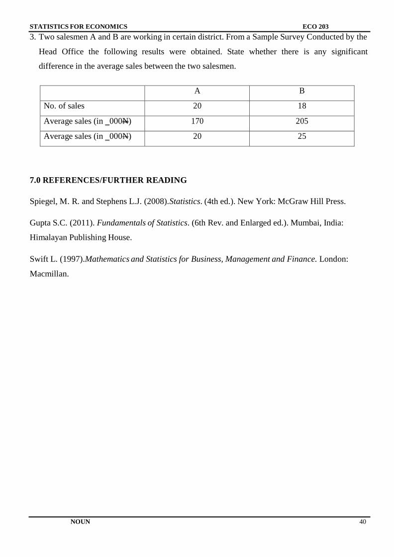
STATISTICS FOR ECONOMICS ECO 203
NOUN 40
3. Two salesmen A and B are working in certain district. From a Sample Survey Conducted by the
Head Office the following results were obtained. State whether there is any significant
difference in the average sales between the two salesmen.
A B
No. of sales 20 18
Average sales (in ‗000N) 170 205
Average sales (in ‗000N) 20 25
7.0 REFERENCES/FURTHER READING
Spiegel, M. R. and Stephens L.J. (2008).Statistics. (4th ed.). New York: McGraw Hill Press.
Gupta S.C. (2011). Fundamentals of Statistics. (6th Rev. and Enlarged ed.). Mumbai, India:
Himalayan Publishing House.
Swift L. (1997).Mathematics and Statistics for Business, Management and Finance. London:
Macmillan.
STATISTICS FOR ECONOMICS ECO 203
NOUN 41
UNIT 2: F-TEST
CONTENTS
1.0 Objectives
2.0 Introduction
3.0 Main Content
3.1 Applications of the F-distribution
3.2 For testing equality of population variances
4.0 Summary
5.0 Conclusion
6.0 Assignment
7.0 References/Further Reading
1.0 OBJECTIVE
The main objective of this section is to introduce student to the world of F-distribution and learn
its theories and application to day-to-day business and economic problems.
2.0 INTRODUCTION
In F-TEST, If X is a χ2-variate with n1 degree of freedom and Y is an independent χ
2-variate with
n2 degree of freedom, then F-statistic is defined as:
i.e. F-statistic is the ratio of two independent chi-square variates divided by their respective
degrees of freedom. The statistic follows G.W Snedecor‘s F-distribution with (n1, n2)degree of
freedom with probability density function given by:
Where is a constant which is so determined that total area under the probability curves is 1 i.e
∫
STATISTICS FOR ECONOMICS ECO 203
NOUN 42
Note: The sampling distribution of F-statistics does not involve any population parameters and
depends only on the degrees of freedom n1 and n2. The graph of the function p(F) varies with the
degree of freedom n1 and n2.
Critical values of F-distribution: The available F-tables in most standard statistical table give
the critical values of F for the right-tailed test, i.e the critical region is determined by the right tail
areas. Thus, the significant value Fα (v1,v2) at level of significance α and (v1,v2) d.f. 2 is
determined by the equation:
[ ]
Significant values of the variance-Ratio
3.0 MAIN CONTENT
3.1 Applications of the F-distribution
F-distribution has a number of applications in the field of statistics. This includes but not limited
to the following:
(1) To test for equality of population variances
(2) To the equality of several populations means i.e. for testing Ho: μ1 = μ2 =...= μk.
This is by far the most important application of F-statistic and is done through the
technique of Analysis of Variance (ANOVA). This shall be treated as a separate unit
later.
(3) For testing the significance of an observed sample multiple correlation
(4) For testing the significance of an observed sample correlation ratio
3.2 For testing equality of population variances: Here, we set up the Null hypothesis Ho: ζ1=
ζ2 = ζi.e population variances are the same. In other words, Ho is that the two independent
estimates of the common population variance do not differ significantly.
Under Ho, the test statistic is
where and are unbiased estimates of the common population variance ζ2
and are given by:
∑ ∑
and it follows Snedecor‘s F-distribution with v1 =n1-1, v2 =n2-1 d.f.; i.e F ~F(v1, v2)
STATISTICS FOR ECONOMICS ECO 203
NOUN 43
1 2
1
Since F-test is based on the ratio of two variances, it is also known as variance ratio test.
Assumption for F-test for equality of variances
1. The samples are simple random samples
2. The samples are independent of each other
3. The parent populations from which the samples are drawn are normal
N.B (1) Since the most available tables of the significant values of F are for the right-tail test, i.e
against the alternative Ho : ζ 2
> ζ 2, in numerical problems we will take greater of the variances
or as the numerator and adjust for the degree of freedom accordingly. Thus, in F ~ (v1, v2),
v1 refers to the degree of freedom of the larger variance, which must be taken as the numerator
while computing F.
If Ho is true i.e ζ 2
= ζ22
= ζ2
the value of F should be around 1, otherwise, it should be greater
than 1. If the value of F is far greater than 1 the Ho should be rejected. Finally, if we take larger of
or as the numerator, all the tests based on the F-statistic become right tailed tests.
- All one tailed tests for Ho at level of significance ―α‖ will be right tailed tests only with
area ―α‖ in the right.
- For two-tailed tests, the critical value is located in the right tail of F-distribution with
area (α/2) in the right tail.
Example 1: The time taken (in minutes) by drivers to drive from Town A to Town B driving two
different types of cars X and Y is given below
Car Type X: 20 16 26 27 23 22
Car Type Y: 27 33 42 35 32 34 38
Do the data show that the variances of time distribution from population from which the samples
are drawn do not differ significantly?
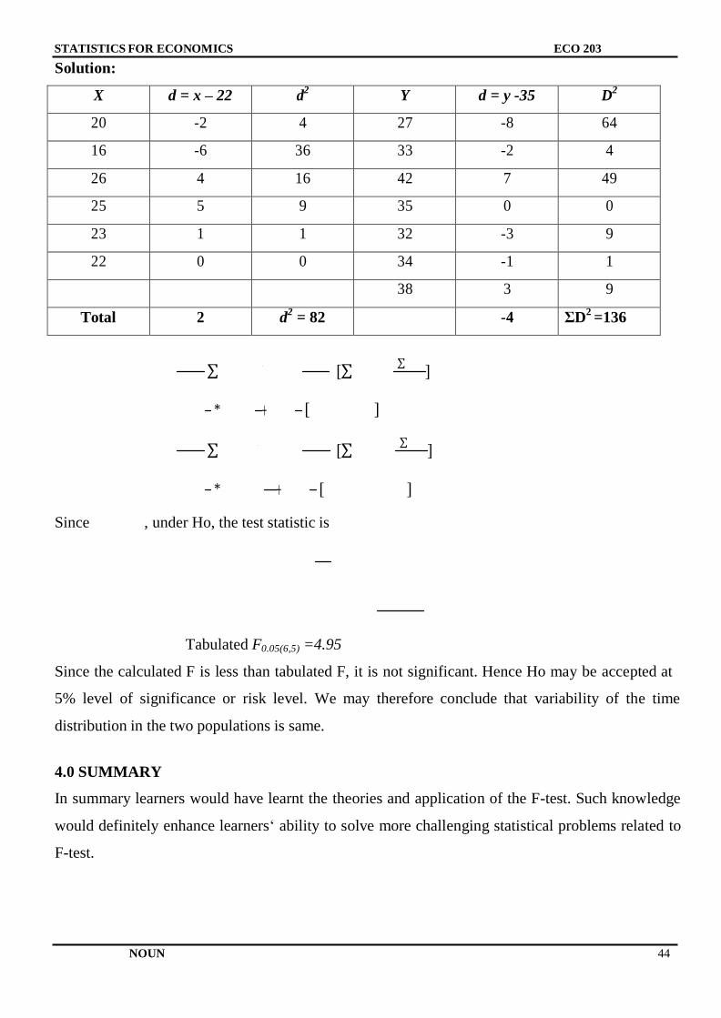
STATISTICS FOR ECONOMICS ECO 203
NOUN 44
Solution:
X d = x – 22 d2 Y d = y -35 D
2
20 -2 4 27 -8 64
16 -6 36 33 -2 4
26 4 16 42 7 49
25 5 9 35 0 0
23 1 1 32 -3 9
22 0 0 34 -1 1
38 3 9
Total 2 d2
= 82 -4 ΣD2
=136
∑ [∑ ∑
]
* + [ ]
∑ [∑
∑ ]
* + [ ]
Since , under Ho, the test statistic is
Tabulated F0.05(6,5) =4.95
Since the calculated F is less than tabulated F, it is not significant. Hence Ho may be accepted at
5% level of significance or risk level. We may therefore conclude that variability of the time
distribution in the two populations is same.
4.0 SUMMARY
In summary learners would have learnt the theories and application of the F-test. Such knowledge
would definitely enhance learners‘ ability to solve more challenging statistical problems related to
F-test.
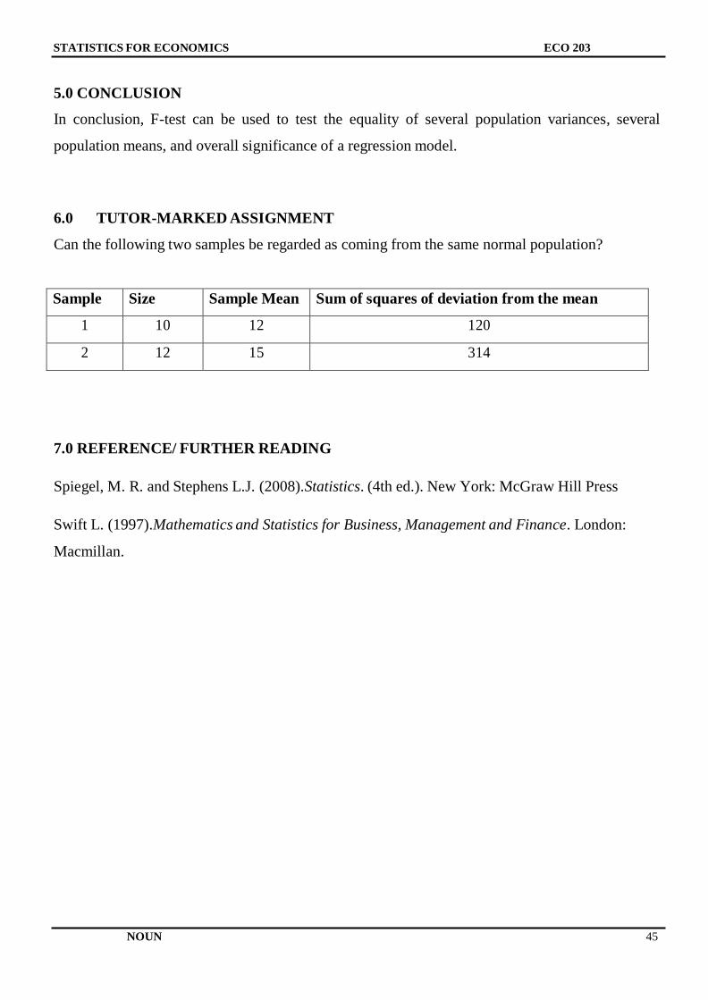
STATISTICS FOR ECONOMICS ECO 203
NOUN 45
5.0 CONCLUSION
In conclusion, F-test can be used to test the equality of several population variances, several
population means, and overall significance of a regression model.
6.0 TUTOR-MARKED ASSIGNMENT
Can the following two samples be regarded as coming from the same normal population?
Sample Size Sample Mean Sum of squares of deviation from the mean
1 10 12 120
2 12 15 314
7.0 REFERENCE/ FURTHER READING
Spiegel, M. R. and Stephens L.J. (2008).Statistics. (4th ed.). New York: McGraw Hill Press
Swift L. (1997).Mathematics and Statistics for Business, Management and Finance. London:
Macmillan.
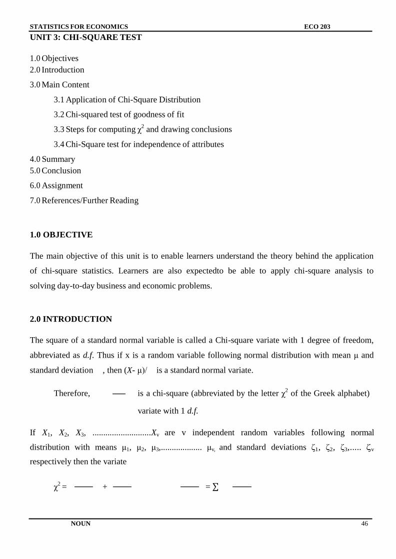
STATISTICS FOR ECONOMICS ECO 203
NOUN 46
UNIT 3: CHI-SQUARE TEST
1.0 Objectives
2.0 Introduction
3.0 Main Content
3.1 Application of Chi-Square Distribution
3.2 Chi-squared test of goodness of fit
3.3 Steps for computing χ2
and drawing conclusions
3.4 Chi-Square test for independence of attributes
4.0 Summary
5.0 Conclusion
6.0 Assignment
7.0 References/Further Reading
1.0 OBJECTIVE
The main objective of this unit is to enable learners understand the theory behind the application
of chi-square statistics. Learners are also expectedto be able to apply chi-square analysis to
solving day-to-day business and economic problems.
2.0 INTRODUCTION
The square of a standard normal variable is called a Chi-square variate with 1 degree of freedom,
abbreviated as d.f. Thus if x is a random variable following normal distribution with mean μ and
standard deviation , then (X- μ)/ is a standard normal variate.
Therefore, is a chi-square (abbreviated by the letter χ2
of the Greek alphabet)
variate with 1 d.f.
If X1, X2, X3, ...........................Xv are v independent random variables following normal
distribution with means μ1, μ2, μ3,................... μv, and standard deviations ζ1, ζ2, ζ3,..... ζv
respectively then the variate
χ2
= + = ∑
STATISTICS FOR ECONOMICS ECO 203
NOUN 47
which is the sum of the squares of v independent standard normal variates, follow Chi-square
distribution with v d.f
3.0 MAIN CONTENTS
3.1 Applications of the χ2-Distribution
Chi-square distribution has a number of applications, some of which are enumerated below:
(i) Chi-square test of goodness of fit.
(ii) χ2-test for independence of attributes
(iii) To test if the population has a specified value of variance ζ2.
(iv) To test the equality of several population proportions
Observed and Theoretical Frequencies
Suppose that in a particular sample a set of possible events E1, E2, E3,..................Ek are observed
to occur with frequencies O1, O2, O3, ..........Ok, called observed frequencies, and that according to
probability rules they are expected to occur with frequencies e1, e2, e3,.....ek, called expected or
theoretical frequencies. Often we wish to know whether the observed frequencies differ
significantly from expected frequencies.
Definition of χ2
A measure of discrepancy existing between the observed and expected frequencies is supplied by
the statistics χ2
given by
χ2
=
3.2 Chi-Square test of goodness of fit
The chi-square test can be used to determine how well theoretical distributions 9such as the
normal and binomial distributions) fit empirical distributions (i.e. those obtained from sample
data). Suppose we are given a set of observed frequencies obtained under some experiment and
we want to test if the experimental results support a particular hypothesis or theory. Karl Pearson
in 1900, developed a test for testing the significance of the discrepancy between experimental
values and the theoretical values obtained under some theory or hypothesis. This test is known as
STATISTICS FOR ECONOMICS ECO 203
NOUN 48
χ2-test of goodness of fit and is used to test if the deviation between observation (experiment) and
theory may be attributed to chance (fluctuations of sampling) or if it is really due to the
inadequacy of the theory to fit the observed data.
Under the null hypothesis that there is no significant difference between the observed
(experimental and the theoretical or hypothetical values i.e there is good compatibility between
theory and experiment.
Karl Pearson proved that the statistic
χ2 = ∑
=
Follows χ2-distribution with v = n-1, d.f where O1, O2,..................On are the observed frequencies
and E1, E2,..................En are the corresponding expected or theoretical frequencies obtained under
some theory or hypothesis.
3.3 Steps for computing χ2
and drawing conclusions
(i) Compute the expected frequencies E1, E2, .....................En corresponding to the
observed frequencies O1, O2, ...................On under some theory or hypothesis
(ii) Compute the deviations (O-E) for each frequency and then square them to obtain (O-
E)2.
(iii) Divide the square of the deviations (O-E)2
by the corresponding expected frequency to
obtain (O-E)2/E.
(iv) Add values obtained in step (iii) to compute χ2 = ∑
(v) Under the null hypothesis that the theory fits the data well, the statistic follows χ
2-
distribution with v = n-1 d.f
(vi) Look for the tabulated (critical) values of χ2
for (n-1) d.f at certain level of significance,
usually 5% or 1%, from any Chi-square distribution table.
If calculated value of χ2
obtained in step (iv) is less than the corresponding tabulated
value obtained in step (vi), then it is said to be non-significant at the required level of
significance. This implies that the discrepancy between observed values (experiment)
and the expected values (theory) may be attributed to chance, i.e fluctuations of
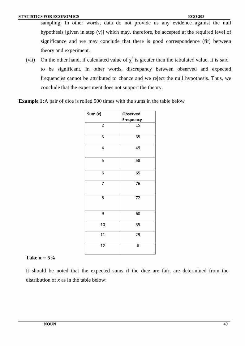
STATISTICS FOR ECONOMICS ECO 203
NOUN 49
sampling. In other words, data do not provide us any evidence against the null
hypothesis [given in step (v)] which may, therefore, be accepted at the required level of
significance and we may conclude that there is good correspondence (fit) between
theory and experiment.
(vii) On the other hand, if calculated value of χ2
is greater than the tabulated value, it is said
to be significant. In other words, discrepancy between observed and expected
frequencies cannot be attributed to chance and we reject the null hypothesis. Thus, we
conclude that the experiment does not support the theory.
Example 1:A pair of dice is rolled 500 times with the sums in the table below
Sum (x) Observed Frequency
2 15
3 35
4 49
5 58
6 65
7 76
8 72
9 60
10 35
11 29
12 6
Take α = 5%
It should be noted that the expected sums if the dice are fair, are determined from the
distribution of x as in the table below:
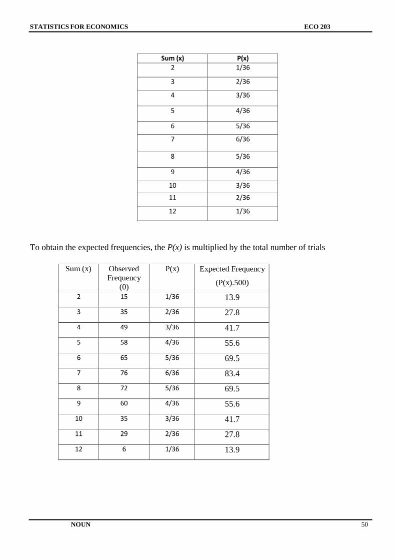
STATISTICS FOR ECONOMICS ECO 203
NOUN 50
Sum (x) P(x) 2 1/36
3 2/36
4 3/36
5 4/36
6 5/36
7 6/36
8 5/36
9 4/36
10 3/36
11 2/36
12 1/36
To obtain the expected frequencies, the P(x) is multiplied by the total number of trials
Sum (x) Observed
Frequency
(0)
P(x) Expected Frequency
(P(x).500)
2 15 1/36 13.9
3 35 2/36 27.8
4 49 3/36 41.7
5 58 4/36 55.6
6 65 5/36 69.5
7 76 6/36 83.4
8 72 5/36 69.5
9 60 4/36 55.6
10 35 3/36 41.7
11 29 2/36 27.8
12 6 1/36 13.9
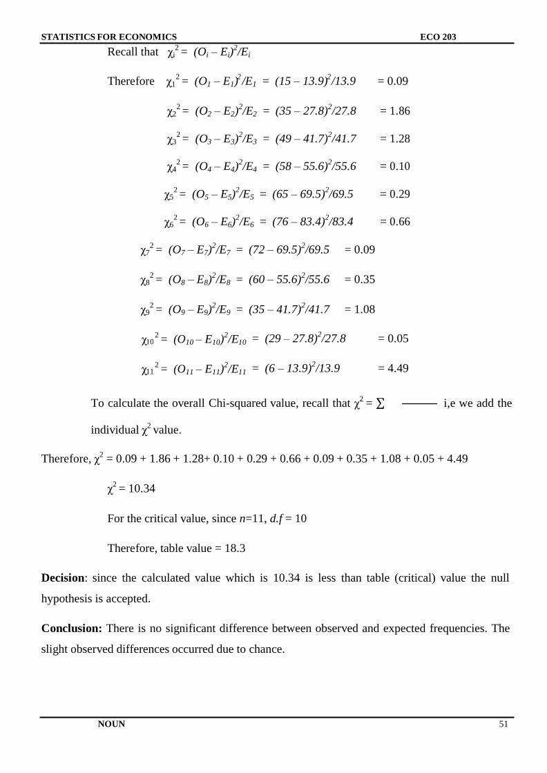
STATISTICS FOR ECONOMICS ECO 203
NOUN 51
10
11
Recall that χi2 = (Oi – Ei)
2/Ei
2 2 2
Therefore χ1 = (O1 – E1) /E1 = (15 – 13.9) /13.9 = 0.09
χ22 = (O2 – E2)
2/E2 = (35 – 27.8)
2/27.8 = 1.86
χ32 = (O3 – E3)
2/E3 = (49 – 41.7)
2/41.7 = 1.28
χ42 = (O4 – E4)
2/E4 = (58 – 55.6)
2/55.6 = 0.10
χ52 = (O5 – E5)
2/E5 = (65 – 69.5)
2/69.5 = 0.29
χ62 = (O6 – E6)
2/E6 = (76 – 83.4)
2/83.4 = 0.66
χ72 = (O7 – E7)
2/E7 = (72 – 69.5)
2/69.5 = 0.09
χ82 = (O8 – E8)
2/E8 = (60 – 55.6)
2/55.6 = 0.35
χ92 = (O9 – E9)
2/E9 = (35 – 41.7)
2/41.7 = 1.08
χ 2 = (O10 – E10)
2/E10 = (29 – 27.8)
2/27.8 = 0.05
χ 2 = (O11 – E11)
2/E11 = (6 – 13.9)
2/13.9 = 4.49
To calculate the overall Chi-squared value, recall that χ2
= ∑ i,e we add the
individual χ
2 value.
Therefore, χ2
= 0.09 + 1.86 + 1.28+ 0.10 + 0.29 + 0.66 + 0.09 + 0.35 + 1.08 + 0.05 + 4.49
χ2 = 10.34
For the critical value, since n=11, d.f = 10
Therefore, table value = 18.3
Decision: since the calculated value which is 10.34 is less than table (critical) value the null
hypothesis is accepted.
Conclusion: There is no significant difference between observed and expected frequencies. The
slight observed differences occurred due to chance.
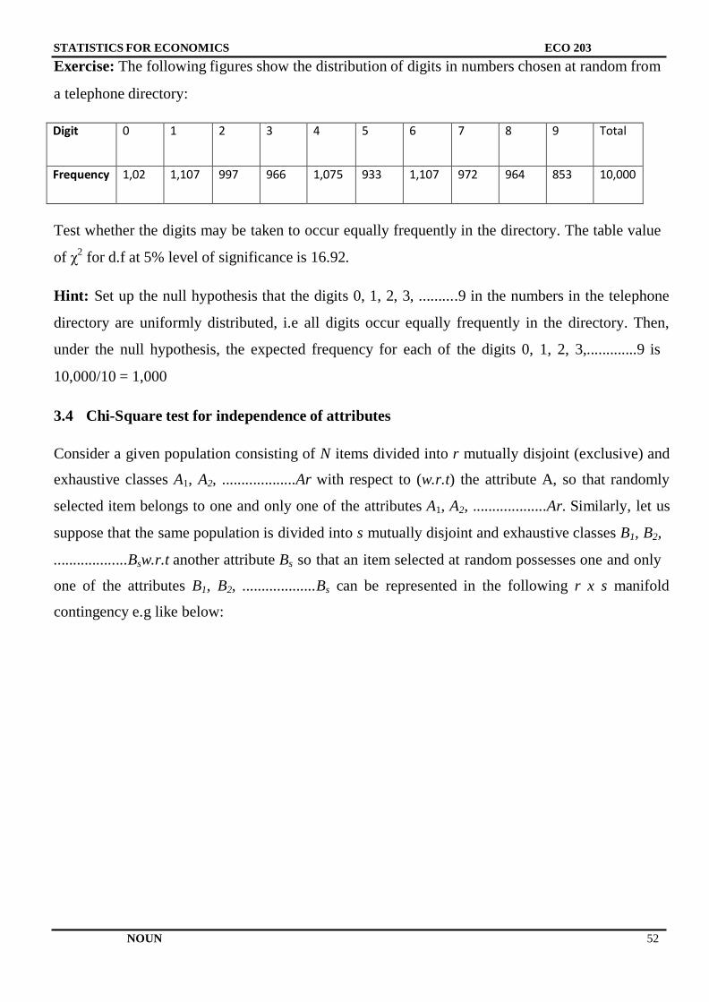
STATISTICS FOR ECONOMICS ECO 203
NOUN 52
Exercise: The following figures show the distribution of digits in numbers chosen at random from
a telephone directory:
Digit 0 1 2 3 4 5 6 7 8 9 Total
Frequency 1,02 1,107 997 966 1,075 933 1,107 972 964 853 10,000
Test whether the digits may be taken to occur equally frequently in the directory. The table value
of χ2
for d.f at 5% level of significance is 16.92.
Hint: Set up the null hypothesis that the digits 0, 1, 2, 3, ..........9 in the numbers in the telephone
directory are uniformly distributed, i.e all digits occur equally frequently in the directory. Then,
under the null hypothesis, the expected frequency for each of the digits 0, 1, 2, 3,.............9 is
10,000/10 = 1,000
3.4 Chi-Square test for independence of attributes
Consider a given population consisting of N items divided into r mutually disjoint (exclusive) and
exhaustive classes A1, A2, ...................Ar with respect to (w.r.t) the attribute A, so that randomly
selected item belongs to one and only one of the attributes A1, A2, ...................Ar. Similarly, let us
suppose that the same population is divided into s mutually disjoint and exhaustive classes B1, B2,
...................Bsw.r.t another attribute Bs so that an item selected at random possesses one and only
one of the attributes B1, B2, ...................Bs can be represented in the following r x s manifold
contingency e.g like below:
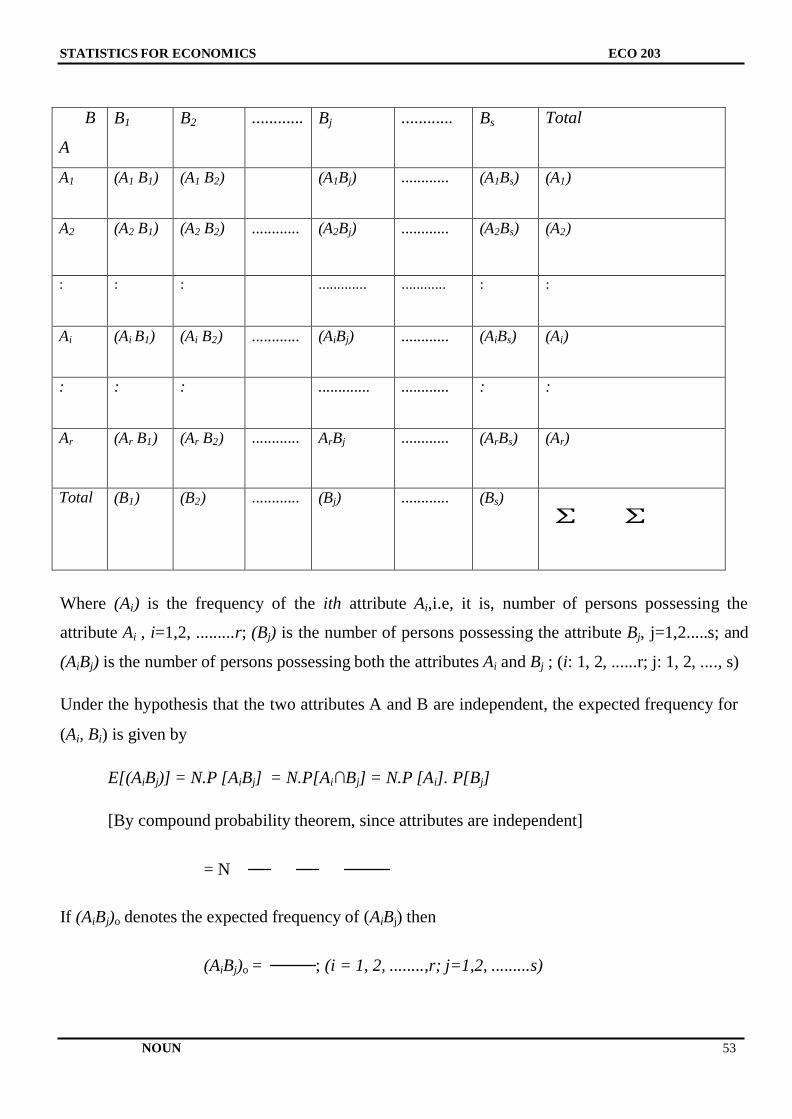
STATISTICS FOR ECONOMICS ECO 203
NOUN 53
B
A
B1 B2 ............ Bj ............ Bs Total
A1 (A1 B1) (A1 B2) (A1Bj) ............ (A1Bs) (A1)
A2 (A2 B1) (A2 B2) ............ (A2Bj) ............ (A2Bs) (A2)
: : : ............. ............ : :
Ai (Ai B1) (Ai B2) ............ (AiBj) ............ (AiBs) (Ai)
: : : ............. ............ : :
Ar (Ar B1) (Ar B2) ............ ArBj ............ (ArBs) (Ar)
Total (B1) (B2) ............ (Bj) ............ (Bs) ∑ ∑
Where (Ai) is the frequency of the ith attribute Ai,i.e, it is, number of persons possessing the
attribute Ai , i=1,2, .........r; (Bj) is the number of persons possessing the attribute Bj, j=1,2.....s; and
(AiBj) is the number of persons possessing both the attributes Ai and Bj ; (i: 1, 2, ......r; j: 1, 2, ...., s)
Under the hypothesis that the two attributes A and B are independent, the expected frequency for
(Ai, Bi) is given by
E[(AiBj)] = N.P [AiBj] = N.P[Ai∩Bj] = N.P [Ai]. P[Bj]
[By compound probability theorem, since attributes are independent]
= N
If (AiBj)o denotes the expected frequency of (AiBj) then
(AiBj)o = ; (i = 1, 2, ........,r; j=1,2, .........s)
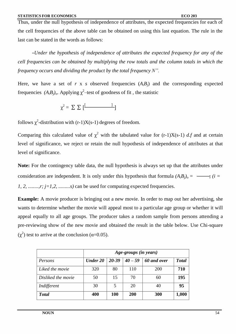
STATISTICS FOR ECONOMICS ECO 203
NOUN 54
Thus, under the null hypothesis of independence of attributes, the expected frequencies for each of
the cell frequencies of the above table can be obtained on using this last equation. The rule in the
last can be stated in the words as follows:
―Under the hypothesis of independence of attributes the expected frequency for any of the
cell frequencies can be obtained by multiplying the row totals and the column totals in which the
frequency occurs and dividing the product by the total frequency N”.
Here, we have a set of r x s observed frequencies (AiBj) and the corresponding expected
frequencies (AiBj)o. Applying χ2–test of goodness of fit , the statistic
χ2
= ∑ ∑ [[ ]
]
follows χ2-distribution with (r-1)X(s-1) degrees of freedom.
Comparing this calculated value of χ2
with the tabulated value for (r-1)X(s-1) d.f and at certain
level of significance, we reject or retain the null hypothesis of independence of attributes at that
level of significance.
Note: For the contingency table data, the null hypothesis is always set up that the attributes under
consideration are independent. It is only under this hypothesis that formula (AiBj)o = ; (i =
1, 2, ........,r; j=1,2, .........s) can be used for computing expected frequencies.
Example: A movie producer is bringing out a new movie. In order to map out her advertising, she
wants to determine whether the movie will appeal most to a particular age group or whether it will
appeal equally to all age groups. The producer takes a random sample from persons attending a
pre-reviewing show of the new movie and obtained the result in the table below. Use Chi-square
(χ2) test to arrive at the conclusion (α=0.05).
Age-groups (in years)
Persons Under 20 20-39 40 – 59 60 and over Total
Liked the movie 320 80 110 200 710
Disliked the movie 50 15 70 60 195
Indifferent 30 5 20 40 95
Total 400 100 200 300 1,000
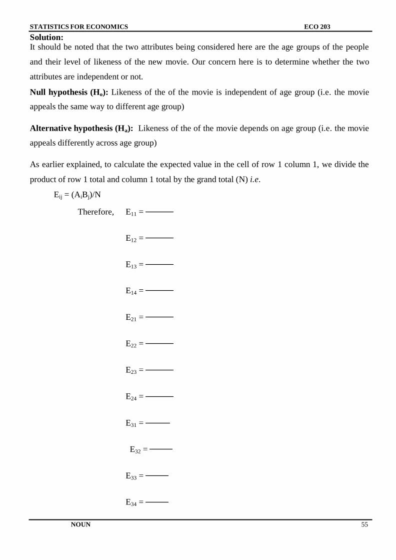
STATISTICS FOR ECONOMICS ECO 203
NOUN 55
Solution: It should be noted that the two attributes being considered here are the age groups of the people
and their level of likeness of the new movie. Our concern here is to determine whether the two
attributes are independent or not.
Null hypothesis (Ho): Likeness of the of the movie is independent of age group (i.e. the movie
appeals the same way to different age group)
Alternative hypothesis (Ha): Likeness of the of the movie depends on age group (i.e. the movie
appeals differently across age group)
As earlier explained, to calculate the expected value in the cell of row 1 column 1, we divide the
product of row 1 total and column 1 total by the grand total (N) i.e.
Eij = (AiBj)/N
Therefore, E11 =
E12 =
E13 =
E14 =
E21 =
E22 =
E23 =
E24 =
E31 =
E32 =
E33 =
E34 =
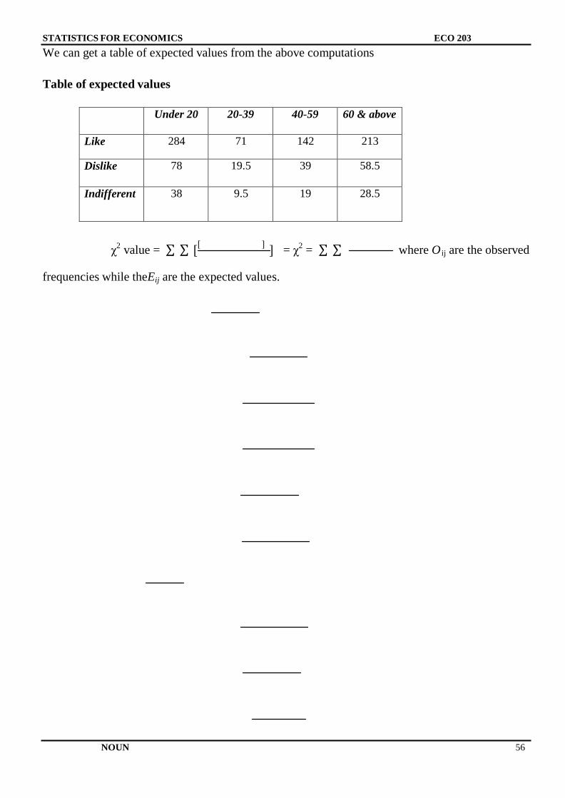
STATISTICS FOR ECONOMICS ECO 203
NOUN 56
ij
We can get a table of expected values from the above computations
Table of expected values
Under 20 20-39 40-59 60 & above
Like 284 71 142 213
Dislike 78 19.5 39 58.5
Indifferent 38 9.5 19 28.5
χ2
value = ∑ ∑ [[ ]
] = χ2
= ∑ ∑ where O
frequencies while theEij are the expected values.
are the observed
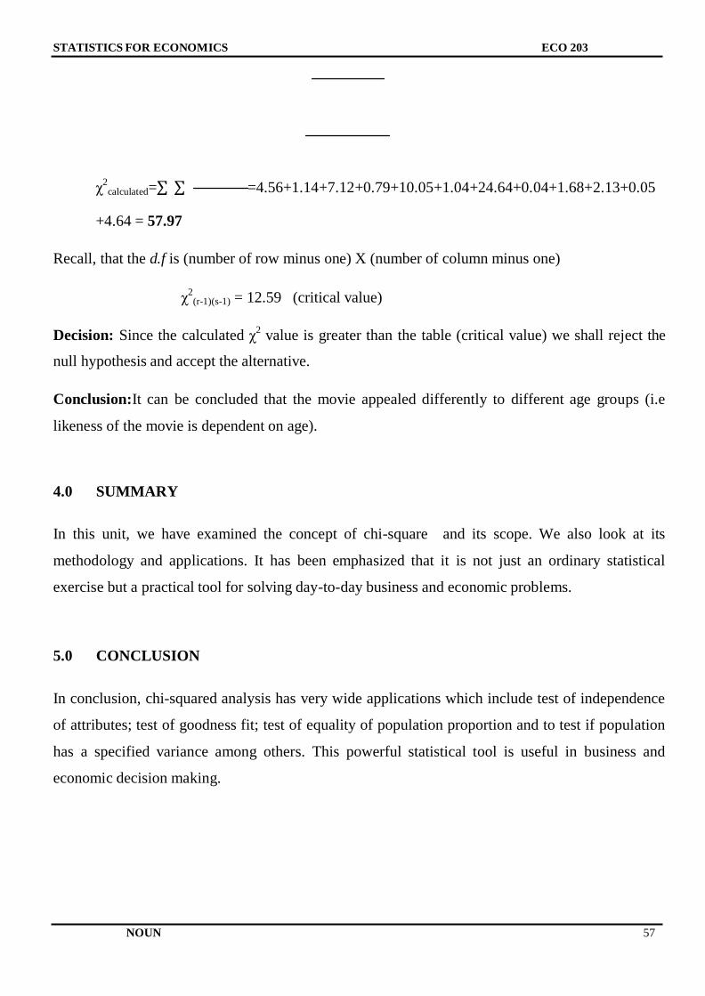
STATISTICS FOR ECONOMICS ECO 203
NOUN 57
χ2
calculated=∑ ∑ =4.56+1.14+7.12+0.79+10.05+1.04+24.64+0.04+1.68+2.13+0.05
+4.64 = 57.97
Recall, that the d.f is (number of row minus one) X (number of column minus one)
χ2
(r-1)(s-1) = 12.59 (critical value)
Decision: Since the calculated χ2
value is greater than the table (critical value) we shall reject the
null hypothesis and accept the alternative.
Conclusion:It can be concluded that the movie appealed differently to different age groups (i.e
likeness of the movie is dependent on age).
4.0 SUMMARY
In this unit, we have examined the concept of chi-square and its scope. We also look at its
methodology and applications. It has been emphasized that it is not just an ordinary statistical
exercise but a practical tool for solving day-to-day business and economic problems.
5.0 CONCLUSION
In conclusion, chi-squared analysis has very wide applications which include test of independence
of attributes; test of goodness fit; test of equality of population proportion and to test if population
has a specified variance among others. This powerful statistical tool is useful in business and
economic decision making.
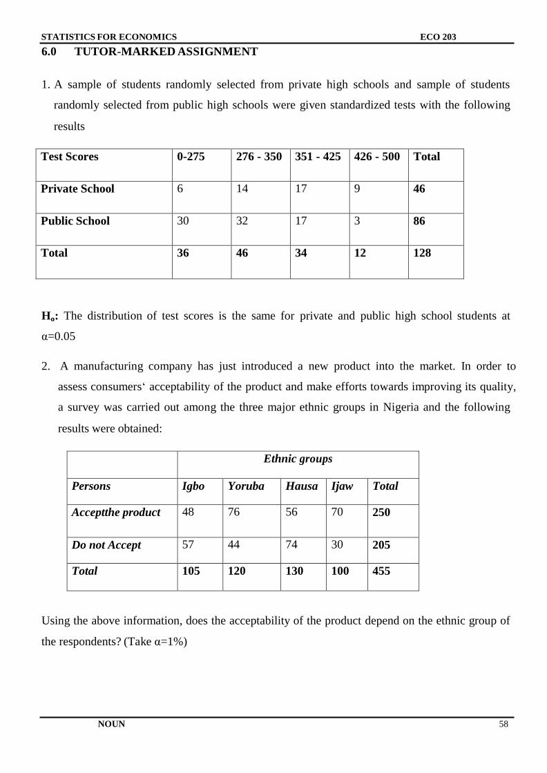
STATISTICS FOR ECONOMICS ECO 203
NOUN 58
6.0 TUTOR-MARKED ASSIGNMENT
1. A sample of students randomly selected from private high schools and sample of students
randomly selected from public high schools were given standardized tests with the following
results
Test Scores 0-275 276 - 350 351 - 425 426 - 500 Total
Private School 6 14 17 9 46
Public School 30 32 17 3 86
Total 36 46 34 12 128
Ho: The distribution of test scores is the same for private and public high school students at
α=0.05
2. A manufacturing company has just introduced a new product into the market. In order to
assess consumers‘ acceptability of the product and make efforts towards improving its quality,
a survey was carried out among the three major ethnic groups in Nigeria and the following
results were obtained:
Ethnic groups
Persons Igbo Yoruba Hausa Ijaw Total
Acceptthe product 48 76 56 70 250
Do not Accept 57 44 74 30 205
Total 105 120 130 100 455
Using the above information, does the acceptability of the product depend on the ethnic group of
the respondents? (Take α=1%)
STATISTICS FOR ECONOMICS ECO 203
NOUN 59
7.0 REFERENCES/FURTHER READING
Spiegel, M. R. and Stephens L. J. (2008).Statistics. (4th ed.). New York: McGraw Hill Press.
Gupta S.C. (2011). Fundamentals of Statistics. (6th Rev. and Enlarged ed.). Mumbai, India:
Himalayan Publishing House.
Swift L. (1997).Mathematics and Statistics for Business, Management and Finance. London:
Macmillan
STATISTICS FOR ECONOMICS ECO 203
NOUN 60
UNIT 4: ANALYSIS OF VARIANCE (ANOVA)
1.0 Objectives
2.0 Introduction
3.0 Main Content
3.1 Assumption for ANOVA test
3.2 The one-way classification
3.3 Bernoulli Distribution
4.0 Summary
5.0 Conclusion
6.0 Assignment
7.0 References/Further Reading
1.0 OBJECTIVE
The main objective of this unit is to teach students the theories and application of Analysis of
Variance (ANOVA). It is hoped that students should after taking this unit be able to apply
ANOVA in solving business and economic problem especially as it concern multiple comparison
of means
2.0 INTRODUCTION
In day-to-day business management and in sciences, instances may arise where we need to
compare means. If there are only two means e.g. average recharge card expenditure between male
and female students in a faculty of a University, the typical t-test for the difference of two means
becomes handy to solve this type of problem. However in real life situation man is always
confronted with situation where we need to compare more than two means at the same time. The
typical t-test for the difference of two means is not capable of handling this type of problem;
otherwise, the obvious method is to compare two means at a time by using the t-test earlier
treated. This process is very time consuming, since as few as 4 sample means would require 4C2 =
6, different tests to compare 6 possible pairs of sample means. Therefore, there must be a
procedure that can compare all means simultaneously. One such procedure is the analysis of
variance (ANOVA). For instance, we may be interested in the mean telephone recharge
STATISTICS FOR ECONOMICS ECO 203
NOUN 61
expenditures of various groups of students in the university such as student in the faculty of
Science, Arts, Social Sciences, Medicine, and Engineering. We may be interested in testing if the
average monthly expenditure of students in the five faculties are equal or not or whether they are
drawn from the same normal population. The answer to this problem is provided by the technique
of analysis of variance. It should be noted that the basic purpose of the analysis of variance is to
test the homogeneity of several means.
The term Analysis of Variance was introduced by Prof. R.A Fisher in 1920s to deal with problem
s in the analysis of agronomical data. Variation is inherent in nature. The total variation in any set
of numerical data is due to a number of causes which may be classified as:
(i) Assignable causes and (ii) chance causes
The variation due to assignable causes can be detected and measured whereas the variation due to
chances is beyond the control of human and cannot be traced separately.
3.0 MAIN CONTENT
3.1 Assumption for ANOVA test
ANOVA test is based on the test statistic F (or variance ratio). For the validity of the F-test in
ANOVA, the following assumption are made:
(i) The observations are independent.
(ii) Parent population from which observation are taken are normal.
(iii) Various treatment and environmental effects are additive in nature.
ANOVA as a tool has different dimensions and complexities. ANOVA can be (a) One-way
classification or (b) two-way classification. However, the one-way ANOVA will dealt with in this
course material
STATISTICS FOR ECONOMICS ECO 203
NOUN 62
Note
(i) ANOVA technique enables us to compare several population means simultaneously and
thus results in lot of saving in terms of time and money as compared to several
experiments required for comparing two populations means at a time.
(ii) The origin of the ANOVA technique lies in agricultural experiments and as such its
language is loaded with such terms as treatments, blocks, plots etc. However, ANOVA
technique is so versatile that it finds applications in almost all types of design of
experiments in various diverse fields such as industry, education, psychology, business,
economics etc.
(iii) It should be clearly understood that ANOVA technique is not designed to test equality
of several population variances. Rather, its objective is to test the equality of several
population means or the homogeneity of several independent sample means.
(iv) In addition to testing the homogeneity of several sample means, the ANOVA technique
is now frequently applied in testing the linearity of the fitted regression line or the
significance of the correlation ratio.
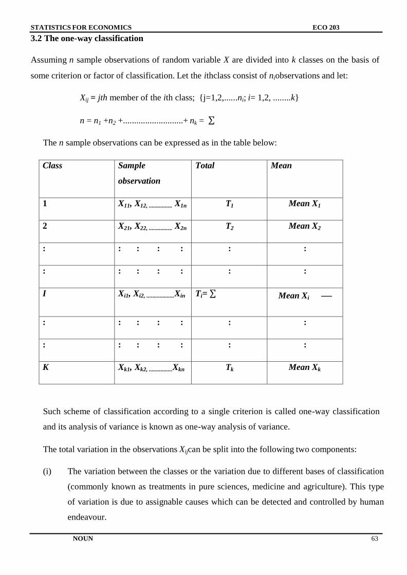
STATISTICS FOR ECONOMICS ECO 203
NOUN 63
3.2 The one-way classification
Assuming n sample observations of random variable X are divided into k classes on the basis of
some criterion or factor of classification. Let the ithclass consist of niobservations and let:
Xij = jth member of the ith class; {j=1,2,......ni; i= 1,2, ........k}
n = n1 +n2 +...........................+ nk = ∑
The n sample observations can be expressed as in the table below:
Class Sample
observation
Total Mean
1 X11, X12, ................ X1n T1 Mean X1
2 X21, X22, ................ X2n T2 Mean X2
: : : : : : :
: : : : : : :
I Xi1, Xi2, ...................Xin Ti= ∑
Mean Xi
: : : : : : :
: : : : : : :
K Xk1, Xk2, ................Xkn Tk Mean Xk
Such scheme of classification according to a single criterion is called one-way classification
and its analysis of variance is known as one-way analysis of variance.
The total variation in the observations Xijcan be split into the following two components:
(i) The variation between the classes or the variation due to different bases of classification
(commonly known as treatments in pure sciences, medicine and agriculture). This type
of variation is due to assignable causes which can be detected and controlled by human
endeavour.
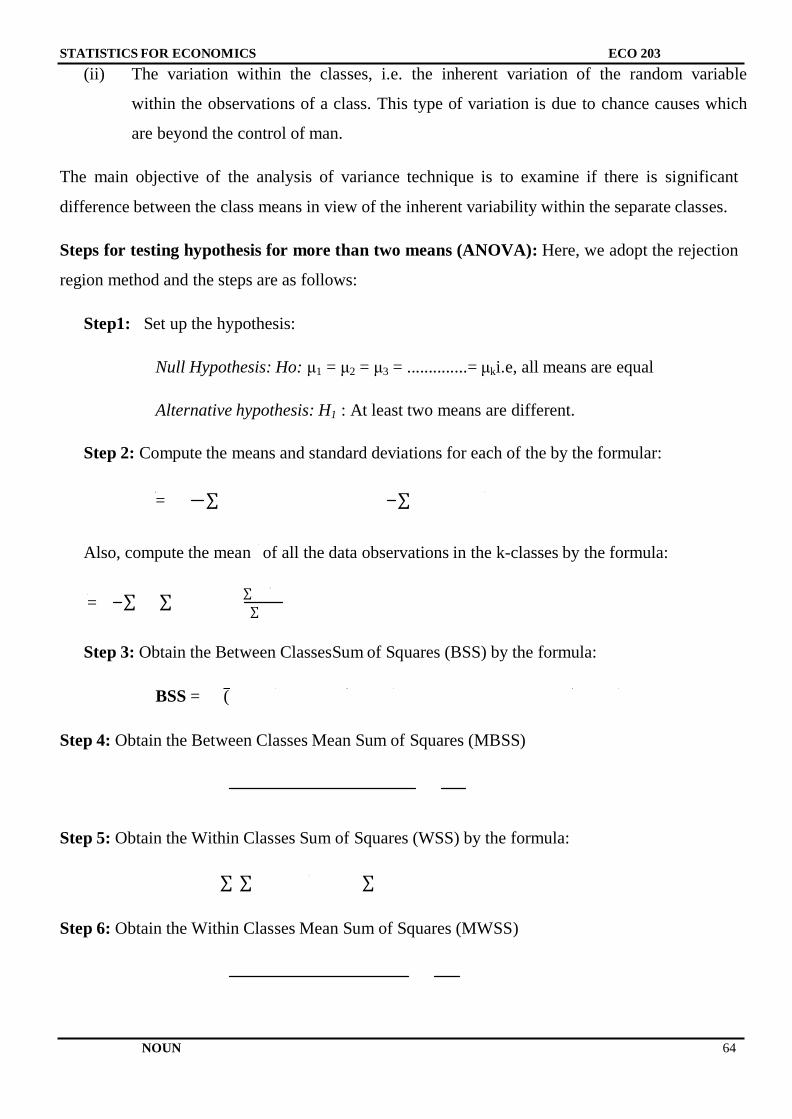
STATISTICS FOR ECONOMICS ECO 203
NOUN 64
(ii) The variation within the classes, i.e. the inherent variation of the random variable
within the observations of a class. This type of variation is due to chance causes which
are beyond the control of man.
The main objective of the analysis of variance technique is to examine if there is significant
difference between the class means in view of the inherent variability within the separate classes.
Steps for testing hypothesis for more than two means (ANOVA): Here, we adopt the rejection
region method and the steps are as follows:
Step1: Set up the hypothesis:
Null Hypothesis: Ho: μ1 = μ2 = μ3 = ..............= μki.e, all means are equal
Alternative hypothesis: H1 : At least two means are different.
Step 2: Compute the means and standard deviations for each of the by the formular:
= ∑ ∑
Also, compute the mean of all the data observations in the k-classes by the formula:
= ∑ ∑ ∑
∑
Step 3: Obtain the Between ClassesSum of Squares (BSS) by the formula:
BSS = (
Step 4: Obtain the Between Classes Mean Sum of Squares (MBSS)
Step 5: Obtain the Within Classes Sum of Squares (WSS) by the formula:
∑ ∑ ∑
Step 6: Obtain the Within Classes Mean Sum of Squares (MWSS)
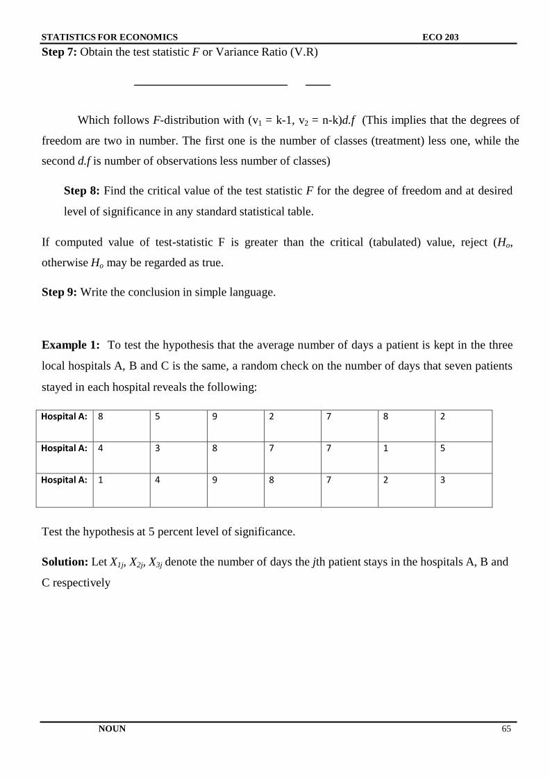
STATISTICS FOR ECONOMICS ECO 203
NOUN 65
Step 7: Obtain the test statistic F or Variance Ratio (V.R)
Which follows F-distribution with (v1 = k-1, v2 = n-k)d.f (This implies that the degrees of
freedom are two in number. The first one is the number of classes (treatment) less one, while the
second d.f is number of observations less number of classes)
Step 8: Find the critical value of the test statistic F for the degree of freedom and at desired
level of significance in any standard statistical table.
If computed value of test-statistic F is greater than the critical (tabulated) value, reject (Ho,
otherwise Ho may be regarded as true.
Step 9: Write the conclusion in simple language.
Example 1: To test the hypothesis that the average number of days a patient is kept in the three
local hospitals A, B and C is the same, a random check on the number of days that seven patients
stayed in each hospital reveals the following:
Hospital A: 8 5 9 2 7 8 2
Hospital A: 4 3 8 7 7 1 5
Hospital A: 1 4 9 8 7 2 3
Test the hypothesis at 5 percent level of significance.
Solution: Let X1j, X2j, X3j denote the number of days the jth patient stays in the hospitals A, B and
C respectively
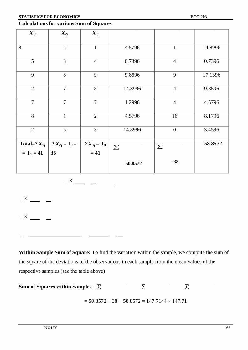
STATISTICS FOR ECONOMICS ECO 203
NOUN 66
Calculations for various Sum of Squares
X1j X2j X3j
8 4 1 4.5796 1 14.8996
5 3 4 0.7396 4 0.7396
9 8 9 9.8596 9 17.1396
2 7 8 14.8996 4 9.8596
7 7 7 1.2996 4 4.5796
8 1 2 4.5796 16 8.1796
2 5 3 14.8996 0 3.4596
Total=ƩX1j
= T1 = 41
ƩX2j = T2=
35
ƩX3j = T3
= 41
∑
=50.8572
∑
=38
=58.8572
= ∑
;
= ∑
= ∑
=
Within Sample Sum of Square: To find the variation within the sample, we compute the sum of
the square of the deviations of the observations in each sample from the mean values of the
respective samples (see the table above)
Sum of Squares within Samples = ∑ ∑ ∑
= 50.8572 + 38 + 58.8572 = 147.7144 ~ 147.71
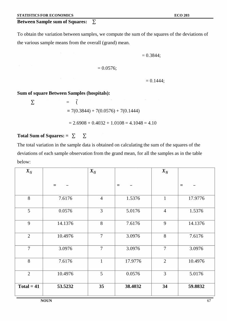
STATISTICS FOR ECONOMICS ECO 203
NOUN 67
Between Sample sum of Squares: ∑
To obtain the variation between samples, we compute the sum of the squares of the deviations of
the various sample means from the overall (grand) mean.
= 0.3844;
= 0.0576;
= 0.1444;
Sum of square Between Samples (hospitals):
∑ = (
= 7(0.3844) + 7(0.0576) + 7(0.1444)
= 2.6908 + 0.4032 + 1.0108 = 4.1048 = 4.10
Total Sum of Squares: = ∑ ∑
The total variation in the sample data is obtained on calculating the sum of the squares of the
deviations of each sample observation from the grand mean, for all the samples as in the table
below:
X1j
= –
X2j
= –
X3j
= –
8 7.6176 4 1.5376 1 17.9776
5 0.0576 3 5.0176 4 1.5376
9 14.1376 8 7.6176 9 14.1376
2 10.4976 7 3.0976 8 7.6176
7 3.0976 7 3.0976 7 3.0976
8 7.6176 1 17.9776 2 10.4976
2 10.4976 5 0.0576 3 5.0176
Total = 41 53.5232 35 38.4032 34 59.8832
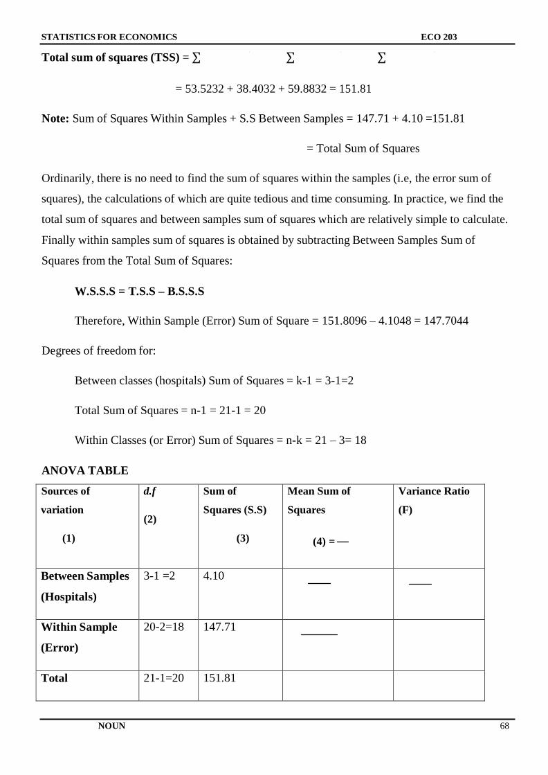
STATISTICS FOR ECONOMICS ECO 203
NOUN 68
Total sum of squares (TSS) = ∑ ∑ ∑
= 53.5232 + 38.4032 + 59.8832 = 151.81
Note: Sum of Squares Within Samples + S.S Between Samples = 147.71 + 4.10 =151.81
= Total Sum of Squares
Ordinarily, there is no need to find the sum of squares within the samples (i.e, the error sum of
squares), the calculations of which are quite tedious and time consuming. In practice, we find the
total sum of squares and between samples sum of squares which are relatively simple to calculate.
Finally within samples sum of squares is obtained by subtracting Between Samples Sum of
Squares from the Total Sum of Squares:
W.S.S.S = T.S.S – B.S.S.S
Therefore, Within Sample (Error) Sum of Square = 151.8096 – 4.1048 = 147.7044
Degrees of freedom for:
Between classes (hospitals) Sum of Squares = k-1 = 3-1=2
Total Sum of Squares = n-1 = 21-1 = 20
Within Classes (or Error) Sum of Squares = n-k = 21 – 3= 18
ANOVA TABLE
Sources of
variation
(1)
d.f
(2)
Sum of
Squares (S.S)
(3)
Mean Sum of
Squares
(4) =
Variance Ratio
(F)
Between Samples
(Hospitals)
3-1 =2 4.10
Within Sample
(Error)
20-2=18 147.71
Total 21-1=20 151.81
STATISTICS FOR ECONOMICS ECO 203
NOUN 69
Critical Value: The tabulated (critical) value of F for d.f (v1=2, v2=18) d.f at 5% level of
significance is 3.55
Since the calculated F = 0.25 is less than the critical value 3.55, it is not significant. Hence we fail
to accept Ho.
However, in cases like this when MSS between classes is less than the MSS within classes, we
need not calculate F and we may conclude that the means, , and do not differ
significantly. Hence, Ho may be regarded as true.
Conclusion: Ho : μ1 = μ2 = μ3, may be regarded as true and we may conclude that there is no
significant difference in the average stay at each of the three hospitals.
Critical Difference: If the classes (called treatments in pure sciences) show significant effect then
we would be interested to find out which pair(s) of treatment differs significantly. Instead of
calculating Student‘s t for different pairs of classes (treatments) means, we calculate the Least
Significant Difference (LSD) at the given level of significance. This LSD is also known as
Critical Difference (CD).
The LSD between any two classes (treatments) means, say and at level of significance ‗α‘ is
given by:
LSD ( - ) = [The critical value of t at level of significance α and error d.f] X [S.E ( - )]
Note: S.E means Standard Error. Therefore, the S.E ( - ) above mean the standard error of the
difference between the two means being considered.
= t n-k (α/2) X √
MSSE means sum of squares due to Error
If the difference | | between any two classes (treatments) means is greater than the LSD or
CD, it is said to be significant.
Another Method for the computation of various sums of squares
Step 1: Compute: G = ∑ ∑
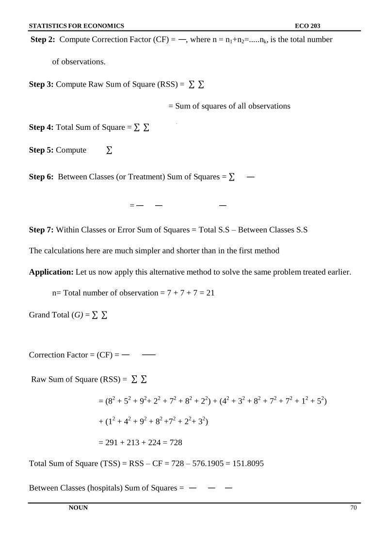
STATISTICS FOR ECONOMICS ECO 203
NOUN 70
Step 2: Compute Correction Factor (CF) = , where n = n1+n2=.....nk, is the total number
of observations.
Step 3: Compute Raw Sum of Square (RSS) = ∑ ∑
= Sum of squares of all observations
Step 4: Total Sum of Square = ∑ ∑
Step 5: Compute ∑
Step 6: Between Classes (or Treatment) Sum of Squares = ∑
=
Step 7: Within Classes or Error Sum of Squares = Total S.S – Between Classes S.S
The calculations here are much simpler and shorter than in the first method
Application: Let us now apply this alternative method to solve the same problem treated earlier.
n= Total number of observation = 7 + 7 + 7 = 21
Grand Total (G) = ∑ ∑
Correction Factor = (CF) =
Raw Sum of Square (RSS) = ∑ ∑
= (8
2 + 5
2 + 9
2+ 2
2 + 7
2 + 8
2 + 2
2) + (4
2 + 3
2 + 8
2 + 7
2 + 7
2 + 1
2 + 5
2)
+ (12
+ 42
+ 92
+ 82 +7
2 + 2
2+ 3
2)
= 291 + 213 + 224 = 728
Total Sum of Square (TSS) = RSS – CF = 728 – 576.1905 = 151.8095
Between Classes (hospitals) Sum of Squares =
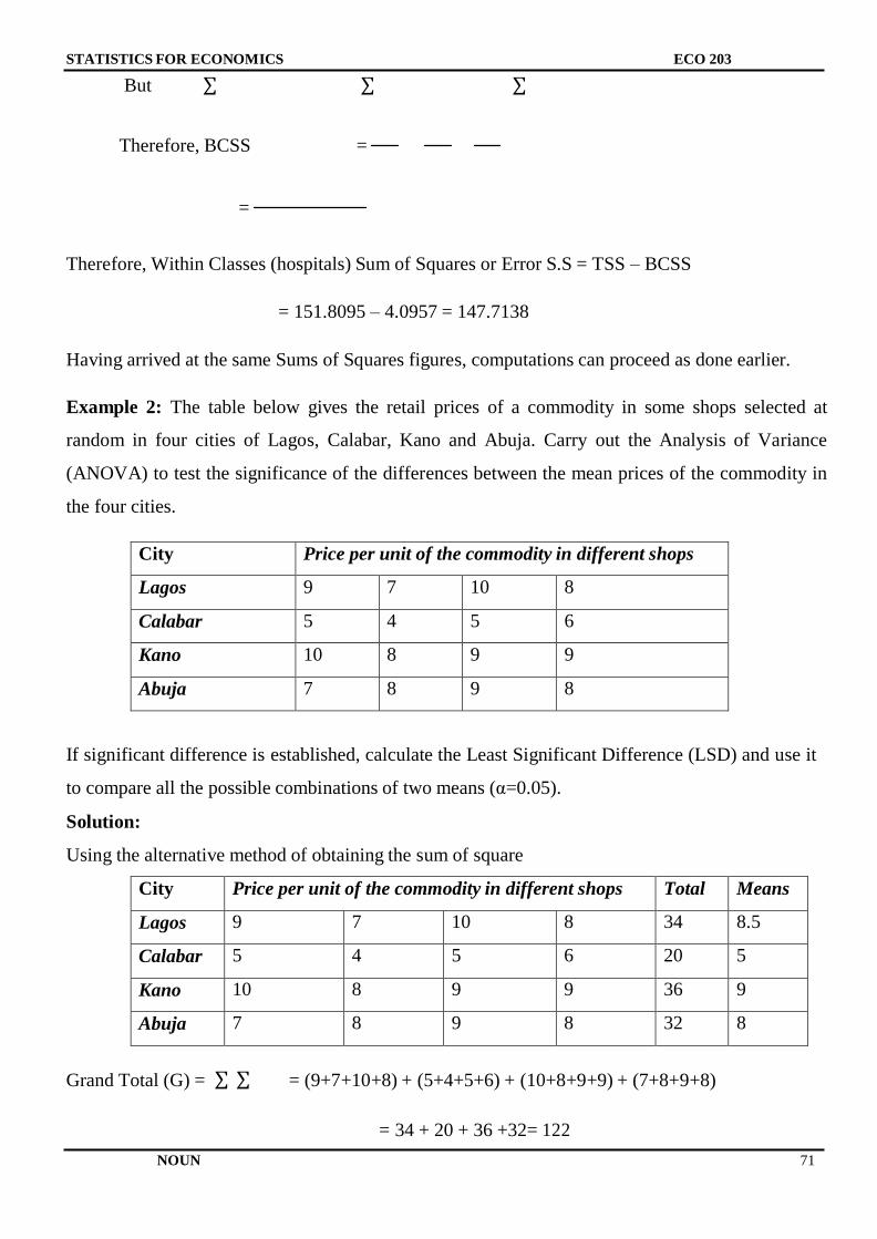
STATISTICS FOR ECONOMICS ECO 203
NOUN 71
But ∑ ∑ ∑
Therefore, BCSS =
=
Therefore, Within Classes (hospitals) Sum of Squares or Error S.S = TSS – BCSS
= 151.8095 – 4.0957 = 147.7138
Having arrived at the same Sums of Squares figures, computations can proceed as done earlier.
Example 2: The table below gives the retail prices of a commodity in some shops selected at
random in four cities of Lagos, Calabar, Kano and Abuja. Carry out the Analysis of Variance
(ANOVA) to test the significance of the differences between the mean prices of the commodity in
the four cities.
City Price per unit of the commodity in different shops
Lagos 9 7 10 8
Calabar 5 4 5 6
Kano 10 8 9 9
Abuja 7 8 9 8
If significant difference is established, calculate the Least Significant Difference (LSD) and use it
to compare all the possible combinations of two means (α=0.05).
Solution:
Using the alternative method of obtaining the sum of square
City Price per unit of the commodity in different shops Total Means
Lagos 9 7 10 8 34 8.5
Calabar 5 4 5 6 20 5
Kano 10 8 9 9 36 9
Abuja 7 8 9 8 32 8
Grand Total (G) = ∑ ∑ = (9+7+10+8) + (5+4+5+6) + (10+8+9+9) + (7+8+9+8)
= 34 + 20 + 36 +32= 122
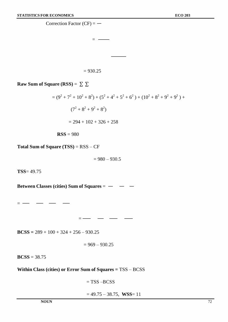
STATISTICS FOR ECONOMICS ECO 203
NOUN 72
Correction Factor (CF) =
=
= 930.25
Raw Sum of Square (RSS) = ∑ ∑
= (92
+ 72
+ 102
+ 82) + (5
2 + 4
2 + 5
2 + 6
2 ) + (10
2 + 8
2 + 9
2 + 9
2 ) +
(72
+ 82
+ 92
+ 82)
= 294 + 102 + 326 + 258
RSS = 980
Total Sum of Square (TSS) = RSS – CF
= 980 – 930.5
TSS= 49.75
Between Classes (cities) Sum of Squares =
=
=
BCSS = 289 + 100 + 324 + 256 – 930.25
= 969 – 930.25
BCSS = 38.75
Within Class (cities) or Error Sum of Squares = TSS – BCSS
= TSS –BCSS
= 49.75 – 38.75, WSS= 11
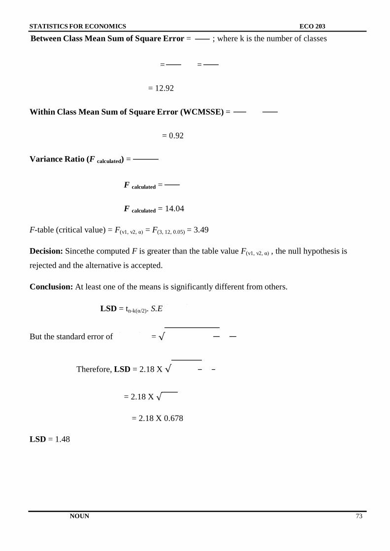
STATISTICS FOR ECONOMICS ECO 203
NOUN 73
Between Class Mean Sum of Square Error = ; where k is the number of classes
= =
= 12.92
Within Class Mean Sum of Square Error (WCMSSE) =
= 0.92
Variance Ratio (F calculated) =
F calculated =
F calculated = 14.04
F-table (critical value) = F(v1, v2, α) = F(3, 12, 0.05) = 3.49
Decision: Sincethe computed F is greater than the table value F(v1, v2, α) , the null hypothesis is
rejected and the alternative is accepted.
Conclusion: At least one of the means is significantly different from others.
LSD = tn-k(α/2). S.E
But the standard error of = √
Therefore, LSD = 2.18 X √
= 2.18 X √
= 2.18 X 0.678
LSD = 1.48
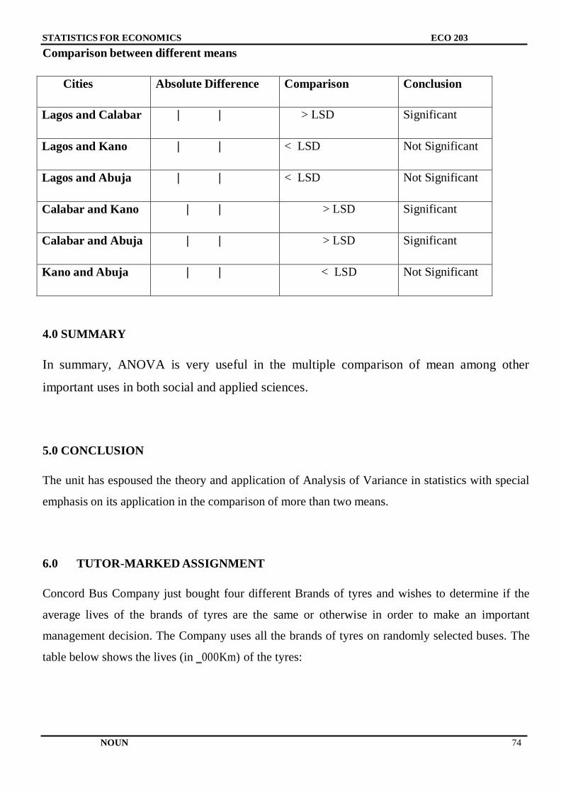
STATISTICS FOR ECONOMICS ECO 203
NOUN 74
Comparison between different means
Cities Absolute Difference Comparison Conclusion
Lagos and Calabar | |
> LSD Significant
Lagos and Kano | |
< LSD Not Significant
Lagos and Abuja | |
< LSD Not Significant
Calabar and Kano | |
> LSD Significant
Calabar and Abuja | |
> LSD Significant
Kano and Abuja | |
< LSD Not Significant
4.0 SUMMARY
In summary, ANOVA is very useful in the multiple comparison of mean among other
important uses in both social and applied sciences.
5.0 CONCLUSION
The unit has espoused the theory and application of Analysis of Variance in statistics with special
emphasis on its application in the comparison of more than two means.
6.0 TUTOR-MARKED ASSIGNMENT
Concord Bus Company just bought four different Brands of tyres and wishes to determine if the
average lives of the brands of tyres are the same or otherwise in order to make an important
management decision. The Company uses all the brands of tyres on randomly selected buses. The
table below shows the lives (in ‗000Km) of the tyres:
STATISTICS FOR ECONOMICS ECO 203
NOUN 75
Brand 1: 10, 12, 9, 9
Brand 2:
9,
8,
11,
8,
10
Brand 3:
11,
10,
10,
8,
7
Brand 4:
8,
9,
13,
9
Test the hypothesis that the average life for each of brand of tyres is the same. Take α = 0.01
7.0 REFERENCES/FURTHER READINGS
Spiegel, M. R. and Stephens L. J. (2008).Statistics. (4th ed.). New York: McGraw Hill Press.
Gupta S.C. (2011). Fundamentals of Statistics. (6th Rev. and Enlarged ed.). Mumbai, India:
Himalayan Publishing House.
Swift L. (1997).Mathematics and Statistics for Business, Management and Finance. London:
Macmillan
STATISTICS FOR ECONOMICS ECO 203
NOUN 76
UNIT 5: PARAMETRIC NON-PARAMETRIC TEST METHODS
CONTENTS
1.0 Objectives
2.0 Introduction
3.0 Main Content
4.0 Summary
5.0 Conclusion
6.0 Assignment
7.0 References/Further Reading
1.0 OBJECTIVES
The objective here is to explain to you that when our data is normally distributed, the mean is
equal to the median and we use the mean as our measure of centre. However, if our data is
skewed, then the median is a much better measure of centre. Therefore, just like the Z, t and F
tests made inferences about the population mean(s), nonparametric tests make inferences about
the population median(s).
2.0 INTRODUCTION
In statistics, the term non-parametric statistics refers to statistics that do not assume the data or
population have any characteristic structure or parameters. For example, non-parametric statistics
are suitable for examining the order in which runners complete a race, while parametric statistics
would be more appropriate for looking at the actual race times (which may possess parameters
such as a mean and standard deviation). In other words, the order (or "rank") of the values is used
rather than the actual values themselves.
In statistics, the term non-parametric statistics has at least two different meanings:
(1) The first meaning of non-parametric covers techniques that do not rely on data belonging to
any particular distribution. These include, among others:
STATISTICS FOR ECONOMICS ECO 203
NOUN 77
(a) distribution free methods, which do not rely on assumptions that the data are drawn from a
given probability distribution. As such it is the opposite of parametric statistics. It includes
non-parametric descriptive statistics, statistical models, inference and statistical tests.
(b) non-parametric statistics (in the sense of a statistic over data, which is defined to be a function
on a sample that has no dependency on a parameter), whose interpretation does not depend on
the population fitting any parameterised distributions. Order statistics, which are based on the
ranks of observations, are one example of such statistics and these play a central role in many
non-parametric approaches.
(2) The second meaning of non-parametric covers techniques that do not assume that the
structure of a model is fixed. Typically, the model grows in size to accommodate the
complexity of the data. In these techniques, individual variables are typically assumed to
belong to parametric distributions, and assumptions about the types of connections among
variables are also made. These techniques include, among others:
(a) non-parametric regression, which refers to modeling where the structure of the relationship
between variables is treated non-parametrically, but where nevertheless there may be
parametric assumptions about the distribution of model residuals.
(b) non-parametric hierarchical Bayesian models, such as models based on the Dirichlet process,
which allow the number of latent variables to grow as necessary to fit the data, but here
individual variables still follow parametric distributions and even the process controlling the
rate of growth of latent variables follows a parametric distribution.
3.0 MAIN CONTENT
Non-parametric methods are widely used for studying populations that take on a ranked order
(such as movie reviews receiving one to four stars). The use of non-parametric methods may be
necessary when data have a ranking but no clear numerical interpretation, such as when assessing
preferences. In terms of levels of measurement, non-parametric methods result in "ordinal" data.
As non-parametric methods make fewer assumptions, their applicability is much wider than the
corresponding parametric methods. In particular, they may be applied in situations where less is
STATISTICS FOR ECONOMICS ECO 203
NOUN 78
known about the application in question. Also, due to the reliance on fewer assumptions, non-
parametric methods are more robust.
Another justification for the use of non-parametric methods is simplicity. In certain cases, even
when the use of parametric methods is justified, non-parametric methods may be easier to use.
Due both to this simplicity and to their greater robustness, non-parametric methods are seen by
some statisticians as leaving less room for improper use and misunderstanding.
The wider applicability and increased robustness of non-parametric tests comes at a cost: in cases
where a parametric test would be appropriate, non-parametric tests have less power. In other
words, a larger sample size can be required to draw conclusions with the same degree of
confidence.
Non-parametric models differ from parametric models in that the model structure is not
specified a priori but is instead determined from data. The term non-parametricis not meant to
imply that such models completely lack parameters but that the number and nature of the
parameters are flexible and not fixed in advance.
Non-parametric (or distribution-free) inferential statistical methods are mathematical
procedures for statistical hypothesis testing which, unlike parametric statistics, make no
assumptions about the probability distributions of the variables being assessed. The most
frequently used tests include
1. Kruskal-Wallis one-way analysis of variance by ranks: tests whether >2 independent
samples are drawn from the same distribution
2. Spearman's rank correlation coefficient: measures statistical dependence between two
variables using a monotonic function
3. Sign test: tests whether matched pair samples are drawn from distributions with equal
medians
4. Wilcoxon signed-rank test: tests whether matched pair samples are drawn from populations
with different mean ranks
5. Mann–Whitney U or Wilcoxon rank sum test: tests whether two samples are drawn from
the same distribution, as compared to a given alternative hypothesis
6. Anderson–Darling test: tests whether a sample is drawn from a given distribution
STATISTICS FOR ECONOMICS ECO 203
NOUN 79
7. Statistical Bootstrap Methods: estimates the accuracy/sampling distribution of a statistic
8. Cochran's Q: tests whether k treatments in randomized block designs with 0/1 outcomes
have identical effects
9. Cohen's kappa: measures inter-rater agreement for categorical items
10. Friedman two-way analysis of variance by ranks: tests whether k treatments in randomized
block designs have identical effects
11. Kaplan–Meier: estimates the survival function from lifetime data, modelling censoring
12. Kendall's tau: measures statistical dependence between two variables
13. Kendall's W: a measure between 0 and 1 of inter-rater agreement
14. Kolmogorov–Smirnov test: tests whether a sample is drawn from a given distribution, or
whether two samples are drawn from the same distribution
15. Kuiper's test: tests whether a sample is drawn from a given distribution, sensitive to cyclic
variations such as day of the week
16. Logrank Test: compares survival distributions of two right-skewed, censored samples
17. McNemar's test: tests whether, in 2 × 2 contingency tables with a dichotomous trait and
matched pairs of subjects, row and column marginal frequencies are equal
18. Median test: tests whether two samples are drawn from distributions with equal medians
19. Pitman's permutation test: a statistical significance test that yields exact p values by
examining all possible rearrangements of labels
20. Rank products: detects differentially expressed genes in replicated microarray experiments
21. Siegel–Tukey test: tests for differences in scale between two groups
22. Squared ranks test: tests equality of variances in two or more samples
23. Wald–Wolfowitz runs test: tests whether the elements of a sequence are mutually
independent/random
1. The Sign Test
Suppose we are interested in testing
Ho: P(+) = P (-)
H1: P(+) ≠ P(-)
We shall require the following:
(i) +‘s and –‗s
STATISTICS FOR ECONOMICS ECO 203
NOUN 80
(ii) n = number of +‘s and –‗s
(iii) T number of +‘s
If T ≥ n-t, we shall reject Ho
Note always that P = ½. To get t, we look at value close to our α e.g. let α = 0.05, we look at value
closer to this value, the value on the left hand side of the table corresponding to this is our t. i.e.
the value under the column of P=0.5 in the Binomial Distribution table.
Example 1:
From the following information, test:
Ho: P(+) = P (-)
H1: P(+) ≠ P(-)
Number of +‘s = 8
Number of –‗s =1
Number of ties =1
Solution:
n = number of +‘s and –‗s =9
T = number of +‘s = 8
We now go into the Binomial distribution table with P= ½ (i.e. under the column of 0.50), n =9
and we look for value close to 0.05 but not more than. In this case, what we have is 0.0195. This
corresponds to 1. i.e. t=1.
Therefore, we reject Ho if
T ≥ n-t
T = 8, n=9, t =1
Therefore, 8 ≥ 9-1
8 = 8
Hence, we reject the null hypothesis
STATISTICS FOR ECONOMICS ECO 203
NOUN 81
Example 2: The following are measurements of the households‘ weekly demand for water in
litres: 163, 165, 160, 189, 161, 171, 158, 151, 169, 162, 163, 139, 172, 165, 148, 166, 172, 163,
187, 173.
Test the null hypothesis
μ = 160 against the alternative μ > 160 at α = 0.05
Solution:
Ho: μ = 160
H1: μ > 160
Critical region: Reject Ho
if T ≥ n-t Where T =
number of +‘s
Computations:
Replace each value exceeding 160with a plus sign, each value less than 160 with a negative sign
and discarding those actually equal to 160, we have the following:
+ + + + + - - + + + - + + - + + + + +
n = 19 (+‘s and –‗s added)
T = 15 (+‘s signs)
From the Binomial table, with n=19, P= 0.5, look for the value very close to α = 0.05, (say α1)
Therefore, α1 = 0.0318, it corresponds t= 5
Therefore, n-t = 19-5 = 14
Since T > n-t
i.e. 15 > 14 we therefore reject the null hypothesis
STATISTICS FOR ECONOMICS ECO 203
NOUN 82
Tests Based on Runs
A run is a succession of identical letters (or other kinds of symbol) which is preceded and
followed by different letters or no letters at all. E.g. consider the following:
M F M MM F FF M F M F M MM F F M MM
In the above example, there are 11 runs and they are represented by u i.e.
u = 11
n1 = 12 (for m‘s)
n2 = 8 (for F‘s)
When n1 and n2 are small, tests of the null hypothesis of randomness are usually based on
specially constructed tables in the any statistical tables. However, when n1 and n2 are either 10 or
more, the sampling distribution of u (the total number of Runs) can be approximated with a
normal distribution. For this, we require the following results:
E(u) =
Var (u) =
√
Use (- ½ ) when u> E(u)
and (+ ½) when u < E(u)
Example: Consider the following: nnnnnddddnnnnnnnnnnddnndddd n ddnn. Test the null
hypothesis of randomness at α = 1%.
Solution:
Ho: arrangement is random
H1: arrangement is not random
Critical region is -2.58 to 2.58
STATISTICS FOR ECONOMICS ECO 203
NOUN 83
Where √
Computation:
n1 = 20 (for n‘s)
n2 = 12 (for d‘s)
U = 9 (total number of runs)
E(u) =
=
= 16
E(9) < E(u) (16), hence we use + ½
Var (u) =
=
= 6.77
√
= -2.50
Decision: Since Z = -2.50 falls between -2.58 and 2.58, then we cannot reject the null hypothesis
of randomness.
The H-Test or the Kruskal-Wallis Test
This is a non-parametric test alternative to the one-way analysis of variance. The data are ranked
jointly from the smallest to the highest as though they constitute on sample. Then, letting Ri be the
sum of the ranks of the values in the ith sample, the test is based on the statistic:
∑
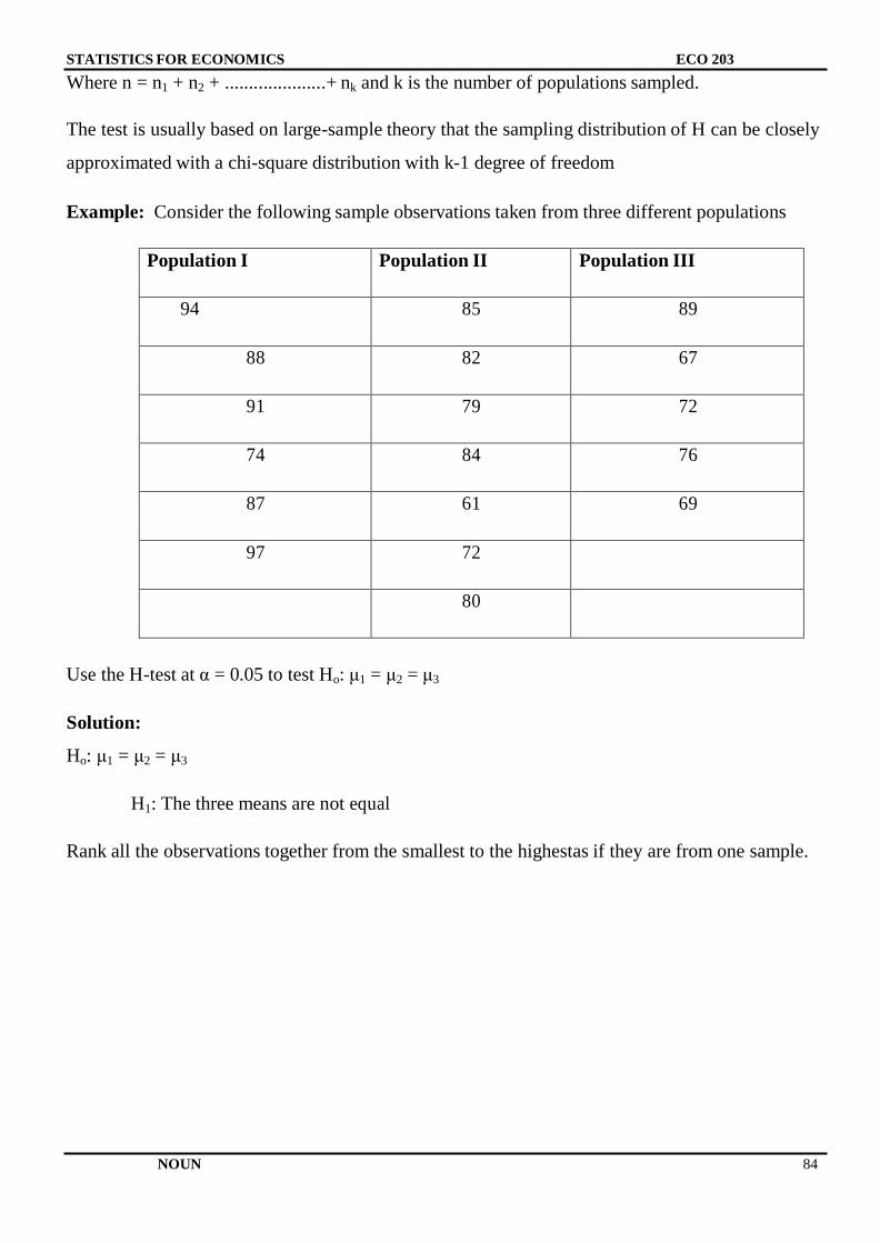
STATISTICS FOR ECONOMICS ECO 203
NOUN 84
Where n = n1 + n2 + .....................+ nk and k is the number of populations sampled.
The test is usually based on large-sample theory that the sampling distribution of H can be closely
approximated with a chi-square distribution with k-1 degree of freedom
Example: Consider the following sample observations taken from three different populations
Population I Population II Population III
94 85 89
88 82 67
91 79 72
74 84 76
87 61 69
97 72
80
Use the H-test at α = 0.05 to test Ho: μ1 = μ2 = μ3
Solution:
Ho: μ1 = μ2 = μ3
H1: The three means are not equal
Rank all the observations together from the smallest to the highestas if they are from one sample.
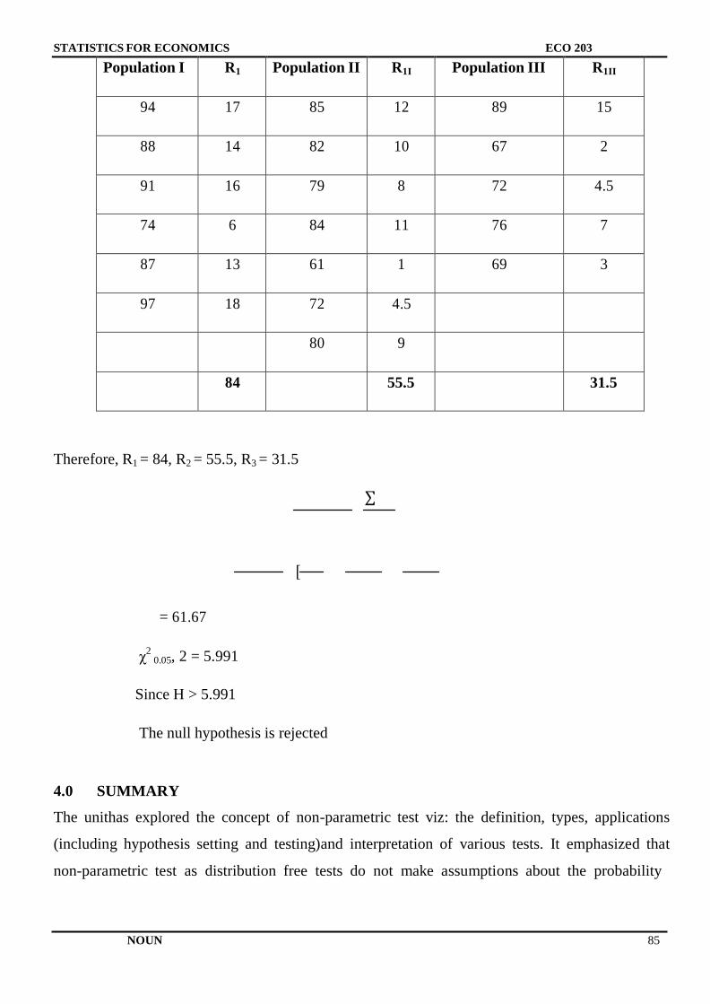
STATISTICS FOR ECONOMICS ECO 203
NOUN 85
Population I R1 Population II R1I Population III R1II
94 17 85 12 89 15
88 14 82 10 67 2
91 16 79 8 72 4.5
74 6 84 11 76 7
87 13 61 1 69 3
97 18 72 4.5
80 9
84 55.5 31.5
Therefore, R1 = 84, R2 = 55.5, R3 = 31.5
∑
[
= 61.67
χ2
0.05, 2 = 5.991
Since H > 5.991
The null hypothesis is rejected
4.0 SUMMARY
The unithas explored the concept of non-parametric test viz: the definition, types, applications
(including hypothesis setting and testing)and interpretation of various tests. It emphasized that
non-parametric test as distribution free tests do not make assumptions about the probability
STATISTICS FOR ECONOMICS ECO 203
NOUN 86
distributions of the variables being assessed. This also contributes to its flexibility and wide
applicability.
5.0 CONCLUSION
In conclusion, various forms of Non-Parametric Test exist which may fit perfectly well into
solving some qualitative problems which ordinarily may be difficult to solve with the
conventional parametric test. The diversity of the different methods available reflects the varieties
of problems they can solve.
6.0 TUTOR-MARKED ASSIGNMENT
1. Eighteen individuals were asked if the prefer apple juice to orange juice and the following
responses were obtained. Y YYY N N Y N Y YYY N Y N Y N Y (Y= Yes, N = No). Use the
sign test to test the null hypothesis
Ho: P(+) = P (-) against
H1: P(+) ≠ P(-) given that α = 0.05
2. Given YY N Y NN Y N YYYY N Y N Y N Y NNN YY N YYYY NN. Test the null
hypothesis of randomness at α = 1%
3. The weights (in Kilogrammes) of randomly selected students from four different arms of a class
were taken and the following results were obtained:

STATISTICS FOR ECONOMICS ECO 203
NOUN 87
A B C D
45 30 34 57
39 52 40 60
48 49 41 48
54 46 49 52
36 39 45 51
53 43 32 49
52 44 30 50
47 54 31 59
50 40 35 56
46 51 43
51 34
38
Use the H-test at α=0.05 to test equality of the four means.
7.0 REFERENCES/FURTHER READINGS
Gupta S.C (2011). Fundamentals of Statistics,(6th
Rev. and Enlarged ed.). Mumbai,
India:Himalayan Publishing House
FisherR. A. (1925).Statistical Methods for Research Workers, Edinburgh: Oliver and Boyd, p.43.
STATISTICS FOR ECONOMICS ECO 203
NOUN 88
MODULE 3: CORRELATION AND REGRESSION ANALYSIS
Correlation provides an estimate of the relationship between two measurements, without any
assumption of whether one comes before the other. For example, muscle mass and fat mass are
correlated, both depends on body size. Correlation coefficients have a value between -1 and +1. A
positive coefficient means that x and y values increases and decrease in the same direction. A
negative correlation means that as x and y move in opposite directions, one increases as the other
decreases. Coefficient of 0 means x and y are associated randomly.
The correlation measures only the degree of linear association between two variables
whileregression analysis is a statistical process for estimating the relationships among variables.
In this module the under listed topics will be considered:
Unit 1: Pearson’s Correlation Coefficient
Unit 2: Spearman’s Rank Correlation Coefficient
Unit 3: Methods of Curve and Eye Fitting of Scattered Plot
Unit 4: The Least Square Regression Line
Unit 5: Forecasting in Regression
UNIT 1: PEARSON’S CORRELATION
CONTENTS
1.0 Objectives
1.1 Introduction
3.0 Main Content
4.0 Summary
5.0 Conclusion
6.0 Tutor-Marked Assignment
7.0 References/Further Reading
STATISTICS FOR ECONOMICS ECO 203
NOUN 89
1.0 OBJECTIVES
The objectives for performing a Pearson Correlation Analysis are:
1. To discover whether there is a relationship between variables,
2. To find out the direction of the relationship – whether it is positive, negative or zero,
3. To find the strength of the relationship between the two variables
2.0 INTRODUCTION
For Pearson's correlation coefficient is based on pairs of measurement (x,y) and the data is entered
in 2 columns, each pair in a row. The coefficients, and whether it significantly differs from null
(0), are usually presented. More recently, the 95% confidence interval of the coefficient is
presented, and correlation can be considered statistically significant if the 95% confidence interval
does not overlap the zero (0) value. Sample size calculations or tables can be used for estimating
sample size requirements or power of the results in correlation.
3.0 MAIN CONTENT
Types of correlation
(a) Positive Correlation: Situations may arise when the values of two variables deviate in the
same direction i.e. if the increase in the values of one variables results, on an average, in a
corresponding increase in the values of the other variable or if a decrease in the values of one
variable results, on an average, in a corresponding decrease in the values of the other variable.
Correlation is said to be positive. Some examples of possible positive correlations are:
- Price and supply of a commodity
- Household income and demand for luxury items
- Height and Weight
- Rainfall and Farm yield
STATISTICS FOR ECONOMICS ECO 203
NOUN 90
(b) Negative Correlation: Correlation is said to be negative or inverse if the variables deviate
in the opposite direction i.e.; if the increase (or decrease) in the values of one variable
results, on the average, in a corresponding decrease (or increase) in the value of the other
variable. Example of negative correlation are:
- Quantity demanded and price
- Tax rate and consumption demand
(c) Linear Correlation: This describes a situation where for a unit change in one variable
there is a constant corresponding change in the other variable over the entire range of
values. E.g.
x: 1 2 3 4 5
y:2 5 8 11 14
As seen above, for a unit change in x, there is a constant change (i.e. 3) in the
corresponding value of y. This can be expressed as y = 2+3x
I general two variables are said to be linearly related if they have a relationship of the form
y = a+bx
(d) Non-linear or curvilinear correlation: This describes situations if corresponding to a unit
change one variable; the other variable does not change at a constant rate but at a
fluctuating rate.
Reasons for high correlation between two variables
(a) Mutual dependence: This is the situation when the phenomena under study inter-influence
each other. Such instances are usually observed in data relating to economic and business
situations.
(b) Both variables being influenced by the same external factor(s): A high degree of
correlation between the two variables may be due to the effect or interaction of a third
variable or a number of variables on each of these two variables.
(c) Chance: It may happen that a small randomly selected sample from a bivariate distribution
may show a fairly high degree of correlation though, actually, the variables may not be
correlated in the population. Such correlation may be due to chance fluctuation. For
STATISTICS FOR ECONOMICS ECO 203
NOUN 91
example, one may observe a high degree of correlation between the height and intelligence
in a group of people. Such correlation is called spurious or non-sense correlation.
Some Methods of Studying Correlation
1. Scatter Diagram method
2. Karl Pearson‘s coefficient of correlation
3. Edward Spearman Rank correlation method etc.
Interpretation of the value of r
Given two variables X and Y:
If r = +1, there is a perfect direct relationship between Y and X.
If r = -1, there is a perfect inverse or negative relationship between Y and X.
If r = 0, there is no relationship between Y and X.
Karl Pearson’s Correlation Method
Karl Pearson (1867 – 1936), was a British Biometrician and statistician suggested a mathematical
method for measuring the magnitude of linear relationship between two variables. Karl Pearson‘s
method, also known as Pearsonian correlation between two variables (series) X and Y, usually
denoted by r(X,Y) or rxy or ρ and it is given as:
∑ ∑ ∑
ρ = √[ ∑ ∑ ][ ∑ ∑ ]
Alternative formula that relies on deviation of each individual observation from the mean is also
frequently used where the deviation from the mean x = X- and y = Y- . Here and are the
sample means of the set of data Xi and Yi respectively. This formula is given as
∑
√∑ ∑
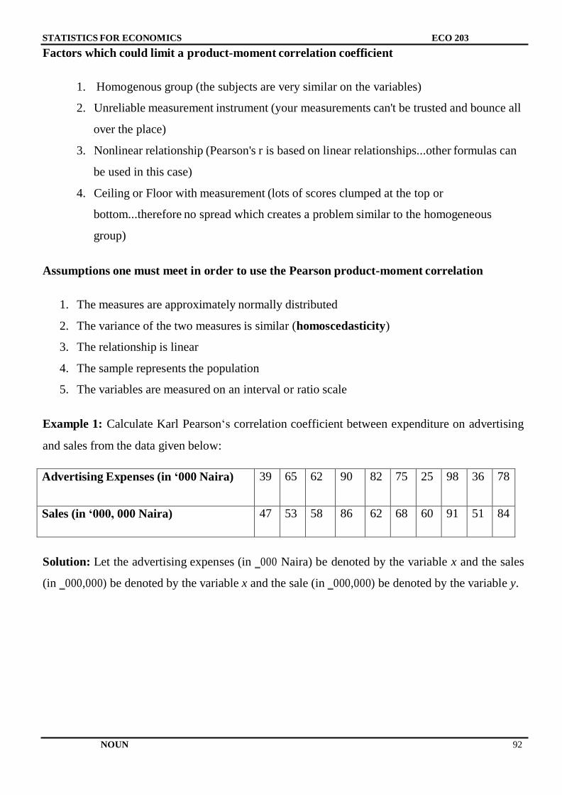
STATISTICS FOR ECONOMICS ECO 203
NOUN 92
Factors which could limit a product-moment correlation coefficient
1. Homogenous group (the subjects are very similar on the variables)
2. Unreliable measurement instrument (your measurements can't be trusted and bounce all
over the place)
3. Nonlinear relationship (Pearson's r is based on linear relationships...other formulas can
be used in this case)
4. Ceiling or Floor with measurement (lots of scores clumped at the top or
bottom...therefore no spread which creates a problem similar to the homogeneous
group)
Assumptions one must meet in order to use the Pearson product-moment correlation
1. The measures are approximately normally distributed
2. The variance of the two measures is similar (homoscedasticity)
3. The relationship is linear
4. The sample represents the population
5. The variables are measured on an interval or ratio scale
Example 1: Calculate Karl Pearson‘s correlation coefficient between expenditure on advertising
and sales from the data given below:
Advertising Expenses (in ‘000 Naira) 39 65 62 90 82 75 25 98 36 78
Sales (in ‘000, 000 Naira) 47 53 58 86 62 68 60 91 51 84
Solution: Let the advertising expenses (in ‗000 Naira) be denoted by the variable x and the sales
(in ‗000,000) be denoted by the variable x and the sale (in ‗000,000) be denoted by the variable y.
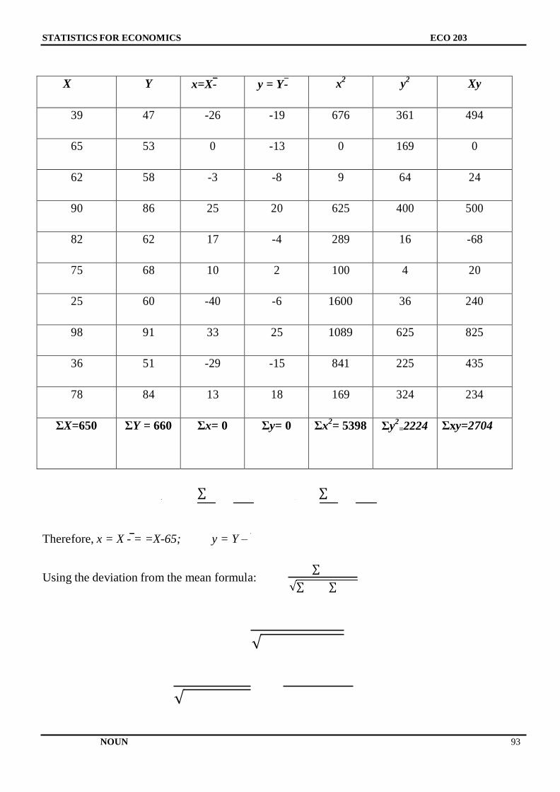
STATISTICS FOR ECONOMICS ECO 203
NOUN 93
X Y x=X-
y = Y-
x2 y
2 Xy
39 47 -26 -19 676 361 494
65 53 0 -13 0 169 0
62 58 -3 -8 9 64 24
90 86 25 20 625 400 500
82 62 17 -4 289 16 -68
75 68 10 2 100 4 20
25 60 -40 -6 1600 36 240
98 91 33 25 1089 625 825
36 51 -29 -15 841 225 435
78 84 13 18 169 324 234
ΣX=650 ΣY = 660 Σx= 0 Σy= 0 Σx2= 5398 Σy
2=2224 Σxy=2704
∑ ∑
Therefore, x = X - = =X-65; y = Y –
Using the deviation from the mean formula: ∑
√∑ ∑
√
√
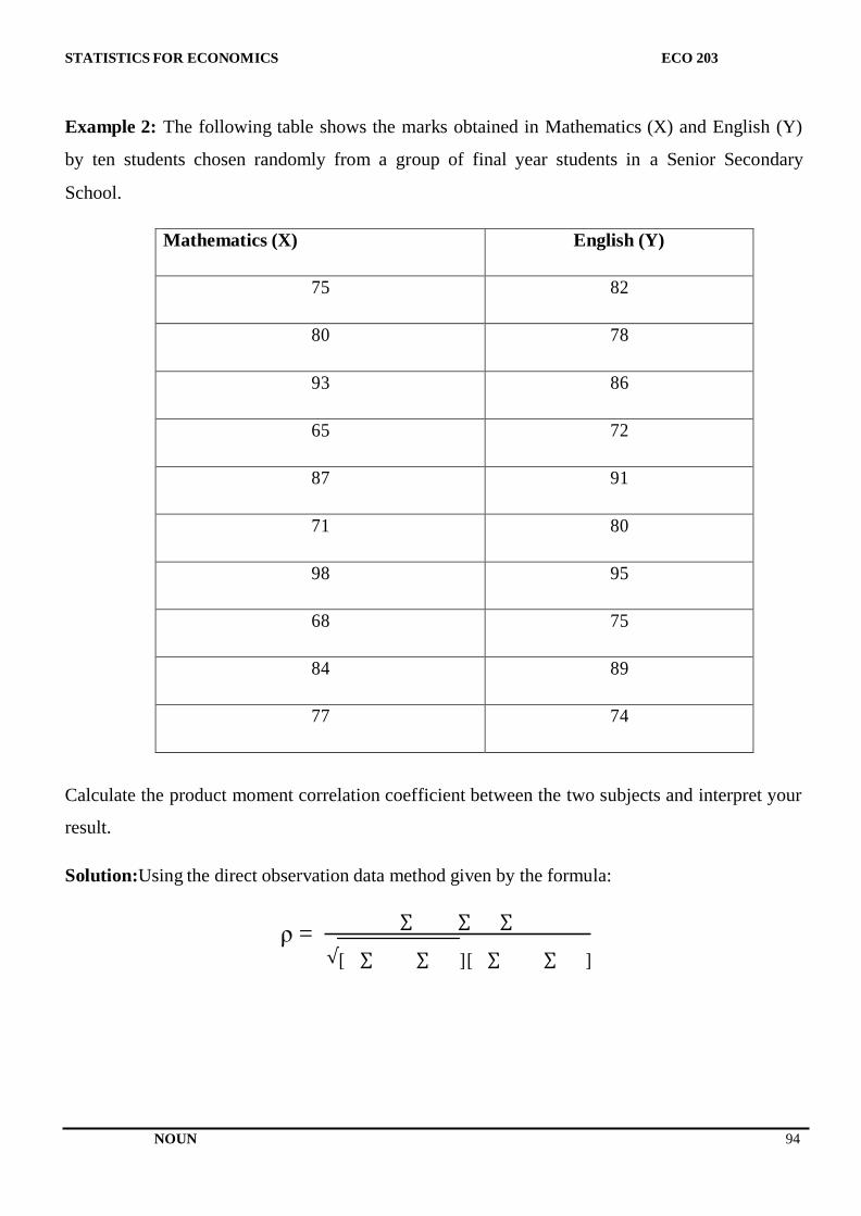
STATISTICS FOR ECONOMICS ECO 203
NOUN 94
Example 2: The following table shows the marks obtained in Mathematics (X) and English (Y)
by ten students chosen randomly from a group of final year students in a Senior Secondary
School.
Mathematics (X) English (Y)
75 82
80 78
93 86
65 72
87 91
71 80
98 95
68 75
84 89
77 74
Calculate the product moment correlation coefficient between the two subjects and interpret your
result.
Solution:Using the direct observation data method given by the formula:
∑ ∑ ∑ ρ =
√[ ∑ ∑ ][ ∑ ∑ ]
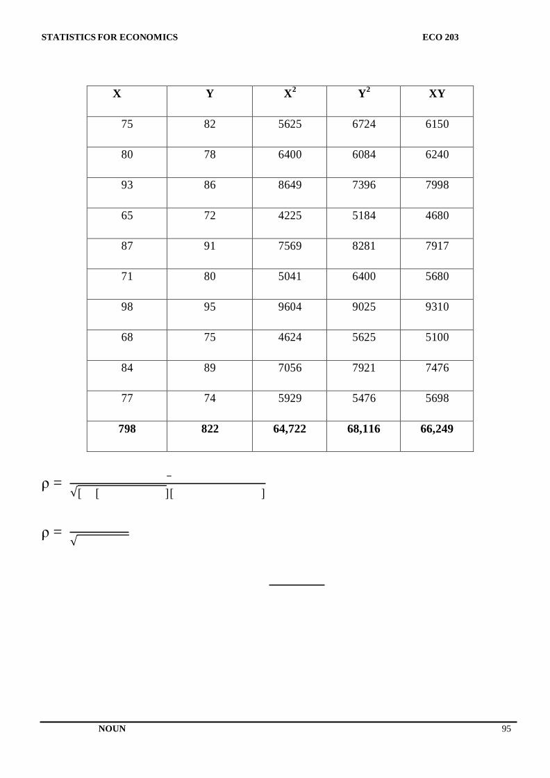
STATISTICS FOR ECONOMICS ECO 203
NOUN 95
X Y X2 Y
2 XY
75 82 5625 6724 6150
80 78 6400 6084 6240
93 86 8649 7396 7998
65 72 4225 5184 4680
87 91 7569 8281 7917
71 80 5041 6400 5680
98 95 9604 9025 9310
68 75 4624 5625 5100
84 89 7056 7921 7476
77 74 5929 5476 5698
798 822 64,722 68,116 66,249
ρ = –
√[ [ ][ ]
ρ = √
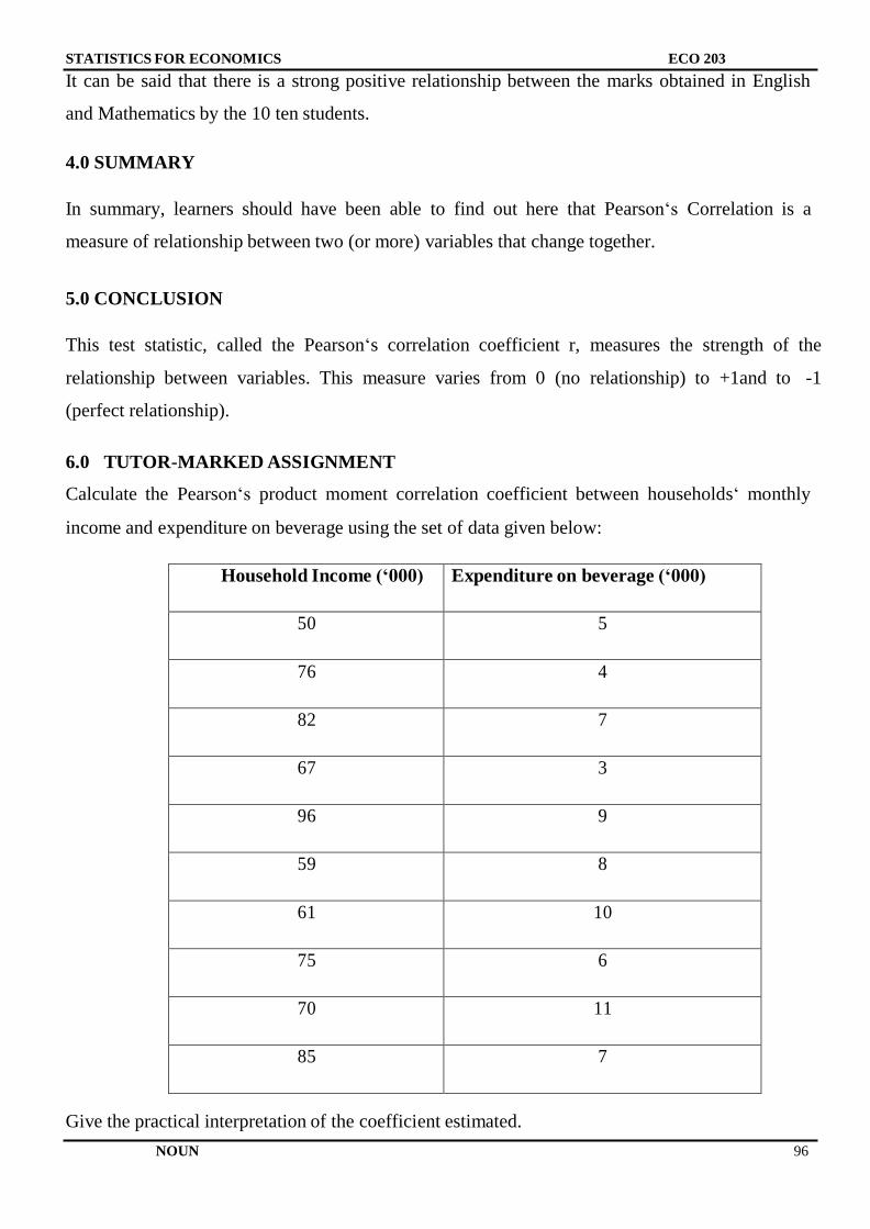
STATISTICS FOR ECONOMICS ECO 203
NOUN 96
It can be said that there is a strong positive relationship between the marks obtained in English
and Mathematics by the 10 ten students.
4.0 SUMMARY
In summary, learners should have been able to find out here that Pearson‘s Correlation is a
measure of relationship between two (or more) variables that change together.
5.0 CONCLUSION
This test statistic, called the Pearson‘s correlation coefficient r, measures the strength of the
relationship between variables. This measure varies from 0 (no relationship) to +1and to -1
(perfect relationship).
6.0 TUTOR-MARKED ASSIGNMENT
Calculate the Pearson‘s product moment correlation coefficient between households‘ monthly
income and expenditure on beverage using the set of data given below:
Household Income (‘000) Expenditure on beverage (‘000)
50 5
76 4
82 7
67 3
96 9
59 8
61 10
75 6
70 11
85 7
Give the practical interpretation of the coefficient estimated.

STATISTICS FOR ECONOMICS ECO 203
NOUN 97
7.0 REFERENCES/FURTHER READING
Spiegel M. R. and Stephens L. J. (2008).Statistics. (4th ed.). New York: McGraw Hill Press.
Gupta S.C. (2011). Fundamentals of Statistics. (6th Rev. and Enlarged ed.). Mumbai, India:
Himalayan Publishing House.
Swift L. (1997). Mathematics and Statistics for Business, Management and Finance. London:
Macmillan.
STATISTICS FOR ECONOMICS ECO 203
NOUN 98
UNIT 2: SPEARMAN’S RANK CORRELATION METHOD
CONTENTS
1.0 Objectives
2.0 Introduction
3.0 Main Content
4.0 Summary
5.0 Conclusion
6.0 Tutor-Marked Assignment
7.0 References/Further Reading
1.0 OBJECTIVES
Since Spearman‘s rho/Rank Correlation Coefficient is a nonparametric measure of correlation
coefficient, the aim here is to explain how Spearman‘s rho is used when your data does not
conformto the assumptions of a parametric test.
2.0 INTRODUCTION
In certain instances, we come across statistical series in the variables under consideration cannot
be measured quantitatively but can only be arranged in serial order. This is always the situation
when we are dealing with qualitative attributes such as intelligence, preference, honesty, morality
etc. In such case, Karl Pearson‘s coefficient of correlation cannot be used. A British Psychologist
Charles Edward Spearman developed a formula in 1904 which can be used to obtain the
correlation coefficient between the ranks of n individuals in the two variables or attributes being
study.
For example, assuming we are interested in determining the correlation between fluency in
English Language (A) and Beauty (B) among a group young ladies numbering n. These are
variables which cannot be measured but we can arrange the group of n individuals in order of
merit (ranks) with respect to their proficiency in the two attributes. Let the random variables X
STATISTICS FOR ECONOMICS ECO 203
NOUN 99
and Y denote the rank of the individuals in the characteristics A and B respectively. Also, if it is
assumed that there is no tie, i.e no two individuals get the same rank in a characteristic, then, X
and Y assume numerical values ranging from 1 to n.
Spearman‘s Rank Correlation Coefficient, usually denoted by ρ (Rho) is given by the formula:
∑
Where d is the difference between the pair of ranks of the same individual in the two
characteristics and n is the number of pairs.
3.0 MAIN CONTENT
Spearman's correlation coefficient measures correlation when the data is non-parametric, when
either x or y is not a continuous and normally distributed measurement.
Example 1:Fifteen members of staff of the administrative unit of an organization were studied to
determine the correlation between their punctuality at work (X) and the compliance of their
dresses with organizational dress code (Y) and the following ranks as given in the table below
were observed:
Rank in (X) 1 2 3 4 5 6 7 8 9 10 11 12 13 14 15
Rank in (Y) 10 7 2 6 4 8 3 1 11 15 9 5 14 12 13
Calculate the Spearman‘s rank correlation coefficient between the two characteristics.
Solution:
Spearman‘s Rank Correlation Coefficient is given by the formula:
∑
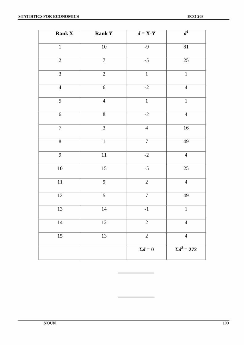
STATISTICS FOR ECONOMICS ECO 203
NOUN 100
Rank X Rank Y d = X-Y d2
1 10 -9 81
2 7 -5 25
3 2 1 1
4 6 -2 4
5 4 1 1
6 8 -2 4
7 3 4 16
8 1 7 49
9 11 -2 4
10 15 -5 25
11 9 2 4
12 5 7 49
13 14 -1 1
14 12 2 4
15 13 2 4
Σd = 0 Σd2
= 272
STATISTICS FOR ECONOMICS ECO 203
NOUN 101
, ,
Some challenging cases may arise when using Spearman’s rank correlation method: These
include:
Case I: When ranks are not given: The Edward Spearman‘s rank correlation formula can be
used even when dealing with variables which are measured quantitatively, i.e. when the actual
data but not the ranks relating to two variables are given. In such case, we shall have to convert
the data into ranks. The highest (or smallest) observation is given rank 1. The next highest (or
next lowest) observation is given rank 2and so on. It does not matter in which way (ascending or
descending) the ranks are assigned. However, the same approach should be followed for all the
variables under consideration.
Case II: Repeated ranks: In case of attributes, if there is a tie, i.e. if any two or more individuals
are placed together in any classification with respect to an attributes or if in any case of variable
data there are more than one items with the same value in either or both the series, then the
Spearman‘s formula for calculating the rank correlation coefficient breaks down, since in this case
the variable X (the rank of individuals in the first characteristic series) and Y (the rank of
individuals in the second characteristics series) do not take the values from 1 to n and
consequently as assumed in the derivation of the formula. In such instance, common
ranks are assigned to the repeated items. The common rank assigned is the arithmetic mean of the
ranks which these items would have got if they were different from each other and the next item
will get the rank next to the rank used in computing the common ran. For example, suppose an
item is repeated at rank 6, then the common rank to be assigned to each of the two items is
(6+7)/2 i.e. 6.5which is the average of 6 and 7, the ranks which the two observations would have
assumed if they were different. Therefore, the next item will be assigned the rank 8. Meanwhile, if
an item is repeated thrice at 9 for instance, then the common rank to be assigned to each of the
three will be (9+10+11)/3 i.e. 10which is the arithmetic mean of the three ranks. The next rank to
be assigned will be 12.
Example 2: Calculate the Spearman‘s rank correlation coefficient between advert expenditure and
sales revenue recorded by some randomly selected companies in an industrial estate as given
below:
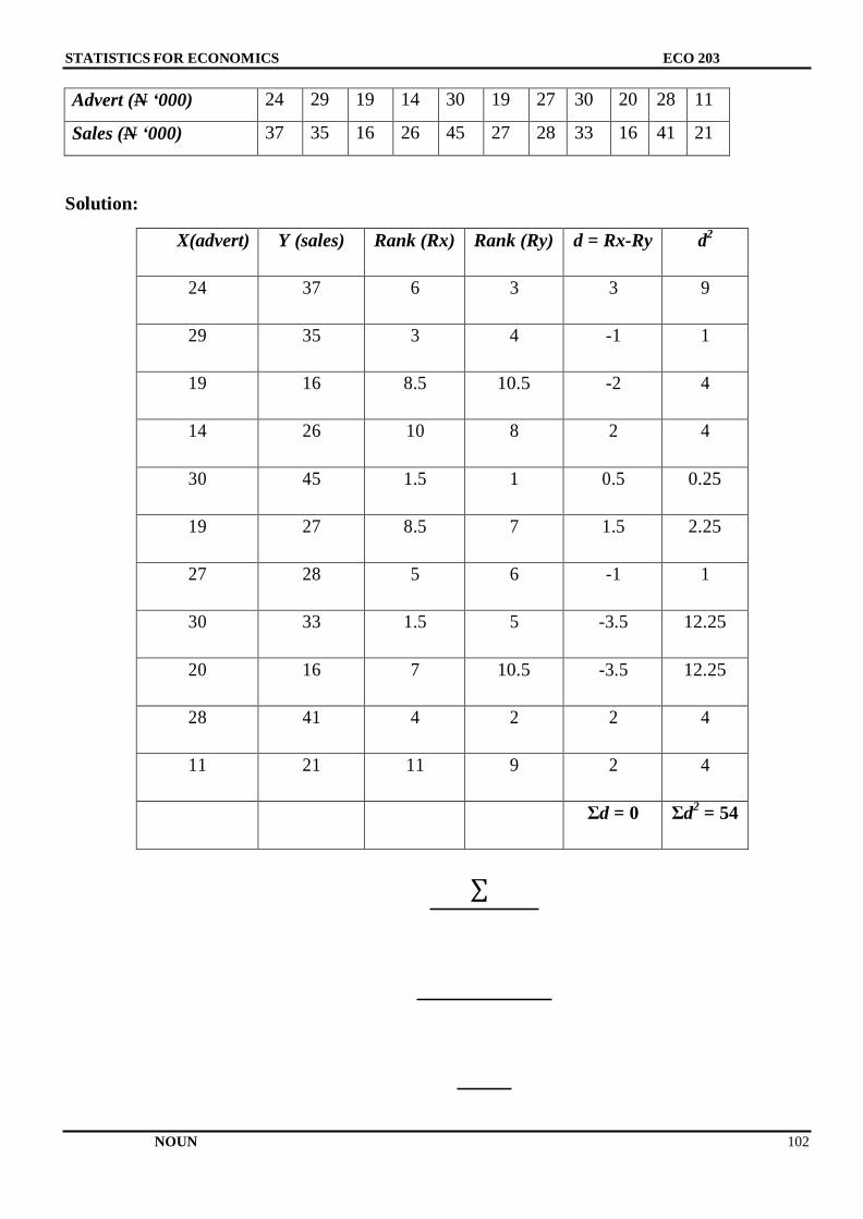
STATISTICS FOR ECONOMICS ECO 203
NOUN 102
Advert (N ‘000) 24 29 19 14 30 19 27 30 20 28 11
Sales (N ‘000) 37 35 16 26 45 27 28 33 16 41 21
Solution:
X(advert) Y (sales) Rank (Rx) Rank (Ry) d = Rx-Ry d2
24 37 6 3 3 9
29 35 3 4 -1 1
19 16 8.5 10.5 -2 4
14 26 10 8 2 4
30 45 1.5 1 0.5 0.25
19 27 8.5 7 1.5 2.25
27 28 5 6 -1 1
30 33 1.5 5 -3.5 12.25
20 16 7 10.5 -3.5 12.25
28 41 4 2 2 4
11 21 11 9 2 4
Σd = 0 Σd2
= 54
∑
STATISTICS FOR ECONOMICS ECO 203
NOUN 103
4.0SUMMARY
This unit by now has been able to help learners to calculate and interpret the simple correlation
between two variables and to determine whether the correlation is significant.
5.0CONCLUSION
Spearman's correlation coefficient approximates Pearson's correlation when the sample size is
large. Significant tests become problematic when sample size is less than 20, and specific tables of
probability will need to be consulted.
6.0 TUTOR-MARKED ASSIGNMENT
The following are the marks obtained by a group of students in two papers. Calculate the rank
coefficient of correlation.
Economics: 78 36 98 25 75 82 92 62 65 39
Statistics: 84 51 91 69 68 62 86 58 35 49
7.0 REFERENCES/FURTHER READING
Armitage P. (1980) Statistical Methods in Medical Research.Oxford:Blackwell Scientific
Publications, ISBN 0-632-05430-1 p. 147-166.
Siegel S. and Castellan Jr. N. J. (1988).Nonparametric Statistics for the Behavioral Sciences,(2nd.
ed.).Boston Massachusetts:McGraw Hill, Inc. ISBN 0-07-057357-3 p235-244.
STATISTICS FOR ECONOMICS ECO 203
NOUN 104
UNIT 4: LEAST SQUARE REGRESSION ANALYSIS
CONTENTS
1.0 Objectives
2.0 Introduction
3.0 Main Content
4.0 Summary
5.0 Conclusion
6.0 Tutor-Marked Assignment
7.0 References/Further Reading
1.0 OBJECTIVE
The objective of this unit is to expose learners to understanding and importance of the basic idea
of regression/correlation analysis being to predict the behaviour of one variable (the predict and)
based on fluctuations in one or more related variables (thepredictors). That, It is possible to
estimate the behaviour of the predict and using multiple predictors (multiple regression), and it is
also possible to predict the behavior of the predict and based on nonlinear relationships with the
predictors.
2.0 INTRODUCTION
If two variables are significantly correlated, and if there is some theoretical basis for doing so, it is
possible to predict values of one variable from the other. This observation leads to a very
important concept known as ‗Regression Analysis‘.
The literal or dictionary meaning of the word ―regression‖ is ―stepping back or returning to the
average value‖. The term was first used by the British Biometrician Sir Francis Galton in late 19th
century in connection with some studies he conducted on estimating the extent to which the
stature of the sons of tall parents reverts or regresses back to the mean stature of the population.
STATISTICS FOR ECONOMICS ECO 203
NOUN 105
He studied the relationship between the heights of about one thousand fathers and sons and
published the results in a paper ―Regression towards Mediocrity in Hereditary Stature‖.
Regression analysis, in general sense, means the estimation or prediction of the unknown value of
one variable from the known value of the other variable. It is one of the most important statistical
tools which are extensively used in almost all sciences – Natural, Social and Physical. It is
specially used in business and economics to study the relationship betweentwo or more variables
that are related causally and for the estimation of demand and supply graphs, cost functions,
production and consumption functions and so on.
Prediction or estimation is one of the major problems in almost all the spheres of human activity.
The estimation or prediction of future production, consumption, prices, investments, sales, profits,
income etc. are of very great importance to business professionals. Similarly, population estimates
and population projections, GNP, Revenue and Expenditure etc. areindispensable for economists
and efficient planning of an economy.
Regression analysis was explained by M. M. Blair as follows: ―Regression analysis is a
mathematical measure of the average relationship between two or more variables in terms of the
original units of the data.‖
Simple Regression: This a type of regression in which more than two variables are studied. This
is always the case in our day-to-day life because more often than not, a particular phenomenon is
affected by multiplicity of factors. For example, demand for a particular product is not only
determined by its market price but also by prices of substitutes, income of buyers, population and
taste and fashion among others.In regression analysis there are two types of variables and these
are:
Dependent Variable: This is the variable whose value is influenced or is to be predicted. For
example, elementary economic theory states that ―the higher the price the lower the quantity
demanded‖ In this, it is clear that quantity demanded is influenced by price of the commodity.
Therefore, quantity demanded of the commodity is described as the ―Dependent variable‖
Independent Variable: This is the variable which influences the value of the dependent variable
or which is used for prediction. In our example involving the law of demand, price of the
commodity determines or influences the quantity demanded. Therefore, price is described as the
―independent variable‖.
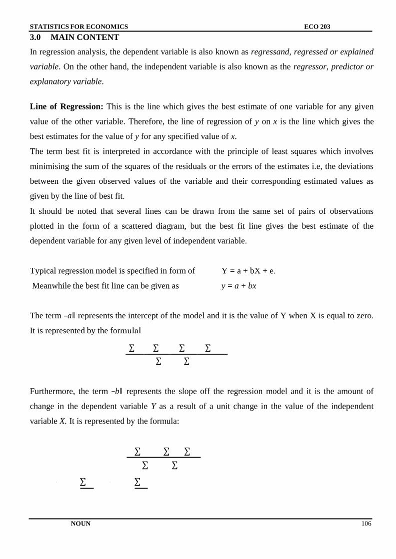
STATISTICS FOR ECONOMICS ECO 203
NOUN 106
3.0 MAIN CONTENT
In regression analysis, the dependent variable is also known as regressand, regressed or explained
variable. On the other hand, the independent variable is also known as the regressor, predictor or
explanatory variable.
Line of Regression: This is the line which gives the best estimate of one variable for any given
value of the other variable. Therefore, the line of regression of y on x is the line which gives the
best estimates for the value of y for any specified value of x.
The term best fit is interpreted in accordance with the principle of least squares which involves
minimising the sum of the squares of the residuals or the errors of the estimates i.e, the deviations
between the given observed values of the variable and their corresponding estimated values as
given by the line of best fit.
It should be noted that several lines can be drawn from the same set of pairs of observations
plotted in the form of a scattered diagram, but the best fit line gives the best estimate of the
dependent variable for any given level of independent variable.
Typical regression model is specified in form of Y = a + bX + e.
Meanwhile the best fit line can be given as y = a + bx
The term ―a‖ represents the intercept of the model and it is the value of Y when X is equal to zero.
It is represented by the formula‖
∑ ∑ ∑ ∑
∑ ∑
Furthermore, the term ―b‖ represents the slope off the regression model and it is the amount of
change in the dependent variable Y as a result of a unit change in the value of the independent
variable X. It is represented by the formula:
∑ ∑ ∑ ∑ ∑
∑ ∑
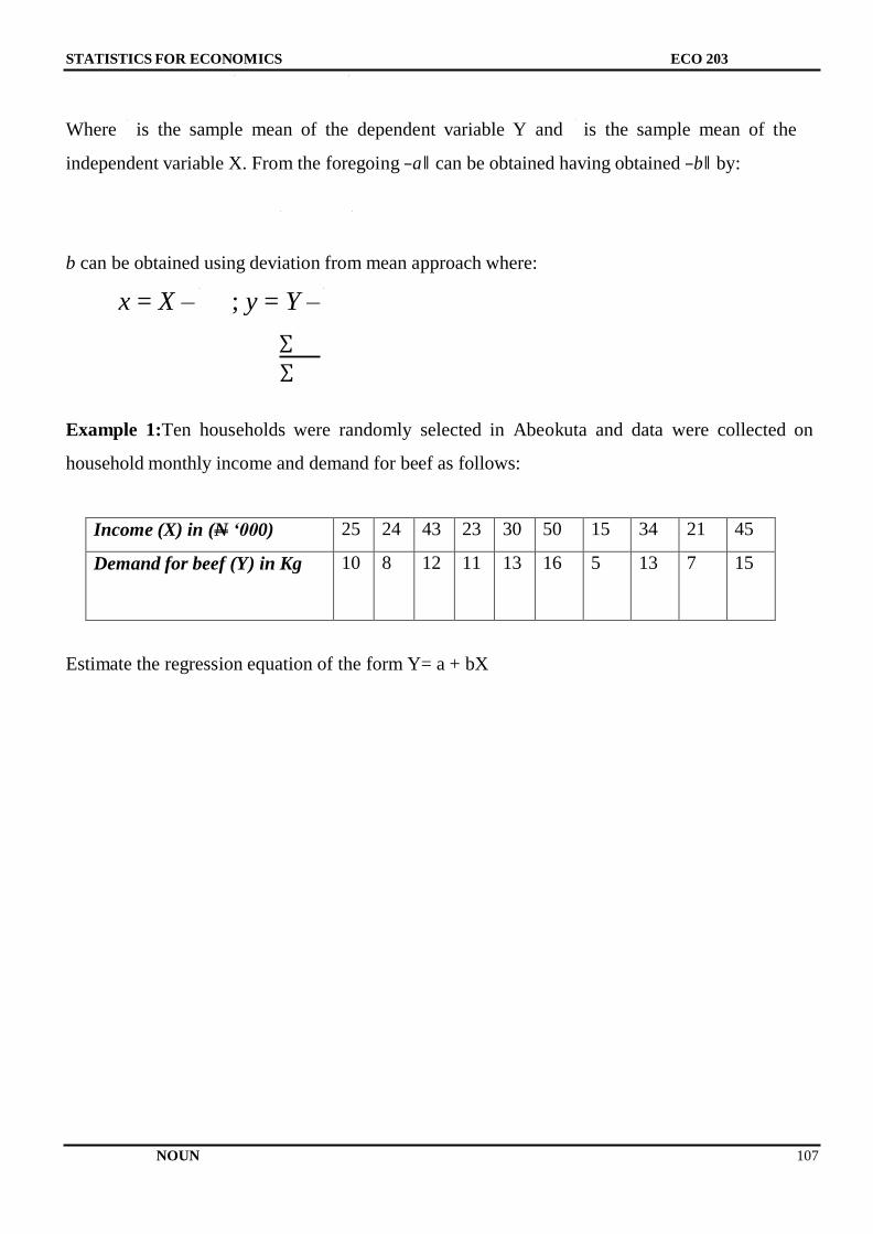
STATISTICS FOR ECONOMICS ECO 203
NOUN 107
Where is the sample mean of the dependent variable Y and is the sample mean of the
independent variable X. From the foregoing ―a‖ can be obtained having obtained ―b‖ by:
b can be obtained using deviation from mean approach where:
x = X – ; y = Y –
∑
∑
Example 1:Ten households were randomly selected in Abeokuta and data were collected on
household monthly income and demand for beef as follows:
Income (X) in (N ‘000) 25 24 43 23 30 50 15 34 21 45
Demand for beef (Y) in Kg 10 8 12 11 13 16 5 13 7 15
Estimate the regression equation of the form Y= a + bX
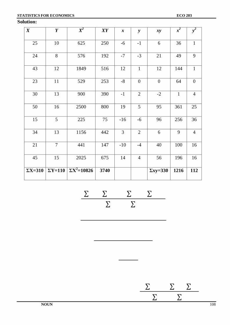
STATISTICS FOR ECONOMICS ECO 203
NOUN 108
Solution:
X Y X2 XY x y xy x
2 y
2
25 10 625 250 -6 -1 6 36 1
24 8 576 192 -7 -3 21 49 9
43 12 1849 516 12 1 12 144 1
23 11 529 253 -8 0 0 64 0
30 13 900 390 -1 2 -2 1 4
50 16 2500 800 19 5 95 361 25
15 5 225 75 -16 -6 96 256 36
34 13 1156 442 3 2 6 9 4
21 7 441 147 -10 -4 40 100 16
45 15 2025 675 14 4 56 196 16
ΣX=310 ΣY=110 ΣX2=10826 3740 Σxy=330 1216 112
∑ ∑ ∑ ∑
∑ ∑
∑ ∑ ∑
∑ ∑
STATISTICS FOR ECONOMICS ECO 203
NOUN 109
Alternatively, having obtained estimate value for the slope parameter b, the intercept term a can
be obtained using the formula:
In the above problem ∑ ∑
–
4.0 SUMMARY
With reference to the explanations and illustrations demonstrated above, learners can now apply
least square method to study the nature of the relation between two variables.
5.0 CONCLUSION A line of best fit can be roughly determined using an eyeball method by drawing a straight line
on a scatter plot so that the number of points above the line and below the line is about equal
(and the line passes through as many points as possible). A more accurate way of finding the
line of best fit is the least square method.
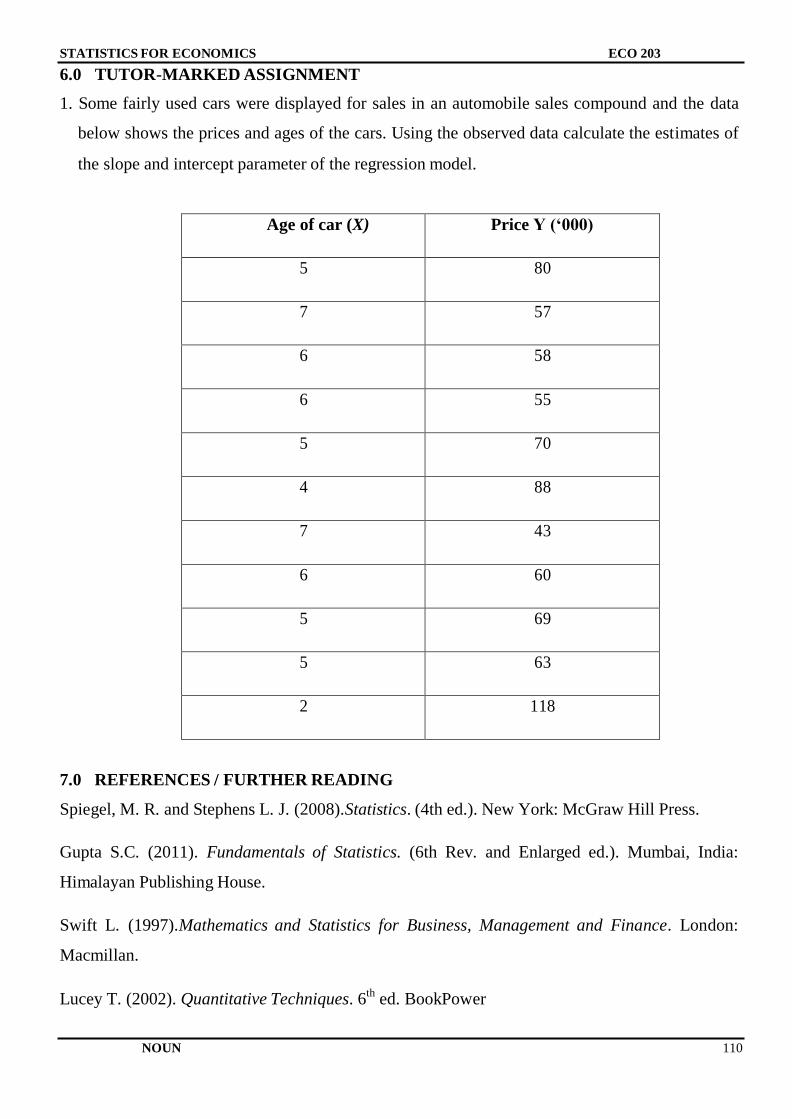
STATISTICS FOR ECONOMICS ECO 203
NOUN 110
6.0 TUTOR-MARKED ASSIGNMENT
1. Some fairly used cars were displayed for sales in an automobile sales compound and the data
below shows the prices and ages of the cars. Using the observed data calculate the estimates of
the slope and intercept parameter of the regression model.
Age of car (X) Price Y (‘000)
5 80
7 57
6 58
6 55
5 70
4 88
7 43
6 60
5 69
5 63
2 118
7.0 REFERENCES / FURTHER READING
Spiegel, M. R. and Stephens L. J. (2008).Statistics. (4th ed.). New York: McGraw Hill Press.
Gupta S.C. (2011). Fundamentals of Statistics. (6th Rev. and Enlarged ed.). Mumbai, India:
Himalayan Publishing House.
Swift L. (1997).Mathematics and Statistics for Business, Management and Finance. London:
Macmillan.
Lucey T. (2002). Quantitative Techniques. 6th
ed. BookPower
STATISTICS FOR ECONOMICS ECO 203
NOUN 111
UNIT 5: FORECASTING IN REGRESSION
CONTENTS
1.0 Objectives
2.0 Introduction
3.0 Main Content
4.0 Summary
5.0 Conclusion
6.0 Tutor-Marked Assignment
7.0 References/Further Reading
1.0 OBJECTIVE
Our aim in this unit is to usea given value of independent variables to predict the value of
dependent variable.
2.0 INTRODUCTION
In general, we are interested in point forecasts, which predict a single number in each forecast
period. Needless to say, the information provided by the forecasts can be very useful. For
instance, it can help not only in policy and decision making, but also in validating the model from
which the forecasts are made. In the forecasting process, we are usually given the values of the
independent variables and our goal is to predict the value of the dependent variable. This raises
the question of whether the values of the independent variables are known with certainty. If so,
then we are making an unconditional forecast. Otherwise, we are making a conditional forecast.
To see the difference between the two, consider the following settings:
1. Suppose that we use the following linear regression model to describe the relationship
between the demand for beef and household income Y = a + bX + u as used in the previous
unit. Once we obtain estimators of the regression parameters a; b, we can use the resulting
regression line to make forecasts. Specifically, the forecasted household demand for beef
will be given by . Sometimes, the value X which is the household income may
STATISTICS FOR ECONOMICS ECO 203
NOUN 112
depend on some unpredictable factors that are not known with certainty at the time of
forecast. Thus, our forecast for Y will be conditional on our forecast for X.
2. Suppose that we use the linear regression model to describe the relationship betweenthe
monthly auto sales stand the production capacity Ct:
St= a + bCt-2 + ϵt:
In other words, sales in the t-th month depends linearly on the production capacity of the
(t-2)nd month. If we are currently at the T-th month and we want to forecast the auto sales in the
(T +1)-st month, then we need the production capacity of the (T-1)st month, which can be
determined with certainty. Thus, in this case, the forecast will be unconditional.
3.0 MAIN CONTENT
Model Evaluation
The various ways to evaluate the reliability of a linear regression model include:
_ the t and F, which test the explanatory power of the independent variables;
_ the R2
which measures the goodness of fit; and
_ the forecast confidence interval.
It should be noted that these are quite different measures of model reliability, and they need not
subsume each other. For instance, a regression model can have significant t{statistics and a high
R2
value, and yet it still forecasts poorly. This could happen if there is a structural change in the
system during the forecasting period, which occurs after the estimation period (i.e., the period
during which we collect data and estimate the coefficients of the regression model). On the other
hand, one may be able to obtain good forecasts from regression models that have insignificant
regression coefficients or relatively low R2
values. This could happen when there is very little
variation in the dependent variable, so that although it is not well explained by the regression
model, it can still be forecast easily
Example: Let us use our example on the household demand for beef in Abeokuta which was
states thus: Ten households were randomly selected in Abeokuta and data were collected on
household monthly income and demand for beef as follows:
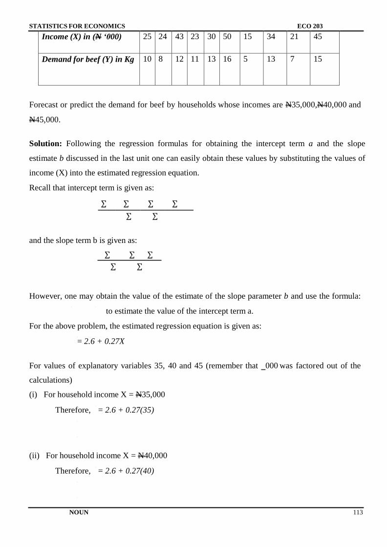
STATISTICS FOR ECONOMICS ECO 203
NOUN 113
Income (X) in (N ‘000) 25 24 43 23 30 50 15 34 21 45
Demand for beef (Y) in Kg 10 8 12 11 13 16 5 13 7 15
Forecast or predict the demand for beef by households whose incomes are N35,000,N40,000 and
N45,000.
Solution: Following the regression formulas for obtaining the intercept term a and the slope
estimate b discussed in the last unit one can easily obtain these values by substituting the values of
income (X) into the estimated regression equation.
Recall that intercept term is given as:
∑ ∑ ∑ ∑
∑ ∑
and the slope term b is given as:
∑ ∑ ∑
∑ ∑
However, one may obtain the value of the estimate of the slope parameter b and use the formula:
to estimate the value of the intercept term a.
For the above problem, the estimated regression equation is given as:
= 2.6 + 0.27X
For values of explanatory variables 35, 40 and 45 (remember that ‗000 was factored out of the
calculations)
(i) For household income X = N35,000
Therefore, = 2.6 + 0.27(35)
(ii) For household income X = N40,000
Therefore, = 2.6 + 0.27(40)
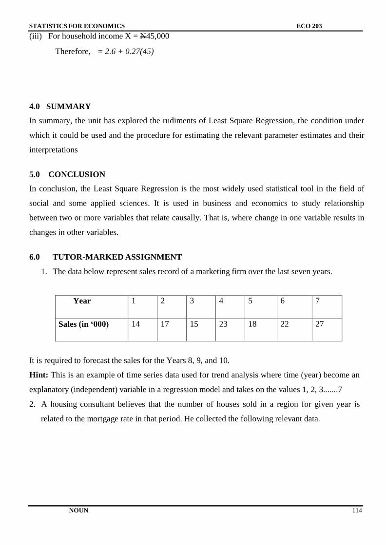
STATISTICS FOR ECONOMICS ECO 203
NOUN 114
(iii) For household income X = N45,000
Therefore, = 2.6 + 0.27(45)
4.0 SUMMARY
In summary, the unit has explored the rudiments of Least Square Regression, the condition under
which it could be used and the procedure for estimating the relevant parameter estimates and their
interpretations
5.0 CONCLUSION
In conclusion, the Least Square Regression is the most widely used statistical tool in the field of
social and some applied sciences. It is used in business and economics to study relationship
between two or more variables that relate causally. That is, where change in one variable results in
changes in other variables.
6.0 TUTOR-MARKED ASSIGNMENT
1. The data below represent sales record of a marketing firm over the last seven years.
Year 1 2 3 4 5 6 7
Sales (in ‘000) 14 17 15 23 18 22 27
It is required to forecast the sales for the Years 8, 9, and 10.
Hint: This is an example of time series data used for trend analysis where time (year) become an
explanatory (independent) variable in a regression model and takes on the values 1, 2, 3.......7
2. A housing consultant believes that the number of houses sold in a region for given year is
related to the mortgage rate in that period. He collected the following relevant data.
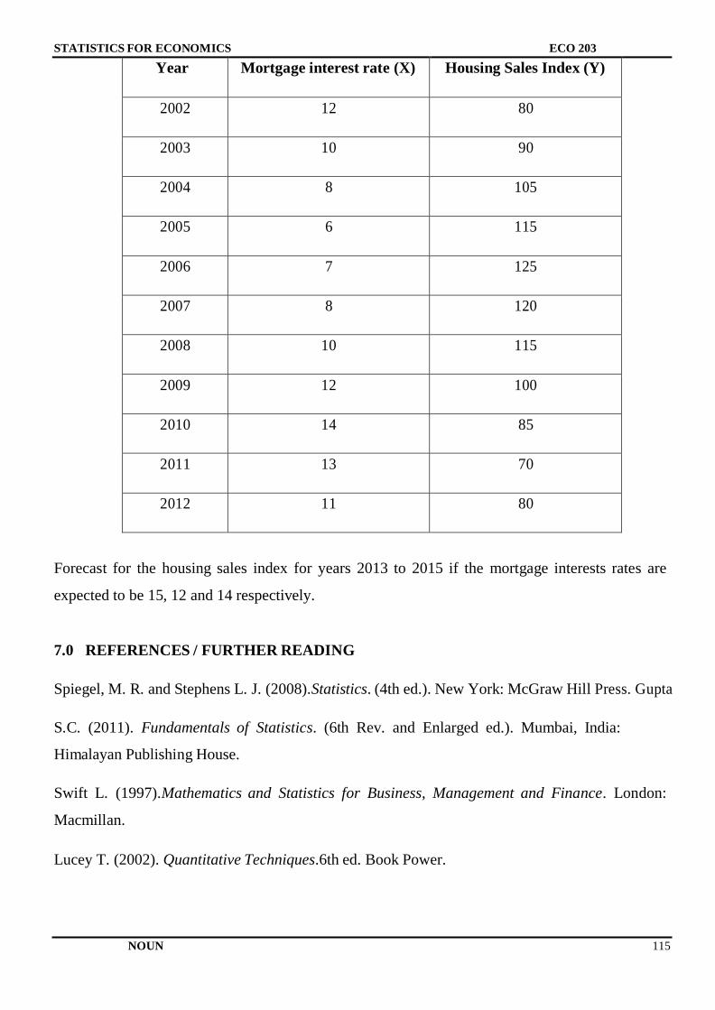
STATISTICS FOR ECONOMICS ECO 203
NOUN 115
Year Mortgage interest rate (X) Housing Sales Index (Y)
2002 12 80
2003 10 90
2004 8 105
2005 6 115
2006 7 125
2007 8 120
2008 10 115
2009 12 100
2010 14 85
2011 13 70
2012 11 80
Forecast for the housing sales index for years 2013 to 2015 if the mortgage interests rates are
expected to be 15, 12 and 14 respectively.
7.0 REFERENCES / FURTHER READING
Spiegel, M. R. and Stephens L. J. (2008).Statistics. (4th ed.). New York: McGraw Hill Press. Gupta
S.C. (2011). Fundamentals of Statistics. (6th Rev. and Enlarged ed.). Mumbai, India:
Himalayan Publishing House.
Swift L. (1997).Mathematics and Statistics for Business, Management and Finance. London:
Macmillan.
Lucey T. (2002). Quantitative Techniques.6th ed. Book Power.
STATISTICS FOR ECONOMICS ECO 203
NOUN 116
MODULE 4 INTRODUCTION TO THE CENTRAL LIMIT THEORY (CLT)
Central limit theorem: it states that given a sufficiently large sample size from a population with a
finite level of variance, the mean of all samples from the same population will be approximately
equal to the mean of the population. Furthermore, all the samples will follow an approximate
normal distribution pattern, with a variance being approximately equal to the variance of the
population divided by the sample size. This Module is divided into five units. These are:
Unit 1: Central Limit Theorems for Independent Sequences
Unit 2: Central Limit Theorems for dependent Processes
Unit 3: Relation to the law of large numbers
Unit 4: Extensions to the theorem of CLT and Beyond the classical framework
UNIT 1: THE CENTRAL LIMIT THEOREM FOR INDEPENDENT SEQUENCECONTENTS
1.0 Objectives
2.0 Introduction
3.0 Main Content
3.1 CLT Rules
3.2 Classical CLTs
4.0 Summary
5.0 Conclusion
6.0 Tutor-Marked Assignment
7.0 References/Further Reading
STATISTICS FOR ECONOMICS ECO 203
NOUN 117
1.0 OBJECTIVE
The main aim here is to expose learners to the importance ofCentral Limit Theorem (CLT) for
independent sequence in understanding inferential statistics and hypothesis testing.
2.0 INTRODUCTION
If a random sample of N cases is drawn from a population with a mean µ and standard deviation s,
then the sampling distribution of the mean has:
1. a mean equal to the population mean µx
2. a standard deviation (standard error) equal to the standard deviation divided by the square
root of the sample size N: √
3. the shape of the sampling distribution of the mean approaches normal as N increases.
3.0 MAIN CONTENT
3.1 CLT Rules
Let‘s denote the mean of the observations in a random sample of size n from a population having
a mean µ and standard deviation σ. Denote the mean of the Y distribution by µYand the standard
deviation of the Y distribution by σ ӯ.
Then the following rules hold:
Rule 1.µӯ = µ
Rule 2. This rule is approximately correct as long as no more than 5% of the population is √
included in the sample.
Rule 3.When the population distribution is normal, the sampling distribution of Y is also normal
for any sample size n.
STATISTICS FOR ECONOMICS ECO 203
NOUN 118
Rule 4.When n is sufficiently large, the sampling distribution of Y is well approximated by a
normal curve, even when the population distribution is not itself normal.
Suppose that a sample of size n is selected from a population that has mean µ and standard
deviation ζ. Let X1;X2; _ _ _ Xn be the n observations that are independent and identically
distributed (i.i.d.). Define now the sample mean and the total of these n observations as
follows:
∑
∑
The central limit theorem states that the sample mean follows approximately the normal
distribution with mean µ and standard deviation √
, where µ and ζ are the mean and standard
deviation of the population from where the sample was selected. The sample size n has to be large
(usually n˃30) if the population from where the sample is taken is non-normal. If the population
follows the normal distribution then the sample size n can either be small or large. The sample
mean of a large random sample of random variables with mean μ and finite variance ζ2
has
approximately the normal distribution with mean μ and variance ζ2/n. This result helps to justify
the use of the normal distribution as a model for many random variables that can be thought of as
being made up of many independent parts. Another version of the central limit theorem is given
that applies to independent random variables that are not identically distributed.
To summarize: √
To transform into z we use:
√
STATISTICS FOR ECONOMICS ECO 203
NOUN 119
Let us suppose that Y1, Y2, Yn ,..., are independent and identically distributed with mean µand
finite variance σ2. We now prove these two theorems about the mean and variance of the sample
mean.
Theorem 1:
Proof:
* +
= [ ]
= [ ]
= [ ]
= [ ]
Theorem 2:
Proof:
* +
( ) [ ]
( ) [ ]
( ) [ ]
( ) [ ]
In probability theory central limit theorem states that given a certain conditions the mean of a
sufficiently large number of iterates.
STATISTICS FOR ECONOMICS ECO 203
NOUN 120
The CLT can tell us about the distribution of large sums of random variables even if the
distribution of the random variables is almost unknown. With this result we are able to
approximate how likely it is that the arithmetic mean deviates from its expected value.
Using the CLT we can verify hypotheses by making statistical decisions, because we are able to
determine the asymptotic distribution of certain test statistics.
⇒ √
i.e. a centred and normalized sum of independent and identically distributed (i.i.d.) random
variables is distributed standard normally as n goes to infinity.
Example: Let X be a random variable with µ = 10 and ζ = 4. A sample of size 100 is taken from
this population. Find the probability that the sample mean of these 100 observations is less than 9.
We write
( )
√
(from the standard normal probabilities table).
Similarly the central limit theorem states that sum T follows approximately the normal distribution, √ , where µ and ζ are the mean and standard deviation of the population
from where the sample was selected.
To transform T into z we use: √
3.2 Classical CLT
Let {X1, ..., Xn} be a random sample of size n — that is, a sequence of independent and identically
distributed random variables drawn from distributions of expected values given by µ and finite
variances given by ζ2. Suppose we are interested in the sample average
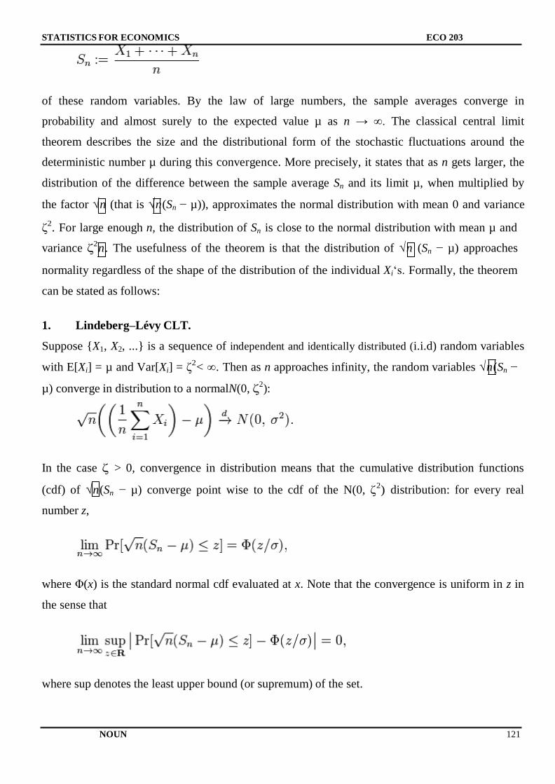
STATISTICS FOR ECONOMICS ECO 203
NOUN 121
of these random variables. By the law of large numbers, the sample averages converge in
probability and almost surely to the expected value µ as n → ∞. The classical central limit
theorem describes the size and the distributional form of the stochastic fluctuations around the
deterministic number µ during this convergence. More precisely, it states that as n gets larger, the
distribution of the difference between the sample average Sn and its limit µ, when multiplied by
the factor √n (that is √n(Sn − µ)), approximates the normal distribution with mean 0 and variance
ζ2. For large enough n, the distribution of Sn is close to the normal distribution with mean µ and
variance ζ2 n. The usefulness of the theorem is that the distribution of √n (Sn − µ) approaches
normality regardless of the shape of the distribution of the individual Xi‘s. Formally, the theorem
can be stated as follows:
1. Lindeberg–Lévy CLT.
Suppose {X1, X2, ...} is a sequence of independent and identically distributed (i.i.d) random variables
with E[Xi] = µ and Var[Xi] = ζ2< ∞. Then as n approaches infinity, the random variables √n(Sn −
µ) converge in distribution to a normalN(0, ζ2):
In the case ζ > 0, convergence in distribution means that the cumulative distribution functions
(cdf) of √n(Sn − µ) converge point wise to the cdf of the N(0, ζ2) distribution: for every real
number z,
where Φ(x) is the standard normal cdf evaluated at x. Note that the convergence is uniform in z in
the sense that
where sup denotes the least upper bound (or supremum) of the set.
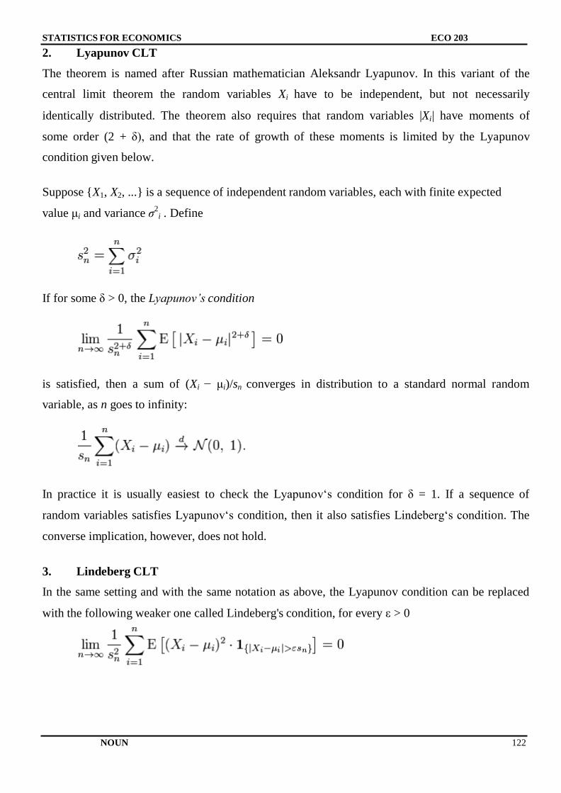
STATISTICS FOR ECONOMICS ECO 203
NOUN 122
2. Lyapunov CLT
The theorem is named after Russian mathematician Aleksandr Lyapunov. In this variant of the
central limit theorem the random variables Xi have to be independent, but not necessarily
identically distributed. The theorem also requires that random variables |Xi| have moments of
some order (2 + δ), and that the rate of growth of these moments is limited by the Lyapunov
condition given below.
Suppose {X1, X2, ...} is a sequence of independent random variables, each with finite expected
value μi and variance σ2
i . Define
If for some δ > 0, the Lyapunov’s condition
is satisfied, then a sum of (Xi − μi)/sn converges in distribution to a standard normal random
variable, as n goes to infinity:
In practice it is usually easiest to check the Lyapunov‘s condition for δ = 1. If a sequence of
random variables satisfies Lyapunov‘s condition, then it also satisfies Lindeberg‘s condition. The
converse implication, however, does not hold.
3. Lindeberg CLT
In the same setting and with the same notation as above, the Lyapunov condition can be replaced
with the following weaker one called Lindeberg's condition, for every ε > 0
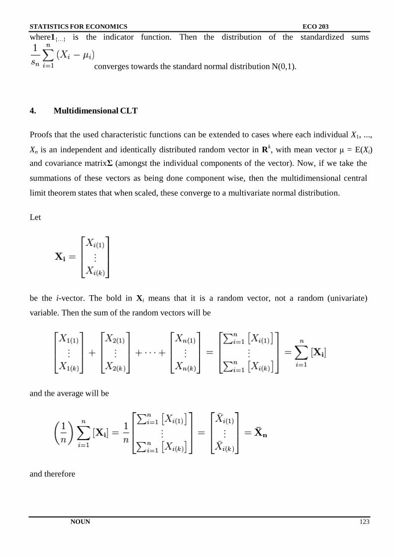
STATISTICS FOR ECONOMICS ECO 203
NOUN 123
where1{…} is the indicator function. Then the distribution of the standardized sums
converges towards the standard normal distribution N(0,1).
4. Multidimensional CLT
Proofs that the used characteristic functions can be extended to cases where each individual X1, ...,
Xn is an independent and identically distributed random vector in Rk, with mean vector μ = E(Xi)
and covariance matrixΣ (amongst the individual components of the vector). Now, if we take the
summations of these vectors as being done component wise, then the multidimensional central
limit theorem states that when scaled, these converge to a multivariate normal distribution.
Let
be the i-vector. The bold in Xi means that it is a random vector, not a random (univariate)
variable. Then the sum of the random vectors will be
and the average will be
and therefore
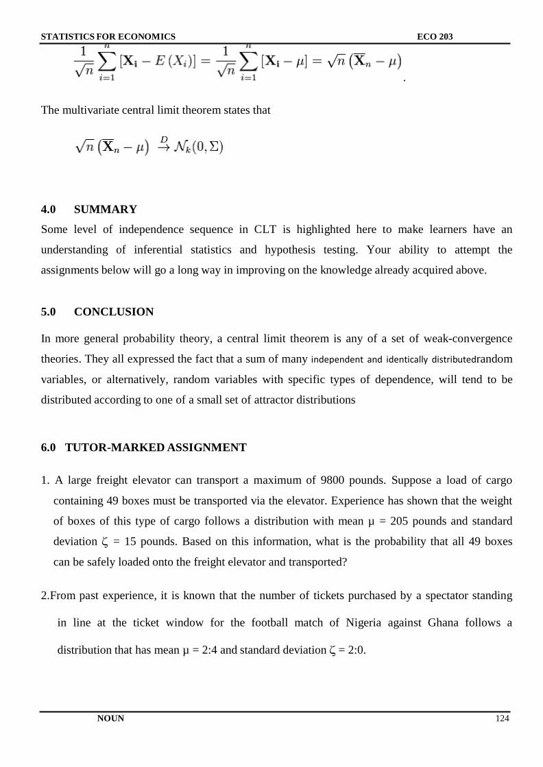
STATISTICS FOR ECONOMICS ECO 203
NOUN 124
.
The multivariate central limit theorem states that
4.0 SUMMARY
Some level of independence sequence in CLT is highlighted here to make learners have an
understanding of inferential statistics and hypothesis testing. Your ability to attempt the
assignments below will go a long way in improving on the knowledge already acquired above.
5.0 CONCLUSION
In more general probability theory, a central limit theorem is any of a set of weak-convergence
theories. They all expressed the fact that a sum of many independent and identically distributedrandom
variables, or alternatively, random variables with specific types of dependence, will tend to be
distributed according to one of a small set of attractor distributions
6.0 TUTOR-MARKED ASSIGNMENT
1. A large freight elevator can transport a maximum of 9800 pounds. Suppose a load of cargo
containing 49 boxes must be transported via the elevator. Experience has shown that the weight
of boxes of this type of cargo follows a distribution with mean µ = 205 pounds and standard
deviation ζ = 15 pounds. Based on this information, what is the probability that all 49 boxes
can be safely loaded onto the freight elevator and transported?
2.From past experience, it is known that the number of tickets purchased by a spectator standing
in line at the ticket window for the football match of Nigeria against Ghana follows a
distribution that has mean µ = 2:4 and standard deviation ζ = 2:0.
NOUN 125
STATISTICS FOR ECONOMICS ECO 203
Suppose that few hours before the start of one of these matches there are 100 eager spectators
standing in line to purchase tickets.
If only 250 tickets remain, what is the probability that all 100 students will be able to purchase
the tickets they desire?
7.0 REFERENCES/FURTHER READING
Billingsley, P. (1995), Probability and Measure (3rded.). John Wiley &Sons Publishers, ISBN0-
471-00710-2
Bradley, R. (2007), Introduction to Strong Mixing Conditions (1st ed.), Heber City, UT: Kendrick
Press, ISBN0-9740427-9-X
Bradley, R. (2005), Basic Properties of Strong Mixing Conditions. A Survey and Some Open
Questions, Probability Surveys2:107–144,
arXiv:math/0511078v1,doi:10.1214/154957805100000104, http://arxiv.org/pdf/math/0511078.pdf
Dinov, I., Christou, N. and Sanchez, J. (2008), Central Limit Theorem: New SOCR Applet and
Demonstration Activity, Journal of Statistics Education (ASA) 16 (2),
http://www.amstat.org/publications/jse/v16n2/dinov.html, website: www. Wikipedia.com
NOUN 126
STATISTICS FOR ECONOMICS ECO 203
UNIT 2 CENTRAL LIMIT THEOREM FOR DEPENDENT PROCESSES
CONTENTS
1.0 Objectives
2.0 Introduction
3.0 Main Content
3.1 CLT under weak dependence
3.2 Martingale difference CLT
6.0 Summary
7.0 Conclusion
8.0 .Tutor-Marked Assignment
7.0. References/Further Reading
1.0 OBJECTIVES
A main attraction of CLT sequences is to provide examples of processes that are weakly
dependent, but not mixing. This way of constructing stationary sequences is very natural.
2.0 INTRODUCTION
A useful generalization of a sequence of independent identically distributed random variables is a
mixing random process in discrete time; "mixing" means, roughly, that random variables
temporally far apart from one another are nearly independent. Several kinds of mixing are used in
ergodic theory and probability theory. Strong mixing (also called α-mixing) is defined by α(n) →
0 where α(n) is so-called strong mixing coefficient.
NOUN 127
STATISTICS FOR ECONOMICS ECO 203
3.0 MAIN CONTENT
A simplified formulation of the central limit theorem under strong mixing is provided for in the
following:
CLT under weak dependence
Martingale difference CLT
Theoremi. Suppose that X1, X2, … is stationary and α-mixing with αn = O(n−5
) and that E(Xn) = 0
and E(Xn12
) < ∞. Denote Sn = X1 + … + Xn, then the limit
exists, and if ζ ≠ 0 then √ converges in distribution to N(0, 1).
In fact, ∑
where the series converges absolutely.
The assumption ζ ≠ 0 cannot be omitted, since the asymptotic normality fails for Xn = Yn − Yn−1
where Yn are another stationary sequence.
There is a stronger version of the theorem: the assumption E(Xn12
) < ∞ is replaced with
E(|Xn|2 + δ
) < ∞, and the assumption αn = O(n−5
) is replaced with ∑
Existence of such δ > 0 ensures the conclusion.
Theoremii. Let a martingaleMn satisfy
∑ in probability as n tends to infinity,
NOUN 128
STATISTICS FOR ECONOMICS ECO 203
-for every ε >0 , ∑ | | √
Then √ converges in distribution to N(0,1) as n → ∞.
Proof of classical CLT
For a theorem of such fundamental importance to statistics and applied probability, the central
limit theorem has a remarkably simple proof using characteristic functions. It is similar to the
proof of a (weak) law of large numbers. For any random variable, Y, with zero mean and a unit
variance (var(Y) = 1), the characteristic function of Y is, by Taylor's theorem,
whereo (t2) is "little o notation" for some function of t that goes to zero more rapidly than t
2.
Letting Yi be (Xi − μ)/ζ, the standardized value of Xi, it is easy to see that the standardized mean of
the observations X1, X2, ..., Xn is
∑
√ √
By simple properties of characteristic functions, the characteristic function of Zn is
[ ( )] * ( )+ ⁄
√
But this limit is just the characteristic function of a standard normal distribution N(0, 1), and the
central limit theorem follows from the Lévy continuity theorem, which confirms that the
convergence of characteristic functions implies convergence in distribution.
4.0 SUMMARY
The central limit theorem applies in particular to sums of independent and identically distributed
discrete random variables. A sum of discrete random variables is still a discrete random variable,
so that we are confronted with a sequence of discrete random variables whose cumulative
probability distribution function converges towards a cumulative probability distribution function
NOUN 129
STATISTICS FOR ECONOMICS ECO 203
corresponding to a continuous variable (namely that of the normal distribution). This means that if
we build a histogram of the realisations of the sum of n independent identical discrete variables,
the curve that joins the centres of the upper faces of the rectangles forming the histogram
converges toward a Gaussian curve as n approaches infinity, this relation is known as de Moivre–
Laplace theorem. The binomial distribution article details such an application of the central limit
theorem in the simple case of a discrete variable taking only two possible values.
5.0 CONCLUSION
The central limit theorem gives only an asymptotic distribution. As an approximation for a finite
number of observations, it provides a reasonable approximation only when close to the peak of the
normal distribution; it requires a very large number of observations to stretch into the tails.
If the third central moment E((X1 − μ)3) exists and is finite, then the above convergence is uniform
and the speed of convergence is at least on the order of 1/n1/2
can be used not only to prove the
central limit theorem, but also to provide bounds on the rates of convergence for selected metrics.
The convergence to the normal distribution is monotonic, in the sense that the entropy of Zn
increases monotonically to that of the normal distribution.
6.0 TUTOR-MARKED ASSIGNMENT
1. Show how the Martingale converges towards normality as n tends towards infinity.
2. Explain how a series will converge towards the limit under the dependence process
7.0 REFERENCES/FURTHER READING
Artstein, S.; Ball, K.; Barthe, F. andNaor, A. (2004), "Solution of Shannon's Problem on the
Monotonicity of Entropy",Journal of the American Mathematical Society17 (4): 975–982,
doi:10.1090/S0894-0347-04-00459-X
Rosenthal, J. S. (2000) A first look at rigorous probability theory, World Scientific, ISBN 981-02-
4322-7.(Theorem 5.3.4, p. 47)
Website: www.wikipedia.com
NOUN 130
STATISTICS FOR ECONOMICS ECO 203
UNIT 3:THE LAW OF LARGE NUMBERS
CONTENTS
1.0 Objectives
2.0 Introduction
3.0 Main Content
4.0 Summary
5.0Conclusion
6.0 Tutor-Marked Assignment
7.0 References/Further Reading
1.0 OBJECTIVES
The aim here is to emphasize that the Law of Large Numbers (LLN) is important because it
"guarantees" stable long-term results for the averages of random events.
2.0 INTRODUCTION
It is a rule that assumes that as the number of samples increases, the average of the samples is
likely to reach the mean of the population. The law of large numbers says that the sample mean of
a random sample converges in probability to the mean μ of the individual random variables, if the
variance exists. This means that the sample mean will be close to μ if the size of the random
sample is sufficiently large.
Suppose that X1, . . . ,Xnform a random sample from a distribution for which the mean is μ and for
which the variance is finite. Let Xndenote the sample mean. Then
Proof:Let the variance of each Xi beσ2. It then follows from the Chebyshev inequality that for
every number ε >0,
| |
Hence,
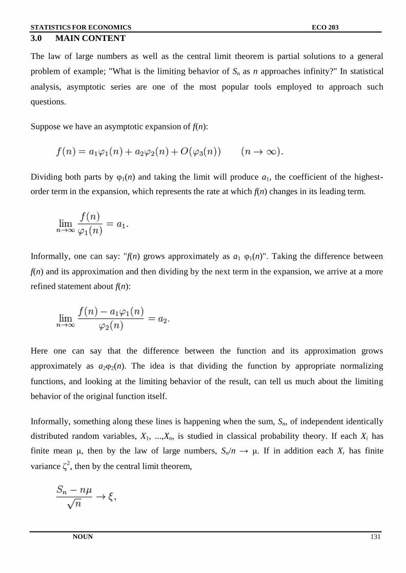
NOUN 131
STATISTICS FOR ECONOMICS ECO 203
3.0 MAIN CONTENT
The law of large numbers as well as the central limit theorem is partial solutions to a general
problem of example; "What is the limiting behavior of Sn as n approaches infinity?" In statistical
analysis, asymptotic series are one of the most popular tools employed to approach such
questions.
Suppose we have an asymptotic expansion of f(n):
Dividing both parts by φ1(n) and taking the limit will produce a1, the coefficient of the highest-
order term in the expansion, which represents the rate at which f(n) changes in its leading term.
Informally, one can say: "f(n) grows approximately as a1 φ1(n)". Taking the difference between
f(n) and its approximation and then dividing by the next term in the expansion, we arrive at a more
refined statement about f(n):
Here one can say that the difference between the function and its approximation grows
approximately as a2φ2(n). The idea is that dividing the function by appropriate normalizing
functions, and looking at the limiting behavior of the result, can tell us much about the limiting
behavior of the original function itself.
Informally, something along these lines is happening when the sum, Sn, of independent identically
distributed random variables, X1, ...,Xn, is studied in classical probability theory. If each Xi has
finite mean μ, then by the law of large numbers, Sn/n → μ. If in addition each Xi has finite
variance ζ2, then by the central limit theorem,
NOUN 132
STATISTICS FOR ECONOMICS ECO 203
where ξ is distributed as N(0, ζ2). This provides values of the first two constants in the informal
expansion
In the case where the Xi's do not have finite mean or variance, convergence of the shifted and
rescaled sum can also occur with different centering and scaling factors:
or informally
Distributions Ξ which can arise in this way are called stable. Clearly, the normal distribution is
stable, but there are also other stable distributions, such as the Cauchy distribution, for which the
mean or variance are not defined. The scaling factor bn may be proportional to nc, for any c ≥ 1/2;
it may also be multiplied by a slowly varying function of n.
Examples: Suppose that a random sample is to be taken from a distribution for which the value of
the mean μ is not known, but for which it is known that the standard deviation σ is 2 units or less.
We shall determine how large the sample size must be in order to make the probability at least
0.99 that |Xn− μ| will be less than 1 unit. Since σ2≤ 2
2= 4, it follows from the relation that for
every sample size n,
| |
Since n must be chosen so that Pr(|Xn− μ| <1) ≥ 0.99, it follows that n must be chosen so that 4/n
≤ 0.01. Hence, it is required that n ≥ 400.
For example a single roll of a six-sided die produces one of the numbers 1, 2,3,4,5 or 6 each with
equal probability. Therefore the expected value of a single die roll is
NOUN 133
STATISTICS FOR ECONOMICS ECO 203
According to the law of large numbers if a large number of six-sided dice are rolled the average of
their values sometimes called the sample mean is likely to be close to 3.5 with the accuracy
increasing as more dice are rolled.
4.0 SUMMARY
In summary, the explanations and illustrations presented above would have provided clear
understanding of this unit. In case learners encounter some difficulties in understanding any area,
it is suggested that they make reference to further reading list at the end of this unit. Such
reference is expected to enhance learners‘ knowledge to be able to solve problems arising from
large numbers.
5.0 CONCLUSION
In probability theory, the law of large numbers (LLN) is a theorem that describes the result of
performing the same experiment a large number of times. According to the law, the average of the
results obtained from a large number of trials should be close to the expected value, and will tend
to become closer as more trials are performed.
6.0 TUTOR-MARKED ASSIGNMENT
1. Let X be a random variable for which E(X) = μ and Var(X) = σ2. Construct a probability
distribution for X such that
| |
2. How large a random sample must be taken from a given distribution in order for the probability
to be at least 0.99 that the sample mean will be within 2 standard deviations of the mean of the
distribution?
NOUN 134
STATISTICS FOR ECONOMICS ECO 203
7.0 REFERENCES/FURTHER READING
Artstein, S.; Ball, K.; Barthe, F. andNaor, A. (2004), "Solution of Shannon's Problem on the
Monotonicity of Entropy", Journal of the American Mathematical Society17 (4): 975–982,
doi:10.1090/S0894-0347-04-00459-X
Rosenthal, J. S. (2000) A first look at rigorous probability theory, World Scientific, ISBN 981-02-
4322-7.(Theorem 5.3.4, p. 47)
Johnson, O. T. (2004) Information theory and the central limit theorem, Imperial College Press,
2004, ISBN 1-86094-473-6. (p. 88)
Vladimir V. U. and Zolotarev V. M. (1999) Chance and stability: stable distributions and their
applications, VSP. ISBN 90-6764-301-7.(pp. 61–62)
NOUN 135
STATISTICS FOR ECONOMICS ECO 203
UNIT 4 EXTENSION TO THE CLT AND BEYOND THE CLASSICAL FRAMEFORK
CONTENTS
1.0 Objectives
2.0 Introduction
3.0 Main Content
4.0 Summary
5.0 Conclusion
6.0 Tutor-Marked Assignment
7.0 References/Further Reading
1.0 OBJECTIVES
.Convex body
Theorem. There exists a sequence εn ↓ 0 for which the following holds. Let n ≥ 1, and let random
variables X1, …, Xn have a log-concave joint density f such that f(x1, …, xn) = f(|x1|, …, |xn|) for all
x1, …, xn, and E(Xk2) = 1 for all k = 1, …, n. Then the distribution of
√
isεn-close to N(0, 1) in the total variation distance.
These two εn-close distributions have densities (in fact, log-concave densities), thus, the total
variance distance between them is the integral of the absolute value of the difference between the
densities. Convergence in total variation is stronger than weak convergence.
An important example of a log-concave density is a function constant inside a given convex body
and vanishing outside; it corresponds to the uniform distribution on the convex body, which
explains the term "central limit theorem for convex bodies".
Another example: f(x1, …,xn) = const · exp( − (|x1|α
+ … + |xn|α)
β) where α > 1 and αβ > 1. If β = 1
then f(x1, …,xn) factorizes into const · exp ( − |x1|α)…exp( − |xn|
α), which means independence of
X1, …, Xn. In general, however, they are dependent.
NOUN 136
STATISTICS FOR ECONOMICS ECO 203
The condition f(x1, …, xn) = f(|x1|, …, |xn|) ensures that X1, …, Xn are of zero mean and
uncorrelated; still, they need not be independent, nor even pairwise independent. By the way,
pairwise independence cannot replace independence in the classical central limit theorem.
Below is a Berry-Esseen type result.
Theorem. Let X1, …,Xn satisfy the assumptions of the previous theorem, then
| ( ) ∫ ⁄ | √ √
for all a<b; here C is a universal (absolute) constant. Moreover, for every c1, …,cn∈R such that c12
+ … + cn2
= 1,
| ∫ ⁄ | √
The distribution of √ need not be approximately normal (in fact, it can be
uniform). However, the distribution of c1X1 + … + cnXn is close to N(0, 1) (in the total variation
distance) for most of vectors (c1, …, cn) according to the uniform distribution on the sphere c12
+
… + cn2
= 1.
2.0 INTRODUCTION
Products of positive random variables
The logarithm of a product is simply the sum of the logarithms of the factors. Therefore when the
logarithm of a product of random variables that take only positive values approaches a normal
distribution, the product itself approaches a log-normal distribution. Many physical quantities
(especially mass or length, which are a matter of scale and cannot be negative) are the products of
different random factors, so they follow a log-normal distribution.
Whereas the central limit theorem for sums of random variables requires the condition of finite
variance, the corresponding theorem for products requires the corresponding condition that the
density function be square-integrable.
NOUN 137
STATISTICS FOR ECONOMICS ECO 203
Beyond the classical framework
Asymptotic normality, that is, convergence to the normal distribution after appropriate shift and
rescaling, is a phenomenon much more general than the classical framework treated in the
precious units, namely, sums of independent random variables (or vectors). New frameworks are
revealed from time to time; no single unifying framework is available for now.
3.0 MAIN CONTENT
Lacunary trigonometric series
Theorem (Salem-Zygmund) Let U be a random variable distributed uniformly on (0, 2π), and Xk
= rkcos(nkU + ak), where
- nk satisfy the lacunarity condition: there exists q> 1 such that nk+1 ≥ qnk for all k,
- rk are such that
- 0 ≤ ak< 2π.
Then √
converges in distribution to N(0, 1/2).
Gaussian polytopes
Theorem Let A1, ...,An be independent random points on the plane R2
each having the two-
dimensional standard normal distribution. Let Kn be the convex hull of these points, and Xn the
area of Kn. Then; √
converges in distribution to N(0, 1) as n tends to infinity.The same holds in all dimensions (2, 3,
...).
NOUN 138
STATISTICS FOR ECONOMICS ECO 203
The polytopeKn is called Gaussian random polytope.
A similar result holds for the number of vertices (of the Gaussian polytope), the number of edges,
and in fact, faces of all dimensions.
Linear functions of orthogonal matrices
A linear function of a matrix M is a linear combination of its elements (with given coefficients),
M↦tr(AM) where A is the matrix of the coefficients; see Trace_(linear_algebra)#Inner product.
A random orthogonal matrix is said to be distributed uniformly, if its distribution is the
normalized Haar measure on the orthogonal group O(n, R); see Rotation matrix#Uniform random
rotation matrices.
Theorem. Let M be a random orthogonal n × n matrix distributed uniformly, and Aa fixed n × n
matrix such that tr(AA*) = n, and let X = tr(AM). Then the distribution of X is close to N(0, 1) in
the total variation metric up to 2√3/(n−1).
Implications
Theorem. Let random variables X1, X2, …∈L2(Ω) be such that Xn → 0 weakly in L2(Ω) and Xn2
→
1 weakly in L1(Ω). Then there exist integers n1<n2< … such that
√ converges in distribution to N(0, 1) as k tends to infinity.
Q-analogues
A generalized q-analog of the classical central limit theorem has been described by Umarov,
Tsallis and Steinberg in which the independence constraint for the i.i.d. variables is relaxed to an
extent defined by the q parameter, with independence being recovered as q->1. In analogy to the
classical central limit theorem, such random variables with fixed mean and variance tend towards
the q-Gaussian distribution, which maximizes the Tsallis entropy under these constraints.
Umarov, Tsallis, Gell-Mann and Steinberg have defined q-analogs of all symmetric alpha-stable
distributions, and have formulated a number of conjectures regarding their relevance to an even
more general Central limit theorem.
NOUN 139
STATISTICS FOR ECONOMICS ECO 203
4.0 SUMMARY
In this unit, we have been able to treat the issues which are addition to the Classical Limit
Theorem beyond the classical framework and this includes: Products of positive random variables,
the theorem around convex body, the Lacunary trigonometric series, the Linear Functions of
Orthogonal Matrices and its implication among others. Students are expected to be proficient in
the use of the theorem in order to be able to apply it to solving practical day-to-day problems.
5.0 CONCLUSION
Comparison of probability density functions, p(k) for the sum of n fair 6-sided dice to show their
convergence to a normal distribution with increasing n, in accordance to the central limit theorem.
In the bottom-right graph, smoothed profiles of the previous graphs are rescaled, superimposed
and compared with a normal distribution (black curve).
6.0 TUTOR-MARKED ASSIGNMENT
A simple example of the central limit theorem is rolling a large number of identical, unbiased
dice. The distribution of the sum (or average) of the rolled numbers will be well approximated by
a normal distribution. Since real-world quantities are often the balanced sum of many unobserved
random events, the central limit theorem also provides a partial explanation for the prevalence of
the normal probability distribution. It also justifies the approximation of large-sample statistics to
the normal distribution in controlled experiments.
7.0 REFERENCES/FURTHER READING
Rempala, G. and Wesolowski, J.(2002) "Asymptotics of products of sums and U-statistics",
Electronic Communications in Probability, 7, 47–54.
Zygmund, A.(1959), Trigonometric series, Volume II, Cambridge. (2003 combined volume I,II:
ISBN 0-521-89053-5) (Sect. XVI.5, Theorem 5-5)
Meckes, E. (2008), "Linear functions on the classical matrix groups", Transactions of the
American Mathematical Society360 (10): 5355–5366, arXiv:math/0509441, doi:10.1090/S0002-
9947-08-04444-9
NOUN 140
STATISTICS FOR ECONOMICS ECO 203
MODULE 5: Index Numbers and Introduction to Research Methods in Social Sciences
CONTENTS
Unit 1: Index Number
Unit 2: Statistical Data
Unit 3: Sample and Sampling Techniques
UNIT 1: INDEX NUMBER
1.0 Objectives
2.0 Introduction
3.0 Main Content
3.1 Uses of index numbers
3.2 Types of index number
3.3 Problems encountered in the construction of index numbers
3.4 Methods of constructing index numbers
4.0 Summary
5.0 Conclusion
6.0 Assignment
7.0 References / Further Reading
1.0 OBJECTIVE
The main objective of this unit is to provide learners with good understanding of index numbers
and its applications in economics.
NOUN 141
STATISTICS FOR ECONOMICS ECO 203
2.0 INTRODUCTION
Index numbers are indicators which reflect the relative changes in the level of certain
phenomenon in any given period (or over a specified period of time) called the current period with
respect to its value in some fixed period called the base period selected for comparison. The
phenomenon or variable under consideration may be price, volume of trade, factory production,
agricultural production, imports or exports, shares, sales, national income, wage structure, bank
deposits, foreign exchange reserves, cost of living of people of a particular community etc.
3.0 MAIN CONTENT
3.1 Uses of Index Number
1. Index numbers are used to measure the pulse of the economy.
2. It is used to study trend and tendencies
3. Index numbers are used for deflation
4. Index numbers help in the formulation of decisions and policies
5. It measures the purchasing power of money
3.2 Types of Index Numbers
Index number may be classified in terms of the variables they measure. They are generally
classified into three categories:
1. Price Index Number: The most common index numbers are the price index numbers
which study changes in price level of commodities over a period of time. They are of two
types:
(a) Wholesale price index number – They depict changes in the general price level of the
economy.
(b) Retail Price Index Number – The reflect changes in the retail prices of different
commodities. The are normally constructed for different classes of consumers.
2. Quantity Index Number – They reflect changes in the volume of goods produced or
consumed
3. Value Index Number – They study changes in the total value (price X quantity) e.g index
number of profit or sales.
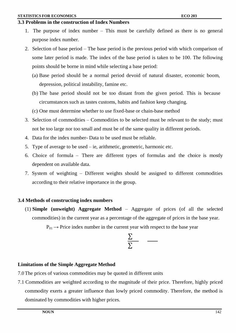
NOUN 142
STATISTICS FOR ECONOMICS ECO 203
3.3 Problems in the construction of Index Numbers
1. The purpose of index number – This must be carefully defined as there is no general
purpose index number.
2. Selection of base period – The base period is the previous period with which comparison of
some later period is made. The index of the base period is taken to be 100. The following
points should be borne in mind while selecting a base period:
(a) Base period should be a normal period devoid of natural disaster, economic boom,
depression, political instability, famine etc.
(b) The base period should not be too distant from the given period. This is because
circumstances such as tastes customs, habits and fashion keep changing.
(c) One must determine whether to use fixed-base or chain-base method
3. Selection of commodities – Commodities to be selected must be relevant to the study; must
not be too large nor too small and must be of the same quality in different periods.
4. Data for the index number- Data to be used must be reliable.
5. Type of average to be used – ie, arithmetic, geometric, harmonic etc.
6. Choice of formula – There are different types of formulas and the choice is mostly
dependent on available data.
7. System of weighting – Different weights should be assigned to different commodities
according to their relative importance in the group.
3.4 Methods of constructing index numbers
(1) Simple (unweight) Aggregate Method – Aggregate of prices (of all the selected
commodities) in the current year as a percentage of the aggregate of prices in the base year.
P01 → Price index number in the current year with respect to the base year
∑
∑
Limitations of the Simple Aggregate Method
7.0 The prices of various commodities may be quoted in different units
7.1 Commodities are weighted according to the magnitude of their price. Therefore, highly priced
commodity exerts a greater influence than lowly priced commodity. Therefore, the method is
dominated by commodities with higher prices.
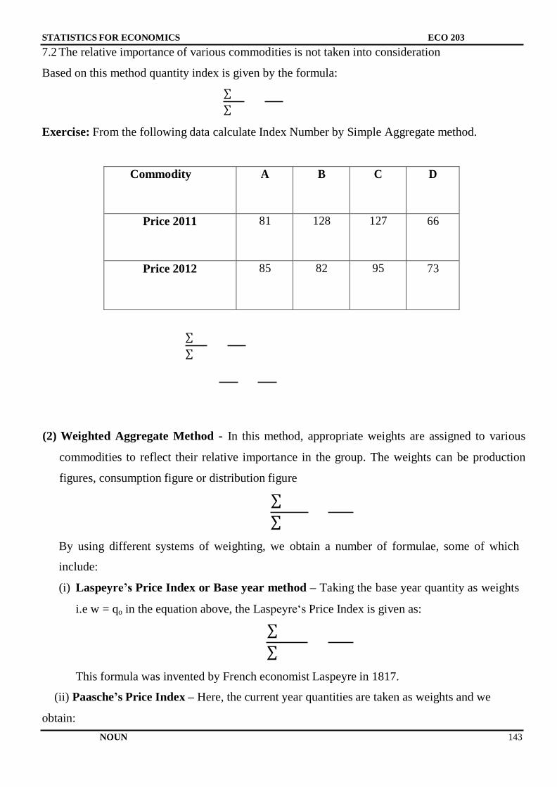
NOUN 143
STATISTICS FOR ECONOMICS ECO 203
7.2 The relative importance of various commodities is not taken into consideration
Based on this method quantity index is given by the formula:
∑
∑
Exercise: From the following data calculate Index Number by Simple Aggregate method.
Commodity A B C D
Price 2011 81 128 127 66
Price 2012 85 82 95 73
∑
∑
(2) Weighted Aggregate Method - In this method, appropriate weights are assigned to various
commodities to reflect their relative importance in the group. The weights can be production
figures, consumption figure or distribution figure
∑
∑
By using different systems of weighting, we obtain a number of formulae, some of which
include:
(i) Laspeyre’s Price Index or Base year method – Taking the base year quantity as weights
i.e w = qo in the equation above, the Laspeyre‘s Price Index is given as:
∑
∑
This formula was invented by French economist Laspeyre in 1817.
(ii) Paasche’s Price Index – Here, the current year quantities are taken as weights and we
obtain:
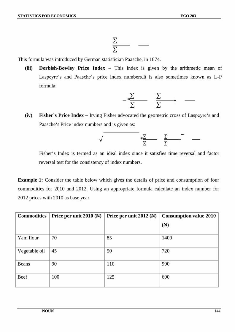
NOUN 144
STATISTICS FOR ECONOMICS ECO 203
∑
∑
This formula was introduced by German statistician Paasche, in 1874.
(iii) Dorbish-Bowley Price Index – This index is given by the arithmetic mean of
Laspeyre‘s and Paasche‘s price index numbers.It is also sometimes known as L-P
formula:
∑ ∑ *∑ ∑
+
(iv) Fisher’s Price Index – Irving Fisher advocated the geometric cross of Laspeyre‘s and
Paasche‘s Price index numbers and is given as:
∑ ∑
√ * + ∑ ∑
Fisher‘s Index is termed as an ideal index since it satisfies time reversal and factor
reversal test for the consistency of index numbers.
Example 1: Consider the table below which gives the details of price and consumption of four
commodities for 2010 and 2012. Using an appropriate formula calculate an index number for
2012 prices with 2010 as base year.
Commodities Price per unit 2010 (N) Price per unit 2012 (N) Consumption value 2010
(N)
Yam flour 70 85 1400
Vegetable oil 45 50 720
Beans 90 110 900
Beef 100 125 600
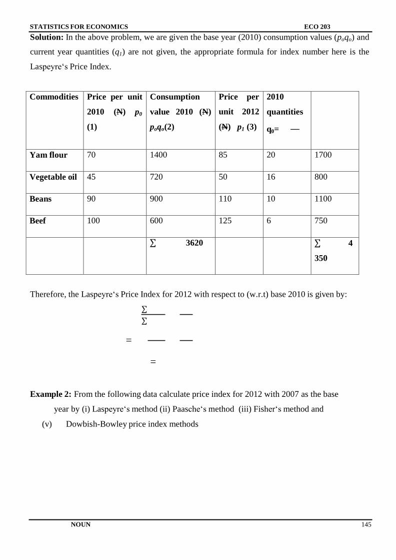
NOUN 145
STATISTICS FOR ECONOMICS ECO 203
Solution: In the above problem, we are given the base year (2010) consumption values (poqo) and
current year quantities (q1) are not given, the appropriate formula for index number here is the
Laspeyre‘s Price Index.
Commodities Price per unit
2010 (N) p0
(1)
Consumption
value 2010 (N)
poqo(2)
Price per
unit 2012
(N) p1 (3)
2010
quantities
q0=
Yam flour 70 1400 85 20 1700
Vegetable oil 45 720 50 16 800
Beans 90 900 110 10 1100
Beef 100 600 125 6 750
∑ 3620
∑ 4
350
Therefore, the Laspeyre‘s Price Index for 2012 with respect to (w.r.t) base 2010 is given by:
∑
∑
=
=
Example 2: From the following data calculate price index for 2012 with 2007 as the base
year by (i) Laspeyre‘s method (ii) Paasche‘s method (iii) Fisher‘s method and
(v) Dowbish-Bowley price index methods
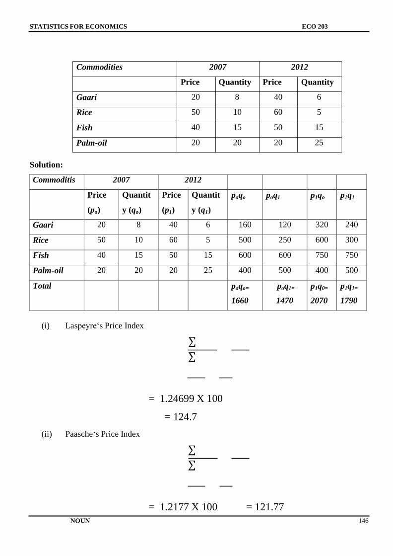
NOUN 146
STATISTICS FOR ECONOMICS ECO 203
Commodities 2007 2012
Price Quantity Price Quantity
Gaari 20 8 40 6
Rice 50 10 60 5
Fish 40 15 50 15
Palm-oil 20 20 20 25
Solution:
Commoditis 2007 2012
Price
(po)
Quantit
y (qo)
Price
(p1)
Quantit
y (q1)
poqo poq1 p1qo p1q1
Gaari 20 8 40 6 160 120 320 240
Rice 50 10 60 5 500 250 600 300
Fish 40 15 50 15 600 600 750 750
Palm-oil 20 20 20 25 400 500 400 500
Total poqo=
1660
poq1=
1470
p1q0=
2070
p1q1=
1790
(i) Laspeyre‘s Price Index
∑
∑
(ii) Paasche‘s Price Index
= 1.24699 X 100
= 124.7
∑ ∑
= 1.2177 X 100 = 121.77
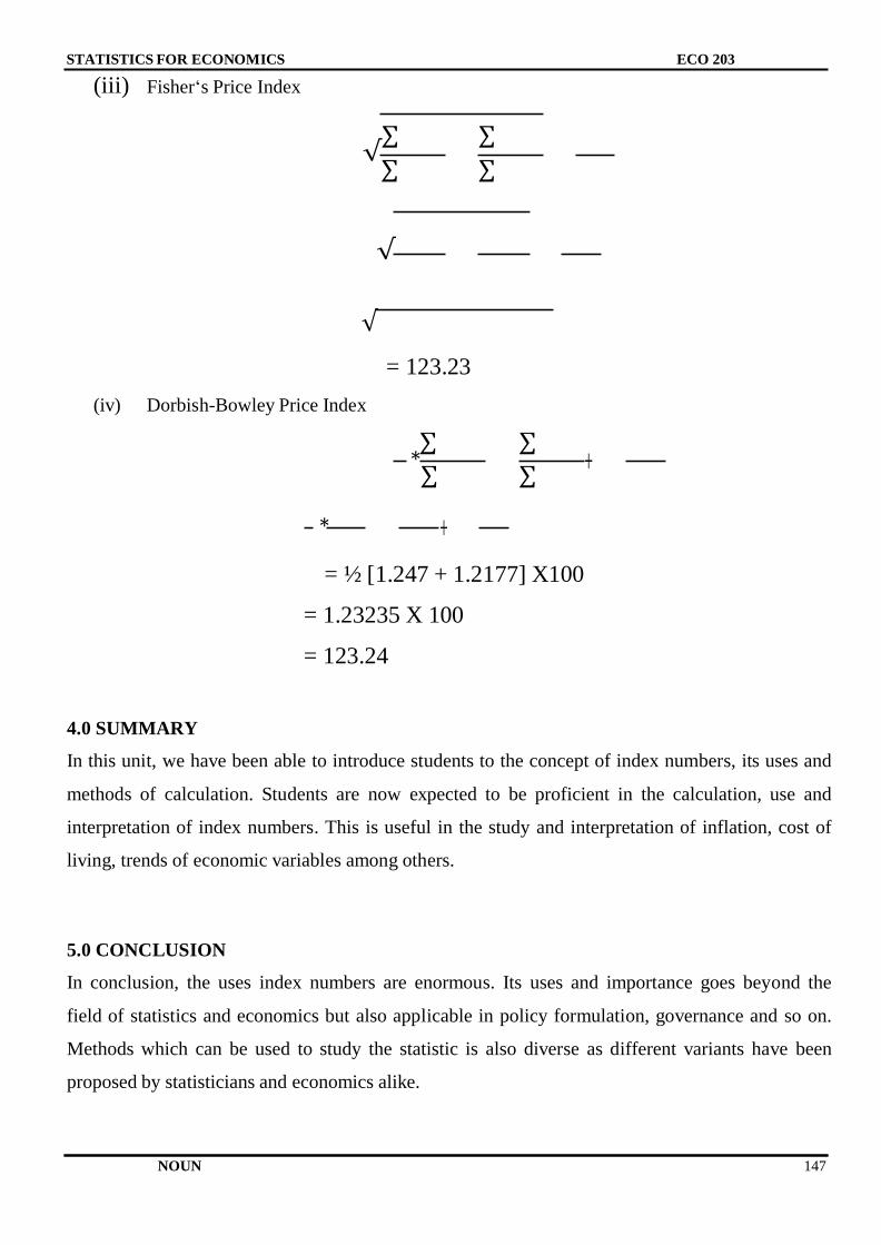
NOUN 147
STATISTICS FOR ECONOMICS ECO 203
(iii) Fisher‘s Price Index
∑ ∑ √ ∑ ∑
√
√
(iv) Dorbish-Bowley Price Index
= 123.23
∑ ∑ *∑ ∑
+
* +
= ½ [1.247 + 1.2177] X100
= 1.23235 X 100
= 123.24
4.0 SUMMARY
In this unit, we have been able to introduce students to the concept of index numbers, its uses and
methods of calculation. Students are now expected to be proficient in the calculation, use and
interpretation of index numbers. This is useful in the study and interpretation of inflation, cost of
living, trends of economic variables among others.
5.0 CONCLUSION
In conclusion, the uses index numbers are enormous. Its uses and importance goes beyond the
field of statistics and economics but also applicable in policy formulation, governance and so on.
Methods which can be used to study the statistic is also diverse as different variants have been
proposed by statisticians and economics alike.

NOUN 148
STATISTICS FOR ECONOMICS ECO 203
6.0 TUTOR-MARKED ASSIGNMENT
1. Calculate Price index number of the year2010 with 2000 as the base year from the following
data using:
(i) Laspeyre‘s
(ii) Pasche‘s
(iii) Dorbish-Bowley and
(iv) Fisher‘s formulae
Commodity 2000 2010
Unit Price (N) Value (N) Quantity consume Value (N)
Rice Kg 20 3000 320 3520
Gaari Kg 24 2160 200 2600
Cloth Yards 30 1800 120 1920
Sugar Packets 18 900 80 960
2. From the following data construct Fisher‘s ideal index number
Commodity 2003 2013
Price (N) Value (N) Price (N) Value (N)
W 15 150 18 216
X 21 252 30 240
Y 30 240 36 288
Z 12 60 15 90
NOUN 149
STATISTICS FOR ECONOMICS ECO 203
7.0 REFERENCES / FURTHER READING
Gupta S.C. (2011). Fundamentals of Statistics.(6th
Rev. and Enlarged ed.).Mumbai India:
Himalayan Publishing House.
Lucey T. (2002). Quantitative Techniques.(6th
ed.).BookPower
NOUN 150
STATISTICS FOR ECONOMICS ECO 203
UNIT 2: STATISTICAL DATA
1.0 Objectives
2.0 Introduction
3.0 Main Content
4.0 Summary
5.0 Conclusion
6.0 Tutor-Marked Assignment
7.0 References/Further Reading
1.0 OBJECTIVES
The objective of this unit is to make learners appreciate the purpose of statistical tests and data, in
the determinationof whether some hypotheses are extremely unlikely given observed data.
2.0 INTRODUCTION
Statistics is a branch of mathematics that deals with the collection, organization, and analysis of
numerical data and with such problems as experiment design and decision making. Simple forms
of statistics have been used since the beginning of civilization, when pictorial representations or
other symbols were used to record numbers of people, animals, and inanimate objects on skins,
slabs, or sticks of wood and the walls of caves. Before 3000BC the Babylonians used small clay
tablets to record tabulations of agricultural yields and of commodities bartered or sold. The
Egyptians analyzed the population and material wealth of their country before beginning to build
the pyramids in the 31st century BC. The biblical books of Numbers and first Chronicles are
primarily statistical works, the former containing two separate censuses of the Israelites and the
latter describing the material wealth of various Jewish tribes. Similar numerical records existed in
China before 2000BC. The ancient Greeks held censuses to be used as bases for taxation as early
as 594BC. The Roman Empire was the first government to gather extensive data about the
population, area, and wealth of the territories that it controlled.
At present, however, statistics is a reliable means of describing accurately the values of economic,
political, social, psychological, biological, and physical data and serves as a tool to correlate and
NOUN 151
STATISTICS FOR ECONOMICS ECO 203
analyze such data. The work of the statistician is no longer confined to gathering and tabulating
data, but is chiefly a process of interpreting the information. The development of the theory of
probability increased the scope of statistical applications. Much data can be approximated
accurately by certain probability distributions, and the results of probability distributions can be
used in analyzing statistical data. Probability can be used to test the reliability of statistical
inferences and to indicate the kind and amount of data required for a particular problem.
[
3.0 MAIN CONTENT
Types of Data
Data can be classified into types based on different criteria viz:
1. Based on sources – Data can be classified base on the sources from which they are obtained. In
this regards, we have:
(a) Primary data – These are data collected directly from the field of enquiries by the
user(s) or researcher(s) themselves.
Advantages
– They are always relevant to the subject under study because they are collected
primarily for the purpose.
- They are more accurate and reliable
- Provide opportunity for the researcher to interact with study population.
- Information on other relevant issues can be obtained
Disadvantages
– Always costly to collect
- Inadequate cooperation from the study population
- Wastes a lot of time and energy
(b) Secondary Data: These are data which have been collected by someone else or some
organization either in published or unpublished forms.
Advantages
- It is easier to get
- It is less expensive

NOUN 152
STATISTICS FOR ECONOMICS ECO 203
Disadvantages
- May not completely meet the need of the research athand because it was not
collected primarily for particular purpose
- There is always a problem of missing periods
2.Classification based on form of the data: Sometimes, data are classified based on the form of
the data at hand and may be classified as:
(a) Cross-sectional data – These are data collected for cross-section of subjects
(population under study) at a time. For example, data collected on a cross-section of
household on demand for recharge card for the month of August 2013.
(b) Time-series data – These are data collected on a particular variable or set of
variables over time e.g a set Nigeria‘s Gross Domestic Product (GDP) values form
1970 to2012.
(c) Panel Data – These combine the features of cross-sectional and time-series data. They
are type of data collected from the same subjects over time. For example, a set of data
collected on monthly recharge card expenditure from about 100 households in Lagos
from January to December 2013 will form a panel data.
Note that Social and Economic data of national importance are collected routinely as by-product
of governmental activities e.g. information on trade, wages, prices, education, health, crime, aids
and grants etc.
Sources of Data
1. Source of Primary data:
(i) Census
(ii) Surveys
2. Sources of Secondary data:
(i) Publications of the Federal Bureau of statistics
(ii) Publications of Central Bank of Nigeria
(iii) Publications of National population commission
NOUN 153
STATISTICS FOR ECONOMICS ECO 203
(iv) Nigerian Custom Service
(v) Nigeria Immigration Service
(vi) Nigerian Port Authority
(vi) Federal and State Ministries, Departments and Agencies
Some of the publications referred to above are: (i)
Annual Digest of statistics (by NBS)
(ii) Annual Abstract of statistics (by NBS)
(iii) Economic and Financial Review (by CBN)
(iv) Population of Nigeria (by NPC)
4.0 SUMMARY
This unit has acquainted you with the transformation of the processed data into statistics and steps
in the statistical cycle. The transformation involves analysis and interpretation of data to identify
important characteristics of a population and provide insights into the topic being investigated.
5.0 CONCLUSION
Here, a further aim of statistical data and testing is shown to you to quantify evidence against a
particular hypothesis being true. You were able to think of it as testing to guide research. We
believe a certain statement may be true and want to work out whether it is worth investing time
investigating it. Therefore, we look at the opposite of this statement. If it is quite likely then
further study would seem to not make sense. However if it is extremely unlikely then further
study would make sense.
6.0 TUTOR-MARKED ASSIGNMENT
1. Distinguish between primary and secondary data
2. What are the advantages of primary data
3. List 4 source of secondary data you know
4. Distinguish between cross-sectional and panel data
NOUN 154
STATISTICS FOR ECONOMICS ECO 203
7.0 REFERENCES / FURTHER READINGS
Frankfort-Nachmias C. and Nachmias D. (2009).Research in the Social Sociences.(5th
ed.).Hodder
Education.
Gupta S.C. (2011). Fundamentals of Statistics.(6th
Rev. and Enlarged ed.). Mumbai India:
Himalayan Publishing House
Microsoft ® Encarta ® 2009. © 1993-2008 Microsoft Corporation.
NOUN 155
STATISTICS FOR ECONOMICS ECO 203
UNIT 3: SAMPLE AND SAMPLING TECHNIQUES
CONTENTS
1.0 Objectives
2.0 Introduction
3.0 Main Content
4.0 Summary
5.0 Conclusion
6.0 Tutor-Marked Assignment
7.0 References/Further Reading
1.0 OBJECTIVES
The objective of this unit is to make learners understand the importance of data collection to aid
planning and decision making
2.0 INTRODUCTION
Researchers collect data in order to test hypotheses and to provide empirical support for
explanations and predictions. Once investigators have constructed their measuring instrument in
order to collect sufficient data pertinent to the research problem, the subsequent explanations and
predictions must be capable of being generalized to be of scientific value. Generalizations are
important not only for testing hypotheses but also for descriptive purposes. Typically,
generalizations are not based on data collected from all the observations, all the respondents, or
the events that are defined by the research problem as this is always not possible or where possible
too expensive to undertake. Instead, researchers use a relatively small number of cases (a sample)
as the bases for making inferences for all the cases (a population).
3.0 MAIN CONTENT
Empirically supported generalizations are usually based on partial information because it is often
impossible, impractical, or extremely expensive to collect data from all the potential units of
analysis covered by the research problem. Researchers can draw precise inferences on all the units
(a set) based on relatively small number of units (a subset) when the subsets accurately represent
the relevant attributes of the whole sets. For example, in a study of patronage of campus
NOUN 156
STATISTICS FOR ECONOMICS ECO 203
photographer among students in a university, it may be very expensive and time consuming to
reach out to all students (some universities have as high as 40,000 students). A careful selection of
relatively small number of students across faculties, departments and levels will possibly give a
representation of the entire student population.
The entire set of relevant units of analysis, or data is called the population. When the data serving
as the basis for generalizations is comprised of a subset of the population, that subset is called a
sample. A particular value of the population, such as the mean income or the level of formal
education, is called a parameter; its counterpart in the sample is termed the statistic. The major
objective of sampling theory is to provide accurate estimates of unknown values of the parameters
from sample statistics that can be easily calculated. To accurately estimate unknown parameters
from known statistics, researchers have to effectively deal with three major problems:
(1) the definition of the population,
(2) the sample design, and
(3) the size of the sample.
Population
Methodologically, a population is the ―aggregate of all cases that conform to some designated set
of specifications‖. For example, a population may be composed of all the residents in a specific
neighbourhood, legislators, houses, records, and so on. The specific nature of the population
depends on the research problem. If you are investigating consumer behaviour in a particular city,
you might define the population as all the households in that city. Therefore, one of the first
problems facing a researcher who wishes to estimate a population value from a sample value is
how to determine the population involved.
The Sampling Unit
A single member of a sampling population (e.g. a household) is referred to as a sampling unit.
Usually sampling units have numerous attributes, one or more of which are relevant to the
research problem. The major attribute is that it must possess the typical characteristics of the study
population. A sampling unit is not necessarily an individual. It can be an event, a university, a city
or a nation.
NOUN 157
STATISTICS FOR ECONOMICS ECO 203
Sampling Frame
Once researchers have defined the population, they draw a sample that adequately represents that
population. The actual procedures involve in selecting a sample from a sample frame comprised
of a complete listing of sampling units. Ideally, the sampling frame should include all the
sampling units in the population. In practice, a physical list rarely exists; researchers usually
compile a substitute list and they should ensure that there is a high degree of correspondence
between a sampling frame and the sampling population. The accuracy of a sample depends, first
and foremost, on the sampling frame. Indeed, every aspect of the sample design – the population
covered, the stages of sampling, and the actual selection process – is influenced by the sampling
frame. Prior to selecting a sample, the researcher has to evaluate the sampling frame for potential
problems.
Sample Design
The essential requirement of any sample is that it be as representative as possible of the
population from which it is drawn. A sample is considered to be representative if the analyses
made using the researcher‘s sampling units produce results similar to those that would be obtained
had the researcher analyzed the entire population.
Probability and Non-probability Sampling
In modern sampling theory, a basic distinction is made between probability and non-probability
sampling. The distinguishing characteristic of probability sampling is that for each sampling unit
of the population, you can specify the probability that the unit will be included in the sample. In
the simplest case, all the units have the same probability of being included in the sample. In non-
probability sampling, there is no assurance that every unit has some chance of being included.
A well – designed sample ensures that if a study were to be repeated on a number of different
samples drawn from a given population, the findings from each sample would not differ from the
population parameters by more than a specified amount. A probability sample design makes it
possible for researchers to estimate the extent to which the findings based on one sample are
likely to differ from what they would have found by studying the entire population. When a
researcher is using a probability sample design, it is possible for him or her to estimate the
population‘s parameters on the basis of the sample statistics calculated.
NOUN 158
STATISTICS FOR ECONOMICS ECO 203
Non-probability Sample Designs
Three major designs utilizing non-probability samples have been employed by social scientists:
convenience samples, purposive samples, and quota samples.
Convenience sampling: Researchers obtain a convenience sample by selecting whatever
sampling units are conveniently available. Thus a University professor may select students in a
class; or a researcher may take the first 200 people encountered on the street who are willing to be
interviewed. The researcher has no way of estimating the representativeness of convenience
sample, and therefore cannot estimate the population‘s parameters.
Purposive sampling: With purposive samples (occasionally referred to as judgment samples),
researchers select sampling units subjectively in an attempt to obtain a sample that appears to be
representative of the population. In order words, the chance that a particular sampling unit will
selected for the sample depends on the subjective judgment of the researcher. At times, the main
reason for selecting a unit in purposive sampling is the possession of pre-determined
characteristic(s) which may be different from that the main population. For example, in a study of
demand preference for cigarette brands in a city, researcher will need to select smokers
purposively.
Quota sampling: The chief aim of quota sample is to select a sample that is as similar as possible
to the sampling population. For example, if it is known that the population has equal numbers of
males and females, the researcher selects an equal numbers of males and females in the sample. In
quota sampling, interviewers are assigned quota groups characterized by specific variables such as
gender, age, place of residence, and ethnicity.
Probability Sample Designs
Four common designs of probability samples are simple random sampling, systematic sampling,
stratified sampling, and cluster sampling.
Simple random sampling – is the basic probability sampling design, and it is incorporated into
all the more elaborate probability sampling designs. Simple random sampling is a procedure that
gives each of the total sampling units of the population an equal and known nonzero probability of
being selected. For example, when you toss a perfect coin, the probability that you will get a head
or a tail is equal and known (50 percent), and each subsequent outcome is independent of the
previous outcomes.
NOUN 159
STATISTICS FOR ECONOMICS ECO 203
Random selection procedures ensure that every sampling unit of the population has an equal and
known probability of being included in the sample; this probability is n/N, where n stands for the
size of the sample and N for the size of the population. For example if we are interested in
selection 60 household from a population of 300 households using simple random sampling, the
probability of a particular household being selected is 60/300 = 1/5.
Systematic Sampling: It consists of selecting every kth
sampling unit of the population after the
first sampling unit is selected at random from the total of sampling units. Thus if you wish to
select a sample of 100 persons from total population of 10,000, you would take every hundredth
individual (K=N/n = 10,000/100 = 100). Suppose that the fourteenth person were selected; the
sample would then consist of individuals numbered 14,114, 214, 314, 414, and so on. Systematic
sampling is more convenient than simple random sampling. Systematic samples are also more
amenable for use with very large populations or when large samples are to be selected.
Stratified Sampling:Researchers use this method, primarily to ensure that different groups of
population are adequately represented in the sample. This is to increase their level of accuracy
when estimating parameters. Furthermore, all other things being equal, stratified sampling
considerably reduces the cost of execution. The underlying idea in stratified sampling is to use
available information on the population ―to divide it into groups such that the elements within
each group are more alike than are the elements in the population as a whole. That is, you create a
set of homogeneous samples based on the variables you are interested in studying. If a series of
homogenous groups can be sampled in such a way when the samples are combined they constitute
a sample of a more heterogeneous population, you will increase the accuracy of your parameter
estimates.
Cluster sampling: it is frequently used in large-scale studies because it is the least expensive
sample design. Cluster sampling involves first selecting large groupings, called clusters, and then
selecting the sampling units from the clusters. The clusters are selected by a simple random
sample or a stratified sample. Depending on the research problem, researchers can include all the
sampling units in these clusters in the sample or make a selection within the clusters using simple
or stratified sampling procedures.
NOUN 160
STATISTICS FOR ECONOMICS ECO 203
Sample size
A sample is any subset of sampling units from a population. A subset is any combination of
sampling units that does not include the entire set of sampling units that has been defined as the
population. A sample may include only one sampling unit, or any number in between.
There are several misconceptions about the necessary size of a sample. One is that the sample size
must be certain proportion (often set as 5 percent) of the population; another is that the sample
should total about 2000; still another is that any increase in the sample size will increase the
precision of the sample results. These are faulty notions because they do not derive from the
sampling theory. To estimate the adequate size of the sample properly, researchers need to
determine what level of accuracy is expected of their estimates; that is, how large a standard error
is acceptable.
Standard error
Some people called it error marginorsampling error. The concept of standard error is central to
sampling theory and to determining the size of a sample. It is one of the statistical measures that
indicate how closely the sample results reflect the true value of a parameter.
Methods of data collection
There are three methods of data collection with survey and these are mail questionnaires, personal
interviews, and telephone interviews.
Mail questionnaire: It is an impersonal survey method. Here, survey instrument (the
questionnaire) is mailed to the selected respondents and the questionnaires are mailed back to the
researcher after the respondents must have filled it up. This is very common in developed
countries where the citizens appreciate the relevance of data and research. Under certain
conditions and for a number of research purposes, an impersonal method of data collection can be
useful.
NOUN 161
STATISTICS FOR ECONOMICS ECO 203
Advantages and disadvantages of mail questionnaires
Advantages
The cost is low compared to others
Biasing error is reduced because respondents are not influenced by interviewed
characteristics or techniques.
Questionnaires provide a high degree of anonymity for respondents. This is especially
important when sensitive issues are involved.
Respondents have time to think about their answers and /or consult other sources.
Questionnaires provide wide access to geographically dispersed samples at low cost
Disadvantages
Questionnaires require simple, easily understood questions and instructions
Mail questionnaires do not offer researchers the opportunity to probe for additional
information or to clarify answers.
Researchers cannot control who fills out the questionnaire.
Response rate are low
Factors affecting the response rate of mail questionnaires
Researchers use various strategies to overcome the difficulty of securing an acceptable response
rate to mail questionnaires and to increase the response rate.
Sponsorship: The sponsorship of a questionnaire motivates the respondents to fill the
questionnaires and return them. Therefore, investigators must include information on
sponsorship, usually in the cover letter accompanying the questionnaire.
Inducement to response: Researchers who use mail surveys must appeal to the respondents
and persuade them that they should participate by filling out the questionnaires and mailing
them back. For example, a student conducting a survey for a class project may mention that
his or her grade may be affected by the response to the questionnaire.
Questionnaire format and methods of mailing- Designing a mail questionnaire involves
several considerations: typography, colour, and length and type of cover letter.
NOUN 162
STATISTICS FOR ECONOMICS ECO 203
Personal interview
The personal interview is a face-to-face, interpersonal role situation in which an interviewer asks
respondents question designed to elicits answers pertinent to the research hypotheses. The
questions, their wording, and their sequence define the structure of the interview.
Advantages of personal interview
Flexibility: The interview allows great flexibility in the questioning process, and the greater
the flexibility, the less structure the interview. Some interviews allow the interviewer to
determine the wording of the questions, to clarify terms that are unclear, to control the
order in which the question are presented, and to probe for additional information and
details.
Control of the interview situation: An interviewer can ensure that the respondents answer
the questions in the appropriate sequence or that they answer certain questions before they
ask subsequent questions.
High response rate: The personal interview results in a higher response rate than the mail
questionnaire.
Fuller information: An interviewer can collect supplementary information about
respondents. This may include background information, personal characteristics and their
environment that can aid the researcher in interpreting the results.
Disadvantages of the personal interview
Higher cost: The cost of interview studies is significantly higher than that of mail
survey. Costs are involved in selecting, training, and supervising interviewers; in
paying them; and in the travel and time required to conduct interviews.
Interviewer bias: The very flexibility that is the chief advantage of interviews leaves
room for the interviewer‘s personal influence and bias.
Lack of anonymity: The interview lacks the anonymity of the mail questionnaire. Often
the interviewer knows all or many of the potential respondents (their names, addresses,
and telephone numbers). Thus respondents may feel threatened or intimidated by the
interviewer, especially if a respondent is sensitive to the topic or some of the questions.
NOUN 163
STATISTICS FOR ECONOMICS ECO 203
Telephone interview
It is also called telephone survey, and can be characterised as a semi-personal method of
collecting information. In comparison, the telephone is convenient, and it produces a very
significant cost saving.
Advantages of Telephone interview
Moderate cost
Speed: Telephone interviews can reach a large of respondents in a short time.
Interviewers can code data directly into computers, which can later compile the
data.
High response rate: Telephone interviews provide access to people who might be
unlikely to reply to a mail questionnaire or refuse a personal interview.
Quality: High quality data can be collected when interviewers are centrally located
and supervisors can ensure that questions are being asked correctly and answers
are recorded properly.
Disadvantages of Telephone interview
Reluctant to discuss sensitive topics: Respondents may be resistant to discuss some
issues over the phone.
The ―broken off‖ interview: Respondents can terminate the interview before it is
completed.
Less information Interviewers cannot provide supplemental information about the
respondents‘ characteristics or environment.
4.0 SUMMARY
You now would be able to discern that a sample is a subset of a population selected to meet
specific objectives. And also familiar with the guiding principle and sampling techniques in
selecting a sample, is that it must, as far as possible have the essential characteristics of the target
population
NOUN 164
STATISTICS FOR ECONOMICS ECO 203
5.0 CONCLUSION
This unit has relayed to you that a well-chosen sample can usually provide reliable information
about the whole of the population to any desired degree of accuracy. In some instances sampling
is an alternative to a complete census, and may be preferable mainly because of its cheapness and
convenience.
6.0 TUTOR-MARKED ASSIGNMENT
1. Explain three non-probability sampling methods
2. What are the advantages of telephone interview
3. Is there any disadvantage(s) in personal interview method of data collection
7.0 REFERENCES/FURTHER READINGS
Frankfort-Nachmias C. and Nachmias D. (2009).Research in the Social Sociences.(5th
ed.).Hodder
Education.
Gupta S.C (2011). Fundamentals of Statistics.(6th
Rev. and Enlarged ed.). Mumbai India:
Himalayan Publishing House
Esan E. O. and Okafor R. O. (1995) Basic Statistical Methods,(1sted.). Lagos Nigeria: JAS
Publishers, pages 72-89

![NATIONAL OPEN UNIVERSITY OF NIGERIAnouedu.net/sites/default/files/2017-03/COP 311 MAIN TEXT.pdfNATIONAL OPEN UNIVERSITY OF NIGERIA ... [TMA]. The sources of ... to provide relevant](https://img.pdfslide.us/doc/110x75/5aacb5d47f8b9a693f8d673f/national-open-university-of-311-main-textpdfnational-open-university-of-nigeria.jpg)