National Longitudinal Study of Adolescent Health

Obesity and Neighborhood Environment

Penny Gordon-Larsen

❖ ❖ ❖ ❖ ❖

Carolina Population Center University of North Carolina at Chapel Hill

October 2009

This research was funded by National Institutes of Health (National Institute of Child Health and Human Development grants R01 HD39183, R01 HD041375, and K01 HD044263; National Institute of Diabetes

and Digestive and Kidney Diseases grant DK56350; and National Institute on Environmental Health Sciences grant P30ES10126), National Institute of Aging NIA: K07 AG001015 and P30 AG024376; and a

cooperative agreement with the Centers for Disease Control and Prevention (CDC SIP No. 5-00).

Persons interested in obtaining data files from Add Health should contact Add Health, Carolina Population Center, 123 W. Franklin Street, Chapel Hill, NC 27516-2524 (addhealth@unc.edu)

i

Add Health Obesity and Neighborhood Environment

Table of Contents

Table of Contents ........................................................................................................................................... i

Overview ....................................................................................................................................................... 1

Database Creation ........................................................................................................................................ 1

1. Ascertainment of residential locations .............................................................................................. 1

2. Building the spatial database ............................................................................................................ 2

Defining the geographic scope of the database.................................................................................... 2

Compiling the environment data ........................................................................................................... 3

Spatial analytical methods .................................................................................................................... 4

Data quality ........................................................................................................................................... 5

3. Creation of respondent-specific environment measures .................................................................. 6

Neighborhood definitions ...................................................................................................................... 6

Environment measures ......................................................................................................................... 7

4. Linkage to individual-level data ......................................................................................................... 8

Overview of each dataset .............................................................................................................................. 8

ACCRA ...................................................................................................................................................... 8

Census ...................................................................................................................................................... 9

Climate ...................................................................................................................................................... 9

Coastline ................................................................................................................................................... 9

Connectivity ............................................................................................................................................... 9

Crime ......................................................................................................................................................... 9

Distance to School .................................................................................................................................. 10

Employment ............................................................................................................................................ 10

Geocode Source ..................................................................................................................................... 10

Land Cover .............................................................................................................................................. 10

Length of Day .......................................................................................................................................... 11

Mean Slope Angle ................................................................................................................................... 11

Mobility Indicator ..................................................................................................................................... 11

Parks Distance and Area ........................................................................................................................ 11

Pollution................................................................................................................................................... 12

Proportional Block Group Population and Area ...................................................................................... 12

Resource Counts and Distance (RCD) Measures .................................................................................. 12

Road Type Length ................................................................................................................................... 12

RUCA ...................................................................................................................................................... 13

Shopping Malls ........................................................................................................................................ 13

Urbanized Area Distance ........................................................................................................................ 13

Urban Traffic Congenstion ...................................................................................................................... 13

ii

Weather ................................................................................................................................................... 13

Web Parks ............................................................................................................................................... 14

References .................................................................................................................................................. 15

Acknowledgement ....................................................................................................................................... 16

Appendix ..................................................................................................................................................... 17

Note: Not all files have been released as of October 2009.

1

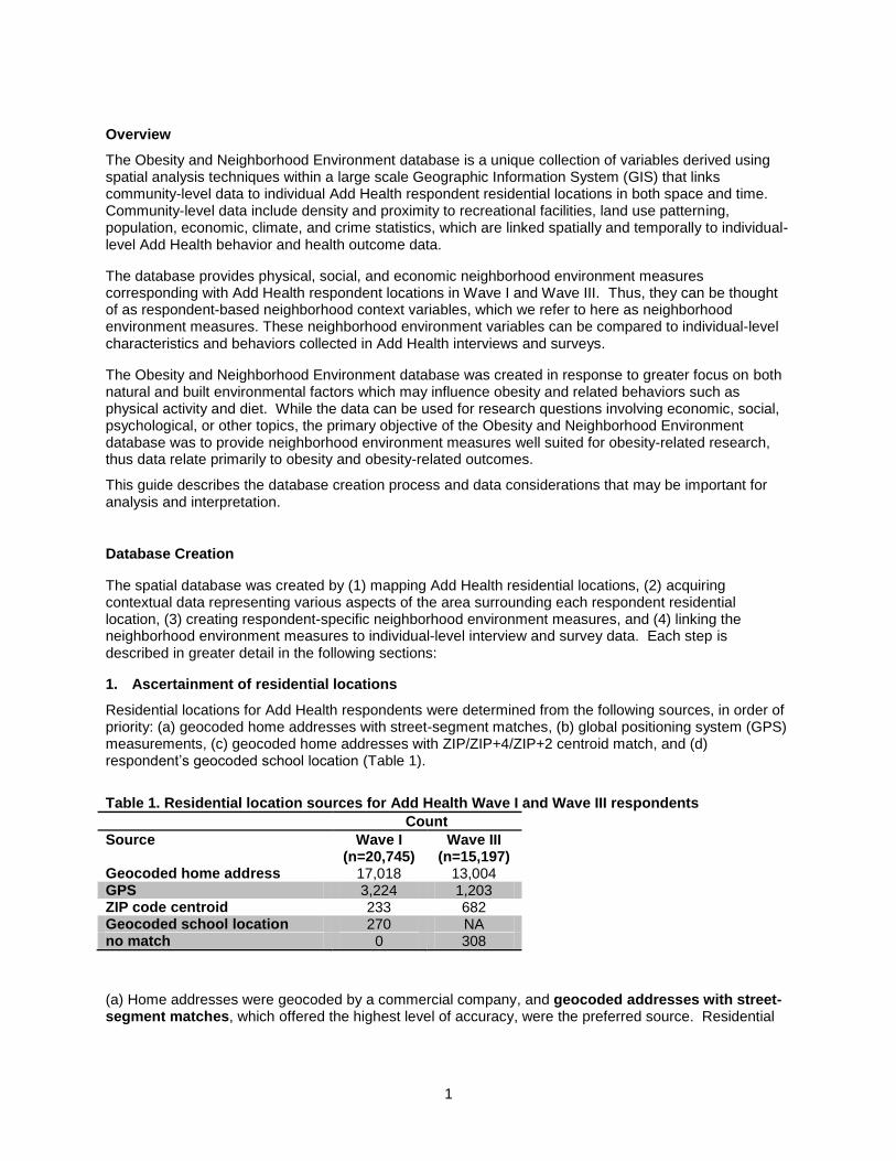
Overview

The Obesity and Neighborhood Environment database is a unique collection of variables derived using spatial analysis techniques within a large scale Geographic Information System (GIS) that links community-level data to individual Add Health respondent residential locations in both space and time. Community-level data include density and proximity to recreational facilities, land use patterning, population, economic, climate, and crime statistics, which are linked spatially and temporally to individual-level Add Health behavior and health outcome data.

The database provides physical, social, and economic neighborhood environment measures corresponding with Add Health respondent locations in Wave I and Wave III. Thus, they can be thought of as respondent-based neighborhood context variables, which we refer to here as neighborhood environment measures. These neighborhood environment variables can be compared to individual-level characteristics and behaviors collected in Add Health interviews and surveys.

The Obesity and Neighborhood Environment database was created in response to greater focus on both natural and built environmental factors which may influence obesity and related behaviors such as physical activity and diet. While the data can be used for research questions involving economic, social, psychological, or other topics, the primary objective of the Obesity and Neighborhood Environment database was to provide neighborhood environment measures well suited for obesity-related research, thus data relate primarily to obesity and obesity-related outcomes.

This guide describes the database creation process and data considerations that may be important for analysis and interpretation.

Database Creation

The spatial database was created by (1) mapping Add Health residential locations, (2) acquiring contextual data representing various aspects of the area surrounding each respondent residential location, (3) creating respondent-specific neighborhood environment measures, and (4) linking the neighborhood environment measures to individual-level interview and survey data. Each step is described in greater detail in the following sections:

1. Ascertainment of residential locations

Residential locations for Add Health respondents were determined from the following sources, in order of priority: (a) geocoded home addresses with street-segment matches, (b) global positioning system (GPS) measurements, (c) geocoded home addresses with ZIP/ZIP+4/ZIP+2 centroid match, and (d) respondent’s geocoded school location (Table 1).

Table 1. Residential location sources for Add Health Wave I and Wave III respondents

Count

Source Wave I (n=20,745)

Wave III (n=15,197)

Geocoded home address 17,018 13,004 GPS 3,224 1,203 ZIP code centroid 233 682 Geocoded school location 270 NA no match 0 308

(a) Home addresses were geocoded by a commercial company, and geocoded addresses with street-segment matches, which offered the highest level of accuracy, were the preferred source. Residential

2

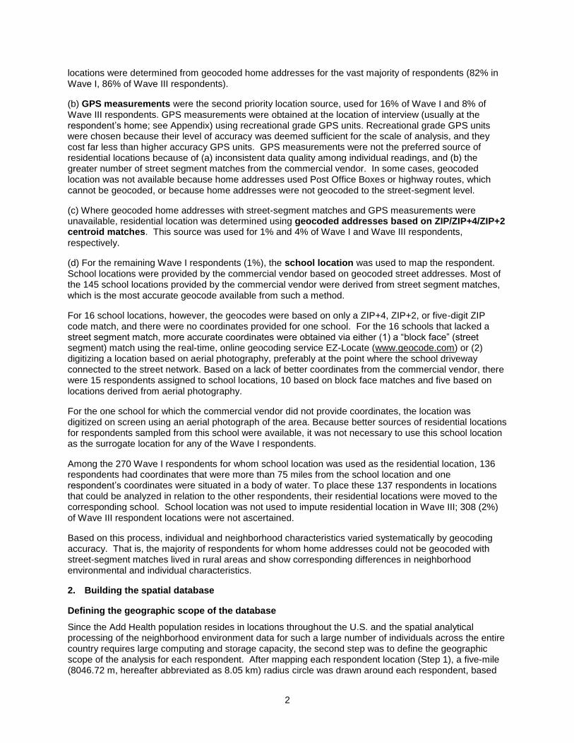
locations were determined from geocoded home addresses for the vast majority of respondents (82% in Wave I, 86% of Wave III respondents).

(b) GPS measurements were the second priority location source, used for 16% of Wave I and 8% of Wave III respondents. GPS measurements were obtained at the location of interview (usually at the respondent’s home; see Appendix) using recreational grade GPS units. Recreational grade GPS units were chosen because their level of accuracy was deemed sufficient for the scale of analysis, and they cost far less than higher accuracy GPS units. GPS measurements were not the preferred source of residential locations because of (a) inconsistent data quality among individual readings, and (b) the greater number of street segment matches from the commercial vendor. In some cases, geocoded location was not available because home addresses used Post Office Boxes or highway routes, which cannot be geocoded, or because home addresses were not geocoded to the street-segment level.

(c) Where geocoded home addresses with street-segment matches and GPS measurements were unavailable, residential location was determined using geocoded addresses based on ZIP/ZIP+4/ZIP+2 centroid matches. This source was used for 1% and 4% of Wave I and Wave III respondents,

respectively.

(d) For the remaining Wave I respondents (1%), the school location was used to map the respondent. School locations were provided by the commercial vendor based on geocoded street addresses. Most of the 145 school locations provided by the commercial vendor were derived from street segment matches, which is the most accurate geocode available from such a method.

For 16 school locations, however, the geocodes were based on only a ZIP+4, ZIP+2, or five-digit ZIP code match, and there were no coordinates provided for one school. For the 16 schools that lacked a street segment match, more accurate coordinates were obtained via either (1) a “block face” (street segment) match using the real-time, online geocoding service EZ-Locate (www.geocode.com) or (2) digitizing a location based on aerial photography, preferably at the point where the school driveway connected to the street network. Based on a lack of better coordinates from the commercial vendor, there were 15 respondents assigned to school locations, 10 based on block face matches and five based on locations derived from aerial photography.

For the one school for which the commercial vendor did not provide coordinates, the location was digitized on screen using an aerial photograph of the area. Because better sources of residential locations for respondents sampled from this school were available, it was not necessary to use this school location as the surrogate location for any of the Wave I respondents.

Among the 270 Wave I respondents for whom school location was used as the residential location, 136 respondents had coordinates that were more than 75 miles from the school location and one respondent’s coordinates were situated in a body of water. To place these 137 respondents in locations that could be analyzed in relation to the other respondents, their residential locations were moved to the corresponding school. School location was not used to impute residential location in Wave III; 308 (2%) of Wave III respondent locations were not ascertained.

Based on this process, individual and neighborhood characteristics varied systematically by geocoding accuracy. That is, the majority of respondents for whom home addresses could not be geocoded with street-segment matches lived in rural areas and show corresponding differences in neighborhood environmental and individual characteristics.

2. Building the spatial database

Defining the geographic scope of the database

Since the Add Health population resides in locations throughout the U.S. and the spatial analytical processing of the neighborhood environment data for such a large number of individuals across the entire country requires large computing and storage capacity, the second step was to define the geographic scope of the analysis for each respondent. After mapping each respondent location (Step 1), a five-mile (8046.72 m, hereafter abbreviated as 8.05 km) radius circle was drawn around each respondent, based

3

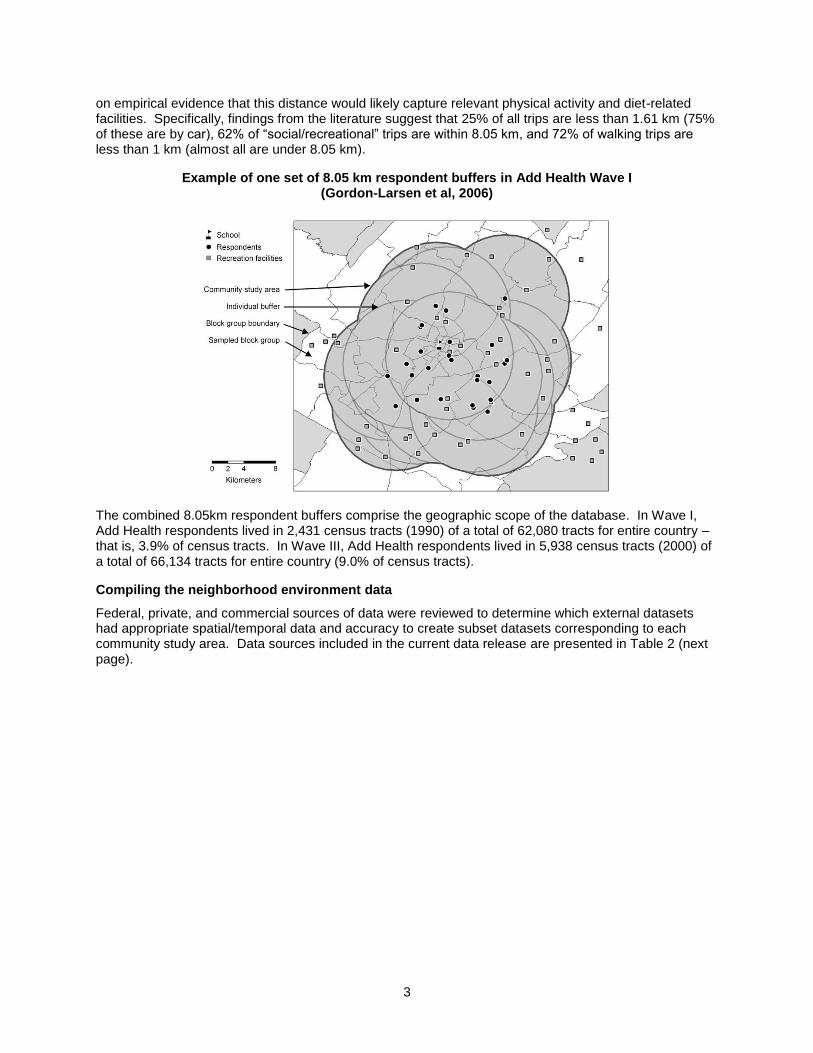
on empirical evidence that this distance would likely capture relevant physical activity and diet-related facilities. Specifically, findings from the literature suggest that 25% of all trips are less than 1.61 km (75% of these are by car), 62% of “social/recreational” trips are within 8.05 km, and 72% of walking trips are less than 1 km (almost all are under 8.05 km).

Example of one set of 8.05 km respondent buffers in Add Health Wave I (Gordon-Larsen et al, 2006)

The combined 8.05km respondent buffers comprise the geographic scope of the database. In Wave I, Add Health respondents lived in 2,431 census tracts (1990) of a total of 62,080 tracts for entire country – that is, 3.9% of census tracts. In Wave III, Add Health respondents lived in 5,938 census tracts (2000) of a total of 66,134 tracts for entire country (9.0% of census tracts).

Compiling the neighborhood environment data

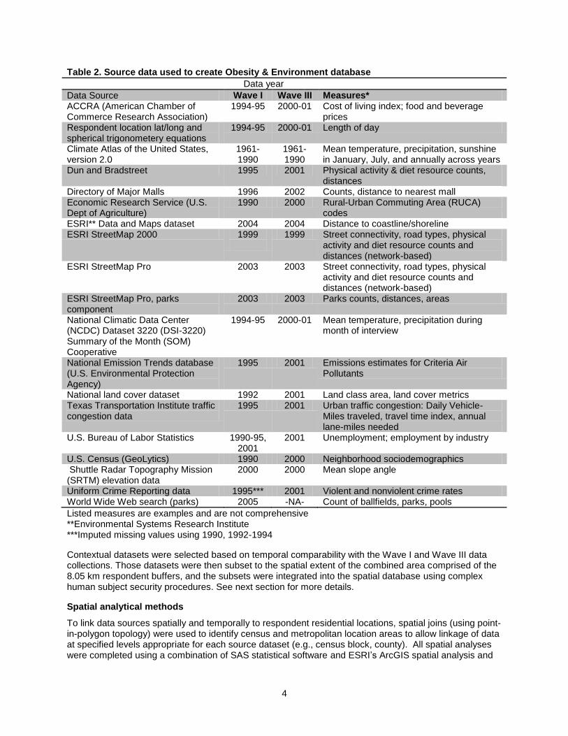
Federal, private, and commercial sources of data were reviewed to determine which external datasets had appropriate spatial/temporal data and accuracy to create subset datasets corresponding to each community study area. Data sources included in the current data release are presented in Table 2 (next page).

4

Table 2. Source data used to create Obesity & Environment database

Data year

Data Source Wave I Wave III Measures* ACCRA (American Chamber of Commerce Research Association)

1994-95 2000-01 Cost of living index; food and beverage prices

Respondent location lat/long and spherical trigonometery equations

1994-95 2000-01 Length of day

Climate Atlas of the United States, version 2.0

1961-1990

1961-1990

Mean temperature, precipitation, sunshine in January, July, and annually across years

Dun and Bradstreet 1995 2001 Physical activity & diet resource counts, distances

Directory of Major Malls 1996 2002 Counts, distance to nearest mall Economic Research Service (U.S. Dept of Agriculture)

1990 2000 Rural-Urban Commuting Area (RUCA) codes

ESRI** Data and Maps dataset 2004 2004 Distance to coastline/shoreline ESRI StreetMap 2000 1999

1999 Street connectivity, road types, physical

activity and diet resource counts and distances (network-based)

ESRI StreetMap Pro 2003 2003 Street connectivity, road types, physical activity and diet resource counts and distances (network-based)

ESRI StreetMap Pro, parks component

2003 2003 Parks counts, distances, areas

National Climatic Data Center (NCDC) Dataset 3220 (DSI-3220) Summary of the Month (SOM) Cooperative

1994-95 2000-01 Mean temperature, precipitation during month of interview

National Emission Trends database (U.S. Environmental Protection Agency)

1995 2001 Emissions estimates for Criteria Air Pollutants

National land cover dataset 1992 2001 Land class area, land cover metrics Texas Transportation Institute traffic congestion data

1995 2001 Urban traffic congestion: Daily Vehicle-Miles traveled, travel time index, annual lane-miles needed

U.S. Bureau of Labor Statistics 1990-95, 2001

2001 Unemployment; employment by industry

U.S. Census (GeoLytics) 1990 2000 Neighborhood sociodemographics Shuttle Radar Topography Mission (SRTM) elevation data

2000 2000 Mean slope angle

Uniform Crime Reporting data 1995*** 2001 Violent and nonviolent crime rates World Wide Web search (parks) 2005 -NA- Count of ballfields, parks, pools

Listed measures are examples and are not comprehensive **Environmental Systems Research Institute ***Imputed missing values using 1990, 1992-1994

Contextual datasets were selected based on temporal comparability with the Wave I and Wave III data collections. Those datasets were then subset to the spatial extent of the combined area comprised of the 8.05 km respondent buffers, and the subsets were integrated into the spatial database using complex human subject security procedures. See next section for more details.

Spatial analytical methods

To link data sources spatially and temporally to respondent residential locations, spatial joins (using point-in-polygon topology) were used to identify census and metropolitan location areas to allow linkage of data at specified levels appropriate for each source dataset (e.g., census block, county). All spatial analyses were completed using a combination of SAS statistical software and ESRI’s ArcGIS spatial analysis and

5

mapping software, customized by our team with programming languages such as AML, Avenue, Python, Visual Basic, NetEngine, and C++ to be able to handle the data volume of this comprehensive and national GIS database.

Data quality Quality control procedures. Many challenges related to integration of data with various scales and spatial coordinates were encountered. To address these issues a series of quality control procedures were undertaken, including:

Exhaustive review of respondent and school locations for Wave I in order to obtain the most accurate geocodes possible before developing any other datasets.

An extensive review of federal, private, and commercial sources of data to determine which datasets had the most appropriate spatial and temporal accuracy for the study area.

A scripted approach for all spatial data processing, which (a) allowed thorough testing and debugging of scripts before execution for all respondents in a wave and (b) provided a well-documented, step-by-step record for quality control purposes.

A specified series of quality control steps for each dataset.

Validation of neighborhood environment data. Despite these measures, all environmental databases are vulnerable to errors due to incomplete and out of date records. For example, out of date or otherwise inaccurate street files may contribute to unmatched addresses in the geocoding process, or may influence network distance due to new or closed streets. The physical activity facilities database has been validated against a field-based census in two communities (Boone et al, 2008). However, validation of respondent specific facility counts, distance to facilities, or similar variables would require access to respondent-specific addresses, which is precluded by Add Health confidentiality agreements.

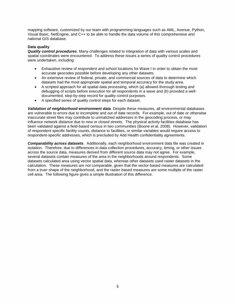
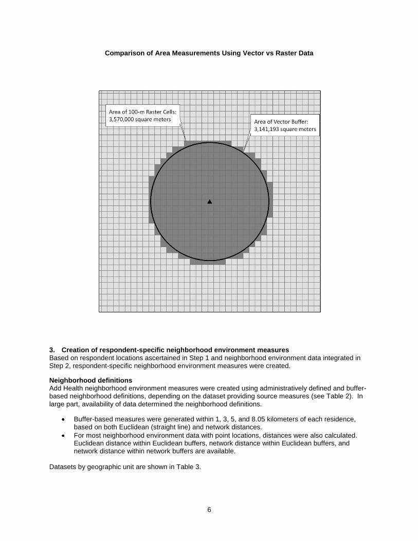
Comparability across datasets. Additionally, each neighborhood environment data file was created in isolation. Therefore, due to differences in data collection procedures, accuracy, timing, or other issues across the source data, measures derived from different source data may not agree. For example, several datasets contain measures of the area in the neighborhoods around respondents. Some datasets calculated area using vector spatial data, whereas other datasets used raster datasets in the calculation. These measures are not comparable, given that the vector-based measures are calculated from a truer shape of the neighborhood, and the raster-based measures are some multiple of the raster cell area. The following figure gives a simple illustration of this difference.

6

Comparison of Area Measurements Using Vector vs Raster Data

3. Creation of respondent-specific neighborhood environment measures Based on respondent locations ascertained in Step 1 and neighborhood environment data integrated in Step 2, respondent-specific neighborhood environment measures were created.

Neighborhood definitions Add Health neighborhood environment measures were created using administratively defined and buffer-based neighborhood definitions, depending on the dataset providing source measures (see Table 2). In large part, availability of data determined the neighborhood definitions.

Buffer-based measures were generated within 1, 3, 5, and 8.05 kilometers of each residence, based on both Euclidean (straight line) and network distances.

For most neighborhood environment data with point locations, distances were also calculated. Euclidean distance within Euclidean buffers, network distance within Euclidean buffers, and network distance within network buffers are available.

Datasets by geographic unit are shown in Table 3.

7

Neighborhood environment measures Neighborhood environment measures are contained in a series of datasets (Table 3). Refer to code book for each file for details about the source data and variables created.

Table 3. Obesity and Neighborhood Environment datasets and corresponding geographic units and filenames

NOTE: Not all files have been released as of October 2009. Dataset Geographic units Wave I filename Wave III filename

ACCRA County w1accra w3accra

Census County, tract, block group w1census w3census

Climate Nearest climate station w1climat w3climat

Coastline Nearest coastline w1coast w3coast

Street connectivity Buffers w1conn w3conn

Crime County w1crime w3crime

Employment County w1employ w3employ

Geocode type Street segment, GPS point, ZIP code, or school location (W1 only)

w1gcodes w3gcodes

Land cover Buffers w1lndcv w3lndcv

Length of day N/A (latitude) w1loday w3loday

Malls Buffer (8.05 km only) w1malls w3malls

Mobility indicator N/A (distance) -NA- w3mobind

Metropolitan Statistical Area identifier

MSA -NA- w3msa

Parks Buffers w1parks w3parks

Pollution County w1pollut w3pollut

Population counts Buffers w1pop90 w3pop00

Resources Buffers w1rcdist w3rcdist

Road type Buffers w1rtlen w3rtlen

RUCA Census tract w1ruca w3ruca

Distance to school N/A (distance) w1schdis -NA-

Mean Slope Angle Buffer (8.05 km only) w1slope w3slope

Distance to urbanized area N/A (distance) w1urbdst w3urbdst

Traffic Urbanized area w1urbtrf w3urbtrf

Weather N/A (distance to Nearest weather station)

w1weath w3weath

Web parks ZIP code w1webpark -NA-

-NA- dataset not created NOTES

Census data: To reduce potential deductive disclosure, raw census variables (raw counts) are not included in the Add Health neighborhood environment data. Instead, constructed variables (e.g., percent of persons living below the federal poverty level, percent of residents who are white non-Hispanic) were calculated for researchers.

Population density can be constructed dividing population counts by the relevant area. However, population counts are only available within Euclidean buffers, and areas within network buffers and census units are not currently available. Therefore, at this time, population density can only be calculated within Euclidean buffers (population within buffers*/straight buffer area**). *from population datasets, w1pop90 and w3pop00 **from connectivity dataset, w1conn and w3conn

The area measure in the connectivity data set is simply the area of a circle, πr². These area values are identical for all respondents, i.e., min=max=avg in all cases. The user should not need the connectivity

8

data set for this calculation because pop/ (πr²) will produce the same result. The area measures in the population data set were included expressly for the purpose of calculating population density and will also produce a more meaningful and accurate pop density value. It is therefore recommended to use the area value from the population dataset.

4. Linkage to individual-level data

Linkage of neighborhood environment variables to individual-level data was performed through complex security procedures. All spatial analyses requiring identifiable geographic locations (below the regional level) were performed in the Spatial Analysis Unit (SAU) at the Carolina Population Center at the University of North Carolina at Chapel Hill. Working with blind respondent identifiers, SAU created respondent-specific neighborhood environment measures. As part of a sanitizing procedure, these neighborhood environment measures were then cross-linked with true respondent identifiers at a third party location, which allowed the neighborhood environment measures to then be linked with individual-level Add Health interview and survey data by non-SAU Add Health personnel. Raw spatial units and locations were available only to SAU analysts, who do not have access to individual-level Add Health data.

Geographic identifiers are not available to the researchers on this project due to deductive disclosure concerns. After linking the neighborhood environmental measures to the Add Health respondent data, a comprehensive deductive disclosure review and data cleaning were performed to ensure respondent confidentiality.

Overview of each dataset

Below is a list of brief descriptions for each neighborhood environment dataset. Datasets are provided separately for Waves I and III. Full descriptions of these data can be found in the codebooks for the individual dataset. Further, the user is encouraged to find published research using data from each of the datasets below. The original data sources chosen for the Obesity and Neighborhood Environment data were selected in many cases because they have been used in the literature. The user is therefore strongly encouraged to complete literature searches in the subject area of interest to find papers that use a given dataset of interest. For example, if one is interested in census-level sociodemographic as an exposure to predict a health outcome, the author should try to search for papers in PubMed with keyword searches for “US Census”, “neighborhood poverty” and so forth. Time-varying data are provided based on residential locations at Waves I and III. ACCRA

Add Health data files: w1accra.xpt and w3accra.xpt The American Chamber of Commerce Research Association (ACCRA), now Council for Community and Economic Research [C2ER], produces the Cost of Living Index on a quarterly basis to provide a reasonably accurate measure to compare cost of living differences among urban areas. Items on which the Index is based have been carefully chosen to reflect the different categories of consumer expenditures and include housing, food, transportation, and activities for daily living. Weights assigned to relative costs are based on government survey data on expenditure patterns for midmanagement households (see C2ER website, http://www.coli.org/). All items are priced in each place at a specified time and according to standardized specifications. These Add Health datasets contain ACCRA Cost of Living Index (http://www.coli.org/) data for Waves I and III based on the respondent locations and year and quarter of Add Health interview. It is important to note that ACCRA data are not reported at a consistent geographic level. The data could only be joined to respondent locations after developing values for counties, MSAs, non-MSAs, and states using a complex algorithm. The state and county FIPS codes were then used to perform the joins.

9

In addition, ACCRA data are not reported consistently on a temporal basis. It is at the discretion of the reporting party as to the frequency.

Census Add Health data files: w1census.xpt and w3census.xpt Constructed variables in this file were created using SF3 Census data at the block group, tract, and county levels based on the location of respondents at each wave. Data are derived from the 1990 & 2000 Census CD Long Form product purchased from GeoLytics (www.geolytics.com). Respondent locations at Waves I & III were joined to Census 1990 and 2000 data geographically and temporally. Using a spatial join, the block group, tract, and county FIPS codes were assigned to each respondent for both the 1990 (Wave I) and 2000 (Wave III) census, and those FIPS codes were subsequently used to join the census variables to the respondents.

Climate

Add Health data files: w1climat.xpt and w3climat.xpt These datasets contain climate data for each Add Health Wave I and Wave III respondent based on the nearest station reporting data for each climate variable. If the climate station nearest to the respondent had no data for the variable of interest, the respondent was assigned the next station with data for the desired variable. January, July, and annual means were collected for each variable. The climate data describe the average weather over an extended period of time, in a specific region. The climate data (variables and climate station locations) were culled from the Climate Atlas of the United States, version 2.0, which brings together data from a number of climate stations for the period 1961 to 1990 and provides monthly averages for each station for that time period.

Coastline

Add Health data files: w1coast.xpt and w3coast.xpt Distance to the nearest coastline (or shoreline for any large body of water) is provided for each Wave I and Wave III respondent location. Coastline data are derived from the Data & Maps (D&M) 2004 dataset from Environmental Systems Research Institute (ESRI) in Redlands, CA (www.esri.com). The Detailed State Boundary file of D&M 2004 was used as the source data for the coastline locations.

Street Connectivity Add Health data files: w1conn.xpt and w3conn.xpt These datasets contain road network connectivity measures within 1, 3, 5, and 8.05 km (Euclidean distance) of Wave I and Wave III respondent locations. The road networks for Wave I and Wave III respondents were extracted from the StreetMap 2000 (published 1999) and StreetMap Pro (July 2003, v. 5.2) products, respectively, from Environmental Systems Research Institute (ESRI, www.esri.com) in Redlands, CA.

Crime

Add Health data files: w1crime.xpt and w3crime.xpt These datasets contain county-level crime data based on the location of Wave I and Wave III respondents. Data are based primarily on Uniform Crime Reporting (UCR) data downloaded from the National Archive of Criminal Justice Data (NACJD) Web site, which is located at http://www.icpsr.umich.edu/NACJD/. Wave I uses data primarily from 1995 (part four, “DS4: Crimes

10

Reported”, study number 6850), but imputes missing values using UCR data from 1990 and 1992-1994 in conjunction with intercensal population estimates from the Census Bureau (http://www.census.gov/popest/counties/). Wave III uses data from 2001 (DS4 study number 3721). The datasets contain crime rates per 100,000 people based on crimes reported (as opposed to arrests made), as well as some variables to help understand the quality of the crime rate data calculated for an individual. The variables used were as identical as possible to those used in the development of the crime component of the Add Health Wave I contextual database released in 1998,which contains UCR data from 1993.

Distance to School Add Health data files: w1schdis.xpt This file contains the distance between the geocoded point locations of each respondent’s Wave I location and that respondent’s school. The distance value is a Euclidean distance measure between the two points (residential location and school location) in meters.

Employment

Add Health data files: w1employ.xpt and w3employ.xpt

These datasets contain county-level employment data based on the location of Wave I and Wave III respondents. Data are based on county-level employment information from the U.S. Bureau of Labor Statistics (BLS). There are two sets of employment information in the files: (1) total county employment and unemployment counts for the years 1990-1995 (Wave I) and 2001 (Wave III), and (2) county employment counts across six industry categories. The industry categories were defined by groups of three-digit 1997 North American Industry Classification System (NAICS) codes (see employment dataset codebook). Note that there is some repetition of NAICS codes among categories.

Geocode Source

Add Health data files: w1gcodes.xpt and w3gcodes.xpt

These datasets indicate the data source of the Wave I and Wave III respondent geocodes (latitude and longitude). Street segment matches, GPS points, Zip codes, and school locations (Wave I only) were used in assigning geocodes to respondents.

Land Cover

Add Health data files: w1lndcv.xpt and w3lndcv.xpt

These Add Health datasets contain land cover metrics within 1, 3, 5, and 8.05 km (5 miles) of Wave I and Wave III respondent locations. The land cover metrics were derived from the Fragstats software package (version 3.3 build 5) using land cover data from the Multi-Resolution Land Characteristics (MRLC) Consortium. For Wave I, data were obtained from the National Land Cover Dataset for 1992 (NLCD 1992) downloaded from the U.S. Geological Survey (USGS) using the Web address http://edcwww.cr.usgs.gov/pub/data/landcover/states/. For Add Health Wave III, MRLC Consortium National Land Cover Database (NLCD 2001) files were downloaded from http://edcftp.cr.usgs.gov/pub/data/landcover/nlcd2001/superzones/landcover_zips. Six land classes are included: Water or Perennial Ice; Developed, Low and Medium Density; Developed, High Density; Developed, Recreational; Undeveloped/Natural; Agricultural.

11

Length of Day

Add Health data files: w1loday.xpt and w3loday.xpt This dataset contains the number of hours of daylight at each Wave I and Wave III respondent location based on that respondent’s latitude and survey date. Length of day (LOD) is derived from the solar declination on a given date and the terrestrial latitude of a given location. All the points at the same latitude on the same calendar date are generally considered to have the same day length. For reasons of privacy protection and potential deductive disclosure of respondent locations, only geographic latitudes between 28° north and 47° north were allowed. Any respondent locations south of 28° were assigned 28° and any respondent locations north of 47° were assigned 47°. These limits were applied to 991 respondents in Wave I and 764 respondents in Wave III and ensure that the finest degree to which a respondent location may be reverse calculated is no less than three states. For these respondents, the maximum difference between true LOD and the LOD resulting from obfuscated latitude is 38 minutes.

Mean Slope Angle Add Health data files: w1slope.xpt and w3slope.xpt These datasets contain the mean slope angle in degrees for the five-mile (radius) neighborhood around each Wave I and Wave III respondent location. Slope data were derived from elevation data obtained from the U.S. Geological Survey (USGS) Seamless Data Distribution System (SDDS, http://seamless.usgs.gov/), derived primarily from Shuttle Radar Topography Mission (SRTM) elevation data. In addition, land cover data were used in the processing to mask areas of water.

Mobility Indicator Add Health data files: w3mobind.xpt This dataset includes the distance between the respondent’s Wave I geocoded residential location and (a) the respondent’s Wave II residential location, (b) the respondent’s Wave III residential location, and (c) the respondent’s Wave I school location. The distances are straight-line measures between the point pairs and are reported in meters. Move distances less than ¼ mile (402.336 meters) were rounded down to zero and considered inconsequential and/or attributable to geocoding error. All other move distances were rounded to the nearest whole meter.

Parks Distance and Area

Add Health data files: w1parks.xpt and w3parks.xpt The public parks data for Wave I and Wave III respondents are based on the parks component of StreetMap Pro (July 2003, v. 5.2) from Environmental Systems Research Institute (ESRI) in Redlands, CA. The parks component of the StreetMap Pro dataset contains boundaries for parks, forests, and recreation areas at the national, state, and local levels. The variables include counts, counts inverse-weighted by Euclidean distance, and summary statistics of local parks by Euclidean distance buffers and Euclidean distance to each major park irrespective of distance.

12

Pollution

Add Health data files: w1pollut.xpt and w3pollut.xpt

This dataset contains county-level pollution data based on the location of Wave I and Wave III respondents. Wave I and III data are based on 1995 and 2001 (respectively) county-level emissions estimates for criteria air pollutants (CAPs) from the U.S. Environmental Protection Agency’s (EPA’s) National Emission Inventory (NEI) database. According to the EPA Web site (http://www.epa.gov/ttn/chief/net/neiwhatis.html), CAPs are “those for which EPA has set health-based standards.”

Proportional Block Group Population and Area

Add Health data files: w1pop90.xpt and w3pop00.xpt

These Wave I and III datasets contain the proportion of 1990 and 2000 (respectively) U.S. Census block group population and area (in square meters) within 1, 3, 5, and 8.05 km of each respondent. Wave I and III block group population counts were extracted from the 1990 and 2000 Census CD Long Form product (respectively) purchased from GeoLytics (www.geolytics.com).

Resource Counts and Distance (RCD) Measures

Add Health data files: w1rcdist and w3rcdist.xpt

These resource and distance datasets contain counts, counts inverse-weighted by distance, and univariate distance statistics based on Dun & Bradstreet (D&B) physical activity (PA) resources within 1, 3, 5, and 8.05 km Euclidean and network distances of Wave I (1995 D&B) and III (2001 D&B) respondent locations. Network distances were calculated for Wave I using StreetMap 2000 (published 1999) and for Wave III using StreetMap Pro (July 2003, v. 5.2). All calculations were performed according to PA categories, which were based on D&B primary Standard Industrial Classification (SIC) codes and keyword searches within the company name and trade style fields. There are a growing number of studies which examine PA resources ascertained from D&B or similar (e.g., InfoUSA) data sources. The user is encouraged to review this literature to understand how best to use these data. See also our publications on this topic (Boone et al., 2008; Gordon-Larsen et al. 2006, full references at end).

Road Type Length

Add Health data files: w1rtlen.xpt and w3rtlen.xpt

These files contain road type length data based on the location of Wave I and Wave III respondents. The road type length variables are based on the Census Feature Classification Codes (CFCCs). The roads data used for road type length calculations were extracted from StreetMap 2000 (Wave I) and StreetMap Pro (July 2003, v5.2) (Wave III) from Environmental Systems Research Institute (ESRI) in Redlands, CA (www.esri.com). The ESRI StreetMap 2000 product was derived from data developed by the company Geographic Data Technology (GDT), which has since been acquired by Tele Atlas (www.teleatlas.com). The StreetMap Pro product was derived from roads data developed by GDT, which was acquired by TeleAtlas (www.teleatlas.com).

13

RUCA

Add Health data files: w1ruca.xpt and w3ruca.xpt

This dataset contains 1990 and 2000 rural-urban commuting area (RUCA) codes at the U.S. Census tract level based on the location of Wave I and Wave III respondents. RUCA data were obtained from the U.S. department of Agriculture’s Economic Research Service and reflect the population size and direction and share of commuting patterns.

Shopping Malls Add Health data files: w1malls.xpt and w3malls.xpt Shopping mall data for the Wave I and Wave III respondent locations are derived primarily from a shopping malls dataset for publication year 1996 (calendar year 1995, with last updates in 4

th quarter

1995) and publication year 2002 (calendar year 2001, with last updates in 4th quarter 2001) purchased

from the Directory of Major Malls (DMM, www.directoryofmajormalls.com). According to the DMM web site, the DMM “has evolved in the past twenty years into a suite of data products which concentrate on the niche market of the major shopping centers and malls in the U.S. and Canada which are 250,000 square feet and above in size.”

Urbanized Area Distance

Add Health data files: w1urban.xpt and w3urban.xpt

These files contain distances to 1990 and 2000 U.S. Census Urbanized Areas (UAs) for each Wave I respondent and distances to 2000 UAs for each Wave III respondent. Distances, which were measured using respondent locations and UA boundaries projected to the Universal Transverse Mercator (UTM) coordinate system, are reported in meters. U.S. Census UAs represent boundaries for UAs with a population greater than 50,000.

Urban Traffic Congestion

Add Health data files: w1urbtrf.xpt and w3urbtrf.xpt The Texas Transportation Institute (TTI; http://tti.tamu.edu/) traffic congestion data (“Urban Mobility and Congestion Statistics”) for the TTI urban area nearest to each Wave I and Wave III respondent location are contained in these datasets. The TTI source data depict mobility and traffic congestion on freeways and major streets in 85 of the largest UAs in the United States for each year since 1982. For Wave I respondents, 1995 TTI congestion data were joined to U.S. Census 1990 Urbanized Area boundaries. For Wave III, 2001 TTI congestion data were joined to U.S. Census 2000 Urbanized Area boundaries.

Weather

Add Health data files: w1weath.xpt and w3weath.xpt

These files contain weather data for each Add Health Wave I and Wave III respondent based on the nearest weather station reporting data for the corresponding month and year of interview date. Weather describes the conditions of the atmosphere over a short period of time in a specific location. The weather source data were extracted from the National Climatic Data Center (NCDC) Dataset 3220 (DSI-3220) Summary of the Month (SOM) Cooperative (see http://www.ncdc.noaa.gov/pub/data/documentlibrary/tddoc/td3220.pdf). As the name suggests, these datasets consist of a number of meteorological variables summarized on a monthly time scale. The data

14

come primarily from the cooperative network, but also include observations from the principal meteorological stations operated by the National Weather Service.

Web Parks

Add Health data files: w1webprk.xpt This dataset is only available for Wave I and contains counts of recreational resources for the communities corresponding to the ZIP codes of Wave I respondents’ schools. The counts, which were developed via Web searches augmented by telephone calls to parks and recreation departments, were reported for a select group of recreational resources. The dataset is selective in that not all communities had data on the web or staff at parks and recreation departments willing to take calls.

15

References

Boone JE, Gordon-Larsen P, Stewart JD, et al. Validation of a GIS facilities database: quantification and implications of error. Ann Epidemiol 2008;18:371-7.

Gordon-Larsen P, Nelson MC, Page P, et al. Inequality in the built environment underlies key health disparities in physical activity and obesity. Pediatrics 2006;117:417-24.

16

Acknowledgment

This research was funded by National Institutes of Health (National Institute of Child Health and Human Development grants R01 HD39183, R01 HD041375, and K01 HD044263; National Institute of Diabetes and Digestive and Kidney Diseases grant DK56350; and National Institute on Environmental Health Sciences grant P30ES10126), National Institute of Aging NIA: K07 AG001015 and P30 AG024376; and a cooperative agreement with the Centers for Disease Control and Prevention (CDC SIP No. 5-00).

17

Appendix

Wave III Global Positioning System (GPS) reading procedure:

1. Take the GPS reading at the current residence of the respondent.

2. If the interview does not take place at the respondent’s residence collect a current residential address instead of the GPS reading.

3. If the respondent is a residential college student, in prison, or in the military and the interview takes place away from his/her usual residence collect a current address for the residential location.

4. If the respondent referred to in number 3 does not have a valid residential street address use the main street address for the facility. If this address is not known, be sure to include the full name of the facility so that an address can be obtained.

5. Good addresses do NOT contain rural routes, apartment numbers, vanity addresses, non-standard abbreviations, and misspellings.