Embed Size (px)
Citation preview
National Health and Nutrition Examination Survey:
Technical Documentation for the 1999-2004
Dual Energy X-Ray Absorptiometry (DXA) Multiple Imputation Data files
February 2008
Contents Page
1. Overview of Multiple Imputation……………………………………………………..1
2. Overview of NHANES DXA Data……………………………………………………2
2.1 DXA Examination
2.2 Missing DXA Data
3. Procedure for Multiply Imputing the NHANES DXA Data………………………….6
3.1 Sequential Regression Multivariate Imputation
3.2 Further Details of the Procedure
3.2.1 Imputation by age-gender groups
3.2.2 Variable selection
3.2.3 Transformations of the DXA variables
3.2.4 Setting lower bounds
3.3 Evaluating the Imputations
3.3.1 Evaluating the regression models
3.3.2 Evaluating the imputed values
4. Analyzing Multiply Imputed Data…………………………………………………..13
4.1 General Procedures
4.2 Combining Multiple Estimates and Standard Errors
4.3 Combining Data across NHANES Survey Cycles
4.4 Analytic Examples Using SAS-Callable SUDAAN
References…………………………………………………………………….…………….26
Tables……………………………………………………………………………………….30
Figures……………………………………………………………………………………....35
i

Analysts are strongly encouraged to read all of the following documentation. Use of the
multiply imputed data files will provide complete DXA data for all participants and more
accurate standard errors of estimates.
1. Overview of Multiple Imputation
Imputation, which refers to filling in plausible values for missing data, is a popular approach to
handling nonresponse on items in a survey for several reasons. First, imputation adjusts for
observed differences between nonrespondents and respondents. Such an adjustment is generally
not made by complete-case analysis, also known as listwise deletion, which refers to omitting cases
with incomplete data from the analysis. Second, imputation results in a completed data file, so that
the data can be analyzed using standard software packages without discarding any observed or
measured values. Third, when a data file is being produced for analysis by the public, imputation
allows the data producer to incorporate specialized knowledge about the reasons for missing data in
the imputation procedure. Moreover, the nonresponse problem is addressed in the same way for all
users, so that analyses will be consistent across users. Finally, imputation can be more effective
than reweighting in using the statistical relationships among survey variables to produce accurate
predictions of the missing data values, leading to more efficient estimates.
Single imputation, which refers to imputing just once for each missing value, does not reflect the
uncertainty stemming from the fact that the imputed values are plausible replacements for the
missing values but are not the true values themselves. As a result, analyses of singly imputed data
that treat the imputed values as if they were measured values tend to produce estimated standard
errors that are too small, confidence intervals that are too narrow, and significance tests that reject
the null hypothesis too often when it is true. For example, large-sample results reported by Rubin
and Schenker (1986) suggest that when the rate of missing information is 20% to 30%, nominal
95% confidence intervals computed from singly imputed data have actual coverage rates between
85% and 90%. Moreover, the performance of single imputation can be even worse when
inferences are desired for a multi-dimensional quantity. Large-sample results reported by Li,
Raghunathan, and Rubin (1991) demonstrate that for testing hypotheses about multi-dimensional
1
quantities, the actual rejection rate under the null hypothesis increases as the number of
components being tested increases, and the actual rate can be much larger than the nominal rate.
Multiple imputation allows the uncertainty due to imputation to be reflected in the analysis (Rubin,
1978, 1987). With multiple imputation, M > 1 plausible sets of replacements are generated for the
missing values, thereby generating M completed data files. The M sets of imputations for the
missing values are ideally independent draws from the predictive distribution of the missing values
conditional on the observed values. Each of the M completed data files is analyzed separately
using the method that would be applied if the data were complete, and the variation in results
among the M versions provides a measure of missing-data uncertainty in addition to the usual
variation due to sampling. The M sets of results may be formally combined to provide standard
errors and confidence levels that incorporate the missing-data uncertainty. Details of how to
analyze multiply imputed data are provided in Section 4. For public-use data, M is not usually
larger than 5 (to limit computational burden for analysts), which is the number of data files imputed
for the application described herein.
At the National Center for Health Statistics, multiple imputation has been applied previously to
data from the Third National Health and Nutrition Examination Survey (NHANES III: 1988-1994)
(National Center for Health Statistics, 2001), the National Health Interview Survey (Schenker et al.,
2006), and the State and Local Area Integrated Telephone Survey (Pedlow, Luke, and Blumberg,
2007).
2. Overview of NHANES DXA Data
Dual-energy x-ray absorptiometry (DXA) has long been accepted as the primary method for
measuring bone mineral content and bone mineral density because of its high precision, accuracy,
and low radiation exposure (Njeh et al., 1990; Wahner et al., 1994; WHO, 1994; Genant et al.,
1996) More recently, whole body DXA also has become one of the most widely accepted methods
of measuring body composition due to its speed, ease of use, and strong correlation with criterion
methods of assessing body composition (Lohman and Chen, 2005; Thomas et al., 2005).
2
The assessment of body composition by DXA has taken on added importance as the prevalence of
overweight and obesity in the U.S. over the past 40 years has steadily increased among both adults
and children (Flegal et al., 2002, Ogden et al., 2002). In 2003-04, 66.3% of adults 20 years of age
and older were overweight or obese and 32.2% were obese (Ogden et al., 2006). Among children
2-19 years of age, 33.6% in 2003-04 were at risk for overweight or overweight and 17.1% were
overweight (Ogden et al., 2006). Although body mass index (BMI), calculated as weight in
kilograms over height in meters squared, has been commonly used as the standard measure of
obesity in the U.S. and other countries (WHO, 1995), there are recognized limitations to the use of
BMI in assessing obesity in a population. The relationship of body fat to BMI varies with age,
gender, ethnicity, and physical conditioning (Baumgartner et al., 1995; Gallagher et al., 1996;
Deurenberg et al., 1998). Because DXA assesses the proportions of lean mass and fat mass in the
body, it is a more accurate measure of percent body fat and obesity than is BMI. In 1999, to
provide information on soft tissue composition as well as bone content, the National Health and
Nutrition Examination Survey (NHANES) implemented whole body DXA scans of survey
participants age 8 years and older. Although DXA scans of the proximal femur had been
successfully administered in the NHANES in 1988-94 to assess bone density in adults age 20 years
and over in the U.S. population (Looker et al., 1998), these scans were not included in the 1999
2004 protocol.
2.1 DXA Examination
In each NHANES survey year, a nationally representative sample of the U.S. civilian non-
institutionalized population is selected using a complex, stratified, multistage probability sampling
design. Approximately 5,300 individuals of all ages are interviewed in their homes yearly; of
these, approximately 5,000 complete the health examination component of the survey. The 1999
2004 NHANES includes an oversampling of non-Hispanic blacks, Mexican Americans, low-
income whites, adolescents 12-19 years of age, and persons 60 years of age and over to provide
more reliable estimates for these groups. Although a nationally representative sample of the U.S. is
selected each survey year, the NHANES data are released as public use data in two-year cycles to
provide adequate sample sizes for subgroup analyses.
DXA scans were administered to eligible survey participants 8 years of age and older in the
NHANES mobile examination centers (MECs). Females of ages 12-59 years and menstruating 8
3
11 year olds were permitted to take the DXA examination only if a pregnancy test taken at the time
of the exam was negative. Females also were excluded from the examination if they said they were
pregnant at the time of the exam, even if the pregnancy test was negative. Individuals were
excluded from the DXA examination who reported taking tests with radiographic contrast material
in the past 72 hours, participated in nuclear medicine studies in the past 3 days, or had a self-
reported weight (> 300 pounds) or height (> 6’5”) over the DXA table limit. All other participants
were asked to have a DXA scan taken.
The whole body DXA scans were acquired using a Hologic QDR 4500A fan-beam densitometer
(Hologic, Inc., Bedford, Massachusetts) following the manufacturer’s acquisition procedures.
Hologic DOS software version 8.26:a3* was used to acquire all scans; scanning was done in the
fast mode. Participants wore disposable paper gowns and were asked to remove all objects that
would interfere with obtaining an analyzable scan image, such as jewelry, watches, hair ornaments,
glasses, keys, and wallets. The DXA examination protocol is documented in the January 2004
Body Composition Procedures Manual on the NHANES website
http://www.cdc.gov/nchs/nhanes.htm.
The scan for each survey participant was reviewed and analyzed by the University of California,
San Francisco (UCSF), Department of Radiology using standard radiologic techniques and study-
specific protocols developed for the NHANES. Hologic Discovery software, version 12.1, was
used to analyze the scans. Soft tissue measures: fat mass (gm), lean mass including bone mineral
content (gm), lean mass excluding bone mineral content (gm), and percent (%) body fat and bone
measures: bone mineral content (BMC) (gm), bone area (cm2), and bone mineral density (BMD)
(gm/cm2) were obtained for the head, arms, legs, and trunk. Bone measures also were obtained for
the pelvis, ribs, thoracic spine, and lumbar spine. Invalidity codes were applied by the UCSF to the
entire scan or to body regions that could not be analyzed accurately. Data were coded as invalid as
a result of jewelry and other objects not removed by participants; the presence of non-removable
objects such as prostheses, pacemakers, implants, casts, etc.; excessive x-ray “noise” due to obesity
(applied to the trunk region only); arm/leg overlap; body parts out of the DXA table scan area;
positioning problems (head, arms/hands or feet turned); and other reasons, which included
participant motion, missing limbs, and unknown artifacts. Such invalid data were set to missing in
the data file. If data for any region were missing, total body values such as total mass and total %
4
body fat were coded as missing also since regional data were summed to equal total values.
Additional information on the DXA data collection and quality control review procedures,
adjustments made to the DXA data, and the structure of the DXA release data files can be found in
the DXA Data Documentation on the NHANES website.
Of the 21,230 eligible DXA participants aged 8 years and over who participated in the MEC
examinations in 1999-2004, scans with 100% non-missing data were obtained from 16,973 or
80.0%. (For this calculation, pregnant women were not counted as eligible participants.)
2.2 Missing DXA Data
The percentages of survey participants in 1999-2004 with data missing for one or more regions are
provided in Table 1 by gender-age group and in Table 2 by BMI category. The percentages
increase with increasing age and BMI. Because DXA data missingness is related to age, BMI,
weight and height (due to the weight and height exclusions mentioned in Section 2.1), and possibly
other characteristics, participants with missing data cannot be treated as a random subset of the
original sample. Otherwise, analytic results may be biased toward participants with the least
amount of missing data.
To resolve the problem of potential biases due to missing DXA data, multiple imputation of the
missing data was performed for the survey years 1999-2004. Five completed data files containing
both the non-missing and imputed DXA data values were created to allow the assessment of
variability due to imputation. For the missing data, each of the 5 data files contains a different set
of imputed values, whereas for the non-missing data, the values are identical across the 5 files
(since no imputation was carried out for them). The files include DXA total body values, subtotal
values (excludes head values), and regional values for fat mass, % body fat, lean mass including
bone mineral content, lean mass excluding bone mineral content, BMC, bone area, and BMD;
variables indicating the DXA values that were imputed; and variables indicating the reason for
invalid regional values. In addition, the common sequence identification number (SEQN) for each
participant is provided for purposes of merging the multiply imputed DXA data with other
NHANES data. DXA data are not provided for pregnant women and participants with amputations
other than fingers or toes. The DXA data have been released in two-year cycles: 1999-2000, 2001
5
2002, and 2003-2004. For computational convenience, the five completed data files have been
concatenated into a single file for each release cycle.
3. Procedure for Multiply Imputing the NHANES DXA Data
The type of imputation procedure used for the NHANES DXA data is described in Section 3.1.
This is followed by discussions of some further details of the models used (Section 3.2) and
evaluations of the models and imputations (Section 3.3). Although the discussions of the model
development and evaluations are presented sequentially, they were actually performed in an
iterative fashion, because a chosen model leads to a specific set of evaluation results, which then
suggests modifications to the model, and so on.
3.1 Sequential Regression Multivariate Imputation
The multiple imputations for the NHANES DXA data were created using sequential regression
multivariate imputation (SRMI) (Raghunathan et al., 2001), as implemented by the module
IMPUTE in IVEware (Raghunathan et al., 2002), a SAS-callable software package for imputation
and variance estimation developed by the Survey Methodology Program at the University of
Michigan’s Institute for Social Research. IVEware is available at the website
http://www.isr.umich.edu/src/smp/ive.
A brief description of SRMI is as follows; see Raghunathan et al. (2001) for further details. Let X
denote the fully-observed variables, and let Y1 ,Y2 ,...,Yk denote k variables with missing values,
ordered by the amount of missingness, from least to most. The imputation process for Y1 ,Y2 ,...,Yk
proceeds in c iterations. In the first iteration: the regression of Y1 on X is fitted to the cases with
Y1 observed, and the missing values of Y1 are imputed (randomly from an approximate predictive
distribution based on the fitted regression); then the regression of Y2 on X and Y1 (including the
imputed values of Y1 ) is fitted to the cases with Y2 observed, and the missing values of Y2 are
imputed; then the regression of Y3 on X , Y1 , and Y2 is fitted to the cases with Y3 observed, and the
missing values of Y3 are imputed; and so on, until the regression of Yk on X ,Y1 ,Y2 ,...,Yk −1 is fitted
to the cases with Yk observed, and the missing values of Yk are imputed.
6
In iterations 2 through c , the imputation process carried out in iteration 1 is repeated, except that
now, in each regression, all variables except for the variable to be imputed are used as predictors
(with their most recent imputed values included). Thus: the regression of Y1 on X ,Y2 ,Y3 ,...,Yk is
fitted to the cases with Y1 observed, and the missing values of Y1 are re-imputed; then the
regression of Y2 on X ,Y1 ,Y3 ,...,Yk is fitted to the cases with Y2 observed, and the missing values of
Y2 are re-imputed; and so on. After c iterations, the final imputations of the missing values in
Y1 ,Y2 ,...,Yk are used.
For each regression in the SRMI procedure, IVEware allows the use of a normal linear regression
model if the outcome variable is continuous, a logistic regression model if the outcome variable is
binary, a multinomial logit model if the outcome variable is categorical with more than two
categories, a Poisson regression model if the outcome variable is a count, and a two-stage model if
the outcome variable is semi-continuous. In addition, IVEware allows bounds to be placed on the
variables being imputed, by drawing the imputed values from truncated predictive distributions;
and it allows for restrictions to be placed on one variable based on the value of another variable, as
might be needed to account for skip patterns in a survey. The features of IVEware were
particularly helpful in the context of multiply imputing NHANES DXA data, because missing data
on both continuous and categorical (non-DXA) variables were handled during the imputation
process (see Section 3.2.2), and bounds were placed on the imputed values for the DXA variables
(see Section 3.2.4).
By including every variable other than the variable being imputed as predictors in each regression
model, and by cycling through the various regression models, SRMI builds in relationships among
the variables included in the imputation procedure. This was especially important in the context of
the NHANES DXA data, because the DXA variables are highly interrelated.
Because SRMI requires only the specification of individual regression models for each of the Y
variables, it does not necessarily imply a joint model for all of the Y -variables conditional on X .
(See Raghunathan et al., 2001 and Van Buuren et al., 2006 for further discussion of this point.)
However, the flexibility of the procedure regarding various types of variables as well as placing
bounds on the variables being imputed allowed it to handle complicating factors in the NHANES
7
DXA imputation project that would have been very difficult to handle using a method based on a
full joint model. Moreover, had the variables all been continuous, and had no bounds been placed
on the imputations, the SRMI-based imputation procedure would actually have been equivalent to
imputation based on a multivariate normal model.
The idea of imputing variables sequentially using regression models dates back at least to
Kennickell (1991), who used such an algorithm for multiply imputing missing values for the
Survey of Consumer Finances of the Federal Reserve Board. Another software package for
multiple imputation based on this idea is MICE (multiple imputation by chained equations) (Van
Buuren and Oudshoorn, 1999), which has a stand-alone version as well as versions for R and S-
Plus (see http://www.multiple-imputation.com). In addition, the idea has been implemented in a
module for Stata; see Roylston (2005).
3.2 Further Details of the Procedure
3.2.1 Imputation by age-gender groups
The DXA data were categorized by 10 gender-age groups for the imputation procedure: males 8
11 years, males 12-19 years, males 20-39 years, males 40-59 year, males 60+ years, females 8-11
years, females 12-19 years, females 20-39 years, females 40-59 years, and females 60+ years. The
SRMI procedure was implemented separately within each of the groups. Ten iterations of the
procedure were used to create one completed dataset. To create multiple imputations (i.e., 5
completed data files), the procedure was repeated independently 5 times. After imputation, the data
for the gender-age groups were concatenated.
3.2.2 Variable selection
When multiple imputations are being created, it is beneficial to include a large number of predictors
in the imputation model, especially variables that are considered predictive of the items being
imputed and variables that will be used in subsequent analyses of the multiply imputed data (Meng,
1994; Rubin, 1996; Little and Raghunathan, 1997). In the context of a survey with complex sample
design, the predictors should also include variables related to the design. Based on these
considerations, a large number of variables were included in the imputation models for the
NHANES DXA data in addition to the DXA variables themselves, including demographic,
socioeconomic, and geographic variables, body measurements, indicators of health, variables on
8
diet and use of medications, blood test results, and variables related to the design of the NHANES
sample. Complete lists of the DXA and non-DXA variables in the models are given in Tables 3
and 4, respectively. In addition to the missingness on the DXA variables, some of the non-DXA
variables had missing values as well. The missing values for the non-DXA variables were imputed
as part of the SRMI procedure, but these imputed values were not included in the release of the
multiply imputed DXA data.
If related non-DXA variables were found to be nearly linearly dependent, so that the stability of the
SRMI procedure was affected, only one of the variables was chosen for inclusion in the model.
Collinearity was judged not to be a problem for BMI, weight, height, waist circumference, and
waist circumference/height, and all were included in the model. Body mass index was included as
both a continuous variable and as a categorical variable since both are used in the analysis of DXA
data. Although not released publicly to protect the confidentiality of survey participants, the
variables METRO and REGION were included in the model to account for clustering in the
complex sample design. A categorical variable (SDDSRVYR) for the survey cycles (1999-2000,
2001-2002, 2003-2004) was included to account for possible changes over time.
If the cells for a categorical variable were sparse, the value of the variable in prediction was
evaluated. If sparse data resulted in failure of the algorithm to converge and did not aid in
prediction, the variable was dropped from the model. Moreover, some categorical variables that
were considered important predictors were included with their categories collapsed to handle sparse
data (e.g., general health condition, alcohol consumption, and BMI). Particular attention was paid
to variables that not only had sparse cells, but also considerable missing data.
3.2.3 Transformations of the DXA variables
The linear regression models for the DXA variables in the SRMI procedure assume normal
distributions for the error terms in the regression equations. To make this assumption more tenable,
transformations were used for the DXA variables in the imputation procedure. After multiple
imputations were created on the transformed scale, the imputed values for the DXA variables were
back-transformed to their original scales.
9
Several alternative approaches to transformation of the DXA variables were explored, including no
transformation, logarithmic transformation, and an iterative Box-Cox power transformation method
(Box and Cox, 1964). When modeling was performed using the untransformed DXA variables, the
imputation procedure tended to produce physiologically implausible minimum values. When the
logarithmic transformation was used for all of the DXA variables, the imputation procedure
appeared to over-predict values at the upper ends of the distributions. After additional exploration
of alternatives for transformation of the DXA data, the iterative Box-Cox method was selected.
The iterative Box-Cox algorithm started with initial estimates of 1 for the exponents of the power
transformations for all of the DXA variables. The algorithm then iteratively cycled through the
variables one by one, updating their estimated transformations. Within each iteration, the cycling
and updating proceeded as follows. First, the DXA variables were randomly ordered in a sequence.
Then, for each variable in the sequence, the linear regression model that would be used to impute
missing values of that variable in the SRMI procedure was fitted to the complete cases, with the
transformations of all of the other variables fixed at their most recent estimates, and the method of
Box and Cox (1964) was used to obtain a new estimate of the optimal transformation for the
variable in question. The power transformation for that variable was then updated to the new
estimate, and the algorithm moved on to the next variable in the sequence, and so on, until all of the
transformations were updated. The iterations continued until the set of estimated transformations
converged. The iterative Box-Cox algorithm was implemented separately within each of the 10
gender-age groups used for imputation, and the exponents for the power transformations of the
DXA variables determined by the algorithm ranged from -0.50 to 2.50.
3.2.4 Setting lower bounds
Even after the transformations of the DXA variables in the imputation model were determined,
evaluations of the imputations indicated occasional instances of imputed values that were
implausibly low. This issue was resolved by placing lower bounds on the imputed values, as
allowed by IVEware (see Section 3.1). Within each of the gender-age groups used for imputation,
the lower bound for each DXA variable (before transformation) was set at the minimum of the non-
missing values divided by 2 . The minimum observed value divided by 2 is also used with the
NHANES laboratory data to calculate “fill” values below the level of detection (LOD).
10
3.3 Evaluating the Imputation Procedure
Evaluations of the imputation procedure were carried out in terms of both the regression models for
the DXA variables and the imputed values themselves.
3.3.1 Evaluating the regression models
Plots of the residuals from fitting the regression models used to impute the DXA variables in the
SRMI procedure to the complete cases were examined, with emphasis on plots of the residuals
versus the fitted values and normal probability plots. In general, the plots indicated good fits of the
regression models, little evidence of heteroscedasticity (i.e., non-constant error variances), and
nearly normal error distributions. However, plots of the residuals versus the fitted values for some
of the head measurement variables displayed “fan shapes,” indicating possible heteroscedasticity.
The estimated Box-Cox transformations for these variables (see Section 3.2.3) tended to be quite
strong as well. Re-fitting the regression models with untransformed or logarithm-transformed head
variables did not improve the fanning in the plots, so the decision was made to continue using the
estimated transformations. It was also thought that, while heteroscedasticity could result in
implausibly low imputed values, the lower bounds described in Section 3.2.4 would counteract this
effect.
Influential observations in the regression models were identified from plots of the residuals and
from review of the numerical diagnotic DFFITS (Belsley et al., 1980). Sensitivity of the
imputations to removal of the influential observations was examined by re-implementing the
imputation procedure with the influential observations removed. If lower bounds were not
imposed on the imputations (see Section 3.2.4), removal of the influential observations
occasionally decreased the prevalence of implausibly low values for some variables but increased
the prevalence for other variables. Removal of the influential observations also occasionally
lowered what were considered to be reasonably high imputed values for still other variables. For
most variables, however, removal of the influential observations made little difference in the
imputation of the DXA variables. Therefore, the influential observations were retained in the
imputation procedure, with the setting of lower bounds resolving the issue of implausibly low
imputed values, as discussed earlier (Section 3.2.4).
11
3.3.2 Evaluating the imputed values
To assess whether the imputed DXA values might have disproportionately high survey weights and
thus be overly influential, the distributions of the survey weights for the non-missing and imputed
values were compared. No systematic relations were found between the survey weights and the
occurrence of missing values.
The imputed values were examined in several different ways, by gender-age group, to assess
whether they appeared reasonable. For example, total DXA mass, calculated as the sum of the
imputed DXA regions, should be highly correlated with measured body weight from the NHANES
physical examination, if the imputation is accurate. This was found to be the case for all 10 gender-
age groups, based on review of plots of total DXA mass versus measured body weight, with
separate plotting symbols used for participants with no missing DXA data and participants with
varying amounts of imputed data; see, for example, Figure 1.
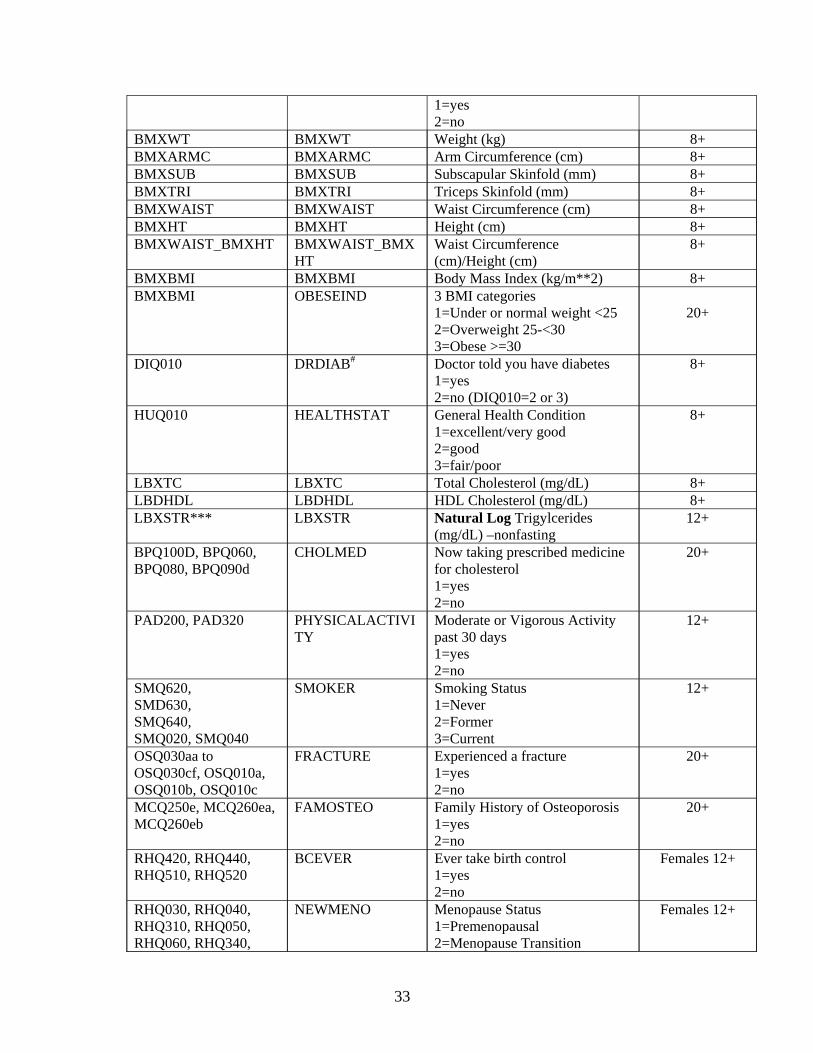
Plots of DXA total fat or truncal fat versus variables such as measured BMI, body weight, waist
circumference, and waist circumference divided by height were created; see, for example, Figures 2
and 3. The plots showed that the relations involving the imputed DXA values were similar to those
involving the non-missing DXA values. The plots also reflected the fact that imputed values for
participants with body weight greater than 300 pounds (who were not scanned) and imputed truncal
fat values for participants with missing data due to obesity “noise” were extrapolated beyond the
observed values, as would be expected.
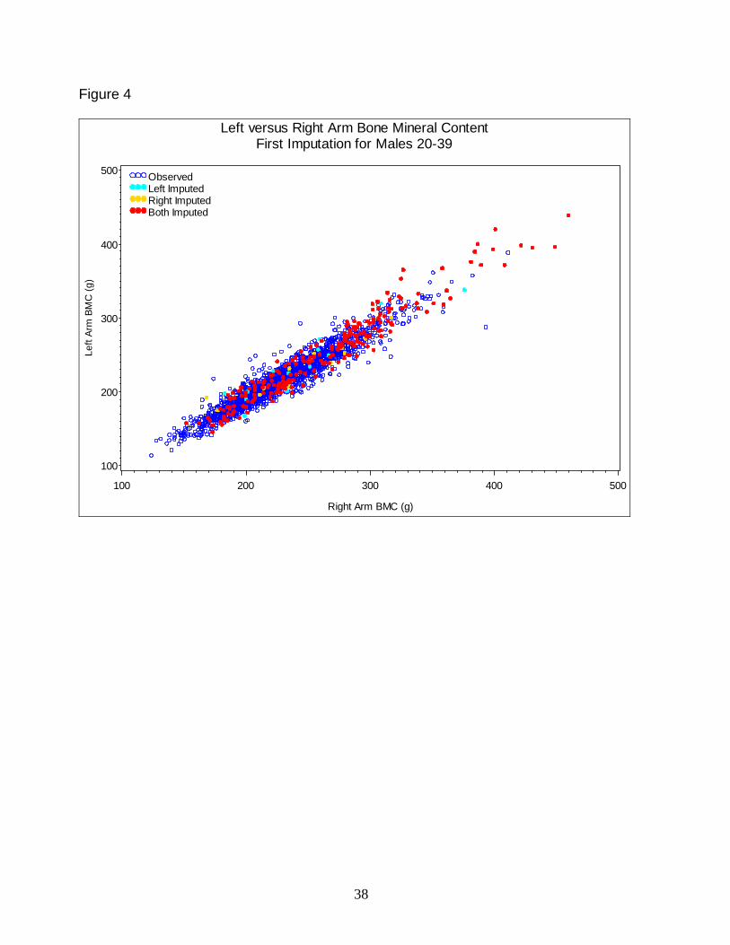
Plots of DXA values for left limbs and ribs versus right limbs and ribs were also examined; see, for
example, Figure 4. Again, the relations involving the imputed data values were similar to those
involving the non-missing data values. Moreover, the association between left and right limb
values was generally strong for both imputed and non-missing data. However, the association
between values for the left and right ribs tended to be weak for both the imputed and the non-
missing data, and users should take note of this finding.
As a final example of comparing imputed and non-missing DXA values, numerical summaries
were compared; see, for example, Figure 5, which illustrates the comparison for the left arm area
(DXDLAA). Such comparisons tended to produce plausible results, especially in light of the fact
12
that participants with missing DXA values were known to often have different characteristics from
participants with non-missing values. For example, large maximum imputed values were found to
belong to participants with high observed BMIs and were judged to be reasonable. Similarly, a few
very small imputed values seen across all five data files were found to belong to participants with
low observed BMIs and also were judged to be reasonable.
Since multiple imputation of a variable is supposed to reflect uncertainty due to missing data, some
variability among the 5 imputed values for a participant is to be expected. For some participants,
however, imputed values for DXA variables were found to vary extremely (from very low values to
very high values) among the 5 imputations. Reviews of the data for such participants showed that
the values of all of their DXA variables, as well as their measured height and weight (important
predictor variables in the imputation models) were missing and therefore had been imputed.
Because of these special circumstances and the extreme variability of the imputed values, the DXA
data for these participants have been placed in separate files (see the DXA Data File
Documentation on the NHANES website). Analysts should be aware of the highly variable nature
of these imputed DXA data when considering the use of these separate files.
4. Analyzing Multiply Imputed Data
4.1 General Procedures
Analyzing a multiply imputed dataset is similar to analyzing a conventional dataset with no missing
values. Most statistical analysis procedures that would be appropriate for other NHANES data will
be appropriate for use with the multiply imputed DXA data. The only major difference is that any
estimation procedure must be carried out 5 times, once for each version of the completed data.
Because of the complex survey design used in NHANES, traditional methods of statistical analysis
based on the assumption of a simple random sample may not be reliable. Sample weights are
needed to produce correct estimates of population quantities. Other aspects of the sample design
(e.g. PSU pairings) should be taken into account to obtain correct standard errors and significance
levels for hypothesis tests. Use of computer software for data from complex samples, such as
SUDAAN, STATA, or IVEware is strongly recommended. Appropriate methods for the analysis
13
of NHANES data are described in the NHANES Analytic and Reporting Guidelines on the
NHANES website http://www.cdc.gov/nchs/nhanes.htm.
Users of the NHANES multiply imputed DXA data files should, for the most part, follow the
guidelines given for analysis of the other NHANES public-use files. To merge the multiply
imputed DXA data with data from other NHANES 1999-2004 public-use files, the common
sequence identification number variable (SEQN) should be used.
4.2 Combining Multiple Estimates and Standard Errors
When producing statistical estimates from the multiply imputed DXA data files, the same
estimation procedure should be applied to each of the 5 versions of the completed data. The 5 sets
of results may then be combined to produce a single statistical summary that formally incorporates
uncertainty due to missing data into standard errors, significance levels, etc. In this section,
methods for combining the multiple sets of results are described for the common case in which a
scalar (one-dimensional) quantity is being estimated; see Rubin and Schenker (1986), Rubin
(1987), and Barnard and Rubin (1999) for further details and derivations. (Multiple-imputation
methods for significance tests involving multi-dimensional quantities are discussed in Rubin, 1987,
Li, Meng, Raghunthan, and Rubin, 1991, Li, Raghunathan, and Rubin, 1991, and Meng and Rubin,
1992.)
Suppose that one is interested in producing an estimate and confidence interval for a population
quantity Q, which may be a prevalence rate, mean, median, regression coefficient, etc. One must
first calculate an estimate and standard error for Q from each of the M completed datasets, using
methods that would be statistically appropriate if the data had no missing values. As mentioned in
Section 4.1, because the 1999-2004 NHANES employed a complex sample design, one should use
ˆ ˆ ˆQ Q2methods appropriate for complex samples. Let 1, ,..., QM denote the M estimates of Q, and let
ˆ ˆ ˆV V, ,..., V denote the associated variance estimates (squared standard errors) from the analyses of 1 2 M
the M completed datasets. The combined estimate of Q is simply the mean of the M individual M
estimates, Q = ∑ ˆ l / . The combined standard error for this estimate is based on the following Q M l=1
two quantities:
14
• The within-imputation variance, which is the mean of the M individual variance estimates, M
that is, W = ∑ ˆ l /V M . l=1
• The between-imputation variance, which is the sample variance of the M individual M
2estimates of Q, that is, B = ∑(Q Qˆ l − ) /( M −1) .
l=1
The total variance combines the within- and between-imputation variances as follows:
M +1T W + B T , is the combined standard error = . The square root of this total variance,M
associated with the combined estimate Q .
In many cases, an acceptable 95% confidence interval for Q can be formed based on an
approximate normal distribution: Q ±1.96 T (where 1.96 is the 97.5th percentile of the standard
normal distribution). A more accurate approximation, derived by Rubin and Schenker (1986),
replaces the multiplier 1.96 with the 97.5th percentile of Student's t-distribution with degrees of
⎡ ⎛ M ⎞⎛ W ⎞⎤2
freedom given by ν = (M −1) 1 + ⎜ .RS ⎢ ⎟⎜ ⎟⎥⎣ ⎝ M +1⎠⎝ B ⎠⎦
The Rubin/Schenker approximation is based on the assumption that if the data were complete, the
analysis of the dataset would be based on a normal distribution or a t-distribution with large degrees
of freedom. Barnard and Rubin (1999) relaxed this assumption to allow for the possibility of small
complete-data degrees of freedom, and derived the following degrees of freedom to replace the
⎛ ⎞−1
1 1Rubin/Schenker formula in the multiple-imputation analysis: ν BR = ⎜ + ⎟ , whereν k⎝ RS ⎠
( + 1) d d Wk = and d denotes the complete-data degrees of freedom. (Note that d also represents(d + 3) T
the degrees of freedom for the analysis of each of the M completed datasets.)
ˆ ˆ ˆ ˆ ˆ ˆOnce the estimates Q Q, ,..., Q and V V, ,..., V have been obtained by analyzing each of the M1 2 M 1 2 M
completed datasets, it is relatively straightforward to implement the combining rules outlined in this
15
section by using a spreadsheet program, a macro, a specially written program, or even just a
calculator. However, the increasing availability of software packages that analyze the completed
datasets and implement the combining rules is helping to facilitate multiple-imputation analyses.
For example, the SAS-callable package IVEware that was used to create the NHANES DXA
multiple imputations (see Section 3.1) has three modules for performing various multiple-
imputation analyses incorporating complex sample designs. SAS-callable SUDAAN performs
such analyses as well, and two examples of its use are given in Section 4.4.
4.3 Combining Data across NHANES Survey Cycles
The DXA data files are being released to correspond to the original NHANES data release cycle.
One data file is released for each cycle: 1999-2000, 2001-2002, and 2003-2004. Each of these data
files contains 5 completed datasets organized as 5 records per survey participant. If a data item was
missing, then the imputed values are used and these data items will not be the same across the 5
records per person. Examples of how to use each data cycle, with 5 records per person, are shown
in section 4.4 below.
It should be noted that combining data from more than one two-year data cycle is
recommended to increase the sample size and to produce statistically reliable estimates. If more
than one data cycle is to be combined to create a 4 year or six year data file, then the multiply
imputed data files for each cycle can simply be concatenated. That is, a data file for 1999-2004 can
be formed by simply concatenating the three individual files for 1999-2000, 2001-2002, and 2003
2004. The resulting data file will still have 5 records per person and analysis as described in
section 4.2 can proceed. One important analytic aspect of such combined data files is that the
sample weights will need to be adjusted if annualized estimates are required. General information
on the statistical analysis of combined 4 or 6 year data files, including the adjustment of sample
weights, are described in the NHANES Analytic and Reporting Guidelines on the NHANES
website http://www.cdc.gov/nchs/nhanes.htm
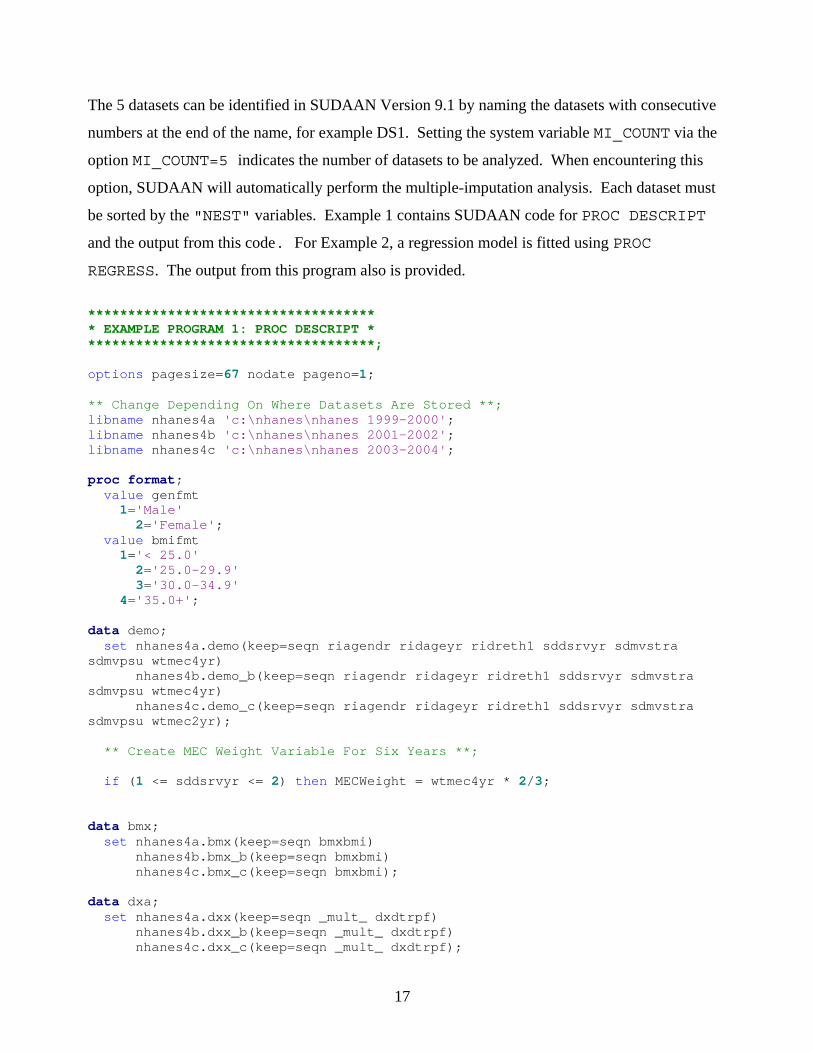
4.4 Analytic Examples Using SAS-Callable SUDAAN
SAS-callable SUDAAN is a versatile software package for analyzing data from complex surveys.
This section provides code for two examples for analysis of the NHANES multiply imputed DXA
data using SUDAAN Version 9.1, which includes a built-in option for analyzing multiply imputed
data. The code in the examples has to be modified for a user’s particular analysis.
16
The 5 datasets can be identified in SUDAAN Version 9.1 by naming the datasets with consecutive
numbers at the end of the name, for example DS1. Setting the system variable MI_COUNT via the
option MI_COUNT=5 indicates the number of datasets to be analyzed. When encountering this
option, SUDAAN will automatically perform the multiple-imputation analysis. Each dataset must
be sorted by the "NEST" variables. Example 1 contains SUDAAN code for PROC DESCRIPT
and the output from this code. For Example 2, a regression model is fitted using PROC
REGRESS. The output from this program also is provided.
************************************ * EXAMPLE PROGRAM 1: PROC DESCRIPT * ************************************;
options pagesize=67 nodate pageno=1;
** Change Depending On Where Datasets Are Stored **;libname nhanes4a 'c:\nhanes\nhanes 1999-2000';libname nhanes4b 'c:\nhanes\nhanes 2001-2002';libname nhanes4c 'c:\nhanes\nhanes 2003-2004';
proc format;value genfmt1='Male' 2='Female';
value bmifmt 1='< 25.0' 2='25.0-29.9' 3='30.0-34.9'
4='35.0+';
data demo; set nhanes4a.demo(keep=seqn riagendr ridageyr ridreth1 sddsrvyr sdmvstra
sdmvpsu wtmec4yr)nhanes4b.demo_b(keep=seqn riagendr ridageyr ridreth1 sddsrvyr sdmvstra
sdmvpsu wtmec4yr)nhanes4c.demo_c(keep=seqn riagendr ridageyr ridreth1 sddsrvyr sdmvstra
sdmvpsu wtmec2yr);
** Create MEC Weight Variable For Six Years **;
if (1 <= sddsrvyr <= 2) then MECWeight = wtmec4yr * 2/3;else MECWeight = wtmec2yr * 1/3;
data bmx; set nhanes4a.bmx(keep=seqn bmxbmi)
nhanes4b.bmx_b(keep=seqn bmxbmi)nhanes4c.bmx_c(keep=seqn bmxbmi);
data dxa; set nhanes4a.dxx(keep=seqn _mult_ dxdtrpf)
nhanes4b.dxx_b(keep=seqn _mult_ dxdtrpf)nhanes4c.dxx_c(keep=seqn _mult_ dxdtrpf);
17

data ds1 ds2 ds3 ds4 ds5; merge demo bmx dxa;by seqn;select(_mult_);when(1) output ds1;when(2) output ds2;when(3) output ds3;when(4) output ds4;when(5) output ds5;otherwise;
end;
%macro Sort;%do i = 1 %to 5;proc sort data=ds&i;by sdmvstra sdmvpsu;
run;%end;%mend Sort;%Sort;
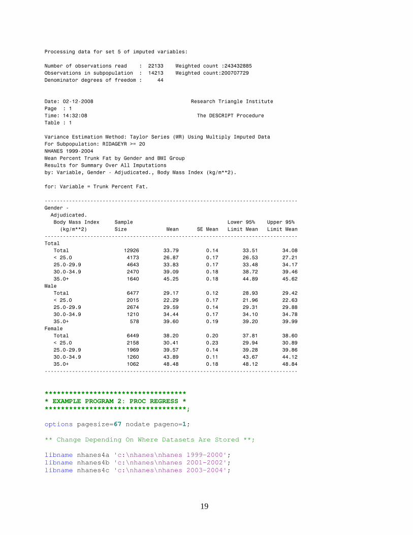
proc descript data=ds1 mi_count=5 design=wr;nest sdmvstra sdmvpsu;weight MECWeight;
** Select If 20+ **;
subpopn ridageyr >= 20;subgroup riagendr bmxbmi;recode bmxbmi=(0 25 30 35);levels 2 4; var dxdtrpf;table riagendr*bmxbmi;print nsum mean semean lowmean upmean/style=nchs;
rformat riagendr genfmt.;rformat bmxbmi bmifmt.;rtitle "NHANES 1999-2004";rtitle "Mean Percent Trunk Fat by Gender and BMI Group";
****************************************************** * SUDAAN OUTPUT FOR EXAMPLE PROGRAM 1: PROC DESCRIPT * ******************************************************;
Processing data for set 1 of imputed variables:
Number of observations read : 22133 Weighted count :243432885 Observations in subpopulation : 14213 Weighted count:200707729 Denominator degrees of freedom : 44
.
.
.
18
-----------------------------------------------------------------------------------
-----------------------------------------------------------------------------------
Processing data for set 5 of imputed variables:
Number of observations read : 22133 Weighted count :243432885 Observations in subpopulation : 14213 Weighted count:200707729 Denominator degrees of freedom : 44
Date: 02-12-2008 Research Triangle Institute Page : 1 Time: 14:32:08 The DESCRIPT Procedure Table : 1
Variance Estimation Method: Taylor Series (WR) Using Multiply Imputed Data For Subpopulation: RIDAGEYR >= 20 NHANES 1999-2004 Mean Percent Trunk Fat by Gender and BMI Group Results for Summary Over All Imputations by: Variable, Gender - Adjudicated., Body Mass Index (kg/m**2).
for: Variable = Trunk Percent Fat.
Gender - Adjudicated. Body Mass Index Sample Lower 95% Upper 95%
(kg/m**2) ---------------------
Size --------------
Mean------------
SE Mean------------
Limit Mean-------------
Limit Mean -----------
Total Total 12926 33.79 0.14 33.51 34.08 < 25.0 4173 26.87 0.17 26.53 27.21 25.0-29.9 4643 33.83 0.17 33.48 34.17 30.0-34.9 2470 39.09 0.18 38.72 39.46 35.0+ 1640 45.25 0.18 44.89 45.62 Male Total 6477 29.17 0.12 28.93 29.42 < 25.0 2015 22.29 0.17 21.96 22.63 25.0-29.9 2674 29.59 0.14 29.31 29.88 30.0-34.9 1210 34.44 0.17 34.10 34.78 35.0+ 578 39.60 0.19 39.20 39.99 Female Total 6449 38.20 0.20 37.81 38.60 < 25.0 2158 30.41 0.23 29.94 30.89 25.0-29.9 1969 39.57 0.14 39.28 39.86 30.0-34.9 1260 43.89 0.11 43.67 44.12 35.0+ 1062 48.48 0.18 48.12 48.84
*********************************** * EXAMPLE PROGRAM 2: PROC REGRESS * ***********************************;
options pagesize=67 nodate pageno=1;
** Change Depending On Where Datasets Are Stored **;
libname nhanes4a 'c:\nhanes\nhanes 1999-2000';libname nhanes4b 'c:\nhanes\nhanes 2001-2002';libname nhanes4c 'c:\nhanes\nhanes 2003-2004';
19

proc format;value genfmt1='Male' 2='Female';
value bmifmt 1='< 25.0' 2='25.0-29.9' 3='30.0-34.9'
4='35.0+';
data demo; set nhanes4a.demo(keep=seqn riagendr ridageyr ridreth1 sddsrvyr sdmvstra
sdmvpsu wtmec4yr)nhanes4b.demo_b(keep=seqn riagendr ridageyr ridreth1 sddsrvyr sdmvstra
sdmvpsu wtmec4yr)nhanes4c.demo_c(keep=seqn riagendr ridageyr ridreth1 sddsrvyr sdmvstra
sdmvpsu wtmec2yr);
** Create MEC Weight Variable For Six Years **;
if (1 <= sddsrvyr <= 2) then MECWeight = wtmec4yr * 2/3;else MECWeight = wtmec2yr * 1/3;
data bmx; set nhanes4a.bmx(keep=seqn bmxbmi)
nhanes4b.bmx_b(keep=seqn bmxbmi)nhanes4c.bmx_c(keep=seqn bmxbmi);
data dxa; set nhanes4a.dxx(keep=seqn _mult_ dxdtrpf)
nhanes4b.dxx_b(keep=seqn _mult_ dxdtrpf)nhanes4c.dxx_c(keep=seqn _mult_ dxdtrpf);
data ds1 ds2 ds3 ds4 ds5; merge demo bmx dxa;by seqn;select(_mult_);when(1) output ds1;when(2) output ds2;when(3) output ds3;when(4) output ds4;when(5) output ds5;otherwise;
end;
%macro Sort;%do i = 1 %to 5;proc sort data=ds&i;by sdmvstra sdmvpsu;
run;%end;%mend Sort;%Sort;
proc regress data=ds1 mi_count=5 design=wr;nest sdmvstra sdmvpsu;weight MECWeight;
20
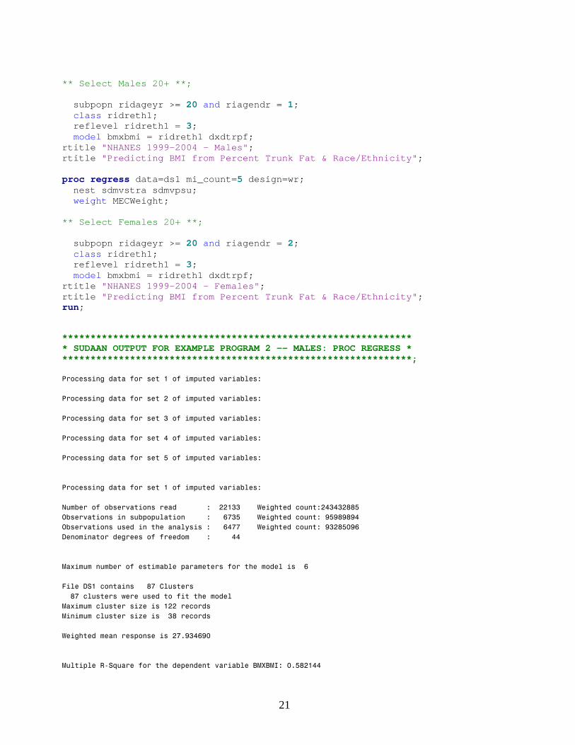
** Select Males 20+ **;
subpopn ridageyr >= 20 and riagendr = 1;class ridreth1;reflevel ridreth1 = 3;model bmxbmi = ridreth1 dxdtrpf;
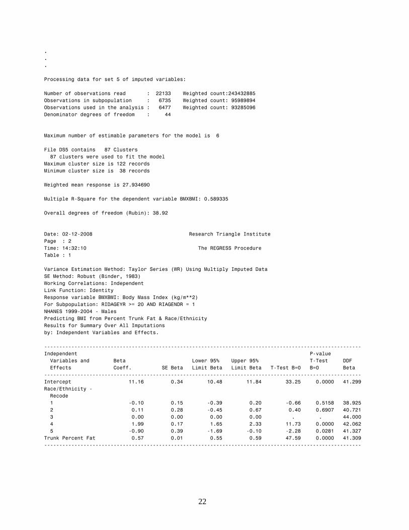
rtitle "NHANES 1999-2004 - Males";rtitle "Predicting BMI from Percent Trunk Fat & Race/Ethnicity";
proc regress data=ds1 mi_count=5 design=wr;nest sdmvstra sdmvpsu;weight MECWeight;
** Select Females 20+ **;
subpopn ridageyr >= 20 and riagendr = 2;class ridreth1;reflevel ridreth1 = 3;model bmxbmi = ridreth1 dxdtrpf;
rtitle "NHANES 1999-2004 - Females";rtitle "Predicting BMI from Percent Trunk Fat & Race/Ethnicity"; run;
************************************************************** * SUDAAN OUTPUT FOR EXAMPLE PROGRAM 2 -- MALES: PROC REGRESS * **************************************************************;
Processing data for set 1 of imputed variables:
Processing data for set 2 of imputed variables:
Processing data for set 3 of imputed variables:
Processing data for set 4 of imputed variables:
Processing data for set 5 of imputed variables:
Processing data for set 1 of imputed variables:
Number of observations read : 22133 Weighted count:243432885 Observations in subpopulation : 6735 Weighted count: 95989894 Observations used in the analysis : 6477 Weighted count: 93285096 Denominator degrees of freedom : 44
Maximum number of estimable parameters for the model is 6
File DS1 contains 87 Clusters 87 clusters were used to fit the model Maximum cluster size is 122 records Minimum cluster size is 38 records
Weighted mean response is 27.934690
Multiple R-Square for the dependent variable BMXBMI: 0.582144
21
---------------------------------------------------------------------------------------------------------
---------------------------------------------------------------------------------------------------------
---------------------------------------------------------------------------------------------------------
.
.
.
Processing data for set 5 of imputed variables:
Number of observations read : 22133 Weighted count:243432885 Observations in subpopulation : 6735 Weighted count: 95989894 Observations used in the analysis : 6477 Weighted count: 93285096 Denominator degrees of freedom : 44
Maximum number of estimable parameters for the model is 6
File DS5 contains 87 Clusters 87 clusters were used to fit the model Maximum cluster size is 122 records Minimum cluster size is 38 records
Weighted mean response is 27.934690
Multiple R-Square for the dependent variable BMXBMI: 0.589335
Overall degrees of freedom (Rubin): 38.92
Date: 02-12-2008 Research Triangle Institute Page : 2 Time: 14:32:10 The REGRESS Procedure Table : 1
Variance Estimation Method: Taylor Series (WR) Using Multiply Imputed Data SE Method: Robust (Binder, 1983) Working Correlations: Independent Link Function: Identity Response variable BMXBMI: Body Mass Index (kg/m**2) For Subpopulation: RIDAGEYR >= 20 AND RIAGENDR = 1 NHANES 1999-2004 - Males Predicting BMI from Percent Trunk Fat & Race/Ethnicity Results for Summary Over All Imputations by: Independent Variables and Effects.
Independent P-value Variables and Beta Lower 95% Upper 95% T-Test DDF Effects Coeff. SE Beta Limit Beta Limit Beta T-Test B=0 B=0 Beta
Intercept 11.16 0.34 10.48 11.84 33.25 0.0000 41.299 Race/Ethnicity - Recode
1 -0.10 0.15 -0.39 0.20 -0.66 0.5158 38.925 2 0.11 0.28 -0.45 0.67 0.40 0.6907 40.721 3 0.00 0.00 0.00 0.00 . . 44.000 4 1.99 0.17 1.65 2.33 11.73 0.0000 42.062 5 -0.90 0.39 -1.69 -0.10 -2.28 0.0281 41.327
Trunk Percent Fat 0.57 0.01 0.55 0.59 47.59 0.0000 41.309
22
-------------------------------------------------------
-------------------------------------------------------
-------------------------------------------------------
Date: 02-12-2008 Research Triangle Institute Page : 3 Time: 14:32:10 The REGRESS Procedure Table : 1
Variance Estimation Method: Taylor Series (WR) Using Multiply Imputed Data SE Method: Robust (Binder, 1983) Working Correlations: Independent Link Function: Identity Response variable BMXBMI: Body Mass Index (kg/m**2) For Subpopulation: RIDAGEYR >= 20 AND RIAGENDR = 1 NHANES 1999-2004 - Males Predicting BMI from Percent Trunk Fat & Race/Ethnicity Results for Summary Over All Imputations by: Contrast.
Contrast Degrees of P-value
Freedom Wald F Wald F
OVERALL MODEL 6 28244.49 0.0000 MODEL MINUS INTERCEPT 5 473.72 0.0000 INTERCEPT . . . RIDRETH1 4 66.03 0.0000 DXDTRPF 1 2265.27 0.0000
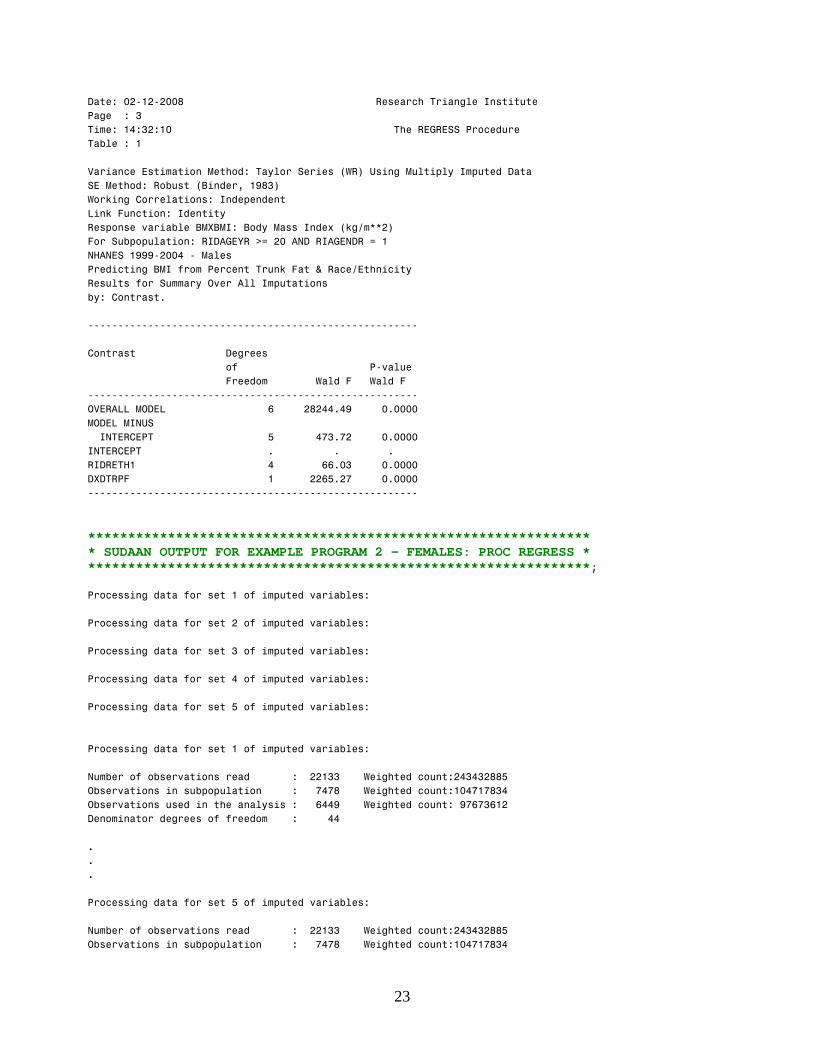
*************************************************************** * SUDAAN OUTPUT FOR EXAMPLE PROGRAM 2 – FEMALES: PROC REGRESS * ***************************************************************;
Processing data for set 1 of imputed variables:
Processing data for set 2 of imputed variables:
Processing data for set 3 of imputed variables:
Processing data for set 4 of imputed variables:
Processing data for set 5 of imputed variables:
Processing data for set 1 of imputed variables:
Number of observations read : 22133 Weighted count:243432885 Observations in subpopulation : 7478 Weighted count:104717834 Observations used in the analysis : 6449 Weighted count: 97673612 Denominator degrees of freedom : 44
.
.
.
Processing data for set 5 of imputed variables:
Number of observations read : 22133 Weighted count:243432885 Observations in subpopulation : 7478 Weighted count:104717834
23
---------------------------------------------------------------------------------------------------------
---------------------------------------------------------------------------------------------------------
Observations used in the analysis : 6449 Weighted count: 97673612 Denominator degrees of freedom : 44
Maximum number of estimable parameters for the model is 6
File DS5 contains 87 Clusters 87 clusters were used to fit the model Maximum cluster size is 118 records Minimum cluster size is 34 records
Weighted mean response is 28.206126
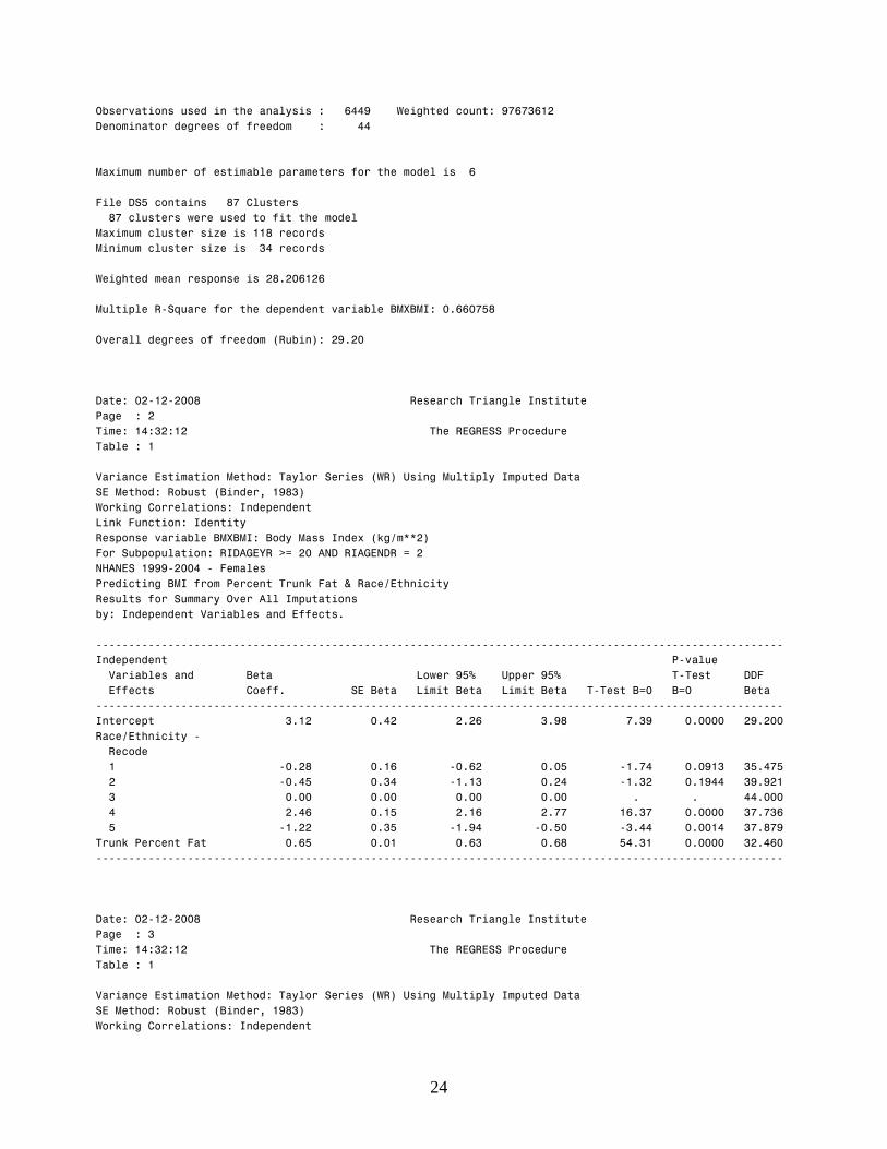
Multiple R-Square for the dependent variable BMXBMI: 0.660758
Overall degrees of freedom (Rubin): 29.20
Date: 02-12-2008 Research Triangle Institute Page : 2 Time: 14:32:12 The REGRESS Procedure Table : 1
Variance Estimation Method: Taylor Series (WR) Using Multiply Imputed Data SE Method: Robust (Binder, 1983) Working Correlations: Independent Link Function: Identity Response variable BMXBMI: Body Mass Index (kg/m**2) For Subpopulation: RIDAGEYR >= 20 AND RIAGENDR = 2 NHANES 1999-2004 - Females Predicting BMI from Percent Trunk Fat & Race/Ethnicity Results for Summary Over All Imputations by: Independent Variables and Effects.
Independent P-value Variables and Beta Lower 95% Upper 95% T-Test DDF Effects--------------------
Coeff. ----------------
SE Beta ------------
Limit Beta -------------
Limit Beta -------------
T-Test B=0 -------------
B=0-----------
Beta -------
Intercept 3.12 0.42 2.26 3.98 7.39 0.0000 29.200 Race/Ethnicity - Recode
1 -0.28 0.16 -0.62 0.05 -1.74 0.0913 35.475 2 -0.45 0.34 -1.13 0.24 -1.32 0.1944 39.921 3 0.00 0.00 0.00 0.00 . . 44.000 4 2.46 0.15 2.16 2.77 16.37 0.0000 37.736 5 -1.22 0.35 -1.94 -0.50 -3.44 0.0014 37.879
Trunk Percent Fat 0.65 0.01 0.63 0.68 54.31 0.0000 32.460
Date: 02-12-2008 Research Triangle Institute Page : 3 Time: 14:32:12 The REGRESS Procedure Table : 1
Variance Estimation Method: Taylor Series (WR) Using Multiply Imputed Data SE Method: Robust (Binder, 1983) Working Correlations: Independent
24
-------------------------------------------------------
-------------------------------------------------------
-------------------------------------------------------
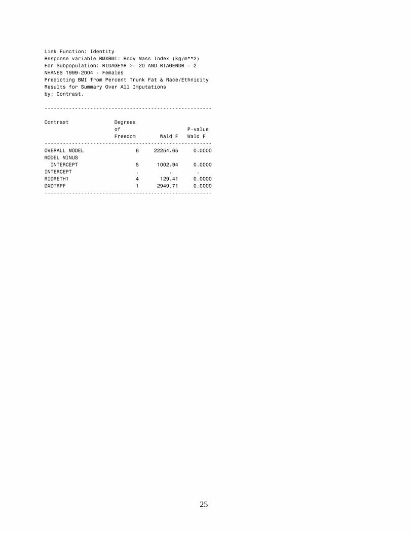
Link Function: Identity Response variable BMXBMI: Body Mass Index (kg/m**2) For Subpopulation: RIDAGEYR >= 20 AND RIAGENDR = 2 NHANES 1999-2004 - Females Predicting BMI from Percent Trunk Fat & Race/Ethnicity Results for Summary Over All Imputations by: Contrast.
Contrast Degrees of P-value
Freedom Wald F Wald F
OVERALL MODEL 6 22254.65 0.0000 MODEL MINUS INTERCEPT 5 1002.94 0.0000 INTERCEPT . . . RIDRETH1 4 129.41 0.0000 DXDTRPF 1 2949.71 0.0000
25

References Barnard J and Rubin DB (1999). Small-sample degrees of freedom with multiple imputation.
Biometrika, 86,948-55.
Baumgartner RN, Heymsfield SB, and Roche AF (1995). Human body composition and the
epidemiology of disease. Obes Res, 3,73-95.
Belsley DA, Kuh E, and Welsch, RE (1980). Regression Diagnostics: Identifying influential data
and sources of collinearity. New York: John Wiley.
Box GEP and Cox DR (1964). An analysis of transformations. J Royal Stat Soc, Ser. B, 26,211–46.
Deurenberg P, Yap M, and van Staveren WA (1998). Body mass index and percent body fat: a
meta analysis among different ethnic groups. Int J Obes Relat Metab Disord, 22,1164-71.
Flegal KM, Carroll MD, Ogden CL, and Johnson CL (2002). Prevalence and trends in obesity
among US adults, 1999-2000. JAMA, 288,1723-27.
Gallagher D, Visser M, Sepulveda D, Pierson RN, Harris T, and Heymsfield SB (1996). How
useful is body mass index for comparison of body fatness across age, sex, and ethnic groups? Am J
Epidemiol, 143,228-39.
Genant HK, Engelke K, Fuerst T, Güer C-C, Grampp S, Harris ST, Jergas M, Lang T, Lu Y,
Majumdar S, Mathur A, and Takada M (1996). Noninvasive assessment of bone mineral and
structure: state of the art. J Bone Miner Res, 11,707-30.
Heymsfield SB, Wang J, Heshka S, Kehayias JJ, and Pierson RN Jr. (1989). Dual-photon
absorptiometry: comparison of bone mineral and soft tissue measurements in vivo with established
methods. Am J Clin Nutr, 49,1283-9.
Kennickell AB (1991). Imputation of the 1989 Survey of Consumer Finances: Stochastic relaxation
and multiple imputation. Proceedings of the Section on Survey Research Methods, American
Statistical Association, 1-10.
26
Li K-H, Meng X-L, Raghunathan TE, and Rubin DB (1991). Significance levels from repeated p-
values with multiply-imputed data. Statistica Sinica, 1,65-92.
Li K-H, Raghunathan TE, and Rubin DB (1991). Large sample significance levels from multiply-
imputed data using moment-based statistics and an F reference distribution. J Amer Stat Assoc,
86,1065-73.
Little, RJA and Raghunathan TE (1997). Should imputation of missing data condition on all
observed variables? Proceedings of the Section on Survey Research Methods, American Statistical
Association, 617-22.
Lohman TG, Chen Z. Dual-Energy X-Ray Absorptiometry. In Human Body Composition-2nd
Edition. Heymsfield SB, Lohman T, Wang Z-M, Going SB, Eds. Human Kinetics,
www.humankinetics.com, 2005.
Looker AC, Wahner HW, Dunn WL, Calvo MS, Harris TB, Heyse SP, Johnston Jr CC, and
Lindsay R (1998). Updated data on proximal femur bone mineral levels of US adults. Osteoporosis
Intl, 8,468-89.
Meng X-L (1994). Multiple-imputation inferences with uncongenial sources of input, Stat Sci,
9,538–58.
Meng X-L and Rubin DB (1992). Performing likelihood ratio tests with multiply-imputed data sets.
Biometrika, 79,103-11.
National Center for Health Statistics (2001). Third National Health and Nutrition Examination
Survey (NHANES III, 1988-1994): Multiply Imputed Data Set. CD-ROM, Series II, No. 7A.
Documentation. Hyattsville, MD: Centers for Disease Control and Prevention, U.S. Department of
Health and Human Services. Available at
http://www.cdc.gov/nchs/about/major/nhanes/datalink.htm.
Njeh CF, Fuerst T, Hans D, Blake GM, and Genant HK (1990). Radiation exposure in bone mineral
density assessment. Appl Radiat Isot, 50,215-36.
27
Ogden CL, Flegal KM, Carroll MD, and Johnson CL (2002). Prevalence and trends in overweight
among US children and adolescents, 1999-2000. JAMA, 288,1728-32.
Ogden CL, Carroll MD, Curtin LR, McDowell MA, Tabak CJ, and Flegal KM (2006). Prevalence
of overweight and obesity in the United States, 1999-2004. JAMA, 295,1549-55.
Pedlow S, Luke JV, and Blumberg SJ (2007). Multiple Imputation of Missing Household Poverty
Level Values from the National Survey of Children with Special Health Care Needs, 2001, and the
National Survey of Children’s Health, 2003. Hyattsville, MD: Survey Planning and Special
Surveys Branch, Division of Health Interview Statistics, National Center for Health Statistics,
Centers for Disease Control and Prevention, U.S. Department of Health and Human Services.
http://www.cdc.gov/nchs/data/slaits/mimp01_03.pdf.
Raghunathan TE, Lepkowski JW, Van Hoewyk J, and Solenberger P (2001). A multivariate
technique for multiply imputing missing values using a sequence of regression models. Surv Meth,
27,85-95.
Raghunathan TE, Solenberger P, and Van Hoewyk J (2002). IVEware: Imputation and Variance
Estimation Software Users Guide. University of Michigan: Survey Research Center, Institute for
Social Research.
Royston P (2005). Multiple imputation of missing values: Update of ice. Stata Journal, 5,527-36.
Rubin DB (1978). Multiple imputation in sample surveys – a phenomenological Bayesian approach
to nonresponse. Proceedings of the Section on Survey Research Methods, American Statistical
Association, 20-34.
Rubin DB (1987). Multiple Imputation for Nonresponse in Surveys. New York: John Wiley.
Rubin DB (1996). Multiple imputation after 18+ years. J Amer Stat Assoc, 91,473-489.
Rubin DB and Schenker N (1986). Multiple imputation for interval estimation from simple random
samples with ignorable nonresponse. J Amer Stat Assoc, 81,366-74.
28

Schenker N, Raghunathan TE, Chiu P-L, Makuc DM, Zhang G, and Cohen AJ (2006). Multiple
imputation of missing income data in the National Health Interview Survey. J Amer Stat Assoc,
101,924-33.
Thomas SR, Kalkwarf HJ, Buckley DD, and Heubi JE (2005). Effective dose of dual-energy x-ray
absorptiometry scans in children as a function of age. J Clin Densitometry, 8,415-22.
Tothill P, Han TS, Avenell A, McNeill G, and Reid DM (1996). Comparisons between fat
measurements by dual-energy x-ray absorptiometry, underwater weighing and magnetic resonance
imaging in healthy women. Eur J Clin Nutr, 50,747-752.
Van Buuren S, Brand J, Groothuis-Oudshoorn C, and Rubin D (2006). Fully conditional
specification in multivariate imputation. J Stat Comp Sim, 76,1049-1064.
Van Buuren S and Oudshoorn CGM (1999). Flexible multivariate imputation by MICE. Leiden:
TNO Preventie en Gezondheid, TNO/VGZ/PG 99.054.
Wahner HW and Fogelman I (1994). The Evaluation of Osteoporosis: Dual Energy X-ray
Absorptiometry in Clinical Practice. Martin Dunitz Publishers.
WHO Technical Report Series. (1994) Assessment of fracture risk and its application to screening
for post menopausal osteoporosis. World Health Organization, Geneva., 843.
WHO Technical Report Series. (1995) Physical Status: the use and interpretation of
anthropometry: report of a WHO expert committee. World Health Organization, Geneva., 854,1
452.
29
Table 1. Percentages of survey participants in 1999-2004 with data missing for one or more regions
by age group.
Table 2. Percentages of survey participants in 1999-2004 with data missing for one or more regions
by body mass index (BMI) category.
30
Table 3. DXA variables included in the imputation model.
Name of Original Variable Description
DXDLAA Left Arm Area (cm^2) DXDLABMC Left Arm BMC (g) DXDLAFAT Left Arm Fat (g) DXDLALER Left Arm Lean excl BMC (g) DXDRAA Right Arm Area (cm^2) DXDRABMC Right Arm BMC (g) DXDRAFAT Right Arm Fat (g) DXDRALER Right Arm Lean excl BMC (g) DXDTRFAT Truncal fat (g) XDTRLER Trunk Lean excl BMC (g) DXDLLA Left Leg Area (cm^2) DXDLLBMC Left Leg BMC (g) DXDLLFAT Left Leg Fat (g) DXDLLLER Left Leg Lean excl BMC (g) DXDRLA Right Leg Area (cm^2) DXDRLBMC Right Leg BMC (g) DXDRLFAT Right Leg Fat (g) DXDRLLER Right Leg Lean excl BMC (g) DXDHEA Head Area (cm^2) DXDHEBMC Head Bone Mineral Content (g) DXDHEFAT Head Fat (g) DXDHELER Head Lean excl BMC (g) DXDLRA Left Ribs Area (cm^2) DXDLRBMC Left Ribs BMC (g) DXDRRA Right Ribs Area (cm^2) DXDRRBMC Right Ribs BMC (g) DXDTSA Thoracic Spine Area (cm^2) DXDTSBMC Thoracic Spine BMC (g) DXDLSA Lumbar Spine Area (cm^2) DXDLSBMC Lumbar Spine BMC (g) DXDPEA Pelvis Area (cm^2) DXDPEBMC Pelvis BMC (g)
31
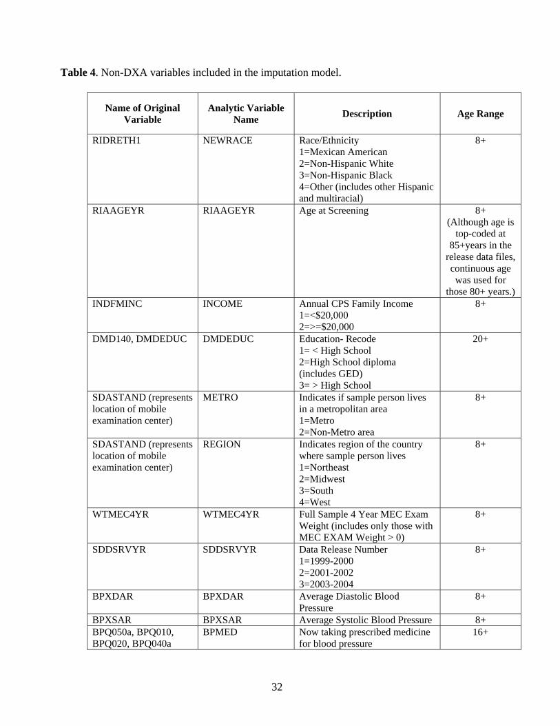
Table 4. Non-DXA variables included in the imputation model.
Name of Original Variable
Analytic Variable Name Description Age Range
RIDRETH1 NEWRACE Race/Ethnicity 1=Mexican American 2=Non-Hispanic White 3=Non-Hispanic Black 4=Other (includes other Hispanic and multiracial)
8+
RIAAGEYR RIAAGEYR Age at Screening 8+ (Although age is
top-coded at 85+years in the
release data files, continuous age was used for
those 80+ years.) INDFMINC INCOME Annual CPS Family Income
1=<$20,000 2=>=$20,000
8+
DMD140, DMDEDUC DMDEDUC Education- Recode 1= < High School 2=High School diploma (includes GED) 3= > High School
20+
SDASTAND (represents location of mobile examination center)
METRO Indicates if sample person lives in a metropolitan area 1=Metro 2=Non-Metro area
8+
SDASTAND (represents location of mobile examination center)
REGION Indicates region of the country where sample person lives 1=Northeast 2=Midwest 3=South 4=West
8+
WTMEC4YR WTMEC4YR Full Sample 4 Year MEC Exam Weight (includes only those with MEC EXAM Weight > 0)
8+
SDDSRVYR SDDSRVYR Data Release Number 1=1999-2000 2=2001-2002 3=2003-2004
8+
BPXDAR BPXDAR Average Diastolic Blood Pressure
8+
BPXSAR BPXSAR Average Systolic Blood Pressure 8+ BPQ050a, BPQ010, BPQ020, BPQ040a
BPMED Now taking prescribed medicine for blood pressure
16+
32
1=yes 2=no
BMXWT BMXWT Weight (kg) 8+ BMXARMC BMXARMC Arm Circumference (cm) 8+ BMXSUB BMXSUB Subscapular Skinfold (mm) 8+ BMXTRI BMXTRI Triceps Skinfold (mm) 8+ BMXWAIST BMXWAIST Waist Circumference (cm) 8+ BMXHT BMXHT Height (cm) 8+ BMXWAIST_BMXHT BMXWAIST_BMX
HT Waist Circumference (cm)/Height (cm)
8+
BMXBMI BMXBMI Body Mass Index (kg/m**2) 8+ BMXBMI OBESEIND 3 BMI categories
1=Under or normal weight <25 2=Overweight 25-<30 3=Obese >=30
20+
DIQ010 DRDIAB# Doctor told you have diabetes 1=yes 2=no (DIQ010=2 or 3)
8+
HUQ010 HEALTHSTAT General Health Condition 1=excellent/very good 2=good 3=fair/poor
8+
LBXTC LBXTC Total Cholesterol (mg/dL) 8+ LBDHDL LBDHDL HDL Cholesterol (mg/dL) 8+ LBXSTR*** LBXSTR Natural Log Trigylcerides
(mg/dL) –nonfasting 12+
BPQ100D, BPQ060, BPQ080, BPQ090d
CHOLMED Now taking prescribed medicine for cholesterol 1=yes 2=no
20+
PAD200, PAD320 PHYSICALACTIVI TY
Moderate or Vigorous Activity past 30 days 1=yes 2=no
12+
SMQ620, SMD630, SMQ640, SMQ020, SMQ040
SMOKER Smoking Status 1=Never 2=Former 3=Current
12+
OSQ030aa to OSQ030cf, OSQ010a, OSQ010b, OSQ010c
FRACTURE Experienced a fracture 1=yes 2=no
20+
MCQ250e, MCQ260ea, MCQ260eb
FAMOSTEO Family History of Osteoporosis 1=yes 2=no
20+
RHQ420, RHQ440, RHQ510, RHQ520
BCEVER Ever take birth control 1=yes 2=no
Females 12+
RHQ030, RHQ040, RHQ310, RHQ050, RHQ060, RHQ340,
NEWMENO Menopause Status 1=Premenopausal 2=Menopause Transition
Females 12+
33

RHQ290 3=Surgical/ Medical Amenorrhea 4=Natural Menopause
RHQ554, RHQ570, RHQ580, RHQ596, RHQ540
ANYEST Ever take non-birth control estrogen 1=yes 2=no
Females 20+
ALCDRNKYR DRNKYR_CAT Categories for average alcohol consumption per year 0=none 1=Less than once a week 2=Less than once a day 3=Once a day or more
20+
Nhcode in (01900, 51500, 50900, 09400)
OSTEORX Osteoporosis Treatments: alendronate, risedronate, raloxifene, calcitonin 1=yes 0=no
8+
fdacode =1374 ANTICONV Anticonvulsants 1=yes 0=no
8+
Nhcode in (16400 17500 25300 31000 39600 39700 48600 49000 58100 58300 36100 56300 36200 38700 50100 56300 92400)
PRESMEDS Prescription Meds: Cortisone, Thyroid, levothyroxine, liotrix, methimazole, propylthiouracil 1=yes 0=no
8+
DSD010, DSDANTA ANTACID Antacids (of those who answered yes/no to dietary supplement) 1=took antacid past month 2=did not take antacid past month
8+
DSD010 DSD0101 Any dietary supplements taken? 1=yes 2=no
8+
DBD196 DBD196_NEW Past 30 day milk consumption recode 1=Never/Rarely less than once a week 2=Sometimes/Often/Varies
8+
DRXTCALC, DRXTPROT, DRDTSODI, DRXTPOTA, DRXTVC, DRXTZINC, DRXTMAGN, DRXTCOPP, DRXTIRON, DRXTCAFF
DRXTCALC, DRXTPROT, DRDTSODI, DRXTPOTA, DRXTVC, DRXTZINC, DRXTMAGN, DRXTCOPP, DRXTIRON, DRXTCAFF DRXTTFAT
Diet: Calcium, protein, sodium, potassium, vitamin C, zinc, magnesium, copper, iron, caffeine, total fat
8+
34
35
Figure 1
Total DXA Weight (g) versus Measured Scale Weight (kg) First Imputation for Males 20-39
Observed 1 or More Imputations
Tota
l DXA
Wei
ght (
g)
40,000
50,000
60,000
70,000
80,000
90,000
100,000
110,000
120,000
130,000
140,000
150,000
160,000
170,000
180,000
190,000
200,000
210,000
Measured Scale Weight (kg)
40 50 60 70 80 90 100 110 120 130 140 150 160 170 180 190 200
Figure 2
Total DXA Weight (g) versus Body Mass Index (BMI) First Imputation for Males 20-39
210,000 Observed 200,000 1 or More Imputations
190,000
180,000
170,000
160,000
150,000
140,000
130,000
120,000
110,000
100,000
90,000
80,000
70,000
60,000
50,000
40,000
10 20 30 40 50 60
Body Mass Index (kg/m**2)
Tota
l DXA
Wei
ght (
g)
36
70

Figure 3
Trunk Fat from DXA versus Waist Circumference First Imputation for Males 20-39
50,000 Observed Imputed
40,000
30,000
20,000
10,000
0
60 70 80 90 100 110 120 130 140 150 160 170 180
Waist Circumference (cm)
Trun
k Fa
t (g)
37
500
Figure 4
Left versus Right Arm Bone Mineral Content First Imputation for Males 20-39
Observed Left Imputed Right Imputed Both Imputed
400
300
200
100
100 200 300 400 500
Right Arm BMC (g)
Left
Arm
BM
C (g
)
38

Figure 5
39