NBER WORKING PAPER SERIES

MORAL HAZARD VS. LIQUIDITY AND OPTIMAL UNEMPLOYMENT INSURANCE

Raj Chetty

Working Paper 13967http://www.nber.org/papers/w13967

NATIONAL BUREAU OF ECONOMIC RESEARCH1050 Massachusetts Avenue

Cambridge, MA 02138April 2008

I have benefited from discussions with Joseph Altonji, Alan Auerbach, Olivier Blanchard, RichardBlundell, David Card, Liran Einav, Martin Feldstein, Amy Finkelstein, Jon Gruber, Jerry Hausman,Caroline Hoxby, Juan Jimeno, Kenneth Judd, Lawrence Katz, Patrick Kline, Bruce Meyer, Ariel Pakes,Luigi Pistaferri, Emmanuel Saez, Jesse Shapiro, Robert Shimer, Adam Szeidl, Ivan Werning, anonymousreferees, and numerous seminar participants. Philippe Bouzaglou, Greg Bruich, David Lee, Ity Shurtz,Jim Sly, and Philippe Wingender provided excellent research assistance. I am very grateful to JulieCullen and Jon Gruber for sharing their unemployment benefit calculator, and to Suzanne Simonettaand Loryn Lancaster at the Dept. of Labor for assistance with state UI laws. Funding from the NationalScience Foundation and NBER is gratefully acknowledged. The data and code used for the empiricalanalysis and numerical simulations are available on the author's website. The views expressed hereinare those of the author(s) and do not necessarily reflect the views of the National Bureau of EconomicResearch.

NBER working papers are circulated for discussion and comment purposes. They have not been peer-reviewed or been subject to the review by the NBER Board of Directors that accompanies officialNBER publications.

© 2008 by Raj Chetty. All rights reserved. Short sections of text, not to exceed two paragraphs, maybe quoted without explicit permission provided that full credit, including © notice, is given to the source.

Moral Hazard vs. Liquidity and Optimal Unemployment InsuranceRaj ChettyNBER Working Paper No. 13967April 2008JEL No. H0,J6

ABSTRACT

This paper presents new evidence on why unemployment insurance (UI) benefits affect search behaviorand develops a simple method of calculating the welfare gains from UI using this evidence. I showthat 60 percent of the increase in unemployment durations caused by UI benefits is due to a "liquidityeffect" rather than distortions in marginal incentives to search ("moral hazard") by combining twoempirical strategies. First, I find that increases in benefits have much larger effects on durations forliquidity constrained households. Second, lump-sum severance payments increase durations substantiallyamong constrained households. I derive a formula for the optimal benefit level that depends only onthe reduced-form liquidity and moral hazard elasticities. The formula implies that the optimal UI benefitlevel exceeds 50 percent of the wage. The "exact identification" approach to welfare analysis proposedhere yields robust optimal policy results because it does not require structural estimation of primitives.

Raj ChettyDepartment of EconomicsUC, Berkeley521 Evans Hall #3880Berkeley, CA 94720and NBERchetty@econ.berkeley.edu

1 Introduction

One of the classic empirical results in public �nance is that social insurance programs such as

unemployment insurance (UI) reduce labor supply. For example, Mo¢ tt (1985), Meyer (1990),

and others have shown that a 10% increase in unemployment bene�ts raises average unemployment

durations by 4-8% in the U.S. This �nding has traditionally been interpreted as evidence of moral

hazard caused by a substitution e¤ect: UI distorts the relative price of leisure and consumption,

reducing the marginal incentive to search for a job. For instance, Krueger and Meyer (2002, p2328)

remark that behavioral responses to UI and other social insurance programs are large because they

�lead to short-run variation in wages with mostly a substitution e¤ect.� Similarly, Gruber (2007,

p395) notes that �UI has a signi�cant moral hazard cost in terms of subsidizing unproductive

leisure.�

This paper questions whether the link between unemployment bene�ts and durations is purely

due to moral hazard. The analysis is motivated by evidence that many unemployed individuals

have limited liquidity and exhibit excess sensitivity of consumption to cash-on-hand (Gruber 1997,

Browning and Crossley 2001, Bloemen and Stancanelli 2005). Indeed, nearly half of job losers in

the United States report zero liquid wealth at the time of job loss, suggesting that many households

may be unable to smooth transitory income shocks relative to permanent income.

Using a job search model with incomplete credit and insurance markets, I show that when

an individual cannot smooth consumption perfectly, unemployment bene�ts a¤ect search intensity

through a �liquidity e¤ect� in addition to the moral hazard channel emphasized in earlier work.

Intuitively, UI bene�ts increase cash-on-hand and consumption while unemployed for an agent who

cannot smooth perfectly. Such an agent faces less pressure to �nd a new job quickly, leading to

a longer duration. Hence, unemployment bene�ts raise durations purely through moral hazard

when consumption can be smoothed perfectly, but through both liquidity and moral hazard e¤ects

when smoothing is imperfect.1

The distinction between liquidity and moral hazard is of interest because the two e¤ects have

divergent implications for the welfare consequences of UI. The substitution e¤ect is a socially

suboptimal response to the creation of a wedge between private and social marginal costs. In

contrast, the liquidity e¤ect is a socially bene�cial response to the correction of the credit and

1 I use the term �liquidity e¤ect�to refer to the e¤ect of a wealth grant while unemployed. The liquidity e¤ect di¤ersfrom the wealth e¤ect (i.e., an increase permanent income) if the agent cannot smooth consumption perfectly. Indeed,there are models where the wealth e¤ect is zero but the liquidity e¤ect is positive because of liquidity constraints (seee.g. Shimer and Werning 2007).

1

insurance market failures. Building on this logic, I develop a new formula for the optimal unem-

ployment bene�t level that depends purely on the liquidity and moral hazard e¤ects. The formula

uses revealed preference to calculate the welfare gain from insurance: if an agent chooses a longer

duration primarily because he has more cash-on-hand (as opposed to distorted incentives), we infer

that UI bene�ts bring the agent closer to the social optimum.

The approach to welfare analysis proposed in this paper is very di¤erent from the traditional

approach of structurally estimating a model�s primitives (curvature of utility, borrowing limit,

etc.) and then numerically simulating the e¤ects of policy changes. I instead identify a pair of

reduced-form elasticities that serve as su¢ cient statistics for welfare analysis. Conditional on these

elasticities, the primitives do not need to be identi�ed because any combination of primitives that

matches the elasticities leads to the same welfare results. In this sense, the structural approach is

�over-identi�ed�for the purpose of welfare analysis, whereas the method proposed here is �exactly

identi�ed.� In addition to simplicity, the exact identi�cation approach has two advantages. First,

it is less model dependent. While previous studies of unemployment insurance have had to make

stark assumptions about borrowing constraints and the lack of private insurance (e.g. Wolpin 1987;

Hansen and Imrohoglu 1992), the formula here requires no such assumptions. Second, it is likely to

be more empirically credible. Since one has to identify two parameters rather than a large number

of primitives, it is feasible to estimate the relevant elasticities using quasi-experimental variation

and relatively few parametric assumptions.2

I implement this method empirically by estimating the importance of moral hazard vs. liquidity

in UI using two complementary strategies. I �rst estimate the e¤ect of unemployment bene�ts on

durations separately for liquidity constrained and unconstrained households, exploiting di¤erential

changes in bene�t levels across states in the U.S. Since households�ability to smooth consumption

is unobserved, I proxy for it using three measures: asset holdings, single vs. dual-earner status, and

an indicator for having to make a mortgage payment. I �nd that a 10% increase in UI bene�ts

raises unemployment durations by 7-10% in the constrained groups. In contrast, changes in UI

bene�ts have much smaller e¤ects on durations in the unconstrained groups, indicating that the

moral hazard e¤ect is relatively small among these groups. These results suggest that liquidity

e¤ects could be quite important in the bene�ts-duration link. However, they do not directly

establish that bene�ts raise the durations of constrained agents by increasing liquidity unless one

2The disadvantage of exact identi�cation is that the scope of questions for which it can be used is limited. Seesection 2.5 for a detailed comparison of the two approaches.

2

assumes that the substitution elasticities are similar across constrained and unconstrained groups.

To avoid identi�cation from cross-sectional comparisons between di¤erent types of job losers,

I pursue a second empirical strategy to estimate the magnitude of the liquidity e¤ect. I exploit

variation across job losers in the receipt of lump-sum severance payments, which provide liquidity

but have no moral hazard e¤ect. Using a survey of job losers from Mathematica containing

information on severance pay, I �nd that individuals who received severance pay (worth about

$4000 on average) have substantially longer durations. An obvious concern is that this �nding

may re�ect correlation rather than causality because severance pay is not randomly assigned. Three

pieces of evidence support the causality of severance pay. First, severance payments have a large

e¤ect on durations among constrained (low asset) households, but have no e¤ect on durations among

unconstrained households. Second, the estimated e¤ect of severance pay is not a¤ected by controls

for demographics, income, job tenure, industry, and occupation in a Cox hazard model. Third,

individuals who receive larger severance amounts have longer unemployment durations. These

�ndings, though not conclusive given the lack of randomized variation in cash grants, suggest that

UI has a substantial liquidity e¤ect.

Combining the point estimates from the two empirical approaches, I �nd that roughly 60% of the

marginal e¤ect of UI bene�ts on durations is due to the liquidity e¤ect. Coupled with the formula

derived from the search model, this estimate implies that the marginal welfare gain of increasing

the unemployment bene�t level from the prevailing rate of 50% of the pre-unemployment wage is

small but positive. Hence, the optimal bene�t level exceeds 50% of the wage in the existing UI

system that pays constant bene�ts for six months. An important caveat to this policy conclusion

is that it does not consider other types of policy instruments to resolve credit and insurance market

failures. A natural alternative tool to resolve credit market failures is the provision of loans. I

brie�y compare the potential value of loans vs. UI bene�ts using numerical simulations at the end

of the paper.

In addition to the empirical literature on unemployment insurance, this paper relates to and

builds on several other strands of the literature in macroeconomics and public �nance. First,

several studies have used consumption data to investigate the importance of liquidity constraints

and partial insurance (see e.g., Zeldes 1989; Johnson, Parker, and Souleles 2006; Blundell, Pistaferri,

and Preston 2008). This paper presents analogous evidence from the labor market, showing that

labor supply is �excessively sensitive�to transitory income because of imperfections in credit and

insurance markets. Second, several studies have explored the e¤ects of incomplete insurance and

3

credit markets for job search behavior and UI using simulations of calibrated search models (Hansen

and Imrohoglu 1992; Acemoglu and Shimer 2000). The analysis here can be viewed as the empirical

counterpart of such studies, in which the extent to which agents can smooth shocks is estimated

empirically rather than simulated from a calibrated model.

The distinction between moral hazard and liquidity e¤ects arises in any private or social insur-

ance program, and could be used to calculate the value of insuring other shocks such as health or

disability. More generally, it may be possible to develop similar exact identi�cation strategies to

characterize the welfare consequences of other government policies beyond social insurance.

The paper proceeds as follows. The search model and formula for optimal bene�ts are presented

in the next section. Section 3 discusses the evidence on heterogeneous e¤ects of unemployment

bene�ts on durations. Section 4 examines the e¤ect of severance payments on durations. The

estimates are used to calibrate the formula for welfare gains in section 5. Section 6 concludes.

2 Theory

I analyze a job search model closely related to the models in Chetty (2003), Lentz and Tranaes

(2005), and Card, Chetty, and Weber (2007). The model features (partial) failures in credit and

insurance markets, creating a potential role for government intervention via an insurance program.

I �rst distinguish the moral hazard and liquidity e¤ects of UI and then derive a formula for the

welfare gain from UI in terms of these elasticities.

2.1 Agent and Planner�s Problems

Agent�s Problem. Consider a discrete-time setting where the agent lives for T periods f0; :::; T �1g.

Assume that the interest rate and the agent�s time discount rate are zero. Suppose the agent

becomes unemployed at t = 0. An agent who enters a period t without a job �rst chooses search

intensity st. Normalize st to equal the probability of �nding a job in the current period. Let (st)

denote the cost of search e¤ort, which is strictly increasing and convex. If search is successful, the

agent begins working immediately in period t.3 Assume that all jobs last inde�nitely once found.

I make three assumptions to simplify the exposition in the baseline case: (1) the agent earns

a �xed pre-tax wage of wt if employed in period t, eliminating reservation-wage choices; (2) assets

3A more conventional timing assumption in search models without savings is that search in period t leads to a jobthat begins in period t+ 1. Assuming that search in period t leads to a job in period t itself simpli�es the analyticexpressions for @st

@At, as shown by Lentz and Tranaes (2005).

4

prior to job loss (A0) are exogenous, eliminating e¤ects of UI bene�ts on savings behavior prior to

job loss; and (3) no heterogeneity across agents. These assumptions are relaxed in the extensions

analyzed in section 2.4.

If the worker is unemployed in period t, he receives an unemployment bene�t bt < wt. If the

worker is employed in period t, he pays a tax � that is used to �nance the unemployment bene�t.

Let cet denote the agent�s consumption in period t if a job is found in that period. If the agent fails

to �nd a job in period t, he sets consumption to cut . The agent then enters period t+1 unemployed

and the problem repeats.

Let v(ct) denote �ow consumption utility if employed in period t and u(ct) denote �ow con-

sumption utility if unemployed. Assume that u and v are strictly concave. Note that this utility

speci�cation permits arbitrary complementarities between consumption and labor.

Search Behavior. The value function for an individual who �nds a job at the beginning of period

t, conditional on beginning the period with assets At is

Vt(At) = maxAt+1�L

v(At �At+1 + wt � �) + Vt+1(At+1). (1)

where L is a lower bound on assets. The value function for an individual who fails to �nd a job at

the beginning of period t and remains unemployed is

Ut(At) = maxAt+1�L

u(At �At+1 + bt) + Jt+1(At+1) (2)

where

Jt(At) = maxst

stVt(At) + (1� st)Ut(At)� (st) (3)

is the value of entering period t without a job with assets At. It is easy to show that Vt is

concave because there is no uncertainty following re-employment; however, Ut could be convex. In

simulations of the model with plausible parameters (described below), non-concavity never arises.4

Therefore, I simply assume that Ut is concave in the parameter space of interest.

An unemployed agent chooses st to maximize expected utility at the beginning of period t,

given by (3). Optimal search intensity is determined by the �rst-order condition

0(st) = Vt(At)� Ut(At). (4)

4Lentz and Tranaes (2005) also report that non-concavity never arises in their simulations. They also show thatany non-concavities in Ut can be eliminated by introducing a wealth lottery prior to the choice of st.

5

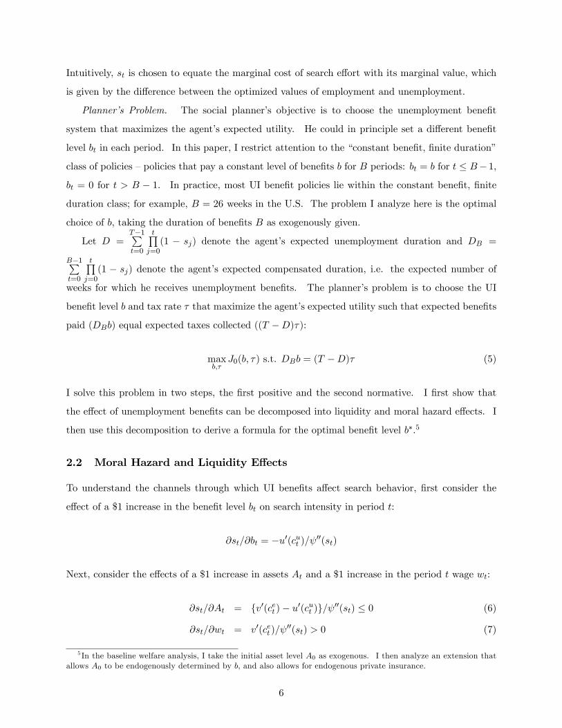
Intuitively, st is chosen to equate the marginal cost of search e¤ort with its marginal value, which

is given by the di¤erence between the optimized values of employment and unemployment.

Planner�s Problem. The social planner�s objective is to choose the unemployment bene�t

system that maximizes the agent�s expected utility. He could in principle set a di¤erent bene�t

level bt in each period. In this paper, I restrict attention to the �constant bene�t, �nite duration�

class of policies �policies that pay a constant level of bene�ts b for B periods: bt = b for t � B� 1;

bt = 0 for t > B � 1. In practice, most UI bene�t policies lie within the constant bene�t, �nite

duration class; for example, B = 26 weeks in the U.S. The problem I analyze here is the optimal

choice of b, taking the duration of bene�ts B as exogenously given.

Let D =T�1Pt=0

tQj=0(1 � sj) denote the agent�s expected unemployment duration and DB =

B�1Pt=0

tQj=0(1 � sj) denote the agent�s expected compensated duration, i.e. the expected number of

weeks for which he receives unemployment bene�ts. The planner�s problem is to choose the UI

bene�t level b and tax rate � that maximize the agent�s expected utility such that expected bene�ts

paid (DBb) equal expected taxes collected ((T �D)�):

maxb;�

J0(b; �) s.t. DBb = (T �D)� (5)

I solve this problem in two steps, the �rst positive and the second normative. I �rst show that

the e¤ect of unemployment bene�ts can be decomposed into liquidity and moral hazard e¤ects. I

then use this decomposition to derive a formula for the optimal bene�t level b�.5

2.2 Moral Hazard and Liquidity E¤ects

To understand the channels through which UI bene�ts a¤ect search behavior, �rst consider the

e¤ect of a $1 increase in the bene�t level bt on search intensity in period t:

@st=@bt = �u0(cut )= 00(st)

Next, consider the e¤ects of a $1 increase in assets At and a $1 increase in the period t wage wt:

@st=@At = fv0(cet )� u0(cut )g= 00(st) � 0 (6)

@st=@wt = v0(cet )= 00(st) > 0 (7)

5 In the baseline welfare analysis, I take the initial asset level A0 as exogenous. I then analyze an extension thatallows A0 to be endogenously determined by b, and also allows for endogenous private insurance.

6

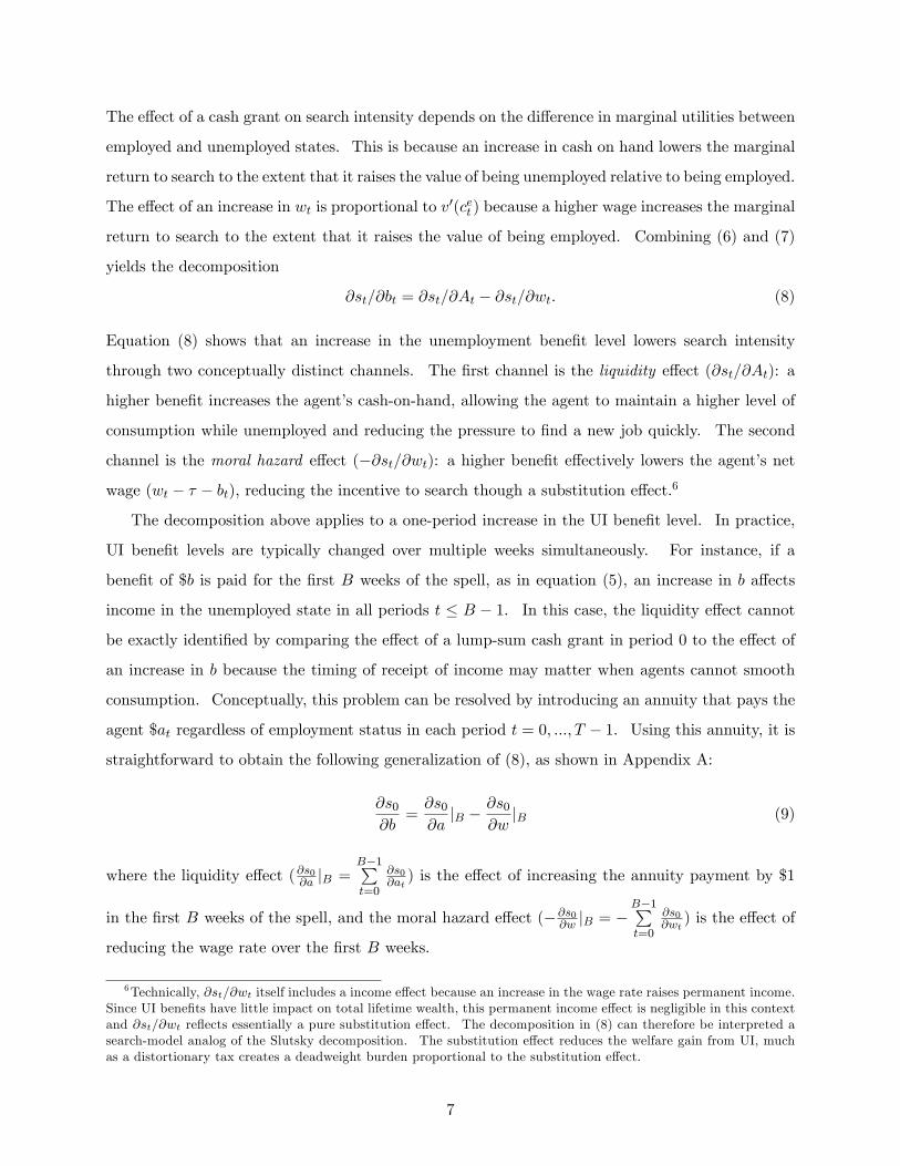
The e¤ect of a cash grant on search intensity depends on the di¤erence in marginal utilities between

employed and unemployed states. This is because an increase in cash on hand lowers the marginal

return to search to the extent that it raises the value of being unemployed relative to being employed.

The e¤ect of an increase in wt is proportional to v0(cet ) because a higher wage increases the marginal

return to search to the extent that it raises the value of being employed. Combining (6) and (7)

yields the decomposition

@st=@bt = @st=@At � @st=@wt. (8)

Equation (8) shows that an increase in the unemployment bene�t level lowers search intensity

through two conceptually distinct channels. The �rst channel is the liquidity e¤ect (@st=@At): a

higher bene�t increases the agent�s cash-on-hand, allowing the agent to maintain a higher level of

consumption while unemployed and reducing the pressure to �nd a new job quickly. The second

channel is the moral hazard e¤ect (�@st=@wt): a higher bene�t e¤ectively lowers the agent�s net

wage (wt � � � bt), reducing the incentive to search though a substitution e¤ect.6

The decomposition above applies to a one-period increase in the UI bene�t level. In practice,

UI bene�t levels are typically changed over multiple weeks simultaneously. For instance, if a

bene�t of $b is paid for the �rst B weeks of the spell, as in equation (5), an increase in b a¤ects

income in the unemployed state in all periods t � B � 1. In this case, the liquidity e¤ect cannot

be exactly identi�ed by comparing the e¤ect of a lump-sum cash grant in period 0 to the e¤ect of

an increase in b because the timing of receipt of income may matter when agents cannot smooth

consumption. Conceptually, this problem can be resolved by introducing an annuity that pays the

agent $at regardless of employment status in each period t = 0; :::; T � 1. Using this annuity, it is

straightforward to obtain the following generalization of (8), as shown in Appendix A:

@s0@b

=@s0@ajB �

@s0@w

jB (9)

where the liquidity e¤ect (@s0@a jB =B�1Pt=0

@s0@at) is the e¤ect of increasing the annuity payment by $1

in the �rst B weeks of the spell, and the moral hazard e¤ect (�@s0@w jB = �

B�1Pt=0

@s0@wt) is the e¤ect of

reducing the wage rate over the �rst B weeks.

6Technically, @st=@wt itself includes a income e¤ect because an increase in the wage rate raises permanent income.Since UI bene�ts have little impact on total lifetime wealth, this permanent income e¤ect is negligible in this contextand @st=@wt re�ects essentially a pure substitution e¤ect. The decomposition in (8) can therefore be interpreted asearch-model analog of the Slutsky decomposition. The substitution e¤ect reduces the welfare gain from UI, muchas a distortionary tax creates a deadweight burden proportional to the substitution e¤ect.

7

Empirical Implications: Heterogeneous Responses. The prevailing view in the existing literature

is that individuals take longer to �nd a job when receiving higher UI bene�ts solely because of the

lower private return to work. This pure moral hazard interpretation is valid only for an agent who

has access to perfect credit and insurance markets. Since such an agent sets v0(ce0) = v0(cet ) = u0(cut )

for all t, the liquidity e¤ect @s0@a jB = 0 because an annuity payment raises Vt(At) and Ut(At) by the

same amount.7 At the other extreme, a hand-to-mouth consumer who sets consumption equal to

income has v0(cet )� u0(cut ) < 0. Since this agent experiences large �uctuations in marginal utility

across states, the magnitude of @s0@a jB can be large for him.

More generally, between the hand-to-mouth and perfect-smoothing extremes, individuals who

have less ability to smooth will exhibit larger liquidity and total UI bene�t e¤ects holding all else

constant. To illustrate this heterogeneity, I numerically simulate the search model for agents with

di¤erent levels of initial assets. I parametrize the search model using CRRA utility (u(c) = v(c) =

c1�

1� ) and a convex disutility of search e¤ort ( (s) = � s1+�

1+� ).8 I set = 1:75, � = 0:1, � = 5, and

w = $340 per week. The asset limit is L = �$1000 and T = 500 (10 years). The UI bene�t

bt = b is constant for B = 26 weeks. Finally, assume that the agent receives a baseline annuity

payment of at = 0:25w = $85 in each period, which can be interpreted as the income of a secondary

earner. At the median initial asset level of $100 and weekly UI bene�t level of b = 0:5w = 170, this

combination of parameters is roughly consistent with the three key empirical moments used in the

welfare calculation in section 5: the average UI-compensated unemployment duration (data: 15.8

weeks, simulation: 15.8 weeks), the ratio of the liquidity e¤ect to the moral hazard e¤ect (data:

1.50, simulation: 1.35), and the elasticity of unemployment duration with respect to the bene�t

level (data: 0.54, simulation: 0.36).

The solid curves in Figure 1 plot search intensity in period 0 (s0) vs. the UI bene�t level b for

agents with A0 = �$1; 000 and A0 = $13; 000, the 25th and 75th percentiles of the initial asset

distribution of the job losers observed in the data. As predicted, the e¤ect of UI bene�ts on search

intensity falls with assets: raising the wage replacement rate from b = 0:05w to the actual rate of

b = 0:5w reduces search intensity by approximately 55% for the low-asset group compared to 22%

for the high-asset group. The reason for the di¤erence in the bene�t e¤ects is that the liquidity

e¤ect is much larger for the low-asset agent. To see this, let a denote the increment in the annuity

7 Intertemporal smoothing itself cannot completely eliminate �uctuations in marginal utility across the employedand unemployed states because unemployment a¤ects lifetime wealth. Hence, v0(cet ) exactly equals u

0(cet ) only ifinsurance markets are complete.

8To eliminate degeneracies in the simulation, I cap the probability of �nding a job in any given period at 0:25 byassuming (s) =1 for s > 0:25.

8

payment when t � 25, so that at = 0:25w + a for t � 25 and at = 0:25w for t > 25. The dashed

curves in Figure 1 plot s0 vs. a, holding the UI bene�t b �xed at 0. Increasing the annuity payment

from a = 0:05w to a = 0:5w reduces search intensity by 45% for the low-asset group, compared to

7% for the high-asset group. The liquidity e¤ect thus accounts for the majority of the UI bene�t

e¤ect for the low-asset agent, whereas moral hazard accounts for the majority of the bene�t e¤ect

for the high-asset agent.

The liquidity e¤ects are large for agents with low A0 because they reduce cut quite sharply early

in the spell, either because of binding borrowing constraints or as a precaution against a protracted

spell of joblessness (as in Carroll 1997). Once agents have a moderate bu¤er stock of assets (e.g.

A0 > $10; 000) to smooth temporary income �uctuations, liquidity e¤ects become negligible even

though insurance markets are incomplete. Intuitively, intertemporal smoothing is su¢ cient to

make the gap in marginal utilities v0(cet ) � u0(cut ) quite small because unemployment shocks are

small on average relative to lifetime wealth.9

In this numerical example, the heterogeneity in liquidity e¤ects translates directly into het-

erogeneity in total responses to UI bene�ts because the moral hazard e¤ect @s0@w jB happens to be

similar across the two agents. In general, however, @s0@w jB may not be similar across agents with

di¤erent asset levels. This motivates a two-pronged approach to identifying the relative importance

of liquidity vs. moral hazard e¤ects: (1) estimate how the e¤ect of UI bene�ts on search behavior

varies across liquidity constrained vs. unconstrained individuals and (2) estimate how the e¤ect

of annuity payments or lump-sum cash grants on search behavior varies across the same groups.

Combining estimates from these two approaches, one can calculate the fraction of the UI-duration

link due to liquidity vs. moral hazard. Before turning to this empirical analysis, I show why this

decomposition is of interest from a normative perspective.

2.3 Welfare Analysis: Optimal Unemployment Bene�ts

Static Case. To simplify the exposition, I begin by characterizing the welfare gain from UI for a

static search model (T = 1). In this case, the social planner�s problem in (5) simpli�es to:

maxb0

fW (b0) = (1� s0(b0))u(A0 + b0) + s0(b0)v(A0 + w0 � �)� (s0(b0))s.t. b0(1� s0(b0)) = s0(b0)�

9For shocks that have large e¤ects on lifetime wealth (e.g. health, disability), the �liquidity�(non-moral-hazard)e¤ect of insurance could be large even for agents who are not liquidity constrained.

9

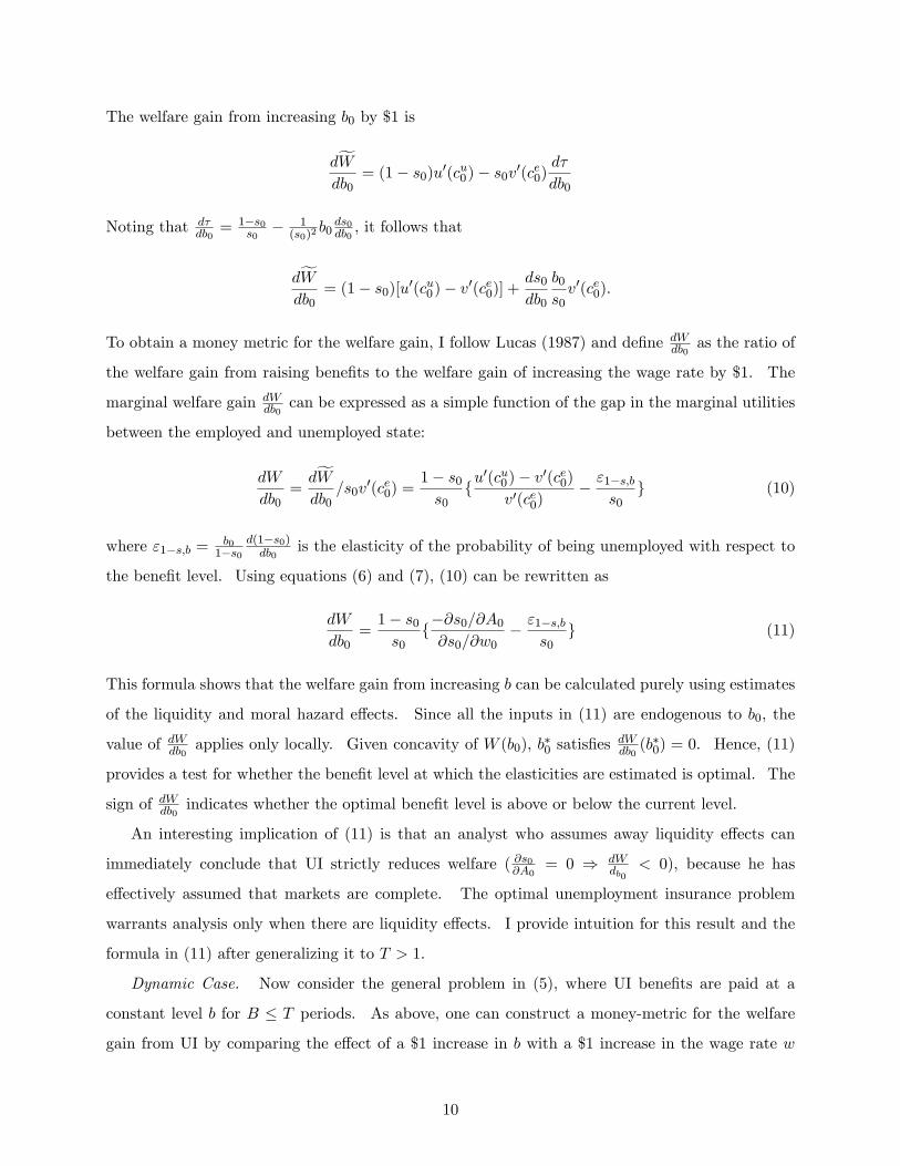
The welfare gain from increasing b0 by $1 is

dfWdb0

= (1� s0)u0(cu0)� s0v0(ce0)d�

db0

Noting that d�db0= 1�s0

s0� 1

(s0)2b0ds0db0, it follows that

dfWdb0

= (1� s0)[u0(cu0)� v0(ce0)] +ds0db0

b0s0v0(ce0).

To obtain a money metric for the welfare gain, I follow Lucas (1987) and de�ne dWdb0

as the ratio of

the welfare gain from raising bene�ts to the welfare gain of increasing the wage rate by $1. The

marginal welfare gain dWdb0

can be expressed as a simple function of the gap in the marginal utilities

between the employed and unemployed state:

dW

db0=dfWdb0

=s0v0(ce0) =

1� s0s0

fu0(cu0)� v0(ce0)

v0(ce0)� "1�s;b

s0g (10)

where "1�s;b =b01�s0

d(1�s0)db0

is the elasticity of the probability of being unemployed with respect to

the bene�t level. Using equations (6) and (7), (10) can be rewritten as

dW

db0=1� s0s0

f�@s0=@A0@s0=@w0

� "1�s;bs0

g (11)

This formula shows that the welfare gain from increasing b can be calculated purely using estimates

of the liquidity and moral hazard e¤ects. Since all the inputs in (11) are endogenous to b0, the

value of dWdb0 applies only locally. Given concavity of W (b0), b�0 satis�es

dWdb0(b�0) = 0. Hence, (11)

provides a test for whether the bene�t level at which the elasticities are estimated is optimal. The

sign of dWdb0 indicates whether the optimal bene�t level is above or below the current level.

An interesting implication of (11) is that an analyst who assumes away liquidity e¤ects can

immediately conclude that UI strictly reduces welfare ( @s0@A0= 0 ) dW

db0< 0), because he has

e¤ectively assumed that markets are complete. The optimal unemployment insurance problem

warrants analysis only when there are liquidity e¤ects. I provide intuition for this result and the

formula in (11) after generalizing it to T > 1.

Dynamic Case. Now consider the general problem in (5), where UI bene�ts are paid at a

constant level b for B � T periods. As above, one can construct a money-metric for the welfare

gain from UI by comparing the e¤ect of a $1 increase in b with a $1 increase in the wage rate w

10

on the agent�s expected utility: dWdb �

dJ0db =

T�1Pt=0

dJ0dwt. Let � = T�D

T denote the fraction of his life

the agent is employed. Let "DB ;b =bDB

dDBdb and "D;b = b

DdDdb denote the total elasticities of the

UI-compensated and total unemployment duration with respect to the UI bene�t level, taking into

account the e¤ect of the increase in � needed to �nance the increase in b.

When T > 1, the e¤ects of bene�t and tax increases on welfare depend on the entire path of

marginal utilities after re-employment. In addition, when B < T , dWdb depends on both DB and

D. These factors make the formula for dWdb more complex, as shown in the following proposition.

Proposition 1 Suppose UI bene�ts are paid for B periods at a level b. The welfare gain from

raising b by $1 relative to a $1 increase in the wage is:

dW

db(b) =

1� ��

DBDf(1� �)

�@s0@a jB

@s0@w jB

� �� 1

�((1� �)"D;b + �"DB ;b)g. (12)

where � = E0;B�1v0(cet )�v0(ce0)E0;T�1v0(cet )

BDB+E0;B�1v0(cet )�E0;T�1v0(cet )

E0;T�1v0(cet )and E0;sv0(cet ) denotes the average marginal

utility of consumption after re-employment conditional on �nding a job before period s.

Proof. The general logic of the proof is to write the welfare gain in terms of marginal utilities,

as in (10), and then relate these marginal utilities to the moral hazard and liquidity comparative

statics. See Appendix A for details.

The formula for dWdb when T � B > 1 di¤ers from the formula in (11) for the static case in three

respects. First, the welfare gain depends on a new parameter � in addition to the liquidity and

moral hazard e¤ects. The parameter � is an increasing function of the sensitivity of consumption

upon re-employment to the length of the preceding unemployment spell, i.e. the rate at which v0(cet )

rises with t. The � term enters the formula because part of the liquidity e¤ect arises from the

di¤erence in expected marginal utilities after re-employment at di¤erent dates when T > 1. This

component of the liquidity e¤ect has to be subtracted out, because only the di¤erence in marginal

utilities between the employed and unemployed states matters for optimal UI.

Second, when B < T , dWdb depends on a weighted average of "D;b and "DB ;b because

d�db is

determined by both the time the agent spends on the UI system and the time he spends working

and paying taxes. Third, the welfare gain is scaled down by DBD < 1 because UI bene�ts are paid

for only a fraction DBD of the unemployment spell, reducing the welfare gain from raising b relative

to the welfare gain of a permanent wage increase.

11

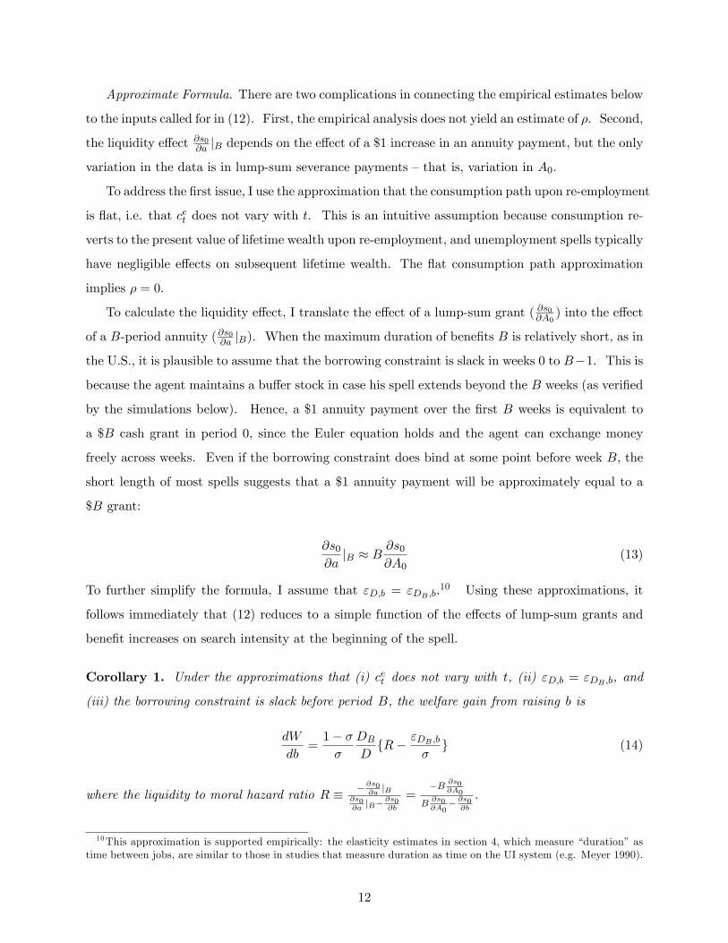
Approximate Formula. There are two complications in connecting the empirical estimates below

to the inputs called for in (12). First, the empirical analysis does not yield an estimate of �. Second,

the liquidity e¤ect @s0@a jB depends on the e¤ect of a $1 increase in an annuity payment, but the only

variation in the data is in lump-sum severance payments �that is, variation in A0.

To address the �rst issue, I use the approximation that the consumption path upon re-employment

is �at, i.e. that cet does not vary with t. This is an intuitive assumption because consumption re-

verts to the present value of lifetime wealth upon re-employment, and unemployment spells typically

have negligible e¤ects on subsequent lifetime wealth. The �at consumption path approximation

implies � = 0.

To calculate the liquidity e¤ect, I translate the e¤ect of a lump-sum grant ( @s0@A0) into the e¤ect

of a B-period annuity (@s0@a jB). When the maximum duration of bene�ts B is relatively short, as in

the U.S., it is plausible to assume that the borrowing constraint is slack in weeks 0 to B�1. This is

because the agent maintains a bu¤er stock in case his spell extends beyond the B weeks (as veri�ed

by the simulations below). Hence, a $1 annuity payment over the �rst B weeks is equivalent to

a $B cash grant in period 0, since the Euler equation holds and the agent can exchange money

freely across weeks. Even if the borrowing constraint does bind at some point before week B, the

short length of most spells suggests that a $1 annuity payment will be approximately equal to a

$B grant:

@s0@ajB � B

@s0@A0

(13)

To further simplify the formula, I assume that "D;b = "DB ;b.10 Using these approximations, it

follows immediately that (12) reduces to a simple function of the e¤ects of lump-sum grants and

bene�t increases on search intensity at the beginning of the spell.

Corollary 1. Under the approximations that (i) cet does not vary with t, (ii) "D;b = "DB ;b, and

(iii) the borrowing constraint is slack before period B, the welfare gain from raising b is

dW

db=1� ��

DBDfR� "DB ;b

�g (14)

where the liquidity to moral hazard ratio R � � @s0@ajB

@s0@ajB�

@s0@b

=�B @s0

@A0

B@s0@A0

� @s0@b

.

10This approximation is supported empirically: the elasticity estimates in section 4, which measure �duration�astime between jobs, are similar to those in studies that measure duration as time on the UI system (e.g. Meyer 1990).

12

Quality of Approximations. How accurate of an approximation does (14) provide for the actual

welfare gain? I answer this question by comparing the actual (numerically calculated) and approx-

imate welfare gains from raising the bene�t level using simulations with the same parametrization

as in section 2.2 and A0 = 100. I compute the actual welfare gain by calculating J0(b; w) numer-

ically and de�ning @W@b =

J0(b+1)�J0(b)J0(w+1)�J0(w) . I compute the approximate welfare gain by calculating

@s0=@A0, @s0=@b, and "DB ;b numerically and applying the formula in Corollary 1.

Figure 2 plots the actual and approximate values of dWdb as a function of the wage replacement

rate bw . The �gure shows, for instance, that the welfare gain of raising the UI bene�t level by $1

starting from a replacement rate of 50% is equivalent to a permanent 3.5 cent wage increase. The

welfare gain falls with b because J0 is concave in b �there are diminishing returns to correcting

market failures. The approximate welfare gain is very similar to the actual welfare gain, with

an average deviation of 0.2 cents over the range plotted. At all but the lowest replacement rates

( bw < 15%), the approximate and actual measures are indistinguishable. The similarity is striking

given how much less information is used to implement the approximate formula than the actual

(�structural approach�) measure.

The approximation works well for two reasons. First, the consumption path upon re-employment

fcetg is quite �at; for example, when b = 0:5w, ce0 = $423:50 and ce26 = $423:46. As a result, � is

close to 0 (� = �0:002).11 Second, the borrowing constraint is slack for t < 26 when bw > 15%.

Since bene�ts are provided for only 26 weeks, the agent retains a bu¤er stock to insure against the

risk of a spell beyond 26 weeks. For instance, when b = 0:5, the agent enters week 26 with $75 in

assets if he is still unemployed at that time, even though he could have borrowed up to $1000. The

annuity to cash grant conversion in (13) therefore holds exactly for b > 0:15w. When b < 0:15w,

the borrowing constraint starts to bind in the fourth or �fth month, leading to a modest error in

the annuity conversion because most spells end before this point.12

The welfare gain remains positive even at b = 0:95w because of the stylized nature of the

simulation. Allowing for private-market or informal insurance mechanisms would substantially

reduce the simulated welfare gains, particularly at high bene�t levels. This sensitivity to modelling

assumptions is precisely the advantage of using the elasticity-based formula in (14) rather than

simulating the welfare gains from the structural model, as I discuss below.

11 In this numerical example, fcetg is particularly �at because the agent does not borrow against future earningswhile unemployed prior to week B = 26 because of the risk that the spell may extend beyond the UI exhaustion date.In the appendix, I give a bounding argument showing that � < 0:015 irrespective of the agent�s borrowing decisions.12 If @s0

@ajB were empirically estimable, the approximate measure would remain equally accurate for b

w< 15%.

Hence, the only potentially non-trivial source of approximation error is the annuity conversion in (13).

13

2.4 Extensions

Endogenous Ex-Ante Behavior. The preceding welfare analysis assumed that behavior prior to

job loss is invariant to the unemployment bene�t level. In practice, higher bene�ts might reduce

precautionary saving and private market insurance arrangements. To understand how such ex-ante

behavioral responses a¤ect Corollary 1, suppose the agent is employed at wage w�1 � � in period

t = �1. He faces a (�xed) probability p of being laid o¤ in period 0, at which point the problem

speci�ed in section 2.1 begins. With probability 1 � p, the agent is granted tenure and remains

employed until T . The agent can purchase an insurance policy that pays $z if he is laid o¤ and

charges a premium !(z) if he remains employed.13 The agent�s value function in period �1 is:

J�1(A�1) = maxA0;z

v(w�1 � � �A0) + pJ0(A0 + z) + (1� p)Tv(wt � � +A0 � !(z)

T) (15)

The social planner�s problem is to

maxb;�

J�1(b; �) s.t. pDBb = (T + 1� pD)� (16)

Let us rede�ne dWdb � dJ�1

db =T�1Pt=�1

dJ�1dwt

and the fraction of time employed as � = T+1�pDT+1 . In

Appendix A, I show that Corollary 1 remains valid in this extended model subject to one caveat:

the derivatives @s0@a jB and

@s0@b must be evaluated holding the ex-ante choices of A0 and z �xed.

14

Intuitively, endogenous ex-ante behaviors have no e¤ect on the marginal utility representation in

(10) because of envelope conditions that eliminate �rst-order e¤ects of these behavioral responses.

The liquidity and moral hazard comparative statics, however, are confounded by changes in ex-

ante behavior, breaking the link between the ratio R and the gap in marginal utilities between

the employed and unemployed states. Conditioning on A0 and z when calculating the derivatives

restores the link between @s0@a jB=

@s0@b and the gap in marginal utilities.

Thus, (14) holds with endogenous ex-ante behavior, but the variation used to estimate the

liquidity and moral hazard e¤ects must be chosen judiciously. In the empirical application below,

@s0@b is estimated from unanticipated changes in bene�t rules, making it plausible that ex-ante

13There is still a potential role for government-provided insurance in this model because private insurance mayhave a load (!(z) > p

1�pz). Note that the private insurance policy considered here does not induce moral hazardbecause it does not a¤ect the marginal incentive to search. Allowing for private insurance policies that induce moralhazard requires a modi�cation of the formula because of a �scal externality problem. See Chetty and Saez (2008)for an extension of the formula in (14) to this case.14 If @s0

@ajB is estimated using variation in severance payments and the annuity conversion in (13), the e¤ect of

severance pay on durations must be estimated holding savings behavior prior to job loss �xed.

14

behaviors are una¤ected by the variation in b. In other contexts, such as cross-sectional comparisons

of unemployment durations across states or countries, ex-ante behavioral responses may a¤ect the

elasticities.

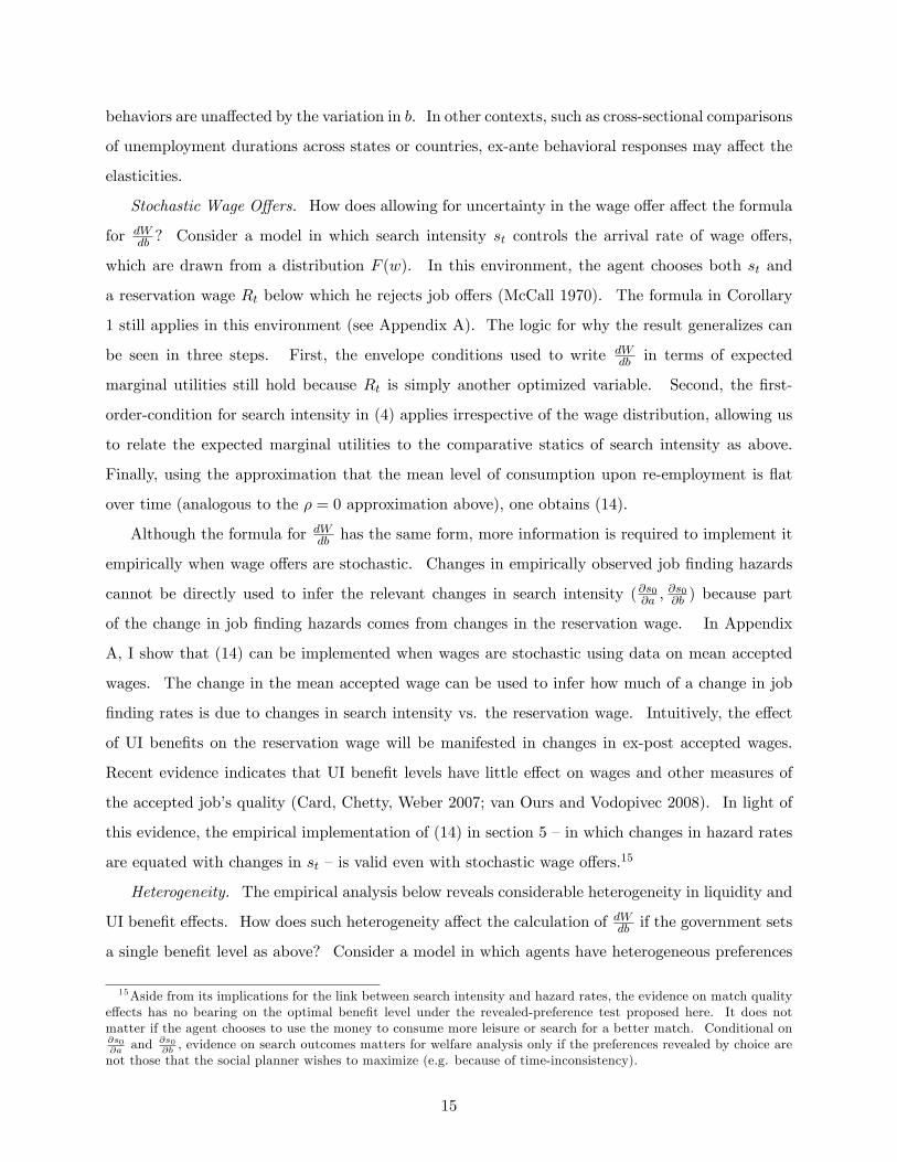
Stochastic Wage O¤ers. How does allowing for uncertainty in the wage o¤er a¤ect the formula

for dWdb ? Consider a model in which search intensity st controls the arrival rate of wage o¤ers,

which are drawn from a distribution F (w). In this environment, the agent chooses both st and

a reservation wage Rt below which he rejects job o¤ers (McCall 1970). The formula in Corollary

1 still applies in this environment (see Appendix A). The logic for why the result generalizes can

be seen in three steps. First, the envelope conditions used to write dWdb in terms of expected

marginal utilities still hold because Rt is simply another optimized variable. Second, the �rst-

order-condition for search intensity in (4) applies irrespective of the wage distribution, allowing us

to relate the expected marginal utilities to the comparative statics of search intensity as above.

Finally, using the approximation that the mean level of consumption upon re-employment is �at

over time (analogous to the � = 0 approximation above), one obtains (14).

Although the formula for dWdb has the same form, more information is required to implement it

empirically when wage o¤ers are stochastic. Changes in empirically observed job �nding hazards

cannot be directly used to infer the relevant changes in search intensity (@s0@a ;@s0@b ) because part

of the change in job �nding hazards comes from changes in the reservation wage. In Appendix

A, I show that (14) can be implemented when wages are stochastic using data on mean accepted

wages. The change in the mean accepted wage can be used to infer how much of a change in job

�nding rates is due to changes in search intensity vs. the reservation wage. Intuitively, the e¤ect

of UI bene�ts on the reservation wage will be manifested in changes in ex-post accepted wages.

Recent evidence indicates that UI bene�t levels have little e¤ect on wages and other measures of

the accepted job�s quality (Card, Chetty, Weber 2007; van Ours and Vodopivec 2008). In light of

this evidence, the empirical implementation of (14) in section 5 �in which changes in hazard rates

are equated with changes in st �is valid even with stochastic wage o¤ers.15

Heterogeneity. The empirical analysis below reveals considerable heterogeneity in liquidity and

UI bene�t e¤ects. How does such heterogeneity a¤ect the calculation of dWdb if the government sets

a single bene�t level as above? Consider a model in which agents have heterogeneous preferences

15Aside from its implications for the link between search intensity and hazard rates, the evidence on match qualitye¤ects has no bearing on the optimal bene�t level under the revealed-preference test proposed here. It does notmatter if the agent chooses to use the money to consume more leisure or search for a better match. Conditional on@s0@a

and @s0@b, evidence on search outcomes matters for welfare analysis only if the preferences revealed by choice are

not those that the social planner wishes to maximize (e.g. because of time-inconsistency).

15

and asset levels and the government has a utilitarian social welfare function. De�ne dWdb as the

aggregate marginal welfare gain from raising b relative to raising the wage rate for all agents. Then

dWdb has the same representation as in (10), replacing the marginal utilities by average marginal

utilities across agents (see Appendix A). However, connecting the gap in average marginal utilities

to the ratio of the mean liquidity and moral hazard e¤ects (R =�B�E @s0

@A

E @s0@b

) requires additional

assumptions. This is because agents with high values of 00(s0) receive less weight in both the

mean liquidity and moral hazard e¤ects since their behavior is less elastic to policy changes. But

all agents receive equal weight in the welfare calculation under the utilitarian criterion. If the

heterogeneity in marginal utilities (v0(cet ); u0(cet )) is orthogonal to the heterogeneity in

00(s0) �that

is, if the parameters which control heterogeneity in preferences over consumption and disutility of

search are independently distributed �the 00(s0) terms cancel out of R. Under this independence

assumption, the formula for dWdb in Corollary 1 measures the mean per-capita welfare gain of raising

b when calibrated using mean e¤ects as in section 5.

2.5 Discussion

Intuition for the Test. The analysis above has shown that the optimal bene�t level does not

necessarily fall with "D;b, contrary to conventional wisdom. It matters whether a higher value of

"D;b comes from a larger liquidity (�@s0@a jB) or moral hazard (

@s0@w jB) component. To the extent

that it is the liquidity e¤ect, UI reduces the need for agents to rush back to work because they

have insu¢ cient ability to smooth consumption; if it is primarily the moral hazard e¤ect, UI is

subsidizing unproductive leisure. In this sense, the formula for optimal UI proposed here can be

interpreted as a new method of quantifying the extent to which the full insurance benchmark is

violated. The agent�s capacity to smooth marginal utilities is assessed by examining the e¤ect

of transitory income shocks on the consumption of leisure instead of goods as in earlier studies

(Cochrane 1991, Gruber 1997).

More generally, the concept underlying (14) is to measure the value of insurance using revealed

preference. The e¤ect of a lump-sum cash grant on the unemployment duration reveals the extent

to which the UI bene�t permits the agent to attain a more socially desirable allocation. If a

lump-sum grant has no e¤ect on the duration of search, we infer that the agent is taking more time

to �nd a job when the UI bene�t level is increased purely because of the price subsidy for doing so.

In this case, UI simply creates ine¢ ciency by taxing work, and dWdb < 0. In contrast, if the agent

raises his duration substantially even when he receives a non-distortionary cash grant, we infer that

16

the UI bene�t permits him to make a more (socially) optimal choice, i.e. the choice he would make

if the credit and insurance market failures could be alleviated without distorting incentives. The

test thus identi�es the policy that is best from the libertarian criterion of correcting market failures

as revealed by individual choice.

Comparison to Alternative Methods. The most widely used existing method of policy analysis is

the structural approach, which involves two steps: �rst, estimate the primitives using a parametrized

model of behavior �e.g. the curvature of the utility function, the cost of search e¤ort, the borrowing

limit, etc. Second, simulate the e¤ect of policy changes using the estimated model, as in the

calculation of the actual welfare gain in Figure 2. Wolpin (1987) pioneered the application of this

approach to job search; more recent examples include Hansen and Imrohoglu (1992), Hopenhayn

and Nicolini (1997), and Lentz (2008).

In contrast with the structural approach, the formula in Corollary 1 leaves the primitives uniden-

ti�ed. It instead identi�es a set of high-level moments ("DB ;b, R, DB) that are su¢ cient statistics

for the marginal value of insurance (up to the approximations necessitated by data limitations).

The primitives do not need to be identi�ed because any combination of primitives that matches

("DB ;b, R, DB) at a given level of b implies the same value ofdWdb (b). For example, any primitives

consistent with these three moments at b = 0:5w in Figure 2 would lead to dWdb (b = 0:5w) = 0:035.

Changes in the primitives a¤ect the marginal welfare gain only through these three moments be-

cause of envelope conditions that arise from agent optimization (see also Chetty 2006a). Thus, the

three moments exactly identify the welfare gain from UI.

The same concept of exact identi�cation underlies the consumption-based formula for optimal

UI bene�ts of Baily (1978) and Chetty (2006a) and the reservation-wage formula of Shimer and

Werning (2007). Each of these papers identi�es a di¤erent su¢ cient statistic for welfare analysis.

One advantage of the moral hazard vs. liquidity method is that it requires data only on unemploy-

ment durations, which are typically more precise and widely available than data on consumption

or reservation wages. In addition, this method does not rely on consumption-labor separability

(u = v) or a speci�c parametrization of the utility function, and can be easily implemented when

bene�ts have �nite duration (B < T ).16

The general advantage of exact identi�cation methods relative to the structural approach is

that they require much less information about preferences and technology. For instance, (14) is

16The formula here does, however, assume separability of utility over consumption and search e¤ort in the un-employed state. Complementarities between ct and st can be handled by estimating the cross-partial using thetechnique in Chetty (2006b).

17

invariant to assumptions about market completeness, as measured by the asset limit L and the cost

of private insurance !(z). Structural approaches, in contrast, often require assumptions such as

no intertemporal smoothing or no private insurance to operationalize the analysis. Moreover, even

granted such assumptions, it is challenging to identify every primitive consistently in view of model

mis-speci�cation and omitted variable concerns. A biased estimate of any one of the structural

primitives creates bias in the welfare analysis. Since it is easier to estimate a small set of elasticities

using credible identi�cation strategies, exact identi�cation is likely to yield more empirically and

theoretically robust welfare conclusions.

The disadvantage of (existing) exact identi�cation strategies is the limited scope of questions

that they can answer. One cannot, for example, make statements about the welfare gain from an

inde�nite (B = T ) UI bene�t using the method develop above when the variation in the data is

only in �nite duration (B < T ) policies. In addition, because the elasticity inputs to the formula

are endogenous to the policy itself, exact identi�cation can only be used to calculate marginal

welfare e¤ects �that is, the e¤ect of local changes in policy around observed values. Structural

methods, in contrast, can in principle be used to simulate the welfare e¤ect of any policy change

once the primitives have been estimated, since the primitives are by de�nition exogenous to policy

changes.17

In the remainder of the paper, I calculate the welfare gain from raising the UI bene�t level in

the U.S. by estimating @s0@b and

@s0@A0

. I compare the results of this method with results of other

approaches in the existing literature in section 5.

3 Empirical Analysis I: The Role of Constraints

3.1 Estimation Strategy

The objective of the empirical analysis is to estimate the liquidity and total bene�t e¤ects for

liquidity-constrained and unconstrained households. The empirical strategy follows from the pos-

itive analysis in section 2.2; I essentially estimate the slope of the four curves simulated in Figure

1. I begin by comparing the e¤ect of UI bene�ts on durations for unconstrained and constrained

individuals. This comparison gives an indication of the importance of liquidity relative to moral

hazard. For instance, if the e¤ects of bene�ts on durations were much stronger in the unconstrained

17 In practice, structural estimation generally relies on out-of-sample parametric extrapolations to make statementsabout policies outside the region observed in the data. Using such extrapolations, one could potentially extend theexact identi�cation welfare results outside the observed region as well.

18

group, it would be unlikely that liquidity e¤ects are large.

To implement this heterogeneity analysis, I divide individuals into unconstrained and con-

strained groups and estimate bene�t-duration elasticities for each group using cross-state and time

variation in unemployment bene�t levels. The ideal de�nition of the unconstrained group would

be the set of households whose marginal utility is not sensitive to transitory income shocks �i.e.,

those who have � = u0(cut ) � v0(cet ) ' 0. Unfortunately, there is no panel dataset that contains

high-frequency information on both household consumption and labor supply in the U.S. I there-

fore use proxies to identify households that can smooth consumption intertemporally, who should

have � ' 0 as shown in the simulations above.18

The primary proxy I use is liquid wealth net of unsecured debt at the time of job loss, which

I term �net wealth.� Browning and Crossley (2001), Bloemen and Stancanelli (2005), and Sulli-

van (2007) report evidence from various panel datasets showing that households with little or no

�nancial assets prior to job loss su¤er consumption drops during unemployment that are mitigated

by provision of UI bene�ts. In contrast, households with higher assets exhibit little sensitivity of

consumption to unemployment or UI bene�t levels.19

I also consider two secondary proxies: spousal work status and mortgage status prior to job

loss. Browning and Crossley �nd larger consumption drops and higher sensitivity to UI among

single-earner households. Their interpretation of this �nding is that those with a second income

source are more likely to be able to borrow since at least one person is employed.20 The mortgage

proxy is motivated by Gruber�s (1998) �nding that fewer than 5% of the unemployed sell their

homes during a spell, whereas renters move much more frequently. Consequently, an individual

making mortgage payments before job loss e¤ectively has less ability to smooth the remainder of

his consumption (Chetty and Szeidl 2007), and is more likely to be constrained than a renter.

Although these proxies predict being constrained on average, they are imperfect predictors for

two reasons. First, some households classi�ed as unconstrained are presumably misallocated to

the constrained group and vice-versa. Second, no household truly has � = 0 because insurance

markets are likely to be incomplete. There is therefore a small liquidity e¤ect even among the

18An alternative strategy, which I do not pursue here because of data limitations, is to distinguish households bytheir ability to smooth consumption across states through risk-sharing mechanisms.19Related evidence is given by Blundell, Pistaferri, and Preston (2008), who �nd that consumption-income co-

movement is much larger for low-asset households.20A countervailing e¤ect is that households with a single earner may be able to maintain their prior standard of

living more easily if the other earner can enter the labor force to make up for the lost income. Browning and Crossley�s�ndings suggest that this e¤ect is dominated by the added intertemporal smoothing capacity of dual earners, so thaton net households with two earners are less constrained.

19

groups classi�ed as unconstrained, as shown in Figure 1. Since I attribute the entire response

among the group classi�ed as unconstrained to moral hazard, both of these misclassi�cation errors

lead to underestimation of the liquidity e¤ect relative to moral hazard.

3.2 Data

I use data from the Survey of Income and Program Participation (SIPP) panels spanning 1985-

2000. Each SIPP panel surveys households at four month intervals for 2-4 years. Relative to other

widely used datasets such as the CPS and PSID, the main bene�ts of the SIPP are the availability

of asset data, weekly data on employment status, data on UI bene�t receipt, and large sample size.

Starting from the universe of job separations in the pooled SIPP panels, I restrict attention to

prime-age males who (a) report searching for a job, (b) are not on temporary layo¤, (c) have at least

three months of work history in the survey (so that pre-unemployment wages can be computed),

and (d) took up UI bene�ts within one month after job loss.21 Details on the sample construction

and SIPP database are given in Appendix B. The restrictions leave 4,560 unemployment spells

in the core analysis sample. Asset data are generally collected only once in each panel, so pre-

unemployment asset data is available for approximately half of these observations.

The �rst column of Table 1 gives summary statistics for the core sample. Monetary values are

in real 1990 dollars in this and all subsequent tables. The median UI recipient is a high school

graduate and has pre-UI gross annual earnings of $20,711. Perhaps the most striking statistic is

pre-unemployment wealth: median liquid wealth net of unsecured debt is only $128, suggesting that

many unemployed individuals may not be in a position to smooth consumption while unemployed.

Information on UI laws was obtained from the Employment and Training Administration (var-

ious years) and supplemented with information directly from individual states. Unfortunately,

measurement error and inadequate information about pre-unemployment wages for many claimants

make it di¢ cult to predict each claimant�s bene�t level precisely. I therefore use three independent

methods to proxy for each claimant�s (unobserved) actual UI bene�ts. First, I use average bene�ts

for each state/year pair obtained from the Department of Labor in lieu of each individual�s actual

UI bene�t amount. Second, I proxy for the actual bene�t using maximum weekly bene�t amounts,

which are the primary source of variation in bene�t levels across states, since most states replace

21Restricting the sample to those who take up UI could lead to selection bias because the takeup decision isendogenous to the bene�t level (Anderson and Meyer 1997). I �nd that the elasticity of takeup with respect to thebene�t level is similar across the constrained and unconstrained groups, suggesting that endogeneity is unlikely to beresponsible for the heterogeneous e¤ects estimated below.

20

50% of a claimant�s wages up to a maximum bene�t level. Third, I simulate each individual�s

weekly UI bene�t using a two-stage procedure. In the �rst stage, I predict each claimant�s pre-

unemployment annual income using education, age, occupation, and other demographics. In the

second stage, I predict each claimant�s unemployment bene�ts using a simulation program that as-

signs each claimant a bene�t based on the predicted wage, state, and year of claim. See Appendix

B for further details on the motivation for and implementation of this two-stage procedure.

3.3 Results

3.3.1 Graphical Evidence and Non-Parametric Tests

I begin by providing graphical evidence on the e¤ect of unemployment bene�ts on durations in

constrained and unconstrained groups. First consider the asset proxy for constraints. I divide

households into four quartiles based on their net liquid wealth. Table 1 shows summary statistics

for each of the four quartiles. Households in the lower net liquid wealth quartiles are poorer and

less educated, but the di¤erences between the four groups are not very large. As a result, UI

bene�t levels are fairly constant across the groups. In particular, the replacement rate �de�ned

as each individual�s simulated unemployment bene�t divided by his predicted wage � is close to

50% on average in all four quartiles. This similarity of bene�t and income levels suggests that

di¤erences in bene�t-duration elasticities across the quartiles are unlikely to be driven purely by

di¤erences in the levels around which the elasticities are estimated.

Figures 3a-d show the e¤ect of UI bene�ts on job-�nding rates for households in the each of the

four quartiles of the net wealth distribution. Since ex-post asset levels are endogenous to duration

of unemployment, households for whom asset data are available only after job loss are excluded

when constructing these �gures. Including these households turns out to have little e¤ect on the

results, as we will see below in the regression analysis. I construct the �gures by �rst dividing

the full sample of UI claimants into two categories: those that are in (state, year) pairs that have

average weekly bene�t amounts above the sample median and those below the median. I then plot

Kaplan-Meier survival curves for these two groups using the households in the relevant net wealth

quartile. Note that the di¤erences in average individual replacement rates between the low and

high-bene�t are fairly similar in the four quartiles.

These and all subsequent survival curves plotted using the SIPP data are adjusted for the �seam

e¤ect�in panel surveys. Individuals are interviewed at 4 month intervals in the SIPP and tend to

repeat answers about weekly job status in the past four months. Consequently, a disproportionately

21

large number of transitions in labor force status are reported on the �seam�between interviews,

leading to arti�cial spikes in the hazard rate at 4 and 8 months. These spikes are smoothed out by

�tting a Cox model with a time-varying indicator for being on a seam between interviews, and then

recovering the baseline hazards to construct a seam-adjusted Kaplan-Meier curve. The resulting

survival curves give the probability of remaining unemployed after t weeks for an individual who

never crosses an interview seam. The results are similar if the raw data is used without adjusting

for the seam e¤ect.

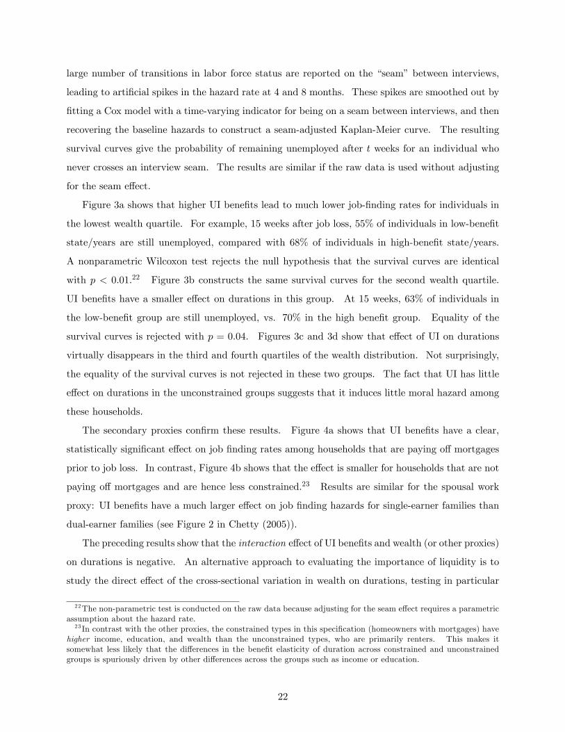
Figure 3a shows that higher UI bene�ts lead to much lower job-�nding rates for individuals in

the lowest wealth quartile. For example, 15 weeks after job loss, 55% of individuals in low-bene�t

state/years are still unemployed, compared with 68% of individuals in high-bene�t state/years.

A nonparametric Wilcoxon test rejects the null hypothesis that the survival curves are identical

with p < 0:01.22 Figure 3b constructs the same survival curves for the second wealth quartile.

UI bene�ts have a smaller e¤ect on durations in this group. At 15 weeks, 63% of individuals in

the low-bene�t group are still unemployed, vs. 70% in the high bene�t group. Equality of the

survival curves is rejected with p = 0:04. Figures 3c and 3d show that e¤ect of UI on durations

virtually disappears in the third and fourth quartiles of the wealth distribution. Not surprisingly,

the equality of the survival curves is not rejected in these two groups. The fact that UI has little

e¤ect on durations in the unconstrained groups suggests that it induces little moral hazard among

these households.

The secondary proxies con�rm these results. Figure 4a shows that UI bene�ts have a clear,

statistically signi�cant e¤ect on job �nding rates among households that are paying o¤ mortgages

prior to job loss. In contrast, Figure 4b shows that the e¤ect is smaller for households that are not

paying o¤ mortgages and are hence less constrained.23 Results are similar for the spousal work

proxy: UI bene�ts have a much larger e¤ect on job �nding hazards for single-earner families than

dual-earner families (see Figure 2 in Chetty (2005)).

The preceding results show that the interaction e¤ect of UI bene�ts and wealth (or other proxies)

on durations is negative. An alternative approach to evaluating the importance of liquidity is to

study the direct e¤ect of the cross-sectional variation in wealth on durations, testing in particular

22The non-parametric test is conducted on the raw data because adjusting for the seam e¤ect requires a parametricassumption about the hazard rate.23 In contrast with the other proxies, the constrained types in this speci�cation (homeowners with mortgages) have

higher income, education, and wealth than the unconstrained types, who are primarily renters. This makes itsomewhat less likely that the di¤erences in the bene�t elasticity of duration across constrained and unconstrainedgroups is spuriously driven by other di¤erences across the groups such as income or education.

22

if durations are an increasing and concave function of wealth. I focus on the variation in UI

bene�ts because changes in UI laws are credibly exogenous to individuals�preferences. In contrast,

conditional on demographics and income, cross-sectional variation in wealth holdings arises from

heterogeneity in tastes for savings, confounding the e¤ect of wealth on duration in the cross-section.

For example, UI claimants with higher assets are also likely to have lower discount rates or higher

anticipated expenses (e.g., college tuition payments), and hence may be reluctant to deplete their

assets to �nance a longer spell of unemployment.24 In practice, I �nd no robust relationship between

assets and unemployment durations in the cross-section (as indicated by the mean durations by

quartile reported in Table 1), consistent with the results of Lentz (2007). This �nding underscores

the importance of using exogenous variation such as UI bene�ts for identi�cation. The same issue

also motivates the use of severance pay as a source of variation in wealth to identify the liquidity

e¤ect in section 4.

3.3.2 Hazard Model Estimates

I evaluate the robustness of the graphical results by estimating a set of Cox hazard models in Table

2. Let hi;t denote the unemployment exit hazard rate for individual i in week t of an unemployment

spell, �t the �baseline�hazard rate in week t, bi the unemployment bene�t level for individual i,

and Xi;t a set of controls. Throughout, I censor durations at 50 weeks to reduce the in�uence of

outliers and focus on search behavior in the year after job loss.

Since the welfare gain formula (14) calls for estimates of the e¤ect of UI bene�ts on search

behavior at the beginning of the spell (@s0=@b), I estimate hazard models of the following form:

log hi;t = �t + �1 log bi + �2t� log bi + �3Xi;t (17)

Here, the coe¢ cient �1 gives the elasticity of the hazard rate with respect to UI bene�ts at the

beginning of the spell (t = 0) because the interaction term t� log bi captures any time-varying e¤ect

of UI bene�ts on hazards. Note that the search model does not make a clear prediction about the

sign of �2. The e¤ect of UI bene�ts could diminish over time (�2 < 0) because the number of weeks

for which bene�ts remain available is falling. But �2 could also be positive because households

are increasingly constrained and thus more sensitive to cash-on-hand late in the spell. In practice,

there is no robust, statistically signi�cant pattern in the �2 coe¢ cients across the quartiles, and I

24More generally, wealthier individuals may have unobserved characteristics (e.g. skills, job search technologies)that lead to di¤erent durations for reasons unrelated to their wealth.

23

therefore do not report them in Table 2 in the interest of space.25

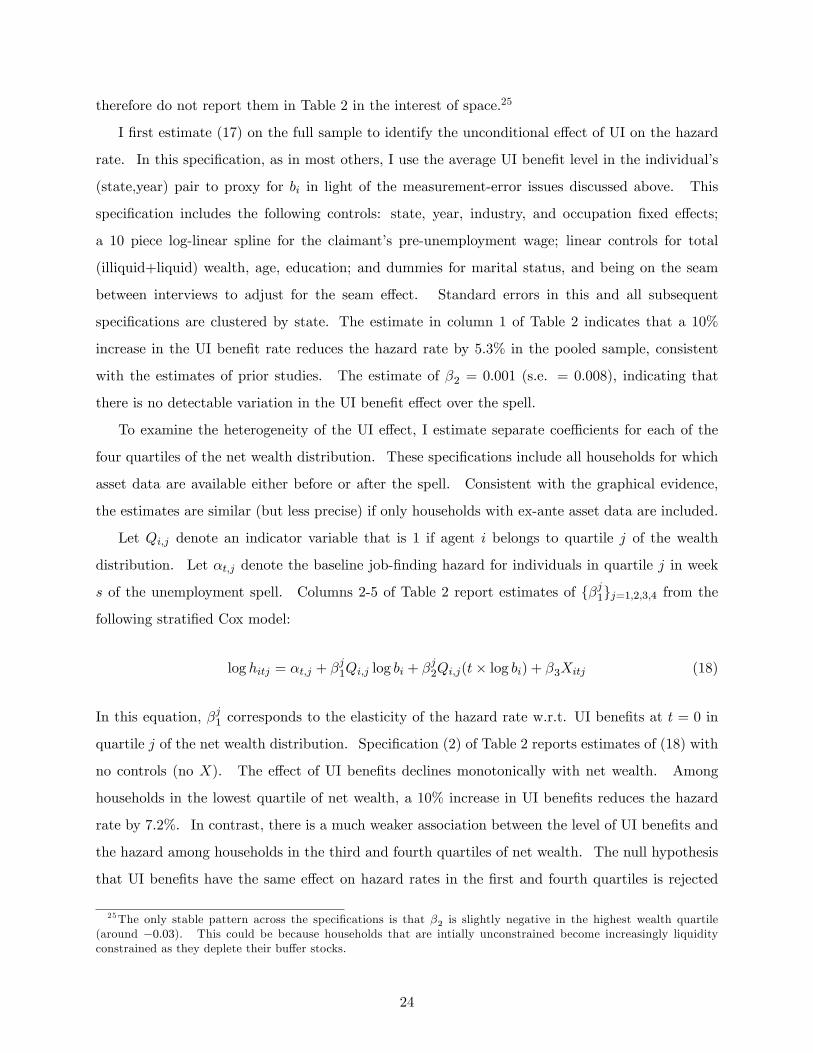
I �rst estimate (17) on the full sample to identify the unconditional e¤ect of UI on the hazard

rate. In this speci�cation, as in most others, I use the average UI bene�t level in the individual�s

(state,year) pair to proxy for bi in light of the measurement-error issues discussed above. This

speci�cation includes the following controls: state, year, industry, and occupation �xed e¤ects;

a 10 piece log-linear spline for the claimant�s pre-unemployment wage; linear controls for total

(illiquid+liquid) wealth, age, education; and dummies for marital status, and being on the seam

between interviews to adjust for the seam e¤ect. Standard errors in this and all subsequent

speci�cations are clustered by state. The estimate in column 1 of Table 2 indicates that a 10%

increase in the UI bene�t rate reduces the hazard rate by 5.3% in the pooled sample, consistent

with the estimates of prior studies. The estimate of �2 = 0:001 (s.e. = 0:008), indicating that

there is no detectable variation in the UI bene�t e¤ect over the spell.

To examine the heterogeneity of the UI e¤ect, I estimate separate coe¢ cients for each of the

four quartiles of the net wealth distribution. These speci�cations include all households for which

asset data are available either before or after the spell. Consistent with the graphical evidence,

the estimates are similar (but less precise) if only households with ex-ante asset data are included.

Let Qi;j denote an indicator variable that is 1 if agent i belongs to quartile j of the wealth

distribution. Let �t;j denote the baseline job-�nding hazard for individuals in quartile j in week

s of the unemployment spell. Columns 2-5 of Table 2 report estimates of f�j1gj=1;2;3;4 from the

following strati�ed Cox model:

log hitj = �t;j + �j1Qi;j log bi + �

j2Qi;j(t� log bi) + �3Xitj (18)

In this equation, �j1 corresponds to the elasticity of the hazard rate w.r.t. UI bene�ts at t = 0 in

quartile j of the net wealth distribution. Speci�cation (2) of Table 2 reports estimates of (18) with

no controls (no X). The e¤ect of UI bene�ts declines monotonically with net wealth. Among

households in the lowest quartile of net wealth, a 10% increase in UI bene�ts reduces the hazard

rate by 7.2%. In contrast, there is a much weaker association between the level of UI bene�ts and

the hazard among households in the third and fourth quartiles of net wealth. The null hypothesis

that UI bene�ts have the same e¤ect on hazard rates in the �rst and fourth quartiles is rejected

25The only stable pattern across the speci�cations is that �2 is slightly negative in the highest wealth quartile(around �0:03). This could be because households that are intially unconstrained become increasingly liquidityconstrained as they deplete their bu¤er stocks.

24

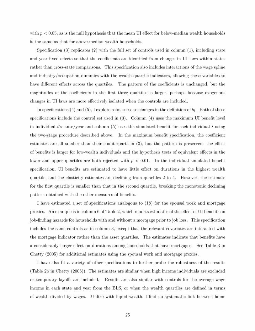
with p < 0:05, as is the null hypothesis that the mean UI e¤ect for below-median wealth households

is the same as that for above-median wealth households.

Speci�cation (3) replicates (2) with the full set of controls used in column (1), including state

and year �xed e¤ects so that the coe¢ cients are identi�ed from changes in UI laws within states

rather than cross-state comparisons. This speci�cation also includes interactions of the wage spline

and industry/occupation dummies with the wealth quartile indicators, allowing these variables to

have di¤erent e¤ects across the quartiles. The pattern of the coe¢ cients is unchanged, but the

magnitudes of the coe¢ cients in the �rst three quartiles is larger, perhaps because exogenous

changes in UI laws are more e¤ectively isolated when the controls are included.

In speci�cations (4) and (5), I explore robustness to changes in the de�nition of bi. Both of these

speci�cations include the control set used in (3). Column (4) uses the maximum UI bene�t level

in individual i�s state/year and column (5) uses the simulated bene�t for each individual i using

the two-stage procedure described above. In the maximum bene�t speci�cation, the coe¢ cient

estimates are all smaller than their counterparts in (3), but the pattern is preserved: the e¤ect

of bene�ts is larger for low-wealth individuals and the hypothesis tests of equivalent e¤ects in the

lower and upper quartiles are both rejected with p < 0:01. In the individual simulated bene�t

speci�cation, UI bene�ts are estimated to have little e¤ect on durations in the highest wealth

quartile, and the elasticity estimates are declining from quartiles 2 to 4. However, the estimate

for the �rst quartile is smaller than that in the second quartile, breaking the monotonic declining

pattern obtained with the other measures of bene�ts.

I have estimated a set of speci�cations analogous to (18) for the spousal work and mortgage

proxies. An example is in column 6 of Table 2, which reports estimates of the e¤ect of UI bene�ts on

job-�nding hazards for households with and without a mortgage prior to job loss. This speci�cation

includes the same controls as in column 3, except that the relevant covariates are interacted with

the mortgage indicator rather than the asset quartiles. The estimates indicate that bene�ts have

a considerably larger e¤ect on durations among households that have mortgages. See Table 3 in

Chetty (2005) for additional estimates using the spousal work and mortgage proxies.

I have also �t a variety of other speci�cations to further probe the robustness of the results

(Table 2b in Chetty (2005)). The estimates are similar when high income individuals are excluded

or temporary layo¤s are included. Results are also similar with controls for the average wage

income in each state and year from the BLS, or when the wealth quartiles are de�ned in terms

of wealth divided by wages. Unlike with liquid wealth, I �nd no systematic link between home

25

equity and the bene�t-duration elasticity. This is consistent with the importance of liquidity, since

accessing home equity is di¢ cult when one is unemployed (Hurst and Sta¤ord 2004). Finally, I �nd

no relationship between the level of bene�ts and durations for a control group of individuals who

do not receive UI . This �placebo test�supports the identi�cation assumption that the variation

in UI bene�ts is orthogonal to unobservable determinants of durations.

In summary, the SIPP data indicate that the link between unemployment bene�ts and dura-

tions documented in earlier studies is driven by a subset of the population that has limited ability

to smooth consumption. This pattern is suggestive of a substantial liquidity e¤ect. As shown in

Figure 1, if one were to assume that substitution e¤ects (@s0@w jB) are similar across unconstrained

and constrained groups, this evidence would be su¢ cient to infer that liquidity e¤ects are large.

However, this assumption may be untenable: constrained households might have di¤erent prefer-

ences (locally or globally) that generate larger substitution e¤ects than unconstrained households.

I therefore turn to a second empirical strategy to identify the magnitude of the liquidity e¤ect.

4 Empirical Analysis II: Severance Pay and Durations

4.1 Estimation Strategy

The ideal way to estimate the liquidity e¤ect would be a randomized experiment where some

job losers are given lump-sum grants or annuity payments while others are not. Lacking such

an experiment, I exploit variation in severance pay policies across �rms in the U.S.26 Severance

payments are made either as lump-sum grants at the time of job loss or in the form of salary

continuation (short-duration annuities).27 All severance packages are unconditional payments that

do not distort marginal incentives to search for a new job. Thus, any causal e¤ect of severance

pay on unemployment durations re�ects a pure liquidity e¤ect.

The most common severance policy is one week of wages per year of service at the �rm. Some

companies have �atter or steeper pro�les with respect to job tenure, and others make no severance

payments at all (Lee Hecht Harrison 2001). Many companies have minimum job tenure thresholds

26Receipt of severance pay intended to supplement UI bene�ts typically does not a¤ect eligibility for UI, althoughsome states can delay bene�ts if the claimant receives �wages in lieu of notice� (Kodryzcki 1998, McCulloch 1998).In Pennsylvania, the unemployment compensation law explicitly states that severance pay does not a¤ect UI bene�ts(Pennsylvania Department of Labor and Industry 2007). Restricting the analysis to the Pennsylvania dataset belowyields results similar to those obtained for the pooled sample.27Since the form of the severance payment cannot be determined in the data, I treat all severance payments as

cash grants. To the extent that the severance is paid as salary continuation, the formula for dWdb

in Corollary 1 willbe more accurate because there is less reliance on the approximate annuity conversion in (13).

26

to be eligible for severance pay, ranging from 3 to 5 years. There is little variation in severance

packages within a given �rm and tenure bracket. Hence, conditional on tenure, the variation in

receipt of severance pay is driven primarily by di¤erences in policies across �rms.

I estimate the e¤ect of severance pay using hazard models similar to those above:

log hi;t = �t + �1sevi + �2sevi � t+ Xi;t (19)

where sevi is an indicator for receipt of severance pay. The coe¢ cient �1 identi�es the e¤ect

of cash grants on job �nding hazards at the beginning of the spell if receipt of severance pay is

orthogonal to other determinants of durations. After estimating the baseline model, I evaluate

this orthogonality condition.

4.2 Data

The data for this portion of the study come from two surveys conducted by Mathematica on behalf

of the Department of Labor. The datasets contain information on unemployment durations, demo-

graphic characteristics, and data on receipt of severance pay. The �rst dataset is a representative

sample of job losers in Pennsylvania in 1991. The second dataset is a sample of unemployment

durations in 25 states in 1998 that oversamples UI exhaustees. I reweight the data using the

sampling weights to obtain estimates for a representative sample of job losers.

For comparability to the preceding results, I make the same exclusions after pooling the two

datasets. I include only prime-age males and discard all individuals who expected a recall at the

time of layo¤ (including temporary layo¤s does not a¤ect the results, as above). These exclusions

leave 2,441 individuals in the sample, of whom 471 (18%) report receiving a severance payment.

Details on the Mathematica datasets and sample construction are given in Appendix C.

Two measures of �unemployment duration�are available in these datasets: (1) an administrative

record of the number of weeks for which UI bene�ts were paid and (2) the number of weeks from

the end date of the individual�s previous job to the (self-reported) start of the next job. For

consistency with the SIPP estimates, I focus on the second measure here. Results are similar, and

more precisely estimated, using the administrative measure.

Table 3 shows summary statistics for severance pay recipients and non-recipients. The sample

generally looks quite similar on observables to the SIPP sample used above. Given the minimum

tenure eligibility requirement, it is not surprising that severance pay recipients have much higher

median job tenures than non-recipients. Correspondingly, severance pay recipients are older and

27

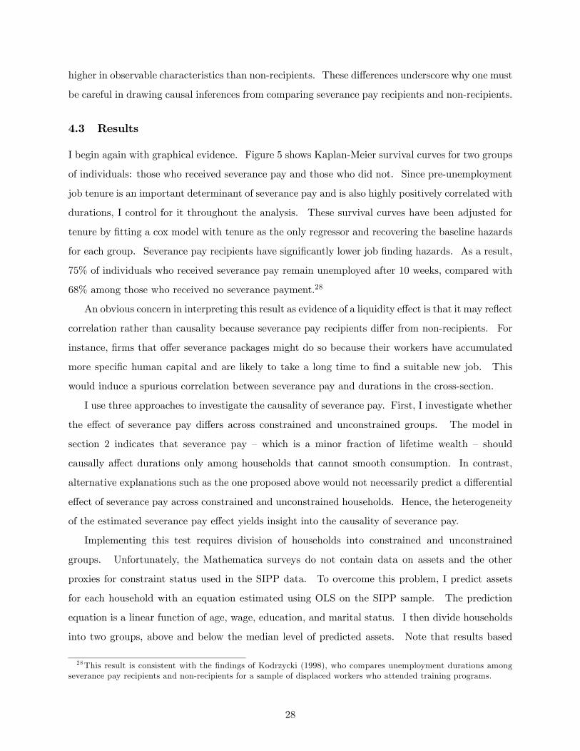
higher in observable characteristics than non-recipients. These di¤erences underscore why one must

be careful in drawing causal inferences from comparing severance pay recipients and non-recipients.

4.3 Results

I begin again with graphical evidence. Figure 5 shows Kaplan-Meier survival curves for two groups

of individuals: those who received severance pay and those who did not. Since pre-unemployment

job tenure is an important determinant of severance pay and is also highly positively correlated with

durations, I control for it throughout the analysis. These survival curves have been adjusted for

tenure by �tting a cox model with tenure as the only regressor and recovering the baseline hazards

for each group. Severance pay recipients have signi�cantly lower job �nding hazards. As a result,

75% of individuals who received severance pay remain unemployed after 10 weeks, compared with

68% among those who received no severance payment.28

An obvious concern in interpreting this result as evidence of a liquidity e¤ect is that it may re�ect

correlation rather than causality because severance pay recipients di¤er from non-recipients. For

instance, �rms that o¤er severance packages might do so because their workers have accumulated

more speci�c human capital and are likely to take a long time to �nd a suitable new job. This

would induce a spurious correlation between severance pay and durations in the cross-section.

I use three approaches to investigate the causality of severance pay. First, I investigate whether

the e¤ect of severance pay di¤ers across constrained and unconstrained groups. The model in

section 2 indicates that severance pay � which is a minor fraction of lifetime wealth � should

causally a¤ect durations only among households that cannot smooth consumption. In contrast,

alternative explanations such as the one proposed above would not necessarily predict a di¤erential

e¤ect of severance pay across constrained and unconstrained households. Hence, the heterogeneity

of the estimated severance pay e¤ect yields insight into the causality of severance pay.

Implementing this test requires division of households into constrained and unconstrained

groups. Unfortunately, the Mathematica surveys do not contain data on assets and the other

proxies for constraint status used in the SIPP data. To overcome this problem, I predict assets

for each household with an equation estimated using OLS on the SIPP sample. The prediction

equation is a linear function of age, wage, education, and marital status. I then divide households

into two groups, above and below the median level of predicted assets. Note that results based

28This result is consistent with the �ndings of Kodrzycki (1998), who compares unemployment durations amongseverance pay recipients and non-recipients for a sample of displaced workers who attended training programs.

28

on predicted assets (using the same prediction equation) and reported assets are similar in the

SIPP data: the total elasticity of duration w.r.t. UI bene�ts is much larger among households with

predicted assets below the median than for those above the median. Hence, the predicted asset

measure succeeds in identifying the households whose search behavior is sensitive to UI bene�ts.

Figures 6a-b replicate Figure 5 for the two groups. Figure 6a shows that receipt of severance pay

is associated with a large increase in survival probabilities for constrained (low asset) households.

Figure 6b shows that severance pay has a much smaller e¤ect on search behavior for households

that are likely to be wealthier. Results are similar if households are split into constrained and

unconstrained groups on the basis of age or income alone. Results are also una¤ected by changes

in the functional form of the asset prediction equation, prediction via quantile regression instead of

OLS, or trimming of outliers. The fact that severance pay a¤ects durations only in the group of

households that are sensitive to UI bene�ts (those who are likely to be constrained) supports the

claim that liquidity e¤ects drive a substantial portion of the UI-duration link.

As a second approach to examining the causality of severance pay, I assess the sensitivity of

the severance pay e¤ect to controlling for observed heterogeneity. I estimate variants of the Cox

model in (19), censoring all durations at 50 weeks as in the SIPP data. I �rst estimate a model

with only a linear tenure control and a the time-varying interaction of severance pay with weeks

unemployed. I then estimate the model with the following control set: ten piece linear splines

for log pre-unemployment wage and job tenure; dummies for prior industry, occupation, and year;

and controls for age, marital status, and education (using a dummy for dropout status and college

graduation). The �rst two columns of Table 4 show that receipt of severance pay is estimated to

lower the job-�nding hazard at the beginning of the spell by �1 = �18% in the tenure-control and

�1 = �23% in the full-control speci�cation. The estimated value of �2 = 1:3% (s.e. = 0:2%) in

both speci�cations. The e¤ect of severance pay on search intensity diminishes over time, as one

might expect if individuals deplete the grant over the course of the spell.

Speci�cations (3) and (4) estimate separate severance pay coe¢ cients for constrained (below-

median predicted assets) and unconstrained (above-median) households. The baseline hazards

are strati�ed by predicted wealth group (above/below median) and the wage spline and indus-

try/occupation dummies are interacted with the predicted wealth dummy, as in the SIPP speci�-

cations.29 Consistent with Figure 6, the estimates indicate that severance pay reduces initial job

29Unlike in the SIPP speci�cations, I restrict the time interaction of severance pay with weeks unemployed to be thesame across wealth groups here in order to increase power. Introducing an interaction yields similar point estimatesbut larger standard errors because the number of severance pay recipients is relatively small.

29

�nding hazards in the low-wealth group by 46-49%, but has little or no e¤ect in the high-wealth

group. The hypothesis that the e¤ect of severance pay is the same in the low and high wealth

groups is rejected with p < 0:01. Predicting whether the individual is above or below median

wealth directly in the �rst stage, and interacting the predicted probability with the severance pay

dummy when estimating the Cox model yields the same conclusion.

Finally, as a third robustness check, I test whether larger severance payments lead to longer

unemployment durations. I implement this intensive margin test by investigating whether the

e¤ect of severance pay receipt di¤ers by individuals� job tenure. Since the severance amount

is an increasing function of job tenure, the indicator for receipt of severance pay should have a

larger e¤ect on durations among individuals with long job tenure.30 I divide the pooled sample

(including both severance recipients and non-recipients) into two groups �short and long tenure

�based on whether their job tenure is above or below the median for severance recipients (4.83

years). Based on data in Lee Hecht Harrisson (2001), the mean severance amount conditional on

receipt of severance is equivalent to 2 weeks of wages in the short tenure group vs. 13 weeks of

wages in the long tenure group (see Appendix C).

Columns 5 and 6 of Table 4 replicate speci�cations 3 and 4, stratifying the baseline hazards by

the short job tenure indicator and interacting it with the severance pay indicator. For individuals

who have short job tenure, receipt of severance pay reduces initial job �nding hazards by 10-14%,

compared with 25-34% for the long tenure group.31 The hypothesis that the e¤ect of severance

pay is the same in the low and high tenure groups is rejected with p < 0:03.

Although these �ndings all point toward a substantial liquidity e¤ect, the evidence cannot be

viewed as fully conclusive because the variation in cash grants is not randomized. One might,

for instance, be concerned that low wealth workers with job-speci�c capital are especially likely

to select into and stay at �rms that o¤er severance payments, explaining the patterns in Table 4.

Reassuringly, in a followup study that exploits quasi-experimental variation in severance payments

created by a discontinuity in the Austrian severance pay system, Card, Chetty, and Weber (2007)

document a substantial e¤ect of severance pay on durations, consistent with the evidence here.

Further research along these lines is needed to obtain more precise and compelling estimates of the

30Data on actual severance amounts are available for a subset of the Pennsylvania dataset. I �nd a positiveassociation between the reported amounts and durations, but the results are not statistically signi�cant because ofthe small number of observations.31An alternative interpretation of speci�cations 5 and 6 is that tenure is used as an instrument for the severance

amount, with the direct e¤ects of tenure on duration netted out by comparison to the group of non-recipients. Thecorrelation between job tenure and durations is larger among severance pay recipients than non-recipients, which isconsistent with a liquidity e¤ect because the severance amount rises with job tenure for severance recipients.

30

liquidity e¤ect in the U.S.

5 Calibration: Welfare Implications

I now use the hazard model estimates to calculate the average liquidity to moral hazard ratio in

the population and the average welfare gain from raising b. Let h0 denote the job �nding hazard

in the �rst week for an agent who receives the mean UI bene�t b and does not receive a severance

payment. Let hs1 denote the hazard for an individual who receives the severance payment and hb1

denote the hazard for an individual whose UI bene�t level is doubled. Using the approximation in

(13), we obtain@s0@ajB=

@s0@b

= B@s0@A

=@s0@b

=Bb

S

[hs1 � h0]=h0[hb1 � h0]=h0

where b denotes the mean weekly UI bene�t and S denotes the mean total value of the severance

payment. Based on a survey of �rms by Lee Hecht Harrison (2001), the mean severance payment

equals 10.7 weeks of wages (see Appendix C). At the mean bene�t level of b = 0:5w, this implies

S = 21:4b �that is, receipt of severance pay is equivalent to an annuity payment of b per week for

21.4 weeks. The full-controls estimates from column 1 of Table 2 and column 2 of Table 4 imply

hb1=h0 = exp(�0:58) and hs1=h0 = exp(�0:23). It follows that

@s0@ajB=

@s0@b

=exp(�0:23)� 1exp(�0:53)� 1 �

26

21:4= 0:6.

Around the level of bene�ts observed in the data (b � 0:5w), the liquidity e¤ect accounts for roughly

60% of the e¤ect of marginal changes in the bene�t level on unemployment durations.

Welfare Gain of UI. To calculate "D;b, recall from speci�cation 1 of Table 2 that the e¤ect of

bene�ts on the hazard rate does not vary signi�cantly over the spell. Using the approximation that

the bene�t elasticity and baseline hazard rates are constant, D = 1h and "D;b = �

@ log h0@ log b = 0:53.

32

Shimer and Werning (2007) report that there are 7.7 million unemployed individuals and 135 million

32The elasticity "D;b called for in (14) includes the e¤ect of the change in � . The estimated elasticity does not fullyinclude the e¤ect of � because the variation UI bene�ts a¤ects only some agents whereas taxes are levied more broadly.This discrepancy is likely to be quantitatively unimportant because the UI tax rate is very small (� < 0:01w). Inthe numerical simulations, the elasticities with � �xed and � variable are virtually identical.

31

workers in the U.S.: � = 135142:7 = 0:946. Using the approximation that "D;b = "DB ;b, (14) yields

dW

db(b = 0:5w) =

1� ��

DBDf@s0@ajB=(

@s0@ajB �

@s0@b)� "DB ;b

�g

=1� 0:9460:946

� 15:824:3

� (0:60:4

� 0:53

0:946) = 0:04

Starting from b = 0:5w, a $1 balanced-budget increase in the weekly bene�t level would have raised

each individual�s utility by the equivalent of a 4 cent increase in the weekly wage, or about $2.00

per year. Aggregating over the population, the welfare gain of raising the UI bene�t level by a

dollar is equivalent to an increase in GDP of $290 million. Starting from a mean bene�t of $200

per week, raising the bene�t level by 10% would yield an aggregate welfare gain equivalent to about

$5.9 billion, roughly 0.05 percent of GDP.

It is important to recognize that these welfare gain calculations are valid only locally around

b = 0:5w. The liquidity e¤ect and marginal welfare gain of UI will be larger when b is low

and small when b is high, as illustrated in the numerical simulations in section 2. The local

welfare gain estimate does tell us that the optimal wage replacement rate for UI exceeds 50% since

dWdb (b = 0:5w) > 0. In addition, the evidence suggests that a replacement rate near 50% may be

near optimal since dWdb (b = 0:5w) is small.

33

It is interesting to compare the welfare implications of the revealed preference approach with

those of previous studies. Hansen and Imrohoglu (1992) �nd that the optimal replacement rate is

65% if moral hazard is low but less than 10% if moral hazard is high in their baseline simulation.

They conclude that evidence on moral hazard is needed to assess which case is relevant. The

present paper provides empirical evidence that the low moral hazard case is the relevant one, and

yields welfare implications consistent with Hansen and Imrohoglu�s simulation for that case. Baily

(1978) and Gruber (1997) use a consumption-based exact identi�cation approach to show that

@W@b (b = 0:5w) < 0 using estimates of the consumption drop during unemployment. Indeed, their

preferred calibrations using log utility imply an optimal bene�t rate close to zero. The reason for

the sharp discrepancy is that the liquidity e¤ect estimated here is inconsistent with the relatively low

degrees of risk aversion considered by Baily and Gruber.34 Shimer and Werning (2007) implement

33This calculation ignores �rm layo¤ behavior (Feldstein 1978, Topel 1983) and general equilibrium e¤ects (Ace-moglu and Shimer 1999). Generalizing the formula to account for these factors would be very valuable.34Recall that @s0

@ajB= @s0@b = 0:6 =

u0(cu)�u0(ce)u0(cu) ' ce�cu

cuwhere denotes the coe¢ cient of relative risk aversion at

cu. Gruber estimates cuce= 0:9, which requires ' 5 to be consistent with a 60% liquidity e¤ect. A strength of the

formula proposed here is that it does not require estimate of risk aversion, which could plausibly be as high as = 5in the context of moderate shocks such as unemployment but much lower in other contexts (Chetty and Szeidl 2007).

32

their reservation-wage formula using an estimate of the sensitivity of reservation wages to bene�ts

from Feldstein and Poterba (1984). They �nd that a $1 increase in the bene�t level would yield a

net welfare gain equivalent to raising GDP by $2.4 billion, four times larger than the estimate here.

As Shimer and Werning observe, the credibility of existing reservation wage elasticity estimates is

questionable, particularly in view of more recent evidence that UI bene�t levels have little impact

on subsequent wage rates (e.g. Card, Chetty, Weber 2007, van Ours and Vodopivec 2008).

Alternative Policy Instruments: Loans. In the analysis above, the unemployment bene�t is

used to facilitate both intertemporal smoothing and smoothing across states. A natural alternative

instrument to resolve credit market failures is the provision of loans or UI savings accounts ((Feld-

stein and Altman (1998), Shimer and Werning (2006)). Although a formal analysis of optimal

policy with multiple instruments is outside the scope of this paper, the numerical simulations can

be used to gain some insight into how much of the welfare gain of UI could be obtained using loans.

Suppose the government provides a loan of $G upon job loss that must be repaid within GT

weeks. With this loan, the agent�s budget constraint is At � �(L +G) for t � GT and At � �L

for t > GT . Let us compare the welfare gain from increasing the government loan by $B (dWdG =

B dJ0dG =

dJ0dw ) with the welfare gain from raising the UI bene�t by $1 for B periods (dWdb =

dJ0dG =

dJ0dw ).

Assume b = 0:5w and all other parameters as in Figure 2. The solid curves in Figure 7 plot dWdG

and dWdb as a function of G when the government loan has to be repaid by death (GT = T = 500).

The dashed curves plot dWdG (G) anddWdb (G) for a short-term loan (GT = 104).

The simulations have three lessons. First, the welfare gains from providing long-term liquidity

can be quite large. The welfare gain of initiating a long-term government loan when b = 0:5w

is dWdG (G = 0) = 0:044. The marginal welfare gain of increasing b falls rapidly with G: when

G = 5000, dWdb is 40% of the value ofdWdb when G = 0. Substantial welfare gains can be achieved by

correcting credit market failures while leaving insurance markets incomplete because unemployment

shocks are small relative to permanent income.

Second, short-term loans are much less valuable than long-term loans. The marginal welfare

gain of a loan that lasts for less than 11 months is zero in this numerical example because the

private market borrowing limit (L = �1000) begins to bind only at t = 47. The welfare gain from

the two year loan plotted in the �gure is close to the value of the permanent loan initially, but

declines rapidly as G rises. Once the loan amount exceeds $3,600, the marginal value of the loan

becomes 0 because the borrowing constraint becomes slack for t � 104. The UI bene�t, in contrast,

retains a marginal value of dWdb = 0:018 because consumption �uctuates signi�cantly across states

33

even when G > $3; 600. Intuitively, a job loser is reluctant to take up a lot of short-term debt even

though it would help him smooth consumption because of the risk of a long spell of unemployment

(an example of precautionary savings behavior).

The �nal lesson pertains to the welfare value of using loans instead of the existing UI system.

The long term loan generates a strictly larger welfare gain than the UI bene�t because UI has an

e¢ ciency cost, whereas loan provision is non-distortionary in this model. However, the di¤erence

in the welfare gain from a $1 increase in b and a comparable increase in even the �rst-best costless

loan is less than a 0.5 cents of weekly wages on average. The di¤erence is small because the moral

hazard distortion caused by UI is small in practice. It is therefore critical to quantify the moral

hazard cost of loans to determine whether loans or subsidies for job search are a better policy to

facilitate consumption smoothing.

Other Policy Implications. Recent evidence that UI does not smooth consumption for house-

holds with high assets (e.g. Browning and Crossley 2001) has been interpreted as a point in favor of

means-testing temporary income support programs. But UI does not a¤ect unemployment dura-

tions signi�cantly for this group either. Since means-testing generates a distortionary incentive to

save less, a universal bene�t may maximize welfare. In addition, the evidence above implies that

e¤orts to shorten unemployment durations through job-�nding bonuses or more stringent search re-

quirements would yield welfare gains 60% smaller than suggested by prior studies which attributed

the entire duration response to a substitution e¤ect.

6 Conclusion

This paper has proposed and implemented an �exact identi�cation�approach to welfare analysis.

In particular, we showed that the welfare gain from increasing the unemployment bene�t level can

be well approximated by estimating a pair of high-level elasticities rather than identifying the full

set of primitives. The central intuition is that UI bene�ts a¤ect search behavior through two

channels: a welfare-enhancing �liquidity e¤ect�and a welfare-reducing moral hazard e¤ect. The

ratio of the liquidity e¤ect to the moral hazard e¤ect is a su¢ cient statistic for the welfare gain

of raising the bene�t level in a general environment. Using data from the U.S., I estimate that

the liquidity e¤ect accounts for 60% of the marginal e¤ect of UI bene�ts on durations at current

bene�t rates. This estimate implies that a bene�t equal to 50% of the pre-unemployment wage is

near optimal in a UI system that pays constant bene�ts for six months.

Although this paper has focused on unemployment, the theoretical concepts have broader ap-

34

plicability. Revealed preference can be used to calculate the welfare gains from social and private

insurance policies by separating moral hazard and liquidity e¤ects. For example, one can calculate

the value of a health insurance program by estimating the extent to which an agent�s medical ex-

penditures would di¤er if he were paid a lump-sum bene�t rather than an indemnity bene�t that

covers health expenses. This method does not require data on the outcomes of insurance provision,

such as health, consumption, or job match quality, which have proved to be di¢ cult to measure.35

More generally, developing exact identi�cation strategies to analyze optimal policy in contexts

beyond insurance should be a high priority for further work. Such strategies o¤er the promise

of combining the best feature of reduced-form empirical analysis �transparent and credible iden-

ti�cation �with the bene�t of structural models � the ability to make precise statements about

welfare.

35See Nyman (2003) and Autor and Duggan (2007) for evidence on moral hazard vs. liquidity e¤ects in health anddisability insurance.

35

ReferencesAcemoglu, Daron and Robert Shimer. 1999. �E¢ cient Unemployment Insurance.�Journal of

Political Economy 107 (October): 893-928.Acemoglu, Daron and Robert Shimer. 2000. �Productivity Gains from Unemployment Insur-

ance.�European Economic Review 44 (June): 1195-1224.Anderson, Patricia and Bruce Meyer. 1997. �Unemployment Insurance Takeup Rates and the

After-Tax Value of Bene�ts.�Quarterly Journal of Economics 112 (August): 913-937.Autor, David and Mark Duggan. 2007. �Income vs. Substitution E¤ects in Disability Insur-

ance.�American Economic Review Papers and Proceedings 97 (May): 119-124.Baily, Martin N. 1978. �Some Aspects of Optimal Unemployment Insurance.�Journal of Public

Economics 10 (December): 379-402.Bloemen, Hans and Elena Stancanelli. 2005. �Financial Wealth, Consumption Smoothing and

Income Shocks Arising from Job Loss.�Economica 72 (August): 431-452.Blundell, Richard, Luigi Pistaferri, and Ian Preston. 2008. �Consumption Inequality and

Partial Insurance.�American Economic Review forthcoming.Browning, Martin and Thomas Crossley. 2001. �Unemployment Insurance Levels and Con-

sumption Changes.�Journal of Public Economics 80 (April): 1-23.Card, David, Raj Chetty, and Andrea Weber. 2007. �Cash-on-Hand and Competing Models of

Intertemporal Behavior: New Evidence from the Labor Market.� Quarterly Journal of Economics122(4): 1511-1560.

Carroll, Christopher. 1997. �Bu¤er-Stock Saving and the Life Cycle/Permanent Income Hy-pothesis,�Quarterly Journal of Economics CXII: 1-56.

Chetty, Raj. 2003. �Consumption Commitments, Unemployment Durations, and Local RiskAversion,�Working Paper No. 10211 (December) NBER, Cambridge, MA.

Chetty, Raj. 2005. �Why do Unemployment Bene�ts Extend Unemployment Durations? MoralHazard vs. Liquidity.�Working Paper No. 11760 (November) NBER, Cambridge, MA.

Chetty, Raj. 2006a. �A General Formula for the Optimal Level of Social Insurance.�Journalof Public Economics 90 (November ): 1879-1901.

Chetty, Raj. 2006b. �A New Method of Estimating Risk Aversion.�American Economic Review96 (December): 1821-1834.

Chetty, Raj and Adam Szeidl. 2007. �Consumption Commitments and Risk Preferences.�Quarterly Journal of Economics 122 (May): 831-877.

Chetty, Raj and Emmanuel Saez. 2008. �Optimal Taxation and Social Insurance with PrivateInsurance Markets�UC-Berkeley mimeo.

Cochrane, John. 1991. �A Simple Test of Consumption Insurance.�Journal of Political Econ-omy 99 (January): 957-76.

Cullen, Julie and Jonathan Gruber. 2000. �Does Unemployment Insurance Crowd Out SpousalLabor Supply?�Journal of Labor Economics 18 (July): 546-572.

Employment and Training Administration, Signi�cant Provisions of State Unemployment In-surance Laws. various years. Washington D.C.: U.S. Government Printing O¢ ce .

Feldstein, Martin. 1978. �The E¤ect of Unemployment Insurance on Temporary Layo¤s.�American Economic Review 68 (December): 834-46.

Feldstein, Martin and Daniel Altman. 1998. �Unemployment Insurance Savings Accounts.�Working Paper No. 6860 (December) NBER, Cambridge, MA.

Feldstein, Martin and James Poterba. 1984. �Unemployment Insurance and ReservationWages.�Journal of Public Economics 23 (February-March ): 141-67.

Gruber, Jonathan. 1997. �The Consumption Smoothing Bene�ts of Unemployment Insurance.�American Economic Review 87 (March): 192-205.

36

Gruber, Jonathan. 1998. �Unemployment Insurance, Consumption Smoothing, and PrivateInsurance: Evidence from the PSID and CEX.�Research in Employment Policy 1: 3-31.

Gruber, Jonathan. 2007. Public Finance and Public Policy. New York: Worth Publishers.Hansen, Gary and A. Imrohoroglu. 1992. �The Role of Unemployment Insurance in an Economy

with Liquidity Constraints and Moral Hazard.�Journal of Political Economy 100: 118-142.Hurst, Erik and Frank Sta¤ord. 2004. �Home Is Where the Equity Is: Mortgage Re�nancing

and Household Consumption.�Journal of Money, Credit, and Banking 36 (December): 985-1014.Johnson, David, Jonathan A. Parker and Nicholas S. Souleles. 2006. �Household Expenditure

and the Income Tax Rebates of 2001.�American Economic Review 96 (December ): 1589-1610.Kodrzycki, Yolanda. 1998. �The E¤ects of Employer-Provided Severance Bene�ts on Reem-

ployment Outcomes.�New England Economic Review (November): 41-68.Krueger, Alan and Bruce Meyer. 2002. �Labor Supply E¤ects of Social Insurance.� in A.

Auerbach and M. Feldstein, eds. Handbook of Public Economics Vol 4. North-Holland: Amsterdam.Hopenhayn, Hugo and Juan Pablo Nicolini. 1997. �Optimal Unemployment Insurance,�Journal

of Political Economy 105 (April): 412�438.Lee Hecht Harrison. 2001. �Severance and Separation Bene�ts: Bridges for Employees in

Transition.�monograph, Woodcli¤ Lake, NJ: Lee Hecht Harrison.Lentz, Rasmus. 2008. �Optimal Unemployment Insurance in an Estimated Job Search Model

with Savings.�Review of Economic Dynamics forthcoming.Lentz, Rasmus and and Torben Tranaes. 2005. �Job Search and Savings: Wealth E¤ects and

Duration Dependence.�Journal of Labor Economics 23 (July): 467-489.Lucas, Robert E., Jr.. 1987. Models of Business Cycles. Basil Blackwell, New York.McCall, John J. 1970. �Economics of Information and Job Search.� Quarterly Journal of

Economics 84 (February): 113-126.McCulloch, Kenneth. 1998. Termination of Employment: Employer and Employee Rights.

Boston: Warren, Gorham and Lamont.Meyer, Bruce. 1990. �Unemployment Insurance and Unemployment Spells.�Econometrica 58

(July): 757-782.Mo¢ tt, Robert. 1985. �Unemployment insurance and the distribution of unemployment spells.�

Journal of Econometrics 28 (April): 85�101.Nyman, John. 2003. The Theory of Demand for Health Insurance. Stanford: Stanford

University Press.Pennsylvania Department of Labor and Industry. 2007. �Unemployment Compensation Regu-

lations.�Available at http://www.dli.state.pa.us/landi/cwp/view.asp?a=185&q=170005.Shimer, Robert and Ivan Werning. 2006. �Liquidity and Insurance for the Unemployed.�FRB

Minneapolis Sta¤ Report #366 (December).Shimer, Robert and Ivan Werning. 2007. �Reservation Wages and Unemployment Insurance.�

Quarterly Journal of Economics 122(3): 1145-1185.Sullivan, James. 2007. �Borrowing During Unemployment: Unsecured Debt as a Safety Net.�

Journal of Human Resources forthcoming.Topel, Robert. 1983. �On Layo¤s and Unemployment Insurance.�American Economic Review

73 (September): 541-549.van Ours, Jan and Milan Vodopivec. 2008. �Does Reducing Unemployment Insurance Gen-

erosity Reduce Job Match Quality?�Journal of Public Economics forthcoming .Wolpin, Kenneth I. 1987. �Estimating a Structural Search Model: The Transition from School

to Work.�Econometrica 55(4): 801-817.Zeldes, Stephen P. 1989. �Consumption and Liquidity Constraints: An Empirical Investiga-

tion.�Journal of Political Economy 97(April): 305-346.

37

Appendix A: Proofs

Derivation of decomposition in (9).

For any variable x 2 fa; b; wg and s � T , let @y@x js =sPt=0

@y@xt

denote the e¤ect of increasing x in

all periods 0 to s on y. Then it follows that

@s0@xjs =

1

00(s0)[@V0@xjs �

@U0@x

js] (20)

Note that @s0@b jB =@s0@b because UI bene�ts and the annuity last for only B periods by assumption.

Exploiting the envelope conditions from agent optimization, we obtain the following derivatives forthe value functions:

@U0@b

= u0(cu0) +B�1Pt=1

tQi=1(1� si)u0(cut )

@V0@b

= 0

@U0@w

jB = s1(B � 1)v0(ce1) +B�1Pt=2[tQi=2(1� si�1)]st(B � t)v0(cet )

@V0@w

jB = Bv0(ce0)

@U0@a

jB =@U0@b

+@U0@w

jB@V0@ajB =

@V0@w

jB

Using these expressions and equation (20), it follows that

@s0@b

=@s0@ajB �

@s0@w

jB.

Proof of Proposition 1. To begin, observe that the unconditional average marginal utility ofconsumption while employed over the �rst B periods is

E0;B�1v0(cet ) =1

B �DB[s0Bv

0(ce0) +B�1Pt=1[tQi=1(1� si�1)]st(B � t)v0(cet )]

=1

B �DB[(1� s0)

@U0@w

jB + s0@V0@w

jB]

The average marginal utility of consumption while employed conditional on �nding a job in period0 is

E0;B�1v0(ce0) = v0(ce0) =1

B

@V0@w

jB

To derive (14), recall that J0 = (1� s0)U0(b; �) + sV0(b; �) + (s0). Therefore

dJ0db

= (1� s0)f@U0@b

� @U0@w

d�

dbg � s0

@V0@w

d�

db(21)

= �(1� s0) 00@s0@b

� d�

db(T �D)E0;T�1v0(cet )

Next, I normalize the expression for dJ0db by the expected welfare gain from increasing the wage by

38

$1, dJ0dw = (T �D)E0;T�1v0(cet ):

@W

@b=dJ0db

=dJ0dw

= � 1

T �D(1� s0)

E0;T�1v0(cet ) 00@s0@b

� d�

db

Using (20) and the de�nitions of E0;B�1v0(ce0) and E0;B�1v0(cet ), we obtain

@s0@w

jB =1

001

1� s0fBv0(ce0)� (B �DB)E0;B�1v0(cet )g

This expression implies that

@s0@w

jB=@s0@w

=DBE0;B�1v0(cet ) +B(v

0(ce0)� E0;B�1v0(cet ))DE0;T�1v0(cet ) + T (v0(c

e0)� E0;T�1v0(cet ))

Combining the preceding equations, some algebra yields

dW

db=

DBT �Df�

E0;B�1v0(cet )� v0(ce0)E0;T�1v0(cet ))

B

DB� E0;B�1v0(cet )E0;T�1v0(cet ))

g(@s0@a

@s0@w jB

� 1)� d�

db

Di¤erentiating the government�s budget constraint, we obtain

d�

db=

DBT �D (1 + "DB ;b + "D;b

D

(T �D))

Plugging this expression into the formula for dWdb above and collecting terms yields (14). QED.

Extension 1: Ex-ante Behavior. The main steps of the proof are the same as in Proposition1. I �rst write dWdb in terms of marginal utilities as in (10), and then show how this representationcan be linked to (@s0@a jB)jA0;z and

@s0@b jA0;z �e¤ects of a and b on s0 holding A0 and z �xed. Recall

that dWdb �dJ�1db =

T�1Pt=�1

dJ�1dwt

. Computing these derivatives explicitly gives:

dJ�1db

= �v0(ce�1)d�

db� (1� p)Tv0(A0 � !(z) +

Pwt

T� �)d�

db+ p

dJ0db

= �v0(ce�1)d�

db� (1� p)Tv0(A0 � !(z) +

Pwt

T� �)d�

db+ pf(1� s0)f

@U0@b

� @U0@w

d�

dbg � s0

@V0@w

d�

dbg

T�1Xt=�1

dJ�1dwt

= (T + 1� pD)E0;T�1v0(cet )

Using the approximation that v0(cet ) = v0(ce0) for all t, these expressions simplify to:

dJ�1db

= p(1� s0)@U0@b

� d�

db(T + 1� pD)v0(ce0)

T�1Xt=�1

dJ�1dwt

= (T + 1� pD)v0(ce0)

=) dW

db=

p(1� s0)(T + 1� pD)

@U0@b

=v0(ce0)�d�

db

This marginal-utility representation is analogous to equation (21) in the proof of Proposition 1.

39

To rewrite this equation in terms of moral hazard and liquidity e¤ects, consider the followingcomparative statics:

@s0@bjA0;z = � 1

00@U0@b

(@s0@ajB)jA0;z =

1

00[@V0@ajB �

@U0@a

jB] = �1

00@U0@b

+1

001

1� s0DBv

0(cet )

Combining these equations, it is easy to see that:

1 +�@s0@a jA0;z

@s0@a jA0;z �

@s0@b jA0;z

= (1� s0)@U0@b

=v0(cet )

Di¤erentiating the government�s budget constraint and using the approximation "D;b = "DB ;b, weobtain

d�

db=

pDBT + 1� pD (1 +

T + 1

T + 1� pD"DB ;b)

Finally, plugging these expressions into the formula for dWdb above and collecting terms yields

dW

db=1� ��

DBDfR� "DB ;b

�g

where � = T+1�pDT+1 and R =

�( @s0@ajB)jA0;z

(@s0@ajB)jA0;z�

@s0@bjA0;z

is the liquidity to moral hazard ratio, holding

�xed ex-ante behaviors.

Extension 2: Stochastic Wage O¤ers

Suppose that with probability st (controlled by search intensity) the agent is o¤ered a wagew � wm + F (w). Assume no recall of previous o¤ers and i.i.d. draws across periods. The agentfollows a reservation-wage policy: in each period t, there is a threshold Rt such that the agentaccepts a job only if the wage w > Rt (McCall 1970). I generalize Corollary 1 to this model in thefollowing steps: (1) specify the value functions, (2) write the marginal welfare gain from raising b interms of expected marginal utilities, and (3) relate the gap in marginal utilities to the comparativestatics of search intensity. For simplicity, assume B = T .

The value function for an individual with assets At who �nds and accepts a job at the beginningof period t that pays a wage w is

Vt(w;At) = maxAt+1�L

v(At �At+1 + w) + Vt+1(w;At+1).

The value function for an individual who fails to �nd a job at the beginning of period t and remainsunemployed is

Ut(At) = maxAt+1�L

u(At �At+1 + bt) + Jt+1(At+1)

where Jt+1(At+1) is the value of entering period t+ 1 unemployed with assets A. The probabilityof �nding and accepting a job in period t is stP (w > Rt) where P (w > Rt) =

R1RtdF (w). It follows

thatJt(At) = max

st;RtstP (w > Rt)EVt + (1� stP (w > Rt))Ut(At)� (st)

40

where

EVt = E[Vt(w;At)jw > Rt] =1

P (w > Rt)

Z 1

Rt

[Vt(w;At)dw

represents the expected value of being employed conditional on receiving an acceptable o¤er. LetP = P (w > R0) in what follows. The marginal welfare gain from raising the UI bene�t is:

dJ0db

= (1� Ps0)@U0@b

� d�

dbf(1� Ps0)

@U0@wm

+ Ps0@EV0@wm

g.

The marginal welfare gain of raising the wage by $1 in all states and periods is

dJ0dwm

= (1� Ps0)@U0@wm

+ Ps0@EV0@wm

= (T �D)Ev0(cet ) (22)

where Ev0(cet ) denotes the average marginal utility of consumption while employed. The latterequality follows from di¤erentiating the value functions and exploiting the envelope conditions forst and Rt, as in the derivation of (9) above.

Combining these equations, the money-metric measure for the welfare gain from raising b is

dW

db=dJ0db

=dJ0dwm

= (1� Ps0)@U0@b

=(T �D)Ev0(cet )�d�

db

To write this expression in terms of the liquidity and moral hazard e¤ects on search intensity, notethat the �rst order condition for s0 is:

PEV0(A0; a)� PU0(A0; a; b) = 0(s0)

which is a simple generalization of (4), replacing the value function V with its expected valueand integrating over the wage distribution. Di¤erentiating the �rst-order condition yields thefollowing comparative statics: @s0=@b = �P @U0

@b = 00(s0), @s0=@a = Pf@EV0@a � @U0

@a g= 00(s0), and

@s0=@wm = Pf@EV0@wm� @U0

@wmg= 00(s0).

If the agent �nds a job in period 0, the average marginal utility of consumption (integrating over

the wage distribution) is @EV0@wm= TEv0(ce0). Using (22), it follows that

@U0@wm

=(T�D)Ev0(cet )�Ps0Tv0(ce0)

1�Ps0 .Hence the e¤ect of raising the wage in all states and periods by $1 on search intensity is

@s0@wm

= PfTEv0(ce0)�(T �D)Ev0(cet )� Ps0Tv0(ce0)

1� Ps0g= 00(s0)

To simplify this expression, make the approximation that the average marginal utility of consump-tion is constant over time, i.e. Ev0(ce0) = Ev0(cet ). This approximation implies

@s0@wm

=P

00DEv0(cet )

1� Ps0

Using the expressions for @s0@b and@s0@wm

, we obtain

dW

db= � (1� Ps0)( 00(s0)@s0=@b)=P

(1� Ps0)( 00(s0)@s0=@wm)=PD

T �D � d�

db

41

Di¤erentiating the government�s budget constraint yields

d�

db=

D

T �D (1 + "D;bT

(T �D))

Plugging in this expression and collecting terms, we obtain

dW

db=1� ��

f� @s0=@a

@s0=@a� @s0=@b� "DB ;b

�g (23)

which is precisely the same formula as in Corollary 1.The problem in implementing (23) empirically is that the re-employment hazard in period t

is ht = st[1 � F (Rt)]. Therefore changes in ht that are observed in the data cannot be directlymapped to changes in st. To address this problem, note that the expected accepted wage is

wt = E[wtjwt > Rt] =

Z 1

Rt

wtdF (wt)=[1� F (Rt)]

Letting the density of the wage distribution be denoted by f(w), we have

@wt@Rt

= (wt �Rt)f(Rt)

(1� F (Rt))(24)

For any variable x 2 fa; bg, the e¤ect of a change in x on the average accepted wage is

@wt@x

= (wt �Rt)f(Rt)

1� F (Rt)@Rt@x

The e¤ect of a change in x on the re-employment hazard in period t is

@ log ht@x

=@ log st@x

� f(Rt)

[1� F (Rt)]@Rt@x

(25)

Combining these equations yields

@ log st@x

=@wt@x

1

wt �Rt+@ log ht@x

Finally, plugging this expression with x = a and x = b into (23) gives

dW

db=1� ��

f�@w0@a

1w0�R0 +

@ log h0@a

[@w0@a1

w0�R0 +@ log h0@a ]� [@w0@b

1w0�R0 +

@ log h0@b ]

� "DB ;b�

g (26)

This formula shows that one can calculate dWdb when wage o¤ers are stochastic using information

about the reservation wage R0 and the e¤ect of bene�ts and cash grants on mean accepted wages.If @xt@A0

= 0 and @xt@b = 0, (26) collapses back to

dW

db=1� ��

f� @h0=@a

@h0=@a� @h0=@b� "DB ;b

�g,

which is exactly the formula implemented in section 5.

Extension 3: Heterogeneity. For simplicity, consider the baseline model with T = 1. Supposethe economy has N individuals, indexed by i. Let ui, vi, i, denote the consumption utility

42

functions of agent i. Let Ai0 denote initial assets and wi0 denote the wage. The government�s

objective is to maximize the sum of the agent�s expected utilities subject to the constraint thattotal bene�ts paid equal totals taxes collected in expectation:

maxb0

fW (b0) = NPi=1f(1� si0(b0))ui(Ai0 + b0) + si0(b0)vi(Ai0 + wi0 � �)� i(si0(b0))g

s.t. b0NPi=1(1� si0(b0)) = �

NPi=1

si0(b0)

Let Es0 =NPi=1

si0=N denote mean search intensity in the population, Eu0(cu0) =NPi=1(1�si0)u0i(cu0;i)=

NPi=1(1�

si0) denote mean marginal utility for those who are unemployed, and Ev0(ce0) =NPi=1

si0v0i(c

e0;i)=

NPi=1

si0

denote mean marginal utility for those who are employed. It is straightforward to establish that:

dfWdb0

=NPi=1(1� si0)u0i(cu0;i)�

NPi=1

si0v0i(c

e0;i)

d�

db0

= N(1� Es0)Eu0(cu0)�NEs0Ev0(ce0)d�

db0

The marginal welfare gain of raising the wage rate by $1 for all agents isNPi=1

si0v0i(c

e0;i) = Es0Ev0(ce0).

Noting that d�db0= 1�Es0

Es0 � 1(Es0)2 b0

dEs0db0, it follows that

dW

db0=dfWdb0

=Es0Ev0(ce0) = N1� Es0Es0

fEu0(cu0)� Ev0(ce0)Ev0(ce0)

� "E1�s;b0Es0

g

where "E1�s;b0 =d(1�Es0)db0

b01�Es0 denote the elasticity of the average fraction of time spent unem-

ployed w.r.t. b0. This equation is analogous to (10), showing that the per-capita welfare gain fromincreasing b0 can be expressed in terms of average marginal utilities when there is heterogeneity inthe population.

To relate this expression to liquidity and moral hazard e¤ects, observe that the ratio of themean liquidity e¤ect to the mean moral hazard e¤ect is

R =E@si0=@Ai0E@si0=@wi0

= E[v0i(c

e0;i)� u0i(cu0;i) 00i (s

i0)

]=E[v0i(c

e0;i)

00i (si0)]

If the heterogeneity in the population is such that v0i(ce0;i) ? 00(si0) and u

0i(c

u0;i) ? 00(si0), R =

Eu0(cu0 )�Ev0(ce0)Ev0(ce0)

and the per-capita welfare gain is

dW

db0=N =

1� Es0Es0

fR� "E1�s;b0Es0

g.

This expression coincides with (11), except that all the moments are replaced by population means.An analogous independence assumption and derivation following the proof of Proposition 1 can beused to extend this result to T > 1.

Bounding Argument for �. Assume r = �, so that the consumption path is �at after re-

43

employment. Taking a quadratic approximation to the utility function, some algebra yields the

bound � � 1 � v0(ce0;j)

v0(Ecet;j)where Ecet;j is the average level of consumption after re-employment, with

strict equality i¤ � = 0. Intuitively, � depends on the di¤erence in consumption if a new job is found

immediately (in period 0) or after a spell length of average duration. An upper bound onEcet;jce0;j

can be obtained by recognizing that consumption if unemployed must be lower than consumptionif employed (cut � ce0;j). If c

ut = ce0;j , the agent�s wealth upon re-employment is lowered by the lost

income during the unemployment spell.At an average unemployment duration of 18.3 weeks with a UI replacement rate of 50%, the

loss in wealth is 9:15w, where w is the weekly wage. Since consumption upon re-employment is

proportional to (lifetime) wealth,Ecet;jce0;j

� Xw�9:15wXw where X is the total weeks of work remaining

after re-employment. In the SIPP data, the average age of the job losers is 37. Assuming a mean

retirement age of 62 implies X = 25 � 52 = 1300. HenceEcet;jce0;j

� 0:992. Translating this value

into an estimate of � requires an assumption about the curvature of the utility function. Under

CRRA utility with coe¢ cient of relative risk aversion , � = 1 � (Ecet;j

ce0;j) . If = 2, a commonly

used value in the literature (Chetty 2006b), � � 0:015.

Appendix B: SIPP Sample and Variable De�nitions

The data used in section 3 are from the 1985, 1986, 1987, 1990, 1991, 1992, 1993, and 1996panels of the Survey of Income and Program Participation (SIPP). The SIPP collected informationfrom a sample of approximately 13,000 households in 1985 that grew over time to over 36,000households in 1996. Interviews were conducted every four months for a period of two to four years,so the data span the beginning of 1985 to the middle of 2000.

Pooling the eight panels yield a universe of 468,766 individuals from 149,286 households. 99,880of these individuals experience at least one job separation (as de�ned below) during the sampleperiod. Further restricting the sample to individuals between the ages of 18 and 65 who have atleast three months of work history and have been included in the panel for at least three monthsleaves 78,168 individuals. Because of a problematic de�nition of unemployment status in the 1985to 1987 versions of the SIPP, individuals sometimes report a job separation while also reportingunemployment duration equal to zero. Rede�ning unemployment status to only include those whoreport becoming unemployed and also a non-zero unemployment duration leaves 65,135 individuals.

I drop observations from Maine, Vermont, Iowa, North Dakota, South Dakota, Alaska, Idaho,Montana, and Wyoming because the SIPP does not provide unique state identi�ers for individualsresiding in these small states. This leaves me with a sample of 62,598 individuals and 86,921unemployment spells. 33,149 of these spells are for women, whom I exclude. I also keep onlythose individuals who report actively searching for a job, as de�ned below, to eliminate those whohave dropped out of the labor force. This leaves a sample of 16,784 individuals (3.6% of originalsample) who experienced a total of 21,796 unemployment spells. Next, I drop temporarily layo¤s,since these individuals may not have been actively searching for a new job, leaving 21,107 spells.I then exclude individuals who never received UI bene�ts, leaving 7,015 spells. Finally, I furtherlimit the sample to individuals who take up bene�ts within the �rst month after job loss because itis unclear how UI should a¤ect hazards for individuals who delay takeup. This last step produces acore sample consisting of 4,015 individuals (0.86% of the original sample) and 4,560 unemploymentspells, of which 4,337 have asset and mortgage information.

Measurement of unemployment durations. The measurement of unemployment dura-tions in the SIPP di¤ers from conventional measures because it requires the tabulation of responses

44

to questions about employment at the weekly level. In particular, the SIPP reports the employmentstatus of every individual over 15 years old for every week that they are in the sample. Weeklyemployment status (ES) can take the following values: 1. With a job this week; 2. With a job,absent without pay, no time on layo¤ this week; 3. With a job, absent without pay, spent time onlayo¤ this week; 4. Looking for a job this week; 5. Without a job, not looking for a job, not onlayo¤. A job separation is de�ned as a change in ES from 1 or 2 to 3, 4, or 5. Following Cullen andGruber (2000), I compute the duration of unemployment by summing the number of consecutiveweeks that ES >= 3, starting at the date of job separation and stopping when the individual �ndsa job that lasts for at least one month (i.e., reports a string of four consecutive ES=1 or ES =2).Individuals are de�ned as being on temporary layo¤ if they report ES = 3 at any point in the spell.They are de�ned as �searching�if they report ES = 4 at any point during their spell.

Prediction of Individual-Level Unemployment Bene�ts. I estimate a �rst-stage equa-tion for earnings using OLS on the full sample of individuals who report a job loss at some pointduring the sample period. I regress nominal log wages in the year before job loss on years ofeducation, age at job loss, years of tenure on the last job, a dummy for left-censoring of this jobtenure variable, industry, occupation, month, and year dummies, and the unemployment rate inthe relevant state/year. Since many individuals in the sample do not have a full year�s earning�shistory before a job separation, I de�ne the annual income of these individuals by assuming thatthey earned the average wage they report before they began participating in the SIPP. For ex-ample, individuals with one quarter of wage history are assumed to have an annual income of fourtimes that quarter�s income. Using the coe¢ cient estimates, I predict log wages for each job loser,and recover the predicted wage in levels. I then use this predicted wage to simulate the claimant�sunemployment bene�t using the UI bene�t calculator under the assumption that wages are constantover the �base period�(typically the �ve quarters before job loss).

Note that simulating bene�ts using individuals�actual reported wage histories rather than thepredicted wages yields a distribution of unemployment bene�t levels that has much higher varianceand a much weaker correlation with durations in the full sample. The predicted wage measuresmooths the reported income �uctuations by isolating permanent di¤erences in income correlatedwith stable characteristics such as education. Reassuringly, when the sample is restricted toobservations in which the deviation between the predicted wage and actual reported wage is small(e.g. <25%), the point estimates for the speci�cations in Table 2 obtained are similar to thoseobtained in the full sample.

Appendix C: Mathematica Sample and Variable De�nitions

The data for the analysis in section 5 from two surveys conducted by Mathematica on be-half of the Department of Labor, matched with administrative data from state UI records. Thedatasets are publicly available through the Upjohn Institute. The �rst dataset is the �PennsylvaniaReemployment Bonus Demonstration,�which contains information on 5,678 durations for a repre-sentative sample of job losers in Pennsylvania in 1991. This dataset contains information on priorwages, weeks of UI paid, as well as demographic characteristics, household income, job characteris-tics (tenure, occupation, industry), and receipt of severance pay. The second dataset is the �Studyof Unemployment Insurance Exhaustees,�which contains data on the unemployment durations of3,907 individuals who claimed UI bene�ts in 1998. This dataset is a sample of unemploymentdurations in 25 states of the United States, with oversampling of individuals who exhausted UIbene�ts. The information in the dataset is similar to that in the Pennsylvania study. Combiningthe two datasets yields a pooled sample contains 9,585 individuals. Note that Pennsylvania is notincluded in the Exhaustees study, and hence there is only one year of data for each state in thesample.

45

For comparability, I make the same exclusions as in the SIPP. First, I include only prime-agemales, dropping 44.7% of original sample. Second, I exclude temporary layo¤s by discarding allindividuals who expected a recall at the time of layo¤, dropping an additional 24.8% of the originalsample. Finally, I drop all individuals with missing data either on severance payments, years of jobtenure, reported survey durations, or the variables used to predict net liquid wealth, losing another5% of the original sample. These exclusions leave 2,441 individuals in the sample.

Consistent with the SIPP de�nition, I measure unemployment durations as the number of weekselapsed from the end of the individual�s prior job to the start of his next job as reported on theMathematica survey.

Calculation of Mean Severance Amounts. Lee Hecht Harrison (2001) reports results froma survey of severance pay policies of human resource executives at 925 corporations in the U.S. in2001. At companies where the severance amount is based on years of service (which is the mostcommon practice), the report provides a tabulation of the number of weeks of severance providedper week of service (see Table 1 in Section II, page 4). Using the percentages reported in this tablefor �non-exempts� (hourly workers) and coding the < 1 week category as 0.5 weeks, I computethat on average, individuals receive 1.35 weeks of severance pay per year of service. Lee HechtHarrison reports that severance pay is typically capped at 26 weeks (6 months) for hourly workers.De�ning the severance amount for each individual as min(1:35� job tenure; 26) I compute that theaverage severance pay recipient in the Mathematica sample receives 7:77 � 1:35 = 10:68 weeks ofwages in severance pay. The average severance pay amounts for the low-tenure and high-tenuregroups discussed in section 4 are calculated using analogous methods.

46

1 2 3 4

Pooled (< -$1,115) (-$1,115-$128) ($128-$13,430) (>$13,430)

Prior to or at job loss:

Mean Annual Wage $20,711 $19,638 $15,971 $20,950 $26,726

Median Annual Wage $17,780 $17,188 $14,346 $18,584 $23,866

Age 37.0 35.5 35.2 36.7 41.7

Years of Education 12.1 12.2 11.2 12.2 13.1

Percent Married 61% 64% 59% 60% 63%

Percent Spouse Working 37% 40% 28% 40% 44%

Post-layoff:

Weekly indiv. unemp. benefits $166 $163 $152 $167 $184

Indiv. replacement rate 49% 50% 50% 49% 47%

Mean unemp. duration (weeks) 18.3 18.0 19.1 17.6 19.4

Median unemp. duration 15.0 15.0 17.0 14.0 17.0

Assets and Liabilities:

Mean Liq. Wealth $22,701 $1,536 $502 $5,898 $87,912

Median Liq. Wealth $1,763 $466 $0 $4,273 $53,009

Mean Unsecured Debt $3,964 $10,008 $697 $1,752 $3,171

Median Unsecured Debt $960 $5,659 $0 $353 $835

Mean Home Equity $31,053 $19,768 $12,866 $30,441 $62,663

Median Home Equity $8,143 $2,510 $0 $11,794 $48,900

Percent with Mortgage 45% 46% 27% 49% 59%

Percent Renters 39% 43% 61% 35% 16%

NOTE--Table entries are means unless otherwise noted. Data source is 1985-87, 1990-93, and 1996 SIPP panels.

Sample includes prime-age males who (a) report searching for a job, (b) are not on temporary layoff, (c) take

up UI benefits within one month of layoff, and (d) have at least 3 months of work history in the dataset.

Pooled sample size is 4,560 observations. See Appendix B for further details on construction of sample.

Indiv. unemp. benefit is simulated individual-level benefit based on two stage procedure described in text.Replacement rate is individual benefit divided by weekly pre-unemployment predicted wage. Unemployment

duration is defined as time elapsed from end of last job to start of next job. Asset and liability data is collected

once per panel, prior to job loss for approximately half the sample and after job loss for the remainder.

Liquid wealth is defined as total wealth minus home, business, and vehicle equity.

Net liquid wealth is liquid wealth minus unsecured debt. All monetary values are in real 1990 dollars.

TABLE 1

Summary Statistics by Wealth Quartile for SIPP Sample

Net Liquid Wealth Quartile

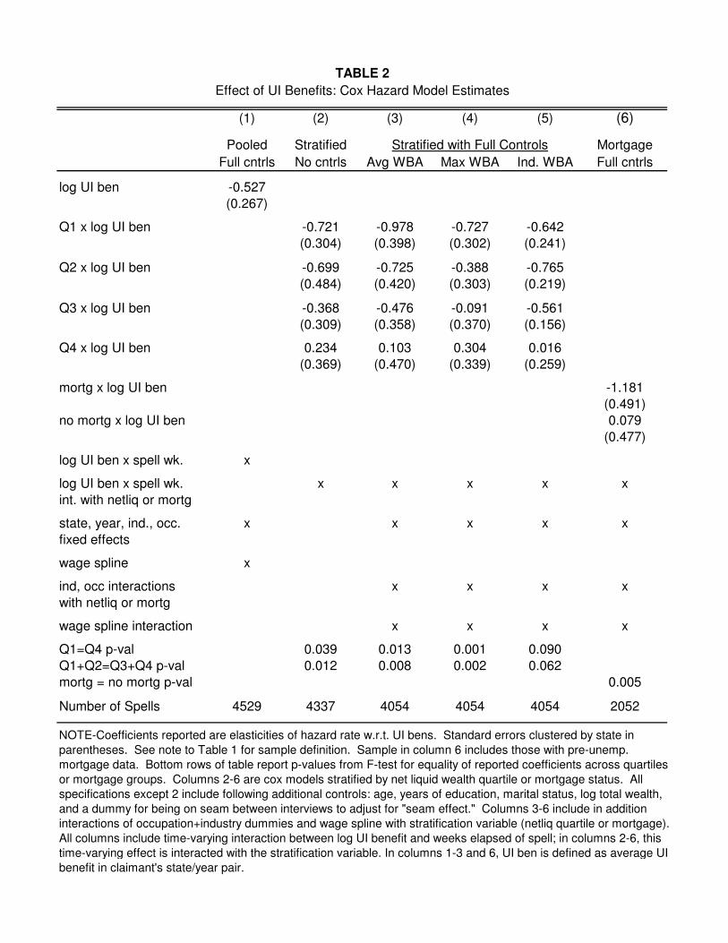
(1) (2) (3) (4) (5) (6)

Pooled Stratified Mortgage

Full cntrls No cntrls Avg WBA Max WBA Ind. WBA Full cntrls

log UI ben -0.527

(0.267)

Q1 x log UI ben -0.721 -0.978 -0.727 -0.642

(0.304) (0.398) (0.302) (0.241)

Q2 x log UI ben -0.699 -0.725 -0.388 -0.765

(0.484) (0.420) (0.303) (0.219)

Q3 x log UI ben -0.368 -0.476 -0.091 -0.561

(0.309) (0.358) (0.370) (0.156)

Q4 x log UI ben 0.234 0.103 0.304 0.016

(0.369) (0.470) (0.339) (0.259)

mortg x log UI ben -1.181

(0.491)

no mortg x log UI ben 0.079

(0.477)

log UI ben x spell wk. x

log UI ben x spell wk. x x x x x

int. with netliq or mortg

state, year, ind., occ. x x x x x

fixed effects

wage spline x

ind, occ interactions x x x x

with netliq or mortg

wage spline interaction x x x x

Q1=Q4 p-val 0.039 0.013 0.001 0.090

Q1+Q2=Q3+Q4 p-val 0.012 0.008 0.002 0.062

mortg = no mortg p-val 0.005

Number of Spells 4529 4337 4054 4054 4054 2052

TABLE 2

Effect of UI Benefits: Cox Hazard Model Estimates

Stratified with Full Controls

NOTE-Coefficients reported are elasticities of hazard rate w.r.t. UI bens. Standard errors clustered by state in

parentheses. See note to Table 1 for sample definition. Sample in column 6 includes those with pre-unemp.

mortgage data. Bottom rows of table report p-values from F-test for equality of reported coefficients across quartiles

or mortgage groups. Columns 2-6 are cox models stratified by net liquid wealth quartile or mortgage status. All

specifications except 2 include following additional controls: age, years of education, marital status, log total wealth,

and a dummy for being on seam between interviews to adjust for "seam effect." Columns 3-6 include in addition

interactions of occupation+industry dummies and wage spline with stratification variable (netliq quartile or mortgage).

All columns include time-varying interaction between log UI benefit and weeks elapsed of spell; in columns 2-6, this

time-varying effect is interacted with the stratification variable. In columns 1-3 and 6, UI ben is defined as average UI

benefit in claimant's state/year pair.

Pooled No Severance Severance

(0.81) (0.19)

Prior to or at job loss:

Mean annual wage $28,149 $26,213 $37,174

Median annual wage $20,848 $19,347 $30,693

Age 36.2 35.2 40.6

Percent dropouts 14% 15% 6%

Percent college grads 17% 13% 34%

Percent married 58% 56% 68%

Mean job tenure (years) 4.5 3.8 8.1

Median job tenure (years) 1.9 1.5 4.8

Post-layoff:

Weekly unemployment benefits $198 $190 $236

Replacement Rate 49% 51% 43%

Mean unemployment duration 24.3 24.0 25.6

Median unemployment duration 20.0 20.0 22.0

Mean compensated duration 15.8 15.3 18.2

Median compensated duration 16.0 16.0 20.0

NOTE--Table entries are means unless otherwise noted. Data are from surveys of job losers

conducted by Mathematica. Sample includes prime-age male UI claimants who are not on temporary

layoff. Pooled sample size is 2,441 observations. See Appendix C for details. Data is reweighted

using sampling probabilities to yield estimates for a representative sample of job losers. Pre-unemp

job tenure is number of years spent working at firm from which worker was laid off. Weekly

unemployment benefit is actual individual benefit based on UI records. Replacement rate is weekly

benefit times 52 divided by annual wage. Unemployment duration is time elapsed from end of last job

to start of next job. Compensated duration is weeks of UI collected. All monetary values are in real

1990 dollars.

TABLE 3

Summary Statistics by Severance Receipt for Mathematica Sample

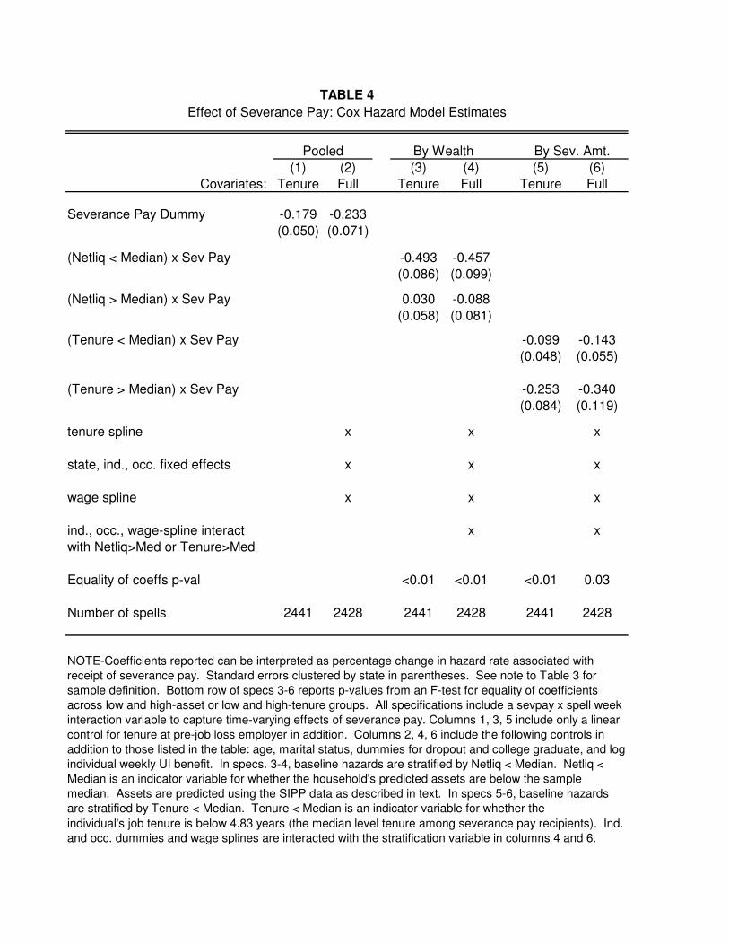
(1) (2) (3) (4) (5) (6)

Covariates: Tenure Full Tenure Full Tenure Full

Severance Pay Dummy -0.179 -0.233

(0.050) (0.071)

(Netliq < Median) x Sev Pay -0.493 -0.457

(0.086) (0.099)

(Netliq > Median) x Sev Pay 0.030 -0.088

(0.058) (0.081)

(Tenure < Median) x Sev Pay -0.099 -0.143

(0.048) (0.055)

(Tenure > Median) x Sev Pay -0.253 -0.340

(0.084) (0.119)

tenure spline x x x

state, ind., occ. fixed effects x x x

wage spline x x x

ind., occ., wage-spline interact x x

with Netliq>Med or Tenure>Med

Equality of coeffs p-val <0.01 <0.01 <0.01 0.03

Number of spells 2441 2428 2441 2428 2441 2428

TABLE 4

Effect of Severance Pay: Cox Hazard Model Estimates

individual's job tenure is below 4.83 years (the median level tenure among severance pay recipients). Ind.

and occ. dummies and wage splines are interacted with the stratification variable in columns 4 and 6.

NOTE-Coefficients reported can be interpreted as percentage change in hazard rate associated with

receipt of severance pay. Standard errors clustered by state in parentheses. See note to Table 3 for

sample definition. Bottom row of specs 3-6 reports p-values from an F-test for equality of coefficients

across low and high-asset or low and high-tenure groups. All specifications include a sevpay x spell week

interaction variable to capture time-varying effects of severance pay. Columns 1, 3, 5 include only a linear

control for tenure at pre-job loss employer in addition. Columns 2, 4, 6 include the following controls in

addition to those listed in the table: age, marital status, dummies for dropout and college graduate, and log

individual weekly UI benefit. In specs. 3-4, baseline hazards are stratified by Netliq < Median. Netliq <

Median is an indicator variable for whether the household's predicted assets are below the sample

median. Assets are predicted using the SIPP data as described in text. In specs 5-6, baseline hazards

are stratified by Tenure < Median. Tenure < Median is an indicator variable for whether the

Pooled By Wealth By Sev. Amt.

Figure 1

UI Benefit and Liquidity Effects by Initial Assets

Benefit or Annuity Level (a,b)

Pro

ba

bili

ty o

f fin

din

g a

jo

b in

peri

od

0 (

s0)

s0(a;A0= -$1000)

s0(b;A0=-$1000)s0(a;A0=$13,000)

s0(b,A0=$13,000)

NOTE–This figure plots simulated values of period 0 search intensity (s0) for two agents, one with

A0 = −$1000 and the other with A0 = $13, 000. Model is parametrized as follows:

utility uc = vc = c1−γ

1−γ with γ = 1. 75; disutility of search ψs = θ s1+κ

1+κ for s ≤ 0. 25;.ψs = ∞ for

s > 0. 25 with κ = 0. 1, θ = 5; wage w = $340 per week, asset limit L = −$1000, T = 500; UI benefit

bt = b for t ≤ 25, bt = 0 for t > 25; annuity payment at = 0. 25w + a for t ≤ 25 and at = 0. 25w for

t > 25. Solid curves plot s0 as a function of UI benefit level b, ranging from b = 0. 05w = $17 per week to

b = 0. 95w = $323 per week, holding fixed a = 0. Dashed curves plot s0 as a function of an increment in

the annuity over the first 26 weeks, holding fixed b = 0.

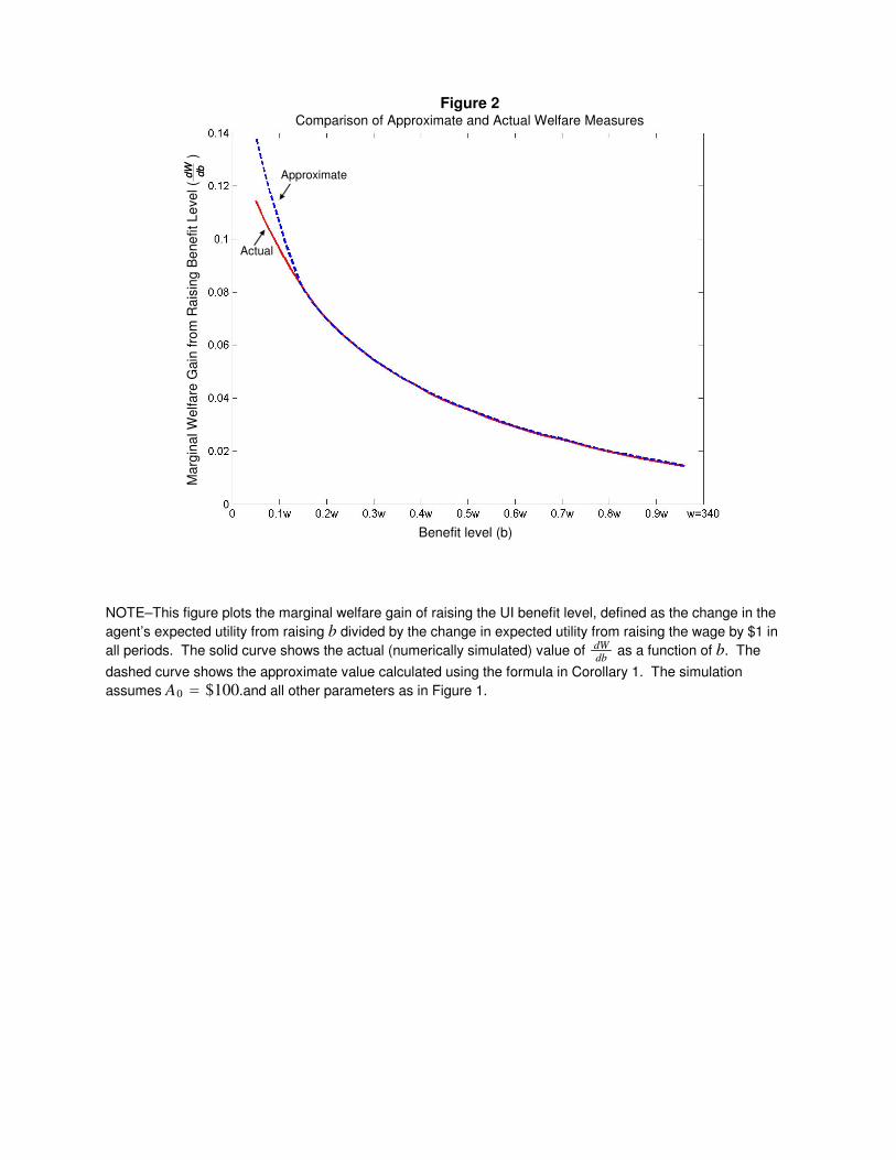
Figure 2

Comparison of Approximate and Actual Welfare Measures

Benefit level (b)

Ma

rgin

al W

elfa

re G

ain

fro

m R

ais

ing

Be

ne

fit L

eve

l (

)

Approximate

Actual

dW

db

dW

db

NOTE–This figure plots the marginal welfare gain of raising the UI benefit level, defined as the change in the

agent’s expected utility from raising b divided by the change in expected utility from raising the wage by $1 in

all periods. The solid curve shows the actual (numerically simulated) value of dW

dbas a function of b. The

dashed curve shows the approximate value calculated using the formula in Corollary 1. The simulation

assumes A0 = $100.and all other parameters as in Figure 1.

.2.4

.6.8

1

Fra

ctio

n U

nem

plo

yed

0 10 20 30 40 50Weeks Unemployed

Avg. UI benefit below mean Avg. UI benefit above mean

Effect of UI Benefits on Durations: Lowest Quartile of Net Wealth

Figure 3a

Mean rep. rate = .53

Mean rep. rate = .48

Wilcoxon Test for Equality: p = 0.01

.2.4

.6.8

1

Fra

ctio

n U

nem

plo

yed

0 10 20 30 40 50Weeks Unemployed

Avg. UI benefit below mean Avg. UI benefit above mean

Effect of UI Benefits on Durations: Second Quartile of Net Wealth

Figure 3b

Mean rep. rate = .48

Mean rep. rate = .53

Wilcoxon Test for Equality: p = 0.04

NOTE–Sample for both figures consists of observations in the core SIPP sample for which pre-unemployment

wealth data are available. See Table 1 for definition of core sample and definition of net liquid wealth. Figure

3a includes households in lowest quartile of real net liquid wealth. Figure 3b includes those in second quartile.

Each figure plots Kaplan-Meier survival curves for two groups of individuals: those in state/year pairs with

average weekly benefit amounts (WBA) below the sample mean and those in state/year pairs with WBAs

above the mean. The mean replacement rate is the average individual-level predicted benefit divided by wage

for observations in the relevant group. Survival curves are adjusted for seam effect by fitting a Cox model with

seam dummy and recovering baseline hazards.

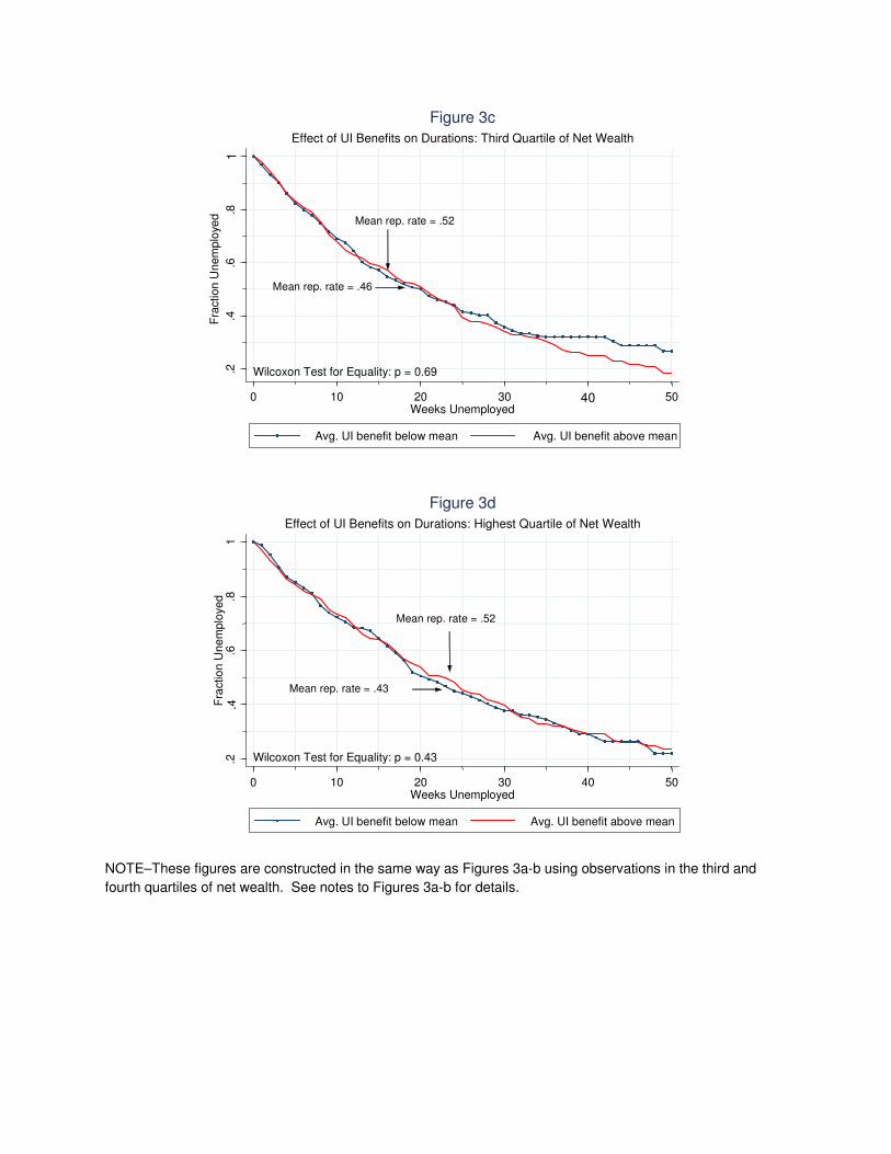
.2.4

.6.8

1

Fra

ctio

n U

nem

plo

yed

0 10 20 30 40 50Weeks Unemployed

Avg. UI benefit below mean Avg. UI benefit above mean

Effect of UI Benefits on Durations: Third Quartile of Net Wealth

Figure 3c

Mean rep. rate = .46

Mean rep. rate = .52

Wilcoxon Test for Equality: p = 0.69

.2.4

.6.8

1F

ract

ion U

nem

plo

yed

0 10 20 30 40 50Weeks Unemployed

Avg. UI benefit below mean Avg. UI benefit above mean

Effect of UI Benefits on Durations: Highest Quartile of Net Wealth

Figure 3d

Mean rep. rate = .43

Mean rep. rate = .52

Wilcoxon Test for Equality: p = 0.43

NOTE–These figures are constructed in the same way as Figures 3a-b using observations in the third and

fourth quartiles of net wealth. See notes to Figures 3a-b for details.

.2.4

.6.8

1F

ract

ion U

nem

plo

yed

0 10 20 30 40 50Weeks Unemployed

Avg. UI benefit below mean Avg. UI benefit above mean

Effect of UI Benefits on Durations: Households with Mortgages

Figure 4a

Wilcoxon Test for Equality: p = 0.01

Mean rep. rate = .52

Mean rep. rate = .45

.2.4

.6.8

1F

ract

ion U

nem

plo

yed

0 10 20 30 40 50Weeks Unemployed

Avg. UI benefit below mean Avg. UI benefit above mean

Effect of UI Benefits on Durations: Households without Mortgages

Figure 4b

Wilcoxon Test for Equality: p = 0.31

Mean rep. rate = .47

Mean rep. rate = .53

NOTE–These figures are constructed in the same way as Figures 3a-b; see notes to Figures 3a-b for

additional details. Figure 4a includes households who make mortgage payments; 4b includes all others. Only

observations with mortgage data prior to job loss are included.

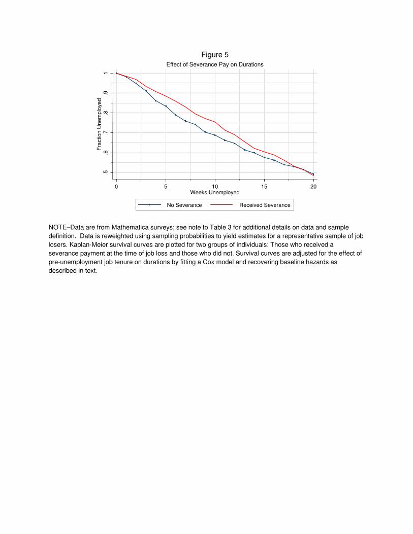
.5.6

.7.8

.91

Fra

ctio

n U

ne

mplo

yed

0 5 10 15 20Weeks Unemployed

No Severance Received Severance

Effect of Severance Pay on Durations

Figure 5

NOTE–Data are from Mathematica surveys; see note to Table 3 for additional details on data and sample

definition. Data is reweighted using sampling probabilities to yield estimates for a representative sample of job

losers. Kaplan-Meier survival curves are plotted for two groups of individuals: Those who received a

severance payment at the time of job loss and those who did not. Survival curves are adjusted for the effect of

pre-unemployment job tenure on durations by fitting a Cox model and recovering baseline hazards as

described in text.

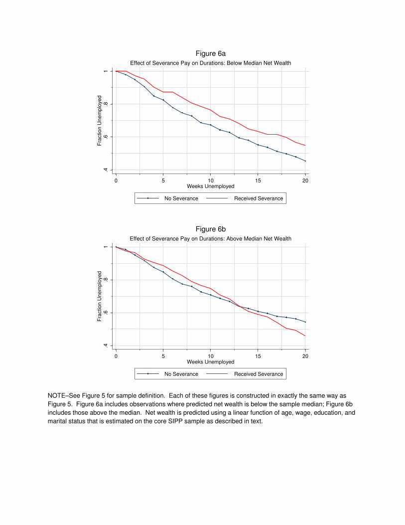
.4.6

.81

Fra

ctio

n U

nem

plo

yed

0 5 10 15 20Weeks Unemployed

No Severance Received Severance

Effect of Severance Pay on Durations: Below Median Net Wealth

Figure 6a

.4.6

.81

Fra

ction

Un

em

plo

yed

0 5 10 15 20Weeks Unemployed

No Severance Received Severance

Effect of Severance Pay on Durations: Above Median Net Wealth

Figure 6b

NOTE–See Figure 5 for sample definition. Each of these figures is constructed in exactly the same way as

Figure 5. Figure 6a includes observations where predicted net wealth is below the sample median; Figure 6b

includes those above the median. Net wealth is predicted using a linear function of age, wage, education, and

marital status that is estimated on the core SIPP sample as described in text.

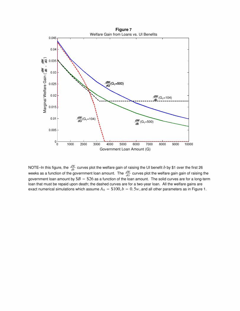
Government Loan Amount (G)

Marg

ina

l W

elfare

Gain

(

,

)

Figure 7

Welfare Gain from Loans vs. UI Benefits

(GT=104)

(GT=500)(GT=104)

dW

db

dW

db

dW

db

dW

db

dW

db

dW

db

(GT=500)dW

dG(GT=500)dW

dG

dW

dG

dW

dG

dW

dG

dW dG

dW dG

NOTE–In this figure, the dW

dbcurves plot the welfare gain of raising the UI benefit b by $1 over the first 26

weeks as a function of the government loan amount. The dW

dGcurves plot the welfare gain gain of raising the

government loan amount by $B = $26 as a function of the loan amount. The solid curves are for a long-term

loan that must be repaid upon death; the dashed curves are for a two-year loan. All the welfare gains are

exact numerical simulations which assume A0 = $100, b = 0. 5w,.and all other parameters as in Figure 1.