NBER WORKING PAPER SERIES

CREDIT MARKET CONSEQUENCES OF IMPROVED PERSONAL IDENTIFICATION:FIELD EXPERIMENTAL EVIDENCE FROM MALAWI

Xavier GinéJessica Goldberg

Dean Yang

Working Paper 17449http://www.nber.org/papers/w17449

NATIONAL BUREAU OF ECONOMIC RESEARCH1050 Massachusetts Avenue

Cambridge, MA 02138September 2011

This paper was previously circulated under the title “Identification Strategy: A Field Experiment onDynamic Incentives in Rural Credit Markets.” Santhosh Srinivasan deserves the highest accoladesfor top-notch field work management and data collection. Lutamyo Mwamlima and Ehren Foss werekey contributors to the success of the field work, and Niall Keleher helped organize wrap-up data entry.We appreciate the vital support and assistance of Michael Carter, Charles Chikopa, Sander Donker,Lena Heron, Weston Kusani, David Rohrbach, Kondwani Shaba, Mark Visocky, and Eliza Waters.We received excellent comments from Abhijit Banerjee, Martina Björkman, Shawn Cole, Alan deBrauw, Quy-Toan Do, Greg Fischer, Raj Iyer, Dean Karlan, Craig McIntosh, Dilip Mookherjee, JonathanMorduch, John Papp, Jean Philippe Platteau, Mark Rosenzweig, and participants at presentations atBocconi U., U. Maryland, U. Michigan, U. Malawi, U. Namur, Oxford U., Syracuse U., UCLA, UCSan Diego’s 2009 microfinance conference, SITE 2009 at Stanford, NEUDC 2009 at Tufts, the 3rdImpact Evaluation Network conference (2009) in Bogota, and BREAD 2010 in Montreal. This projectwas funded by the World Bank Research Committee, USAID’s BASIS AMA CRSP, and USAID Malawi.The views expressed herein are those of the authors and do not necessarily reflect the views of theNational Bureau of Economic Research.

NBER working papers are circulated for discussion and comment purposes. They have not been peer-reviewed or been subject to the review by the NBER Board of Directors that accompanies officialNBER publications.

© 2011 by Xavier Giné, Jessica Goldberg, and Dean Yang. All rights reserved. Short sections of text,not to exceed two paragraphs, may be quoted without explicit permission provided that full credit,including © notice, is given to the source.

Credit Market Consequences of Improved Personal Identification: Field Experimental Evidencefrom MalawiXavier Giné, Jessica Goldberg, and Dean YangNBER Working Paper No. 17449September 2011JEL No. O12,O16

ABSTRACT

We report the results of a randomized field experiment that examines the credit market impacts ofimprovements in a lender's ability to determine borrowers’ identities. Improved personal identificationenhances the credibility of a lender’s dynamic repayment incentives by allowing it to withhold futureloans from past defaulters and expand credit for good borrowers. The experimental context, rural Malawi,is characterized by an imperfect identification system. Consistent with a simple model of borrowerheterogeneity and information asymmetries, fingerprinting led to substantially higher repayment ratesfor borrowers with the highest ex ante default risk, but had no effect for the rest of the borrowers. Thechange in repayment rates is driven by reductions in adverse selection (smaller loan sizes) and lowermoral hazard (for example, less diversion of loan-financed fertilizer from its intended use on the cashcrop).

Xavier GinéThe World Bankxgine@worldbank.org

Jessica GoldbergUniversity of MarylandDepartment of Economics3115G Tydings HallCollege Park, MD 20742goldberg@econ.umd.edu

Dean YangUniversity of MichiganGerald R. Ford School of Public Policyand Department of Economics735 S. State Street, Room 3316Ann Arbor, MI 48109and NBERdeanyang@umich.edu

1

1. Introduction

Imperfections in credit markets are widely seen as key barriers to growth (King and

Levine, 1993). Among such imperfections, asymmetric information problems play a prominent

role, as they limit the ability of borrowers to commit to carrying out their obligations under debt

contracts. Borrowers cannot credibly reveal their borrower type (adverse selection), promise to

exert sufficient effort on their enterprises (ex-ante moral hazard), or promise to repay loans upon

realization of enterprise profits, even when such profits are sufficient for repayment (ex-post

moral hazard).1 Lenders seek to mitigate asymmetric information problems by imposing

collateral requirements, engaging in costly screening of borrowers prior to approval, and – when

a credit reporting system is available – sharing credit information with other lenders. Microcredit

institutions have addressed informational problems by relying on non-traditional mechanisms

such as group liability. However, microlenders have recently come under attack, especially in

India, because of allegations of over-indebtedness of clients driven in part by rapid growth and

increased competition. As a result, microlenders are seeking to participate in credit bureaus,

much like traditional lenders.2

For a credit bureau to function effectively, however, it must be possible to uniquely

identify individuals with reasonable certainty. Identification is necessary in order to retrieve a

current loan applicant’s past credit history from a credit database. Most developed countries have

a unique identification system in the form of a social security number or government-issued

photo identification. But in many of the world’s poorer countries, large segments of the

population lack formal identification documents, and even for those who have them, there is

often no national system for uniquely identifying individuals in a database. In these countries,

lenders accept different forms of identification, such as a passport, a health insurance policy

number or even a letter from the local village leader. Because documents can be falsified, and

because individuals may simply use different types of identification when dealing with different

lenders, it is extremely difficult to track a customer across multiple lenders, and it can even be

difficult for lenders to identify defaulters within their own client base. Loan defaulters may avoid

sanction for past default by simply applying for new loans under different identities.

1 For reviews of this literature, see Ghosh, Mookherjee and Ray (2000), and Conning and Udry (2005). 2 One of the recommendations of the Malegam Committee, set up in October 2010 after the crisis in Andhra Pradesh, India, was the establishment of a credit bureau and the adoption of a customer protection code.

2

Lenders respond by limiting the supply of credit, due to the inability to sanction

unreliable borrowers and, conversely, to reward reliable borrowers with expanded credit. In rural

areas, the result is that smallholder farmers are severely constrained in their ability to finance

crucial inputs such as fertilizer and improved seeds, which limits production of both subsistence

and cash crops.

Motivated by the benefits of a unique identification system, a number of efforts in the

developing world are underway, many on a massive scale. For example, the Indian government

has embarked on a vast effort to fingerprint and assign personal identification numbers that will

replace all other forms of identification and enable citizens to access credit markets, public

services and subsidies on food, energy and education that now suffer from major pilferage

(Planning Commission, 2005; The Economist, 2011; Polgreen, 2011).

Despite its importance, there is essentially no empirical evidence thus far on the impacts

of improved personal identification in credit markets. A number of questions are of general

interest. First, how do improvements in personal identification affect borrower and lender

behavior and ultimately loan repayment rates? Second, how prevalent are adverse selection and

moral hazard in the credit market? And finally, how does improved personal identification affect

the operation of credit bureaus?

We report the results from a randomized field experiment that sheds light on the above

questions. The experiment randomizes fingerprinting of loan applicants to test the impact of

improved personal identification. The experiment was carried out in a context—rural Malawi—

characterized by an imperfect identification system and limited access to credit.

According to the 2006 Doing Business Report, Malawi ranked 109 out of 129 countries

in terms of private credit to GDP, a frequently-used measure of financial development. Malawi

also gets the lowest marks in the “depth of credit information index” which proxies for the

amount and quality of information about borrowers available to lenders. Few rural Malawian

households have access to loans for production purposes: only 11.7% report any production

loans in the past 12 months, and among these loans only 40.3% are from formal lenders.3

In the experiment, farmers who applied for agricultural input loans to grow paprika were

randomly assigned to either 1) a control group, or 2) a treatment group where each member had a

3 Figures are nationally representative and come from the 2004 Malawi Integrated Household Survey. Formal lenders include commercial banks, NGOs and microfinance institutions; informal lenders include moneylenders, family, and friends.

3

fingerprint collected as part of the loan application. A key advantage of fingerprints as a form of

personal identification is that they are unique to and embodied in each person, so they cannot be

forgotten, lost or stolen. Improved borrower identification allows lenders to construct accurate

credit histories and condition future lending on past repayment performance. Loan repayment

could improve with fingerprinting, by making the lender’s threats of future credit denial as well

as promises of larger future loans more credible.

To frame the empirics, we develop a simple two-period model in the spirit of Stiglitz and

Weiss (1983) that incorporates both adverse selection and moral hazard and show that dynamic

incentives (that is, the ability to deny credit in the second period based on the first period

repayment performance), can reduce both types of asymmetric information problems and

therefore raise repayment. Adverse selection problems can be mitigated because riskier

individuals that would otherwise default may now take out smaller loans (or avoid borrowing

altogether) to ensure access to credit in the future.4 In addition, borrowers may have greater

incentives to ensure that agricultural production is successful, either by exerting more effort or

by diverting fewer resources away from production (lower moral hazard). Also, intuitively, the

model predicts that the impact of dynamic incentives on borrowing, farmer actions during the

production phase, and repayment will be largest for the riskiest individuals.

We find that fingerprinting led to substantially higher repayment rates for the subgroup of

borrowers with the highest ex-ante default risk.5 In the context of the model, this result suggests

that fingerprinting, by improving personal identification, enhanced the credibility of the lender’s

dynamic incentive. The impact of fingerprinting on repayment in the highest default risk

subgroup (representing 20% of borrowers) is large: the average share of the loan repaid (two

months after the due date) was 66.7% in the control group, compared to 92.2% among

fingerprinted borrowers.6 In other words, for these farmers fingerprinting accounts for roughly

4 In this paper we use the term “adverse selection” to mean ex-ante selection effects deriving from borrowers’ hidden information. We acknowledge that such selection may occur on the basis of either unobserved risk type (emphasized in the model) or unobserved anticipated effort (as highlighted by Karlan and Zinman, 2009). 5 To create the ex-ante default risk measure, we regress loan repayment rates on borrowers’ baseline characteristics in the control group, and then predict loan repayment for the entire sample (including the treatment group). This essentially creates a “credit score” for each borrower based on their ex-ante (pre-borrowing) characteristics. We provide further details on this procedure in Section 4. 6 The treatment effect implied by these figures is not regression-adjusted, but regression-based estimates are (as would be expected) very similar.

4

three-quarters of the gap between repayment in the control group and full repayment. By

contrast, fingerprinting had no impact on repayment for farmers with low ex ante default risk.

While we cannot separate the effects of moral hazard and adverse selection on

repayment, we collect unique additional evidence that points to the presence of both

informational problems. Fingerprinting leads farmers to choose smaller loan sizes. In the context

of the theoretical model, this is consistent with a reduction in adverse selection. In addition, high-

default-risk farmers who are fingerprinted also divert fewer inputs away from the contracted crop

(paprika), which in the model represents a reduction in moral hazard. When we compare these

benefits to estimated costs of implementation, we find that adoption of fingerprinting is cost-

effective, with a benefit-cost ratio of 2.34.7

The key contribution of the paper, in our view, is that it provides the first empirical

evidence of the importance of personal identification for credit market efficiency. Imperfect

personal identification is an information problem that has received little attention in the

literature. Prior to this study, the extent to which identification of borrowers is a problem for

formal lenders – in any sample population – was unknown. Our results indicate that alleviating

this specific information asymmetry in rural Malawi has non-negligible benefits for credit

markets.

Our analysis is further distinguished by the nature of our outcome data. In addition to

using the lender’s administrative data to measure impacts on borrowing decisions and

repayment, we also use a detailed follow-up survey to estimate impacts on several typically

unobserved behaviors related to moral hazard. For example, we provide direct evidence of

changes in production decisions and the use of borrowed funds stemming from improved

identification.

This paper also has implications for the perceived benefits of a credit reporting system.

Despite the absence of a credit bureau in Malawi, study participants were told that their

fingerprints and associated credit histories could be shared with other lenders. Since

fingerprinting led to positive changes in borrower behavior, the paper underscores the borrowers’

belief that improved identification will allow the lender to condition credit decisions on past

7 As we emphasize below, we have used quite conservative implementation cost estimates, often based on our own field implementation costs. The benefit-cost ratio could be even more attractive in a full-scale implementation that spreads fixed costs over a larger volume of borrowers, particularly in the context of a credit bureau with many participating lenders.

5

credit performance. This is important, because it suggests how borrowers may respond to the

introduction of a credit bureau.

A related paper is Karlan and Zinman (2009), henceforth “KZ”, who find experimental

evidence of moral hazard and weaker evidence of adverse selection in urban South Africa. KZ

introduce a dynamic incentive by making future interest rates conditional on current loan

repayment. Our experiment differs from KZ’s in several key ways. First, our experiment

manipulates the credibility of dynamic incentives, while KZ’s experiment informs borrowers of

the existence of a dynamic incentive. Second, our follow-up survey provides insight into the

specific behaviors that the intervention affects and that result in higher repayment. KZ, by

contrast, relies only on the lender’s administrative data and so cannot shed light on what

borrower behaviors may have changed. Third, the timing of our intervention relative to the

borrowing decision differs. In KZ, the dynamic incentive is announced after clients have agreed

to borrow (and all loan terms have been finalized), so differences in repayment can only be due

to moral hazard. In our case, the intervention that improves dynamic incentives is revealed

before agents decide to borrow. This makes it possible to examine changes in the composition of

borrowers and in loan size. In addition, we estimate the more relevant policy parameter because

potential borrowers cannot be repeatedly surprised.

We informed the lender which clubs had been fingerprinted, so the lender could have

changed its behavior towards treated and control clubs. For example, loan officers could have

spent more time to monitoring and enforcing repayment from control clubs, since treatment clubs

were already subject to dynamic incentives. We provide evidence to the contrary: approval

decisions and monitoring of clubs by loan officers did not differ across treated and control clubs.

We therefore interpret our findings as emerging solely from borrowers’ responses.

By documenting impacts on behaviors related to adverse selection and moral hazard, our

findings contribute to a burgeoning empirical literature that tests claims made by contract theory

and measures the prevalence of asymmetric information (see Chiappori and Salanie, 2003 for a

review). A number of recent papers provide empirical evidence of the existence and impacts of

asymmetric information in credit markets, in both developed and developing countries. Ausubel

(1999) uses a large-scale randomized trial of direct-mail pre-approved solicitations from a major

US credit card company and finds evidence of higher risk individuals selecting less favorable

credit cards, consistent with adverse selection. Klonner and Rai (2009) exploit the introduction

6

of a cap in bidding roscas of South India and find higher repayment rates in earlier rounds

attributable to changes in the composition of bidders, consistent with lower adverse selection.

Visaria (2009) documents the positive impact of expedited legal proceedings on loan repayment

among large Indian firms, even among loans that originated before the reform, consistent with a

reduction in moral hazard. Giné and Klonner (2005) find that incomplete information about

fishermen’s ability in coastal India limits their access to credit for technology adoption. Edelberg

(2004) also develops a model of adverse selection and moral hazard and finds evidence

consistent with both informational problems in the U.S.8

The paper is also related to a framed experiment conducted by Giné et al. (2010) in Peru

that shows that dynamic incentives can be important. In addition, there is a theoretical and

empirical literature on the impact of credit bureaus that are also related to this paper. The

exchange of information about borrowers should theoretically reduce adverse selection (Pagano

and Jappelli, 1993) and moral hazard (Padilla and Pagano, 2000). Empirically, de Janvry,

McIntosh and Sadoulet (2010) study the introduction of a credit bureau in Guatemala and find

that it did contribute to efficiency in the credit market. The paper is also related to the literature

on the recent rise in personal bankruptcies in the US (Livshits et al. 2010).

The remainder of this paper is organized as follows. Section 2 describes the experimental

design and survey data and Section 3 presents the intuition of a simple model of loan repayment.

Section 4 describes the regression specifications, and Section 5 presents the empirical results.

Section 6 provides additional discussion and robustness checks. Section 7 presents the benefit-

cost analysis of introducing biometric technology, and Section 8 concludes.

2. Experimental design and survey data

The experiment was carried out as part of the Biometric and Financial Innovations in

Rural Malawi (BFIRM) project, a cooperative effort among Cheetah Paprika Limited (CP), the

Malawi Rural Finance Corporation (MRFC), the University of Michigan, and the World Bank.

CP is a privately owned agri-business company established in 1995 that offers extension services

and high-quality inputs to smallholder farmers via an out-grower paprika scheme. MRFC is a

8 Ligon (1998) implements empirical tests of the extent to which consumption allocations can be best described by permanent income, full information, or private information models, and finds that the private information model is most consistent with the data in two out of three ICRISAT villages in India. Paulson, Townsend, and Karaivanov (2006) estimate structurally competing models of credit markets in Thailand and find moral hazard to be important.

7

government-owned microfinance institution and provided financing for the in-kind loan package

for 1/2 to 1 acre of paprika. Loaned funds were not disbursed in cash, but rather took the form of

a credit at an agricultural input supplier for the financed production inputs. For further details on

CP, MRFC, and the loan particulars, please see Online Appendix A.

At the time of the study, the vast majority of farmers in the sample had no access to

formal-sector credit. In our baseline survey, only 6.7% of farmers had any formal loans in the

previous year. Among these few farmers with formal-sector credit, MRFC was the largest single

lender, providing 34% of loans (more than twice the share of the next largest lender).9 Farmers

therefore had a strong interest in maintaining good credit history with MRFC so as to maintain

access to what would likely be their primary source of formal credit in the future.

In the absence of fingerprinting, farmer identification relies on the personal knowledge of

loan officers. Loan officers do build up knowledge of borrowers over time, which allows MRFC

to implement some dynamic incentives: it does attempt to withhold loans from past defaulters,

and to reward reliable borrowers with increased loan amounts at lower interest rates. However,

the identification “technology” based on personal loan officer knowledge is regarded as

imperfect by top management at MRFC, who view the existing dynamic incentives as weak.10

Loan officers are sometimes promoted and rotated to other localities. Among the 11 loan officers

who were responsible for our study participants, the median number of years at the branch is

only two, while the median number of years working for the lender is 13.11 In the absence of an

independent mechanism for identifying borrowers, the institutional memory is lost when the loan

officer is transferred to another location. Even when loan officers remain in a given location over

time, the large number of borrowers can lead them to make mistakes in identification. In this

project, loan officers issued an average of 104 loans, and also handled other loan customers not

associated with the project. Loan officers may also rely for identification on local informants,

9 Across study areas, access to formal credit varies from 4% to 10%. In Dedza, the region with highest access to formal loans, MRFC provides almost half of these formal loans. 10 While we do not have systematic evidence on past defaulters taking out new loans under false identities, an accumulation of anecdotes had convinced top management at MRFC and other institutions that this was a major obstacle in their effort to expand access to credit. 11 Because soft information about borrowers is important, one may be surprised by the high loan officer turnover rate. MRFC, like other lenders, rotates credit officers for many reasons. For example, rotation is thought to improve morale and help minimize corruption. Promotion of successful individuals within the organization also leads to replacement of loan officers at the local level and some loss of soft information on borrowers.

8

local leaders, and other borrowing group members, but such methods are also imperfect because

of the possibility of collusion against the lender among fellow villagers.

The timeline of the experiment is presented in Appendix Figure 1. Our study sample

consists of 214 clubs with 3,206 farmers in Dedza, Mchinji, Dowa and Kasungu districts. Farmer

clubs in the study were randomly assigned to be fingerprinted (the treatment group) or not (the

control group), with an equal probability of being in either group. Randomization of treatment

status was carried out after stratifying by locality and week of club visit.12 Each loan officer is

assigned to one locality. The stratification by locality and week of club visit thus ensured

stratification by loan officer as well (i.e., each loan officer was responsible for roughly the same

number of treatment and control clubs).

Club visits began with private administration of the baseline survey to individual farmers,

and were followed by a training session. Both treatment and control groups were given a

presentation on the importance of credit history in ensuring future access to credit. The training

emphasized that defaulters would face exclusion from future borrowing, while borrowers in good

standing could be rewarded with larger loans in the future. Then, in treatment clubs only,

individual participants’ fingerprints were collected. Our project staff explained how their

fingerprint uniquely identified them for credit reporting to all major Malawian rural lenders, and

that future credit providers would be able to access the applicant’s credit history simply by

checking his or her fingerprint.13 Online Appendix A provides the script used during the training.

See Online Appendix B for further technical details on the biometric technology used.

After fingerprints were collected, a demonstration program was used to show participants

that the computer was now able to identify an individual with only a fingerprint. One farmer was

chosen at random to have his right thumb re-scanned, and the club was shown that the person’s

name and demographic information (entered earlier alongside the original fingerprint scan) was

retrieved by the computer program. During these demonstration sessions all farmers whose

fingerprints were re-scanned were correctly identified. The control group was not fingerprinted,

12 In other words, each unique combination of locality and week of initial club visit constituted a stratification cell, within which clubs were evenly divided randomly between treatment and control (or as close as possible to evenly divided, when there was an odd number of clubs in the stratification cell). There are 11 localities in the study, each of which was covered by one loan officer. The full sample of 214 clubs (3,206 farmers) was spread across 31 stratification (location-week) cells. 13 Our team of enumerators encountered essentially no opposition to fingerprint collection.

9

but as mentioned previously, also received the same training emphasizing the importance of

one’s credit history and how it influences one’s future credit access.14

The baseline survey administered prior to the training and the collection of fingerprints

included questions on individual demographics (education, household size, religion), income

generating activities and assets including detailed information on crop production and crop

choice, livestock and other assets, risk preferences, past and current borrowing activities, and

past variability of income. Summary statistics from the baseline survey are presented in Table 1,

and variable definitions are provided in Online Appendix C.15

After the completion of the survey, credit history training, and fingerprinting of the

treatment group, the names and locations of the members that applied for loans along with their

treatment status were handed over to MRFC loan officers so that they could screen and approve

the clubs according to their protocols. Among other standard factors, MRFC conditions lending

on the club’s successful completion of 16 hours of training. MRFC approved loans for 2,063 out

of 3,206 customers (in 121 out of 214 clubs). Of the customers approved for loans, some failed

to raise the required down payment and others opted not to borrow for other reasons. The

sample of borrowers consists of 1,147 loan customers from 85 clubs, in 21 stratification

(location-week) cells.16 Loan packages had an average value of MK 16,913 (US$117).17

Within a group, take-up of the loan was an individual decision, but the subset of farmers

who took up the loan was told that they were jointly liable for each others’ loans. In practice,

however, joint liability at this lender was not enforced. MRFC applies sanctions primarily on

individual defaulters and not on other (non-defaulting) members of a borrowing group. In other

words, an individual who repaid a previous loan could obtain a new loan even if other borrowers

in the same group had failed to repay a past loan, as long as defaulters from the group were

removed before the group applied for new loans.

14 Because we provided education on the importance of credit history to our control group as well, we can estimate neither the impact of fingerprinting without such education, nor the impact of the credit history education alone. 15 To ensure that survey answers were not influenced by knowledge of the experiment or the respondent’s treatment status, survey data were collected prior to the credit history education and fingerprinting intervention. 16 While a natural question at this point is whether selection into borrowing was affected by treatment status, treatment and control groups did not differ in their rates of MRFC loan approval or the fraction of farmers who ended up with a loan. Furthermore, treated and untreated borrowers do not differ systematically on the basis of baseline characteristics. These points will be discussed in detail in the results section below. 17 All conversions of Malawi kwacha to US dollars in this paper assume an exchange rate of MK145/US$, the average exchange rate at the time of the experiment.

10

During the months of July and August, farmers harvested the paprika crop and sold it to

CP at predefined collection points. CP then transferred the proceeds from the sale to MRFC who

then deducted the loan repayment and credited the remaining post-repayment proceeds to an

individual farmer’s savings account. This garnishing of the proceeds for loan repayment

essentially allows MRFC to “seize” the paprika crop when farmers sell to CP (and for most

farmers it is the only sales outlet).18 Farmers could also make loan repayments directly to MRFC

at their branch locations or during credit officer visits to their villages; this occurred, for

example, among the small number of farmers who sold to paprika buyers other than CP. This

channel of repayment is less desirable to MRFC because it is riskier.

We also implemented a follow-up survey of farmers in August 2008, once crops had been

sold and income received. The sample size of this follow-up survey is 1,226 in total (borrowers

plus non-borrowers), among whom 520 were borrowers.19 The formal loan maturity (payment)

date was September 30, 2008. Some additional payments were made after the formal due date;

MRFC reports that there is typically no additional loan repayment two months past the due date

for agricultural loans. In the empirical analysis we obtain our dependent variables from the

August 2008 survey data as well as administrative data from MRFC on loan take-up, amount

borrowed, and repayment.

Balance of baseline characteristics across treatment vs. control groups

To confirm that the randomization across treatments achieved balance in terms of pre-

treatment characteristics, Online Appendix Table 1 presents the means of several baseline

variables for the control group as reported prior to treatment, alongside the difference vis-à-vis

the treatment group (mean in treatment group minus mean in control group). We also report

statistical significance levels of the difference in treatment-control means. These tests are

presented for both the full baseline sample and the loan recipient sample.

18 Proceeds from other types of crops of course cannot be seized in this way to secure loan repayment because MRFC does not have analogous garnishing arrangements with other crop buyers. 19 The 520 borrowers are spread across 17 stratification (location-week) cells. The follow-up sample is smaller than the sample of baseline borrowers because for budget reasons we could not visit each borrowing household at their place of residence. Instead, we invited study participants to come to a central location at a certain date and time to be administered the follow-up interview. Not all farmers attended the meeting where the follow-up survey was administered, but as we discuss below in Section 5.C. (see Online Appendix Table 3), there is no evidence of selective attrition related to treatment status. For the full sample as well as the borrower subsample, in no regression is fingerprinting or fingerprinting interacted with predicted repayment statistically significantly associated with attrition from the survey.

11

Overall, we find balance between the two groups in both the full baseline sample and the

loan recipient sample. In the full baseline sample, the difference in means for the treatment and

control groups is not significant for any of the 11 baseline variables. In the loan recipient

sample, for 10 out of these 11 baseline variables, the difference in means between treatment and

control groups is not statistically significantly different from zero at conventional levels, and so

we cannot reject the hypothesis that the means are identical across treatment groups. For only

one variable, the indicator for the study participant being male, is the difference statistically

significant (at the 10% level): the fraction male in the treatment group is 6.6 percentage points

lower than in the control group.20

3. A simple model of borrower behavior

Fingerprinting improves the personal identification of borrowers and thus increases the

credibility of dynamic incentives used by the lender. To study how dynamic incentives affect

borrower behavior, Online Appendix D develops a simple model that incorporates both adverse

selection and moral hazard. We provide here an intuitive discussion of the model.

We assume that prospective borrowers have no liquid assets and decide how much to

borrow for cash crop inputs, so the amount invested in production cannot exceed the loan

amount. We introduce adverse selection by assuming that borrowers differ in the probability that

production is successful, while moral hazard is modeled by allowing borrowers to divert the loan

amount instead of investing it in production.21 Consistent with the credit contract offered in the

context of the experiment, we model a lender that offers a loan amount that can take on two

values (depending on the number of fertilizer bags borrowed) and a gross interest rate. We also

assume that when the smaller amount is borrowed, production can cover loan repayment even if

it fails.

When personal identification of clients is not possible, borrowers can obtain a new loan

even if they have defaulted in the past simply by using a different identity. As a result, lenders

20 It turns out, however, that the regression results to come are not substantially affected by the inclusion in the regressions of the “male” indicator and other control variables (results not shown). 21 Given the arrangement to buy the cash crop (paprika) in the experiment, we assume that the lender can only seize cash crop production but not the proceeds from diverted inputs. To be clear, the production of paprika does not reduce moral hazard because paprika faces less production risk than other crops, but rather because it is less risky for the lender, given the lender’s ability to confiscate paprika output for repayment of the loan.

12

are forced to offer the same one-season contract every period, as they cannot tailor the terms of

the contract to individual credit histories.

By contrast, when personal identification is possible, the lender can use dynamic

incentives, conditioning future credit on past repayment performance. In this situation, borrowers

face a tradeoff between diverting inputs away from cash crop production but jeopardizing

chances of a loan in the future versus ensuring repayment of the current loan and therefore

securing a loan in the future. In addition, by choosing the smaller loan amount they obtain lower

net income in the first period in return for securing a loan in the future.

With this setup, the model predicts that dynamic incentives will have different effects on

the optimal choices of borrowers depending on their probability of success. In particular,

borrowers with relatively low probability of success are most affected by the introduction of

dynamic incentives. They choose the higher loan amount and divert it all without dynamic

incentives, but borrow the lower amount and invest it in cash crop production when dynamic

incentives are introduced. Borrowers with the highest probabilities of success are the least

affected: even without dynamic incentives, they never divert inputs and always choose the higher

loan amount. Finally, borrowers with intermediate values of the probability of success will,

upon introduction of dynamic incentives, change either the diversion or the loan size decisions

(depending on parameter values and functional forms).

The model provides a reasonable structure for framing the empirical results to come. Its

key advantage is a close adherence to the context of the experiment, in which the main

simplifying assumptions (e.g., binary loan size and the lender’s inability to seize non-cash-crop

output) are reasonable. That said, our model may not be the only one that could be used to

understand borrower behaviors in this and other contexts; other models may provide a different

interpretation of the results. Therefore, our empirical results should be interpreted in the context

of this specific model.

4. Regression Specification

Because the treatment is assigned randomly at the club level, its impact on the various

outcomes of interest (say, repayment) can be estimated via the following regression equation:

(1) Yijs = + Tjs + s + εijs,

13

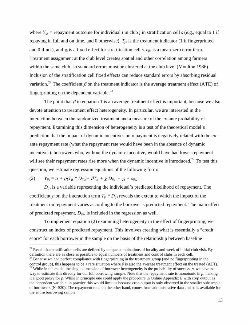
where Yijs = repayment outcome for individual i in club j in stratification cell s (e.g., equal to 1 if

repaying in full and on time, and 0 otherwise), Tjs is the treatment indicator (1 if fingerprinted

and 0 if not), and s is a fixed effect for stratification cell s. εijs is a mean-zero error term.

Treatment assignment at the club level creates spatial and other correlation among farmers

within the same club, so standard errors must be clustered at the club level (Moulton 1986).

Inclusion of the stratification cell fixed effects can reduce standard errors by absorbing residual

variation.22 The coefficient on the treatment indicator is the average treatment effect (ATE) of

fingerprinting on the dependent variable.23

The point that in equation 1 is an average treatment effect is important, because we also

devote attention to treatment effect heterogeneity. In particular, we are interested in the

interaction between the randomized treatment and a measure of the ex-ante probability of

repayment. Examining this dimension of heterogeneity is a test of the theoretical model’s

prediction that the impact of dynamic incentives on repayment is negatively related with the ex-

ante repayment rate (what the repayment rate would have been in the absence of dynamic

incentives): borrowers who, without the dynamic incentive, would have had lower repayment

will see their repayment rates rise more when the dynamic incentive is introduced.24 To test this

question, we estimate regression equations of the following form:

(2) Yijs = + Tjs * Dijs)+ Tjs + Dijs + s + εijs,

Dijs is a variable representing the individual’s predicted likelihood of repayment. The

coefficient on the interaction term Tjs * Dijs reveals the extent to which the impact of the

treatment on repayment varies according to the borrower’s predicted repayment. The main effect

of predicted repayment, Dijs, is included in the regression as well.

To implement equation (2) examining heterogeneity in the effect of fingerprinting, we

construct an index of predicted repayment. This involves creating what is essentially a “credit

score” for each borrower in the sample on the basis of the relationship between baseline 22 Recall that stratification cells are defined by unique combinations of locality and week of initial club visit. By definition there are as close as possible to equal numbers of treatment and control clubs in each cell. 23 Because we had perfect compliance with fingerprinting in the treatment group (and no fingerprinting in the control group), this happens to be a rare situation where is also the average treatment effect on the treated (ATT). 24 While in the model the single dimension of borrower heterogeneity is the probability of success, p, we have no way to estimate this directly for our full borrowing sample. Note that the repayment rate is monotonic in p, making it a good proxy for p. While in principle one could apply the procedure in Online Appendix E with crop output as the dependent variable, in practice this would limit us because crop output is only observed in the smaller subsample of borrowers (N=520). The repayment rate, on the other hand, comes from administrative data and so is available for the entire borrowing sample.

14

characteristics (some of which may not be observable to the lender) and repayment among

borrowers in the control (non-fingerprinted) group. Limiting the sample to borrowers in the

control group (N=563), we run a regression of repayment (fraction of loan repaid by the

September 30, 2008 due date) on various farmer- and club-level baseline characteristics.

Conceptually, the resulting index will be purged of any bias introduced by effects of

fingerprinting on repayment because it is constructed using coefficients from a regression

predicting repayment for only the control (non-fingerprinted) farmers.

Table 2 presents results from this exercise. Statistically significant results in column 1,

which only includes farmer-level (individual) variables on the right-hand-side, indicates that

older farmers and those who do not self-identify as risk-takers have better repayment

performance on the loan. Inclusion of a complete set of fixed effects for (locality)*(week of

initial club visit) interactions raises the R-squared substantially (from 0.05 in column 1 to 0.46 in

column 2). The explanatory power of the regression is marginally improved further in column 3

(to an R-squared of 0.48) when age and education are specified as categorical variables (instead

of being entered linearly).

We then take the coefficient estimates from column 3 of the table and predict the fraction

of loan repaid for the entire sample (both control and treatment observations). This variable,

which we call “predicted repayment”, is useful for analytical purposes because it is a single

index that incorporates a wide array of baseline information (at the individual and locality level)

correlated with repayment outcomes.25

To investigate heterogeneity in the treatment effect, this index is either interacted linearly

with the treatment indicator (as in equation 2), or it is converted into indicators for quintiles of

the distribution of predicted repayment in the absence of fingerprinting and then interacted with

treatment. For this analysis to be valid, it must be true that randomization leads to balance with

respect to predicted repayment across treatment and control groups. This is indeed what we

find.26 In all regression results where the treatment indicator is interacted with predicted

25 In the loan-recipient subsample, predicted repayment has a mean of 0.79, with standard deviation 0.26. As expected, predicted repayment is highly skewed, with median predicted repayment of 0.90. 26 In regressions of the treatment indicator on the continuous predicted repayment variable and indicators for stratification cells, the coefficient on predicted repayment always far from statistical significance at conventional levels in all samples used in this paper. In regressions of the treatment indicator on indicators for each quintile of repayment, the coefficients on the quintile dummies are individually and jointly insignificantly different from zero in all subsamples.

15

repayment, we report bootstrapped standard errors because the predicted repayment variable is a

generated regressor.27

5. Empirical Results: Impacts of Fingerprinting

This section presents our experimental evidence on the impacts of fingerprinting on a

variety of inter-related outcomes. We examine impacts on loan approval and borrowing

decisions, on repayment outcomes, and on intermediate farmer actions and outcomes that may

ultimately affect repayment.

Tables 3 through 5 will present regression results from estimation of equations (1) and (2)

in a similar format. In each table, each column will present regression results for a given

dependent variable. Panel A will present the coefficient on treatment (fingerprint) status from

estimation of equation (1).

Then, to examine heterogeneity in the effect of fingerprinting, Panels B and C will

present results from estimation of versions of equation (2) where fingerprinting is interacted

linearly with predicted repayment (Panel B) or with dummy variables for quintiles of predicted

repayment (Panel C). In both Panels B and C the respective main effects of the predicted

repayment variables are also included in the regression (but for brevity the coefficients on the

predicted repayment main effects will not be presented). In Panel C, the main effect of

fingerprinting is not included in the regression, to allow each of the five quintile indicators to be

interacted with the indicator for fingerprinting in the regression. Therefore, in Panel C the

coefficient on each fingerprint-quintile interaction should be interpreted as the impact of

fingerprinting on borrowers in that quintile, compared to control group borrowers in that same

quintile.

Finally, in Tables 3 through 5 the mean of the dependent variable in a given column, for

the overall sample as well for each quintile of predicted repayment separately, are reported at the

bottom of each table.

A. Loan approval, take-up, and amount borrowed

27 For coefficients in regressions in the form of equation (2), we calculate standard errors from 200 bootstrap replications. In each replication, we re-sample borrowing clubs from our original data (which preserves the original club-level clustering), compute predicted repayment based on the new sample, and re-run the regression in question using the new value of predicted repayment for that replication. See Efron and Tibshirani (1993) for details.

16

The first key question to ask is whether fingerprinted farmers were more likely to have

their loans approved by the lender, or were more likely to take out loans, compared to the control

group. This question is important because the degree of selectivity in the borrower pool induced

by fingerprinting affects interpretation of any effects on repayment and other outcomes.

Although loan officers were told which clubs had been fingerprinted in September 2007

when loan applications were due, they do not appear to have retained or used this information.

Since biometric technology can be seen as a substitute for loan officer effort, one would expect

loan officers to have better knowledge about non-fingerprinted clubs. However, this is not what

we find. Loan officers’ knowledge about clubs (identity of club officers, number of loans) is not

related to treatment status, and in fact loan officers do not appear to know the treatment status of

clubs. Borrower reports of contact with loan officers are also uncorrelated with treatment. (For

further details on this analysis, see Online Appendix E.) Given that loan officers do not appear to

have responded to the treatment, we interpret impacts of the treatment as emerging solely from

borrowers’ responses to being fingerprinted.

Because loan officers did not take treatment status into account, it is not surprising that

fingerprinting had no effect on loan approval. We also find no effect on loan-take-up by

borrowers, perhaps because clubs were formed with the expectation of credit availability and

fingerprinting did not act as a strong enough deterrent to borrowing to affect farmers’ decisions

at the extensive margin. Columns 1 and 2 of Table 3 present results from estimation of equations

(1) and (2) for the full baseline sample where the dependent variables are, respectively, an

indicator for the lender’s approving the loan for the given farmer (mean 0.63), and an indicator

for the farmer ultimately taking out the loan (mean 0.35).28

There is no evidence that the rate of loan approval or take-up differs substantially across

the treatment and control groups on average: the coefficient on fingerprinting is not statistically

different from zero in either columns 1 or 2, Panel A.

There is also no indication of selectivity in the resulting borrowing pool across subgroups

of borrowers with different levels of predicted repayment. The coefficient on the interaction of

fingerprinting with predicted repayment is not statistically significantly different from zero in

either columns 1 or 2 of Panel B. When looking at interactions with quintiles of predicted

28 Not all farmers who were approved for the loan ended up taking out the loan. Anecdotal evidence indicates that a substantial fraction of non-take-up among approved borrowers resulted when borrowers failed to raise the required deposit (amounting to 15% of the loan amount).

17

repayment (Panel C), while the fingerprint-quintile 2 interaction is positive and significantly

different from zero at the 10% level in the loan approval regression, none of the interaction terms

with fingerprinting are significantly different from zero in the loan take-up regression.

It does appear that, conditional on borrowing, fingerprinted borrowers took out smaller

loans. In Column 3 of Table 3, the dependent variable is the total amount borrowed in Malawi

kwacha. Panel A indicates that loans of fingerprinted borrowers were MK 693 smaller than loans

in the control group on average, a difference that is significant at the 10% level.

The patterns of coefficients in Panel C are suggestive that this effect is confined to

borrowers in the lowest quintile of expected repayment. Differences between fingerprinted and

non fingerprinted borrowers are small and not significant in quintiles two and above, but in

quintile one, where fingerprinted borrowers take out loans that are smaller by MK 2,657 (roughly

US$18) than those in the corresponding quintile in the control group, the difference is marginally

significant (the t-statistic is 1.55).

While the absence of statistical significance in Panel C makes this just a suggestive

result, the pattern is in accord with the theoretical model’s prediction that the “worst” borrowers

(those whose repayment rates would be lowest in the absence of dynamic incentives) will

respond to the imposition of a dynamic incentive by voluntarily reducing their loan sizes.

These results, while only suggestive, are consistent with fingerprinting reducing adverse

selection in the credit market, albeit on a different margin than is usually discussed in the credit

context. Existing research tends to emphasize that improved enforcement should lead low-quality

borrowers to be excluded from borrowing entirely – i.e., the improvement of the borrower pool

operates on the extensive margin. Our results are suggestive that low-quality borrowers choose

smaller loan sizes, which leads the overall loan pool to be less weighted towards low-quality

borrowers. The improvement in the borrowing pool operates on the intensive margin of

borrowing, rather than the extensive margin.

Interpretation of subsequent differences in the repayment rates (discussed below) should

keep this result in mind. Improvements in repayment among fingerprinted borrowers

(particularly among those in the lowest quintile) may in part result from their decisions to take

out smaller loans at the very outset of the lending process and improve their eventual likelihood

of repayment.

B. Loan repayment

18

How did fingerprinting affect ultimate loan repayment? Columns 4-6 of Table 3 present

estimated effects of fingerprinting for the loan recipient sample on three outcomes: outstanding

balance (in Malawi kwacha), fraction of loan paid , and an indicator for whether the loan is fully

paid, all by September 30, 2008 (the official due date of the loan, after which the loan is

officially past due). The next three columns (columns 7-9) are similar, but the three variables

refer to “eventual” repayment as of the end of November 2008. The lender makes no attempt to

collect past-due loans after November of each agricultural loan cycle, so the eventual repayment

variables represent the final repayment status on these loans.

Results for all loan repayment outcomes are similar: fingerprinting improves loan

repayment, in particular for borrowers expected ex ante to have poorer repayment performance.

Coefficients in Panel A indicate that fingerprinted borrowers have lower outstanding balances,

higher fractions paid, and are more likely to be fully paid on-time as well as eventually (and the

coefficients in the regressions for outstanding balance and fraction paid on-time are statistically

significant at the 10% level).

In Panel B, the fingerprinting-predicted repayment interaction term is statistically

significantly different from zero (at the 5% or 1% level) in all regressions. The effect of

fingerprinting on repayment is larger the lower is the borrower’s ex ante likelihood of

repayment. The fingerprint main effect and the “Predicted repayment * fingerprint” interaction

term are jointly significantly different from zero at conventional levels (p-values reported in the

bottom row of the table).

In Panel C, it is evident that the effect of fingerprinting is isolated in the lowest quintile

of expected repayment, with coefficients on the fingerprint-quintile 1 interaction all being

statistically significantly different from zero at the 5% or 1% level and indicating beneficial

effects of fingerprinting on repayment (lower outstanding balances, higher fraction paid, and

higher likelihood of full repayment). Coefficients on other fingerprint-quintile interactions are all

smaller in magnitude and not statistically significantly different from zero (with the exception of

the positive coefficient on the fingerprint-quintile 5 interaction for outstanding balance and the

negative coefficient corresponding interaction term for fraction paid, which is odd and may

simply be due to sampling variation).

The magnitudes of the repayment effect found for the lowest predicted-repayment

quintile are large. The MK7,249.27 effect on eventual outstanding balance amounts to 40% of

19

the average loan size for borrowers in the lowest predicted-repayment quintile. While

outstanding balance should mechanically be lower due to the lower loan size in the lowest

predicted-repayment quintile, the effect is almost three times the size of the reduction in loan

size, so by itself lower loan size cannot explain the treatment effect on repayment. The 32.7

percentage point increase in eventual fraction paid and the 40.8 percentage point increase in the

likelihood of being eventually fully paid are also large relative to bottom quintile percentages of

81% and 68% respectively. Put another way, the fingerprinting-induced increase in repayment

for the lowest quintile accounts for nearly the entire gap between repayment absent

fingerprinting and full repayment.

C. Intermediate outcomes that may affect repayment

In this section we examine decisions that farmers make throughout the planting and

harvest season that may contribute to higher repayment among fingerprinted farmers. The

dependent variables in the remaining results tables are available from a smaller subset of loan

recipients (N=520) who were successfully interviewed in the August 2008 follow-up survey

round. To help rule out the possibility that selection into the 520-observation August 2008

follow-up survey sample might bias the regression results for that sample, Column 2 of Online

Appendix Table 3 examines selection of loan recipients into the follow-up survey sample. The

regressions are analogous in structure to those in the main results tables (Panels A, B, and C),

and the dependent variable is a dummy variable for attrition from the baseline (September 2007)

to the August 2008 survey. There is no evidence of selective attrition related to treatment status:

in no case is fingerprinting or fingerprinting interacted with predicted repayment statistically

significantly associated with attrition from the survey.

Online Appendix Table 4 presents regression results for repayment outcomes that are

analogous to those in columns 4-9 of main Table 3, but where the sample is restricted to this

520-observation sample. The results confirm that the repayment results in the 520-observation

sample are very similar to those in the overall loan recipient sample, in terms of both magnitudes

of effects and statistical significance levels.

Land area allocated to various crops

One of the first decisions that farmers make in any planting season (which typically starts

in November and December) is the proportion of land allocated to different crops. Table 4

examines the average and heterogeneous impact of fingerprinting on land allocation; the

20

dependent variables across columns are fraction of land used in maize (column 1), seven cash

crops (columns 2-8), and all cash crops combined (column 9).29

Why might land allocation to different crops respond to fingerprinting? As discussed in

the context of the theoretical model (footnote 22), non-production of paprika is a form of moral

hazard, since the lender can only feasibly seize paprika output (in collaboration with the paprika

buyer) and not other crops. By not producing paprika (or producing less), the borrower is better

able to avoid repayment. Therefore, by improving the lender’s dynamic incentives, fingerprinting

may discourage such diversion of inputs and land to other crops.

While none of the effects of fingerprinting in Table 4 (either overall in Panel A or in

interaction with predicted repayment in Panels B and C) are statistically significant at

conventional levels, the point estimates provide suggestive evidence that there is an impact of

fingerprinting on land allocation for borrowers in the first predicted-repayment quintile. In this

group, the effect of fingerprinting on land allocated to paprika (column 5, first row of Panel C) is

marginally significant (with a t-statistic of 1.57) and positive, indicating that fingerprinting leads

farmers to allocate 7.7 percentage points more land to paprika. This effect is roughly half the size

of the paprika land allocation in the lowest quintile of predicted repayment.

It is worth considering that the effect on land allocated to paprika may be smaller than it

might be otherwise because farmers began preparing and allocating land earlier in the

agricultural season than our treatment. If land is less easily reallocated than other inputs from

one crop to another, then we would anticipate smaller short run effects on land allocation than on

the use of inputs such as fertilizer and chemicals (to which we now turn). In the long run, when

farmers incorporate the additional cost of default due to fingerprinting into their agricultural

planning earlier in the season, we might find larger impacts on land allocation.

Inputs used on paprika

After allocating land to different crops, the other major farming decision made by farmers

is input application. Non-application of inputs on the paprika crop facilitates default on the loan

and is therefore another form of moral hazard, again since only paprika output can feasibly be

seized by the lender.

It is worth keeping in mind that input application takes place later in the agricultural

cycle than land allocation, and agricultural inputs are more fungible than land. Also, inputs are

29 For each farmer, the values of the variables across columns 1-8 add up to 1.

21

added multiple times throughout the season, so farmers can incorporate new information about

the cost of default into their use of inputs but cannot change land allocation after planting. Thus,

we may expect use of inputs to respond more quickly to the introduction of fingerprinting than

would allocation of land.

Columns 1-7 of Table 5 examine the effect of fingerprinting on the use of inputs on the

paprika crop. The dependent variables in the first 5 columns (all denominated in Malawi

kwacha) are applications of seeds, fertilizer, chemicals, man-days (hired labor), and all inputs

together. Columns 6 and 7 look at, respectively, manure application (denominated in kilograms

because this input is typically produced at home and not purchased) and the number of times

farmers weeded the paprika plot. We view the manure and weeding dependent variables as more

purely capturing labor effort exerted on the paprika crop, while the other dependent variables

capture both labor effort and financial resources expended.

The results for paid inputs (columns 1-5) indicate that – particularly for farmers with

lower likelihood of repayment – fingerprinting leads to higher application of inputs on the

paprika crop. In Panel B, the coefficients on the fingerprint-predicted repayment interaction are

all negative in sign, and the effects on the use of fertilizer and paid inputs in aggregate are

statistically significantly different from zero.30 In Panel C, the coefficient on the fingerprint-

quintile 1 interaction is positive and significantly different from zero at the 1% confidence level

for spending on seeds and is marginally significant for spending on fertilizer (t-statistic 1.44) and

for all paid inputs (t-statistic 1.54). The negative and significant impact on use of paid labor in

the fourth quintile is puzzling and may be attributable to sampling variation.

Results for inputs not purchased in the market are either nonexistent or ambiguous. No

coefficient is statistically significantly different from zero in the regressions for manure (column

6) or times weeding (column 7).

It is worth asking whether the impact of fingerprinting seen in Table 5 means that farmers

are less likely to divert input to use on other crops, or, alternatively, less likely to sell or barter

the inputs for their market value. To address this, we examined the impact of fingerprinting on

use of inputs on all crops combined. Results were very similar to Table 5’s results for input use

on the paprika crop only (results are available from the authors on request). This suggests that in

30 Joint tests, at the bottom of the table, indicate that the Panel B coefficients are jointly marginally significant for the fertilizer (col. 2) and all paid inputs (col. 5) regressions, and jointly significant (10% level) for man-days (col. 4).

22

the absence of fingerprinting, inputs were not used on other non-paprika crops. (If fingerprinting

simply led inputs to be substituted away from non-paprika crops to paprika, the estimated impact

of fingerprinting on input use on all crops would be zero.) It therefore seems most likely that

fingerprinting made farmers less likely to dispose of the inputs via sale or barter.

In sum: for borrowers with a lower likelihood of repayment, fingerprinting leads to

increased use of marketable inputs in growing paprika. While this effect is at best only

marginally significant for borrowers in the lowest predicted repayment quintile, the magnitudes

in that quintile are substantial. For the lowest predicted-repayment subgroup, fingerprinted

farmers used MK6,566 more paid inputs in total, which is substantial compared to the mean in

the lowest predicted-repayment subgroup of MK7,440.

Farm profits

Given these effects of fingerprinting on intermediate farming decisions such as land

allocation and input use, what is the effect on agricultural revenue and profits? Columns 8-10 of

Table 5 present regression results where the dependent variables are market crop sales, the value

of unsold crops, and profits (market sales plus value of unsold crops minus value of inputs used),

all denominated in Malawi kwacha. The magnitudes of the overall impacts of fingerprinting on

value of sales, unsold harvest, and total profits (Panel A), and in the bottom two quintiles (Panel

C) are large and positive, but the effects are imprecisely estimated and none are statistically

significantly different from zero. To help deal with the problem of outliers in the profit figures,

column 11 presents regression results where the dependent variable is the natural log of

agricultural profits.31 The effect of fingerprinting in the bottom quintile of predicted repayment is

positive but not statistically significant (t-statistic 1.21). Joint tests (reported at the bottom of the

table) indicate that the Panel B coefficients are jointly significant at the 10% level for market

crop sales and log agricultural profits.

In sum, then, it remains possible that increased use of paid inputs led ultimately to higher

revenue and profits among fingerprinted farmers in our sample, but the imprecision of the

estimates prevents us from making strong statements about the impact of fingerprinting on farm

profits.

31 For seven observations profits are zero or negative, and in these cases ln(profits) is replaced by 0. These observations do not drive the results; results are essentially identical when these observations are excluded.

23

6. Discussion and additional analyses

In sum, the results indicate that for the lowest predicted-repayment quintile,

fingerprinting leads to substantially higher loan repayment. In seeking explanations for this

result, we have provided evidence that for this subgroup fingerprinting leads farmers to take out

smaller loans, devote more land to paprika, and apply more inputs on paprika.

In the context of our theoretical model, we interpret these results as indicating that – for

the farmers with the lowest ex ante likelihood of repayment – fingerprinting reduces adverse

selection and ex-ante moral hazard. The reduction in adverse selection (a reduction in the

riskiness of the loan pool) comes about not via the extensive margin of loan approval and take-

up, but through farmers’ decisions to take out smaller loans if they are fingerprinted (the

intensive margin of loan take-up).

In this section we summarize the results of additional robustness checks that are

presented in greater detail in the Online Appendix. We then provide additional evidence that our

results are not likely to reflect reductions in ex-post moral hazard. Finally, we report results of a

test of the positive correlation property that reveals the presence of asymmetric information.

Additional robustness checks

Online Appendix F provides further detail on all analyses discussed below.

Impact of fingerprinting in full sample

Most results presented so far are for the subsample of farmers who took out a loan. We

have argued that when restricting ourselves to this subsample, estimated treatment effects are not

confounded by selection concerns because treatment has no statistically significant effect on

selection into borrowing, either on average or in interaction with predicted repayment (Table 3,

column 2). That said, one may raise a concern about statistical power: 95% confidence intervals

around the point estimates in Table 3, column 2 admit non-negligible effects of treatment on

selection into borrowing. The concern would be that there was in fact selection into borrowing in

response to fingerprinting, which would cloud the interpretation of our results. For example, one

might worry that that fingerprinting led borrowers in quintile 1 of predicted repayment to be on

average different from control group borrowers in quintile 1 (along various observed and

unobserved dimensions) in ways that make them more likely to repay, to devote land to paprika,

and to use fertilizer on paprika.

24

Analyses of the full sample of farmers, without restricting the sample only to borrowers,

can help address such concerns about selection bias. Estimated effects of treatment (and

interactions with predicted repayment) would then represent effects of being fingerprinted on

average across treated individuals, whether or not the individual took out a loan. While such an

analysis makes little sense for outcomes specific to loans such as repayment (as in the outcomes

in columns 4-9 of Table 3), we carry out this analysis for the other examined variables from the

August 2008 follow-up survey, namely land use, input use, and profits (the outcomes in Tables 4

and 5).

As it turns out, full-sample regression results are very similar to those from the borrower-

only regressions. The general pattern is for coefficients that were significant before to remain

statistically significant, but to be only around half the magnitude of the coefficients in the

borrowing sample regressions. This reduction in coefficient magnitude is consistent with effect

sizes in the full sample representing a weighted average of no effects for non-borrowers and

nonzero effects for borrowers (slightly less than half of individuals in the full sample are

borrowers). We conclude that selection into borrowing is not driving the treatment effect

estimates of Tables 4 and 5.

Results with “simple” predicted repayment regression

Results discussed so far on treatment effect heterogeneity construct the predicted

repayment variable from the regression in column 3 of Table 2. The right-hand-side of this

regression has farmer-level characteristics, as well as stratification cell (locality * week of initial

club visit) fixed effects.

Because the baseline farmer-level characteristics listed in Table 2 are the most readily

interpretable, we check the robustness of the results to constructing predicted repayment using

only baseline farmer-level characteristics. The alternative predicted repayment regression is that

of column 3 of Table 2, except that stratification cell fixed effects are dropped. This regression is

then used to predict repayment for the full sample, and the predicted repayment variable is

interacted with treatment to examine heterogeneity in the treatment effect.

Regression results are very similar when using this simpler index of predicted repayment.

Overall, the general conclusion stands: fingerprinting has more substantial effects on repayment

and activities on the farm for individuals with lower predicted repayment, even when repayment

is predicted using only a restricted set of baseline farmer-level variables.

25

Results where predicted repayment coefficients obtained from partition of control group

In heterogeneous treatment effect results presented so far, there may be a concern that –

for idiosyncratic reasons – control farmers in some geographic areas could have unusually low

repayment rates compared to treatment farmers in the same areas. If this were the case, then the

main analyses we have conducted so far might mechanically find a positive effect of treatment in

cohorts where control group farmers had idiosyncratically low repayment rates.

We address this type of concern in two ways. First, we point to the robustness check just

described above, where we find that results are very similar when the predicted repayment index

is estimated without stratification cell fixed effects. These results reveal that the patterns of

treatment effect heterogeneity we emphasize are not simply an artifact of inclusion of these

(locality * week of initial club visit) fixed effects in the predicted repayment regression.

Second, we gauge the extent to which our main results diverge from those of an

alternative approach that involves partitioning the control group into two parts: one part used to

generate coefficients in the predicted repayment regression, and the other part used as a

counterfactual for the treatment group in the main regressions. Because observations used to

generate coefficients in the auxiliary predicted repayment regression are not then used as

counterfactuals for the treatment observations, this approach avoids the possibility that our

results arise mechanically from overfitting the repayment model.

Due to sampling variation, different randomly-determined partitions of the control group

will yield different results, so we conduct this exercise 1,000 times and then examine the

distribution of the regression coefficients generated. We focus our attention on coefficients on

the interaction between the treatment indicator and the indicator for quintile 1 of predicted

repayment (in Panel C) for the dependent variables of Tables 3 to 5.

We find that in all cases the quintile 1 interaction term coefficient falls within the 95

percent confidence interval of the coefficients generated in the partitioning exercise.

Furthermore, whenever the interaction term coefficient is statistically significantly different from

zero in Tables 3 to 5, the 95 percent confidence interval of the coefficients generated in the

partitioning exercise does not include zero or coefficients of the opposite sign.

We therefore conclude that our main results are not mechanically driven by

idiosyncratically low repayment among some control farmers in certain localities.

Evidence for a reduction in ex-post moral hazard

26

Reductions in ex-ante moral hazard may help encourage higher loan repayment by

improving farm output so that farmers have higher incomes with which to make loan

repayments. Reductions in adverse selection – reduced loan sizes for the “worst” borrowers –

also help increase repayment performance. But a question that remains is whether any of the

increase in repayment is due to reductions in ex-post moral hazard. In other words, are there

reductions in strategic or opportunistic default by borrowers, holding constant loan size and farm

profits?

We investigate this by running regressions for repayment outcomes, but including

controls for profits and loan size. Results are reported in Online Appendix Table 12.32 The

profits and total borrowed variables are flexibly specified as indicators for the borrower being in

the 1st through 10th decile of the distribution of the variable (one indicator is excluded in each

resulting group of 10 indicators.)

When controlling for loan size and profits, the effect of fingerprinting on on-time

repayment for the worst borrowers declines in magnitude. For all key coefficients in columns 1-3

(those on the Panel B interaction term and the Panel C interaction with quintile 1), magnitudes

fall substantially vis-à-vis corresponding estimates in Appendix Table 4. The tests of differences

in these coefficients vis-à-vis those in Appendix Table 4, reported in the bottom of the table,

indicate that the key coefficients are statistically significantly different when the controls for loan

size and profits are included in the regression. That said, in the regression for “Balance, Sept.

30”, the linear interaction term and the interaction term with quintile 1 of predicted repayment

remain statistically significant at the 5% and 10% levels, respectively. The interaction term with

quintile 1 is also significant at the 10% level in the “Fraction Paid by Sept. 30” regression.

Results for eventual repayment are less conclusive. We cannot reject the hypothesis that

fingerprinting has no effect on eventual repayment (columns 4-6) once we control for

agricultural profits and original loan size. Coefficient estimates that were previously statistically

significant (in Online Appendix Table 4) are now uniformly smaller in magnitude and not

statistically significantly different from zero. But significance tests at the bottom of the table

indicate that for 5 out of 6 key coefficients in columns 4-6 (those on the Panel B interaction term

32 We restrict to the N=520 sample because of the need to control for profits, which was only observed in the August 2008 survey. These results should be compared with Online Appendix Table 4, which is for the same sample.

27

and the Panel C interaction with quintile 1), we cannot reject the null that corresponding

coefficients in Appendix Table 4 are the same.

These results suggest that when the dependent variable is on-time repayment, reductions

in both ex-ante and ex-post moral hazard may be driving the increase in repayment: effects of

fingerprinting for the worst borrowers remain statistically significant (or nearly so) in columns 1-

3 even when controls for loan size and profits are included in the regression (suggesting a role

for ex-post moral hazard), but are statistically significantly smaller in magnitude than when such

controls are not included (consistent with the presence of ex-ante moral hazard). For eventual

repayment (columns 4-6), this test is inconclusive because coefficients decline but are not

statistically significantly different when loan size and profits controls are added to the regression.

Test of the positive correlation property

Following several recent articles that use data from insurance markets to test for the

presence of asymmetric information (Chiappori and Salanié, 2003; Chiappori, Jullien, Salanié

and Salanié, 2006), the predictions of the theoretical model of Section 3 can be used to perform a

similar test. In the insurance market context, many models of adverse selection and possibly

moral hazard that assume competitive insurance markets predict a positive correlation between

coverage and the probability of the event insured, conditioning on the information available to

the insurer. In our context, the test involves a positive correlation between loan size and default.

In order to test this prediction, multiple loan contracts must coexist in equilibrium, but

according to the model (see Appendix Figure 3), all agents should borrow the high amount

Hb when dynamic incentives cannot be used, and so there should be no correlation. With

dynamic incentives however, both high and low loan sizes ( Lb and Hb ) will be taken and so the

correlation can be tested. Using data on the loan size and default at maturity date, we find, as

expected, no correlation for borrowers in the control group (t-stat = 1.13), but find a strong

positive correlation in the treatment group (t-stat=3.30). In the treatment group, a MK1,000

increase in the loan amount is associated with an increase in the probability of default (not being

fully paid at the loan due date) of roughly 3 percentage points.

7. Benefit-cost analysis

The analysis so far has estimated the gains to the financial institution (MRFC) from using

fingerprinting to identify new borrowers as part of the process of loan screening. These gains

28

need to be weighed against the costs of fingerprinting. We conduct a benefit-cost analysis of

biometric fingerprinting of borrowers. The analysis is most valid for institutions similar in

characteristics to those of our partner institution, MRFC, but we have made the elements of the

calculation very transparent so that they can be easily modified for other institutions with

different characteristics.

Under reasonable assumptions, total benefit per individual fingerprinted is MK490.50

(US$3.38). We consider three types of costs: equipment costs (which need to be amortized

across all farmers fingerprinted), loan officer time costs, and transaction costs per fingerprint

checked. Summing these costs, total cost per individual fingerprinted is MK209.20. The net

benefit per individual fingerprinted is therefore MK266.30 (US$1.84), and the benefit-cost ratio

is an attractive 2.34. (Details of this calculation are in Online Appendix G.)

For several reasons, this benefit-cost calculation is likely to be quite conservative. First of

all, under reasonable circumstances some of the individual costs could be brought down

considerably. The cost for equipment units could fall substantially if a fingerprinting function

were integrated into equipment packages that had multiple functionalities, such as the hand-held

computers that MRFC is considering providing for all of its loan officers. Transaction costs for

fingerprint checking could fall due to volume discounts if the lending institution banded together

with other lenders to channel all their fingerprint identification through a single service provider

(in the context of a credit bureau, for example).

In addition, there are other benefits to the lending institution that this benefit-cost

calculation is not capturing. The impact of fingerprinting on loan repayment may become larger

in magnitude over time as the lender’s threat of enforcement becomes more credible. We have

also assumed that all the benefits come from fingerprinting new loan customers (the subject of

this experiment), but there may also be increases in repayment among existing customers who

are fingerprinted (on which this experiment does not shed light). Finally, there may be broader

benefits that are not captured by the lending institution, such as increased income due to more

intensive input application by fingerprinted farmers.33

8. Conclusion

33 Unfortunately, our estimates of the impact of fingerprinting on profits are too imprecise to say whether profits definitely increased due to this intervention.

29

We conducted a field experiment where we randomly selected a subset of potential loan

applicants to be fingerprinted, which improved the effectiveness of dynamic repayment

incentives for these individuals. For all the recent empirical work on microcredit markets in

developing countries, to our knowledge this is the first randomized field experiment of its kind,

and the first to shed light (thanks to a detailed follow-up survey of borrowers) on the specific

behaviors germane to the presence of asymmetric information problems.

We find heterogeneous effects of being fingerprinted, with the strongest effects among

borrowers expected (ex ante) to have the worst repayment performance. Fingerprinting leads

these “worst” borrowers to raise their repayment rates dramatically, partly as a result of

voluntarily choosing lower loan sizes as well as devoting more agricultural inputs to the cash

crop that the loan was intended to finance. In the context of a simple model of asymmetric

information in a credit market, we interpret the treatment-induced reduction in loan size as a

reduction in adverse selection, and the increase in agricultural input use as a decline in moral

hazard.34

The short-term improvements in repayment estimated in this paper may indeed be smaller

than the effects that would be found over a longer horizon. First of all, borrowers’ assessments of

the effectiveness of the technology and the credibility of the threat to withhold credit would

likely rise over time as they gained further exposure to the system, observed that their past credit

performance was being correctly retrieved by the lender, and saw that credit history information

was indeed being shared with other lenders. In addition, the lender should be able to selectively

allocate credit to the pool of good-performing borrowers over time, further improving overall

repayment performance of the borrowing pool. Finally, because there is less risk involved for the

34 In practice, adverse selection and moral hazard may be more intertwined than is typically formulated in theoretical models (see Karlan and Zinman, 2009). In the context of this experiment, one could in principle, isolate the various asymmetric information problems by fingerprinting borrowers at different points in time along the loan cycle. For example a subset of borrowers (group 1) could be fingerprinted before loan decisions are made, then another group (group 2) immediately after loans are granted but before funds are invested into production and a yet another group (group 3) could be fingerprinted once production has taken place but before repayment. A final group of borrowers would not be fingerprinted (group 0). With full compliance, that is, when all subjects agree to be fingerprinted, one could then measure adverse selection by comparing group 1 and 2; ex-ante moral hazard by comparing 2 and 3 and strategic default by comparing 3 and 0. Given the number of farmers in our study, it was infeasible to implement this design because power calculations suggested we could have at best two groups. Our study therefore consists of groups 0 and 1.

30

lender, the credit contract terms could be made more attractive to borrowers, which may further

improve repayment.35

By revealing the presence of specific asymmetric information problems and the behaviors

that result from them, this paper’s findings can help guide future theoretical work on rural credit

markets. To be specific, models of credit markets in contexts similar to rural Malawi should

allow for adverse selection on the intensive margin of loan take-up (i.e., the choice of loan size),

ex-ante moral hazard (actions during the production season that may affect farm profits), and ex-

post moral hazard (strategic or opportunistic default).36

Our results also have implications for microlending practitioners, by quantifying the

benefits from exploiting a commercially-available technology to raise repayment rates. Beyond

improving the profitability and financial sustainability of microlenders, increased adoption of

fingerprinting (or other identification technologies) can bring additional benefits if lenders are

thereby encouraged to expand the supply of credit, and if this expansion of credit supply has

positive effects on household well-being.37 Credit expansions enabled by improved identification

technology may be particularly large in previously underserved areas, such as the rural sub-

Saharan context of our experiment, where problems with personal identification are particularly

severe.

Another potential implication of this research is that in the absence of an alternative

national identification system, fingerprints could serve as the unique identifier that allows

individual credit histories to be stored and accessed in a cross-lender credit bureau. It has been

noted that a key obstacle to establishment of credit bureaus is the lack of a unique identification

system (Conning and Udry 2005, Fafchamps 2004, Mylenko 2007). Our results indicate that

borrowers (particularly the worst borrowers) do perceive fingerprinting as an improvement in the

lender’s dynamic enforcement technology, and so support the use of fingerprints as an identifier

in a national credit bureau.

As is the case with all empirical analysis, it is important to replicate this study in other

contexts to gauge the external validity of the results. Our experiment was conducted in a context

35 After learning about the benefits of biometric technology, MRFC applied for a grant from a donor agency to finance the purchase of handheld devices and software to mainstream the collection of biometric information from all its clients. OIBM, a competitor that operates in mostly urban areas, collects an electronic fingerprint from every borrower. 36 But keep in mind that our results on ex-post moral hazard must be taken as merely suggestive. 37 To be sure, this research sheds no light on the impact of microcredit availability on household well-being.

31

where there is currently no unique identification system and the credit market is still

undeveloped. So while our findings might approximate impacts in other parts of rural sub-

Saharan Africa with similar levels of economic and financial development, effects in other

environments could be quite different. It would be important to gauge the extent to which

impacts are different in populations that are – for example – more urban, more accessible to

microcredit, and for which personal identification technologies (e.g., government-issued photo

ID) have been implemented more widely. As mentioned above, the effects of fingerprinting on

repayment could very well rise over time, and so future studies should monitor effects beyond a

single loan cycle. Future work should also make sure to examine responses by the lender, such as

changes in the credit contract, approval rates or in loan officer monitoring. While in our case

loan officers did not behave differently towards treated borrowers, in other contexts, perhaps

under different loan officer incentives, this may not be the case. We view these and related

questions as promising areas for future research.

References

Ausubel, L. M. (1999). ”Adverse Selection in the Credit Card Market.” University of Maryland

Working Paper.

Banerjee, Abhijit V., "Contracting Constraints, Credit Markets, and Economic Development", in

Mathias Dewatripont, Lars Peter Hansen and Stephen Turnovsky (eds.), Advances in

Economics and Econometrics: Theory and Applications, Eighth World Congress, Volume III,

Cambridge, U.K.: Cambridge University Press, 2003.

Banerjee, Abhijit V. and Andrew F. Newman, 1993. “Occupational Choice and the Process of

Development,” Journal of Political Economy, 101(2), pp 274-298.

Bencivenga, Valerie R. and Bruce D. Smith. 1991. “Financial Intermediation and endogenous

Growth” Review of Economic Studies 58, pp. 195-209.

Boot, Arnoud W. A., and Anjan V. Thakor. 1994. “Moral Hazard and Secured Lending in an

Infinitely Repreated Credit Market Game.” International Economic Review, 35, pp 899-920.

Chiappori, Pierre Andre (forthcoming), "Econometric Models of Insurance under Asymmetric

Information", in G Dionne (ed.), Handbook of Insurance: North Holland.

32

Chiappori, Pierre-André, Bruno Jullien, Bernard Salanié and François Salanié. 2006.

"Asymmetric Information in Insurance: General Testable Implications" Rand Journal of

Economics 37, pages 783-798.

Chiappori, Pierre-Andre, and Bernard Salanie (2000). “Testing Asymmetric Information in

Insurance Markets.” Journal of Political Economy, 108, pp. 56-78.

Chiappori, P.A. and B. Salanie (2003), “Testing Contract Theory: A Survey of Some Recent

Work,” in Advances in Economics and Econometrics: Theory and Applications, M.

Dewatripont, L. Hansen and P. Turnovsky (eds.), Cambridge University Press: 115-149.

Conning, Jonathan and Christopher Udry, “Rural Financial Markets in Developing Countries,” in

R. E. Everson, P. Pingali, and T.P. Schultz (eds.), The Handbook of Agricultural Economics,

Vol. 3: Farmers, Farm Production, and Farm Markets, Elsevier Science, 2005.

De Janvry, A., C. McIntosh and E. Sadoulet, “The Supply and Demand Side Impacts of Credit

Market Information” Journal of Development Economics, Vol. 93, No. 2, 2010, pp. 173-188.

Duflo, Esther, Rachel Glennerster, and Michael Kremer, “Use of Randomization in Development

Economics Research: A Toolkit,” NBER Technical Working Paper T0333, December 2006.

Duflo, Esther, Michael Kremer, and Jonathan Robinson (2009), “Nudging Farmers to Use

Fertilizer: Evidence from Kenya,” working paper, UC Santa Cruz, MIT, and Harvard.

Eaton, Jonathan, and Mark Gersovitz. 1981. “Debt with Potential Repudiation: Theoretical and

Empirical Analysis.” The Review of Economic Studies, Vol. 48, No. 2, pp. 289-309.

Economist, The, “Identifying a billion Indians: Reliable identity numbers could create many

opportunities for business,” Jan 27, 2011.

Edelberg, W. 2004. “Testing for Adverse Selection and Moral Hazard in Consumer Loan

Markets” Finance and Economics Discussion Paper Series, Board of Governors of the

Federal Reserve System (9).

Efron, Bradley and Robert Tibshirani, An Introduction to the Bootstrap, Monographs on

Statistics and Applied Probability 57, Chapman Hall, 1993.

Fafchamps, Marcel, Market Institutions in Sub-Saharan Africa: Theory and Evidence. MIT

Press, 2004.

Finkelstein, Amy and Kathleen McGarry. 2004. “Multiple Dimensions of Private Information:

Evidence from the Long-Term Care Insurance Market.” American Economic Review,

American Economic Association, vol. 96(4), pages 938-958, September.

33

Ghosh, P., D. Mookherjee, and D. Ray (2000). “Credit Rationing in Developing Countries: An

Overview of the Theory,” in D. Mookherjee and D. Ray, eds., Readings in the Theory of

Economic Development, Malden, MA: Blackwell, pp. 283-301.

Giné, X., P. Jakiela, D. Karlan and J. Morduch. 2010. “Microfinance Games” American

Economic Journal: Applied Economics , vol. 2(3), pages 60-95.

Giné, Xavier, and Stefan Klonner (2005), "Financing a New Technology in Small-scale Fishing:

the Dynamics of a Linked Product and Credit Contract,” working paper, World Bank.

Giné, Xavier and Dean Yang, “Insurance, Credit, and Technology Adoption: Field Experimental

Evidence from Malawi,” Journal of Development Economics, Vol. 89, 2009, pp. 1-11.

Government of India, Planning Commission, 2005, “Performance Evaluation of Targeted Public

Distribution System (TPDS)”, New Delhi.

Guesnerie, Roger, Pierre Picard, and Patrick Rey. 1988. “Adverse Selection and Moral Hazard

with Rise Neutral Agents.” European Economic Review, Vol. 33, pages 807–823.

Karlan, D., and J. Zinman (2009), "Observing Unobservables: Identifying Information

Asymmetries with a Consumer Credit Field Experiment", Econometrica, 77(6), pp. 1993-

2008.

King, Robert G and R. Levine (1993). "Finance and Growth: Schumpeter Might Be Right,"

Quarterly Journal of Economics, 108(3), pages 717-37.

Klonner, S. and A. S. Rai (2009). ”Adverse Selection in Credit Markets: Evidence from Bidding

ROSCAs.” Williams College Working Paper.

Laffont, Jean-Jacques, and David Martimort (2003), The principal agent model: The economic

theory of incentives: Princeton University Press.

Ligon, Ethan, “Risk-sharing and information in village economies,” Review of Economic Studies,

Vol. 65, October 1998, pp. 847-864.

Livshits, Igor, James MacGee and Michele Tertilt. 2010. “Accounting for the Rise in Consumer

Bankruptcies.” American Economic Journal: Macroeconomics, vol. 2, issue 2, pages 165-

93.

Lloyd-Ellis, Huw & Bernhardt, Dan, 2000. "Enterprise, Inequality and Economic Development,"

Review of Economic Studies, Blackwell Publishing, vol. 67(1), January, pages 147-68.

Macho-Stadler and Perez-Castrillo (2001), An Introduction to the Economics of Information:

Incentives and Contracts. 2nd ed: Oxford University Press.

34

Moulton, Brent, “Random Group Effects and the Precision of Regression Estimates,” Journal of

Econometrics, 32, 3, August 1986, pages 385-397.

Narajabad, Borghan N. 2010. “Information Technology and the Rise of Household Bankruptcy.”

Job Market paper, University of Texas at Austin.

Padilla, J. and M. Pagano (2000) “Sharing Default Information as a Borrower Discipline Device”

European Economic Review 44 (10) pages 1951-1980.

Pagano, M. and T. Jappelli (1993) “Information Sharing in Credit Markets”, Journal of Finance,

48, pp. 1693-1718.

Paulson, A., R. Townsend and A. Karaivanov (2006), “Distinguishing Limited Commitment

from Moral Hazard in Models of Growth with Inequality,” Journal of Political Economy.

Polgreen, Lydia, “Scanning 2.4 Billion Eyes, India Tries to Connect Poor to Growth,” New York

Times, September 2, 2011, p. 1.

Salanié, Bernard (1997), The economics of contracts: a primer. Cambridge: MIT Press.

Sanchez, Juan M. 2009. “The Role of Information in the Rise in Consumer Bankruptcies.”

Federal Reserve Bank of Richmond, Working Paper 09-4.

Stiglitz, Joseph E. (1974), "Incentives and Risk Sharing in Sharecropping", Review of Economic

Studies 41 pages 397-426.

Stiglitz, Joseph E., Andrew Weiss. 1983. “Incentive Effects of Terminations: Applications to the

Credit and Labor Markets.” American Economic Review, vol. 73, issue 5, pages 912-27.

Visaria, S. (2009), “Legal Reform and Loan Repayment: The Microeconomic Impact of Debt

Recovery Tribunals in India,” American Economic Journal: Applied Economics, pp. 59-81.

World Bank (2006), Doing Business 2006.

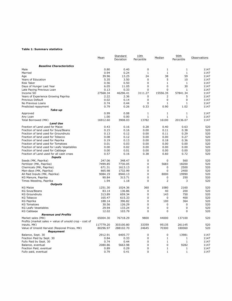
Table 1: Summary statistics

MeanStandard

Deviation

10th

PercentileMedian

90th

PercentileObservations

Baseline Characteristics

Male 0.80 0.40 0 1 1 1147

Married 0.94 0.24 1 1 1 1147

Age 39.96 13.25 24 38 59 1147

Years of Education 5.35 3.50 0 5 10 1147

Risk Taker 0.56 0.50 0 1 1 1147

Days of Hunger Last Year 6.05 11.05 0 0 30 1147

Late Paying Previous Loan 0.13 0.33 0 0 1 1147

Income SD 27568.34 46296.41 3111.27 15556.35 57841.34 1147

Years of Experience Growing Paprika 2.22 2.36 0 2 5 1147

Previous Default 0.02 0.14 0 0 0 1147

No Previous Loans 0.74 0.44 0 1 1 1147

Predicted repayment 0.79 0.26 0.33 0.90 1.02 1147

Take-up

Approved 0.99 0.08 1 1 1 1147

Any Loan 1.00 0.00 1 1 1 1147

Total Borrowed (MK) 16912.60 3908.03 13782 16100 20136.07 1147

Land Use

Fraction of Land used for Maize 0.43 0.16 0.28 0.40 0.63 520

Fraction of land used for Soya/Beans 0.15 0.16 0.00 0.11 0.38 520

Fraction of land used for Groundnuts 0.13 0.12 0.00 0.11 0.29 520

Fraction of land used for Tobacco 0.08 0.12 0.00 0.00 0.27 520

Fraction of land used for Paprika 0.19 0.13 0.00 0.18 0.36 520

Fraction of land used for Tomatoes 0.01 0.03 0.00 0.00 0.00 520

Fraction of land used for Leafy Vegetables 0.00 0.02 0.00 0.00 0.00 520

Fraction of land used for Cabbage 0.00 0.01 0.00 0.00 0.00 520

Fraction of Land used for all cash crops 0.57 0.16 0.38 0.60 0.72 520

Inputs

Seeds (MK, Paprika) 247.06 348.47 0 0 560 520

Fertilizer (MK, Paprika) 7499.85 7730.05 0 5683 18200 520

Chemicals (MK, Paprika) 671.31 1613.13 0 0 2500 520

Man-days (MK, Paprika) 665.98 1732.99 0 0 2400 520

All Paid Inputs (MK, Paprika) 9084.19 8940.13 0 8000 19990 520

KG Manure, Paprika 90.84 313.71 0 0 250 520

Times Weeding, Paprika 1.94 1.18 0 2 3 520

Outputs

KG Maize 1251.30 1024.36 360 1080 2160 520

KG Soya/Beans 83.14 136.86 0 40 200 520

KG Groundnuts 313.89 659.34 0 143 750 520

KG Tobacco 165.47 615.33 0 0 400 520

KG Paprika 188.14 396.82 0 100 364 520

KG Tomatoes 30.56 126.29 0 0 0 520

KG Leafy Vegetables 29.94 133.24 0 0 0 520

KG Cabbage 12.02 103.79 0 0 0 520

Revenue and Profits

Market sales (MK) 65004.30 76718.29 9800 44000 137100 520

Profits (market sales + value of unsold crop - cost of

inputs, MK) 117779.20 303100.80 33359 95135 261145 520

Value of Unsold Harvest (Regional Prices, MK) 80296.97 288102.70 24645 70300 180060 520

Repayment

Balance, Sept. 30 2912.91 6405.77 0 0 13981 1147

Fraction Paid by Sept. 30 0.84 0.33 0 1 1 1147

Fully Paid by Sept. 30 0.74 0.44 0 1 1 1147

Balance, eventual 2080.86 5663.98 0 0 9282 1147

Fraction Paid, eventual 0.89 0.29 0 1 1 1147

Fully paid, eventual 0.79 0.41 0 1 1 1147

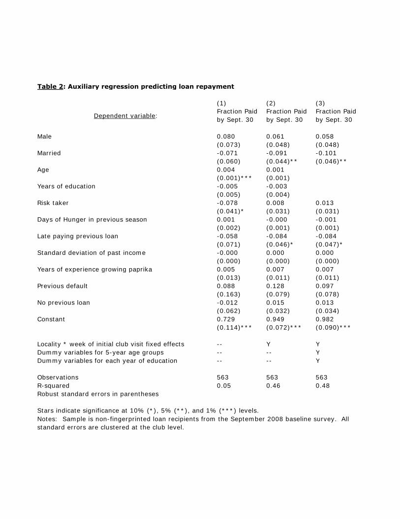
(1) (2) (3)

Dependent variable:Fraction Paid by Sept. 30

Fraction Paid by Sept. 30

Fraction Paid by Sept. 30

Male 0.080 0.061 0.058(0.073) (0.048) (0.048)

Married -0.071 -0.091 -0.101(0.060) (0.044)** (0.046)**

Age 0.004 0.001(0.001)*** (0.001)

Years of education -0.005 -0.003(0.005) (0.004)

Risk taker -0.078 0.008 0.013(0.041)* (0.031) (0.031)

Days of Hunger in previous season 0.001 -0.000 -0.001(0.002) (0.001) (0.001)

Late paying previous loan -0.058 -0.084 -0.084(0.071) (0.046)* (0.047)*

Standard deviation of past income -0.000 0.000 0.000(0.000) (0.000) (0.000)

Years of experience growing paprika 0.005 0.007 0.007(0.013) (0.011) (0.011)

Previous default 0.088 0.128 0.097(0.163) (0.079) (0.078)

No previous loan -0.012 0.015 0.013(0.062) (0.032) (0.034)

Constant 0.729 0.949 0.982(0.114)*** (0.072)*** (0.090)***

Locality * week of initial club visit fixed effects -- Y YDummy variables for 5-year age groups -- -- YDummy variables for each year of education -- -- Y

Observations 563 563 563R-squared 0.05 0.46 0.48

Table 2: Auxiliary regression predicting loan repayment

Stars indicate significance at 10% (*), 5% (**), and 1% (***) levels.

Robust standard errors in parentheses

Notes: Sample is non-fingerprinted loan recipients from the September 2008 baseline survey. All standard errors are clustered at the club level.

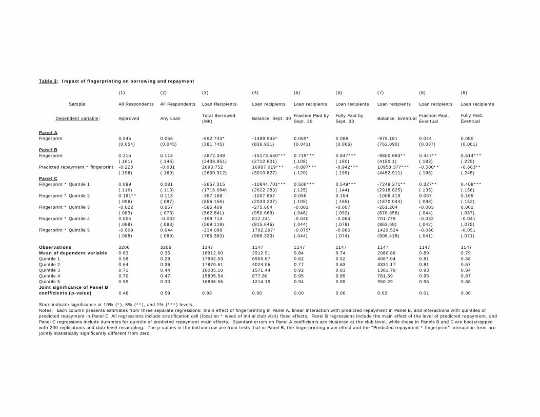
(1) (2) (3) (4) (5) (6) (7) (8) (9)

Sample: All Respondents All Respondents Loan Recipients Loan recipients Loan recipients Loan recipients Loan recipients Loan recipients Loan recipients

Dependent variable: Approved Any Loan Total Borrowed (MK) Balance, Sept. 30 Fraction Paid by

Sept. 30Fully Paid by Sept. 30 Balance, Eventual Fraction Paid,

EventualFully Paid, Eventual

Panel AFingerprint 0.045 0.056 -692.743* -1489.945* 0.069* 0.088 -975.181 0.044 0.080

(0.054) (0.045) (381.745) (836.931) (0.041) (0.066) (762.090) (0.037) (0.061)Panel BFingerprint 0.215 0.118 -2872.348 -15173.560*** 0.719*** 0.847*** -9800.693** 0.447** 0.614***

(.161) (.146) (2438.851) (2712.601) (.108) (.180) (4150.1) (.183) (.225)Predicted repayment * fingerprint -0.220 -0.081 2693.752 16987.019*** -0.807*** -0.942*** 10958.377*** -0.500** -0.663**

(.196) (.169) (2630.912) (3010.827) (.120) (.199) (4452.911) (.196) (.245)Panel CFingerprint * Quintile 1 0.099 0.081 -2657.315 -10844.701*** 0.506*** 0.549*** -7249.271** 0.327** 0.408***

(.116) (.113) (1716.684) (2622.283) (.125) (.144) (2918.825) (.135) (.156)Fingerprint * Quintile 2 0.191** 0.113 -357.168 -1007.857 0.056 0.154 -1006.419 0.057 0.165 (.096) (.087) (856.156) (2033.207) (.105) (.165) (1870.044) (.098) (.152)Fingerprint * Quintile 3 -0.022 0.057 -585.469 -275.604 -0.001 -0.007 -261.204 -0.003 0.002

(.083) (.073) (562.841) (950.669) (.048) (.092) (878.856) (.044) (.087)Fingerprint * Quintile 4 0.004 -0.032 -198.714 812.241 -0.040 -0.064 701.779 -0.032 -0.041

(.088) (.083) (569.119) (915.645) (.044) (.078) (863.69) (.042) (.075)Fingerprint * Quintile 5 -0.009 0.044 -234.098 1702.297* -0.075* -0.085 1429.524 -0.060 -0.051 (.088) (.089) (765.383) (968.333) (.044) (.074) (906.418) (.041) (.071)

Observations 3206 3206 1147 1147 1147 1147 1147 1147 1147Mean of dependent variable 0.63 0.35 16912.60 2912.91 0.84 0.74 2080.86 0.89 0.79Quintile 1 0.58 0.29 17992.53 6955.67 0.62 0.52 4087.04 0.81 0.68Quintile 2 0.64 0.36 17870.61 4024.05 0.77 0.63 3331.17 0.81 0.67Quintile 3 0.71 0.44 16035.10 1571.44 0.92 0.83 1301.79 0.93 0.84Quintile 4 0.70 0.47 15805.54 877.80 0.95 0.85 781.59 0.95 0.87Quintile 5 0.59 0.30 16886.56 1214.19 0.94 0.85 950.29 0.95 0.88Joint significance of Panel B coefficients (p-value) 0.48 0.59 0.88 0.00 0.00 0.00 0.02 0.01 0.00

Notes: Each column presents estimates from three separate regressions: main effect of fingerprinting in Panel A, linear interaction with predicted repayment in Panel B, and interactions with quintiles of predicted repayment in Panel C. All regressions include stratification cell (location * week of initial club visit) fixed effects. Panel B regressions include the main effect of the level of predicted repayment, and Panel C regressions include dummies for quintile of predicted repayment main effects. Standard errors on Panel A coefficients are clustered at the club level, while those in Panels B and C are bootstrapped with 200 replications and club-level resampling. The p-values in the bottom row are from tests that in Panel B, the fingerprinting main effect and the "Predicted repayment * fingerprint" interaction term are jointly statistically significantly different from zero.

Table 3: Impact of fingerprinting on borrowing and repayment

Stars indicate significance at 10% (*), 5% (**), and 1% (***) levels.

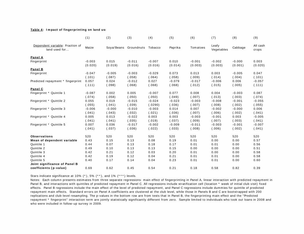
(1) (2) (3) (4) (5) (6) (7) (8) (9)

Dependent variable: Fraction of land used for… Maize Soya/Beans Groundnuts Tobacco Paprika Tomatoes Leafy

Vegetables Cabbage All cash crops

Panel AFingerprint -0.003 0.015 -0.011 -0.007 0.010 -0.001 -0.002 -0.000 0.003

(0.020) (0.019) (0.016) (0.016) (0.014) (0.003) (0.003) (0.001) (0.020)Panel BFingerprint -0.047 -0.005 -0.003 -0.029 0.073 0.013 0.003 -0.005 0.047

(.101) (.087) (.058) (.064) (.058) (.009) (.014) (.004) (.101)Predicted repayment * fingerprint 0.057 0.024 -0.012 0.027 -0.079 -0.017 -0.006 0.006 -0.057

(.111) (.098) (.068) (.068) (.068) (.012) (.015) (.005) (.111)Panel CFingerprint * Quintile 1 -0.087 0.002 0.005 -0.007 0.077 0.008 0.004 -0.003 0.087

(.074) (.058) (.050) (.050) (.049) (.007) (.013) (.003) (.074)Fingerprint * Quintile 2 0.055 0.019 -0.015 -0.024 -0.023 -0.003 -0.008 -0.001 -0.055 (.055) (.041) (.039) (.0290) (.036) (.007) (.008) (.002) (.055)Fingerprint * Quintile 3 -0.006 -0.000 -0.010 -0.003 0.014 0.007 -0.002 -0.000 0.006

(.041) (.043) (.032) (.021) (.036) (.007) (.006) (.002) (.041)Fingerprint * Quintile 4 0.005 0.013 -0.022 0.003 0.003 -0.003 -0.001 0.003 -0.005

(.041) (.041) (.035) (.019) (.037) (.009) (.007) (.003) (.041)Fingerprint * Quintile 5 0.007 0.036 -0.017 -0.002 -0.009 -0.011 -0.003 -0.001 -0.007 (.041) (.037) (.036) (.022) (.033) (.008) (.006) (.002) (.041)

Observations 520 520 520 520 520 520 520 520 520Mean of dependent variable 0.43 0.15 0.13 0.08 0.19 0.01 0.00 0.00 0.57Quintile 1 0.44 0.07 0.13 0.18 0.17 0.01 0.01 0.00 0.56Quintile 2 0.49 0.10 0.13 0.13 0.15 0.00 0.00 0.00 0.51Quintile 3 0.42 0.21 0.12 0.03 0.20 0.01 0.00 0.00 0.58Quintile 4 0.42 0.19 0.12 0.04 0.21 0.01 0.01 0.00 0.58Quintile 5 0.40 0.17 0.14 0.04 0.23 0.01 0.01 0.00 0.60Joint significance of Panel B coefficients (p-value) 0.69 0.62 0.45 0.54 0.21 0.18 0.58 0.82 0.39

Notes: Each column presents estimates from three separate regressions: main effect of fingerprinting in Panel A, linear interaction with predicted repayment in Panel B, and interactions with quintiles of predicted repayment in Panel C. All regressions include stratification cell (location * week of initial club visit) fixed effects. Panel B regressions include the main effect of the level of predicted repayment, and Panel C regressions include dummies for quintile of predicted repayment main effects. Standard errors on Panel A coefficients are clustered at the club level, while those in Panels B and C are bootstrapped with 200 replications and club-level resampling. The p-values in the bottom row are from tests that in Panel B, the fingerprinting main effect and the "Predicted repayment * fingerprint" interaction term are jointly statistically significantly different from zero. Sample limited to individuals who took out loans in 2008 and who were included in follow-up survey in 2009.

Stars indicate significance at 10% (*), 5% (**), and 1% (***) levels.

Table 4: Impact of fingerprinting on land use

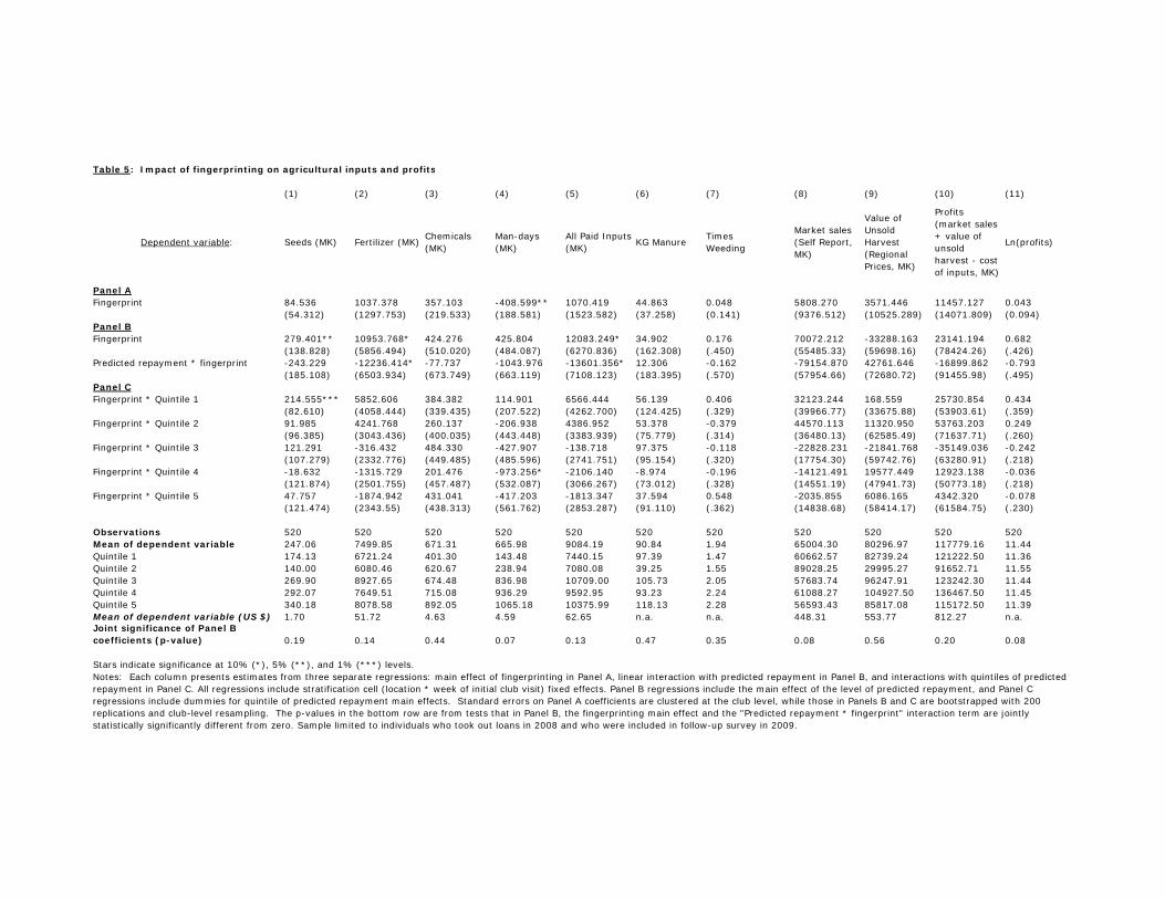
(1) (2) (3) (4) (5) (6) (7) (8) (9) (10) (11)

Dependent variable: Seeds (MK) Fertilizer (MK) Chemicals (MK)

Man-days (MK)

All Paid Inputs (MK) KG Manure Times

Weeding

Market sales (Self Report, MK)

Value of Unsold Harvest (Regional Prices, MK)

Profits (market sales + value of unsold harvest - cost of inputs, MK)

Ln(profits)

Panel AFingerprint 84.536 1037.378 357.103 -408.599** 1070.419 44.863 0.048 5808.270 3571.446 11457.127 0.043

(54.312) (1297.753) (219.533) (188.581) (1523.582) (37.258) (0.141) (9376.512) (10525.289) (14071.809) (0.094)Panel BFingerprint 279.401** 10953.768* 424.276 425.804 12083.249* 34.902 0.176 70072.212 -33288.163 23141.194 0.682

(138.828) (5856.494) (510.020) (484.087) (6270.836) (162.308) (.450) (55485.33) (59698.16) (78424.26) (.426)Predicted repayment * fingerprint -243.229 -12236.414* -77.737 -1043.976 -13601.356* 12.306 -0.162 -79154.870 42761.646 -16899.862 -0.793

(185.108) (6503.934) (673.749) (663.119) (7108.123) (183.395) (.570) (57954.66) (72680.72) (91455.98) (.495)Panel CFingerprint * Quintile 1 214.555*** 5852.606 384.382 114.901 6566.444 56.139 0.406 32123.244 168.559 25730.854 0.434

(82.610) (4058.444) (339.435) (207.522) (4262.700) (124.425) (.329) (39966.77) (33675.88) (53903.61) (.359)Fingerprint * Quintile 2 91.985 4241.768 260.137 -206.938 4386.952 53.378 -0.379 44570.113 11320.950 53763.203 0.249 (96.385) (3043.436) (400.035) (443.448) (3383.939) (75.779) (.314) (36480.13) (62585.49) (71637.71) (.260)Fingerprint * Quintile 3 121.291 -316.432 484.330 -427.907 -138.718 97.375 -0.118 -22828.231 -21841.768 -35149.036 -0.242

(107.279) (2332.776) (449.485) (485.596) (2741.751) (95.154) (.320) (17754.30) (59742.76) (63280.91) (.218)Fingerprint * Quintile 4 -18.632 -1315.729 201.476 -973.256* -2106.140 -8.974 -0.196 -14121.491 19577.449 12923.138 -0.036

(121.874) (2501.755) (457.487) (532.087) (3066.267) (73.012) (.328) (14551.19) (47941.73) (50773.18) (.218)Fingerprint * Quintile 5 47.757 -1874.942 431.041 -417.203 -1813.347 37.594 0.548 -2035.855 6086.165 4342.320 -0.078 (121.474) (2343.55) (438.313) (561.762) (2853.287) (91.110) (.362) (14838.68) (58414.17) (61584.75) (.230)

Observations 520 520 520 520 520 520 520 520 520 520 520Mean of dependent variable 247.06 7499.85 671.31 665.98 9084.19 90.84 1.94 65004.30 80296.97 117779.16 11.44Quintile 1 174.13 6721.24 401.30 143.48 7440.15 97.39 1.47 60662.57 82739.24 121222.50 11.36Quintile 2 140.00 6080.46 620.67 238.94 7080.08 39.25 1.55 89028.25 29995.27 91652.71 11.55Quintile 3 269.90 8927.65 674.48 836.98 10709.00 105.73 2.05 57683.74 96247.91 123242.30 11.44Quintile 4 292.07 7649.51 715.08 936.29 9592.95 93.23 2.24 61088.27 104927.50 136467.50 11.45Quintile 5 340.18 8078.58 892.05 1065.18 10375.99 118.13 2.28 56593.43 85817.08 115172.50 11.39Mean of dependent variable (US $) 1.70 51.72 4.63 4.59 62.65 n.a. n.a. 448.31 553.77 812.27 n.a.Joint significance of Panel B coefficients (p-value) 0.19 0.14 0.44 0.07 0.13 0.47 0.35 0.08 0.56 0.20 0.08

Notes: Each column presents estimates from three separate regressions: main effect of fingerprinting in Panel A, linear interaction with predicted repayment in Panel B, and interactions with quintiles of predicted repayment in Panel C. All regressions include stratification cell (location * week of initial club visit) fixed effects. Panel B regressions include the main effect of the level of predicted repayment, and Panel C regressions include dummies for quintile of predicted repayment main effects. Standard errors on Panel A coefficients are clustered at the club level, while those in Panels B and C are bootstrapped with 200 replications and club-level resampling. The p-values in the bottom row are from tests that in Panel B, the fingerprinting main effect and the "Predicted repayment * fingerprint" interaction term are jointly statistically significantly different from zero. Sample limited to individuals who took out loans in 2008 and who were included in follow-up survey in 2009.

Table 5: Impact of fingerprinting on agricultural inputs and profits

Stars indicate significance at 10% (*), 5% (**), and 1% (***) levels.

Online appendix page 1

NOT FOR PUBLICATION Online Appendix (to be posted on the web upon publication) for Credit Market Consequences of Improved Personal Identification: Field Experimental Evidence from Malawi Appendix A: Background on project partners, loan details, and full text of training script

Background on Cheetah Paprika (CP) Extension services provided by CP consist of preliminary meetings to market paprika

seed to farmers and teach them about the growing process, additional group trainings about farming techniques, individual support for growers provided by the field assistants, and information about grading and marketing the crop. The farmer receives extension services and a package of seeds, pesticides and fungicides at wholesale rates in exchange for the commitment to sell the paprika crop to CP at harvest time. Although CP is by far the largest paprika purchaser in the country, it does not provide credit to farmers because of the risks involved in contract enforcement.1 CP has a staff of six extension officers and 15 field assistants in the locations chosen for the study. The staff maintain a database of all current and past paprika growers and handles the logistics of supplying farmers with the package of inputs as well as the purchase of the crop.

In July 2007, CP asked farmers in the study areas to organize themselves into clubs of 15 to 20 members to accommodate MRFC’s group lending rules.2 Most of these clubs were already in existence, primarily to ease delivery of Cheetah extension services and collection of the crop. During the baseline survey and fingerprinting period (August and September 2007), CP staff provided a list of paprika growing clubs in each locality to be visited in each week.

Background on MRFC and loan details MRFC is a government-owned microfinance institution and is the largest provider of

rural finance, with a nationwide outreach of 210,000 borrowers in 2007. To obtain the loan-financed production inputs, borrowers took an authorization form from MRFC to a pre-approved agricultural input supplier who provided the inputs to the farmer and billed MRFC at a later date. Sixty percent of the loan went towards fertilizer (one 50 kilogram bag of D-compound fertilizer and two 50 kilogram bags of CAN fertilizer); the rest went toward the CP input package: thirty-three percent covered the cost of nine bags of pesticides and fungicides (2 Funguran, 2 Dithane, 2 Benomyl, 1 Cypermethrin, 1 Acephate and 1 Malathion) and the remaining seven percent for

1 In 2007, CP purchased approximately eighty-five percent of the one thousand tons of paprika produced annually in Malawi. 2 A typical CP group has between 15 and 30 farmers and is organized around a paprika collection point. MRFC’s lending groups have at most 20 farmers, so some of the CP groups participating in the study had to be split to be able to access MRFC’s loans.

Online appendix page 2

the purchase of 0.4 kilograms of seeds.3 While all farmers that took the loan were given the CP package, farmers had the option to borrow only one of the two available bags of CAN fertilizer. Expected yield for farmers using the package with two bags of CAN fertilizer on one acre of land was between 400 and 600 kg, compared to 200 kg with no inputs.4 In keeping with standard MRFC practices, farmers were expected to raise a 15 percent deposit, and were charged interest of 33 percent per year (or 30 percent for repeat borrowers). Biometric training script Benefits of Good Credit Having a record of paying back your loans can help you get bigger loans or better interest rates. Credit history works like trust. When you know someone for a long time, and that person is honest and fair when you deal with him, then you trust him. You are more likely to help him, and he is more likely to help you. You might let him use your hoe (or something else that is important to you), because you feel sure that he will give it back to you. Banks feel the same way about customers who have been honest and careful about paying back their loans. They trust those customers, and are more willing to let them borrow money. MRFC already gives customers who have been good borrowers a reward. It charges them a lower interest rate, 30 percent instead of 33 percent. That means that for the loan we have described today, someone who has a good credit history would only have to pay back 8855, instead of 8971.5 Another way that banks might reward customers they trust is by letting them borrow bigger amounts of money. Instead of 7700 MK to grow one acre of paprika, MRFC might lend a trusted customer 15400, to grow two acres. To earn trust with the bank, and get those rewards, you have to be able to prove to the bank that you have taken loans before and paid them back on time. You can do that by making sure that you give the bank accurate information when you fill out loan applications. But if you call yourself John Jacob Phiri one year, and Jacob John Phiri the next year, then the bank might not figure out that you are the same person, so they won’t give you the rewards you have earned. Costs of Bad Credit But trust can be broken. If your neighbor borrows your radio and does not give it back or it gets ruined, then you probably wouldn’t lend him anything else until the radio had been replaced. Banks work the same way. If you take a loan and break the trust between yourself and the bank by not paying back the loan, then the bank won’t lend to you again. This is especially true if you have a good harvest but still choose not to pay back the loan. When you apply for a loan, one of the things that a bank does to decide whether or not to accept your application is to look in its records to see if you have borrowed money before. If you have borrowed but not paid back, then you will be turned down for the new loan. This is like you asking your neighbors if someone new shows up in the village and asks you to work for him. You might first ask around to see if the person is fair to his employees and

3 The loan amount varied across locations because of modest differences in the transport cost for fertilizer. The cost of the CP package was the same in all locations. 4 Yield is computed under the conservative assumption that farmers will divert one 50 Kg bag of CAN fertilizer towards maize cultivation. While larger quantities of inputs would result in higher output for experienced paprika-growers, the package described here was designed by extension experts to maximize expected profits for novice, small-holder growers. 5 Loan amounts mentioned in the script are lower than actual loan amounts observed in the data because fertilizer prices rose somewhat in the time between the initial intervention (in Aug-Sep 2007) and loan disbursement (Nov 2007).

Online appendix page 3

pays them on time. If you learn that the person does not pay his workers, then you won’t work for him. Banks do the same thing by checking their records. MRFC does not ever give new loans to people who still owe them money. And MRFC shares information about who owes money with other banks, so if you fail to pay back a loan from MRFC, it can stop you from getting a new loan from OIBM or another lender, also. Remainder of script is administered to fingerprinted clubs only Biometric Technology Fingerprints are unique, which means that no two people can ever have the same fingerprints. Even if they look similar on a piece of paper, people with special training, or special computer equipment, can always tell them apart. Your fingerprint can never change. It will be the same next year as it is this year. Just like the spots on a goat are the same as long as the goat lives, but different goats have different spots. Fingerprints can be collected with ink and paper, or they can be collected with special machines. This machine stores fingerprints in a computer. Once your fingerprint is stored in the computer, then the machine can recognize you, and know your name and which village you come from, just by your fingerprint! The machine will recognize you even if the person who is using it is someone you have never met before. The information from the machines is saved in many different ways, so if one machine breaks, the information is still there. Just like when Celtel’s building burned, people’s phone numbers did not change. Administer the following after all fingerprints have been collected: Demo Now, I can figure out your name even if you don’t tell me. Will someone volunteer to test me? (Have a volunteer swipe his finger, and then tell everyone who it was). The bank will store information about your loans with your fingerprint. That means that bank officers will know not just your name, but also what loans you have taken and whether or not you have paid them back. They will be able to tell all of this just by having you put your finger on the machine. Before, banks used your name and other information to find out about your credit history. But now they will use fingerprints to find out. This means that even if you tell the bank a different name, they will still be able to find all of your loan records. Names can change, but fingerprints cannot. Having your fingerprint on file can make it easier to earn the rewards for good credit history that we talked about earlier. It will be easy for the bank to look up your records and see that you have paid back your loans before. It will also be easier to apply for loans, because there will be no new forms to fill out in the future! But, having your fingerprint on file also makes the punishment for not paying back your loan much more certain. Even if you tell the bank a different name than you used before, or meet a different loan officer, or go to a different branch, the bank will just have to check your fingerprint to find out whether or not you paid your loans before. Having records of fingerprints also makes it easy for banks to share information. Banks will share information about your fingerprints and loans. If you don’t pay back a loan to MRFC, OIBM will know about it! Appendix B: Details on biometric fingerprinting technology

In consultation with MRFC’s management, fingerprint recognition was chosen over face, iris or retina recognition because it is the cheapest, best known and most widely used biometric identification technology. Fingerprinting technology extracts features from impressions made by the distinct ridges on the fingertips and has been commercially available since the early 1970s.

Online appendix page 4

Loan applicants from fingerprinted clubs had the image of their right thumb fingerprint captured by an optical fingerprint scanner attached to a laptop. To maximize accuracy, farmers washed their thumbprints prior to scanning, and the scanner was also cleaned after each impression. During collection, about 2 per cent of farmers had the left thumbprint recorded (instead of the right) because the right thumbprint was worn out. (Many farmers grow tobacco, which involves thumb usage during seedling transplantation that can wear out a thumbprint over many years.)

Upon scanning, the fingerprint image was enhanced and added to the borrower database. We purchased the VeriFinger 5.0 Software Development Kit from Fulcrum Biometrics and had a programmer develop a data capture program that would allow the user to (i) enter basic demographic information such as the name, address, village, loan size and the unique BFIRM identifier, (ii) capture the fingerprint with the scanner and (iii) review the fingerprint alongside the demographic information. Appendix C: Variable definitions Data used in this paper come from two surveys: a baseline conducted in August-September 2007 and a follow-up survey about farm outputs and other outcomes conducted in August 2008. We also used administrative data about loan take-up and repayment, obtained from MRFC’s internal records. Baseline characteristics (from baseline survey) Male equals 1 for men and 0 for women. Married equals 1 for married respondents and 0 for respondents who are single, widowed, or divorced. Age is respondent’s age in years. In regressions, we use dummies for 5-year age categories rather than a continuous measure of age. Years of education is years of completed schooling, and is top-coded at 13. In regressions, we use dummies for years of completed schooling, rather than a continuous measure of education. Risk taker equals 1 for respondents who report that they frequently take risks, and 0 for respondents who do not. Days of hunger last year is the number of days in the 2006-2007 season that individuals reduced the number of meals they ate per day. Late paying previous loan equals 1 for respondents who report paying back a previous loan late, and 0 for respondents who do not. Income SD is the standard deviation of income between the self-reported best and worst incomes of the 5 most recent years. Years of experience growing paprika is the self reported number of seasons in which the respondent has grown paprika before the season studied in this project. Previous default equals 1 for respondents who report that they have defaulted on a previous loan and 0 otherwise. No previous loans equals 1 for respondents who report that they have not had any other loans from formal financial institutions (including micro lenders, savings and credit cooperatives, and NGO schemes) and 0 otherwise.

Online appendix page 5

Take-up and repayment (from administrative data) Approved equals 1 if the respondent was approved by MRFC for a loan and 0 otherwise. Any loan equals 1 if the respondent borrowed money from MRFC and 0 otherwise (this could differ from Approved if the respondent chose not to take out the loan after it was approved by MRFC). Total borrowed is the amount owed to MRFC, in Malawi kwacha (MK 145 = $US 1). This includes the loan principal and 33 percent interest charged by MRFC. Balance is the unpaid loan amount remaining to be paid to MRFC. The balance includes principal and accumulated interest, and is reported in MK. Fraction paid is the amount paid on the loan, divided by the total borrowed defined above. Fully paid equals 1 if the respondent has completely repaid the loan and 0 if there is an outstanding balance. We examine different versions of the variables Balance, Fraction paid, and Fully paid that vary by the date at which loan repayment status is measured. One set of variables refers to loan repayment status as of September 30, 2008, which is the formal due date of the loan. Another set of variables refers to “eventual” repayment as of the end of November 2008. MRFC considers loan repayment status at the end of November 2008 as the final repayment status of the loan, and makes no subsequent attempts to collect loan repayments after that point. Land use and inputs (from follow-up survey) Fraction of land used for various crops is the land used for the given crop, divided by total land cultivated. Seeds is the value of paprika seeds used by the respondent, in MK. Fertilizer is the value of all chemical fertilizer used by the respondent on the paprika crop, in MK. Chemicals is the value of all pesticides and herbicides used by the respondent on the paprika crop, in MK. Man-days is the amount of money spent on hired, non-family labor for the paprika crop, in MK. All paid inputs is the total amount of money spent on inputs for the paprika crop, in MK. Mathematically, it is the sum of Seeds, Fertilizer, Chemicals, and Man-days defined above. KG manure is the kilograms of manure applied to the paprika crop. Times weeding is the number of times the paprika crop was weeded, by the respondent or hired labor. Output, revenue and profits (from follow-up survey) KG of various crops is the self-reported kilograms harvested of each crop. Market sales is the amount of MK received from any sales of maize, soya, groundnuts, tobacco, paprika, tomatoes, leafy vegetables, and cabbage between April and August, which encompasses the entire main harvest and selling season for these crops.

Online appendix page 6

Profits is the value of Market sales, plus the value of unsold crop estimated based on the farmer’s reported quantity, valued at district average price reported by the EPA office (Value of unsold harvest, defined below), minus All paid inputs as defined above. Value of unsold harvest is the value, in MK, of the difference between the kg harvested and the kg sold of each crop. We use district average prices, as reported by the EPA office. Appendix D: The Model

By virtue of the experiment, the credit contract is kept fixed, so our goal here is not to solve for the optimal contract in the presence of both information asymmetries (Gesnerie, Picard and Rey, 1988 or Chassagnon and Chiappori, 1997 for risk averse agents), but rather to derive the agents’ optimal behavior with and without dynamic incentives.

Agents (or farmers) are risk-neutral and decide how much to borrow for cash crop inputs and how much to invest. We assume that they do not have collateral or liquid assets, so the maximum they can invest in cash crop production is the loan amount.

We introduce the possibility of adverse selection by allowing farmers to differ in the probability p (unobserved by the lender) that cash crop production is successful. Production is

given by )(bfS when successful and by )(bfF when it fails, which happens with

probability p1 . The amount b denotes total cash crop inputs invested. We assume that )(bf j ,

SFj , satisfies the usual properties 0)0( jf , 0)( bf j and 0)( bf j .

We model moral hazard by allowing borrowers to divert inputs instead of investing them in cash crop production. The decision to divert inputs is not observable by the lender. If they decide to divert, they earn q per unit of input diverted, which can be interpreted as the secondary market price for inputs or the expected return if these inputs are invested in another crop. Given the arrangement to buy the cash crop (paprika) in the experiment, we assume that the lender can only seize cash crop production but not the proceeds from diverted inputs. To simplify matters, we assume that the choice of diversion is binary, that is, either all or nothing is diverted.6

Following the experiment, the credit contract offered by the lender is given by a loan amount b and gross interest rate R , regardless of whether the lender can use dynamic incentives. We assume that the loan size b can take on two values, Lb and Hb where HL bb .7 We also assume that even when cash crop production fails, the borrower has enough funds to cover loan repayment provided that the small amount Lb is borrowed and inputs are not diverted. More

formally, Rbbf LLF )( . This assumption and the fact that 0)0( Ff implies that if the borrower

chooses to invest the large amount Hb in paprika production but the crop fails, then the borrower

defaults because by concavity of )(Ff , Rbbf HHF )( . Finally, we assume that if the crop succeeds, the large loan size yields higher farm profits than the smaller loan size. If we

6 One can extend the model to the case where diversion is a continuous variable but the intuition is already captured in the simpler version presented. 7This assumption is in accord with the actual details of the loan package, where the most important determinant of loan size is whether the farmer chooses to have the loan fund one vs. two bags of CAN fertilizer. We can think of

Hb including two bags, and Lb only one.

Online appendix page 7

let Rbbfby kkSkS )()( , for HLk , denote net profits from successful cash crop

production, this assumption can be expressed as )()( LSHS byby .8

We assume that there are two periods and no discounting, although the model could easily be extended to an infinite horizon setting with discounting. The timing within a period follows the set-up of the field experiment: the borrower first learns whether the lender can use dynamic incentives; then the borrower decides how much to borrow and whether to divert inputs; then paprika production takes place; the loan is repaid if sufficient funds are available and finally the borrower consumes any remaining income.

In what follows, we take the credit contract as given and characterize optimal borrower behavior with and without dynamic incentives. Then we briefly discuss the optimality of the credit contract and compare the predictions of the model to those of other models in the literature. Borrower behavior without dynamic incentives

Since the lender is forced to offer the same contract in each period, lifetime optimization coincides with period-by-period optimization. In a given period, the borrower chooses how much to borrow b and whether to divert inputs D by solving the following problem:

)()1(max),()1(maxmax)(

1,01,0,LSL

DHSH

DbbbbpyDDqbbpyDDqbpv

HL

The dependency of net income from borrowing v on p is made explicit. If the borrower diverts, consumption is qb because the bank cannot seize income, but if the borrower invests in paprika production, consumption only takes place when production is successful as the bank seizes all output if paprika production fails.

Now let Dp be the success probability that leaves a borrower with the larger loan size Hb indifferent between diverting the inputs or investing them in paprika production. More formally,

)( HSDH bypqb as plotted in Appendix Figure 2.

If Dpp , the solution to the problem when dynamic incentives are absent is to always

borrow the large amount Hb and to divert all inputs ( 1D ). If Dpp , the borrower also

borrows the large amount Hb but does not divert and therefore repays with probability p. Expected net income in a period )( pv is

Hqbpv )( if Dpp and )()( HS bpypv if Dpp . (1)

Borrower behavior with dynamic incentives In this case, the lender will only provide credit in period two to borrowers that have

successfully repaid in period one. Because there are only two periods, in the last period the lender cannot provide additional incentives to elicit repayment, so the optimization problem that borrowers face is the same as the period-by-period optimization when dynamic incentives were absent. Borrowers maximize their lifetime utility by solving the following problem in period one:

)()()1(max,)()()1(maxmax)(

1,01,0,pvbpyDDqbpvbypDDqbpV LSL

DHSH

Dbbb HL

where again the dependency of V and v on p is made explicit. Net income v in period two is

derived in (1). If the lower amount Lb is chosen, the borrower can always repay the loan and so net income from borrowing )( pv in period two is assured. If, on the other hand, the higher

8 Using similar notation, the previous assumption implies that when the crop fails, farm profits are larger under the

smaller loan size: )()( LFHF byby .

Online appendix page 8

amount Hb is chosen, then the borrower will obtain )( pv in period two only if there is no diversion ( 0D ) and paprika production is successful in period one. Income from not borrowing is normalized to zero.

It is easy to see that with dynamic incentives, diversion of inputs in the first period is never optimal. A borrower with a high probability of success Dpp would not divert in the absence of penalties, so he would certainly not do it when the lender can impose penalties. More formally, because HHS qbbpy )( if Dpp , it follows that HHS qbpvbyp )()( since

0)( pv .

When Dpp , borrowers choose to divert in the absence of dynamic incentives. When dynamic incentives are in place, they can increase lifetime utility by choosing the lower amount in the first period. They then secure a loan in the second period which can then be diverted to achieve the same utility as if they had diverted in the first period. In addition, if cash crop production succeeds, then they also consume in the first period.9

We now study the choice of loan amount in the first period. Let 0Bp be the probability of

success that leaves a borrower with success probability Dpp indifferent between the two loan

amounts. If success probability is such that 0BD ppp , then the borrower chooses Lb to

ensure loan repayment, but if the probability is high enough, so that ppp BD 0 he then

chooses Hb . The subscript 0 denotes the fact that in the absence of dynamic incentives the

borrower would not divert because Dpp . Probability 0Bp can be written as

)(

)(0

HS

LSB by

byp . (2)

Now let 1Bp be analogous to 0Bp for borrowers with success probability Dpp . Here the

subscript 1 indicates that the borrower would divert in the absence of dynamic incentives. If success probability satisfies DB ppp 1 , the borrower will choose the smaller loan amount Lb

and if DB ppp 1 the larger amount Hb . It is easy to show that 1Bp satisfies

)()()1( 11 LSHSBBH bybyppqb (3)

or, after some algebra and substitutions,

01 1 BD

DB pp

pp

. (4)

As it turns out, depending on the magnitude of )( LS by , )( HS by and Hqb only 1BD pp or

0BD pp will hold, because 1BD pp is true if and only if 0BD pp .10 So either 0Bp or 1Bp is

relevant. There are three cases, which we label (i), (ii), and (iii), distinguished by the size of the gains from input diversion ( Hqb ) relative to those from successful cash crop production, )( HS by

and )( LS by .

The first case is where (i) )( HSH byqb , in which the gains from diversion are higher

than the gains from cash crop production even when the high loan amount is taken and

9 While this result is immediate without discounting, it can be obtained with discounting provided the discount rate is low enough. 10 This is easy to see using the expression for 1Bp derived in (4).

Online appendix page 9

production is successful. In this case, 011 BBD ppp and 0Bp becomes irrelevant because

0BD pp is violated. Intuitively, 1Dp means that there are no borrowers who would repay

without dynamic incentives, because the gains from diversion are higher than the gains from cash crop production even for borrowers with the highest success probabilities; 0Bp is irrelevant

because there are no farmers for whom Dpp . In the first period with dynamic incentives,

borrowers with 1Bpp take the larger loan and those for whom 1Bpp take the smaller loan size.

The second – and probably most interesting – case is where (ii) )()( LSHHS byqbby ,

in which the gains from diversion (relative to cash crop production) are intermediate. In this case, in the absence of dynamic incentives, some borrowers (those with highest success probabilities, for whom Dpp ) will choose to produce rather than divert, while others with lower success probabilities will divert rather than produce. In this case we have

011 BBD ppp ,11 and so 0Bp is irrelevant (those with Dpp always choose the larger loan

in the first period). In the first period with dynamic incentives, borrowers with 1Bpp take the

larger loan and those for whom 1Bpp take the smaller loan size.

The third case is where (iii) HLS qbby )( , in which the gains from diversion are small

relative to the gains from successful cash crop production, even when the small loan size is taken. Here, DBB ppp 101 so that 1Bp now becomes irrelevant (because all individuals with

Dpp will take the smaller loan size in the first period with dynamic incentives). Now it is

those borrowers for whom Dpp that show variation in loan size in the first period with

dynamic incentives: those with 0Bpp take the larger loan and those for whom 0Bpp take

the smaller loan size. Appendix Figure 2 is drawn assuming Case (ii) holds. It plots 0Bp and 1Bp , and

because 0BD pp , 0Bp is irrelevant. Probability 1Bp is shown as the intersection of the left hand

side and right hand side of the equality in (3) above. For each regime (with and without dynamic incentives), Appendix Figure 3 reports the

first period optimal choices of loan size and whether to divert as well as repayment rate as a function of the borrowers’ success probability.

Interestingly, and as mentioned in the text, dynamic incentives have different effects on the optimal choices of borrowers depending on their probability of success. For example, borrowers with relatively low probability of success are most affected by the introduction of dynamic incentives. They choose the higher loan amount and to divert it all without dynamic incentives but borrow the lower amount and invest it in cash crop production when dynamic incentives are introduced. As a result, their repayment rate changes from zero to one once incentives are introduced.

Borrowers with relatively high probability of success are the least affected, since they never divert inputs and always choose the higher loan amount, except for in Case (i) where they would divert without incentives and not divert with incentives.

11 To see this, divide inequalities in (ii) by )( HS by and recall )( HSDH bypqb and expression (4).

Online appendix page 10

Borrowers with an intermediate value of the probability of success will, upon introduction of dynamic incentives, change either the diversion or the loan size decisions depending on the parameter values and functional forms. In Case (ii) they always choose the higher loan amount but move from diversion to no diversion when incentives are introduced. In Case (iii), they never divert but incentives lead them to move from the higher to the lower loan amount. Discussion

If the lender sets gross interest rate R to break even, and the individual probability of success ]1,0[p is drawn from the density function )( pG , then R satisfies

)]())|(1()|()][(1[ HFDHDDH bfpppERbpppEpGib , (5)

where i is the deposit rate and 1

)()|(Dp

D ppdGpppE .

Notice that the bank breaks-even whenever 1Dp , otherwise all borrowers would divert and the bank would be unable to collect repayment. As a result, there is no interest rate R such that case (i) considered before is an equilibrium.

Depending on the parameters, a separating equilibrium may exist where the lender maximizes borrower welfare subject to breaking even by offering a menu of loan sizes and gross interest rates. Borrowers with low probability of success p may either borrow the large amount and default or borrow the lower amount and produce (again depending on the parameters), borrowers with intermediate probability of success will borrow the lower amount and produce and borrowers with high probability of success will borrow the large amount and produce.12

When dynamic incentives are introduced, the lender can follow a strategy similar to Stiglitz and Weiss (1983) or Boot and Thakor (1994). In words, the lender could lower the interest rate associated with the lower loan size Lb in the second period below the per period break even interest rate (thereby making a loss) but raise it in the first period so as to satisfy the break even constraint intertemporally. This may be optimal because in the first period the borrower has the added incentive of the promise of a loan in the future, a loan that will be ever more attractive the lower is the interest rate charged.

If collateral was available, then a menu of interest rates and collateral could always be offered in both periods (Bester, 1985). But as Boot and Thakor (1994) point out, dynamic incentives can be more efficient than static incentives like collateral. As in their model, the value of long-term contracting does not arise from the ability to learn the borrower type (in their model all agents are equal) nor from improved risk-sharing (in both models agents are risk neutral). Long term relations are valuable because the lender has the ability to punish defaulters and to reward good borrowers.

Because repayment is higher with dynamic incentives, lenders could lower the interest rate and as a result borrowers might borrow more. The lender should also be willing to extend more credit if dynamic incentives can be used. As a result, overall borrowing could increase, although borrowers with low probability of success may still borrow less to ensure future access to loans. This increase in borrowing is also predicted by the more macro literature that tries to

12 The observation that only a unique (pooling) contract exists may be used to rule out parameter combinations where the separating equilibrium is optimal. Of course, other considerations outside the model may be responsible for only observing one contract, even if it is sub-optimal. For example, before the study MRFC gave only a few loans for paprika and so it may still be learning about the optimal contract.

Online appendix page 11

explain the increase in personal bankruptcies over the last few decades as a result of improvements in information technology available to lenders for credit decisions (see for example Livshits, McGee and Tertilt, forthcoming and 2009; Narajabad, 2010 and Sanchez, 2009).

The source of heterogeneity in the model is the probability of success p . If there was heterogeneity in the discount rate, then dynamic incentives would only be relevant for agents that are patient (ie with low enough discount rate). In this alternative model, if borrowers prefer to divert in the absence of dynamic incentives, repayment would be low without fingerprinting and would only increase for agents with low discount rate when fingerprinting is introduced.

In many multi-period models of limited commitment and asymmetric information, agents are not allowed to save because they could borrow and default and subsequently live in autarky by reinvesting the savings (Bulow and Rogoff, 1989). In Boot and Thakor (1994), the agent has no incentive to save because the long-term contract provides better-than-market interest rates. In this model without dynamic incentives, agents with high probability of success will not find it profitable to default and save for period 2 either, even if a savings technology were available at rate i . But if the probability is low enough, in particular if p is such that

)(

)1(

LS

H

by

qbip

,

then agents would borrow the higher amount Hb in period one, divert and hence default and save it into period 2 to earn 1i . When dynamic incentives are allowed, then the same argument of Boot and Thakor (1994) applies and so agents would prefer to borrow again in the second period, even if savings technology were available. Appendix E: Checking for loan officer responses to fingerprinting

In this appendix section we describe in further detail the findings that loan officers do not appear to have responded to whether or not a club was fingerprinted (summarized in Section 5.A. of the main text). Online Appendix Table 2 examines reports from all loan officers collected in August 2008 as well as borrower responses in the August 2008 follow-up survey. Loan officers were first asked about the specific treatment status of five clubs randomly selected from the sample of clubs for which they were responsible. They were then asked whether they knew the secretary or president of the club and finally they were asked to estimate the number of loans given out in each club. The first row of the table shows that loan officers had very little knowledge about the actual treatment status of clubs. Only 54 percent of the fingerprinted clubs are reported correctly as being fingerprinted and an even lower 22 percent of non-fingerprinted clubs are reported correctly as such. Pure guesswork would yield an accuracy rate of 50 percent. This evidence alone suggests that loan officers did not take into account treatment status in their interactions with the clubs.

Loan officers know club officers roughly half of the time, and on average misreport the number of loans disbursed to a club by 1.5 loans. More importantly, there are no statistical differences in the reporting accuracy of fingerprinted clubs compared to non-fingerprinted ones. Borrower reports in the last three rows of the table paint a similar picture. Loan officers are no more likely to visit non-fingerprinted clubs to collect repayment compared to fingerprinted clubs, and as a result, members of non-fingerprinted clubs report talking the same number of times to

Online appendix page 12

loan officers as do members of fingerprinted clubs. Finally, they all report finding it relatively easy to contact the loan officer.

The evidence in the table indicates that loan officers did not respond to the treatment. Therefore, we interpret impacts of the treatment as emerging solely from borrowers’ responses to being fingerprinted. Appendix F: Additional robustness checks Impact of fingerprinting in full sample

Analyses of the full sample of farmers, without restricting the sample only to borrowers, can help address concerns about selection bias. Appendix Tables 5 and 6 present results from regressions analogous to the main Tables 4 and 5, respectively, with the difference that the regressions include all 1,226 individuals interviewed in the follow-up survey (borrowers plus nonborrowers). Full-sample regression results in Appendix Tables 5 and 6 are very similar to those from the borrower-only regressions. As discussed in the main text, the general pattern is for coefficients that were significant before to remain statistically significant, but to be only around half the magnitude of the coefficients in the borrowing sample regressions. This reduction in coefficient magnitude is consistent with effect sizes in the full sample representing a weighted average of no effects for nonborrowers and nonzero effects for borrowers.

To be specific, in the land-use full-sample regressions (Appendix Table 5), fingerprinting leads farmers in quintile 1 of predicted repayment to devote 5.8 percentage points more of their land to paprika (significant at the 5% level). In the inputs regressions (Appendix Table 6, Columns 1-7), the interaction of fingerprinting with predicted repayment in Panel B is negative and significant at the 5% level in the regressions for fertilizer and all paid inputs, compared to significance at the 10% level in main Table 5. The fingerprinting * (quintile 1) interaction term is also positive and statistically significant at the 10% level or better for all input types in the table except for man-days. Results in the sales and profits regressions of Appendix Table 6, Columns 8-11 are similar to corresponding ones in main Table 5, but as before they are not statistically significantly different from zero. Results with “simple” predicted repayment regression We discuss here robustness of treatment effect heterogeneity results to constructing the predicted repayment variable when excluding the locality*(week of initial club visit) fixed effects. Compared with the predicted repayment regression used in the main results (column 3, Table 2), when (locality)*(week of initial club visit) fixed effects are dropped the R-squared of the regression falls from 0.48 to 0.08. These alternative specifications are reported in Appendix Table 10.

This simpler regression is then used to predict repayment for the full sample, and the predicted repayment variable is interacted with treatment to examine heterogeneity in the treatment effect. Results from this exercise are presented in Appendix Tables 7 through 9, which should be compared (respectively) to the main Tables 3 through 5.

Results are very similar when using this simpler index of predicted repayment. For example, the coefficients on the interaction between linear predicted repayment and fingerprinting in Panel B remain large in magnitude and retain statistical significance in the

Online appendix page 13

repayment and inputs regressions (Appendix Table 7, Columns 4-9, and Appendix Table 9, Columns 1-7, respectively). In Panel C, where fingerprinting is interacted with quintiles of predicted repayment, a slight difference vis-à-vis previous results is that typically the significant interaction term is (fingerprinting)*(quintile 2) rather than the interaction with quintile 1. In sum, the general pattern that fingerprinting has more substantial effects on repayment and activities on the farm for individuals with lower predicted repayment is robust to using this simpler predicted repayment regression. Results where predicted repayment coefficients obtained from partition of control group This section describes our approach to estimating predicted repayment using a partition of the control group separate from a partition used as a counterfactual for the treatment group in the main regressions. We conduct this exercise 1,000 times, where in each replication we first randomly select 50% of the control group for inclusion in the auxiliary regression to predict repayment. We then predict repayment for the other half of the control group and the full treatment group. Finally, we estimate the heterogeneous effects of treatment on repayment, land use, input use, and farm profits using equation (2) on a sample that includes the full treatment group and the half of the control group not randomly chosen for the auxiliary regression.

We report the 95 percent confidence interval for coefficients obtained from this procedure in Appendix Table 11. We focus on results for the interaction between the treatment indicator and the indicator for quintile 1 of predicted repayment.13 Panel A of Appendix Table 11 corresponds to Table 3, Columns 4-9; Panel B corresponds to Table 4; Panel C corresponds to Table 5, Columns 1-7, and Panel D corresponds to Table 5, Columns 8-11. The coefficient and standard error reported are the original estimates and bootstrap replications using the full sample, as described previously.

In every case, the coefficient from the estimate using the full sample falls within the 95 percent confidence interval from the procedure using the partitioned sample. Furthermore, in every case where the original coefficient is significant, all coefficients in the 95 percent confidence interval of the partitioning exercise have the same sign as the coefficient in the main regressions of the paper, and the confidence interval never includes zero. Appendix G: Details of benefit-cost calculation

The benefit-cost calculation is presented in Appendix Table 13. The uppermost section of the table is the calculation of benefits per individual fingerprinted. At the suggestion of MRFC, we assume that all new loan applicants are fingerprinted, and that 50% of applicants are approved for loans. Based on our experimental results we assume that the increase in repayment due to fingerprinting is confined to the first quintile (20% of borrowers), and that for this subgroup fingerprinting causes an increase in repayment amounting to 32.7% of the loan balance (from column 8 of Table 3). We assume that the total amount to be repaid is MK15,000 on average. Total benefit per individual fingerprinted is therefore MK490.50 (US$3.38). The next section of the table calculates cost per individual fingerprinted. There are three general types of costs. First, equipment costs need to be amortized across farmers fingerprinted. We assume each equipment unit (a laptop computer and external fingerprint scanner) costs

13 The confidence interval is the 2.5th to 97.5th percentile of coefficients from the 1,000 replications.

Online appendix page 14

MK101,500,14 and is amortized over three years, for annual cost of each equipment package of MK33,833. Twelve (12) of these equipment packages (two for each of six branches) will be required to fingerprint MRFC’s borrowers throughout the country. With an estimated 5,000 new loan applicants per year, each of these equipment units will be used to fingerprint 417 farmers on average. The equipment cost per farmer fingerprinted is therefore MK81.20. The second type of cost is loan officer time. We estimate that it takes 5 minutes to fingerprint a customer and enter his or her personal information into the database. At a salary of MK40,000 per month and 173.2 work hours per month, this comes out to a cost of MK19.25 per customer fingerprinted. The third type of cost is the transaction cost per fingerprint checked, MK108.75 (US$0.75). We assume here that MRFC hires a private firm to provide the fingerprint identification services, in which case the fingerprint database is stored on the firm’s server overseas and batches of fingerprints to be checked are sent electronically by MRFC to the firm during loan processing season. Lists of identified defaulters are sent back to MRFC with fast turnaround. In consultation with a U.S. private firm that provides such services, we were given a range of $0.03-$0.75 per fingerprint identification transaction. Per-fingerprint transaction costs are higher when the client has a relatively low number of transactions per year, and MRFC’s 5,000 transactions per year is considered low, so we conservatively assume the transaction cost per fingerprint at the higher end of this range, $0.75 (MK108.75). Summing up these three types of costs, total cost per individual fingerprinted is MK209.20. The net benefit per individual fingerprinted is therefore MK281.30 (US$1.94), and the benefit-cost ratio is an attractive 2.34. 15

14 This is the actual cost of each equipment unit we purchased for the project, which included a laptop computer ($480), an extra laptop battery ($120), a laptop carrying case ($20), and an external fingerprint scanner ($80). 15 An alternative is for a lending institution to purchase its own fingerprint matching software and do fingerprint identification in-house instead of subcontracting this function to an outside firm. This would eliminate the $0.75 (MK108.75) transaction cost per fingerprint checked. According to a U.S. fingerprint identification services firm we consulted, the initial fixed cost of installing an off-the-shelf fingerprint matching software system is in the range of $15,000 to $50,000 (depending on specifications), with an annual maintenance cost of 10-20% of the initial fixed cost. In addition, there would be personnel costs for staff to operate the system. Assuming an initial fixed cost of $15,000, maintenance cost of 10% of the original fixed cost, and an additional full-time staff member to run the system costing the same as a current MRFC loan officer, NPV is lower when fingerprint identification is done in-house than when this function is contracted out (which is why Appendix Table 13’s calculation assumes contracting out). But with a high enough annual volume of transactions (perhaps in the context of a credit bureau in which many or all of Malawi’s lenders participate), in-house fingerprint identification could make economic sense.

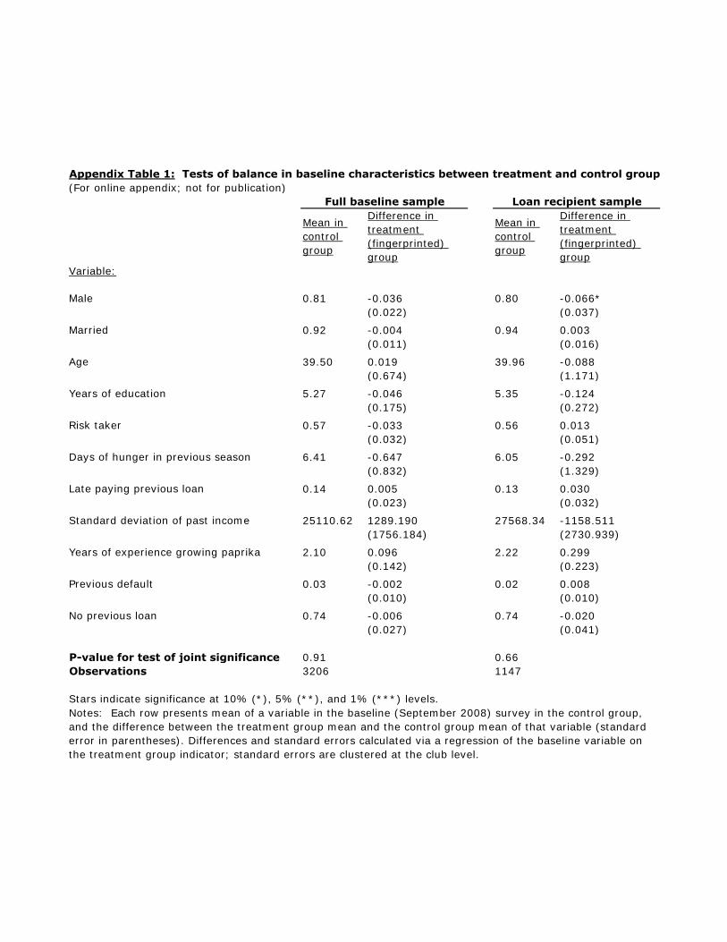
(For online appendix; not for publication)

Mean in control group

Difference in treatment (fingerprinted) group

Mean in control group

Difference in treatment (fingerprinted) group

Variable:

Male 0.81 -0.036 0.80 -0.066*(0.022) (0.037)

Married 0.92 -0.004 0.94 0.003(0.011) (0.016)

Age 39.50 0.019 39.96 -0.088(0.674) (1.171)

Years of education 5.27 -0.046 5.35 -0.124(0.175) (0.272)

Risk taker 0.57 -0.033 0.56 0.013(0.032) (0.051)

Days of hunger in previous season 6.41 -0.647 6.05 -0.292(0.832) (1.329)

Late paying previous loan 0.14 0.005 0.13 0.030(0.023) (0.032)

Standard deviation of past income 25110.62 1289.190 27568.34 -1158.511(1756.184) (2730.939)

Years of experience growing paprika 2.10 0.096 2.22 0.299(0.142) (0.223)

Previous default 0.03 -0.002 0.02 0.008(0.010) (0.010)

No previous loan 0.74 -0.006 0.74 -0.020(0.027) (0.041)

P-value for test of joint significance 0.91 0.66Observations 3206 1147

Loan recipient sampleFull baseline sample

Notes: Each row presents mean of a variable in the baseline (September 2008) survey in the control group, and the difference between the treatment group mean and the control group mean of that variable (standard error in parentheses). Differences and standard errors calculated via a regression of the baseline variable on the treatment group indicator; standard errors are clustered at the club level.

Appendix Table 1: Tests of balance in baseline characteristics between treatment and control group

Stars indicate significance at 10% (*), 5% (**), and 1% (***) levels.

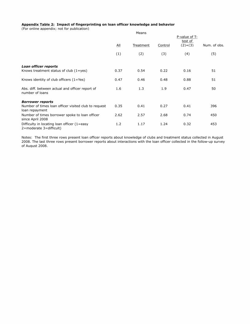
(For online appendix; not for publication)

All Treatment Control

(1) (2) (3) (4) (5)

Loan officer reports

Knows treatment status of club (1=yes) 0.37 0.54 0.22 0.16 51

Knows identity of club officers (1=Yes) 0.47 0.46 0.48 0.88 51

Abs. diff. between actual and officer report of

number of loans

1.6 1.3 1.9 0.47 50

Borrower reports

Number of times loan officer visited club to request

loan repayment

0.35 0.41 0.27 0.41 396

Number of times borrower spoke to loan officer

since April 2008

2.62 2.57 2.68 0.74 450

Difficulty in locating loan officer (1=easy

2=moderate 3=difficult)

1.2 1.17 1.24 0.32 453

Means

P-value of T-

test of

(2)=(3) Num. of obs.

Notes: The first three rows present loan officer reports about knowledge of clubs and treatment status collected in August

2008. The last three rows present borrower reports about interactions with the loan officer collected in the follow-up survey

of August 2008.

Appendix Table 2: Impact of fingerprinting on loan officer knowledge and behavior

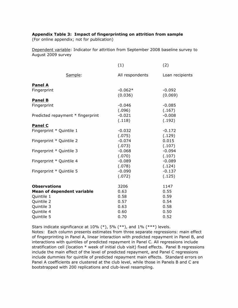
(For online appendix; not for publication)

(1) (2)

Sample: All respondents Loan recipients

Panel A

Fingerprint -0.062* -0.092

(0.036) (0.069)

Panel B

Fingerprint -0.046 -0.085

(.096) (.167)

Predicted repayment * fingerprint -0.021 -0.008

(.118) (.192)

Panel C

Fingerprint * Quintile 1 -0.032 -0.172

(.075) (.129)

Fingerprint * Quintile 2 -0.074 0.015

(.073) (.107)

Fingerprint * Quintile 3 -0.068 -0.094

(.070) (.107)

Fingerprint * Quintile 4 -0.089 -0.089

(.078) (.124)

Fingerprint * Quintile 5 -0.090 -0.137

(.072) (.125)

Observations 3206 1147

Mean of dependent variable 0.63 0.55

Quintile 1 0.58 0.59

Quintile 2 0.57 0.54

Quintile 3 0.63 0.58

Quintile 4 0.60 0.50

Quintile 5 0.70 0.52

Notes: Each column presents estimates from three separate regressions: main effect

of fingerprinting in Panel A, linear interaction with predicted repayment in Panel B, and

interactions with quintiles of predicted repayment in Panel C. All regressions include

stratification cell (location * week of initial club visit) fixed effects. Panel B regressions

include the main effect of the level of predicted repayment, and Panel C regressions

include dummies for quintile of predicted repayment main effects. Standard errors on

Panel A coefficients are clustered at the club level, while those in Panels B and C are

bootstrapped with 200 replications and club-level resampling.

Dependent variable: Indicator for attrition from September 2008 baseline survey to

August 2009 survey

Appendix Table 3: Impact of fingerprinting on attrition from sample

Stars indicate significance at 10% (*), 5% (**), and 1% (***) levels.

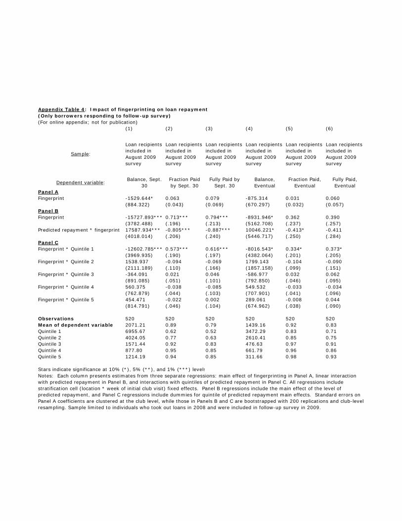
Appendix Table 4: Impact of fingerprinting on loan repayment (Only borrowers responding to follow-up survey)

(1) (2) (3) (4) (5) (6)

Sample:

Loan recipients included in August 2009 survey

Loan recipients included in August 2009 survey

Loan recipients included in August 2009 survey

Loan recipients included in August 2009 survey

Loan recipients included in August 2009 survey

Loan recipients included in August 2009 survey

Dependent variable: Balance, Sept. 30

Fraction Paid by Sept. 30

Fully Paid by Sept. 30

Balance, Eventual

Fraction Paid, Eventual

Fully Paid, Eventual

Panel AFingerprint -1529.644* 0.063 0.079 -875.314 0.031 0.060

(884.322) (0.043) (0.069) (670.297) (0.032) (0.057)Panel BFingerprint -15727.893*** 0.713*** 0.794*** -8931.946* 0.362 0.390

(3782.488) (.196) (.213) (5162.708) (.237) (.257)Predicted repayment * fingerprint 17587.934*** -0.805*** -0.887*** 10046.221* -0.413* -0.411

(4018.014) (.206) (.240) (5446.717) (.250) (.284)Panel CFingerprint * Quintile 1 -12602.785*** 0.573*** 0.616*** -8016.543* 0.334* 0.373*

(3969.935) (.190) (.197) (4382.064) (.201) (.205)Fingerprint * Quintile 2 1538.937 -0.094 -0.069 1799.143 -0.104 -0.090 (2111.189) (.110) (.166) (1857.158) (.099) (.151)Fingerprint * Quintile 3 -364.091 0.021 0.046 -586.977 0.032 0.062

(891.085) (.051) (.101) (792.850) (.046) (.095)Fingerprint * Quintile 4 560.375 -0.038 -0.085 549.532 -0.033 -0.034

(762.879) (.044) (.103) (707.901) (.041) (.096)Fingerprint * Quintile 5 454.471 -0.022 0.002 289.061 -0.008 0.044 (814.791) (.046) (.104) (674.962) (.038) (.090)

Observations 520 520 520 520 520 520Mean of dependent variable 2071.21 0.89 0.79 1439.16 0.92 0.83Quintile 1 6955.67 0.62 0.52 3472.29 0.83 0.71Quintile 2 4024.05 0.77 0.63 2610.41 0.85 0.75Quintile 3 1571.44 0.92 0.83 476.63 0.97 0.91Quintile 4 877.80 0.95 0.85 661.79 0.96 0.86Quintile 5 1214.19 0.94 0.85 311.66 0.98 0.93

(For online appendix; not for publication)

Stars indicate significance at 10% (*), 5% (**), and 1% (***) levelsNotes: Each column presents estimates from three separate regressions: main effect of fingerprinting in Panel A, linear interaction with predicted repayment in Panel B, and interactions with quintiles of predicted repayment in Panel C. All regressions include stratification cell (location * week of initial club visit) fixed effects. Panel B regressions include the main effect of the level of predicted repayment, and Panel C regressions include dummies for quintile of predicted repayment main effects. Standard errors on Panel A coefficients are clustered at the club level, while those in Panels B and C are bootstrapped with 200 replications and club-level resampling. Sample limited to individuals who took out loans in 2008 and were included in follow-up survey in 2009.

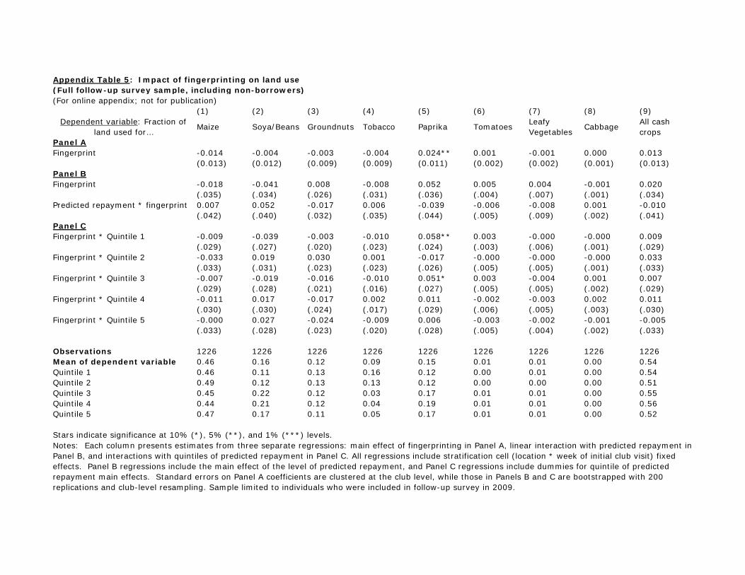
(Full follow-up survey sample, including non-borrowers)

(1) (2) (3) (4) (5) (6) (7) (8) (9)Dependent variable: Fraction of

land used for… Maize Soya/Beans Groundnuts Tobacco Paprika Tomatoes Leafy Vegetables Cabbage All cash

cropsPanel AFingerprint -0.014 -0.004 -0.003 -0.004 0.024** 0.001 -0.001 0.000 0.013

(0.013) (0.012) (0.009) (0.009) (0.011) (0.002) (0.002) (0.001) (0.013)Panel BFingerprint -0.018 -0.041 0.008 -0.008 0.052 0.005 0.004 -0.001 0.020

(.035) (.034) (.026) (.031) (.036) (.004) (.007) (.001) (.034)Predicted repayment * fingerprint 0.007 0.052 -0.017 0.006 -0.039 -0.006 -0.008 0.001 -0.010

(.042) (.040) (.032) (.035) (.044) (.005) (.009) (.002) (.041)Panel CFingerprint * Quintile 1 -0.009 -0.039 -0.003 -0.010 0.058** 0.003 -0.000 -0.000 0.009

(.029) (.027) (.020) (.023) (.024) (.003) (.006) (.001) (.029)Fingerprint * Quintile 2 -0.033 0.019 0.030 0.001 -0.017 -0.000 -0.000 -0.000 0.033 (.033) (.031) (.023) (.023) (.026) (.005) (.005) (.001) (.033)Fingerprint * Quintile 3 -0.007 -0.019 -0.016 -0.010 0.051* 0.003 -0.004 0.001 0.007

(.029) (.028) (.021) (.016) (.027) (.005) (.005) (.002) (.029)Fingerprint * Quintile 4 -0.011 0.017 -0.017 0.002 0.011 -0.002 -0.003 0.002 0.011

(.030) (.030) (.024) (.017) (.029) (.006) (.005) (.003) (.030)Fingerprint * Quintile 5 -0.000 0.027 -0.024 -0.009 0.006 -0.003 -0.002 -0.001 -0.005 (.033) (.028) (.023) (.020) (.028) (.005) (.004) (.002) (.033)

Observations 1226 1226 1226 1226 1226 1226 1226 1226 1226Mean of dependent variable 0.46 0.16 0.12 0.09 0.15 0.01 0.01 0.00 0.54Quintile 1 0.46 0.11 0.13 0.16 0.12 0.00 0.01 0.00 0.54Quintile 2 0.49 0.12 0.13 0.13 0.12 0.00 0.00 0.00 0.51Quintile 3 0.45 0.22 0.12 0.03 0.17 0.01 0.01 0.00 0.55Quintile 4 0.44 0.21 0.12 0.04 0.19 0.01 0.01 0.00 0.56Quintile 5 0.47 0.17 0.11 0.05 0.17 0.01 0.01 0.00 0.52

Notes: Each column presents estimates from three separate regressions: main effect of fingerprinting in Panel A, linear interaction with predicted repayment in Panel B, and interactions with quintiles of predicted repayment in Panel C. All regressions include stratification cell (location * week of initial club visit) fixed effects. Panel B regressions include the main effect of the level of predicted repayment, and Panel C regressions include dummies for quintile of predicted repayment main effects. Standard errors on Panel A coefficients are clustered at the club level, while those in Panels B and C are bootstrapped with 200 replications and club-level resampling. Sample limited to individuals who were included in follow-up survey in 2009.

Stars indicate significance at 10% (*), 5% (**), and 1% (***) levels.

Appendix Table 5: Impact of fingerprinting on land use

(For online appendix; not for publication)

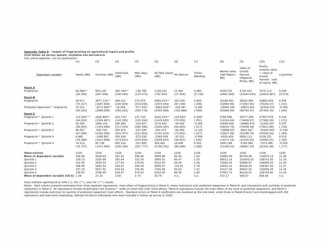
(Full follow-up survey sample, including non-borrowers)(For online appendix; not for publication)

(1) (2) (3) (4) (5) (6) (7) (8) (9) (10) (11)

Dependent variable: Seeds (MK) Fertilizer (MK) Chemicals (MK)

Man-days (MK)

All Paid Inputs (MK) KG Manure Times

Weeding

Market sales (Self Report, MK)

Value of Unsold Harvest (Regional Prices, MK)

Profits (market sales + value of unsold harvest - cost of inputs, MK)

Ln(profits)

Panel AFingerprint 60.585** 920.128 282.100** -136.780 1126.032 11.992 0.080 4228.220 4734.442 7570.113 0.039

(29.350) (667.006) (106.284) (115.473) (792.932) (27.904) (0.135) (4962.283) (23344.030) (24615.887) (0.079)Panel BFingerprint 49.011 3977.114** 296.011 272.076 4594.213** 122.326 0.365 23198.561 28031.981 43860.629 0.255

(72.217) (1687.829) (220.025) (210.036) (1874.643) (87.106) (.328) (16993.96) (71967.95) (76156.27) (.215)Predicted repayment * fingerprint 15.221 -4271.866** -19.358 -577.541* -4853.543** -154.387 -0.400 -26665.392 -33873.351 -52029.370 -0.305

(94.333) (2099.599) (295.322) (305.778) (2400.958) (105.886) (.439) (20686.96) (80794.67) (87493.76) (.245)Panel CFingerprint * Quintile 1 113.462*** 2636.880** 264.742* 147.140 3162.224** 118.604* 0.468* 9768.595 52077.286 57907.978 0.129

(44.024) (1304.867) (142.305) (121.034) (1415.625) (70.055) (.251) (13316.04) (74406.57) (77360.26) (.171)Fingerprint * Quintile 2 50.930 1956.152 285.580 -115.827 2176.834 -49.929 -0.368 24668.058 -39885.974 -21083.297 0.197 (59.562) (1453.069) (212.523) (280.486) (1635.342) (69.820) (.317) (18019.75) (76408.28) (79611.89) (.216)Fingerprint * Quintile 3 86.537 -593.742 353.570 -237.639 -391.274 -56.392 -0.123 -20898.037 -9621.667 -25345.653 -0.193

(67.608) (1452.306) (251.477) (311.853) (1701.534) (73.851) (.317) (13647.96) (51298.79) (54260.54) (.186)Fingerprint * Quintile 4 6.885 -1049.852 250.558 -573.530 -1365.938 -32.321 -0.056 -4020.628 5859.113 5128.222 0.019

(78.286) (1612.908) (273.541) (370.818) (2028.824) (68.537) (.346) (12271.19) (41342.84) (44092.51) (.190)Fingerprint * Quintile 5 76.413 85.736 305.314 -157.983 309.481 16.648 0.352 1890.188 -5784.984 -7574.496 -0.050

Appendix Table 6: Impact of fingerprinting on agricultural inputs and profits

(79.747) (1474.584) (240.184) (327.777) (1796.701) (80.069) (.336) (12186.01) (56867.20) (61201.66) (.177)

Observations 1226 1226 1226 1226 1226 1226 1226 1226 1226 1226 1226Mean of dependent variable 185.56 3948.93 362.92 396.56 4893.98 83.63 1.54 53965.29 86793.08 119870.13 11.28Quintile 1 129.13 2335.99 182.64 152.25 2800.01 85.47 1.20 48912.14 103543.10 138101.00 11.23Quintile 2 132.03 2924.01 277.92 178.55 3512.50 59.29 1.28 70582.23 60989.97 109699.20 11.33Quintile 3 198.08 5481.54 426.67 593.28 6699.57 125.01 1.78 44931.14 86190.55 108497.00 11.27Quintile 4 237.16 5837.92 543.52 726.95 7345.56 83.53 1.91 54127.28 98467.02 125928.20 11.34Quintile 5 239.52 4786.95 516.97 579.91 6123.35 80.35 1.83 47991.75 84126.01 109740.80 11.26Mean of dependent variable (US $) 1.28 27.23 2.50 2.73 33.75 n.a. n.a. 372.17 598.57 826.69 n.a.

Notes: Each column presents estimates from three separate regressions: main effect of fingerprinting in Panel A, linear interaction with predicted repayment in Panel B, and interactions with quintiles of predicted repayment in Panel C. All regressions include stratification cell (location * week of initial club visit) fixed effects. Panel B regressions include the main effect of the level of predicted repayment, and Panel C regressions include dummies for quintile of predicted repayment main effects. Standard errors on Panel A coefficients are clustered at the club level, while those in Panels B and C are bootstrapped with 200 replications and club-level resampling. Sample limited to individuals who were included in follow-up survey in 2009.

Stars indicate significance at 10% (*), 5% (**), and 1% (***) levels.

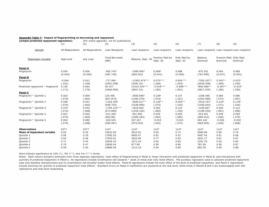
(For online appendix; not for publication)(1) (2) (3) (4) (5) (6) (7) (8) (9)

Sample: All Respondents All Respondents Loan Recipients Loan recipients Loan recipients Loan recipients Loan recipients Loan recipient Loan recipients

Dependent variable: Approved Any Loan Total Borrowed (MK) Balance, Sept. 30 Fraction Paid by

Sept. 30Fully Paid by Sept. 30

Balance, Eventual

Fraction Paid, Eventual

Fully Paid, Eventual

Panel AFingerprint 0.045 0.056 -692.743* -1489.945* 0.069* 0.088 -975.181 0.044 0.080

(0.054) (0.045) (381.745) (836.931) (0.041) (0.066) (762.090) (0.037) (0.061)Panel BFingerprint -0.064 0.012 -717.084 -11562.473*** 0.570*** 0.654*** -7303.437** 0.342** 0.423*

(.151) (.146) (2351.208) (3481.01) (.168) (.243) (3428.208) (.169) (.230)Predicted repayment * fingerprint 0.135 0.054 30.107 12415.234*** -0.618*** -0.698*** 7800.066** -0.367** -0.423*

(.171) (.176) (2656.956) (3947.51) (.185) (.261) (3817.025) (.185) (.246)Panel CFingerprint * Quintile 1 0.023 0.069 125.465 -2550.686* 0.138* 0.147 -1258.495 0.065 0.086

(.073) (.062) (837.873) (1494.379) (.076) (.101) (1454.586) (.074) (.097)Fingerprint * Quintile 2 0.036 0.041 -1193.165* -3306.017** 0.149** 0.204** -2516.761* 0.120* 0.178* (.070) (.063) (699.703) (1538.999) (.075) (.102) (1456.644) (.071) (.100)Fingerprint * Quintile 3 0.076 0.032 -1790.115*** -1819.843 0.060 0.110 -1190.697 0.026 0.112

(.070) (.068) (673.809) (1259.105) (.065) (.100) (1198.203) (.061) (.096)Fingerprint * Quintile 4 0.031 0.053 -311.359 -391.905 0.026 0.003 -423.401 0.028 0.039

(.070) (.063) (663.88) (1089.182) (.054) (.085) (969.012) (.048) (.075)Fingerprint * Quintile 5 0.054 0.085 -263.503 337.027 -0.013 -0.010 304.142 -0.006 -0.002 (.070) (.068) (590.087) (979.543) (.044) (.072) (893.653) (.040) (.068)

Observations 3277 3277 1147 1147 1147 1147 1147 1147 1147Mean of dependent variable 0.63 0.35 16912.60 2912.91 0.84 0.74 2080.86 0.89 0.79Quintile 1 0.58 0.29 17992.53 6955.67 0.62 0.52 4087.04 0.81 0.68Quintile 2 0.64 0.36 17870.61 4024.05 0.77 0.63 3331.17 0.81 0.67Quintile 3 0.71 0.44 16035.10 1571.44 0.92 0.83 1301.79 0.93 0.84Quintile 4 0.70 0.47 15805.54 877.80 0.95 0.85 781.59 0.95 0.87Quintile 5 0.59 0.30 16886.56 1214.19 0.94 0.85 950.29 0.95 0.88

(simple predicted repayment regression)Appendix Table 7: Impact of fingerprinting on borrowing and repayment

Notes: Each column presents estimates from three separate regressions: main effect of fingerprinting in Panel A, linear interaction with predicted repayment in Panel B, and interactions with quintiles of predicted repayment in Panel C. All regressions include stratification cell (location * week of initial club visit) fixed effects. The auxiliary regression used to calculate predicted repayment uses only baseline characteristics and no stratification cell (locality*week) fixed effects. Panel B regressions include the main effect of the level of predicted repayment, and Panel C regressions include dummies for quintile of predicted repayment main effects. Standard errors on Panel A coefficients are clustered at the club level, while those in Panels B and C are bootstrapped with 200 replications and club-level resampling.

Stars indicate significance at 10% (*), 5% (**), and 1% (***) levels.

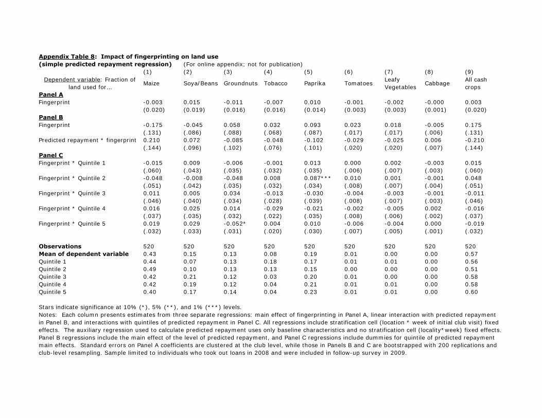
(For online appendix; not for publication)(1) (2) (3) (4) (5) (6) (7) (8) (9)

Dependent variable: Fraction of land used for… Maize Soya/Beans Groundnuts Tobacco Paprika Tomatoes Leafy

Vegetables Cabbage All cash crops

Panel AFingerprint -0.003 0.015 -0.011 -0.007 0.010 -0.001 -0.002 -0.000 0.003

(0.020) (0.019) (0.016) (0.016) (0.014) (0.003) (0.003) (0.001) (0.020)Panel BFingerprint -0.175 -0.045 0.058 0.032 0.093 0.023 0.018 -0.005 0.175

(.131) (.086) (.088) (.068) (.087) (.017) (.017) (.006) (.131)Predicted repayment * fingerprint 0.210 0.072 -0.085 -0.048 -0.102 -0.029 -0.025 0.006 -0.210

(.144) (.096) (.102) (.076) (.101) (.020) (.020) (.007) (.144)Panel CFingerprint * Quintile 1 -0.015 0.009 -0.006 -0.001 0.013 0.000 0.002 -0.003 0.015

(.060) (.043) (.035) (.032) (.035) (.006) (.007) (.003) (.060)Fingerprint * Quintile 2 -0.048 -0.008 -0.048 0.008 0.087*** 0.010 0.001 -0.001 0.048 (.051) (.042) (.035) (.032) (.034) (.008) (.007) (.004) (.051)Fingerprint * Quintile 3 0.011 0.005 0.034 -0.013 -0.030 -0.004 -0.003 -0.001 -0.011

(.046) (.040) (.034) (.028) (.039) (.008) (.007) (.003) (.046)Fingerprint * Quintile 4 0.016 0.025 0.014 -0.029 -0.021 -0.002 -0.005 0.002 -0.016

(.037) (.035) (.032) (.022) (.035) (.008) (.006) (.002) (.037)Fingerprint * Quintile 5 0.019 0.029 -0.052* 0.004 0.010 -0.006 -0.004 0.000 -0.019 (.032) (.033) (.031) (.020) (.030) (.007) (.005) (.001) (.032)

Observations 520 520 520 520 520 520 520 520 520Mean of dependent variable 0.43 0.15 0.13 0.08 0.19 0.01 0.00 0.00 0.57Quintile 1 0.44 0.07 0.13 0.18 0.17 0.01 0.01 0.00 0.56Quintile 2 0.49 0.10 0.13 0.13 0.15 0.00 0.00 0.00 0.51Quintile 3 0.42 0.21 0.12 0.03 0.20 0.01 0.00 0.00 0.58Quintile 4 0.42 0.19 0.12 0.04 0.21 0.01 0.01 0.00 0.58Quintile 5 0.40 0.17 0.14 0.04 0.23 0.01 0.01 0.00 0.60

Notes: Each column presents estimates from three separate regressions: main effect of fingerprinting in Panel A, linear interaction with predicted repayment in Panel B, and interactions with quintiles of predicted repayment in Panel C. All regressions include stratification cell (location * week of initial club visit) fixed effects. The auxiliary regression used to calculate predicted repayment uses only baseline characteristics and no stratification cell (locality*week) fixed effects. Panel B regressions include the main effect of the level of predicted repayment, and Panel C regressions include dummies for quintile of predicted repayment main effects. Standard errors on Panel A coefficients are clustered at the club level, while those in Panels B and C are bootstrapped with 200 replications and club-level resampling. Sample limited to individuals who took out loans in 2008 and were included in follow-up survey in 2009.

Appendix Table 8: Impact of fingerprinting on land use(simple predicted repayment regression)

Stars indicate significance at 10% (*), 5% (**), and 1% (***) levels.

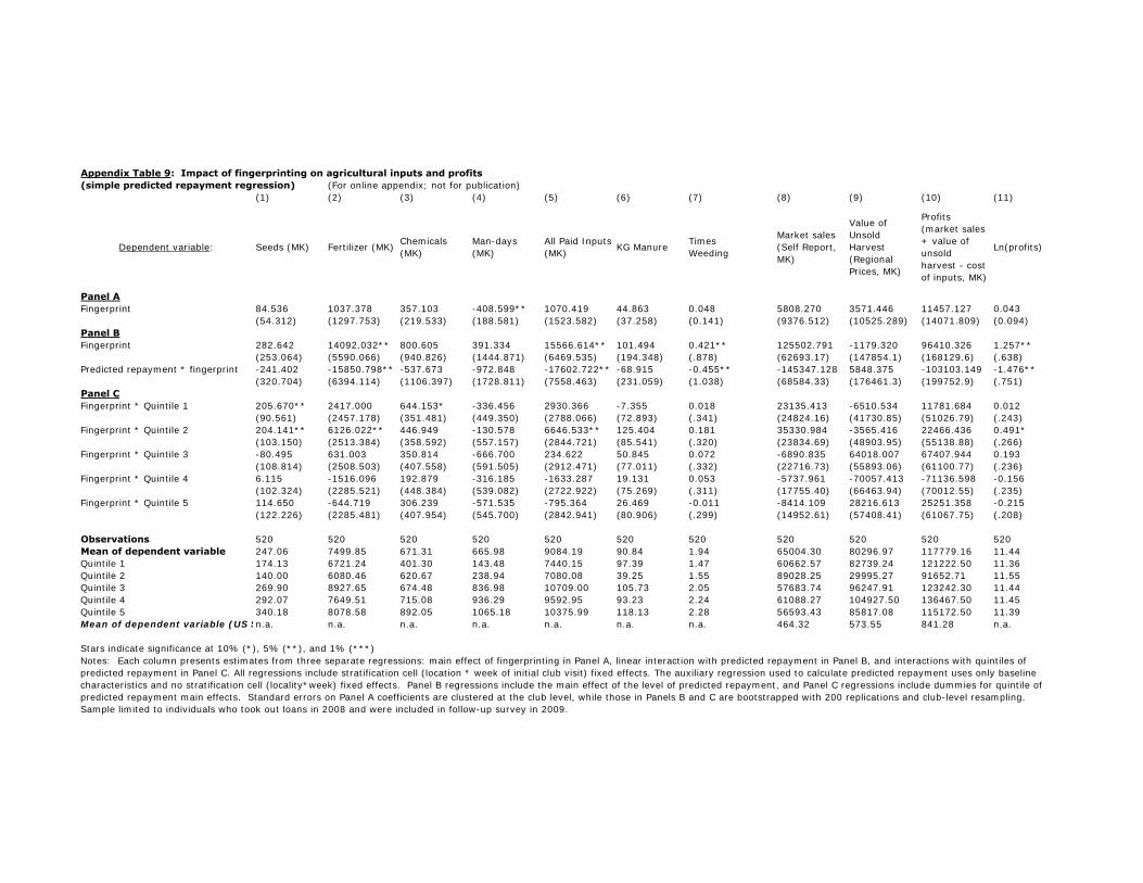
(1) (2) (3) (4) (5) (6) (7) (8) (9) (10) (11)

Dependent variable: Seeds (MK) Fertilizer (MK) Chemicals (MK)

Man-days (MK)

All Paid Inputs (MK) KG Manure Times

Weeding

Market sales (Self Report, MK)

Value of Unsold Harvest (Regional Prices, MK)

Profits (market sales + value of unsold harvest - cost of inputs, MK)

Ln(profits)

Panel AFingerprint 84.536 1037.378 357.103 -408.599** 1070.419 44.863 0.048 5808.270 3571.446 11457.127 0.043

(54.312) (1297.753) (219.533) (188.581) (1523.582) (37.258) (0.141) (9376.512) (10525.289) (14071.809) (0.094)Panel BFingerprint 282.642 14092.032** 800.605 391.334 15566.614** 101.494 0.421** 125502.791 -1179.320 96410.326 1.257**

(253.064) (5590.066) (940.826) (1444.871) (6469.535) (194.348) (.878) (62693.17) (147854.1) (168129.6) (.638)Predicted repayment * fingerprint -241.402 -15850.798** -537.673 -972.848 -17602.722** -68.915 -0.455** -145347.128 5848.375 -103103.149 -1.476**

(320.704) (6394.114) (1106.397) (1728.811) (7558.463) (231.059) (1.038) (68584.33) (176461.3) (199752.9) (.751)Panel CFingerprint * Quintile 1 205.670** 2417.000 644.153* -336.456 2930.366 -7.355 0.018 23135.413 -6510.534 11781.684 0.012

(90.561) (2457.178) (351.481) (449.350) (2788.066) (72.893) (.341) (24824.16) (41730.85) (51026.79) (.243)Fingerprint * Quintile 2 204.141** 6126.022** 446.949 -130.578 6646.533** 125.404 0.181 35330.984 -3565.416 22466.436 0.491* (103.150) (2513.384) (358.592) (557.157) (2844.721) (85.541) (.320) (23834.69) (48903.95) (55138.88) (.266)Fingerprint * Quintile 3 -80.495 631.003 350.814 -666.700 234.622 50.845 0.072 -6890.835 64018.007 67407.944 0.193

(108.814) (2508.503) (407.558) (591.505) (2912.471) (77.011) (.332) (22716.73) (55893.06) (61100.77) (.236)Fingerprint * Quintile 4 6.115 -1516.096 192.879 -316.185 -1633.287 19.131 0.053 -5737.961 -70057.413 -71136.598 -0.156

(102.324) (2285.521) (448.384) (539.082) (2722.922) (75.269) (.311) (17755.40) (66463.94) (70012.55) (.235)Fingerprint * Quintile 5 114.650 -644.719 306.239 -571.535 -795.364 26.469 -0.011 -8414.109 28216.613 25251.358 -0.215 (122.226) (2285.481) (407.954) (545.700) (2842.941) (80.906) (.299) (14952.61) (57408.41) (61067.75) (.208)

Observations 520 520 520 520 520 520 520 520 520 520 520Mean of dependent variable 247.06 7499.85 671.31 665.98 9084.19 90.84 1.94 65004.30 80296.97 117779.16 11.44Quintile 1 174.13 6721.24 401.30 143.48 7440.15 97.39 1.47 60662.57 82739.24 121222.50 11.36Quintile 2 140.00 6080.46 620.67 238.94 7080.08 39.25 1.55 89028.25 29995.27 91652.71 11.55Quintile 3 269.90 8927.65 674.48 836.98 10709.00 105.73 2.05 57683.74 96247.91 123242.30 11.44Quintile 4 292.07 7649.51 715.08 936.29 9592.95 93.23 2.24 61088.27 104927.50 136467.50 11.45Quintile 5 340.18 8078.58 892.05 1065.18 10375.99 118.13 2.28 56593.43 85817.08 115172.50 11.39Mean of dependent variable (US $n.a. n.a. n.a. n.a. n.a. n.a. n.a. 464.32 573.55 841.28 n.a.

Appendix Table 9: Impact of fingerprinting on agricultural inputs and profits(simple predicted repayment regression) (For online appendix; not for publication)

Stars indicate significance at 10% (*), 5% (**), and 1% (***) Notes: Each column presents estimates from three separate regressions: main effect of fingerprinting in Panel A, linear interaction with predicted repayment in Panel B, and interactions with quintiles of predicted repayment in Panel C. All regressions include stratification cell (location * week of initial club visit) fixed effects. The auxiliary regression used to calculate predicted repayment uses only baseline characteristics and no stratification cell (locality*week) fixed effects. Panel B regressions include the main effect of the level of predicted repayment, and Panel C regressions include dummies for quintile of predicted repayment main effects. Standard errors on Panel A coefficients are clustered at the club level, while those in Panels B and C are bootstrapped with 200 replications and club-level resampling. Sample limited to individuals who took out loans in 2008 and were included in follow-up survey in 2009.

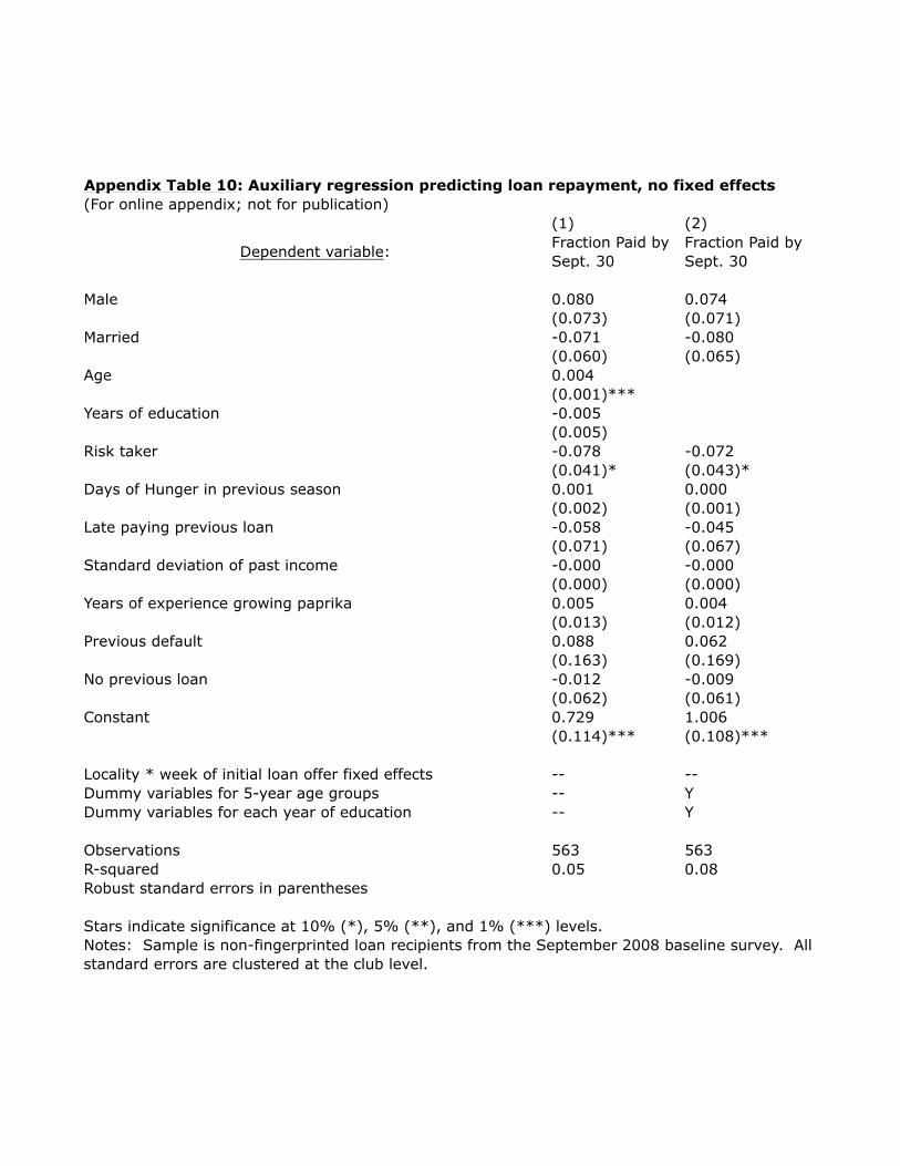
(For online appendix; not for publication)

(1) (2)

Dependent variable:Fraction Paid by

Sept. 30

Fraction Paid by

Sept. 30

Male 0.080 0.074

(0.073) (0.071)

Married -0.071 -0.080

(0.060) (0.065)

Age 0.004

(0.001)***

Years of education -0.005

(0.005)

Risk taker -0.078 -0.072

(0.041)* (0.043)*

Days of Hunger in previous season 0.001 0.000

(0.002) (0.001)

Late paying previous loan -0.058 -0.045

(0.071) (0.067)

Standard deviation of past income -0.000 -0.000

(0.000) (0.000)

Years of experience growing paprika 0.005 0.004

(0.013) (0.012)

Previous default 0.088 0.062

(0.163) (0.169)

No previous loan -0.012 -0.009

(0.062) (0.061)

Constant 0.729 1.006

(0.114)*** (0.108)***

Locality * week of initial loan offer fixed effects -- --

Dummy variables for 5-year age groups -- Y

Dummy variables for each year of education -- Y

Observations 563 563

R-squared 0.05 0.08

Appendix Table 10: Auxiliary regression predicting loan repayment, no fixed effects

Robust standard errors in parentheses

Notes: Sample is non-fingerprinted loan recipients from the September 2008 baseline survey. All

standard errors are clustered at the club level.

Stars indicate significance at 10% (*), 5% (**), and 1% (***) levels.

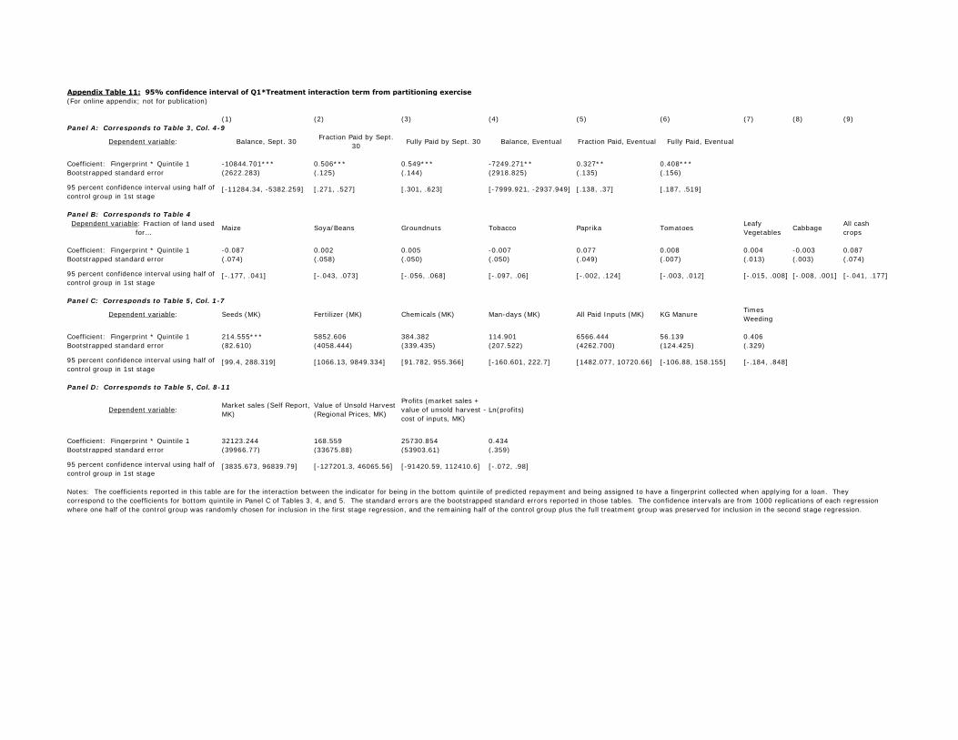
(For online appendix; not for publication)

(1) (2) (3) (4) (5) (6) (7) (8) (9)Panel A: Corresponds to Table 3, Col. 4-9

Dependent variable: Balance, Sept. 30 Fraction Paid by Sept. 30 Fully Paid by Sept. 30 Balance, Eventual Fraction Paid, Eventual Fully Paid, Eventual

Coefficient: Fingerprint * Quintile 1 -10844.701*** 0.506*** 0.549*** -7249.271** 0.327** 0.408***Bootstrapped standard error (2622.283) (.125) (.144) (2918.825) (.135) (.156)

95 percent confidence interval using half of control group in 1st stage

[-11284.34, -5382.259] [.271, .527] [.301, .623] [-7999.921, -2937.949] [.138, .37] [.187, .519]

Panel B: Corresponds to Table 4Dependent variable: Fraction of land used

for… Maize Soya/Beans Groundnuts Tobacco Paprika Tomatoes Leafy Vegetables Cabbage All cash

crops

Coefficient: Fingerprint * Quintile 1 -0.087 0.002 0.005 -0.007 0.077 0.008 0.004 -0.003 0.087Bootstrapped standard error (.074) (.058) (.050) (.050) (.049) (.007) (.013) (.003) (.074)

95 percent confidence interval using half of control group in 1st stage

[-.177, .041] [-.043, .073] [-.056, .068] [-.097, .06] [-.002, .124] [-.003, .012] [-.015, .008] [-.008, .001] [-.041, .177]

Panel C: Corresponds to Table 5, Col. 1-7

Dependent variable: Seeds (MK) Fertilizer (MK) Chemicals (MK) Man-days (MK) All Paid Inputs (MK) KG Manure Times Weeding

Coefficient: Fingerprint * Quintile 1 214.555*** 5852.606 384.382 114.901 6566.444 56.139 0.406Bootstrapped standard error (82.610) (4058.444) (339.435) (207.522) (4262.700) (124.425) (.329)

95 percent confidence interval using half of control group in 1st stage

[99.4, 288.319] [1066.13, 9849.334] [91.782, 955.366] [-160.601, 222.7] [1482.077, 10720.66] [-106.88, 158.155] [-.184, .848]

Panel D: Corresponds to Table 5, Col. 8-11

Dependent variable: Market sales (Self Report, MK)

Value of Unsold Harvest (Regional Prices, MK)

Profits (market sales + value of unsold harvest - cost of inputs, MK)

Ln(profits)

Coefficient: Fingerprint * Quintile 1 32123.244 168.559 25730.854 0.434Bootstrapped standard error (39966.77) (33675.88) (53903.61) (.359)

95 percent confidence interval using half of control group in 1st stage

[3835.673, 96839.79] [-127201.3, 46065.56] [-91420.59, 112410.6] [-.072, .98]

Notes: The coefficients reported in this table are for the interaction between the indicator for being in the bottom quintile of predicted repayment and being assigned to have a fingerprint collected when applying for a loan. They correspond to the coefficients for bottom quintile in Panel C of Tables 3, 4, and 5. The standard errors are the bootstrapped standard errors reported in those tables. The confidence intervals are from 1000 replications of each regression where one half of the control group was randomly chosen for inclusion in the first stage regression, and the remaining half of the control group plus the full treatment group was preserved for inclusion in the second stage regression.

Appendix Table 11: 95% confidence interval of Q1*Treatment interaction term from partitioning exercise

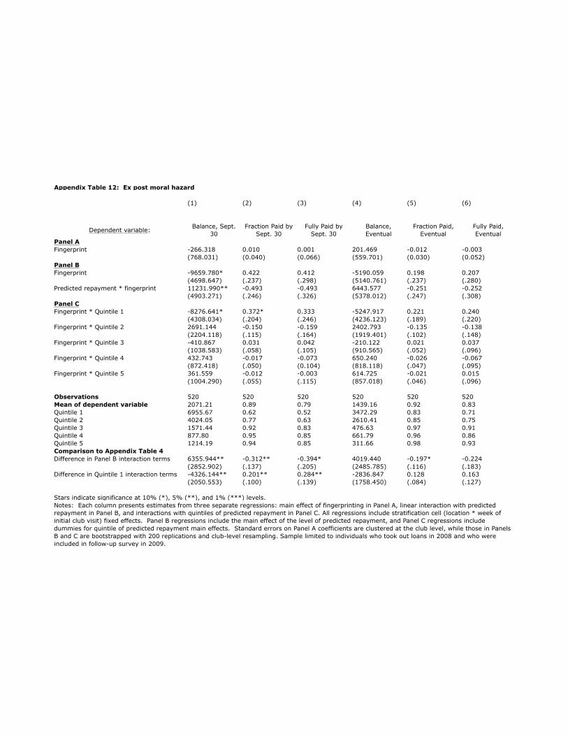
(1) (2) (3) (4) (5) (6)

Dependent variable:Balance, Sept.

30

Fraction Paid by

Sept. 30

Fully Paid by

Sept. 30

Balance,

Eventual

Fraction Paid,

Eventual

Fully Paid,

Eventual

Panel A

Fingerprint -266.318 0.010 0.001 201.469 -0.012 -0.003

(768.031) (0.040) (0.066) (559.701) (0.030) (0.052)

Panel B

Fingerprint -9659.780* 0.422 0.412 -5190.059 0.198 0.207

(4698.647) (.237) (.298) (5140.761) (.237) (.280)

Predicted repayment * fingerprint 11231.990** -0.493 -0.493 6443.577 -0.251 -0.252

(4903.271) (.246) (.326) (5378.012) (.247) (.308)

Panel C

Fingerprint * Quintile 1 -8276.641* 0.372* 0.333 -5247.917 0.221 0.240

(4308.034) (.204) (.246) (4236.123) (.189) (.220)

Fingerprint * Quintile 2 2691.144 -0.150 -0.159 2402.793 -0.135 -0.138

(2204.118) (.115) (.164) (1919.401) (.102) (.148)

Fingerprint * Quintile 3 -410.867 0.031 0.042 -210.122 0.021 0.037

(1038.583) (.058) (.105) (910.565) (.052) (.096)

Fingerprint * Quintile 4 432.743 -0.017 -0.073 650.240 -0.026 -0.067

(872.418) (.050) (0.104) (818.118) (.047) (.095)

Fingerprint * Quintile 5 361.559 -0.012 -0.003 614.725 -0.021 0.015

(1004.290) (.055) (.115) (857.018) (.046) (.096)

Observations 520 520 520 520 520 520

Mean of dependent variable 2071.21 0.89 0.79 1439.16 0.92 0.83

Quintile 1 6955.67 0.62 0.52 3472.29 0.83 0.71

Quintile 2 4024.05 0.77 0.63 2610.41 0.85 0.75

Quintile 3 1571.44 0.92 0.83 476.63 0.97 0.91

Quintile 4 877.80 0.95 0.85 661.79 0.96 0.86

Quintile 5 1214.19 0.94 0.85 311.66 0.98 0.93

Comparison to Appendix Table 4

Difference in Panel B interaction terms 6355.944** -0.312** -0.394* 4019.440 -0.197* -0.224

(2852.902) (.137) (.205) (2485.785) (.116) (.183)

Difference in Quintile 1 interaction terms -4326.144** 0.201** 0.284** -2836.847 0.128 0.163

(2050.553) (.100) (.139) (1758.450) (.084) (.127)

Stars indicate significance at 10% (*), 5% (**), and 1% (***) levels.

Appendix Table 12: Ex post moral hazard

Notes: Each column presents estimates from three separate regressions: main effect of fingerprinting in Panel A, linear interaction with predicted

repayment in Panel B, and interactions with quintiles of predicted repayment in Panel C. All regressions include stratification cell (location * week of

initial club visit) fixed effects. Panel B regressions include the main effect of the level of predicted repayment, and Panel C regressions include

dummies for quintile of predicted repayment main effects. Standard errors on Panel A coefficients are clustered at the club level, while those in Panels

B and C are bootstrapped with 200 replications and club-level resampling. Sample limited to individuals who took out loans in 2008 and who were

included in follow-up survey in 2009.

(a) Increase in repayment due to fingerprinting in Quintile 1 4,905.00 Malawi kwacha(b) Quintile 1 as share of all borrowers 20.0%(c) Borrowers as share of all fingerprinted 50%

(d) Total benefit per individual fingerprinted [ = (a)*(b)*(c)] 490.50 Malawi kwacha

(e) Cost per equipment unit 101,500 Malawi kwacha(f) Equipment amortization period 3 years(g) Annual equipment amortization [ = (e) / (f)] 33,833 (h) Fingerprinted individuals per equipment unit 417 individuals(i) Equipment cost per farmer [ = (g) / (h)] 81.20 Malawi kwacha(j) Loan officer time cost per farmer 19.25 Malawi kwacha(k) Transaction cost per fingerprint checked 108.75 Malawi kwacha

(l) Total cost per individual fingerprinted [ = (i) + (j) + (k)] 209.20 Malawi kwacha

281.30 Malawi kwacha2.34

145 MK/US$15,000 Malawi kwacha32.7%

700 USD12

5,000

5 minutes40,000 Malawi kwacha

173.2 hours

Fingerprinting time per individualMonthly salary of MRFC loan officerHours worked per month by MFRC loan officer

Exchange rate:Loan sizeIncrease in share of loan repaid due to fingerprinting in Quint

Cost per equipment unit (laptop computer + fingerprint scanNumber of equipment unitsNew loan applicants fingerprinted per year

Assumptions:

Appendix Table 13: Benefit-cost analysis

Benefit

Cost

(m) Net benefit per fingerprinted farmer [ = (d) - (l)](n) Benefit-cost ratio [ = (d) / (l)]

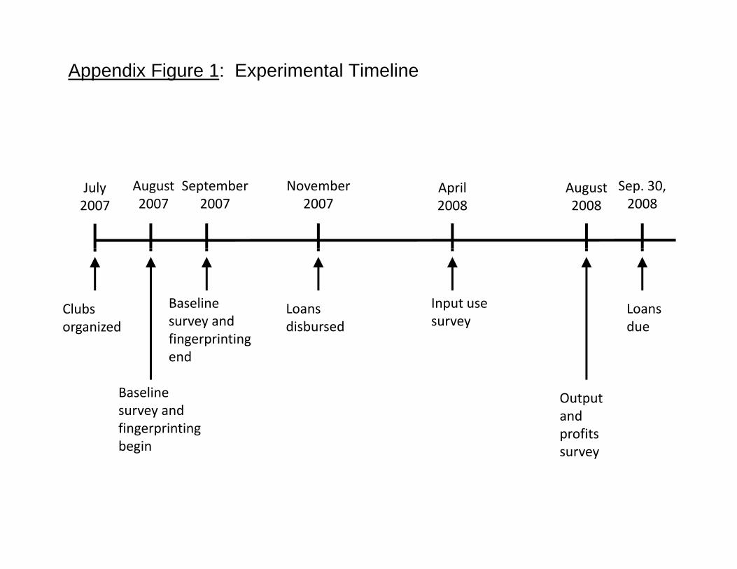
Appendix Figure 1: Experimental Timeline

July 2007

August 2007

Sep. 30, 2008

November 2007

April 2008

September 2007

August2008

Clubs  Loans  Loans Input use survey

Baseline survey andorganized

Baseline

disbursed duesurveysurvey and fingerprinting end

Baseline survey and fingerprinting begin

Output and profits survey

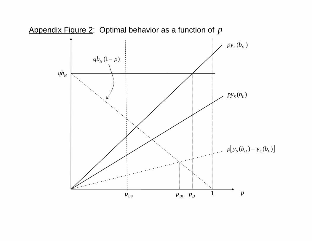
)(bpy

Appendix Figure 2: Optimal behavior as a function of p

)( HS bpy

Hqb

)1( pqbH

)( LS bpy

Hqb

)()( LSHS bybyp

p1Dp0Bp 1Bp Dp0Bp 1Bp

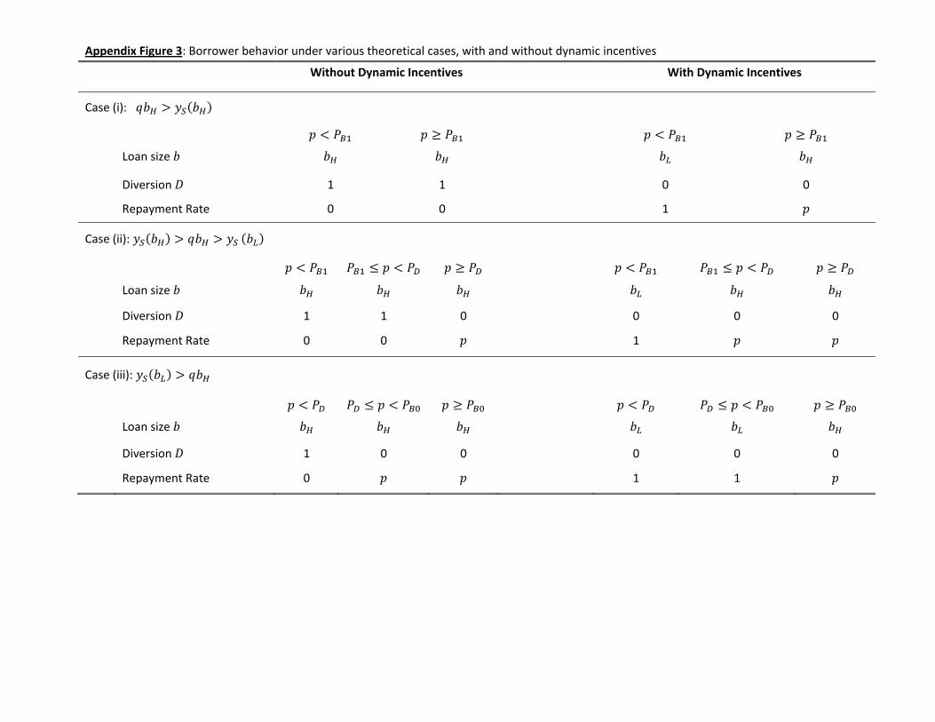
Appendix Figure 3: Borrower behavior under various theoretical cases, with and without dynamic incentives 

 

 

  Without Dynamic Incentives    With Dynamic Incentives 

Case (i):     

           

  Loan size     

  Diversion    1  1    0  0 

  Repayment Rate  0  0    1 

Case (ii):     

               

  Loan size     

  Diversion    1  1  0    0  0  0 

  Repayment Rate  0  0    1 

Case (iii):   

               

  Loan size     

  Diversion    1  0  0    0  0  0 

  Repayment Rate  0    1  1