Embed Size (px)
Citation preview

NBER WORKING PAPER SERIES
THE CONSEQUENCES OF MORTGAGE CREDIT EXPANSION:EVIDENCE FROM THE 2007 MORTGAGE DEFAULT CRISIS
Atif MianAmir Sufi
Working Paper 13936http://www.nber.org/papers/w13936
NATIONAL BUREAU OF ECONOMIC RESEARCH1050 Massachusetts Avenue
Cambridge, MA 02138April 2008
We gratefully acknowledge financial support from the Initiative on Global Markets at the Universityof Chicago Graduate School of Business and the IBM Corporation. The data analysis was made possibleby the generous help of Myra Hart (Equifax Predictive Services), Jim DiSalvo (Philadelphia Fed),Robert Shiller, Cameron Rogers (Fiserv), Greg Runk (CapIndex), and David Stiff (Fiserv). We thankMitch Berlin, Jonathan Guryan, Bob Hunt, Erik Hurst, Doug Diamond, Raghu Rajan, Josh Rauh, andparticipants at the Chicago GSB finance lunch, Chicago GSB applied economics lunch, Emory University,and the Federal Reserve Bank of Philadelphia for comments and feedback. We also thank Sim Wee,Rafi Nulman, and Smitha Nagaraja for excellent research assistance. The views expressed hereinare those of the author(s) and do not necessarily reflect the views of the National Bureau of EconomicResearch.
NBER working papers are circulated for discussion and comment purposes. They have not been peer-reviewed or been subject to the review by the NBER Board of Directors that accompanies officialNBER publications.
© 2008 by Atif Mian and Amir Sufi. All rights reserved. Short sections of text, not to exceed two paragraphs,may be quoted without explicit permission provided that full credit, including © notice, is given tothe source.

The Consequences of Mortgage Credit Expansion: Evidence from the 2007 Mortgage DefaultCrisisAtif Mian and Amir SufiNBER Working Paper No. 13936April 2008JEL No. E44,E51,G21,L85,O51,R21
ABSTRACT
We demonstrate that a rapid expansion in the supply of mortgages driven by disintermediation explainsa large fraction of recent U.S. house price appreciation and subsequent mortgage defaults. We identifythe effect of shifts in the supply of mortgage credit by exploiting within-county variation across zipcodes that differed in latent demand for mortgages in the mid 1990s. From 2001 to 2005, high latentdemand zip codes experienced large relative decreases in denial rates, increases in mortgages originated,and increases in house price appreciation, despite the fact that these zip codes experienced significantlynegative relative income and employment growth over this time period. These patterns for high latentdemand zip codes were driven by a sharp relative increase in the fraction of loans sold by originatorsshortly after origination, a process which we refer to as "disintermediation." The increase in disintermediation-drivenmortgage supply to high latent demand zip codes from 2001 to 2005 led to subsequent large increasesin mortgage defaults from 2005 to 2007. Our results suggest that moral hazard on behalf of originatorsselling mortgages is a main culprit for the U.S. mortgage default crisis.
Atif MianUniversity of ChicagoGraduate School of Business5807 South Woodlawn AvenueChicago, IL 60637and [email protected]
Amir SufiUniversity of ChicagoGraduate School of Business5807 South Woodlawn AvneueChicago, IL [email protected]

1
Recent developments in the U.S. housing market are the focus of increased anxiety among
policy-makers, investors, and financial markets. After experiencing a dramatic rise in house
prices and outstanding mortgage debt, the U.S. has experienced a sharp increase in mortgage
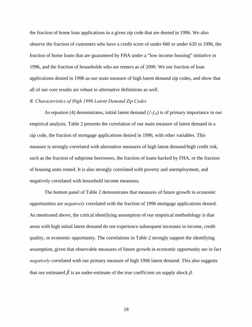
defaults. Figure 1A shows that the average house price in the U.S increased by almost 200%
from 1996 to 2005. Figure 1B demonstrates a similar rise in outstanding mortgage debt, and also
that the rise in mortgage debt has been significantly larger than the rise in other types of
consumer debt. Figure 1C shows that the total number of accepted mortgage applications for new
home purchase increased rapidly from 2003 to 2005, suggesting the entry of new consumers in
this market during this time period.
The rapid growth in mortgage credit and house prices has given way to grave concerns as
mortgage defaults continue to mount. For example, default rates rose by over 50% between the
fourth quarter of 2005 and the second quarter of 2007 (Figure 1D). The market value of
mortgage securities has fallen precipitously as well, with some tranches losing up to 70 to 80%
of their value in less than a year. Many believe that weakness in the U.S. housing market poses a
serious threat to financial markets and economic growth.1 The January 22nd, 2008 FOMC
statement justified a 75 basis point reduction in the federal funds rate in part because “…
incoming information indicates a deepening of the housing contraction …”
The goal of this paper is to investigate the cause of the sharp rise in house prices and
subsequent spike in mortgage default rates. Our central finding is that a rapid expansion in the
supply of credit to zip codes with high latent demand for mortgages is a main cause of both
house price appreciation from 2001 to 2005 and the subsequent sharp increase in defaults from
1 See Ng and Lauricella (WSJ, July 13th, 2007), Wessel (WSJ, September 13th, 2007), Lahart (August 27th, 2007), and Bater (WSJ, November 20th, 2007). Press articles refer to the current mortgage environment as a “mortgage crisis” (Creswell and Bajaj, NYT, March 5th, 2007) that “is comparable to some of the biggest financial disasters of the past half-century” (Ip, Whitehouse, and Lucchetti, WSJ, December 10th, 2007).

2
2005 to 2007. The expansion in credit supply was driven by a shift in the mortgage industry
towards “disintermediation”, which we define as the process in which originators sell mortgages
in the secondary market shortly after origination.
Our analysis is based on a new data set constructed from a number of proprietary and
public data sources. It represents one of the most comprehensive and disaggregated data sets in
the real estate and consumer credit literature. More specifically, our zip code-year level data set
covers 1996 through 2007 and includes a number of key variables of interest including
outstanding consumer debt of different types, defaults, house prices, mortgage loan application
characteristics, mortgage terms, and demographic variables such as income and crime. Given the
large number of zip codes in our sample, we are able to exploit cross-sectional variation over
time in zip code outcomes to empirically isolate our coefficients of interest.
We identify the causal effect of expansion in the supply of mortgage credit on subsequent
changes in loan originations, house prices, and defaults by exploiting within-county across-zip
code variation in initial latent demand for mortgages. Our primary measure of initial latent
demand is the fraction of mortgage applications denied by originating institutions in the zip code
in 1996.
The intuition behind our identification strategy can be understood through a simple
example. Consider two zip codes A and B that lie in the same county, but differ in the credit
worthiness of its households. In particular, suppose that all households in zip code A are
creditworthy enough to be given mortgages at the risk free rate. Everyone in zip code B also
applies for a mortgage loan, but only 50% of households have their applications accepted. The
remaining 50% are rejected due to a poor credit record. Then suppose there is an outward shift in
the supply of capital such that lenders are willing to lend to riskier households. Then, ceteris

3
paribus, zip code B that has high initial latent demand (i.e., unfulfilled demand) will experience a
sharp growth in credit, while zip code A will experience no change.2
The key identifying assumption in the example above is that initial 1996 latent demand
for loans in a zip code is not positively correlated with subsequent improvements in credit
quality. For example, if households in zip code B experience a greater increase in economic
opportunities than those in A, then credit growth in B may be attributed to the increase in credit
quality rather than an increase in supply. However, we show that in our context zip codes with
higher initial latent demand for mortgages experienced negative relative income and employment
growth from 2001 to 2005.
We implement this empirical strategy by first showing evidence of a shift in the supply of
mortgage credit toward high 1996 latent demand zip codes from 2001 to 2005. We demonstrate
that high 1996 latent demand zip codes experience a dramatic relative reduction in mortgage
denial rates during this time period. Simultaneous with the reduction in denial rates, high 1996
latent demand zip codes experience much larger increases in the debt to income ratio of accepted
mortgage applications. The source of this increase in credit availability is disintermediation: the
fraction of mortgages sold by originators in the secondary market experiences a sharp relative
increase for high latent demand zip codes from 2001 to 2005. Finally, the interest spread
between mortgages to low credit quality borrowers and high quality borrowers narrows to
historical lows during this period. Taken together, these facts demonstrate a sharp relative
increase in the supply of mortgages to high 1996 latent demand zip codes from 2001 to 2005.
We then show the effects of the credit expansion on originated mortgage amounts, house
price appreciation, and subsequent defaults. We find that high 1996 latent demand zip codes
experience a large relative increase in both mortgage debt and house prices from 2001 to 2005. 2 In Section III, we formalize this intuition in a simple Stiglitz and Weiss (1981) inspired model.

4
The relative increase in house prices in high 1996 latent demand zip codes occurs despite the fact
that these zip codes experience negative relative income and employment growth over this time
period. Our findings suggest that expansion in the supply of mortgage credit is a primary cause
of house price appreciation in high latent demand zip codes from 2001 to 2005.
The expansion in credit to high latent demand zip codes is followed by a large increase in
default rates. In terms of magnitudes, a one standard deviation increase in “supply-driven”
mortgage debt from 2001 to 2005 leads to a one-half standard deviation increase in mortgage
default rates from 2005 to 2007. Furthermore, a one standard deviation increase in supply-driven
house price appreciation leads to a two standard deviation increase in mortgage default rates.
Our findings demonstrate that the expansion in the supply of credit driven by
disintermediation is responsible for the rapid increase in new loan originations, house price
appreciation, and subsequent large increase in default rates. By allowing mortgage originators to
shed credit risk by selling loans, disintermediation significantly increased the amount of lending
to riskier borrowers. We directly link the disintermediation process to credit expansion, house
price appreciation, and ultimate defaults by showing that these changes take place in precisely
those zip codes that experienced the greatest increase in disintermediation. For example, credit
growth from 2001 to 2005 and growth in default rates from 2005 to 2007 is significantly higher
for zip codes with larger increases in disintermediation.
Furthermore, the positive relation between disintermediation and subsequent defaults is
concentrated in zip codes in which a larger fraction of loans were sold by originators to
unaffiliated, non-commercial bank institutions. In other words, disintermediation only leads to
higher default rates when originator incentives are less aligned with buyers and when the buying

5
institution has no specialized screening skills. Taken together, these findings suggest that moral
hazard on behalf of originators is a primary culprit for the default crisis.
Research presented here is related to recent working papers examining the rise in default
rates on subprime mortgages (Keys, Mukherjee, Seru and Vig (2008), Demyanyk and Van
Hemert (2007), and Doms, Furlong, and Krainer (2007)). Among these papers, the closest to
ours is Keys, Mukherjee, Seru and Vig (2008), who exploit credit score threshold rules used for
securitization to show that securitization leads to more defaults. Our work is also related to an
earlier strand of literature that examines the relation between housing price changes and
consumer borrowing (Poterba (1984), Case and Shiller (1989), Stein (1995), Genesove and
Mayer (1997, 2001), Hurst and Stafford (2004), Glaeser and Gyourko (2005), Himmelberg,
Mayer, and Sinai (2005), Brunnermeier and Julliard (2007)).
This paper makes a novel contribution to this literature on several dimensions. First, and
most important, we believe that our analysis is the first to demonstrate the causal effect of
mortgage credit expansion driven by disintermediation from 2001 to 2005 on house price
appreciation and subsequent defaults. We are able to demonstrate causality given our unique
empirical strategy that exploits within-county variation across zip codes in initial latent demand
for mortgages. In addition, our zip code data on income, employment, and crime allow us to
perform tests that mitigate concerns that omitted credit quality variables are polluting the
estimates of the supply effect.
Second, the data set we employ covers all major geographic areas of the United States.
As a result, we can utilize the microeconomic estimates to examine the macroeconomic effects
of supply expansion. Our conservative estimates based on the difference in difference within-
county estimator suggests that at least 15% of home purchase originations, and 10% of house

6
price appreciation from 2001 to 2005 can be attributed to credit supply expansion (see Section V
for details).
Third, the causal link we establish between credit supply, house prices, and subsequent
financial crisis is not an isolated incident. Reinhart and Rogoff (2008) document that a liquidity
and asset price boom followed by financial collapse and economic slowdown is a trademark of
crises in many developed countries, including Japan, Spain, UK, and Norway. Our findings
provide important microeconomic evidence on this broader phenomenon by documenting the
precise channel through which mortgage credit expansion in the U.S. caused a rapid appreciation
in house prices and a subsequent increase in mortgage defaults.
The rest of the paper proceeds as follows. The next section describes the data and
presents the summary statistics. Section II presents evidence of an aggregate shift in the supply
of mortgage credit from 2001 to 2005. Section III presents the empirical methodology, Section
IV presents the core results of our analysis, and Section V concludes.
I. Data and Summary Statistics
Our empirical analysis employs a unique zip code-year level panel data set with
information on outstanding consumer debt, consumer debt defaults, house prices, mortgage
terms, and demographic variables. There are three main data sources that comprise our final data
set: Equifax data on consumer credit, Fiserv Case Shiller Weiss data on house prices, and Home
Mortgage Disclosure Act (HMDA) data on loan terms. In addition, we obtain demographic
information from the Decennial 2000 Census, the Census Statistics of U.S. Businesses, the
Internal Revenue Service, and CAP Index Inc. Our final data set includes 2,920 zip codes from
1996 through 2007, and these zip codes represent more than 40% of outstanding consumer debt

7
in the United States. In this section, we explain the construction of the final data set and present
summary statistics.
A. Equifax Predictive Services Data
We collect data on outstanding consumer credit amounts and defaults from Equifax
Predictive Services. Equifax is a consumer credit rating agency that collects, organizes, and
manages credit information for U.S. consumers. The original Equifax data have credit
information for almost 170 million individuals going as far back as 1990. However, due to cost
and confidentiality concerns, Equifax aggregated the provided data at the zip code level at a
quarterly frequency from 1998Q1 to 2007Q2, and at an annual frequency from 1991 to 1997.
We therefore have aggregate debt composition and defaults of every U.S. zip code at a
quarterly frequency from 1998 through the second quarter of 2007, and at an annual frequency
from 1991 through 1997. The outstanding consumer credit and delinquency data at the zip code
level are broken down by type of consumer loans (credit cards, mortgages, home equity lines,
auto loans, etc.), as well as consumer credit score.
We construct aggregate measures of mortgage debt, home equity debt, and non-home
consumer debt. The latter category aggregates credit card debt, consumer loans, student loans,
and auto loans. The Equifax data record default amounts for the following varying degrees of
default: 30 days late, 60 days late, 90 days late, 120 days late or collections, severe derogatory,
and bankruptcy. In the analysis below, we define defaults as broadly as possible: default amounts
include any amounts 30 days late or more. The main reason for this choice is that many defaults
are recent. All of our specifications are run in first-differences, which mitigates concerns about
the average level of default for different default categories. Our results are materially unchanged
if we use an alternative definition of default such as 60 plus days late or more.

8
B. Home Mortgage Disclosure Act (HMDA) Data
While the Equifax data provide us a comprehensive picture of the stock of consumer
credit at the zip code level, they do not provide information on the flow of new mortgage and
home equity loans being originated. We therefore collect this information from loan origination
data sets collected under the “Home Mortgage Disclosure Act” (HMDA).
In order to supervise and enforce fair lending practices across that U.S., the U.S.
Congress mandates that all loans applications related to home purchase, refinancing, and home
improvement be reported to the federal government. The loan application information is publicly
available through HMDA from 1996 through 2006. For every loan application, the public data
record its status (denied / approved / originated), purpose (home purchase / refinancing / home
improvement), loan amount, and applicant characteristics including race, sex, income and home
ownership status. It also reports lender information, including the lender’s reasons for applicant
denial, type of lender, and whether the loan originator sold the loan to the secondary market
within a year. Since 2004, HMDA has also recorded the initial interest rate spread of loan
originations, and lien status. HMDA does not provide information on the maturity structure of a
loan, or whether the loan has a fixed rate mortgage or ARM. Nonetheless, with millions of loan
applications recorded every year, HMDA remains one of the best sources for understanding loan
origination patterns.
Since our unit of analysis is a zip code, we aggregate the application-level HMDA data to
census tracts, which are the smallest available geographical identifiers in the data. The census
tract level HMDA data are then aggregated into zip codes using the census tract to zip code
match provided by Geolytics. Census tracts are smaller than zip codes on average, with about
60,000 census tracts for approximately 40,000 zip codes. Consequently the quality of the match

9
from census tract to zip code is excellent. For example, 85% of matched census tracts in our final
sample have over 90% of their population living in the zip code to which they are matched. The
intersection of HMDA and Equifax data contains 19,368 zip codes.
C. Fiserv Case Shiller Weiss Data
Our primary data source for zip code level house price indices is Fiserv Case Shiller
Weiss. FCSW uses same house repeat sales data to construct house price indices at the zip code
level. The zip code level house price data we utilize in this study underlies the MSA level
S&P/Case Shiller indices, upon which futures are traded on the Chicago Mercantile Exchange.
The data set includes house price indices through the second quarter of 2007.
One limitation of the data is that FCSW require a significant number of transactions in a
given zip code to obtain reliable estimates of changes in house prices over time. As a result,
FCSW has house prices for only 3,056 of the zip codes in Equifax-HMDA sample. While FCSW
covers only 15% of the number of zip codes in the Equifax-Census sample, their indices are
constructed for all major metropolitan and highly populated zip codes in the United States. As a
result, our final sample includes over 40% of the aggregate outstanding amounts of consumer
debt, and almost 45% of the aggregate home debt outstanding.
The Appendix Table compares the sub-samples based on the house price index
restriction, and shows that the primary difference is the fraction of households in urban areas.
The average fraction of households in an urban area for our 3,056 zip codes is 92%, whereas the
average fraction of households in an urban for the other 16,312 zip codes for which we do not
have house price indices is only 46%. Our analysis is therefore concentrated on densely
populated urban zip codes in the United States. While there are other differences between the zip
codes included in our final sample and those excluded given the lack of house price data, they

10
are minor. In addition, all of our core results that do not require house price data are similar in
direction and magnitude if we use the full sample of 19,368 zip codes.
As a robustness check of FCSW price indices, we also collect zip code level price indices
for 2,248 zip codes from Zillow.com, an online firm that provides house price data for potential
buyers and sellers. House price changes from FCSW and Zillow have a correlation coefficient of
0.91, and all of our core results are robust to the use of price indices from Zillow instead of
FCSW.
D. Census, Business Statisticss, IRS Data, and CapIndex crime statistics
Zip code level demographic attributes such as population, race, poverty, mobility,
unemployment and education come from the Decennial 2000 Census. We also collect annual
measures of business opportunities available in a given zip code through the Business Statistics
published by the U.S. Census Bureau. These statistics provide data on wages, employment, and
number of establishments at the zip code level. Given a three year lag in the reporting of
information, the business opportunity data are available from 1996 through 2004. Finally, we
collect zip code level average “adjusted gross income” as reported by the IRS. The IRS currently
provides these data for 1998, 2001, 2002, 2004 and 2005. The income variable from the IRS is
important because it tracks the income of consumers living inside a given zip code, as opposed to
Business Statistics which provide wage and employment statistics for individuals working, but
not necessarily living, in a zip code.
Since a potentially important neighborhood determinant of house prices and credit market
conditions is crime, we also collect zip level statistics on total crime from 2000 to 2007. These
data are from CAP Index, Inc., a firm specializing in providing crime data.3
E. Summary Statistics 3 See Garmaise and Moskowitz (2006) for more information on CAP Index crime data.

11
Table 1 presents summary statistics for the final sample of 2,920 zip codes, for which we
have data available at an annual frequency from 1996 to 2007. All variables are measured as of
the fourth quarter of each year, except for 2007 for which variables are measured as of the end of
the second quarter. Mortgage debt represents over 74% of consumer debt in our sample, and the
annualized growth in mortgage debt outstanding is 10.2% from 2001 to 2005. In contrast, the
annualized growth in non-home debt outstanding is only 4.6%. The average default rate on
mortgages in 1996 is 3%. While there is little change in the default rate from 1996 to 2005, there
is an increase of 1.7% in the mortgage default rate from 2005 to 2007, which represents almost a
three-quarter standard deviation and 50% of the mean. While the default rate on non-home debt
also increases from 2005 to 2007, the increase is smaller.
House price growth is strong in our sample period, with house prices growing by an
annualized rate of 7.3% from 1996 to 2001 and 11.3% from 2001 to 2005. HMDA data on the
growth in amounts originated are consistent with the growth in outstanding mortgage debt from
Equifax: originations for home purchase grow at an annualized rate of 13.4% from 2001 to 2005.
The denial rate for mortgages in 1996 is 22%. There is a dramatic rise in the fraction of
mortgages sold to non-mortgage agency investors from 2001 to 2005: the fraction of these
mortgages increases by 26 percentage points.4
II. Evidence of an Aggregate Supply Shift in Mortgage Credit
Figure 1B and Table 1 demonstrate an increase in outstanding mortgage debt from 2001
to 2005 that is almost 30% larger than the expansion in non-home debt over the same time
period. Figure 1C shows suggest that the increase in mortgage debt is not entirely driven by
4 By “non-mortgage agency investors”, we mean investors other than Freddie Mac, Fannie Mae, Federal Farmers Home Adminstration, and Ginnie Mae.

12
larger mortgages: it shows a larger increase in number of accepted mortgage applications for
home purchase from 2003 to 2005 than in any other period in our sample. Taken together, these
figures demonstrate a sharp rise in mortgage credit on both intensive and extensive margins from
2001 to 2005.
The increase in the quantity of credit is also associated with an increase in the observable
riskiness of mortgage credit. Figure 2A maps the median, 75th percentile, and 90th percentile of
mortgage debt to income ratios of accepted mortgage applications.5 There is a slight upward
trend in the ratios from 1996 through 2000. However, the increase in mortgage debt to income
ratios from 2001 to 2005 is much larger. The mortgage debt to income ratio of borrowers in the
90th percentile increases by 1 unit over this time period. This change represents a remarkable two
standard deviation increase in the mortgage debt to income ratio at the 90th percentile.
In Figure 2B, we examine the aggregate mortgage debt to income ratio of the entire zip
code, as opposed to the mortgage debt to income ratio of accepted mortgage applications
examined in Figure 2A. Aggregate mortgage debt originated for home purchase comes from the
HMDA data in a given year, and it is scaled by the aggregate zip code income reported to the
IRS. We utilize this measure as an alternative measure of the risk profile of zip codes given
potential fraud associated with income reporting on mortgage applications. The drawback of this
measure is that income data from the IRS is available only for 1998, 2001, 2002, 2004, and 2005.
Figure 2B shows a very similar pattern to Figure 2A. The total increase in mortgage debt to
income ratios from 2001 through 2005 is 0.12, which represents a two-thirds standard deviation
increase in the mortgage debt to income ratio.
The sharp rise in debt to income ratios during the credit expansion highlights the
willingness of mortgage originators to take on increasing levels of risk. One concern is that the 5 The percentiles are computed from accepted mortgage applications in a zip code using the HMDA data set.

13
increase in debt to income ratios is compensated by a concurrent decrease in debt to value ratios
as house prices increase. However, this is not the case. While we do not have mortgage level
home value data, Demyanyk and Van Hemert (2007) utilize such data and show that debt to
value ratios also increased from 2001 to 2005.
A key remaining question is whether investors holding the new riskier mortgage
securities were compensated for the greater risk through higher interest rates. While we do not
have data on mortgage level interest rates, Chomsisengphet and Pennington-Cross (2006) show
that the subprime-prime mortgage spread for 30-year fixed mortgages dropped from 225 basis
points to historical lows of 175 basis points from 2001 to 2004. Their calculation uses 30-year
fixed mortgage rates, which mitigates concern that the decline in subprime-prime mortgage
spreads is due to low teaser rates on subprime loans at origination. Demyanyk and Van Hemert
(2007) reach a similar conclusion using a different data set (see their Figure 8).
What precipitated such a dramatic increase in the riskiness and quantity of mortgages
during this time period? It is difficult to reconcile the evidence solely with changes in demand
for credit, particularly given that the subprime mortgage interest rates declined sharply despite
increases in quantity and risk. Figure 3 demonstrates one potential source of these trends. It
displays the dramatic rise in disintermediation, or the fraction of mortgages originated that are
sold to non-mortgage agency investors in the secondary market from 2001 to 2005. The fraction
of these mortgages is relatively constant up to 2001, and then increases by 25 percentage points
from 2001 to 2005.
Two fundamental macroeconomic factors are likely to have played an important role in
pushing the securitization wave. First, 2001-2005 was a period of very low interest rates and
high liquidity in the United States. Despite the low interest rates, there was a flood of
14
international liquidity coming into the U.S. from the middle east, China, and India – a
phenomena referred to as “macro imbalances” in the international finance literature. Second,
innovations in the financial sector led to the creation of the collateralized debt obligation (CDO)
market that allowed risky mortgages to be pooled together and sold off in tranches of varying
seniority. Since the senior tranches were often given a very highly rated (e.g. AAA), these new
mortgage backed securities satisfied the rating criteria of institutional capital.
III. Empirical Methodology
Section II demonstrates an outward shift in the supply of mortgage credit between 2001
and 2005 driven by disintermediation. In this section we develop an empirical methodology that
permits us to isolate the causal impact of the supply shift on mortgage originations, house prices,
and subsequent defaults.
A. Empirical Model
Our empirical methodology for isolating the supply channel is based on the premise that
if one were to observe the latent (i.e. unfulfilled) loan demand, then ceteris paribus an expansion
in credit supply should lead to higher credit uptake in areas with greater initial latent demand.
The key identifying assumption, and one we test rigorously, is that areas with greater initial
unfulfilled credit demand do not experience larger positive income, credit quality, or economic
opportunity shocks in the future.
We illustrate our empirical methodology in the following parsimonious model of
mortgage originations for home purchases. Consider customers living in zip code z in county c at
time t. In every period customers of measure one are interested in purchasing a new home that
requires one unit of capital. For simplicity, we assume that a qualified customer takes the

15
mortgage this period, and promises to completely pay off principal and interest next period. We
define customers as “Prime” if their income profile exceeds a certain threshold such that there is
no possibility of default next period. As a result, all lenders are willing to lend to Prime
customers at the risk free rate normalized to 1. We denote the fraction of prime customers in a
zip code by fzt (Izt), with the argument Izt reminding us that fzt depends on the overall income
distribution within a zip code.
We define customers with income profiles below the Prime threshold as “Sub-Prime”.
What distinguishes Sub-Prime customers is that they have a positive probability, p, of default if
their realized income next period is sufficiently low. Sub-Prime customers have different
individual income profiles, and can therefore differ in their probability of default, p. We assume
the mortgage market is competitive at the national level, and that lenders recover nothing in case
of default. At each t, the interest rate offered to a Sub-Prime customer is given by:
(1)
∞
In (1), θ reflects the “risk premium” that the market charges for bearing the probability of
default, and is an interest rate ceiling above which no lender is willing to lend. We do not
model explicitly the underlying friction that leads to an interest rate ceiling above which
originators are unwilling to lend—borrower moral hazard (Diamond (1991), Holmstrom and
Tirole (1997)) or adverse selection (Stiglitz and Weiss (1981)) are potential reasons.6
The net result of equation (1) is that only a fraction gzt of Sub-Prime customers in each
period t obtain mortgages. The fraction gzt depends on the market risk premium (θt) and
distribution of p among Sub-Prime customers, which in turn is a function of the overall income
6 Gabriel and Rosenthal (2007) explicitly model how a supply expansion affects borrowers with a Stiglitz and Weiss (1981) adverse selection problem. Their conclusions are similar to ours.

16
distribution Izt in the population.7 We can therefore write gzt as gzt (θt , Izt), with gθ < 0 and gI > 0.
The preceding discussion gives us the equilibrium determination of mortgage originations in zip
code z at time t (Lzt) as:
1 (2)
We have suppressed arguments of f and g for notational simplicity. Allowing for other possible
factors affecting Lzt, yields:
1 (3)
In (3), αz reflects time-invariant determinants of loan origination for a given zip code, αct reflects
time-varying county-level factors affecting loan originations in a given zip code, and εzt is an
unobserved error term.
The fundamental economic drivers of equilibrium loan originations in equation (3) are
income factors, which are summarized by income distribution Izt, and credit supply factors,
which are summarized by the mortgage risk premium θt. The challenge of our empirical
methodology is to isolate the effect of changes in supply factors on loan originations while
controlling for income factors. Since equation (3) includes county interacted with time fixed
effects, any changes in income that are common across zip codes in the same county are non-
parametrically removed. For example, an economic boom in a given county is absorbed by αct.
In order to clarify the identifying assumption we make to isolate the supply channel, we
first make the (strong) assumption that all variation in income factors occurs at the county level.
Given that there is no residual time variation left in fzt (which does not depend on the risk
premium), we can replace it by the initial fraction of Prime customers in a zip code, fz0. Since we
are interested in shocks to loan originations, we first-difference equation (3) and suppress time
7 Solving explicitly, gzt is the subset of Sub-Prime customers with .

17
subscripts for simplicity. Therefore, under the assumption that income factors only vary at the
level of the county, first-differencing equation (3) gives us:
∆ 1 ∆ (4)
where β =Δgz , which depends only on the credit supply shock θ. A negative θ reflects a
reduction in market risk premium and hence a positive credit supply shock. A positive credit
supply shock would lead to more Sub-Prime consumers obtaining mortgages and hence a
positive β. In other words, identifies the impact of a credit supply shock on Lzt under the
identifying assumption that all income shocks occur at the county level.
We are now in a position to relax our identifying assumption further. Income shocks may
be zip code specific, but as long as they are orthogonal to the initial latent demand conditions (1-
fz0), retains its interpretation. A natural corollary is that if zip code specific income shocks are
negatively correlated with the initial fraction of Sub-Prime customers, then our interpretation of
as a credit supply coefficient is still accurate, but the magnitude is an under-estimate of the
true supply effect. More specifically, if areas with a higher fraction of Sub-Prime customers have
negative future income shocks, then will understate the effect of credit supply on originations.
As we show below, the fraction of Sub-Prime customers at the beginning of our sample is
negatively correlated with observable measures of future income shocks. This negative
correlation strengthens our identifying assumption that future income shocks are not positively
correlated with the initial fraction of Sub-Prime customers, and further suggests that our
estimates may understate the effect of credit expansion on outcomes.
Equation (4) represents our primary regression specification. In order to estimate this
equation, our data provides us with many possible measures of initial latent demand conditions,
or equivalently “Sub-Prime” customers (1-fz0). For example, through the HMDA data we observe
18
the fraction of home loan applications in a given zip code that are denied in 1996. We also
observe the fraction of customers who have a credit score of under 660 or under 620 in 1996, the
fraction of home loans that are guaranteed by FHA under a “low income housing” initiative in
1996, and the fraction of households who are renters as of 2000. We use fraction of loan
applications denied in 1996 as our main measure of high latent demand zip codes, and show that
all of our core results are robust to alternative definitions as well.
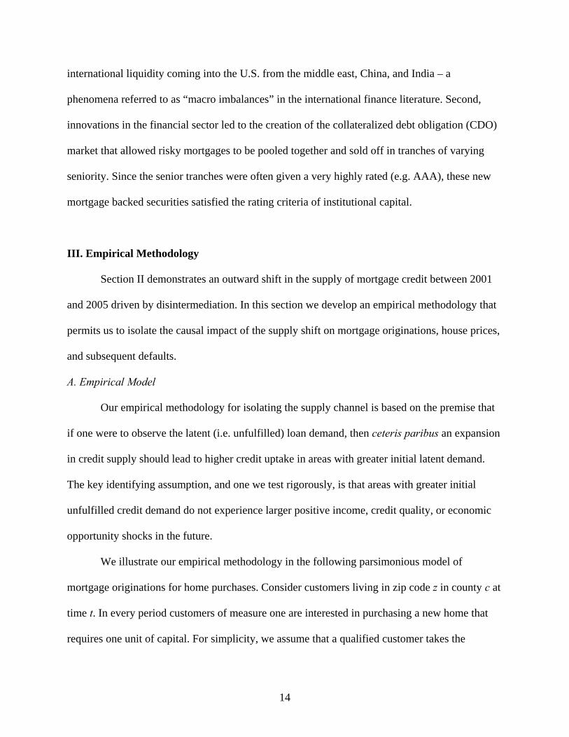
B. Characteristics of High 1996 Latent Demand Zip Codes
As equation (4) demonstrates, initial latent demand (1-fz0) is of primary importance in our
empirical analysis. Table 2 presents the correlation of our main measure of latent demand in a
zip code, the fraction of mortgage applications denied in 1996, with other variables. This
measure is strongly correlated with alternative measures of high latent demand/high credit risk,
such as the fraction of subprime borrowers, the fraction of loans backed by FHA, or the fraction
of housing units rented. It is also strongly correlated with poverty and unemployment, and
negatively correlated with household income measures.
The bottom panel of Table 2 demonstrates that measures of future growth in economic
opportunities are negatively correlated with the fraction of 1996 mortgage applications denied.
As mentioned above, the critical identifying assumption of our empirical methodology is that
areas with high initial latent demand do not experience subsequent increases in income, credit
quality, or economic opportunity. The correlations in Table 2 strongly support the identifying
assumption, given that observable measures of future growth in economic opportunity are in fact
negatively correlated with our primary measure of high 1996 latent demand. This also suggests
that our estimated is an under-estimate of the true coefficient on supply shock β.

19
IV. Credit Expansion, Mortgage Debt, Housing Prices, and Defaults
In this section, we implement the empirical methodology discussed above. Our goal is to
estimate the causal effect of mortgage credit expansion (due to disintermediation) on growth in
mortgage debt, house prices, and mortgage defaults.
A. Credit Expansion to High 1996 Latent Demand Zip Codes
We first demonstrate that high 1996 latent demand zip codes experience a relative
increase in credit supply to riskier borrowers from 2001 to 2005. In Figures 4 through 7, we plot
coefficient estimates from a year-by-year set of county fixed effects regressions of the following
general specification:
, β , , (5)
1997, 1998, … , 2007
In other words, for each year t from 1997 to 2007, we estimate a first-difference county fixed
effects specification relating the change in outcome y for zip code z in county c from year 1996
to year t to our primary measure of high 1996 latent demand, which is the fraction of 1996
mortgage applications denied in the zip code. We plot the coefficient estimates of β for each
year t, along with the corresponding 95% confidence interval. The plotted coefficient estimates
represent the differential effect on the change in outcome y from 1996 to t for high latent demand
zip codes, after controlling for county fixed effects (αc). This methodology allows us to show the
differential effect of mortgage credit expansion on high latent demand zip codes throughout our
sample period, instead of taking a particular stand on exactly the time period over which
expansion occurs. The inclusion of county fixed effects in the first-differenced specification also
takes out all possible shocks affecting the outcome of interest at the county level.

20
Figure 4 examines the differential pattern of denial rates, debt to income ratios, and
disintermediation for high 1996 latent demand zip codes. There is a dramatic differential
decrease in denial rates for high 1996 latent demand zip codes beginning in 2001 and lasting
through 2006. The coefficient estimate for 2004 implies that a one standard deviation increase in
1996 latent demand (0.08) leads to a reduction in the denial rate of 2 percentage points from
1996 to 2004, which is a one-third standard deviation of the left hand side variable. Figure 4B
shows a corresponding increase in the average debt to income ratio of high 1996 latent demand
zip codes. Beginning in 2002, there is a sharp relative increase in the mortgage debt to income
ratio of high 1996 latent demand zip codes. The coefficient estimate for 2005 implies that a one
standard deviation increase in 1996 latent demand leads to a one-third standard deviation
increase in mortgage debt to income ratios from 1998 to 2005.
The reduction in denial rates and increases in mortgage debt to income ratios for high
1996 latent demand zip codes demonstrates a strong shift in the supply of mortgage credit to a
riskier consumer base from 2001 to 2005. Figure 4C shows the source of this credit expansion.
Beginning in 2001, there is a sharp relative rise in disintermediation for high 1996 latent demand
zip codes. The coefficient estimate for 2006 implies that a one standard deviation increase in
1996 latent demand leads to a 2.4 percentage point increase in the fraction of mortgages
disintermediated from 1996 to 2006, which is more than a one-third standard deviation of the left
hand side variable8.
B. The Effect of Credit Expansion on Mortgage Debt and Housing Prices
Figure 4 demonstrates that zip codes for which there is a high fraction of mortgage
applications denied in 1996 experience a large relative increase originators’ willingness to supply
8 There is a “bump” in Figure 4C prior to 2001. However, since the aggregate level of disintermediation does not increase during the pre-2001 period (Figure 3), this bump is unlikely to have much of an effect in the aggregate.

21
credit from 2001 to 2005. This trend appears to be driven in large part due to an increase in the
disintermediation of mortgages and a consequent increase in the risk tolerance of originators. In
this section, we examine the differential effect of the increase in mortgage supply on mortgage
debt and housing prices in high 1996 latent demand zip codes.
Figure 5A plots coefficient estimates of the differential growth in the number of accepted
mortgages for home purchase for high 1996 latent demand zip codes. From 2002 to 2005, the
coefficient estimate on high 1996 latent demand increases by 300%. The coefficient estimate for
2005 implies that a one standard deviation increase in 1996 latent demand (0.08) leads to a
relative increase in the growth rate of accepted mortgage applications from 1996 to 2005 of 24%,
which is a one-half standard deviation of the left hand side variable. There is a slight increase
from 1998 to 2000, but this increase is less than half the increase from 2002 to 2005. The
evidence suggests that high 1996 latent demand zip codes experience dramatic growth in the
number of new homeowners from 2002 to 2005 as a result of the expansion in mortgage supply.
Figure 5B examines the relative growth in mortgage debt outstanding of high 1996 latent
demand zip codes. The figure demonstrates that the sensitivity of mortgage debt growth in a zip
code to high 1996 latent demand increases from 1999 through 2007. The coefficient estimate for
2007 implies that a one standard deviation increase in 1996 latent demand leads to a relative
increase in the growth rate of mortgage debt outstanding from 1996 through 2007 of 4
percentage points, which is one-eighth of a standard deviation of the left hand side variable.9
9 The estimates in Figure 5B are relatively imprecise and small in magnitude compared to other estimates of mortgage growth because the Equifax measure of mortgage debt used in the figure does not differentiate mortgage debt for new home purchase versus mortgage debt obtained through refinancing. This is important because high 1996 latent demand zip codes do not refinance as aggressively in response to declining interest rates as low 1996 latent demand zip codes (something we confirm in the HMDA data that separates originations for refinancing versus home purchase). Interest rates declined sharply from 2001 to 2003, and so there was a relative decrease in mortgage debt due to refinancing for high 1996 latent demand zip codes from 2001 to 2003 even though there was a strong relative increase in mortgage debt for new home purchase for high latent demand zip codes over this time period.

22
Figure 5C shows a sharp relative increase from 2002 to 2006 in the volume of home
purchase loan originations for high 1996 latent demand zip codes. The coefficient estimate for
2006 implies that a one standard deviation change in 1996 latent demand leads to a relative
increase in the growth rate of originated mortgage amounts for home purchase of 28%, which is
one-half standard deviation of the left hand side variable. As in the number of mortgage
applications, there is a relative increase in the growth rate for high 1996 latent demand zip codes
from 1998 to 2000, but the increase from 2002 to 2006 is significantly larger.
Figure 6 demonstrates the effect of increased supply on house price appreciation. Zip
codes with high 1996 latent demand do not experience any higher growth in house prices from
1996 to 1998. However, as credit supply starts to expand disproportionately more in high latent
demand zip codes in 1999 (Figure 5A), they start to experience a relative increase in house price
appreciation. The relative growth in house price appreciation accelerates from 2001 onward. The
coefficient estimate for 2000 implies that a one standard deviation increase in 1996 latent
demand leads to a relative increase in house price appreciation from 1996 to 2000 of 0.8%,
which is less than a one-fifteenth standard deviation in house price appreciation. The coefficient
estimate for 2006 implies that a one standard deviation increase in 1996 latent demand leads to a
relative increase in house price appreciation from 1996 to 2006 of almost 6%, which is one-third
of a standard deviation. It is important to emphasize that the relative increase in housing prices
for high latent demand zip codes occurs despite relative negative income and employment
growth during this time period. The evidence suggests that a significant fraction of relative house
price appreciation from 2001 to 2006 in high 1996 latent demand zip codes is a direct result of
the expansion of mortgage credit supply.

23
As discussed in Section III, the key identifying assumption of our empirical methodology
is that high 1996 latent demand zip codes do not experience future increases in economic
opportunities or income shocks. Table 2 strongly supports this identifying assumption, as it
documents that observable measures of future growth in economic opportunities are negatively
correlated with our measure of high 1996 latent demand. Nonetheless, in Table 3, we control
directly for changes in economic opportunity. More specifically, Table 3 presents coefficient
estimates from the following first difference county fixed effects specification:
, (6)
In (6), X represents a matrix of control variables for economic opportunities including income
growth, wage growth, establishment growth, and employment growth. We also include zip code
level growth in crime rate as measured by the CAP Index crime index to account for variation in
neighborhood safety. We choose the period 2001 to 2005 for the regressions given the evidence
from Figures 4 through 6 that this is the main period over which supply expansion occurs. Minor
variations of this time frame do not affect the results.
Panel A of Table 3 presents the estimates. The coefficient estimate in column 1 implies
that a one standard deviation change in 1996 latent demand leads to a 17% higher growth rate in
originated mortgage amounts for home purchase from 2001 to 2005, which is a one-third
standard deviation of the left hand side variable. The coefficient estimate in column 2 implies
that a one standard deviation change in 1996 latent demand leads to a 3% higher growth rate in
mortgage debt outstanding, which is a one-eighth standard deviation of the left hand side
variable. Finally, the coefficient estimate in column 3 implies that a one standard deviation
change in 1996 latent demand leads to a 3% higher growth rate in house prices, which is a one-
eighth standard deviation of the left hand side variable. The results in Table 3 suggest that
magnitudes are similar after controlling for changes in economic opportunities.

24
In Panel B of Table 3, we examine the differential effect of credit expansion on mortgage
debt and house prices using a more direct measure of relative supply shifts. More specifically,
Panel B presents coefficient estimates from the following specification:
(7)
In other words, we estimate a first difference county fixed effects specification relating the
change in outcome y for zip code z in county c from 2001 to 2005 to the change in denial rates
from 2001 to 2005. We utilize the change in denial rates over this time period to measure the
change in the willingness of lenders to supply mortgage credit to a given zip code. The estimates
in Panel B are largely consistent with the estimates in Panel A. Zip codes that experience a
reduction in denial rates from 2001 to 2005 experience an increase in mortgage amounts
originated for home purchase, mortgage debt outstanding, and house price appreciation.
The evidence in this sub-section demonstrates that increased risk tolerance on behalf of
originators led to a sharp increase in the supply of mortgage credit high 1996 latent demand zip
codes. As a result, these zip codes experienced large increases in originated mortgage amounts
and house prices from 2001 to 2005. Our results suggest that a substantial fraction of relative
house price appreciation and originated mortgage amounts in high 1996 latent demand zip codes
would not have occurred in the absence of the expansion in mortgage credit availability.
C. The Effect of Credit Expansion on Default Rates
The results above suggest that a shift in the supply of mortgage credit caused a significant
increase in mortgage debt outstanding and house prices for zip codes with high 1996 latent
demand for mortgages. In this section, we explore the effect of credit expansion on mortgage
default rates.
Figure 7A replicates the methodology of Figures 4 through 6 with the change in default
rates as the left hand side variable. Figure 7A shows that there is a relative increase in mortgage

25
defaults in 2001 for high 1996 latent demand zip codes. This relative increase during a recession
year is consistent with the results in Table 2 that show that high 1996 latent demand zip codes
are lower income, higher unemployment areas. However, it is important to emphasize that the
2001 increase in defaults is not preceded by a relative decrease in denial rates (Figure 4A) or an
increase in aggregate mortgage debt to income ratios (Figure 4B). In other words, there is less
evidence that the relative increase in default rates for high 1996 latent demand zip codes in 2001
is due to an expansion of credit supply. Instead, it appears to be driven primarily by the
economic slowdown.
Figure 7A also shows a sharp increase in default rates for high 1996 latent demand zip
codes from 2005 to the second quarter of 2007. In contrast to the relative increase in defaults in
2001, this increase is not preceded by or concurrent with a recession. Instead, the increase in
defaults for high 1996 latent demand zip codes is preceded by a decline in denial rates (Figure
4A) and an increase in aggregate mortgage debt to income ratios (Figure 4B). These facts
suggest that the relative increase in default rates from 2005 to 2007 is due to the rapid expansion
in the supply of credit from 2001 to 2005. In terms of magnitudes, a one standard deviation
increase in 1996 latent demand for a zip code leads to a 1 percentage point increase in default
rates from 1996 to 2007, which is one-third standard deviation of the left hand side variable.
In Figure 7B, we examine the differential effect of credit expansion on mortgage default
rates by using a time-varying measure of relative supply shifts. More specifically, Figure 7B
plots coefficient estimates from a year-by-year set of county fixed effects regressions of the
following general specification:
, β , , (8)
2001, 2002, … , 2007

26
In other words, for each year t from 2001 to 2007, we estimate a first difference county fixed
effects specification relating the change in default rates for zip code z in county c from year t-2 to
year t to the change in denial rates from t-5 to t-3. For example, for t = 2007, the specification
estimates whether default rates from 2005 to 2007 are correlated with changes in denial rates
from 2002 to 2004. We utilize the change in denial rates as a measure of the change in the
willingness of lenders to supply mortgage credit to a given zip code.
Figure 7B shows the year-by-year estimates. It demonstrates that the only year in our
sample for which changes in default rates are negatively correlated with lagged changes in denial
rates is 2007. In other words, zip codes that experienced a reduction in denial rates from 2002 to
2004 experience an increase in default rates from 2005 to 2007.
In columns 1 and 2 of Table 4, we examine a reduced form specification relating the
change in default rates from 2005 to 2007 to 1996 latent demand and the change in denial rates
from 2001 to 2005, respectively. The two right hand side variables measure zip codes that
experience a relative increase in the supply of credit from 2001 to 2005; therefore, the coefficient
estimates represent the reduced form effect of credit expansion on default rates. The estimate in
column 1 implies that a one standard deviation increase in 1996 latent demand leads to a 0.52%
increase in default rates from 2005 to 2007, which is a one-fifth standard deviation increase in
the left hand side variable.
In columns 3 through 6 of Table 4, we examine the effect of supply-driven mortgage
growth and house price growth from 2001 to 2005 on the change in default rates from 2005 to
2007. We define supply driven mortgage growth and house price growth as the predicted values
from first stage regressions relating mortgage growth and house price growth from 2001 to 2005
to either the fraction of 1996 mortgage applications denied or the change in denial rates from

27
2001 to 2005. The first stage estimates used to predict supply driven mortgage growth and house
price growth are in columns 1 and 3 of Table 3.
The estimates in columns 3 through 6 of Table 4 demonstrate that supply driven
mortgage growth and house price growth from 2001 to 2005 have a strong effect on the increase
in default rates from 2005 to 2007. The estimate in column 3 implies that a one standard
deviation increase in supply driven mortgage growth from 2001 to 2005 leads to a 1.6 percentage
point increase in default rates, which is more than a one-half standard deviation increase of the
left hand side variable. A one standard deviation increase in supply driven house price
appreciation leads to a 5 percentage point increase in default rates, which is almost a two
standard deviation change in the left hand side variable.
D. Disintermediation and Moral Hazard
The evidence in the section above demonstrates that house price appreciation and debt
growth driven by an increase in the supply of mortgage credit from 2001 to 2005 caused
substantial increases in default rates. The evidence also suggests that investors that entered this
market experienced large losses as a result of the expansion in credit. For example, our estimates
imply that a 10% expansion in mortgage credit from 2001 to 2005 to high 1996 latent demand
zip codes caused a 3 percentage point increase in default rates, which is a doubling of the sample
average. Given that foreclosure recovery rates are typically between 40 and 70% (Pence (2006)),
the increase in default rates represented significant losses for mortgage investors. In addition, the
subprime-prime mortgage spread fell to historical lows during this period, which suggests that
investors were not compensated for the additional ex post risk. These losses beg the question:
Why did investors agree to fund these mortgages?

28
Figure 3 above shows that the sharp rise in mortgage growth coincides with the increase
in disintermediation of mortgages. Moreover, the disintermediation is significantly stronger in
zip codes with high 1996 latent demand for loans (Figure 4C). Models of financial
disintermediation and moral hazard argue that financial intermediaries exerting unobservable
monitoring effort must hold a significant fraction of credit risk to ensure proper incentives
(Holmtrom and Tirole (1997), He and Krishnamurthy (2006)). The findings above suggest that
moral hazard on behalf of loan originators that no longer hold a stake in risky loans is a potential
cause of the increase in default rates.
In Table 5, we present further evidence of originator moral hazard. Column 1 in Panel A
reaffirms the result shown earlier in Figure 4C: High initial latent demand zip codes experience a
larger increase in fraction of loans sold off to investors within a year. Columns 2 through 6 of
Panel A break down the fraction sold by the identity of the party buying the mortgage from the
originating institution. The correlation between high latent demand and disintermediation is
being driven by mortgages sold in private securitizations to unaffiliated investors, and to non-
bank financial firms. In other words, high latent demand zip codes did not experience an increase
in the fraction of mortgages sold to affiliated institutions or banks.
Column 1 of Panel B demonstrates that zip codes experiencing a relative increase in
disintermediation also experience increases in mortgage debt to income ratios, which is
consistent with originators shedding credit risk during the 2001 to 2005 expansion. Columns 2
through 6 show the correlation of the fraction of loans sold in a zip code from 2001 to 2005 by
the type of investor buying the mortgage with subsequent default rates from 2005 to 2007. The
estimates demonstrate that zip codes in which a larger fraction of mortgages are sold in private

29
securitizations and to non-commercial bank financial firms experience relatively larger increases
in default rates from 2005 to 2007.
In contrast, column 2 of Panel B shows that zip codes in which originators sell more
mortgages to affiliated investors do not experience an increase in default rates. Under the
assumption that originators’ incentives are more closely aligned with affiliated versus non-
affiliated investors, these results suggest that undetected moral hazard is a primary cause for the
higher default rates on mortgages sold to non-affiliated investors. In addition, column 5 of Table
5 demonstrates that zip codes in which originators sell more mortgages to other commercial
banks do not experience an increase in default rates. Given that commercial banks have
specialized skill in screening loans, these results suggest that originators only sold bad loans to
unaffiliated investors lacking the skills to judge loan quality. Together with the findings in Panel
A, these findings support the hypothesis that moral hazard on behalf of originators is a main
culprit for the rise in default rates.
A caveat is in order. Unlike the results above that demonstrate a causal effect of mortgage
credit expansion on house price appreciation and subsequent defaults, we view our evidence on
moral hazard as suggestive. In other words, it is more difficult to assert that undetected moral
hazard on behalf of originators caused the spike in mortgage defaults for two reasons. First, there
is the lack of exogenous within-county variation across zip codes in the ability of originators to
sell mortgages. Without such variation, it is difficult to rule out alternative explanations. Second,
we do not have loan-level interest rate data, which makes it difficult to examine whether moral
hazard is priced. Nonetheless, our suggestive findings are supported by both academic and
anecdotal evidence. Keys, Mukherjee, Seru and Vig (2008) exploit cutoffs in FICO scores
required for securitization of mortgages to show that securitization causes an increase in default

30
rates, which they interpret as evidence of bank moral hazard. They show that interest rate
differentials between mortgages above and below the cutoffs are similar. In addition, as
mentioned above, interest rates on subprime mortgage declined to historical lows during this
time period, which suggests that investors did not price increased moral hazard concerns. Finally,
anecdotal evidence on moral hazard of originators is plentiful (see Zuckerman, WSJ, January
15th, 2008; Ng and Mollenkamp, WSJ, January 14th, 2008; and Pleven and Craig, WSJ, January
17th, 2008).
E. Robustness
In this section, we present two sets of robustness tests to ensure that the estimates
presented above reflect our credit expansion interpretation. The specifications reported in Table
6 examine non-home consumer debt, which includes credit card, auto, student, and consumer
loans. Given that our supply interpretation is unique to the expansion in mortgage debt
availability in high latent demand zip codes, we do not expect to find the same pattern in debt
growth and defaults for non-home consumer debt. As Table 6 demonstrates, high 1996 latent
demand zip codes experience a relative reduction in non-home debt from 2001 to 2005. This
result also mitigates the concern that high 1996 latent demand zip codes are experiencing
increases in economic opportunity over this time period, and it suggests that households may
respond to mortgage credit expansion by reducing other consumer debt. Columns 3 and 4
demonstrate that high 1996 latent demand zip codes do not experience any differential increase
in default rates on non-home debt, which helps rule out alternative stories for our results.
In Table 7, we examine alternative measures of high 1996 latent demand. As we
discussed in Section III, our empirical methodology relies on variation across zip codes in the
initial fraction of borrowers that cannot obtain mortgages due to excessive credit risk. In Table 7,

31
we examine the fraction of loans backed by the Federal Housing Authority in a zip code in 1996,
the fraction of subprime borrowers in the zip code in 1996, and the fraction of housing units
occupied by renters in a zip code in 2000 as alternative measures of initial high latent demand.
As the estimates in Table 7 demonstrate, our core results are robust to these alternative measures
of high latent demand. The magnitudes of the second stage coefficients are larger for the FHA
and subprime shares, and slightly smaller for the fraction of units rented.
V. Concluding Remarks: What are the Macro-Economic Magnitudes of the Supply Shift?
The process of disintermediation in the mortgage industry led to a sharp shift in the
supply of mortgage credit from 2001 to 2005. The expansion in supply was targeted at subprime
customers who were traditionally marginal borrowers unable to access the mortgage market. The
shift in mortgage supply consequently led to a rapid rise in the risk profile of borrowers, and a
surge in supply-induced house price and mortgage credit growth. These changes caused a
subsequent spike in default rates, which have in turn depressed the housing market and caused
financial market turmoil.
The main contribution of our work is to empirically isolate the mechanism, magnitude,
and consequences of the historic shift in mortgage supply. Given that we have identified the
expansion in credit and increase in house price due to the shift in the supply of credit, we can use
our microeconomic estimates to answer an important macroeconomic counter-factual: How
would mortgage lending and house prices have evolved if the shift in supply in the mortgage
industry had not occurred?
To answer this question, we sort zip codes by 1996 denial rates and categorize them into
20 equal bins with 5% of zip codes in each bin. Let i index each bin, and denote by di the median

32
denial rate inside a 5% bin. Given a coefficient of 2.11 (Table 3, column 1) for the marginal
effect of initial denial rate on mortgage growth from 2001 to 2005, the incremental supply-
induced loan origination in bin i is equal to 2.11*Li,2001*(di – d1), where Li,2001 is aggregate loan
origination in bin i in 2001. The total supply-induced loan origination in 2005 is thus equal to:
2.11 L , d – d
The calculation above assumes that our estimated effect of 2.12 is linear over the entire data
distribution. We estimate a non-parametric plot of this coefficient and find that linearity is a
reasonable approximation.
A similar calculation for calculating the average increase in house prices due to supply-
shift between 2001 and 2005 can be written as:
0.34 w , d – d
where 0.34 is the house price growth coefficient from column 3 of Table 3, and w , is the
weight of bin i according to the share of loan originations belonging to that zip code.10 Solving
the above expressions in our data gives us $83 billion of additional home purchase loan
originations in 2005 due to supply shift, or 15% of total home purchase originations in 200511.
Similarly we get a 4.3% increase in house prices between 2001 and 2005 due to supply shift, or
almost 10% of aggregate house price appreciation in the US between 2001 and 2005.
It is important to emphasize that the calculations described above are an underestimate of
the true impact of supply shift for two reasons. First, changes in borrower credit quality are
10 Alternatively we could have given each bin an equal weight of 1/20, which essentially gives the same result. Also our exact calculation is slightly different in that we convert log changes to percentage changes by taking their exponent and subtracting 1. 11 To remain consistent with the calculation, we only include the zip codes that are part of our study in computing the total home purchase originations.

33
negatively correlated with initial latent demand for mortgages which biases downward our
regression estimates (as described in Section III). Second, since our empirical methodology is
based on a difference-in-differences estimator, we can only estimate the relative impact of the
shift in supply. In other words, we estimate the differential effect of the supply shift on high
1996 latent demand zip codes relative to low 1996 latent demand zip codes. Consequently, our
calculation above disregards any level impact of the supply shift which impact all zip codes.
There is evidence to suggest that this may be a significant omission. For example, even zip codes
with low denial rates in 1996 took advantage of the lower lending rates by taking out home
equity loans and refinancing in large amounts. The effect of the supply shift on the intensive
margin of higher credit quality home-owners is material for future research.

34
References
Brunnermeier, Markus and Christian Julliard, 2007. “Money Illusion and Housing Frenzies,” Review of Financial Studies, forthcoming. Case, Karl, and Robert Shiller, 1989. “The Efficiency of the Market for Single-Family Homes,” American Economic Review 79: 125-137. Chomsisengphet, Souphala and Anthony Pennington-Cross, 2006. “The Evolution of the Subprime Mortgage Market,” Federal Reserve Bank of St. Louis Review 88: 31-56. Demyanyk and Van Hemert, 2007, “Understanding the Subprime Mortgage Crisis”, Working Paper, New York University. Diamond, D., 1991, “Monitoring and reputation: The choice between bank loans and privately placed debt,” Journal of Political Economy, 99, 689-721. Doms, Mark, Fred Furlong, and John Krainer, 2007. “Subprime Mortgage Delinquency Rates,” Federal Reserve Bank of San Francisco Working Paper. Gabriel, Stuart and Stuart Rosenthal, 2007, “Secondary Markets, Risk, and Access to Credit: Evidence from the Mortgage Market,” Working Paper, Syracuse University. Garmaise, Mark and Tobias Moskowitz, “Bank Mergers and Crime: The Real and Social Effects of Credit Market Competition,” Journal of Finance 61: 495-538. Genesove, David, and Christopher Mayer, 1997. “Equity and Time to Sale in the Real Estate Market,” American Economic Review, 87: 255-269. --, 2001, “Loss Aversion and Seller Behavior: Evidence from the Housing Market,” Quarterly Journal of Economics, 1233-1260. Glaeser, Edward and Joseph Gyourko, 2005, “Urban Decline and Durable Housing,” Journal of Political Economy 113: 345-375. He, Zhiguo, and Arvind Krishnamurthy, 2006. “Intermediation, Capital Mobility, and Asset Prices,” Working Paper, Northwestern University. Himmelberg, Charles, Christopher Mayer, and Todd Sinai, 2005, “Assessing High House Prices: Bubbles, Fundamentals, and Misperceptions,” Journal of Economic Perspectives 19: 67-92. Holmstrom, B. and J. Tirole, 1997, “Financial intermediation, loanable funds, and the real sector,” Quarterly Journal of Economics, 112, 663-691. Hurst, Erik and Frank Stafford, 2004, “Home is Where the Equity Is: Mortgage Refinancing and Household Consumption,” Journal of Money, Credit, and Banking 36: 985-1014.

35
Keys, Benjamin, Tanmoy Mukherjee, Amit Seru and Vikrant Vig 2008, “Securitization and Screening: Evidence From Subprime Mortgage Backed Securities”, working paper. Pence, Karen, 2006, “Foreclosing on Opportunity: State Laws and Mortgage Credit,” Review of Economics and Statistics, vol. 88 (February 2006), pp. 177-182 Poterba, James, 1984. “Tax Subsidies to Owner-Occupied Housing: An Asset-Market Approach,” Quarterly Journal of Economics 99: 729-752. Reinhart, Carmen and Kenneth Rogoff, 2008, “Is the 2007 U.S. Sub-Prime Financial Crisis So Different? An International Historical Comparison”, Mimeo, Harvard University. Stein, Jeremy, 1995. “Prices and Trading Volume in the Housing Market: A Model with Down-Payment Effects,” Quarterly Journal of Economics 110: 379-406. Stiglitz, Joseph and Andrew Weiss, 1981. “Credit Rationing in Markets with Imperfect Information,” American Economic Review 71: 393-410.
0.5
1
1.5
2
2.5
3
1992 1993 1994 1995 1996 1997 1998 1999 2000 2001 2002 2003 2004 2005 2006 2007
Figure 1AHousing Prices, Indexed to 1996
This figure presents the house price index for the U.S. from 1992 to 2007, indexed to 1996. The house price index is constructed from the equal-weighted average of the 2,920 zip codes in our final sample. Data are from Fiserv Case Shiller Weiss
0
0.5
1
1.5
2
2.5
3
3.5
1992 1993 1994 1995 1996 1997 1998 1999 2000 2001 2002 2003 2004 2005 2006 2007
Figure 1BMortgage and non-Mortgage Debt Outstanding, Indexed to 1996
Mortgage debt outstanding non Mortgage debt outstanding
This figure presents total mortgage and non-mortgage consumer debt outstanding for the U.S. from 1992 to 2007, indexed to 1996. Total non-mortgage consumer debt includes student loans, auto loans, consumer loans, and outstanding credit card balances. Data are from Equifax Predictive Services.
Mortgage debt outstanding non-Mortgage debt outstanding
0.8
1
1.2
1.4
1.6
1.8
2
2.2
1996 1997 1998 1999 2000 2001 2002 2003 2004 2005 2006
Figure 1CAccepted Mortgage Applications for Home Purchase, Indexed to 1996
This figure presents the number of accepted mortgage applications for home purchase from 1996 to 2006, indexed to 1996. Data are from HMDA.
0.6
0.7
0.8
0.9
1
1.1
1.2
1.3
1.4
1.5
1.6
1992 1993 1994 1995 1996 1997 1998 1999 2000 2001 2002 2003 2004 2005 2006 2007
Figure 1DDefault Rates for Mortgage and non-Mortgage Debt , Indexed to 1996
Mortgage debt default rates non-Mortgage debt default rates
This figure presents the default rate for consumer debt outstanding for the U.S. from 1992 to 2007, indexed to 1996. The total non-mortgage default rate iscalculated using non-mortgage debt which includes student loans, auto loans, consumer loans, and outstanding credit card balances. Data are from Equifax Predictive Services.

0
0.2
0.4
0.6
0.8
1
1.2
1.4
1996 1997 1998 1999 2000 2001 2002 2003 2004 2005 2006
Figure 2ADebt to Income Ratios for Accepted Mortgage Applications, Relative to 1996
Debt to Income of Accepted Applications--Median Debt to Income of Accepted Applications--75th Percentile
This figure presents the mortgage debt to income ratios of accepted mortgage applications at the median, 75th, and 90th percentiles from 1996 to 2006. The 1996 level is substracted from each series. Data are from HMDA.
p pp p ppDebt to Income of Accepted Applications--90th Percentile
0
0.02
0.04
0.06
0.08
0.1
0.12
0.14
0.16
1998 1999* 2000* 2001 2002 2003* 2004 2005
Figure 2BOriginated Mortgage Debt for Home Purchase to Income Ratios, Relative to 1996
This figure presents the average originated mortgage debt to aggregate income ratio across zip codes from 1998 to 2005. The 1998 level is substractedfrom the series. Originated mortgage debt is from HMDA and aggregate income is from the IRS. * indicates data missing for the year in question.

0.45
0.5
0.55
0.6
Figure 3Fraction of Mortgages Sold to Non-Mortgage Agency Institutions
This figure presents the fraction of originated mortgages that are sold to non-mortgage agency institutions within one year of origination. Non-mortgage agency institutions include all third parties except for Fannie Mae, Freddie Mac, Ginnie Mae, and Farmer Mac. Data are from HMDA.
0.2
0.25
0.3
0.35
0.4
1996 1997 1998 1999 2000 2001 2002 2003 2004 2005 2006

-0.35
-0.3
-0.25
-0.2
-0.15
-0.1
-0.05
0
0.05
0.1
1996 1997 1998 1999 2000 2001 2002 2003 2004 2005 2006
Figure 4AMortgage Denial Rates For High 1996 Denial Zip Codes
This figure plots the estimated coefficients of β and 95% confidence intervals for each year for the following first difference county fixed effects specifications:
,1996 ,1996* 1997,1998,...,2007zct zc c t zc zctDenied Denied HighLatentDemand for tα β ε− = + + =
0
0.1
0.2
0.3
0.4
0.5
0.6
0.7
0.8
1998 1999* 2000* 2001 2002 2003* 2004 2005
Figure 4BOriginated Mortgage Debt to Income Ratio For High 1996 Denial Zip Codes
This figure plots the estimated coefficients of β and 95% confidence intervals for each year for the following first difference county fixed effects specifications:
* indicates data missing for the year in question.,1996 ,19962 2 * 1997,1998,...,2007zct zc c t zc zctD I D I HighLatentDemand for tα β ε− = + + =

Figure 4CFigure 4CDisintermediation For High 1996 Denial Zip Codes
This figure plots the estimated coefficients of β and 95% confidence intervals for each year for the following first difference county fixed effects specifications:
Disintermediated loans are loans sold to any third party except for Fannie Mae Freddie Mac Ginnie Mae and Farmer Mac within 1 year of origination
,1996 ,1996* 1997,1998,...,2007zct zc c t zc zctSold Sold HighLatentDemand for tα β ε− = + + =
0 3
0.35
Disintermediated loans are loans sold to any third party except for Fannie Mae, Freddie Mac, Ginnie Mae, and Farmer Mac within 1 year of origination.
0.25
0.3
0.15
0.2
0.1
0.15
0
0.05
-0.05
1996 1997 1998 1999 2000 2001 2002 2003 2004 2005 2006

-0.5
0
0.5
1
1.5
2
2.5
3
3.5
1996 1997 1998 1999 2000 2001 2002 2003 2004 2005 2006
Figure 5ANumber of Originated Mortgages for Home Purchase For High 1996 Denial Zip Codes
This figure plots the estimated coefficients of β and 95% confidence intervals for each year for the following first difference county fixed effects specifications:
,1996 ,1996( ) ( ) * 1997,1998,...,2007zct zc c t zc zctLn Orig Ln Orig HighLatentDemand for tα β ε− = + + =
-0.2
-0.1
0
0.1
0.2
0.3
0.4
0.5
0.6
0.7
0.8
1996 1997 1998 1999 2000 2001 2002 2003 2004 2005 2006 2007
Figure 5BOutstanding Mortgage Debt For High 1996 Denial Zip Codes
This figure plots the estimated coefficients of β and 95% confidence intervals for each year for the following first difference county fixed effects specifications:
,1996 ,1996( ) ( ) * 1997,1998,...,2007zct zc c t zc zctLn MortgageDebt Ln MortgageDebt HighLatentDemand for tα β ε− = + + =

2.5
3
3.5
4
Figure 5CAmount of Originated Mortgages for Home Purchase For High 1996 Denial Zip Codes
This figure plots the estimated coefficients of β and 95% confidence intervals for each year for the following first difference county fixed effects specifications:
,1996 ,1996( ) ( ) * 1997,1998,...,2007zct zc c t zc zctLn Amt Ln Amt HighLatentDemand for tα β ε− = + + =
-0.5
0
0.5
1
1.5
2
1996 1997 1998 1999 2000 2001 2002 2003 2004 2005 2006

0.5
0.6
0.7
0.8
Figure 6Relative House Price Appreciation For High 1996 Denial Zip Codes
This figure plots the estimated coefficients of β and 95% confidence intervals for each year for the following first difference county fixed effects specifications:
,1996 ,1996( ) ( ) * 1997,1998,...,2007zct zc c t zc zctLn HP Ln HP HighLatentDemand for tα β ε− = + + =
-0.1
0
0.1
0.2
0.3
0.4
1996 1997 1998 1999 2000 2001 2002 2003 2004 2005 2006 2007

0
0.02
0.04
0.06
0.08
0.1
0.12
0.14
1996 1997 1998 1999 2000 2001 2002 2003 2004 2005 2006 2007
Figure 7AMortgage Default Rates for High 1996 Denial Zip Codes
This figure plots the estimated coefficients of β and 95% confidence intervals for each year for the following first difference county fixed effects specifications:
,1996 ,1996* 1997,1998,...,2007zct zc c t zc zctDefRate DefRate HighLatentDemand for tα β ε− = + + =
-0.02
-0.15
-0.1
-0.05
-1E-16
0.05
0.1
2001 2002 2003 2004 2005 2006 2007
Figure 7BMortgage Default Rates by Lagged Change in Denial Rates
This figure plots the estimated coefficients of β and 95% confidence intervals for each year for the following first difference county fixed effects specifications:
For example, for t = 2007, the coefficient estimate shows how default rates change from 2005 to 2007 for zip codes experiencing a change in denial rates from 2002 to 2004.
, 2 , 3 , 5*( ) 2001,...,2007zct zc t c t zc t zc t zctDefRate DefRate Denied Denied for tα β ε− − −− = + − + =

Table 1 Summary Statistics
This table presents summary statistics for the 2,920 zip codes in our sample. Mean SD 10th 50th 90th Equifax Data Mortgage debt as fraction of total debt, 1996 0.741 0.106 0.600 0.761 0.854 Home equity debt as fraction of total debt, 1996 0.044 0.028 0.018 0.037 0.075 Non-home debt as fraction of total debt, 1996 0.215 0.085 0.121 0.201 0.330 Mortgage debt annualized growth, 1996 to 2001 0.069 0.042 0.023 0.068 0.115 Non-home debt annualized growth, 1996 to 2001 0.061 0.042 0.019 0.061 0.103 Mortgage debt annualized growth, 2001 to 2005 0.102 0.046 0.054 0.103 0.149 Non-home debt annualized growth, 2001 to 2005 0.046 0.046 -0.007 0.047 0.098 Mortgage default rate, 1996 0.030 0.024 0.005 0.024 0.060 Non-home default rate, 1996 0.069 0.035 0.029 0.063 0.114 Mortgage default rate change, 1996 to 2005 -0.003 0.028 -0.032 -0.004 0.025 Non-home default rate change, 1996 to 2005 -0.008 0.030 -0.041 -0.007 0.024 Mortgage default rate change, 2005 to 2007 0.017 0.027 -0.009 0.014 0.051 Non-home default rate change, 2005 to 2007 0.009 0.024 -0.016 0.009 0.034 Sub-prime consumer fraction (under 659) 0.288 0.112 0.156 0.270 0.447 Fiserve Case Shiller Weiss Data Home price annualized growth, 1996 to 2001 0.073 0.023 0.041 0.075 0.102 Home price annualized growth, 2001 to 2005 0.113 0.044 0.039 0.117 0.166 HMDA Data Mortgages for home purchase annualized growth, 1996 to 2001 0.095 0.046 0.039 0.097 0.152 Mortgages for home purchase annualized growth, 2001 to 2005 0.134 0.078 0.048 0.136 0.220 Fraction of applications denied, 1996 0.219 0.079 0.122 0.211 0.329 Fraction of mortgages sold to non-agency investors, 2001 0.277 0.074 0.184 0.275 0.374 Change in fraction sold to non-agency investors, 2001 to 2005 0.263 0.057 0.191 0.262 0.334 Fraction of mortgages backed by FHA, 1996 0.129 0.111 0.014 0.097 0.283 Decennial Census, IRS, and Census Statistics of U.S. Business Median household income, thousands, 2000 55.7 20.0 33.4 52.5 81.8 Fraction non-white, 2000 0.202 0.197 0.028 0.132 0.496 Fraction with education less than high school, 2000 0.166 0.117 0.051 0.135 0.320 Fraction unemployed, 2000 0.051 0.032 0.023 0.042 0.091 Fraction of housing units rented, 2000 0.300 0.160 0.105 0.277 0.529 Income growth (from IRS), 2001 to 2005 0.127 0.094 0.033 0.114 0.241 Wage growth (from Business Conditions), 2001 to 2004 0.072 0.121 -0.050 0.072 0.196 Employment growth, 2001 to 2004 0.025 0.192 -0.172 0.017 0.217 Establishment growth, 2001 to 2004 0.057 0.100 -0.039 0.046 0.170 Crime index growth, 2001 to 2005 0.024 0.050 -0.027 0.016 0.087
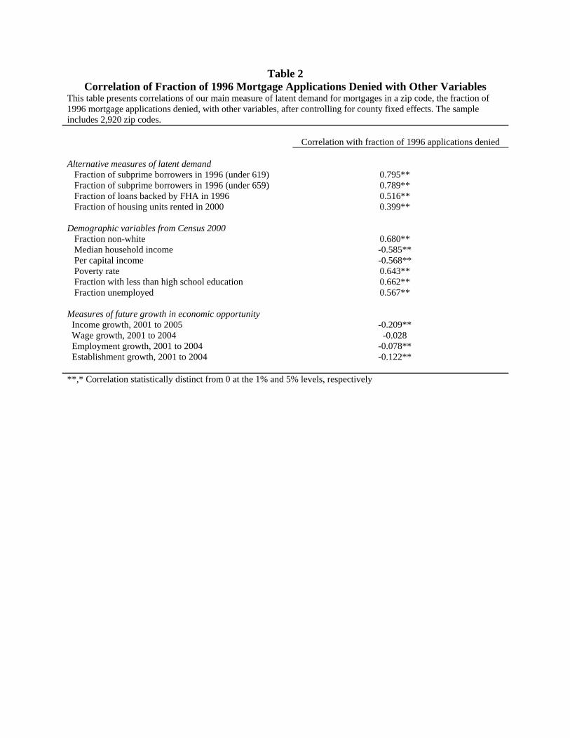
Table 2 Correlation of Fraction of 1996 Mortgage Applications Denied with Other Variables
This table presents correlations of our main measure of latent demand for mortgages in a zip code, the fraction of 1996 mortgage applications denied, with other variables, after controlling for county fixed effects. The sample includes 2,920 zip codes. Correlation with fraction of 1996 applications denied Alternative measures of latent demand Fraction of subprime borrowers in 1996 (under 619) 0.795** Fraction of subprime borrowers in 1996 (under 659) 0.789** Fraction of loans backed by FHA in 1996 0.516** Fraction of housing units rented in 2000 0.399** Demographic variables from Census 2000 Fraction non-white 0.680** Median household income -0.585** Per capital income -0.568** Poverty rate 0.643** Fraction with less than high school education 0.662** Fraction unemployed 0.567** Measures of future growth in economic opportunity Income growth, 2001 to 2005 -0.209** Wage growth, 2001 to 2004 -0.028 Employment growth, 2001 to 2004 -0.078** Establishment growth, 2001 to 2004 -0.122** **,* Correlation statistically distinct from 0 at the 1% and 5% levels, respectively

Table 3 The Effect of Mortgage Credit Expansion on Mortgage Amounts and House Prices
Columns 1 and 2 of Panel A present estimates of the effect of high 1996 latent demand in a zip code on growth in originated mortgage amount for home purchase and growth in mortgage debt outstanding from 2001 to 2005, respectively. Column 3 presents estimates of the effect of high 1996 latent demand in a zip code on growth in house prices from 2001 to 2005. Panel B examines how outcomes vary with an alternative measure of zip codes receiving a relative increase in supply: the change in denial rates from 2001 to 2005. All specifications include county fixed effects. Panel A: Fraction of 1996 applications denied (1) (2) (3) Originated mortgage
amount for home purchase growth
2001 to 2005
Mortgage debt outstanding growth
2001 to 2005
House price growth 2001 to 2005
Fraction of 1996 applications denied 2.109**
(0.115) 0.444** (0.064)
0.339** (0.016)
Income growth, 2001 to 2005 0.103
(0.083) 0.500** (0.046)
-0.031** (0.011)
Wage growth, 2001 to 2004 -0.036 (0.057)
0.044 (0.031)
-0.004 (0.008)
Establishment growth, 2001 to 2004 0.008 (0.042)
-0.015 (0.023)
0.009 (0.006)
Employment growth, 2001 to 2004 0.011 (0.090)
0.669** (0.050)
-0.032** (0.012)
Crime growth, 2001 to 2005
-0.050 (0.162)
0.408** (0.090)
-0.079** (0.022)
N 2897 2897 2897 R2 0.41 0.30 0.96 Panel B: Change in denial rates from 2001 to 2005 (1) (2) (3) Originated mortgage
amount for home purchase growth
2001 to 2005
Mortgage debt outstanding growth
2001 to 2005
House price growth 2001 to 2005
Change in denial rates, 2001 to 2005 -3.868**
(0.198) -0.477** (0.111)
-0.557** (0.027)
Income growth, 2001 to 2005 -0.068
(0.081) 0.448** (0.045)
-0.062** (0.011)
Wage growth, 2001 to 2004 -0.065 (0.056)
0.038 (0.031)
-0.009 (0.008)
Establishment growth, 2001 to 2004 0.015 (0.041)
-0.016 (0.023)
0.010** (0.006)
Employment growth, 2001 to 2004 -0.079 (0.089)
0.650** (0.050)
-0.046** (0.012)
Crime growth, 2001 to 2005
-0.183 (0.159)
0.335** (0.089)
-0.109** 0.022
N 2897 2897 2897 R2 0.42 0.29 0.96 **,* Coefficient estimate statistically distinct from 0 at the 1% and 5% levels, respectively

Table 4 The Effect of Mortgage Credit Expansion on Mortgage Default Rates
This table presents estimates of how the shift in mortgage supply from 2001 to 2005 affects default rates from 2005 to 2007. Columns 1 and 2 report estimates from the reduced form relating the increase in defaults from 2005 to 2007 to measures of zip codes experiencing relative supply increases from 2001 to 2005. Columns 3 through 6 relate the increase in default rates from 2005 to 2007 to measures of supply driven house price growth and mortgage origination growth, which are obtained from a first stage that relates these variables to two different supply shifters: the fraction of denied applications in 1996 and the change in denial rates from 2001 to 2005. The first stage estimates are in Table 3. All specifications include county fixed effects. (1) (2) (3) (4) (5) (6) Change in mortgage default rates from 2005 to 2007 Fraction of 1996 applications denied
0.066** (0.008)
Change in denial rates, 2001 to 2005
-0.092** (0.014)
Supply driven originated mortgage amount for home purchase growth, 2001 to 2005
0.031** (0.004)
0.024** (0.004)
Supply driven house price growth, 2001 to 2005
0.194** (0.024)
0.165** (0.025)
Income growth, 2001 to 2005 -0.033**
(0.006) -0.040** (0.006)
-0.036** (0.006)
-0.027** (0.006)
-0.038** (0.006)
-0.030** (0.006)
Wage growth, 2001 to 2004 0.003 (0.004)
0.003 (0.004)
0.005 (0.004)
0.004 (0.004)
0.004 (0.004)
0.004 (0.004)
Establishment growth, 2001 to 2004 -0.001 (0.003)
-0.001 (0.003)
-0.001 (0.003)
-0.003 (0.003)
-0.002 (0.003)
-0.003 (0.003)
Employment growth, 2001 to 2004 0.011 (0.006)
0.008 (0.006)
0.010 (0.006)
0.017** (0.006)
0.010 (0.006)
0.015* (0.006)
Crime growth, 2001 to 2005
0.004 (0.011)
-0.004 (0.011)
0.005 (0.012)
0.019 (0.012)
0.000 (0.011)
0.014 (0.012)
Supply shifter? Reduced form Reduced form 1996 Denied
applications 1996 Denied applications
Change in denial rates, 2001 to 2005
Change in denial rates, 2001 to 2005
N 2897 2897 2897 2897 2897 2897 R2 0.20 0.19 0.11 0.16 0.16 0.18 **,* Coefficient estimate statistically distinct from 0 at the 1% and 5% levels, respectively

Table 5 Evidence of a Disintermediation Channel
Panel A presents coefficient estimates relating the change in the fraction of originated mortgages sold in a zip code to latent demand as of 1996. Column 1 of Panel B relates the change in median debt to income ratios of accepted applications from 2001 to 2005 to the change in the fraction of loans sold to investors. Columns 2 through 5 of Panel B presents estimates relating default rates from 2005 to 2007 to the fraction of loans sold by originators to investors from 2001 to 2005. All specifications include county fixed effects and control variables for income, wage, employment, establishment, and crime growth.
Panel A: High latent demand zip codes and mortgage sales (1) (2) (3) (4) (5) Change in fraction
sold to all investors, 2001 to
2005
Change in fraction sold to affiliates,
2001 to 2005
Change in fraction sold in private securitizations, 2001 to 2005
Change in fraction sold to banks, 2001
to 2005
Change in fraction sold to non-bank
financial firms, 2001 to 2005
Fraction of 1996 applications denied 0.161**
(0.014) -0.072** (0.008)
0.177** (0.006)
0.004 (0.004)
0.125** (0.006)
N 2897 2897 2897 2897 2897 R2 0.47 0.54 0.63 0.45 0.58
Panel B: Mortgage sales and changes in default rates (1) (2) (3) (4) (5) (6) Change in Debt
to Income Ratio 2001 to 2005
Change in mortgage default rates from 2005 to 2007
Change in fraction sold to all investors, 2001 to 2005 0.314**
(0.056) 0.042** (0.011)
Change in fraction sold to affiliates, 2001 to 2005
-0.105** (0.019)
Change in fraction sold in private securitizations, 2001 to 2005
0.147** (0.023)
Change in fraction sold to banks , 2001 to 2005
-0.023 (0.036)
Change in fraction sold to non-bank financial firms , 2001 to 2005
0.136** (0.023)
N 2919 2897 2897 2897 2897 2897 R2 0.77 0.18 0.18 0.19 0.17 0.19 **,* Coefficient estimate statistically distinct from 0 at the 1% and 5% levels, respectively

Table 6 Non-home Debt Growth and Defaults
This table presents estimates of specifications that replicate specifications reported in Table 3 but with non-home debt and non-home default rates as the dependent variables. All specifications include county fixed effects. Non-home debt growth and defaults (1) (2) (3) (4) Non-home debt growth,
2001 to 2005 Change in non-home default
rates, 2005 to 2007 Fraction of 1996 applications denied -0.117*
(0.059) 0.007
(0.008)
Change in denial rates, same years as dep. var.
0.012
(0.102) -0.002
(0.014) Income growth, 2001 to 2005 0.400**
(0.043) 0.419** (0.042)
0.000 (0.006)
-0.001 (0.006)
Wage growth, 2001 to 2004 0.013 (0.029)
0.014 (0.029)
0.000 (0.004)
0.000 (0.004)
Establishment growth, 2001 to 2004 -0.012 (0.021)
-0.011 (0.021)
-0.001 (0.003)
-0.001 (0.003)
Employment growth, 2001 to 2004 0.585** (0.046)
0.590** (0.046)
-0.001 (0.006)
-0.001 (0.006)
Crime growth, 2001 to 2005 0.386** (0.083)
0.420** (0.082)
-0.002 (0.011)
-0.004 (0.011)
N 2897 2897 2897 2897 R2 0.24 0.24 0.02 0.02 **,* Coefficient estimate statistically distinct from 0 at the 1% and 5% levels, respectively

Table 7 Alternative Measures of High Latent Demand for Mortgages
This table presents estimates using alternative measures of latent demand. Panel A examines the fraction of 1996 loans originated that are backed by the Federal Housing Administration. Panel B examines the fraction of 1996 population with subprime credit scores (below 659). Panel C examines the fraction of housing units in the zip code occupied by renters measured as of 2000. All specifications include county fixed effects and control variables for income, wage, employment, and establishment growth. (1) (2) (3) Reduced form First stage Second stage Change in
default rates 2005 to 2007
Amount growth for purchase 2001 to 2005
Change in default rates 2005 to 2007
Panel A
Fraction of 1996 loans backed by FHA Fraction of 1996 loans backed by FHA 0.072**
(0.006) 1.281** (0.092)
Amount growth for home purchase, 2001 to 2005
0.056** (0.006)
Panel B
Fraction of 1996 loans to subprime borrowers Fraction of 1996 loans to subprime borrowers (<659) 0.059**
(0.005) 1.330** (0.077)
Amount growth for home purchase, 2001 to 2005
0.044** (0.004)
Panel C
Fraction of 2000 housing units occupied by renters Fraction of 2000 housing units occupied by renters 0.019**
(0.003) 0.654** (0.054)
Amount growth for home purchase, 2001 to 2005
0.029** (0.005)
**,* Coefficient estimate statistically distinct from 0 at the 1% and 5% levels, respectively

Appendix Table Characteristics of Zip Codes With and Without House Price Data
This table compares the 3,056 zip codes for which FCSW collects house price data to the 16,312 zip codes for which house price data are unavailable. House price data
available House price data
not available
Fraction urban, 2000 0.919 0.464 Population, 2000 6,630 4,763 Median household income (thousands), 2000 55.7 39.8 Poverty rate, 2000 0.092 0.129 Fraction of housing units built in last 5 years, 2000 0.084 0.116 Fraction of households that have moved in last 5 years, 2000 0.352 0.337 Mortgage default rate, 1996 0.030 0.028