NBER WORKING PAPER SERIES

BANKS, MARKET ORGANIZATION, AND MACROECONOMIC PERFORMANCE:AN AGENT-BASED COMPUTATIONAL ANALYSIS

Quamrul AshrafBoris Gershman

Peter Howitt

Working Paper 17102http://www.nber.org/papers/w17102

NATIONAL BUREAU OF ECONOMIC RESEARCH1050 Massachusetts Avenue

Cambridge, MA 02138June 2011

The authors are grateful for suggestions from Blake LeBaron, Ned Phelps, Bob Tetlow, and variousseminar participants at the Federal Reserve Bank of Cleveland, the Marschak Colloquium at UCLA,the Center on Capitalism and Society at Columbia, Brandeis University, Columbia Business School,the Federal Reserve Bank of Dallas, the National Bank of Austria, Brown, and MIT, none of whombears any responsibility for errors or should be taken to endorse the analysis. The research was supportedby an NSF grant. The C++ code for the computational model is available for download at http:¸˛//www.econ.brown.edu/fac/Peter_Howitt/working/BankFail.zip.It was compiled and run as a 32 bit Windows application. The views expressed herein are those ofthe authors and do not necessarily reflect the views of the National Bureau of Economic Research.

NBER working papers are circulated for discussion and comment purposes. They have not been peer-reviewed or been subject to the review by the NBER Board of Directors that accompanies officialNBER publications.

© 2011 by Quamrul Ashraf, Boris Gershman, and Peter Howitt. All rights reserved. Short sectionsof text, not to exceed two paragraphs, may be quoted without explicit permission provided that fullcredit, including © notice, is given to the source.

Banks, Market Organization, and Macroeconomic Performance: An Agent-Based ComputationalAnalysisQuamrul Ashraf, Boris Gershman, and Peter HowittNBER Working Paper No. 17102June 2011JEL No. C63,E0,E44,G20,G28

ABSTRACT

This paper is an exploratory analysis of the role that banks play in supporting the mechanism of exchange.It considers a model economy in which exchange activities are facilitated and coordinated by a self-organizingnetwork of entrepreneurial trading firms. Collectively, these firms play the part of the Walrasian auctioneer,matching buyers with sellers and helping the economy to approximate equilibrium prices that no individualis able to calculate. Banks affect macroeconomic performance in this economy because their lendingactivities facilitate entry of trading firms and also influence their exit decisions. Both entry and exithave conflicting effects on performance, and we resort to computational analysis to understand howthey are resolved. Our analysis sheds new light on the conflict between micro-prudential bank regulationand macroeconomic stability. Specifically, it draws an important distinction between "normal" performanceof the economy and "worst-case" scenarios, and shows that micro prudence conflicts with macro stabilityonly in bad times. The analysis also shows that banks provide a "financial stabilizer" that in somerespects can more than counteract the more familiar financial accelerator.

Quamrul AshrafWilliams CollegeDepartment of Economics24 Hopkins Hall DriveWilliamstown, MA 01267Quamrul.H.Ashraf@williams.edu

Boris GershmanBrown UniversityDepartment of Economics64 Waterman StProvidence, RI 02912boris_gershman@brown.edu

Peter HowittDepartment of EconomicsBrown University, Box BProvidence, RI 02912and NBERpeter_howitt@brown.edu

1 Introduction

How do banks affect the macroeconomy? If banks get in trouble, how does that matter for various

performance measures? In this paper, we develop an agent-based computational model and apply

it to explore one possible channel through which banks might affect the macroeconomy, namely

their role in what Jevons called the “mechanism of exchange.”

In any but the most primitive economic system, exchange activities are organized and coor-

dinated by a network of specialist trading enterprises such as retailers, wholesalers, brokers, and

various other intermediaries. These enterprises provide facilities for buying and selling at publicly

known times and places, provide implicit guarantees of quality and availability of spare parts and

advice, quote and advertise prices, and hold inventories that provide some assurance to others that

they can buy at times of their own choosing. In short, this network of intermediaries constitutes the

economy’s operating system, playing the role in real time that general equilibrium theory assumes

is costlessly played in metatime by “the auctioneer,” namely that of matching buyers with sellers

and helping the economy to approximate the equilibrium vector of prices that no single person is

able to calculate. Moreover, unlike the auctioneer, they provide the facilities and the buffer stocks

that allow trading to proceed even when the system is far from equilibrium.

The importance of this network of trading enterprises is attested to by Wallis and North (1986),

who argue that providing transaction services is the major activity of business firms in the U.S.

economy; more specifically, Wallis and North estimated that over half of measured GDP in the

U.S. economy consists of resources used up in the transaction process. And indeed, as everyday

experience of any household will verify, almost all transactions in a modern economy are conducted

with at least one side of the transaction being an enterprise that specializes in making similar

transactions.

Banks and other financial intermediaries play a critical role in an economy’s trading network,

not just because they themselves are part of the network, intermediating between surplus and

deficit units, but also because their lending activities influence the entry and exit of other interme-

diaries throughout the network. Entry of new facilities is neither free nor automatic. It requires

entrepreneurship, which is not available in unlimited supply and which frequently needs finance.

Likewise, exit of existing facilities constitutes a loss of organizational capital that affects the sys-

tem’s performance, and exit activity is typically triggered by banks deciding when to cut off finance

from a failing enterprise.

The purpose of this paper is to present a model that portrays this role of banks in helping the

economy to track a coordinated state of general equilibrium. In a sense, our work is a continuation

of a line of research into disequilibrium macroeconomics that began with Patinkin (1956, ch. 13)

and Clower (1965), and reached its pinnacle in the Barro-Grossman (1976) book, which attempted

to flesh out the details of what happens when people trade at prices that make their plans mutu-

ally incompatible. That line of research ran into the problem that trading out of equilibrium in

one market generates rationing constraints that affect traders in other markets in complicated ways

2

that are hard to analyze. Because of these complications, analysis of general disequilibrium became

highly intractable, as did the optimization problems facing people. To deal with these complexi-

ties, we have chosen to model the mechanism of exchange using the methodology of agent-based

computational analysis.

As described by Tesfatsion (2006), agent-based computational economics is a set of techniques

for studying a complex, adaptive system involving many interacting agents with exogenously given

behavioral rules.1 The idea motivating the approach is that complex systems, like economies or

anthills, can exhibit behavioral patterns beyond what any of the individual agents in the system

can comprehend. So, rather than modeling the system as if everyone’s actions and beliefs were

coordinated in advance, presumably by someone with a clear understanding of how the system

works, people are instead assumed to follow simple rules, whose interaction might or might not

lead the system to approximate a coordinated equilibrium. The approach is used to explain system

behavior by “growing” it in the computer. Once one has devised a computer program that mimics

the desired characteristics of the system in question, one can then use the program as a “culture

dish” in which to perform experiments.

More specifically, we use a modified version of the model developed by Howitt and Clower

(2000) in which an economy’s network of trade specialists was shown to be self-organizing and

self-regulating. Howitt and Clower show that, starting from an initial situation in which there is

no trading network, such a network will often emerge endogenously, and that once it does emerge

it will guide the economy to a stationary equilibrium in which almost all the gains from trade are

fully realized.

Here we modify the original Howitt-Clower model to allow for durable goods, fiat money, and

government bonds, to include an adaptive central bank that follows a Taylor rule with an explicit

inflation target and a fiscal authority that adjusts tax rates in response to changes in the ratio

of government debt to GDP, and to allow for banks that lend to the trade specialists in order to

finance their fixed and working capital. The banks are subject to a number of regulations, such

as required capital adequacy ratios and limits on loan-to-value ratios. We calibrate the model to

U.S. data and simulate it many times for many periods under different parameter values to see how

banks affect macro performance and how performance, in turn, is affected by different dimensions

of bank regulation.

The model we present is an important first attempt at introducing banks into an agent-based

computational macro model, focusing on their role in the mechanism of exchange. While it is

admittedly too stylized to be considered substantive for policy-making purposes, it does produce

three results of general methodological interest. First, the model seems to provide a framework for

understanding “rare disasters.” As we shall see, most of the time the evolving network of trade

intermediaries performs reasonably well in counteracting macro shocks and keeping the economy in

a neighborhood of full-capacity utilization. But in a small fraction of simulation runs, the economy

1A wide-ranging survey of the literature using this method in economics is provided by the various contributorsto Tesfatsion and Judd (2006).

3

tends to spiral out of control. The model thus exhibits something like what Leijonhufvud (1973)

called “corridor effects;” that is, if the system is displaced far enough from equilibrium, its self-

regulating mechanisms are liable to break down entirely. This, however, could not happen in a

stochastic linear model, where expected impulse responses are qualitatively independent of the size

of displacement. The distinction between median results and worst-case results, in terms of the

output gap, shows up dramatically in almost all the experiments we perform on the model. We

also find that banks have their biggest impact on performance in those rare cases when the system

is far from equilibrium.

Our second result is that the way banks and bank regulation affect macroeconomic performance

is often in conflict with conventional notions of micro-prudential bank regulation. Specifically, we

find that performance in the worst decile of simulation runs of our model is significantly improved

if banks are allowed to use higher loan-to-value ratios and are subject to lower capital adequacy

ratios.

The third result concerns the overall role of banks in macroeconomic volatility. It is generally

accepted that although finance may help to promote long-run growth and development, this long-

run benefit comes at a cost of increased short-run volatility. This general notion is embodied in

the basic idea of the “financial accelerator” that Williamson (1987), Bernanke and Gertler (1989),

Holmstrom and Tirole (1997), Kiyotaki and Moore (1997), and others have shown can amplify the

effects of macroeconomic shocks because of the endogenous nature of collateral. But the present

model shows that finance, in the form of banks who make collateralized loans to other business firms,

also introduces an important “financial stabilizer,” which in many respects can be more powerful

than the financial accelerator. In particular, when a negative macroeconomic shock is accompanied

by firm failures, the presence of banks that can finance a replacement firm and sustain other existing

firms will often dampen the effects of the shock by ameliorating or even averting a secondary wave

of failures. It turns out that this financial stabilizer is a key to understanding the above-mentioned

tradeoff between micro prudence and macro stability.

The next section contains a brief literature review. Section 3 discusses the basic elements

of our model. Section 4 describes the protocol by which agents interact in the model, as well as

the behavioral rules that we are imputing to its various actors. Section 5 describes the no-shock

full-capacity-utilization equilibrium that the system approximates, and discusses the ways in which

entry, exit, and bank lending affect this process. Section 6 describes how the model was calibrated.

Section 7 analyzes the differences between how the system behaves in normal times and how it

behaves when things go wrong. Section 8 describes our main results concerning the role of the

banking system in our model and the implications of this role for bank regulation. It also considers

the robustness of our results to changes that make risky banks less conducive to macro stability as

a consequence of increasing the costs of bank failure. Section 9 reports the results of a sensitivity

analysis, and Section 10 concludes.

4

2 Previous literature

There is a large literature that studies the effects of financial intermediation on long-term growth

through its effects on innovation, risk sharing, capital accumulation, the allocation of capital, and

the screening and monitoring of investment projects.2 But none of these effects seem likely to trigger

a collapse of the sort that policy makers have been trying to avert. As mentioned in the previous

section, financial accelerators arising from endogenous collateral have been modeled by various

authors, and are currently being introduced into New Keynesian DSGE models (e.g., Gertler and

Kiyotaki, 2010) with a view to understanding their role in credit crises. As we shall see, there is a

financial accelerator at work in the present model, working through the bank-lending channel; the

failure of one firm can impose losses on any bank that has lent to the shop, making it more likely

that the bank will further restrict its lending to other firms and, thus, making it more likely that

other firms will fail. Since failed firms are not immediately replaced, each failure has a negative

impact on aggregate GDP, and the above mechanism will tend to amplify this negative impact.

However, we find that in worst-case results these effects are more than offset by the above-mentioned

financial stabilizer.

Our model thus speaks to the empirical literature on the effects of financial development on

stability (e.g., Easterly et al., 2000; Braun and Larrain, 2005; Raddatz, 2006; Loayza and Raddatz,

2007). In particular, our financial stabilizer provides a rationale for the results of Braun and Larrain

(2005) and Raddatz (2006) to the effect that financial development tends to reduce macroeconomic

volatility.

More generally, our paper adds to the growing literature on agent-based macroeconomic mod-

eling. This literature traces its roots back to the micro-simulation models of Orcutt et al. (1976),

Eliasson (1977), and Bennett and Bergmann (1986), which aimed at capturing heterogeneous mi-

croeconomic behavioral rules operating in various sectors of an otherwise standard Keynesian macro

model. More recently, such authors as Basu et al. (1998), Howitt and Clower (2000), Dosi et al.

(2006), Howitt (2006), Deissenberg et al. (2008), Delli Gatti et al. (2008), Ashraf and Howitt

(2008), and Cincotti et al. (2010) have moved the literature closer to the ideal of modeling the

economy as a system of interacting “autonomous” agents, that is, agents capable of behavior in an

unknown environment.3 What distinguishes our approach to agent-based analysis from others is

mainly our focus on the self-organizing capabilities of the system of markets through which agents

interact. In our model, shocks are intermediated by agents that spontaneously open new markets,

while the same shocks are also capable of disrupting markets by inducing or forcing such agents to

close their operations.

2For an introduction to this literature, see Levine (2005) or Aghion and Howitt (2009, ch. 6).3Leijonhufvud (1993, 2006) has long been a forceful advocate of such an approach to macroeconomic modeling.

5

3 The model

3.1 Preliminaries

Our model is a variant of the one developed by Howitt and Clower (2000), as modified by Howitt

(2006 and 2008).4 The model attempts to portray, in an admittedly crude form, the mechanism by

which economic activities are coordinated in a decentralized economy. It starts from the proposition

that, in reality, almost all exchanges in an advanced economy involve a specialized trader (“shop

owner”) on one side or the other of the market. We add several components to this model so as to

make it less stylized. In adding these new components, we have tried to make the structure and

its macroeconomic aggregates comparable to the canonical New Keynesian analysis of Woodford

(2003). That is, prices are set by competing firms acting under monopolistic competition, the rate

of interest is set by a monetary authority following a Taylor rule, and consumer demands depend,

inter alia, on current wealth. However, it is quite different from the New Keynesian framework

in three important respects. First, we have introduced elements of search, in both goods (retail)

markets and labor markets, whereas the canonical New Keynesian model has a Walrasian labor

market and no search in the goods market.5 Second, unlike the fixed population of firms in the

standard New Keynesian framework, we assume that firms are subject to failure and that the process

of replacing failed firms is a costly one that disrupts established trading patterns. Third, instead

of the perfect and complete set of contingent financial markets commonly assumed in the New

Keynesian literature, we assume that the only available financial instruments are non-contingent

bank deposits, bank loans to shops, and government-issued money and bonds.

3.2 The conceptual framework

3.2.1 People, goods, and labor

There is a fixed number N of people, a fixed number n of different durable goods, and the same

number n of different types of labor. Labor of type i can be used only to produce good i. Time

is discrete, indexed by “weeks” t = 1, ..., T . There are 48 weeks per “year.” In addition to the n

goods, there are four nominal assets: fiat money, bank deposits, bank loans, and bonds. Each of

the last three is a promise to pay one unit of money (“dollar”) next week.

Each person has a fixed type (i, j), where i 6= j and i 6= j+1 (mod n), meaning that each week

he is endowed with one unit of labor of type i (his “production good”) and can eat only goods j and

j+ 1 (mod n) (his primary and secondary “consumption goods”). We assume that there is exactly

one person of each type. Thus, the population of the economy is N = n (n− 2). In everything that

follows, we set the number of goods n equal to 50, implying a population of N = 2400 people.

4A model similar to the one developed here, but without private banks, is used by Ashraf and Howitt (2008) toinvestigate the effects of trend inflation on macroeconomic performance.

5Search and matching is now being introduced into labor markets in New Keynesian models by such authors asGertler et al. (2008) and Blanchard and Gali (2010).

6

3.2.2 Shops, production, and trading

Because no person can eat his own production good, everyone must trade to consume. Trading

can take place only through facilities called “shops.” Each shop is a combined production/trading

operation. There are n different types of shops. A shop of type i is capable of buying type i labor

with money, converting type i labor into good i, and selling good i for money. The number of shops

of each type will evolve endogenously.

To trade with a shop, a person must form a trading relationship with it. Each person may

have a trading relationship with at most one shop that deals in his production good, in which case

that shop is his “employer” and he is one of its “employees,” and at most one shop that deals in

each of his consumption goods, in which case that shop is one of his “stores” and he is one of its

“customers.” Each person’s trading relationships will evolve endogenously.

Each shop of type i has a single owner, whose production good is i. Operating the shop entails

a fixed overhead cost of F units of type i labor per week, and a variable cost of one unit of type

i labor per unit of good i produced. When the shop is first opened, the owner also incurs a setup

cost, that is, he must invest S units of either of his consumption goods into the shop’s fixed capital.

All trade takes place at prices that are posted in advance by the shop. Specifically, each shop posts

a retail price p and a weekly wage rate w, each of which may be adjusted periodically.

There is no depreciation or other physical storage cost. Goods produced but not sold in a week

are kept in inventory. Fixed capital cannot be used for any purpose (other than serving as collateral

for loans) before the shop exits. Former shop owners that still hold fixed capital cannot consume

it, but continue to hold it in hopes of selling it to another shop in special “firesale” markets to be

described below. Likewise, they continue to hold the former shop’s inventory until sold in a firesale

market. The fixed capital and inventory still held by former shop owners are referred to as “legacy

capital.”

3.2.3 Banks, deposits, and loans

There is also a fixed number m of bank “sectors,” where m is a divisor of the number of goods

n. Agents are assigned to sectors depending on their production good, with the same number of

agents in each sector. There is one bank per sector, which is owned by a single person in the sector.

Each agent can only deal with the bank in his sector.

The two main functions of the bank is to accept deposits from people in its sector and to give out

loans to shop owners. Loans are made with full recourse but are also collateralized by inventory

and fixed capital. Each bank applies a haircut to collateral, that is, each week it establishes a

“haircut” price Ph, and it will lend Ph dollars for each unit of inventory or fixed capital it accepts

as collateral. Banks cannot lend to consumers who are not shop owners.

Since loans are made with full recourse, if a shop owner is unable to repay his bank loan, the

bank may seize all of his money and deposits, and also the shop’s inventory and fixed capital until

7

the value of what has been seized equals the amount owed. Foreclosure entails a resource cost. All

seized assets stay on the bank’s balance sheet until sold in the firesale markets.

In addition to loans and seized collateral, banks can hold money and government bonds. They

also have access to a lender-of-last-resort facility from the government and are subject to bank

regulation.

3.2.4 Government and its policies

In our model economy, the government conducts fiscal policy, monetary policy (“central bank”), and

bank regulation including deposit insurance (“FDIC”). Specifically, the government raises taxes,

sets interest rates, lends to banks, regulates banks, and insures deposits. It does not purchase goods

or labor but it does issue money and bonds, and services the interest on bonds through a sales tax

on every retail transaction. It adjusts the ad valorem tax rate τ once per year.

The central bank pegs the interest rate i on its bonds by buying or selling whatever quantity

the banks wish to hold at that rate. It adjusts this rate every 4 weeks according to a Taylor rule.

In addition, the central bank is engaged in forecasting the future GDP, inflation, and interest rates,

and releases this information to the public.

As bank regulator, the government requires each bank to maintain equity at least equal to a

fixed fraction κ of the value of its “risky assets” (bank loans and seized collateral), where κ is the

“capital adequacy ratio.” A bank that is not satisfying this constraint is declared to be “troubled,”

and is forbidden to initiate any new loans or to pay its owner a dividend.

A bank with negative equity is forced into failure. The FDIC seizes the bank owner’s wealth

and injects it into the bank, injects enough extra money to make the bank no longer troubled, and

finds a new owner among the bank’s depositors. The new owner adds any legacy capital that he

might be holding to the bank’s holdings of foreclosed capital, and adds his own deposits to the

bank’s equity. The recapitalized bank immediately reopens under the new owner, with all previous

loans and deposits (except for the new owner’s) unchanged.

4 Protocol and behavioral rules

Ideally, in an agent-based computational model, each agent (person, shop, bank, or government)

should have complete autonomy in deciding what kind of action to take, including what kind of

message to send to what other agents, and also in deciding when to initiate any action, without any

central guidance. In practice, this level of autonomy could be implemented by giving every agent

its own separate thread of control. But to do so would make the computer program extremely

difficult, if not impossible, to debug. Moreover, it would entail a large overhead in the form of a

protocol for coding and decoding a broad class of messages and for routing messages that can arrive

8

at any time.6 To avoid these issues, we have followed the usual procedure of supposing a highly

choreographed protocol that restricts the kinds of actions that any agent can take and forces them

each week to proceed sequentially through the following nine stages:

1. Entry

2. Search and matching

3. Financial market trading

4. Labor and goods market trading

5. Monetary policy

6. Match breakups

7. Fiscal policy

8. Exit

9. Wage and price setting

The rest of this section describes the protocol and behavioral rules governing agents’ actions

at each stage. The complete C++ code is available at http://www.econ.brown.edu/fac/peter_

howitt/working/BankFail.zip.

4.1 Entry

In the first stage, each person who is not already a shop owner or a bank owner becomes a potential

entrant, or “entrepreneur,” with probability θ/N , where the parameter θ represents the supply of

entrepreneurship.

Setup cost. An entrepreneur of type (i, j) has an opportunity to open a shop of type i, provided

he is able to immediately defray the setup cost of S units (in total) of his two consumption goods.

This fixed capital can be obtained from the entrepreneur’s own legacy capital (if any), from firesale

markets, or from stores with which the entrepreneur has a trading relationship. The entrepreneur is

allowed to find out from the firesale markets and from his stores how much capital is available. All of

each store’s inventories are available at the respective posted retail price known to the entrepreneur

at this stage. Each firesale market has a queue of sellers who are either banks offering to sell

foreclosed capital or former shop owners offering to sell their legacy capital. All of that capital is

6Of all the agent-based computational macroeconomic models we are acquainted with, the EURACE model (Deis-senberg et al., 2008; Cincotti et al., 2010) comes closest to the ideal of full autonomy. It appears, however, to runmuch more slowly than the present model, and we conjecture that this is largely attributable to the overhead of itselaborate protocol.

9

available to the entrepreneur at a publicly known firesale price Pf that was determined during the

previous week. The determination of Pf will be discussed in Section 4.4.

Credit line. Each entrepreneur may apply for a line of credit to his bank before deciding whether

or not to enter, and the bank is allowed to approve the application unless, in the previous week, it

was deemed by the government to be troubled, that is, to be in violation of its capital requirements.

A line of credit can never be revoked until the shop exits, although a bank that is found to have

deficient capital must limit the amount of loans outstanding to any shop owner. The bank’s rules

for credit line approval and maximum loan size determination will be made evident in Section 4.3

below.

An entrepreneur who has discovered that there is enough fixed capital available for him to enter

and has also learned whether or not his bank approved his line of credit application must decide

whether to enter the market or to let the opportunity lapse. We assume that he goes through the

following decision process.

Business plan, financial viability, and profitability. First, the entrepreneur computes the

nominal setup cost SN , which is the minimum cost of acquiring fixed capital from all available

sources, and formulates a business plan for his prospective shop, which consists of a wage rate w,

a markup µ, a sales target ytrg, and a profit flow Π. He sets the wage rate equal to

w = W (1 + π∗w)∆+1

2 ,

which would make w equal to the economy-wide average wage halfway through the fixed contract

period of ∆ weeks, provided that the average grows at the central bank’s fixed target weekly

inflation rate π∗w from last week’s (publicly known) value W . The entrepreneur picks his markup

randomly from a uniform distribution over [0, 2µ], where µ is a parameter measuring the average

percentage markup over variable costs, and picks his sales target ytrg randomly from a uniform

distribution over [1, n]. These choices imply a profit flow equal to

Π =[(µ− iD) ytrg − (1 + iD) (F − 1)

]w,

where iD is the weekly nominal interest rate on deposits set by the bank last week.7

Given this business plan, the entrepreneur now conducts a financial viability test. Specifically,

if he does not have enough financial wealth to pay for the setup cost and the fixed cost of operating

the shop during the first month, SN + 4 (F − 1)w, then he will allow the entry opportunity to

lapse. His financial wealth consists of money holdings, deposit holdings, and the credit limit

7This expression for target economic profit flow takes into account the opportunity cost of using money to payfor inputs. The target accounting profit of the shop owner is

[µytrg − (F − 1)

]w, where 1 is subtracted from F since

the shop owner does not need to pay himself for own endowment. If, instead of producing, the agent put the moneyspent on inputs

(ytrg + F − 1

)w in his deposit account, he would earn the interest iD

(ytrg + F − 1

)w. Subtracting

this opportunity cost from the target accounting profit, we get target economic profit flow Π of the prospective shopowner.

10

provided by the bank. The latter equals 0 if the entrepreneur has not been granted a line of credit,

and Ph (S + LI) otherwise, where LI is the entrepreneur’s stock of legacy inventories.8 That is,

as mentioned in Section 3.2.3, the loan is collateralized by fixed capital and inventory, to which a

haircut Ph is applied by the bank. The rule for setting Ph will be stated in Section 4.4.

If the financial viability test is passed, the entrepreneur moves on to a profitability test. Specif-

ically, he allows the entry opportunity to lapse unless

Π > Y p +Pf · (LI + S)

V,

where the right hand side is an estimate of the weekly cost of entering, namely the entrepreneur’s

current estimate of his permanent income, as described in Section 4.3 below, plus the equivalent

permanent flow of income that could be achieved from selling his legacy capital LI + S on the

firesale markets and putting the proceeds in his bank account. Specifically, as will become evident

in Section 4.5 below, V is a capitalization factor equal to the present value of a nominal income

stream, given the sequence of inflation rates and nominal interest rates that the central bank is

projecting.

Market research. The entrepreneur also conducts “market research” before deciding whether to

enter. In particular, he sends messages to two people, one of whom is a “comrade” (a randomly

chosen person with the same production good as the entrepreneur) that does not own a shop, and

the other of whom is a prospective customer (a randomly chosen person whose primary consumption

good is the same as the entrepreneur’s production good). The message to the comrade declares

the wage rate w that the entrepreneur will post if he decides to open shop, and the message to the

prospective customer declares the retail price he plans to post

p =1 + µ

1− τw.

This price represents an after-tax markup of µ over the marginal cost w.

The comrade must answer whether or not he will consent to forming an employment relation-

ship with the new shop if it opens, and the prospective customer must answer whether he is willing

to form a customer relationship. They are assumed to respond according to the following myopic

rules. The comrade accepts if and only if

weff <w

1 + π∗w, (1)

where weff represents the effective wage experienced by the comrade last period (see equation (4))

if the comrade is currently employed, and is equal to zero otherwise.9 The prospective customer,

8Note that, in contrast to legacy fixed capital, legacy inventories cannot be part of S, since they are in units of aperson’s production good while S must be incurred in units of consumption goods.

9The inflation adjustment is made in anticipation that, on average, an employer’s wage will rise at the targetinflation rate.

11

on the other hand, will accept if and only if

peff >p

1 + π∗w, (2)

where peff represents the effective price he experienced last period for the entrepreneur’s production

good (see equation (5)) if he has a store for that good, and is infinite otherwise.

Entry decision. The entrepreneur then makes his entry decision. He decides to enter if: 1) he

can raise the necessary amount of fixed capital to cover the setup cost; 2) his business plan passes

financial viability and profitability tests; and 3) both the comrade and the prospective customer

respond affirmatively to his invitation to form a relationship with the new shop. If any of the above

three conditions is violated, the entrepreneur decides not to open a shop, and the opportunity to

do so lapses. Otherwise, he moves on to purchase enough fixed capital to cover his setup cost, part

of which, up to the credit limit, may be covered by the bank loan if his credit line application has

been approved. He then opens the shop with a posted wage w, a posted price p, a markup µ, a

sales target ytrg, an inventory level equal to the entrepreneur’s legacy inventory LI, and an “input

target” equal to

xtrg = ytrg + F + λI(ytrg − I

), (3)

where λI is the weekly inventory adjustment speed and I is current inventories, which for a new

shop are just equal to the entrant’s legacy inventories LI. Implicit in equation (3) is a desired

inventory level equal to one week’s sales.

The comrade becomes the new shop’s actual employee with an effective wage of w (1 + π∗w)−1,

and the potential customer becomes its actual customer with an effective price of p (1 + π∗w)−1. The

entrepreneur becomes a shop owner and terminates any employment relationship he might have

had with another employer.

4.2 Search and matching

Next, each person is given an opportunity to search for possible trading relationships. This com-

prises both job search and store search.10

Job search. Each person who is not a shop owner engages in job search with probability σ. Job

search consists in asking one comrade what his effective wage is. If the comrade is not a shop

owner and his effective wage exceeds the searcher’s, the latter will ask the comrade’s employer for

a job. If the comrade is a shop owner, that is, is an employer himself, the searcher will ask him

for a job if and only if inequality (1) holds, where w is the latest posted wage at the comrade’s

shop. In each case, the employer accepts the searcher as a new worker if and only if the amount of

10We thus take the approach of Stigler (1961), who modeled search as a search for stores with which one can engagein repeated exchanges, instead of a search for someone with whom to engage in a one-off exchange. This is also thePhelps-Winter (1970) “customer market” view of product markets. It means that the exit of a shop involves thedestruction of organizational capital in the form of what would otherwise have been a long-term customer relationship.

12

labor input he used last period is less than or equal to his current input target. If this condition

holds, the searcher terminates his pre-existing employment relationship (if any) and forms a new

one, changing his effective wage to either his comrade’s or to w (1 + π∗w)−1 if the comrade is a shop

owner.

Store search. Store search is undertaken by every person. It comprises referral-based and direct

search. First, the person asks a “soulmate” (a randomly chosen person with the same primary

consumption good) for his effective retail prices. The searcher decides to switch to a soulmate’s

store if and only if the soulmate’s effective price for that good is less than the searcher’s. Second,

the person engages in direct search, which consists in asking a randomly chosen shop if it trades

either of his consumption goods and, if so, what the posted prices are. The searcher decides to

switch if and only if inequality (2) holds, where p is the shop’s latest posted price. If the searcher

switches for either of his consumption goods, he terminates the pre-existing customer relationship

with a shop of the corresponding type and forms a new one, revising his effective price to either his

soulmate’s, in the case of referral-based search, or to p (1 + π∗w)−1 in the case of direct search.

4.3 Financial market trading

At this stage, all financial transactions take place except for loans acquired to finance the purchase

of fixed capital by entrants, as described in Section 4.1, and the purchase of working capital in

firesale markets during the trading stage that comes next.

Bank regulation and lending policy. Each bank’s balance sheet looks as follows:

Assets Liabilities and Equity

Commercial loans Deposits

Seized collateral Loans from CB

Government bonds Equity

Reserves

On the assets side, commercial loans are loans made by the bank to shop owners, measured as

the dollar value of principal and interest payable this week; seized collateral consists of inventories

and fixed capital seized by the bank from defaulting shops, valued at the firesale price; government

bonds are bonds held by the bank, evaluated as the amount due this week; and reserves are

holdings of high-powered money, that is, cash and money on deposit with the central bank wing of

the government. The liabilities of a bank consist of deposits held by agents assigned to this bank

and loans from the central bank. Equity is calculated as the bank’s assets minus its liabilities.

At the beginning of this stage, each bank updates its equity after the previous week’s trans-

actions and the entry stage. Before any financial market trading takes place, banks in all sectors

are examined by the regulatory branch of the government. Banks with negative equity fail. When

a bank fails, the government agency (FDIC) first injects money to fully recapitalize the new bank

so that it fulfills the minimum capital requirement, discussed further below. Then, a new owner

13

is chosen from the list of the failed bank’s customers who do not own a shop. In particular, the

richest amongst them (i.e., the one with the highest sum of cash and deposit holdings) becomes the

new owner. If the new bank owner has some legacy capital, it is placed on the bank’s balance sheet

(seized collateral account) and participates subsequently on the firesale market along with other

foreclosed assets that the bank has. Equity is again updated to take into account these changes to

the balance sheet. Note that no deposits are ever destroyed during the bank failure process because

the government’s policy of injecting new capital and finding a new owner serves to fully insure all

deposits.

Next, all banks are checked for capital adequacy. In particular, the ratio of a bank’s equity to

its risk-weighted assets must be greater or equal to κ, the capital adequacy ratio11:

Equity > κ · (Commercial loans + Seized collateral) ≡ Required capital.

If this condition is violated, that is, if equity is less than the required capital, the corresponding

bank becomes a troubled bank. Troubled banks are not allowed to provide new loans (although they

are allowed to roll over outstanding loans) and their owners cannot receive dividends. If the bank

is not troubled, it now decides the probability PCL with which it approves any new applications for

a credit line this week and during the entry stage next week. If its equity is less than its required

capital, it sets PCL equal to zero. Otherwise,

PCL = min

l ·(

Equity

Required capital− 1

), 1

,

where l is the slope parameter of a bank’s loan approval schedule. This means that a loan is granted

with probability 1 if required capital as a fraction of equity does not exceed l/ (1 + l). Otherwise,

as the financial position of a bank deteriorates, that is, as the ratio of equity to required capital

falls, the probability of loan approval decreases linearly in that ratio until it equals zero when the

bank is on the brink of being in trouble.

At this point, each bank also sets the interest rate iL on all new loans that will be issued this

week and the interest rate on all deposits iD held at the end of this stage. The bank always sets

iD = iw and iL = iw + s/48, where iw is the weekly nominal interest rate set by the monetary

authority, as discussed in Section 4.5, and s is a fixed annual spread, common across all banks. We

suppose that these choices are constrained by regulations that prevent a bank from exploiting the

monopoly power implied by the limitation of one bank per sector in our setup.

Budget planning. Next, people of all types do their budget planning. Since the only reason for

holding money is in order to spend it during the next stage, each person must first decide on his

11This formulation mimics the Basel I capital accord. The assigned risk weights (1 for loans and seized collateral, and0 for government bonds and reserves) come directly from Basel I recommendations. In one of our policy experimentsdiscussed in Section 8.3, we will allow the capital adequacy ratio κ to vary depending on the central bank’s estimateof the current economic situation.

14

planned consumption expenditures for the week. In preparation for this decision, everyone first

adjusts his permanent income according to the following adaptive rule:

∆Y p = λp (Y − Y p) ,

where Y is actual income from the previous period and λp is the weekly permanent income adjust-

ment speed. Here, Y is equal to last period’s profit for shop owners and the effective wage rate

for all other people. Then, each person adjusts Y p for estimated weekly inflation assuming that

inflation is taking place each week at the target rate, that is, he multiplies Y p by (1 + π∗w).

We assume that each person sets planned consumption expenditures this week equal to a fixed

fraction v of total wealth. The total wealth E of each person is the sum of financial wealth A and

the capitalized value of permanent income. Thus,

E = v · (A+ V · Y p) ,

where V is the same capitalization factor mentioned in Section 4.1. The financial wealth A of

people who don’t own a shop or a bank is the sum of their money holdings and bank deposits,

plus the firesale value of their legacy capital (if any). For bank owners, financial wealth consists

of money holdings and, if the bank is not troubled, the bank’s equity after subtracting required

capital. For shop owners, it is equal to the sum of money and deposit holdings minus outstanding

loans.

Financial transactions. Next, people of all types reallocate their portfolios of financial assets.

Having chosen E, each person chooses the amount of cash M , taking into account the constraints

he faces. Consider first a person who does not own a bank or a shop. He enters this stage owning

M in cash and D in deposits, and must choose M and D with which to leave this stage, subject to

neither being negative and subject to

D = (M + D −M)(1 + iD).

We use the convention of measuring D as the amount owed by the bank at the next stage of

financial market trading. If E 6 M + D, the person sets M = E and leaves the rest in his bank

deposit account. Otherwise, he withdraws all of his deposits and revises planned expenditure so

that E = M = M + D. The idea here is that he will need to have E in the form of money when he

visits his stores. But he does not know whether he will be paid his income before or after shopping

for goods, so he plans to carry E out of the financial market to ensure against being unable to

fulfill his expenditure plans.12

12This motivation for a precautionary demand for money is similar to the “stochastic payment process” thatPatinkin (1965) used to rationalize putting money in the utility function. In this case we are using it to justify whatlooks like a conventional cash-in-advance constraint.

15

Next, consider a bank owner. If he owns a troubled bank, that is, if the minimum capital

requirement is violated, he cannot receive dividends and his expenditure is bounded by current

money holdings M . If the latter exceeds E, the remaining M −E goes into the bank; otherwise, he

sets E = M = M . If the owned bank is not troubled, then he employs his financial wealth A in the

following way. If E 6 A, he sets M = E and leaves the surplus A − E in bank equity; otherwise,

he sets E = M = A.

Finally, consider a shop owner. A shop owner can hold money and deposits, and can also take

a bank loan L (measured as the amount owing next week) up to his credit limit. If the shop has

already been granted a credit line earlier, his credit limit is set equal to the haircut value of his

eligible collateral (fixed capital and inventories) if his bank is not troubled, or the minimum of the

pre-existing loan L and the haircut value of his eligible collateral if he has a line of credit with

a troubled bank.13 If the shop does not yet have a credit line, the shop owner applies for one at

this stage and obtains it with probability PCL, as described above, if his bank is not in trouble

(otherwise, his application is rejected). His credit limit CL is then equal to Ph (S + I) if the credit

line is granted, and 0 otherwise, where I is his shop’s current inventory holding and Ph is the

haircut price.

The shop owner’s constraints in his financial transactions are:

1. M > 0, D > 0, L > 0;

2. M +D/ (1 + iD) + L = M + D + L/ (1 + iL);

3. L 6 CL · (1 + iL).

It is possible for a shop owner to satisfy all of his constraints if and only if

M + D + CL > L.

Otherwise, he is unable to repay his loan. In the latter event, his shop is declared bankrupt, and

the bank seizes all his cash, fixed capital, and inventories, and nullifies his deposits. Moreover, the

shop must close in the exit stage this week. A bank that has seized capital adds the fraction 1−Cbto its holdings of seized collateral and joins the queue for the firesale market in each of those goods

(if not already there), where Cb is the resource cost of foreclosure.

The shop owner’s desired money holding is the amount needed to cover not only his planned

consumption expenditure but also his target wage bill WBtrg, equal to his current posted wage times

his current input target xtrg minus one (since he does not have to pay himself for own endowment).

Before computing WBtrg the shop owner updates his input target using equation (3) above.

Based on the shop owner’s financial situation, the following cases are possible:

1. If A+ CL < 0, the shop goes bankrupt, as described above.

13Recall that collateralized rollover of existing loans is always allowed, even if the bank is troubled.

16

2. If 0 6 A+CL < WBtrg, the shop owner sets E = 0, withdraws all of his deposits, and borrows

as much as he can from the bank (CL). His cash holdings after repaying the loan are thus

M = A+ CL.

3. If WBtrg 6 A+ CL < WBtrg +E, the shop owner withdraws all deposits, borrows as much as

he can from the bank, and sets E = A+ CL−WBtrg; that is, his priority is to have enough

cash to cover the target payroll. As before, M = A+ CL.

4. If A < WBtrg + E 6 A + CL, the shop owner can afford to finance the entire wage bill and

desired consumption expenditure, but cannot pay off the whole outstanding loan. He then

pays off as much of the loan as he can, and sets D = 0 and M = WBtrg + E.

5. If WBtrg + E 6 A, the shop owner can afford the entire wage bill plus desired consumption

expenditure, and can also repay the whole outstanding loan. In this case the shop owner pays

off the loan, sets M = WBtrg + E, and puts his remaining wealth into his deposit account.

After all agents are done with their portfolio adjustments, a bank’s reserves could potentially

become negative. We suppose that the bank is able to get cash from the government instantaneously

to honor all withdrawals but that its deposit account with the central bank is debited accordingly

and can become overdrawn. At this point, the government pays the amount owing on its bonds

to the banks that are holding them. If a bank still has negative reserves, it must borrow from the

central bank enough to make its reserves nonnegative again. The annual rate charged on advances

to banks is i + sd, where sd is a fixed premium (the CB’s discount rate). The bank invests any

positive reserves in new government bonds.

4.4 Labor and goods market trading

Firesale markets trading. This stage starts with trade in the firesale markets. Each shop of

type i can place an order for any amount Q of good i subject to the finance constraint

D + CL > PfQ.

If Q > 0, the shop owner is matched to the first seller (if any) in the ith queue. If the first seller in

the queue cannot fulfill the whole order, he sells what he has and the turn goes to the next seller in

the queue, and so on, until either the order is fulfilled or the queue runs out of sellers. The payment

for inventories bought at the firesale market is in dollars due at the beginning of next week.

A shop is assumed to place no order (Q = 0) if its actual inventories are greater than its

inventory target, which is identically equal to its sales target. If the desired order is positive, the

shop’s owner has a credit line, and his bank is not troubled, he places an order equal to Q, the

difference between the inventory target and shop’s actual inventory. Otherwise the shop can only

afford the amount D/Pf , so the shop orders an amount equal to min Q,D/Pf. The shop pays for

17

all successfully executed orders first out of the owner’s deposits and then, if necessary, by increasing

the size of the owner’s bank loan (taking an “express loan” for the amount that he lacks).

Each shop’s inventory is reduced by the amount minF, I

to cover the fixed cost, where I

is the inventory after the firesale transactions. If F > I, then all input held by the shop must be

used to defray the fixed cost, while inventory remains equal to zero, until the fixed cost has been

fully covered. After that, any input received adds one for one to inventory.

Next, each person in turn engages in labor market trading (with his employer) and goods

market trading (with his stores), starting with the store trading his primary consumption good.

With probability 1/2 he either first trades with his employer or with his stores.

Labor market trading. Labor market trading proceeds as follows. If the person is a shop owner

(i.e., if he is self-employed), he simply uses his unit endowment as input. If the person has no

employer, then nothing happens when it is his turn to engage in labor market trading. Otherwise,

if he has an employer with positive money holding, he offers to trade his endowment in exchange

for the “effective wage”

weff = min w,M , (4)

where w is the employer’s posted wage and M is the employer’s money holding just prior to this

trade. If M = 0, then the employee is not required to deliver his input but his employment

relationship with the shop remains intact.

The employer is not obligated to accept an employee’s offer to trade. He can instead choose to

lay the worker off, in which case no input is delivered, no payment is made, and the employment

relationship is severed. We assume that the employer chooses to do so if and only if: (a) the shop’s

labor input is already more than its input target, and (b) the ratio of its inventory to its sales target

exceeds a critical threshold value IS > 1. In general, there are four ways for a person to become

unemployed in our model economy: 1) have an employer who is broke when offered to deliver the

input; 2) become laid off; 3) have a match break up randomly (see Section 4.6); and 4) have an

employer exit the market (see Section 4.8). Note that the employment relationship is retained only

in the first case.

Goods market trading. Goods market trading happens in the following manner. First, the

customer learns the price currently posted by both of his stores. Then, when a person visits a store

with positive inventory I, he can place an order for some amount c, subject to the cash-in-advance

constraint pc 6 M , where p is the posted retail price and M is the person’s money holding just

prior to the visit. The store then gives the person an amount ceff = minc, I in exchange for the

amount pceff of money. The person’s effective price for that good is defined as

peff = pc/ceff. (5)

18

If I = 0 or the person does not have a store for that good, nothing happens at this stage of goods

trading except that the person’s effective price is set to +∞. For every dollar spent by a customer,

the shop owner receives 1− τ dollars, with the rest going to the government to cover the sales tax.

We assume that each customer chooses his desired consumption bundle (c1, c2) to maximize

his utility function

cε/(ε+1)1 + c

ε/(ε+1)2

with a “demand parameter” ε > 0, subject to his budget constraint. If he has established relation-

ships with stores for both of his consumption goods, the budget constraint is

p1c1 + p2c2 = E,

where E is the planned expenditure determined in the previous stage and the pi’s are the stores’

posted prices. If he has an established relationship with only one store with posted price p, then

he orders the amount E/p from that shop.

Average wage, firesale price, and haircut price. At this point, the government computes the

average wage rate W , which is the employment-weighted average across all shops, and announces

the result to all agents. All firesale prices are then set for next week at the value

Pf =1

2·W · (1 + π∗w) ,

where π∗w is the central bank’s weekly inflation target. Our rationale here is that Pf splits the

difference between the value of inventory to a shop owner (approximately the marginal cost of

producing an extra unit) and its value to a seller in the firesale queue for whom the goods have

no direct use. The target inflation factor is added in anticipation of next week’s increase in the

marginal cost.

Finally, each bank sets its haircut price Ph for next week. The haircut price is set by the bank

proportionally to the estimated marginal cost of production. Thus,

Ph = h ·W · (1 + π∗w) ,

where h is the loan-to-value ratio imposed by bank regulation that we assume is binding on the

banks, and we measure value as the replacement cost of the collateral to the borrower. All banks

will therefore have the same haircut price at any given time.

4.5 Monetary policy

Interest rate setting. Next is the stage in which the central bank (CB) sets the nominal interest

rate i. First, it checks whether this is a fixed action date, which is true every fourth week. If not,

this stage is skipped and the interest rate remains unchanged. If it is a fixed action date, then the

19

CB calculates average real GDP per week (the sum of each shop’s input in excess of its fixed cost,

over the past “month” (4 weeks), divided by 4) and the current price level (GDP deflator). The

government also keeps track of the values of year-to-year inflation factors, price levels, and average

real weekly GDP for the last 12 months.

The annual rate of interest i is set according to a Taylor rule, that is,

ln (1 + i) = max ln (1 + i∗) + γπ [ln (1 + π)− ln (1 + π∗)] + γy [y − y] , 0 , (6)

where γπ and γy are fixed coefficients, 1+π is the inflation factor over the past 12 months, π∗ is the

fixed inflation target, y is the current 3-months moving average for the weekly average log GDP,

y is the CB’s evolving estimate of weekly log potential output, and i∗ ≡ r∗ + π∗, where r∗ is the

evolving target for the long-run real interest rate. The rule, as specified in equation (6), respects

the zero lower bound on nominal interest rates. The weekly interest rate is determined according

to 1 + iw = (1 + i)1/48.

Adjusting targets and learning. The real interest rate target is adjusted as follows:

∆r∗ = ηr (π − π∗) · f (π, r∗) , f (π, r∗) ≡ r∗√η2r (π − π∗)2 + (r∗0)2

,

where ηr is a fixed target interest rate adjustment coefficient, r∗0 is the initial real interest rate

target, and f(π, r∗) is a “squasher.” So, the interest rate target is increased or decreased as the

current inflation rate exceeds or falls short of the government’s target. The squasher makes sure

that this change is symmetric (S-shaped) around the point π = π∗ and never causes r∗ to become

negative. Around the point (π, r∗) = (π∗, r∗0), ∆r∗ ≈ ηr (π − π∗), that is, the adjustment of the

target interest rate is roughly proportional to the deviation of actual inflation from the CB’s target

inflation rate.

The CB models the year-to-year behavior of weekly log GDP as the following AR(1) process:

yt = αy + λyyt−1 + ξyt,

where y ≡ αy/ (1− λy) is defined as potential weekly log GDP and ξyt is an i.i.d. disturbance

term. We assume that the CB begins to adjust all the estimates and targets after Tcb years. Given

the initial estimates (αy,t−1, λy,t−1), the CB re-estimates these parameters once per year using the

following recursive OLS scheme on annual data14:(αyt

λyt

)=

(αyt−1

λyt−1

)+

(y2t−1 − yt−1yt−1

yt−1 − yt−1

)· yt − αyt−1 − λyt−1yt−1

ty2t−1 − t

(yt−1

)2 ,

14Actually, we suppose that the CB starts directly with an estimate y0 of potential output, which it uses in theTaylor rule for the first Tcb years. It then uses the recursive OLS scheme starting with αTcb−1 = (1 − λy0)y0.

20

where yt−1 is the average lagged log GDP in the learning period sample and y2t−1 is the average

squared lagged log GDP. The new estimate of log potential GDP, equal to αyt/(1− λyt), is the one

subsequently used in the Taylor rule.

Similarly, the CB models the annual evolution of inflation as the following AR(1) process:

zt = λπzt−1 + ξπt,

where zt ≡ ln (1 + πt)− ln (1 + π∗) and ξπt is an i.i.d. shock. Again, given the initial estimate λπ0,

the CB recursively re-estimates this parameter on an annual basis after the learning period is over,

that is,

λπt = λπt−1 +ztzt−1 − λπt−1z

2t−1

tz2t−1

.

Capitalization factor. The CB’s projections of inflation and GDP, based on the above equations,

are then fed into the Taylor rule in equation (6) to compute the future path of interest rates, under

the assumption that the coefficients and the values of y and i∗ will remain unchanged. The CB

uses these predictions to calculate a capitalization factor V , which people can use to estimate the

present value of income given their estimates of permanent income, and announces its value to all

people. Specifically,

V =∞∑t=1

(1

1 + πwt

) t∏k=1

(1 + πwk1 + iwk

), (7)

where πwk and iwk are the inflation rate and the interest rate projected for week k.

A person who could count on these projections, who would never be rationed in purchasing

consumption goods, who faced consumption prices that rose each period at the economy-wide rate

of inflation, who held only enough cash to satisfy the cash-in-advance constraint each period, who

invested the rest of his financial wealth in deposits yielding iwt, and who had a constant perpetual

stream of income, starting this week, equal to Y p in today’s (t = 1) dollars, would be able to afford

any consumption stream ct∞1 satisfying15

∞∑t=1

Rtct =A1 + V Y p

P1, (8)

where each Rt is the present value of a real dollar in week t, defined recursively as

R1 = 1, Rt+1 =1 + πwt1 + iwt

Rt ∀t > 1.

15To see this, note that the flow budget constraint facing the individual each period would be At+1 =(At − Ptct) (1 + iwt) + PtY

p/P1, which, together with the no-Ponzi-game condition, is equivalent to equation (8).

21

The division of each term in equation (7) by 1 +πwt, and the fact that income at t is discounted by

Rt+1 in equation (8) while consumption is only discounted by Rt, both reflect the cash-in-advance

constraint; the dollar earned in t cannot be spent until t+ 1.

Note that the expenditure function from Section 4.3 would apply if the person knew for certain

what future incomes and interest rates would be, and were choosing E so as to maximize a standard

intertemporal additive logarithmic utility function with a weekly rate of time preference ρw =

v/ (1− v), subject to the lifetime budget constraint in equation (8). We will use this interpretation

of the expenditure function when calibrating the model, and will calibrate it in terms of the annual

rate of time preference ρ, defined by (1 + ρ) = (1 + ρw)48.

4.6 Match breakups

The established trading relationships may break up randomly. In particular, each person in the

economy who does not own a shop is subjected to a probability δ of quitting the labor and goods

markets, which entails the unconditional severance of all current trading relationships by the person

with his employer and his consumption stores.

4.7 Fiscal policy

Next comes the stage in which the retail sales tax rate τ is adjusted. This happens only once a year,

in the last week of the year. In all other weeks, this stage is bypassed and τ remains unchanged.

When deciding on a new tax rate, the government first calculates the size of the government

debt (normalized by the price level) relative to annual estimated potential GDP. It then sets the

tax rate equal to a value τ∗, which is the value that would leave the debt-to-GDP ratio undis-

turbed in the no-shock equilibrium to be described in Section 5.1, plus an adjustment factor that

is proportional to the difference between the actual and the target debt-to-GDP ratio b∗:

τ = τ∗ + λτ ·(

B

P (1 + iw) (48 · ey)− b∗

),

where B is the total stock of issued government bonds, P is the current price level, and λτ is the

adjustment coefficient.

4.8 Exit

Now, each shop has an opportunity to exit. In particular,

1. Each shop whose owner is bankrupt must exit;

2. Each remaining shop exits for exogenous reasons with probability δ;

3. Each shop can choose voluntarily to exit.

22

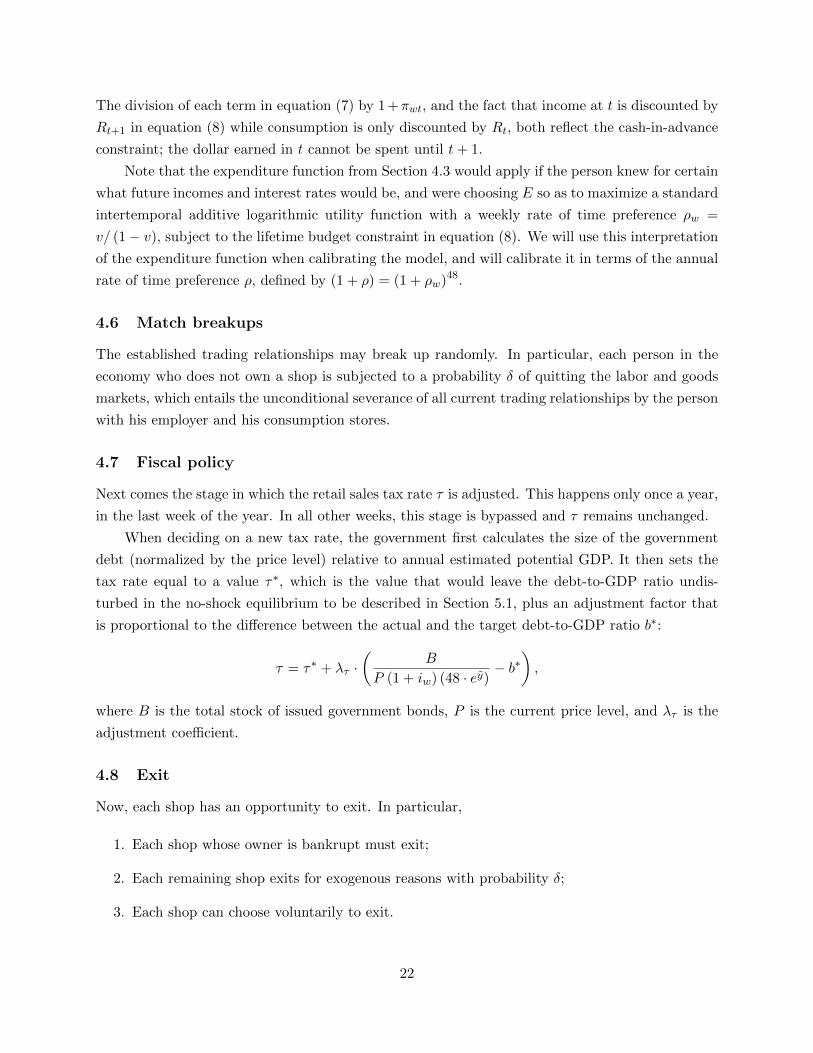
We assume that a shop will voluntarily exit with certainty if it cannot afford to pay for the

coming week’s fixed overhead cost, that is, if

A+ CL < w (F − 1) ,

where A is the shop owner’s financial wealth, computed as in Section 4.3 above.

The only other situation in which a shop will voluntarily exit is if it is unprofitable, in which

case it will exit with a fixed probability φ. In computing profitability, the shop owner takes into

account the opportunity cost of his labor services, that could be earning a wage, and the interest-

opportunity cost of maintaining the shop’s fixed capital and inventory. Specifically, the shop owner

will decide that the shop is unprofitable if one of the following two cases applies:

(a) A+ Pf (I + S) > 0 and V ·W + Pf (I + S) > V ·Πe;

(b) A+ Pf (I + S) < 0 and V ·W > V ·Πe +A,

where I is the shop’s inventory, S is his fixed capital, W is the current economy-wide average wage,

Pf is the firesale price, V is the capitalization factor, and Πe is the shop owner’s permanent income

(expected profit from staying in business). Each case implies that the owner’s tangible plus human

wealth would increase as a result of exit, under the assumption that he could get a job paying the

wage W . In case (a) he would be able to repay his loan in full, although perhaps allowing some

inventory and fixed capital to be seized, so in the event of exit his tangible plus human wealth

would go from V · Πe + A to V ·W + Pf (I + S) + A. In case (b) he would be unable to repay his

loan in full, so upon exit his tangible plus human wealth would go from V ·Πe +A to V ·W .

Once a shop exits for any reason, all trading relationships (with both employees and customers)

are dissolved and the shop owner has to repay his bank loan to the extent possible (bankrupt shops

have already settled their loans). If the sum of shop owner’s money and deposits exceeds the bank

loan, he repays the whole loan to the bank. Otherwise, the bank seizes capital as described in

Section 4.3 above, evaluating the capital at firesale prices. Banks with seized capital and former

shop owners with non-seized capital now join the appropriate firesale queues if not already there.

Upon exit, the former shop owner resets his permanent income to W .

4.9 Wage and price setting

In the final stage of weekly activities, each shop has an opportunity to update its posted wage and

retail price. Wage and price changes are not communicated automatically to the shop’s employees

and customers until the start of next period’s trading.

Each shop first updates its sales target ytrg, setting it equal to the current week’s actual sales.

Then, it proceeds to update the shop’s wage, but only if the last wage change was ∆ weeks ago,

where the length ∆ of the contract period is a parameter of the model. Given that the current

23

week is indeed a wage-updating week for the shop being considered, its wage is set equal to

w = w ·[(

1 + β ·(xtrg/xpot − 1

))· (1 + π∗)

]∆/48,

where w is the pre-existing wage, xtrg is the average input target over the past ∆ weeks, and xpot is

the average potential input over the same period (i.e., the number of people having an employment

relationship with the shop, even if they were laid off or if they refused to work because they were

not paid).16 The parameter β hence indexes the degree of wage and price flexibility in the economy.

This wage adjustment anticipates inflation over the coming contract period at an annual rate equal

to the CB’s target π∗.

Every week, each shop has an opportunity to revise its retail price. Its “normal” price is

pnor = (1 + µ)w/ (1− τ), which would equate its after-tax price to its wage times its desired

markup, corresponding to the rule discussed earlier in Section 4.1. The shop will choose this normal

price unless its inventories are too far from the desired level, namely its target sales. Specifically,

it will set

p =

pnor · δp, if I > ytrg · IS;

pnor · δ−1p , if I < ytrg · IS−1;

pnor, otherwise.

Thus, the frequency of price change will be endogenous. A shop will change its posted price almost

certainly twice a year, when its wage is changed and when the tax rate τ changes, because in both

cases its normal price will change. Beyond that, it will only change the price when its inventory-to-

sales ratio passes one of the critical thresholds IS and 1/IS. When the ratio rises above the upper

threshold, the shop cuts its price by the factor δp. When the ratio falls below the lower threshold,

it raises its price by the factor 1/δp.

4.10 Information and expectations

Public information. It follows from the preceding description of the interaction protocol in

our model that every agent is always fully informed of the following public variables: last week’s

economy-wide average wage rate W ; the most recently computed price level P ; the current one-week

interest rate on government bonds iw; the central bank’s weekly inflation target π∗w; the technology

of operating a shop, including the cost parameters S and F ; the ad valorem sales tax rate τ ; the

capitalization factor V computed by the central bank; and the firesale price Pf .

Private information. In addition to this public information that every agent knows, every person

always knows the values of: his own holdings of money, deposits, and legacy capital; the inventory,

fixed capital, and bank loan of his shop if he is a shop owner; the identity and type of any shop with

which he has a trading relationship; the identity, currently posted loan, deposit interest rates, and

16In computing this expression, we use the maximum of xpot and the shop’s fixed cost F to avoid division by zerowhen potential employment falls to zero.

24

haircut price of his bank; and his bank’s equity and required capital if he is a bank owner. Moreover,

we assume that every person always remembers his permanent income Y p, which is updated every

period during the financial market stage, as well as his effective wage and the effective retail prices

for his primary and secondary consumption goods.

Expectations. As in most macroeconomic models, expectations of inflation and of interest rates

play an important role in people’s demand behavior. We suppose that the central bank plays a

key role in anchoring these expectations, and that expectations play a benign role in aggregate

fluctuations. Specifically, as described in Section 4.9, when shops set wages they expect inflation to

proceed over the course of the contract period at a steady rate equal to the central bank’s inflation

target π∗.

In addition, from time to time, people want to estimate the current or future value of some

variable (wage, price, or income) knowing only what it was last period. In those cases, they simply

project the last known value into the future, assuming a constant weekly rate of inflation equal to

π∗w = (1 + π∗)1/48 − 1.

The other place where inflation expectations are critical is in the formation of household

expenditure plans. In this case, we suppose again that households rely on the central bank for

making forecasts, in the form of the capitalization factor V computed from the central bank’s

projections.

5 The workings of the model

5.1 Equilibrium with price flexibility and no shocks

As the preceding discussion has made clear, all shocks in this economy are individual shocks.

Unlike in the standard New Keynesian framework, we have postulated no exogenous shock process

impinging on aggregate productivity, price adjustment, aggregate demand, monetary policy, or

fiscal policy. Nevertheless, the individual shocks that cause matches to break up and shops to enter

or leave particular markets do have aggregate consequences because there is only a finite number

of agents. So, in general the economy will not settle down to a deterministic steady state unless

we turn off these shocks. If we do turn off all shocks, there is a deterministic equilibrium that the

economy would stay in if left undisturbed by entry and breakups (i.e., if θ = δ = 0), with wages

being adjusted each week (∆ = 1). This equilibrium will serve as an initial position for all the

experiments we perform on the model below, and a brief description of it helps to illustrate the

workings of the model.

The equilibrium is one in which all the potential gains from trade are realized. Each person is

matched with one employer and two stores. There are n shops, one trading in each of the n goods.

To preserve symmetry across goods, we suppose that each good is the primary consumption good

for exactly one shop owner. Each shop begins each week with actual, potential, and target input

all equal to n− 2, which is the number of suppliers of each good, and with actual and target sales

25

equal to inventory holdings equal to actual output: n − 2 − F . Thus, the economy’s total output

equals full capacity: y∗ = n (n− 2− F ).

Each shop begins each week with a common wage rate equal to W = (1 + π∗w)W0, where W0

was the common wage rate last week, and with a retail price equal to P = (1+ µ)W/ (1− τ), where

the tax rate τ equals

τ∗ = 1− (1 + π∗w) (1− 48ρwb∗) ·(

1− π∗wn− 3

(n− 2− F ) (1 + µ)

)−1

.

As mentioned earlier in Section 4.7, this is the tax rate that leaves the government’s real debt-to-

GDP ratio undisturbed in this equilibrium. We are assuming that all markups in this equilibrium

are equal to the average µ.

In this no-shock equilibrium there are no bank loans outstanding, so banks are just conduits,

converting deposits into government bonds. The initial outstanding stock of bonds is

B = b∗ (1 + iw) 48y∗P0,

where P0 = P/ (1 + π∗w) is last week’s price level. These bonds are held equally by all banks, and

each non-bank-owning person holds the amount B/N of bank deposits. The weekly interest rate

iw is given by

1 + iw = (1 + ρw) (1 + π∗w) .

The money supply at the start of the week is

M = W0 (N − n) + (1− τ)P0y∗,

which is the sum of all wage receipts of people not owning a shop, and all sales receipts (ex taxes)

of shop owners, from last period.

Each person starts the period with an effective wage equal to W0, and with effective retail

prices for both consumption goods equal to P0. The owner of each shop starts with a permanent

income equal to last week’s profit

Π = [(µ− iw) (n− 2− F )− (1 + iw) (F − 1)]W0,

and with money holding equal to last week’s revenue (1− τ)P0 (n− 2− F ). Each person not

owning a shop begins with money holding equal to permanent income, which in turn is equal to

last period’s wage income W0.

No one holds any legacy capital, no banks hold seized capital, and the firesale queues are all

empty. Banks hold no reserves, so each bank’s equity is its share of the government debt minus its

customers’ deposits, which amounts to B/N .

26

The initial history is one in which the output gap has been equal to zero for the past 12

months and inflation has equaled its target rate for the past 12 months. The central bank’s real

interest target is r∗ = ρ, and its estimate of log potential GDP is y0 = ln (y∗). Its latest published

capitalization factor is

V =1

1 + π∗w· 1

ρw.

It is straightforward to verify that this configuration will repeat itself indefinitely, with all

nominal magnitudes – money and bond holdings, actual and effective wages and prices, and per-

manent incomes – rising each week at the constant rate π∗w, provided that the setup cost F is small

enough that shops always pass the profitability test during the exit stage, which indeed it is in the

baseline calibration described in Section 6 below.17

5.2 Entry, exit, and systemic performance

As we shall see below, on average, the economy is able to achieve about 93 percent of the capacity

GDP attained in the no-shock equilibrium. GDP goes down whenever a shop that was satisfying

some consumers goes out of business or a customer loses a store because of a random breakup.

GDP also goes down whenever a new shop enters and diverts workers from old shops that were

satisfying some customers, because some of these workers’ efforts will be used up in deferring the

fixed cost of the new shop rather than producing goods that can be eaten by customers of the old

shop.

These events that reduce GDP are constantly being offset to some degree by the entry of new

shops that are able to satisfy customers in markets where there had previously been no viable

shop, and by the exit of shops that were using up fixed costs but not producing enough to satisfy

their customers. Thus, both entry and exit are critical to the system’s ability to approximate full-

capacity utilization. However, although entry of new shops is useful in markets where there are no

incumbents, or where the incumbents are not hiring all the potential workers because of layoffs or

because of financial problems that prevent them from meeting their payroll, entry can be harmful

(to the level of real GDP) in cases where incumbent shops were hiring most of the potential workers

and satisfying most of the potential customers. Likewise, although exit is important in cases where

the shop has ceased to play an active intermediation role, whether because of financial difficulties,

a surfeit of inventories, or a too high markup, exit can also be very harmful in cases where the

incumbent was previously doing well, because it can cascade across markets causing a cumulative

loss of output (see Howitt, 2006).

Banks have two influences on this cumulative process of shop failures. One is the familiar

“lending channel” of the financial accelerator. That is, when a shop fails, this may cause its bank

to get into trouble, or at least to get close to being in trouble, because some of its loans may go

bad. This will cause it to lend less readily, either by reducing its probability of approving credit

17In our baseline calibration F = 3.5, whereas the critical value F ∗ at which the profitability test fails is 63.

27

line applications or, in the extreme case, by having the government forbid it from making any new

loans. This makes it more likely that other firms will fail for lack of finance.

The other influence that banks have is a more salutary one of ameliorating the cumulative

process. That is, the cascade of shop failures will be dampened if another shop quickly replaces

each failed shop. This is more likely to happen when banks are willing to lend because bank lending

makes it easier to pass the financial viability test at the entry stage each week.

As we shall see, it seems that the latter effect of banks, facilitating entry, appears to play a

more important role in our model, especially when the system is far below full-capacity utilization,

than the more traditional accelerator role, in the sense that banks dampen shocks and allow the

economy to achieve on average a higher degree of capacity utilization.

6 Calibration

Although the model has many agents, we have imposed a great deal of ex ante symmetry. We have

done this partly to be able to fully characterize the no-shock equilibrium that serves as a reference

point, which will facilitate our analysis of what is generating the experimental results, and also

partly to keep the number of parameters small enough to calibrate them to U.S. economic data.

This section describes our calibration procedure.

There are a total of 33 parameters, which we have categorized as personal parameters, shop

parameters, bank parameters, and government policy parameters. These are listed in Table 1 along

with their assigned values and the six-letter codes to be used further below in the sensitivity analysis

in Section 9.

Our calibration of these parameters took place at three different levels. At the first level, one

subset of parameter values was chosen to match their empirical counterparts in the U.S. data and/or

the values used in previous studies. At the second level, the values of other parameters were chosen

so as to be internally consistent with median outcomes across simulations. At the third level, the

values of the remaining parameters, for which we could find no convenient empirical counterparts,

were chosen to make their median outcomes across simulations (loosely) match certain properties

of the U.S. data.

6.1 First level of calibration

6.1.1 Personal parameters

We set the annual rate of time preference ρ equal to 0.04 as is standard in the real business cycle

literature. We chose the demand parameter ε to equal 7, which implies that the elasticity of demand

facing each shop would be 1+ε/2 = 4.5 in a no-shock equilibrium with all shops charging the same

price. This lies in the range of values typically found in New Keynesian DSGE models.18 However,

18Demand elasticity is set equal to 3 in Midrigan (2011), 4 in Nakamura and Steinsson (2010), and 7 in Golosovand Lucas (2007). The benchmark calibration in Burstein and Hellwig (2008) yields an elasticity of 4.4.

28

Table 1: The calibrated parameters of the model

Personal parameters

ρ Rate of time preference (annual) 0.04 TMPRFYε Demand parameter 7.0 DMDELSδ Quit rate (weekly) 0.00075 BRKFRCλp Permanent income adjustment speed (weekly) 0.4 INCSPDσ Job search probability 0.5 SRCHPPθ Frequency of innovation (weekly) 100 INFREQ

Shop parameters

∆ Length of the contract period (in weeks) 48 CNTPRDF Fixed cost (weekly) 3.5 FXDCSTλI Inventory adjustment speed (weekly) 0.16 INVSPDβ Wage adjustment coefficient (annual) 0.3 WAGSPDµ Average percentage markup over variable costs 0.138 MARKUPφ Failure rate of unprofitable shops (weekly) 0.011 FAILRTS Setup cost 15 SETUPCIS Critical inventory-to-sales ratio 3.0 TRIGGRδp Size of price cut (old price/new price) 1.017 PDELTA

Bank parameters

s Loan spread (annual) 0.0175 SPREADCb Cost of foreclosure 0.1 BKRCSTl Slope of loan approval schedule 9 PSLOPE

Government policy parameters

Fiscal policyb∗ Target debt-to-GDP ratio 0.33 BNDINCλτ Fiscal adjustment speed (annual) 0.054 FSCSPD

Monetary policy

λπ0 Inflation autocorrelation coefficient (initial estimate) 0.29 INFCOR

λy0 Output autocorrelation coefficient (initial estimate) 0.66 GAPCORγπ Inflation coefficient in Taylor rule 1.5 INFTYRγy Output gap coefficient in Taylor rule 0.5 GAPTYRπ∗ Target inflation rate (annual) 0.03 PITRGYr∗0 Initial target real interest rate (annual) 0.032 RRTTRGy0 Initial estimate of potential output 7.6 GAPTRGηr Adjustment speed of evolving real rate target 0.0075 ADJRRTTcb Number of years before CB’s learning begins 10 LRNLAG

Bank regulationκ Required capital adequacy ratio 0.08 CARATEsd Premium on CB’s discount rate (annual) 0.005 DISCPRm Number of banks 5 NBANKSh Loan-to-value ratio 0.5 LVALRT

29

the elasticity of demand faced by a shop out of equilibrium, when he has rivals selling the identical

good, will be larger than 4.5 because raising the retail price may induce a loss of all demand from

any customer that finds another shop during the matching process.19

6.1.2 Shop parameters

Smets and Wouters (2007) estimate the average duration of wage contracts in the U.S. to be about

a year. This is consistent with evidence from other studies cited in Amano et al. (2009, section 4).

Accordingly, we set the length of the wage contract period ∆ to 48 weeks, which in our model is

one year.

Estimates of the degree of returns to scale in the U.S. economy vary from 0 to about 30 percent.

It is commonly measured as the ratio of average to marginal cost (minus unity). In our model, the

typical shop in a steady state with input equal to x and sales equal to x − F would thus have a

degree of returns to scale equal to

AC

MC− 1 =

Wx/ (x− F )

W− 1 =

F

x− F.

If the economy was operating with a 6 percent average unemployment rate, then the typical shop

would have x = 0.94 · (n− 2) = 45.12, so by setting the fixed cost F equal to 3.5 we get a typical

degree of returns to scale equal to 8.4 percent.

The inventory adjustment speed λI = 0.16 corresponds to the estimate by Durlauf and Maccini

(1995) of a monthly adjustment speed equal to 1− (1− 0.16)4 ≈ 0.5.

Roberts (1995) estimated aggregate expectations-augmented Phillips relations with a coeffi-

cient on detrended output between 0.25 and 0.334 using annual data. A linear approximation to

our wage-adjustment equation yields the same relation at the firm level if we assume that the

actual/capacity output ratio is proportional to the target/potential input ratio. Accordingly, we

chose β = 0.3 to lie near the midpoint of Roberts’ range of estimates.

6.1.3 Bank parameters

The value of the normal annual loan spread s was set equal to 0.0175, which is the average spread

between lending and deposit rates for all commercial and industrial loans during the period 1986–

2008. This figure comes from the Survey of Business Lending Terms conducted by the Federal

Reserve.

We set the cost of foreclosure equal to 0.1, which falls in the 2 percent to 20 percent range

suggested by Bris et al. (2006).

19This is another consequence of our decision to model goods markets as “customer markets” after Phelps andWinter (1970).

30

6.1.4 Government Policy parameters

Fiscal policy. The target debt-to-GDP ratio b∗ was set equal to 0.33 because this is the average

ratio of federal marketable debt to GDP in the U.S. between 1969 and 2005. The fiscal adjustment

speed λτ was estimated at 0.054 by Bohn (1998).

Monetary policy. The initial estimates of the autocorrelation factors λπ0 and λy0 were taken from

estimates of univariate AR(1) processes on inflation and on (linearly detrended) log per-capita GDP

using annual data for the U.S. over the 1984–2006 period. The coefficients γπ and γy are Taylor’s

original specification. We took the inflation target π∗ to equal 3 percent, which is the average in

the U.S. over the 1984–2006 period.

Bank regulation. We set the required capital adequacy ratio κ equal to 0.08, which corresponds to

the Basel I capital accord. The CB’s discount rate premium sd is set to 0.005, which approximates

the typical spread of the Federal Reserve’s primary credit discount rate over the federal funds rate.

6.2 Second level of calibration

6.2.1 Government targets – finessing Wicksell

The two government policy targets – the target real interest rate r∗ and log potential output y –

are chosen adaptively by the government. We chose the initial value of r∗ to be 0.032, which is

close to the steady-state value, on average across simulations, in our baseline calibration. Likewise,

we choose the initial value of y0 to be 7.6, which is its median value20 across simulation runs in our

calibration exercise. Since government adaptation was relatively quick, and its learning period was

quite long, our results were not sensitive to the choice of these initial values.

Note that our procedure of having the government estimate r∗ and y forces it to deal with the

danger that writers from Wicksell to Friedman and up through Orphanides have warned of – the

danger that no one knows the economy’s natural rate of interest or potential output, and hence

that controlling the rate of interest to the neglect of the money supply risks aggravating volatility

or even engendering cumulative inflation.

6.2.2 Markups and the Lucas Critique

In early trials with the model, we assumed that all shops applied the same markup. But we found

that the results of many experiments were highly sensitive to the assumed size of the markup.

Awareness of the Lucas critique prompted us to revise the model in favor of the current assumption,

namely that each shop picks its markup at birth. This variant allows the economy-wide average

markup to respond endogenously to the policy environment, through the evolutionary selection

mechanism implicit in the exit process. We chose the mean of the distribution from which markups

20This corresponds to the logarithmic output gap (between capacity GDP and actual GDP) of 0.074 reported inTable 3.

31

Table 2: U.S. data vs. median outcomes in the model

Variable Data Model

Inflation 3.0 2.9Real interest rate 1.8 3.2Unemployment rate 6.1 5.9Unemployment duration 14 10Volatility of output gap 2.0 to 3.2 2.8Volatility of inflation 1.3 0.69Autocorrelation of gap 20 to 76 43Autocorrelation of inflation 16 19Average markup 10 to 20 14Exit rate 46 40Job loss rate 0.69 0.59Price-change frequency 4.0 4.1Annual bank failure rate 0.51 0.50

are drawn in the same way that we decided on the initial values of the government targets – by

internal consistency. The median markup across simulation runs in our baseline calibration exercise

is about 0.138 when shops choose from a distribution whose mean µ is 0.138.

6.3 Third level of calibration

This leaves 13 parameters still to be determined, namely φ, S, IS, δp, δ, λp, σ, θ, l, ηr, Tcb, m,

and h. These were chosen by searching (manually) for parameter values that would make the

values of thirteen different indicators in our model approximate their counterparts in the U.S. data.

More specifically, we ran 10,000 simulations of 60 years. Each simulation run started near the

no-shock equilibrium and continued for 20 years before we started calculating the average value

of each indicator variable across the remaining 40 years of that simulation. For each variable, we

then computed the median across all simulation runs of these cross-year averages. The thirteen

indicator variables are listed in Table 2, along with their actual values from U.S. data and their

median values in our fully calibrated model.

All numbers are expressed in percentage points, except for unemployment duration, which is

expressed in weeks, and price-change frequency, which is expressed in number of changes per year.

The actual values from U.S. data for these thirteen indicators were determined as follows. The

real annual interest rate is computed as the difference between the annual interest rate on 3-month

T-bills (monthly data from the Federal Reserve) and the CPI inflation rate (monthly data from

the U.S. Bureau of Labor Statistics), averaged over the period 1984–2006. Unemployment rate

and duration are the averages over the period from 1969 to 2009. The volatility of the output

gap is the standard deviation of linearly detrended and HP-filtered log per-capita GDP, and the

volatility of inflation is the standard deviation of annual U.S. CPI inflation over the 1969–2009

period. The autocorrelations of these two variables are computed by estimating an AR(1) process

32

over the same time period. Golosov and Lucas (2007) indicate that estimates of the percentage

markup vary between 10 and 20 percent. The exit rate is the fraction of all shops found operating

in a given industry in one census year that are found still operating in that industry in the next

census year (five years later), which Dunne et al. (1988) report to be 46.4 percent. The job loss rate

is the weekly rate of job loss that would give rise to the number reported by Hall (1995), namely

that 71.8 percent of people working at a given date have been working continuously for the same

employer for the past year.21 Bils and Klenow (2004) find an average price-change frequency of 16

weeks, which in our model would imply an average annual price-change frequency of 3. However,

in our model, shops will almost always change prices every time there is a change in the sales tax,

which is once per year, whereas in reality sales tax changes are very infrequent. Thus, we aimed

to match a price-change frequency of 4. Finally, according to the FDIC (Historical Statistics on

Banking), the average commercial bank failure rate was about 0.51 percent per year over the period

from 1984 to 2006.

As Table 2 shows, we were mostly successful in mimicking the data with our 13 parameters.

Specifically, our model underpredicts the duration of unemployment, the volatility of inflation, the

job loss rate, and the exit rate.

7 Simulating the model

Each simulation run of the model is allowed to continue for T = 2880 weeks (60 years). We repeat

this for R = 10, 000 runs. Each run starts off near the flexible-price no-shock equilibrium described

in Section 5.1 above. We do not start tabulating results from each run until 20 years have passed,

so as to allow the system time to settle into a stochastic steady state. As Figure 1 shows, our

20-year adjustment period was indeed enough for the cross-run average values of the output gap

(measured as the difference between log capacity GDP and log actual GDP), the real interest rate,

and the inflation rate to become more or less constant, except for the slight downward trend in the

cross-run average gap over the first half of the final 40-year period. The figure shows the average

value at each year across all 10,000 runs, with the output gap measured on the left-hand axis, and

the real interest rate and inflation rate on the right-hand axis.

7.1 Normal times and bad times

Most of the simulation runs produced time paths that exhibit strong homeostatic tendencies. How-

ever, as indicated in our introductory remarks, there are also a few “pathological” runs in which the

market makers appear to have lost control of the system. This is an important nonlinear feature of

the model, which seems to behave in a qualitatively different manner in bad times as compared to

normal times. To convey some idea of this qualitative difference, Figure 2 depicts the actual time

21That is, (1 − α)48 = 0.718 if α = 0.00688.

33

.01

.02

.03

.04

.05

Infla

tion

rate

, rea

l int

eres

t rat

e

.05

.075

.1.1

25.1

5

Out

put g

ap

10 20 30 40 50 60

Year

Output gap Inflation rate Real interest rate

Figure 1: Time series of the cross-run averages

path of three major macroeconomic variables in one of the many “normal” runs of the system.22 A

randomly chosen simulation would almost certainly depict similar characteristics. There are times

when the output gap rises for a few years, but these times are soon followed by recovery. The

output gap rarely exceeds 0.2.

In contrast with these normal runs, Figure 3 illustrates what happens in some of the “worst

decile” of runs, that is, in runs belonging to the first decile of the distribution across all 10,000 runs

of the 40-year average output gap. Again, there are times when the output gap rises for a year or

two, but beyond some point it breaches the usual upper limit of 0.2 and shows no tendency to return

to anything like the cross-run average of 0.074. Indeed, there were 4 runs out of 10,000 in which

the output gap became infinite (GDP = 0) in finite time.23 Although we have not investigated

the matter in a rigorous statistical sense, we doubt that such behavior could be produced by any

known linear macro model. These collapses suggest the presence of something like Leijonhufvud’s

(1973) “corridor;” it seems as if the economy is capable of absorbing shocks up to some limit but

not beyond.

22The “rnseed” number in each figure caption indicates the initial seed value of the random number generator forthe depicted run.

23We excluded these runs from the computation of the cross-run average paths shown in Figure 1.

34

−.0

20

.02

.04

.06

Infla

tion

rate

, rea

l int

eres

t rat

e

0.0

5.1

.15

.2

Out

put g

ap

10 20 30 40 50 60

Year

Output gap Inflation rate Real interest rate

Figure 2: A normal run (rnseed = 17)

−.0

50

.05

Infla

tion

rate

, rea

l int

eres

t rat

e

0.5

11.

5

Out

put g

ap

10 20 30 40 50 60

Year

Output gap Inflation rate Real interest rate

Figure 3: A collapse (rnseed = 5340)

35

2040

6080

100

Per

cent

, rel

ativ

e to

the

wor

st d

ecile

1 2 3 4 5 6 7 8 9 10

Decile

Job loss rate Unemp. duration Inflation volatility Output gap

Unemp. rate Output volatility Banks in trouble

Figure 4: Macro performance by decile

7.1.1 The anatomy of bad times

Figure 4 indicates the average behavior of various macro performance measures by decile of runs,

where the runs are ordered in terms of their cross-year average output gap.24 As illustrated by the

figure, with the exception of the job loss rate, there is a sharp deterioration in all these measures

in the tenth decile.25

To some extent, this deterioration is just what one would expect from a more standard New

Keynesian DSGE model that respected the zero lower bound on nominal interest rates.26 Indeed,

as Figure 5 shows, the fraction of times in which the zero lower bound is hit rises sharply from

0.035 in the ninth decile to 0.114 in the tenth.

However, there is more going on. Figure 6 reports the results of redoing the 10,000 simulation

runs of our basic calibration, but allowing the nominal interest rate to be determined by the Taylor

rule even when this rule would make it negative. All other behavioral rules in the model were left

unchanged. Of course, this experiment begs the question of why people would aim to have their

cash-in-advance constraints binding when the nominal interest rate was below zero, but it does

24Each performance measure is its mean value during the final 40 years of a run, averaged across runs specific toa given decile.

25The variables consist of those listed in Table 3, except for the rate of inflation and the incidence of bank failure.As we argue below, inflation tends to move in the opposite direction to the other indicators, while bank failures inthe model are salutary events.

26See, e.g., Eggertsson and Woodford (2003) or Levin et al. (2010).

36

0.0

4.0

8.1

2

Zer

o lo

wer

bou

nd h

its, f

ract

ion

of ti

mes

1 2 3 4 5 6 7 8 9 10

Decile

Figure 5: Frequency of hitting the zero lower bound

2040

6080

100

Per

cent

, rel

ativ

e to

the

wor

st d

ecile

1 2 3 4 5 6 7 8 9 10

Decile

Job loss rate Inflation volatility Unemp. duration Output gap

Unemp. rate Output volatility Banks in trouble

Figure 6: Decile-by-decile performance without the zero lower bound

37

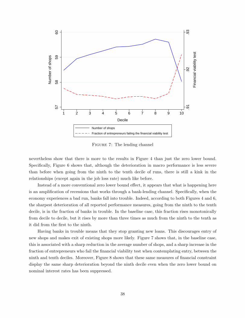
.91

.92

.93

Fin

anci

al v

iabi

lity

test

5758

5960

Num

ber

of s

hops

1 2 3 4 5 6 7 8 9 10

Decile

Number of shops

Fraction of entrepreneurs failing the financial viability test

Figure 7: The lending channel

nevertheless show that there is more to the results in Figure 4 than just the zero lower bound.

Specifically, Figure 6 shows that, although the deterioration in macro performance is less severe

than before when going from the ninth to the tenth decile of runs, there is still a kink in the

relationships (except again in the job loss rate) much like before.

Instead of a more conventional zero lower bound effect, it appears that what is happening here

is an amplification of recessions that works through a bank-lending channel. Specifically, when the

economy experiences a bad run, banks fall into trouble. Indeed, according to both Figures 4 and 6,

the sharpest deterioration of all reported performance measures, going from the ninth to the tenth

decile, is in the fraction of banks in trouble. In the baseline case, this fraction rises monotonically

from decile to decile, but it rises by more than three times as much from the ninth to the tenth as

it did from the first to the ninth.

Having banks in trouble means that they stop granting new loans. This discourages entry of

new shops and makes exit of existing shops more likely. Figure 7 shows that, in the baseline case,

this is associated with a sharp reduction in the average number of shops, and a sharp increase in the

fraction of entrepreneurs who fail the financial viability test when contemplating entry, between the

ninth and tenth deciles. Moreover, Figure 8 shows that these same measures of financial constraint

display the same sharp deterioration beyond the ninth decile even when the zero lower bound on

nominal interest rates has been suppressed.

38

.91

.92

.93

Fin

anci

al v

iabi

lity

test

5758

5960

Num

ber

of s

hops

1 2 3 4 5 6 7 8 9 10

Decile

Number of shops

Fraction of entrepreneurs failing the financial viability test

Figure 8: The lending channel without the zero lower bound

8 Analyzing the role of banks

8.1 Banks, no banks, and “risky” banks

As mentioned in the introduction to the paper, our results indicate that banks do matter for

macroeconomic performance, especially when times are extremely bad, and that in bad times they

are especially helpful when they are riskier from the perspective of micro-prudential regulation,

that is, when they have higher loan-to-value ratios and lower capital adequacy ratios.

In order to gain more insight into how banks affect median performance across runs, we per-

formed an experiment of shutting down all banks and rerunning the simulations underlying our

baseline calibration. To do this, we simply changed the banks’ behavior in the financial market

stage of each week so that they always imposed a credit limit of zero on all customers. This turns

banks into mere conduits for the private holding of government debt. In this experiment, a bank’s

equity is equivalent to deposit holdings of its owner, and its risk-weighted assets (loans and seized

collateral) will always be zero, so the bank will never fail and will never be in trouble.

The results of this experiment can be seen in the first two columns of Table 3, which reports

the medians across simulations of the averages across years of different performance indicators. As

39

Table 3: Median outcomes

Variable Banks No banks Risky banks

Inflation 2.9 2.5 3.0Output gap 7.4 13 7.5Unemployment rate 5.9 11 5.8Unemployment duration 10 19 8.7Job loss rate 0.59 0.68 0.69Volatility of output gap 2.8 6.2 2.5Volatility of inflation 0.69 1.2 0.61Annual bank failure rate 0.5 0 2.5Fraction of banks in trouble 4.6 0 1.1

is evident from the table, with the exception of inflation, all indicators show a marked deterioration

in median performance when banks are shut down.27

We get another measure of the importance of banks by simulating the economy’s response to

various exogenous shocks. Figure 9 shows the average response of the economy to a shock in which

one of the five banks is forced to be in trouble for one year. Specifically, at the beginning of year

20 in the simulation (i.e., at the end of the adjustment period to a steady state), we impose on the

first of the five banks the restriction that it cannot initiate new loans and cannot pay dividends

to its owner, independently of its capital adequacy. We repeat this simulation 10,000 times. For

a counterfactual, we perform the same 10,000 simulations, with the same sequence of seeds for

the random number generator, but without the shock that forces a bank into trouble. The lower

(“safe” banks) line in Figure 9 indicates the “trimmed” average difference in log GDP between the

shocked and counterfactual simulations on a monthly basis for two years (24 months) following the

shock.28 The effect is not huge, never exceeding one percent of the average counterfactual value,

but it is persistent.

Another experiment we ran was to force a shop to fail. We did this both with and without

banks. Figure 10 shows that in either case there was a humped-shape impulse response of log

GDP, which is much stronger in the economy without banks (the upper curve) than in the baseline

(“safe” banks) scenario. As explained by Howitt (2006), in a much simpler model based on the

same foundations, the exit of a shop can cause a cumulative fall in output by depriving the shop’s

former suppliers of their source of income and thus endangering other shops from loss of demand.

Each time a shop fails, aggregate output falls automatically by an amount equal to that shop’s

employment less its fixed overhead cost, unless it was already employing too few workers to cover

its fixed cost. The process continues until the former employees of failed shops find new employers,

27Inflation is lower because the fact that firms always factor in the same target inflation rate π∗ when adjustingwages means there is a long-run tradeoff between output and inflation.

28That is, in order to avoid the noisiness of runs where either the shocked or counterfactual simulation spun out ofcontrol, we calculated, for each month, the average between the 25th and 75th percentile of all these differences.

40

0.0

05.0

1.0

15

Diff

eren

ce in

log

GD

P

0 5 10 15 20 25

Month

Safe banks Risky banks

Figure 9: Average response to a troubled bank shock

0.0

05.0

1.0

15.0

2

Diff

eren

ce in

log

GD

P

0 5 10 15 20 25

Month

Safe banks Risky banks No banks

Figure 10: Average response to a shop failure

41

Table 4: Worst-decile average outcomes

Variable Banks No banks Risky banks

Inflation 2.7 1.4 2.9Output gap 11 44 9.3Unemployment rate 8.9 28 7.2Unemployment duration 13 27 9.9Job loss rate 0.69 1.9 0.76Volatility of output gap 5.2 23 3.4Volatility of inflation 0.94 1.8 0.68Annual bank failure rate 1.4 0 3.1Fraction of banks in trouble 13 0 1.7

and this will often require new shops to enter. As Figure 10 shows, banks play an important role

in mitigating the multiplier process of cascading shop failures by facilitating new entry.

This last experiment suggests that banks should make an even bigger difference in bad times

than in normal times. As we have seen, bad times are exacerbated by a loss of shops, which can

be mitigated by bank lending that facilitates entry, whereas, as argued above, entry is less critical

when the economy is already near a situation of full-capacity utilization. Table 4 reveals that banks

do indeed make a bigger difference in bad times. It shows the average values of various performance

measures across the worst decile of runs, with and without banks. In almost all cases, the difference

in worst-decile averages between the two scenarios is considerably larger than the corresponding

difference in medians reported in Table 3. For example, banks reduce the median unemployment

rate from 11 to 5.9 percent, but they reduce the worst-decile average unemployment rate from 28

to 8.9 percent.

8.1.1 Risky banks

To gauge how much of a difference bank regulation will make, we consider an alternative scenario

with “risky” banks, which differs from our baseline scenario with “safe” banks in two senses. First,

instead of constraining its customers with a haircut price equal to the firesale price (i.e., with a

loan-to-value ratio of 0.5), each bank in this risky scenario allows a higher loan-to-value ratio of

0.9. Second, we suppose that the required capital adequacy ratio is just 0.02, rather than the more

credit-constraining value of 0.08.

As the third column of Table 3 indicates, macro performance under the risky scenario is roughly

comparable to performance under our baseline safe scenario. Median unemployment is about the

same, as is the median output gap, but volatility and unemployment duration are lower while the

job loss rate is higher. As expected, the incidence of bank failures is much higher and, because

trouble is defined more loosely for a risky bank, the median fraction of banks in trouble is much

lower.

42

0.1

.2.3

Diff

eren

ce in

the

num

ber

of e

ntra

nts

0 5 10 15 20 25

Month

Safe banks Risky banks No banks

Figure 11: Average response of entry to a shop failure

However, as Table 4 indicates, worst-case performance is considerably better under the risky

scenario than with safe banks. This is clearly because the critical role that banks play in mitigating

bad times is to facilitate the entry of new shops by their willingness to lend. Risky banks will perform

this role better than safe banks because their higher loan-to-value ratio makes them automatically

willing to lend more when they are not in trouble. In addition, their lower capital asset ratio means

that they are less often in trouble and hence less often unable to lend.

These insights are corroborated by Figure 10, which shows that the hump-shaped impulse

response of GDP to a shop failure is more moderate with risky banks than with safe ones. On the

other hand, Figure 9 shows that a troubled-bank shock has a larger output effect under the risky

scenario, which is hardly surprising because the bank that falls into trouble cuts its lending from

a larger average amount when risky than when safe. But this amplification of the troubled-bank

shock is mitigated by the fact that banks are less often in trouble in the risky scenario.

8.2 The financial accelerator and the financial stabilizer

The fact that shop failures make banks more likely to be troubled, which in turn makes shops more

likely to fail, means that in our model there is a financial accelerator that works through the bank-

lending channel. However, the fact that the economy is less volatile and performs better on average

by any measure with banks than without suggests that there must also be a “financial stabilizer” at

work whose effect is more powerful than that of the financial accelerator. As explained above, this

43

.07

.08

.09

.1.1

1.1

2

Log

outp

ut g

ap

.5 .6 .7 .8 .9

Loan−to−value ratio

Safe banks, worst decile Risky banks, worst decile

Safe banks, median Risky banks, median

Figure 12: Effect of loan-to-value ratio on output gap

is because of the way banks finance entry, an effect that is shown clearly in Figure 11. This figure

illustrates the average response of new entry, month by month, following a forced shop failure (in

the same experiment that underlies Figure 10). In all scenarios, entry rises following a shop failure

because more entrepreneurs are likely to pass the market research test when potential customers

and suppliers have just lost a shop. But the response is stronger in the baseline (safe-banks) scenario

than when there are no banks, and even stronger still in the risky-banks scenario.

8.3 Policy Experiments

Another way to see the difference between safe and risky banks is to conduct the following policy

experiment. We start with the safe scenario and increase the loan-to-value ratio gradually from 0.5

to the riskier value of 0.9, by increments of 0.1, while maintaining the required capital adequacy

ratio of 0.08. For each of the five indicated values of the loan-to-value ratio, the model was again

simulated 10,000 times. The same set of simulations was then repeated for the risky scenario,

that is, with the less credit-constraining required capital adequacy ratio of 0.02. Figure 12 shows

the results of this experiment. It illustrates that the increase in the loan-to-value ratio resulted

in a moderate deterioration of median performance (as measured by the output gap) under each

scenario but an improvement in worst-decile average performance that is especially pronounced in

the risky case. Again, this suggests that willingness to lend makes relatively little difference in

normal times but helps substantially when the economy is in trouble.

44

.06

.08

.1.1

2.1

4

Log

outp

ut g

ap

.02 .04 .06 .08 .1 .12 .14 .16

Capital adequacy ratio (intercept)

Safe banks, worst decile Risky banks, worst decile

Safe banks, median Risky banks, median

Figure 13: Effect of capital adequacy ratio on output gap

We also experimented with other policy interventions. Figure 13 shows the results from in-

creasing the required capital adequacy ratio gradually from 0.02 to the more credit-constraining

value of 0.16, by increments of 0.02, while maintaining the loan-to-value ratio at either 0.5 (for the

safe scenario) or at 0.9 (for the risky scenario). Here again, the figure demonstrates that there is

little effect on median performance but that worst-case performance is significantly degraded by

this tightening of regulation under both scenarios.

Several commentators have called for making capital adequacy requirements procyclical under

what is commonly known as macro-prudential regulation. To implement such a policy in our model,

we supposed that the capital adequacy rate κ is tied to the difference between log output and the

central bank’s estimate of log potential output. The adjustment is similar to that of the central

bank’s target interest rate and also employs a squasher. Specifically,

κ = κ+ ηκ (y − y) · f (y, κ) , f (y, κ) ≡ κ√η2κ (y − y)2 + κ2

,

where ηκ is a fixed capital adequacy ratio adjustment parameter and κ is the average required

capital adequacy ratio. The capital adequacy rate was adjusted according to this formula once a

month, at the time of the government’s interest setting decision. Figure 14 shows the results from

making the capital adequacy rate increasingly procyclical by varying the adjustment parameter

from 0 to 2.5. As before, we conducted simulations under both a risky scenario, that is, with an

45

.07

.08

.09

.1.1

1

Log

outp

ut g

ap

0 .5 1 1.5 2 2.5

Capital adequacy ratio (slope)

Safe banks, worst decile Risky banks, worst decile

Safe banks, median Risky banks, median

Figure 14: Effect of making the capital adequacy ratio procyclical

average capital adequacy ratio of 0.02 and a loan-to-value ratio of 0.9, and a safe scenario, where

the average capital adequacy ratio was set to 0.08 and the loan-to-value ratio was set to 0.5. As

depicted in Figure 14, the policy has almost no effect on the median output gap or on the worst-case

average performance under the risky scenario, but it does result in significantly better worst-case

performance under the safe scenario.

8.4 Making bank failure costly

The failure of a bank in our model is a salutary event. A bank that is about to fail is almost

certainly in trouble, not making any new loans, and is subsequently replaced by a new bank that

can resume making new loans. Thus, one reason for our finding that risky banks result in improved

macroeconomic performance is that their higher failure rate does not impinge negatively on the

real economy.

One argument for believing that bank failure does in fact impair macroeconomic performance

is that it may result in the loss of important information that the failing bank had regarding its

customers. In particular, a new bank may require some time to get to know the customer base,

and in the meantime it will not be as willing as the old bank would have been to extend credit

to customers that look like poor risks on the basis of the hard information that is available to an

outsider.

46

To explore this possibility, we changed the model along the following lines. In each market, we

designated N c of the n− 2 potential shop owners as “crooks.” We assumed that any bank that has

been in business for at least 48 weeks knows which of the agents in its sector are crooks and which

are not, but that a new bank cannot distinguish crooks from other customers until having been in

business for T c weeks. The new bank, however, does know the fraction of total loan applications

that are coming from crooks. Thus, when a bank fails, the replacement bank will charge a higher

loan interest rate in order to compensate for the predictable losses generated by fraudulent loan

applications.

More specifically, during the entry phase, if a crook becomes an entrepreneur, he asks his bank

for a line of credit. If the loan application is granted, he takes out a loan equal to the monetary cost

SN of his fixed capital minus his financial wealth, just like any other entrepreneur with the same

financial wealth and no legacy capital. However, unobserved by his bank, the crook will not open a

shop (we can assume that crooks do not even know how to open a shop). Instead, he deposits the

loan in his bank account and never repays any amount of the loan. The following week, the bank

will realize that he is a crook, but we assume that there is nothing the bank can do at this stage

other than write the loan down to zero in its books.

We also assume that crooks can never become bank owners. Given that crooks and other

non-bank-owning, non-shop-owning people have the same probability of becoming an entrepreneur,

the fraction of loan applications coming from crooks will be pc = NcnN−Ω−5 , where Ω is the number of

shops at the start of the week, assumed to be known by all banks. We further assume that a new

bank (i.e., one that has been in business for less than T c weeks) sets a loan rate iL such that its

expected return from a new loan is equal to iw + s/48, the loan rate of an experienced bank; since

the bank loses interest plus principal from each loan to a crook, this means that

iL =1 + iw + s/48

1− pc− 1.

At the beginning of the goods and labor market trading stage of each week, we assume that,

for each legitimate shop owner that applies for a loan to finance a firesale purchase, there is a

probability pc

1−pc that a crook will apply for a loan of the same size. Again, the new bank cannot

tell these fraudulent loan applications from legitimate ones, although it knows that the fraction pc

of such loans are being granted to crooks. We set the initiation period T c of a new bank equal to

48 weeks. Once the initiation period is over, the bank simply rejects all loan applications coming

from crooks.

In this variation of the model, the presence of crooks can make bank failure a problem since

now there will be a very high interest rate to be paid by new entrants and by established firms in

20 percent of the economy for a year following the exit of a bank. This could potentially reverse

our ranking of safe and risky banks, in terms of worst-decile macro performance, since risky banks

fail more often than safe banks.

47

Table 5: Worst-decile average outcomes with “crooks” in the model

Variable Banks No banks Risky banks

Inflation 2.6 1.4 2.8Output gap 13 44 11Unemployment rate 11 28 8.8Unemployment duration 17 27 13Job loss rate 0.66 1.9 0.7Volatility of output gap 6.8 23 5.0Volatility of inflation 1.1 1.8 0.85Annual bank failure rate 2.2 0 3.8Fraction of banks in trouble 18 0 2.4

Our results, however, indicate that it takes a lot of crooks in order for this ranking to be

reversed. Table 5 shows the results for worst-decile average performance, under the safe and risky

scenarios, from simulating this variant of our model with 4 crooks in each market. As is evident

from a comparison with Table 4, under both the safe and risky scenarios, the economy’s worst-

decile average performance is worse by almost all measures than it was without crooks. In this case,

since the number of shops Ω at the start of each week is usually about 60, the fraction pc of loans

coming from crooks is more than 8.5 percent, meaning that the (per annum) loan rate of a new

bank, instead of being about 5 percent, is almost 15 percent. Nevertheless, it appears that macro

performance is better under the risky scenario, which involves much more bank failure than does

the safe scenario. Indeed, we found that the number of crooks had to be raised to 6 per market in

order to make the economy’s worst-decile results better with safe than with risky banks, at which

point the new bank’s loan rate is about 20 percent per annum!

9 Sensitivity analysis

In this section, we subject our main findings to a sensitivity analysis. In particular, we perturbed

each of the model’s 33 parameters in turn, first setting it higher than the baseline value indicated

in Table 1 and then setting it lower, and recorded the median value of the 40-year average output

gap across 10,000 simulation runs. For all but two parameters, the perturbation was either plus or

minus 25 percent of the baseline value. One exception was the size of price change δp, in which case

we perturbed δp − 1 by plus or minus 25 percent. The other exception was the number of banks

m, which needs to be a divisor of the number of goods 50 to preserve the symmetry of the model’s

setup across sectors; in this case, we set the perturbed values of m at the nearest divisors of 50,

namely m = 10 and m = 2.

Figure 15 shows the effects of varying each parameter on the median output gap.29 There are

three parameters that can raise the output gap (i.e., reduce output) by more than 1 percentage

29The results from sensitivity analyses conducted on the median values of the other eight indicators listed in Table4 are qualitatively similar, and are available from the authors upon request.

48

−.0

10

.01

.02

Dev

iatio

n fr

om b

asel

ine

med

ian

log

outp

ut g

ap

FX

DC

ST

CN

TP

RD

SR

CH

PP

WA

GS

PD

INV

SP

DB

RK

FR

CD

MD

ELS

BN

DIN

CT

MP

RF

YP

DE

LTA

MA

RK

UP

FS

CS

PD

TR

IGG

RIN

FR

EQ

NB

AN

KS

FA

ILR

TG

AP

CO

RG

AP

TY

RIN

CS

PD

LVA

LRT

GA

PT

RG

INF

TY

RS

ET

UP

CA

DJR

RT

PIT

RG

YC

AR

AT

ER

RT

TR

GB

KR

CS

TS

PR

EA

DP

SLO

PE

INF

CO

RLR

NLA

GD

ISC

PR

+25% −25%

Figure 15: Effect on median output gap from perturbing each parameter

0.1

.2.3

Saf

e−ris

ky d

iffer

ence

in lo

g ou

tput

gap

FX

DC

ST

TM

PR

FY

BN

DIN

CN

BA

NK

SF

SC

SP

DS

RC

HP

PR

RT

TR

GIN

FR

EQ

SE

TU

PC

DM

DE

LSM

AR

KU

PT

RIG

GR

CN

TP

RD

PIT

RG

YB

RK

FR

CG

AP

TR

GF

AIL

RT

BK

RC

ST

INV

SP

DC

AR

AT

ES

PR

EA

DLV

ALR

TA

DJR

RT

LRN

LAG

INC

SP

DP

DE

LTA

WA

GS

PD

INF

CO

RIN

FT

YR

GA

PC

OR

GA

PT

YR

PS

LOP

ED

ISC

PR

+25%, worst decile −25%, worst decile

+25%, median −25%, median

Figure 16: Effect on safe-risky output gap difference from perturbing each parameter

49

point, namely the fixed cost F , the length of the wage contract period ∆, and the job search

propensity σ. Of these, the fixed cost is the most important. When it rises, firms are less likely to

enter and more likely to fail, resulting in a lower number of shops on average and, thus, a greater

degree of market disorganization.

More than half the parameters appear to have little effect on median performance. As shown in

Figure 15, 18 of the 33 parameters have an effect of less than or equal to one-tenth of a percentage

point on median output when varied ±25 percent. These parameters include all the initializa-

tion values used by the central bank, namely its initial estimates for log potential GDP y0 and the

autoregressive coefficient λy0 in its forecast equation for log GDP, its initial estimate for the autore-

gressive coefficient λπ0 in its forecast equation for inflation, and its initial real interest rate target

r∗0. They also include technical parameters such as the adjustment speed ηr in the central bank’s

real interest rate target revisions and the length Tcb of its learning period. However, there are also

another 12 parameters whose values we thought would matter but that seem to have little effect on

median performance. These parameters include the inflation target π∗, the other two Taylor-rule

parameters γy and γπ, and other policy parameters such as the loan-to-value ratio h, the capital

adequacy ratio κ, and the Fed’s discount rate premium sd. Several private sector parameters are

also relatively unimportant by the same criterion, namely the speed of adjustment λp of permanent

income, the setup cost S, the foreclosure cost parameter Cb, the annual loan spread s, and the

slope l of each bank’s loan approval schedule.

Despite the fact that several parameters have a quantitatively significant effect on median

performance, Figure 16 shows that our result to the effect that risky banks yield superior macro

performance as compared with safe banks, especially in worst-case scenarios, is qualitatively robust

to 25 percent perturbations in almost all parameters. Specifically, the blue line in this figure shows

the safe-risky difference in the worst-decile average output gap in our baseline calibration, which

is 0.017. The lightly shaded bars indicate the same difference under parameter perturbations,

orange denoting +25 percent and green denoting –25 percent. All but 2 of these 66 bars indicate a

positive difference, as in our baseline calibration, and neither of the 2 exceptions yielded a difference

larger than 0.01 in absolute value. The parameter whose perturbations had the most effect on this

difference was again the fixed cost F , which yielded a safe-risky difference of 0.277 when it was

increased by 25 percent.

10 Conclusion

In this paper, we developed an agent-based computational macro model, focusing on the mechanism

that normally makes a free-market economic system self-organizing and self-regulating – its network

of specialist trading enterprises. We applied our model to explore the role that the banking system

plays in this mechanism.

50

Our investigation generates a number of interesting results. Specifically, our analysis suggests

that banks can improve an economy’s performance by facilitating the entry of shops that organize

economic transactions, and that this improvement is most noticeable in worst-case scenarios. In

this respect, banks in our model provide a financial stabilizer that more than counteracts the more

familiar financial accelerator. Our analysis thus sheds new light on the conflict between micro-

prudential bank regulation and macroeconomic stability – while bank regulation in normal times

makes little difference for macro performance, in bad times the economy performs significantly worse

under more stringent regulation because it suppresses the lending activity that is especially needed

in such times. We conclude by reiterating the exploratory nature of our present investigation,

but emphasize its methodological contribution in providing a framework that yields insights that

might be elusive in more conventional frameworks for analyzing the role of the banking system in

a macroeconomy.

51

References

Aghion, Philippe, and Peter Howitt. The Economics of Growth. Cambridge, MA: MIT Press, 2009.

Amano, Robert, Kevin Moran, Stephen Murchison, and Andrew Rennison. “Trend Inflation, Wage

and Price Rigidities, and Productivity Growth.” Journal of Monetary Economics 56 (April 2009):

353–364.

Ashraf, Quamrul, and Peter Howitt. “How Inflation Affects Macroeconomic Performance: An

Agent-Based Computational Investigation.” Unpublished, Brown University, 2008.

Barro, Robert J., and Herschel I. Grossman. Money, Employment, and Inflation. New York:

Cambridge University Press, 1976.

Basu, N., R. Pryor, and T. Quint. “ASPEN: A Microsimulation Model of the Economy.” Compu-

tational Economics 12 (December 1998): 223–241.

Bennet, Robert L., and Barbara R. Bergmann. A Microsimulated Transactions Model of the United

States Economy. Baltimore: The Johns Hopkins University Press, 1986.

Bernanke, Ben, and Mark Gertler. “Agency Costs, Net Worth, and Business Fluctuations.” Amer-

ican Economic Review 79 (March 1989): 14–31.

Bils, Mark, and Peter J. Klenow. “Some Evidence on the Importance of Sticky Prices.” Journal

of Political Economy 112 (October 2004): 947–985.

Blanchard, Olivier, and Jordi Gali. “Labor Markets and Monetary Policy: A New Keynesian Model

with Unemployment.” American Economic Journal: Macroeconomics 2 (April 2010): 1–30.

Bohn, Henning. “The Behavior of U.S. Public Debt and Deficits.” Quarterly Journal of Economics

113 (August 1998): 949–963.

Braun, Matıas, and Borja Larrain. “Finance and the Business Cycle: International, Inter-Industry

Evidence.” Journal of Finance 60 (June 2005): 1097–1128.

Bris, Arturo, Ivo Welch, and Ning Zhu. “The Costs of Bankruptcy: Chapter 7 Liquidation versus

Chapter 11 Reorganization.” Journal of Finance 61 (June 2006): 1253–1303.

Burstein, Ariel, and Christian Hellwig. “Welfare Costs of Inflation in a Menu Cost Model.” Amer-

ican Economic Review: Papers and Proceedings 98 (May 2008): 438–443.

Cincotti, Silvano, Marco Raberto, and Andrea Teglio. “Credit Money and Macroeconomic Insta-

bility in the Agent-based Model and Simulator Eurace.” Economics: The Open-Access, Open-

Assessment E-Journal 4 (September 2010).

Clower, Robert. “The Keynesian Counter-revolution: A Theoretical Appraisal.” In The Theory of

Interest Rates, edited by Frank Hahn and Frank Brechling, 103–125. London: Macmillan, 1965.

52

Deissenberg, Christophe, Sander van der Hoog, and Herbert Dawid. “EURACE: A Massively

Parallel Agent-Based Model of the European Economy.” Applied Mathematics and Computation

204 (October 2008): 541–552.

Delli Gatti, Domenico, Edoardo Gaffeo, Mauro Gallegati, Gianfranco Giulioni, and Antonio Pales-

trini. Emergent Macroeconomics: An Agent-Based Approach to Business Fluctuations. New

York: Springer, 2008.

Dosi, Giovanni, Giorgio Fagiolo, and Andrea Roventini. “An Evolutionary Model of Endogenous

Business Cycles.” Computational Economics 27 (February 2006): 3–34.

Dunne, Timothy, Mark J. Roberts, and Larry Samuelson. “Patterns of Firm Entry and Exit in

U.S. Manufacturing Industries.” RAND Journal of Economics 19 (Winter 1988): 495–515.

Durlauf, Steven N., and Louis J. Maccini. “Measuring Noise in Inventory Models.” Journal of

Monetary Economics 36 (December 1995): 65–89.

Easterly, William, Roumeen Islam, and Joseph E. Stiglitz. “Shaken and Stirred: Explaining Growth

Volatility.” In Annual World Bank Conference on Development Economics 2000, edited by Boris

Pleskovic and Nicholas Stern, 191–211. Washington: World Bank Publications, 2000.

Eggertsson, Gauti B., and Michael Woodford. “The Zero Bound on Interest Rates and Optimal

Monetary Policy.” Brookings Papers on Economic Activity 34 (2003-1): 139–235.

Eliasson, Gunnar. “Competition and Market Processes in a Simulation Model of the Swedish

Economy.” American Economic Review: Papers and Proceedings 67 (February 1977): 277–281.

Gertler, Mark, and Nobuhiro Kiyotaki. “Financial Intermediation and Credit Policy in Business

Cycle Analysis.” In Handbook of Monetary Economics, edited by Benjamin M. Friedman and

Michael Woodford, 547–599. Amsterdam: North Holland, 2010.

Gertler, Mark, Luca Sala, and Antonella Trigari. “An Estimated Monetary DSGE Model with Un-

employment and Staggered Nominal Wage Bargaining.” Journal of Money, Credit, and Banking

40 (December 2008): 1713–1764.

Golosov, Mikhail, and Robert E. Lucas Jr. “Menu Costs and Phillips Curves.” Journal of Political

Economy 115 (April 2007): 171–199.

Hall, Robert E. “Lost Jobs.” Brookings Papers on Economic Activity 26 (1995-1): 221–274.

Holmstrom, Bengt, and Jean Tirole. “Financial Intermediation, Loanable Funds, and the Real

Sector.” Quarterly Journal of Economics 112 (August 1997): 663–691.

Howitt, Peter. “The Microfoundations of the Keynesian Multiplier Process.” Journal of Economic

Interaction and Coordination 1 (May 2006): 33–44.

Howitt, Peter. “Macroeconomics with Intelligent Autonomous Agents.” In Macroeconomics in the

Small and the Large: Essays on Microfoundations, Macroeconomic Applications and Economic

53

History in Honor of Axel Leijonhufvud, edited by Roger E. A. Farmer, 157–177. Cheltenham,

UK: Elgar, 2008.

Howitt, Peter, and Robert Clower. “The Emergence of Economic Organization.” Journal of Eco-

nomic Behavior and Organization 41 (January 2000): 55–84.

Kiyotaki, Nobuhiro, and John Moore. “Credit Cycles.” Journal of Political Economy 105 (April

1997): 211–248.

Leijonhufvud, Axel. “Effective Demand Failures.” Swedish Journal of Economics 75 (March 1973):

27–48.

Leijonhufvud, Axel. “Towards a Not-Too-Rational Macroeconomics.” Southern Economic Journal

60 (July 1993): 1–13.

Leijonhufvud, Axel. “Agent-Based Macro.” In Handbook of Computational Economics, edited by

Leigh Tesfatsion and Kenneth L. Judd, 1625–1637. Vol. 2. Amsterdam: North-Holland, 2006.

Levin, A., D. Lopez-Salido, E. Nelson, and T. Yun. “Limitations on the Effectiveness of Forward

Guidance at the Zero Lower Bound.” International Journal of Central Banking 6 (March 2010):

143–189.

Levine, Ross. “Finance and Growth: Theory and Evidence.” In Handbook of Economic Growth,

edited by Philippe Aghion and Steven N. Durlauf, 865–934. Vol. 1. Amsterdam: Elsevier, 2005.

Loayza, Norman, and Claudio Raddatz. “The Structural Determinants of External Vulnerability.”

World Bank Economic Review 21 (October 2007): 359–387.

Midrigan, Virgiliu. “Menu Costs, Multi-Product Firms, and Aggregate Fluctuations.” Economet-

rica, 2011, forthcoming.

Nakamura, Emi, and Jon Steinsson. “Monetary Non-Neutrality in a Multi-Sector Menu Cost

Model.” Quarterly Journal of Economics 125 (August 2010): 961–1013.

Orcutt, Guy, Steven Caldwell, and Richard Wertheimer II. Policy Exploration through Microanalytic

Simulation. Washington: The Urban Institute, 1976.

Patinkin, Don. Money, Interest, and Prices. 1st ed. New York: Row Peterson, 1956; 2nd ed. New

York: Harper and Row, 1965.

Phelps, Edmund S., and Sydney G. Winter Jr. “Optimal Price Policy Under Atomistic Competi-

tion.” In Microeconomic Foundations of Employment and Inflation Theory, edited by Edmund

S. Phelps et al. New York: Norton, 1970.

Raddatz, Claudio. “Liquidity Needs and Vulnerability to Financial Underdevelopment.” Journal

of Financial Economics 80 (June 2006): 677–722.

Roberts, John M. “New Keynesian Economics and the Phillips Curve.” Journal of Money, Credit

and Banking 27 (November 1995): 975–984.

54

Smets, Frank, and Rafael Wouters. “Shocks and Frictions in U.S. Business Cycles: A Bayesian

DSGE Approach.” American Economic Review 97 (June 2007): 586–606.

Stigler, George. “The Economics of Information.” Journal of Political Economy 69 (June 1961):

213–225.

Tesfatsion, Leigh. “Agent-Based Computational Economics: A Constructive Approach to Eco-

nomic Theory.” In Handbook of Computational Economics, edited by Leigh Tesfatsion and Ken-

neth L. Judd, 831–880. Vol. 2. Amsterdam: North-Holland, 2006.

Tesfatsion, Leigh, and Kenneth L. Judd, eds. Handbook of Computational Economics. Vol. 2.

Amsterdam: North-Holland, 2006.

Wallis, John J., and Douglass C. North. “Measuring the Transaction Sector in the American

Economy, 1870–1970.” In Long Term Factors in American Economic Growth, edited by S. L.

Engerman and R. E. Gallman, 95–162. Chicago: University of Chicago Press, 1986.

Williamson, Stephen D. “Financial Intermediation, Business Failures, and Real Business Cycles.”

Journal of Political Economy 95 (December 1987): 1196–1216.

Woodford, Michael. Interest and Prices: Foundations of a Theory of Monetary Policy. Princeton,

NJ: Princeton University Press, 2003.

55