NBER WORKING PAPER SERIES

UNWILLING OR UNABLE TO CHEAT? EVIDENCE FROM A RANDOMIZEDTAX AUDIT EXPERIMENT IN DENMARK

Henrik J. KlevenMartin B. Knudsen

Claus T. KreinerSøren PedersenEmmanuel Saez

Working Paper 15769http://www.nber.org/papers/w15769

NATIONAL BUREAU OF ECONOMIC RESEARCH1050 Massachusetts Avenue

Cambridge, MA 02138February 2010

We are grateful to Jakob Egholt Sogaard for outstanding research assistance. We thank Oriana Bandiera,Richard Blundell, Raj Chetty, John Friedman, William Gentry, Wojciech Kopczuk, Monica Singhal,Joel Slemrod, and numerous seminar participants for comments and discussions. Financial supportfrom ESRC Grant RES-000-22-3241, NSF Grant SES-0850631, and a grant from the Economic PolicyResearch Network (EPRN) is gratefully acknowledged. The responsibility for all interpretations andconclusions expressed in this paper lie solely with the authors and do not necessarily represent theviews of the Danish tax administration (SKAT), the Danish government, or the National Bureau ofEconomic Research.

NBER working papers are circulated for discussion and comment purposes. They have not been peer-reviewed or been subject to the review by the NBER Board of Directors that accompanies officialNBER publications.

© 2010 by Henrik J. Kleven, Martin B. Knudsen, Claus T. Kreiner, Søren Pedersen, and EmmanuelSaez. All rights reserved. Short sections of text, not to exceed two paragraphs, may be quoted withoutexplicit permission provided that full credit, including © notice, is given to the source.

Unwilling or Unable to Cheat? Evidence from a Randomized Tax Audit Experiment in DenmarkHenrik J. Kleven, Martin B. Knudsen, Claus T. Kreiner, Søren Pedersen, and Emmanuel SaezNBER Working Paper No. 15769February 2010JEL No. H3

ABSTRACT

This paper analyzes a randomized tax enforcement experiment in Denmark. In the base year, a stratifiedand representative sample of over 40,000 individual income tax filers was selected for the experiment.Half of the tax filers were randomly selected to be thoroughly audited, while the rest were deliberatelynot audited. The following year, "threat-of-audit" letters were randomly assigned and sent to tax filersin both groups. Using comprehensive administrative tax data, we present four main findings. First,we find that the tax evasion rate is very small (0.3%) for income subject to third-party reporting, butsubstantial (37%) for self-reported income. Since 95% of all income is third-party reported, the overallevasion rate is very modest. Second, using bunching evidence around large and salient kink pointsof the nonlinear income tax schedule, we find that marginal tax rates have a positive impact on taxevasion, but that this effect is small in comparison to avoidance responses. Third, we find that prioraudits substantially increase self-reported income, implying that individuals update their beliefs aboutdetection probability based on experiencing an audit. Fourth, threat-of-audit letters also have a significanteffect on self-reported income, and the size of this effect depends positively on the audit probabilityexpressed in the letter. All these empirical results can be explained by extending the standard modelof (rational) tax evasion to allow for the key distinction between self-reported and third-party reportedincomes.

Henrik J. KlevenDepartment of Economics & STICERDLSEHoughton StreetLondon WC2A 2AEUnited KingdomH.J.kleven@lse.ac.uk

Martin B. KnudsenDanish Inland RevenueCopenhagenDenmarkmartin.knudsen@skat.dk

Claus T. KreinerInstitute of EconomicsUniversity of CopenhagenStudiestraede 6DK-1455 Copenhagen KDenmarkclaus.thustrup.kreiner@econ.ku.dk

Søren PedersenDanish Inland RevenueCopenhagenDenmarkSoren.Pedersen@skat.dk

Emmanuel SaezDepartment of EconomicsUniversity of California, Berkeley549 Evans Hall #3880Berkeley, CA 94720and NBERsaez@econ.berkeley.edu

1 Introduction

An extensive literature has studied tax evasion and tax enforcement from both the theoretical

and empirical perspective. The theoretical literature follows on the work of Allingham and

Sandmo (1972), which builds on the Becker (1968) theory of crime and focuses on a situation

where a taxpayer decides how much income to report to the government facing a probability of

audit and a penalty for cheating. Under low audit probabilities and low penalties, the expected

return to evasion is high and the model then predicts substantial noncompliance. However, it

has been argued that this prediction is in stark contrast with the observation that compliance

levels are high in modern tax systems despite low audit rates and fairly modest penalties.1

This suggests that the standard economic model misses important aspects of the real-world

reporting environment. In particular, many have argued that observed compliance levels can

only be explained by psychological or cultural aspects of tax compliance such as social norms,

tax morale, patriotism, guilt and shame.2 In other words, taxpayers, despite being able to cheat,

are unwilling to do so for non-economic reasons.

While psychology and culture may be important in the decision to evade taxes, the standard

economic model deviates from the real world in another potentially important aspect: it focuses

on a situation with pure self-reporting. By contrast, all advanced economies make extensive use

of third-party information reporting whereby institutions such as employers, banks, investment

funds, and pension funds report taxable income earned by individuals (employees or clients)

directly to the government. As pointed out by Slemrod (2007), under third-party reporting,

the observed audit rate is a poor proxy for the probability of detection faced by a taxpayer

contemplating to engage in tax evasion, because systematic matching of information reports to

income tax returns will uncover any discrepancy between the two. Thus, taxpayers with only

third-party reported income may be unable to cheat on their taxes. Empirically, the U.S. Tax-

payer Compliance Measurement Program (TCMP) has documented that aggregate compliance

is much higher for income categories with substantial information reporting than for income

1Andreoni, Erard, and Feinstein (1998) conclude at the end of their influential survey that “the most signifi-cant discrepancy that has been documented between the standard economic model of compliance and real-worldcompliance behavior is that the theoretical model greatly over-predicts noncompliance.”

2Studies advocating the importance of behavioral, psychological, or cultural aspects of tax evasion includeAlm, McClelland, and Schulze (1992), Andreoni, Erard, and Feinstein (1998), Cowell (1990), and Feld andFrey (2002, 2006). A recent randomized experiment analyzed by Blumenthal, Christian, and Slemrod (2001),however, found that normative appeals to social norms and equity had no effect on compliance behavior.

1

categories with little or no information reporting (Internal Revenue Service, 1996, 2006).

A large body of empirical work, surveyed by Andreoni, Erard, and Feinstein (1998) and

Slemrod and Yitzhaki (2002), has tried to test other aspects of the standard model, in particular

the effects of audit probabilities and marginal tax rates on tax evasion. These effects are central

to tax policy and tax enforcement design. Most of the literature relies on observational and

non-experimental data, which creates serious measurement and identification issues,3 or on

laboratory experiments that do not capture key aspects of the real-world reporting environment

such as the presence of third-party information reporting.4

In this study, we first extend the standard economic model of tax evasion to incorporate

the fact that the probability of detection varies with the type of income being under-reported

(third-party reported versus self-reported income). Our model predicts that evasion will be low

for third-party reported income items, but substantial for self-reported income items (as in the

standard model). The theory also predicts that the effects of tax enforcement (audits, penalties)

and tax policy (marginal tax rates) on evasion will be larger for self-reported income than for

third-party reported income. Second, we provide a comprehensive empirical test of this model

based on a large randomized field experiment carried out in collaboration with the Danish tax

collection agency (SKAT) that overcomes the identification limitations of previous empirical

work. The experiment imposes different audit regimes on randomly selected taxpayers, and

has been designed to provide evidence on noncompliance as well as noncompliance responses to

tax enforcement and tax rates under different information environments (third-party reporting

versus self-reporting). Unlike previous studies—including the above-mentioned TCMP studies

in the United States—our data allow us to distinguish precisely between income items subject

to third-party reporting and income items subject to self-reporting for each individual in the

sample, and to measure treatment effects on those two forms of income separately.

The experiment was implemented on a stratified random sample of about 42,800 individual

taxpayers during the tax filing and auditing seasons of 2007 and 2008. In the first stage,

taxpayers were randomly selected for unannounced tax audits of tax returns filed in 2007. These

tax audits were comprehensive and any detected misreporting was corrected and penalized as

appropriate according to Danish law. The selected taxpayers were not aware that the audits

3Even the TCMP does not provide exogenous variation in audit probabilities or tax rates.4An important exception is Slemrod, Blumenthal, and Christian (2001) who analyze the effects of “threat-

of-audit” letters in a small field experiment in Minnesota.

2

were part of a special study. For taxpayers not selected for these audits, tax returns were

not examined under any circumstances. In the second stage, employees in both the audit and

no-audit groups were randomly selected for pre-announced tax audits of tax returns filed in

2008. One group of taxpayers received a letter telling them that their return would certainly

be audited, another group received a letter telling them that half of everyone in their group

would be audited, while a third group received no letter. The second stage therefore provides

exogenous variation in the probability of being audited. The empirical analysis is divided into

three main parts.

The first part studies the anatomy of tax compliance based on the misreporting uncovered

by tax inspectors in the first-stage audits. We find that the overall tax evasion uncovered by

audits is modest: about 1.8% of total reported income. But there is considerable variation

across income items depending on the information environment. For self-reported income, tax

evasion as a share of income is about 37%, whereas the tax evasion rate for third-party reported

income is only about 0.3%. Hence, the low evasion rate overall reflects that almost all of

taxable income (95%) is subject to third-party information reporting where the probability of

detection is very high. It is important to keep in mind that these results capture only detectable

evasion and are therefore lower bound estimates of true evasion. This is primarily relevant for

self-reported income where traceability is relatively low, indicating that true evasion may be

substantially more skewed towards self-reported income. The findings then suggest that overall

tax evasion is low, not because taxpayers are unwilling to cheat, but because they are unable to

cheat successfully due to the widespread use of third-party reporting. We also study the impact

of non-economic factors such as gender, age, marital status, church membership, and place

of residence that may serve as proxies for social and cultural factors. Consistent with earlier

studies, we find that some of these variables are correlated with tax evasion. However, our

empirical analysis shows that the impact of these social variables is very modest in comparison

to variables that capture information and incentives to evade, namely the presence and size of

self-reported income or losses.

The second part estimates the effect of the marginal tax rate on evasion using quasi-

experimental variation in tax rates created by large and salient kinks in the nonlinear income

tax schedule. The effect of marginal tax rates on evasion is theoretically ambiguous, and ex-

isting empirical results have been very sensitive to specification due to data and identification

3

problems. As showed by Saez (2009) and pursued by Chetty et al. (2009) on Danish data, the

compensated elasticity of reported income with respect to the marginal tax rate can be iden-

tified from bunching around kinks in progressive tax schedules. Comparing bunching evidence

in pre-audit and post-audit income allows us to separately identify compensated elasticities of

evasion versus legal avoidance. We find that evasion elasticities for self-employment income and

stock-income are positive but small relative to the total elasticity. This implies that marginal

tax rates have only modest effects on tax evasion that are dwarfed by the third-party reporting

effects obtained in part one.

The third part studies the effect of tax enforcement on evasion. First, we consider the

effect of audits on future reported income by comparing the full-audit and no-audit groups in

the following year. Audits may affect future reported income by making taxpayers adjust their

perceived probability of detection when engaging in tax evasion. Consistent with our theoretical

model, we find that audits have a strong positive impact on reported income in the following

year, with the effect driven almost entirely by self-reported income. This shows that audits have

substantial positive effects on tax collection through behavioral responses to a higher perceived

probability of detection. Second, we consider the effect of the probability of being audited on

reported income by comparing the threat-of-audit letter and no-letter groups. Because taxpayers

received the threat-of-audit letters shortly after receiving a pre-populated return containing

third-party information, we focus on the effect of letters on self-reported adjustments to the

pre-populated return. Consistent with the predictions of the standard economic model, we

find that individuals receiving a threat-of-audit letter are more likely to adjust incomes on the

pre-populated return in an upward direction, and that the effects are stronger for the 100%

threat-of-audit letter than for the 50% letter.

The paper is organized as follows. Section 2 reviews the existing empirical literature. Section

3 presents a simple economic model of tax evasion with third-party reporting. Section 4 describes

the Danish income tax context, experimental design, and data. Section 5 analyzes the anatomy

of tax compliance. Section 6 estimates the effect of the marginal tax rate on evasion, while

Section 7 estimates of the effect of tax enforcement (prior audits, audit threats) on evasion.

Section 8 concludes.

4

2 Empirical Literature Review

A large body of empirical work has studied the link between tax evasion and tax rates, penal-

ties, audit probabilities, prior audit experiences, and socio-economic characteristics. Most of

this literature relies on observational and non-experimental data, which creates measurement

and identification problems. The measurement problem is that both the dependent variable—

evasion—and the independent variables—audits, threat of audits, penalties—are hardly ever

observed accurately because taxpayers go to great lengths to conceal their evasion and because

tax authorities do not make audit records or strategy publicly available except in aggregate

form. The identification problem is that, even where reasonable measures of evasion and its

various determinants have been available (mostly macro-data studies at the district or state

level), the variation in tax rates and enforcement efforts is not exogenous but rather an endoge-

nous response to compliance. This requires the use of instrumental variables.5 Andreoni, Erard,

and Feinstein (1998) and Slemrod and Yitzhaki (2002) provide critical reviews of this literature

and argue that none of the available instruments are likely to satisfy the required exogeneity

assumptions.6

These generic problems motivate the use of an experimental approach to estimate evasion.

Three sources of experimental data have been explored in the literature. The first source is the

Taxpayer Compliance Measurement Program (TCMP) of the U.S. Internal Revenue Service.

The household TCMP is a program of thorough tax audits conducted on a stratified random

sample of personal income tax returns approximately every third year from 1963 to 1988.7 The

TCMP studies have provided very useful information regarding the extent of evasion and the

size of the tax gap, the difference between taxes owed and taxes paid voluntarily and on a

timely basis. As pointed out by Andreoni, Erard, and Feinstein (1998), Bloomquist (2003),

and Slemrod (2007), studies of TCMP data have shown that under-reporting is much higher

for income categories with “little or no” third-party reporting (such as business income) than

for income categories with “substantial” third-party reporting (such as wages and salaries).8

5Studies using district-level or state-level data on evasion and audit rates, and where an IV-strategy wasadopted to control for the endogeneity of the audit rate, include Beron, Tauchen, and Witte (1992), Dubin,Graetz, and Wilde (1990), Dubin and Wilde (1988), and Pommerehne and Frey (1992).

6Recently, Feldman and Slemrod (2007) use charitable contributions to proxy for real incomes and evaluateindirectly tax evasion across income components.

7A less detailed version of the household TCMP, called the National Research Program (NRP), was imple-mented for the 2001 tax year.

8See also Klepper and Nagin (1989), Long and Swingden (1990), Christian (1994), and the Internal Revenue

5

However, to our knowledge, no TCMP-based study has precisely and systematically compared

compliance rates for third-party reported income items and self-reported income items as we do

in this paper.9 Furthermore, TCMP does not provide useful exogenous variation in enforcement

variables. Because audits are not pre-announced, there is no variation in the audit probability.

Moreover, because audited taxpayers are told that they are participating in a special study and

that audit selection is random, TCMP cannot be used to study the effects of audits on future

reporting. The TCMP studies do not provide exogenous variation in the marginal tax rate to

study the effects of the marginal tax rate on evasion.

A second source of experimental data has been generated by laboratory experiments. These

are multi-period reporting games involving participants (mostly students) who receive and re-

port income, pay taxes, and face risks of being audited and penalized. Lab experiments have

consistently shown that penalties, audit probabilities, and prior audits increase compliance (e.g.,

Friedland, Maital, and Rutenberg, 1978; Becker, Buchner, and Sleeking, 1987; Alm, Jackson,

and McKee, 1992a,b, 2008). But Alm, Jackson, and McKee (1992a,b) show that, when penalties

and audit probabilities are set at realistic levels, their deterrent effect is quite small and the

laboratory therefore tends to predict more evasion than we observe in practice. The key prob-

lem is that by its nature the lab environment is artificial, and therefore likely to miss important

aspects of the real-world reporting environment. In particular, we are not aware of studies that

incorporates third-party institutions into laboratory experiments.

The third source of data concerns a small but unique randomized field experiment involving

about 1700 taxpayers in Minnesota studied by Slemrod, Blumenthal, and Christian (2001). Like

part of the experiment we analyze in this paper, the Minnesota experiment sent threat-of-audit

letters to taxpayers, thereby providing exogenous variation in the audit probability. As we

do, they found that the treatment effects are heterogeneous with respect to income level and

opportunities to evade. Surprisingly, they also found that a higher auditing probability lead

to a reduction in reported income at the top of the distribution (although this effect was not

statistically significant).

Service (1996, 2006).9This is because TCMP studies are based solely on individual income tax data and do not use information

returns. Most income lines on the individual tax return can include both third party reported and self-reportedincome. For example, wages and salaries include earnings reported on W2 information returns but also tips thatare often never reported through information returns.

6

3 A Simple Economic Model of Tax Evasion

We consider a version of the Allingham-Sandmo (henceforth AS) model with risk neutral tax-

payers and an endogenous audit probability that depends on reported income.10 The basic

model is similar to models that have been considered in the literature, but we will present the

condition determining tax evasion in a slightly different manner in order to demonstrate that a

high degree of tax compliance is potentially consistent with a low audit probability and a low,

or even zero, penalty for evasion. We then introduce third-party information reporting into the

model and discuss its implications for the structure of the (endogenous) audit probability and

tax compliance behavior. Notice that the assumption of risk neutrality, besides simplifying the

analysis, makes our case harder because risk-neutral taxpayers are more inclined to evade than

risk-averse taxpayers.

We denote by y the true income and by y the reported income of a representative taxpayer.

The probability that the government detects undeclared income y − y through a tax audit is

given by p. The probability of detection will typically be lower than the probability of audit,

because tax audits may be unsuccessful in uncovering hidden income.11 We assume that the

probability of detection is a decreasing function of reported income, p = p (y) where p′ (y) < 0.12

The intuition for p′(y) < 0 is that, the more income the individual evades, the more likely is the

tax administration to suspect under-reporting or to obtain evidence that evasion took place and

hence carry out an audit. This fits well with the actual practices of professional tax preparers,

who calibrate the audit probability to the wishes of their clients by deciding how aggressively

to pursue a tax minimization strategy.

When evasion is detected, the taxpayer is forced to pay the evaded tax plus a penalty. The

tax rate is proportional to income and given by τ , and the penalty is proportional to the evaded

tax and given by θ. The risk-neutral taxpayer maximizes expected net-of-tax income, i.e.

u = (1 − p (y)) · [y − τy] + p (y) · [y (1 − τ) − θτ (y − y)] . (1)

10A number of previous studies have considered an endogenous audit probability, including the original paperby Allingham and Sandmo (1972), Yitzhaki (1987), and the recent surveys by Slemrod and Yitzhaki (2002) andSandmo (2005).

11As in the original AS-model, we make the simplifying assumption that a tax audit either uncovers everythingor nothing; there is no middle ground where tax evasion is partially uncovered.

12Allingham and Sandmo (1972) also considered the case where p(.) depends on reported income y, whereasYitzhaki (1987) considered a case where p(.) depends on undeclared income y − y. The results we show belowhold under either formulation.

7

An interior optimum for reported income y satisfies the first-order condition du/dy = 0, which

can be written as

[p (y) − p′ (y) (y − y)] (1 + θ) = 1. (2)

The second-order condition to this problem puts a restriction on the second-order derivative of

p (y).13 If we denote undeclared income by e so that reported income is given by y = y − e,

we may define the elasticity of the detection probability with respect to undeclared income as

ε ≡ dpdeep

= −p′ (y) y−yp

≥ 0.14 The first-order condition determining reported income can then

be written as

p (y) · (1 + θ) · (1 + ε (y)) = 1. (3)

The right-hand side of the first-order condition is the marginal benefit of an extra dollar of tax

evasion, while the left-hand side is the expected marginal cost of an extra dollar of tax evasion.

Under ε = 0 as in the simplest model of evasion where p is independent of y, the expected

marginal cost equals the probability of detection p times the evaded tax plus penalty, 1 + θ.

The presence of the elasticity ε in the formula reflects that the taxpayer by evading one more

dollar incurs a higher probability of detection on all the infra-marginal units of tax evasion.

Interestingly, this simple model is consistent with less than full tax evasion even in the case of

a zero penalty, i.e. θ = 0. In this case, partial evasion may be better than full evasion because

it involves a lower probability of being detected and having to pay the full statutory tax (but

no penalty).

The comparative statics of this type of model have been analyzed in the literature (see e.g.,

Yitzhaki, 1987). A higher penalty and a positive shift of the detection probability are both

associated with lower tax evasion. Moreover, as can be seen directly from (3), the marginal

tax rate has no impact on tax evasion. This result relies on the assumptions of risk-neutrality,

linear taxation, and a linear penalty in evaded tax. In particular, the combination of a linear

penalty and linear taxation implies that the substitution effect of the marginal tax rate is zero,

while risk-neutrality implies that the income effect is also zero. Under a nonlinear penalty, the

marginal tax rate will have a nonzero substitution effect with the sign of the effect depending

on the second-order derivative of the fine. Moreover, in a nonlinear tax system, an increase in

13The second-order condition is given by 2p′ (y) − p′′ (y) (y − y) < 0. A sufficient condition for this to hold isthat p(.) is convex so that p′′ (y) > 0.

14We could alternatively define the elasticity with respect to reported income y, but it simplifies the expressionslightly to define the elasticity with respect to undeclared income e ≡ y − y.

8

the marginal tax rate for a constant total tax liability can have a positive substitution effect

on evasion, although this is true only under an endogenous audit probability and the result

depends on the second-order derivative of the audit probability. In general, the substitution

effect of the marginal tax rate on evasion is theoretically ambiguous and its sign is an open

empirical question. Below we estimate the compensated evasion elasticity using evidence on

bunching around kink points in a nonlinear tax schedule.

The strongest critique of the economic model of tax evasion centers on its predictions of the

level of non-compliance. Condition (3) implies that the taxpayer should increase evasion as long

as

p (y) <1

1 + θ· 1

1 + ε (y). (4)

The fact that the observed p and θ are very low is often argued to imply that it is privately

optimal for taxpayers to increase evasion and that they are therefore complying too much from

the perspective of the standard economic model. This reasoning ignores the important role of

ε (y), and this is particularly important in a tax system using third-party information reporting.

As we will argue, the presence of third party reporting puts specific structure on the functions

p(y) and ε(y).

Third-party reporting can be embedded in the model in the following way. Let true in-

come be given by y = yt + ys, where yt is subject to third-party reporting (wages and salaries,

interest income, mortgage payments, etc.) and ys is self-reported (self-employment income, var-

ious deductions, etc.). For third-party reported income, assuming there is no collusion between

the taxpayer and the third party, the probability of detection will be close to 1 as systematic

matching of tax returns and information reports will uncover any evasion.15 By contrast, the

detection probability for self-reported income is very low because there is no smoking gun for

tax evasion and tax administrations have very limited resources to carry out blind audits.

Based on these observations, it is natural to assume that the probability of detection p (y) is

very high for y < yt, very low for y > yt, and decreases rapidly around y = yt. Notice that these

properties rely on a specific sequence of income declaration for the taxpayer: as reported income

y is increased from 0 to y, the taxpayer first declares income with a high detection probability

15Kleven, Kreiner, and Saez (2009) study the issue of collusion and third-party reporting in detail, anddemonstrate that collusion cannot be sustained in large firms using verifiable business records even with lowaudit rates and penalties. However, collusion may be sustainable for sufficiently small firms and for firms off thebooks.

9

and then declares income with a low detection probability. Given that the tax rate and penalty

are the same across different income items, this is the optimal sequence for the taxpayer. These

remarks imply that the detection probability has a shape like the one shown in Figure 1, where

p (y) is initially very close to 1 and then decreases rapidly towards zero around the threshold

yt.16

In this model, the taxpayer’s optimum will be at a point to the right of yt as shown in

the figure. At this equilibrium, the detection probability p (y) is much lower than 11+θ

, but the

elasticity ε (y) is very high as evasion is close to the level where third-party reporting binds. For

modern tax systems based on extensive use of information reporting (ys/y is low), this model

predicts a low overall evasion rate ((y − y) /y ≤ ys/y is low), a high evasion rate for self-reported

income ((y − y) /ys is high), and a low detection probability p (y) at the equilibrium. The model

also predicts that the deterrence effect of increased enforcement is small overall, but significant

for self-reported income. We show below that this simple model is consistent with the empirical

findings we obtain from the randomized tax audit experiment.

4 Context, Experimental Design, and Data

4.1 The Danish Income Tax and Enforcement System

The Danish tax system is described in Table 1. Panel A described the various tax bases and

Panel B describes the tax rate structure. Instead of applying a progressive rate structure to

a single measure of taxable income, the Danish tax system is based on a number of different

income concepts that are taxed differently. Labor income first faces a flat rate payroll tax of 8%

that is always deducted when computing the other taxes, implying that the effective income tax

rate is only 92% of the statutory rate.

Both national and local income taxes are enforced and administered in an integrated system.

The national income tax is a progressive three-bracket system imposed on a tax base equal to

personal income (labor income, transfers, pensions, and other adjustments) plus capital income

16A microfoundation of the p-shape in the figure would allow for many income items, some of which are third-party reported and some of which are self-reported. In general, let there be N third-party reported items withtrue incomes y1t , ..., y

Nt , and let there be M self-reported items with true incomes y1s , ..., y

Ms . The N third-party

reported items have higher detection probabilities than the M self-reported items, but there is heterogeneity inthe probability across items in each group. As argued above, an optimizing taxpayer choosing total reportedincome y will include income items sequentially such that the detection probability is decreasing in declaredincome. In this case, it is natural to assume that the detection probability has a shape like the one showed inFigure 1.

10

if capital income is positive with marginal tax rates equal to 5.5%, 11.5%, and 26.5%. The

regional income tax is based on taxable income (personal income plus net capital income minus

deductions) above a standard exemption at a flat rate that varies by municipality and is equal

to 32.6% on average. Finally, at the national level, stock income (dividends plus realized capital

gains from sales of corporate stock) is taxed separately by a progressive two-bracket system

with rates equal to 28% and 43%.

About 88% of the Danish population is liable to pay income tax, and all tax liable individuals

are required to file a return.17 Income tax filing occurs in the Spring of year t + 1 for income

earned in year t. By the end of January in year t+1, SKAT will have received most information

reports from third parties. Notice that such information reporting includes, but is not limited to,

income where taxes have been withheld at source during year t. Based on the third-party reports,

SKAT constructs pre-populated tax returns that are sent to taxpayers in mid-March. Other than

third-party information, the pre-populated return may contain additional ‘hard’ information

that SKAT possesses such as an estimated commuting allowance based on knowledge of the

taxpayer’s residence and work address. Upon receiving the pre-populated return, the taxpayer

has the option of making adjustments and submit a final return before May 1.18 This filing

system implies that, for most tax filers, the difference between income items on the final return

and the pre-populated return is a measure of item-by-item self-reported income. However, there

are some exceptions where the pre-populated return contains certain elements of self-reporting

or where third-party reporting arrives too late to be included on the pre-populated return.

After each tax return has been filed, a computer-based system generates audit flags based

on the characteristics of the return. Audit flags do not involve any randomness element and

are a deterministic function of the computerized tax information available to SKAT. Flagged

returns are looked at by a tax examiner, who decides whether or not to instigate an audit based

on the severity of flags, local knowledge, and resources. The audit rate for the entire population

of individual tax filers is 4.2%.19 Audits may generate adjustments to the final return and

17The group of citizens who are not tax liable and therefore not required to file a return consists mostly ofchildren under the age of 16 who have not received any taxable income over the year.

18New returns can be submitted by phone, internet, or mail, and the taxpayer may keep filing new returns allthe way up to the deadline, only the last return counts. If no adjustments are made, the pre-populated returncounts as the final return.

19These audits vary with respect to their breadth and depth, and the audit rate may therefore overstate theintensity of auditing. This is important to keep in mind when comparing the Danish audit rate to audit ratesin other countries such as the United States where the audit rate is lower.

11

a tax correction. In the case of underreporting, the taxpayer has the option of paying taxes

owed immediately or postponing the payment at an interest. If the underreporting is viewed

by the tax examiner as attempted fraud, a fine may be imposed. In practice, such fines a rare

because it is difficult to draw the line between honest mistakes and deliberate fraud. Repeated

underreporting for the same item increases the penalty applied. An audit may alternatively

find over-reporting, in which case excess taxes are repaid with interest.

4.2 Experimental Design

The experiment we analyze was implemented by SKAT on a stratified random sample of 25,020

employees and 17,764 self-employed.20 The sample of employees was stratified according to

tax return complexity, with a higher sampling rate for employees with high-complexity returns

(‘heavy’ employees) and lower sampling rate for employees with low-complexity returns (‘light’

employees).21 The experimental treatments and their timing are shown in Figure 2.

The experiment was implemented in two stages during the filing and auditing seasons of

2007 and 2008. In the first stage, taxpayers were randomly assigned to a 100% audit group and

a 0% audit group. All taxpayers in the 100% audit group were subjected to unannounced tax

audits of tax returns filed in 2007 (for 2006 income), meaning that taxpayers were unaware at

the time of filing that they had been selected for an audit. These tax audits were comprehensive

in the sense that every item on the return was examined, and the audits used up 21% of all

resources devoted to tax audits in 2007.22 Audited taxpayers were not told that the audits were

part of a special study. In the case of detected misreporting, the tax liability was corrected and

a penalty possibly imposed depending on the nature of the error and as appropriate according

to Danish law. Taxpayers in the 0% audit group were never audited even if the characteristics

of the return would normally have triggered an audit.23

Although SKAT intended to audit all taxpayers in the 100% audit group, the actual audit

20The ‘employee’ category include transfer recipients such as retired and unemployed individuals, and wouldtherefore be more accurately described as ‘not self-employed’.

21Besides the stratifications with respect to employment status (employee/self-employed) and tax return com-plexity (light employee/heavy employee), an additional stratification was made with respect to geographicallocation. The geographical stratification ensured that the same number of taxpayers was selected from each ofthe 30 regional tax collection centers in Denmark.

22SKAT made considerable effort to ensure a uniform and thorough auditing procedure across all taxpayersin the full-audit group. This included organizing training workshops for the tax examiners involved in theexperiment, and providing detailed auditing manuals to each examiner.

23However, SKAT did maintain the option of carrying out retrospective audits after the completion of theexperiment.

12

rate was in fact a bit lower than 100%. This is because some tax returns were impossible

to audit due to special circumstances such as individuals dying, leaving the country, or being

unreachable for some other reason. In the empirical analysis below, estimates are always based

on the entire 100% audit group (including those who could not be audited), so that we are

measuring intent-to-treat effects rather than treatment effects. As the actual audit rates were

98.7% for employees and 92% for self-employed individuals, our estimates are very close to

actual treatment effects.24

Moreover, despite the large amount of resources spent on the experimental audits, they are

unlikely to uncover all tax evasion for all taxpayers, and our results therefore provide lower

bounds on total individual income tax evasion. The same issue arises in the TCMP studies

in the United States, which blow up tax evasion uncovered by audits (and without the help of

third-party information returns) by a multiplier factor of 3.28 to arrive at the official tax evasion

estimates. Unfortunately, this blowing-up factor is large and has a very large measurement error,

so that total tax evasion rates are at best rough approximations.25 In this study, we therefore

focus solely on detectable tax evasion.

In the second stage, individuals in both the 100% audit and 0% audit groups were randomly

selected for pre-announced tax audits of tax returns filed in 2008 (for 2007 income). This part of

the experiment was implemented only for the employees since it was administratively infeasible

for SKAT to include the self-employed. The pre-announcements were made by official letters

from SKAT sent to taxpayers one month prior to the filing deadline on May 1, 2008.26 A third

of the employees in each group received a letter telling them that their return would certainly

be audited, another third received a letter telling them that half of everyone in their group

would be audited, and the final third received no letter. The second stage therefore provides

exogenous variation in the probability of being audited, conditional on having been audited in

24We prefer to present intent-to-treat effects rather than treatment effects (which would be obtained by runninga 2SLS regression on actual audit and using treatment group as an instrument), because the impossibility toaudit some returns reflects actual limitations in the real-world auditing environment.

25The 3.28 factor was based on a survey of taxpayers from the TCMP survey in 1976. Obviously, such self-reported levels of undetected tax evasion are likely to be very noisy. In addition to this blowing up factor,the Internal Revenue Service has developed special surveys designed to measure specifically under-reported tipincome and informal supplier income. See Internal Revenue Service, 1996, pp. 20-21 and pp. 41-43 for completedetails.

26The pre-populated returns are administered around mid-March after which taxpayers are allowed to filetheir tax return. When the pre-announcement letters were delivered, some taxpayers (around 17%) had alreadyfiled a new return. However, as explained in the previous section, taxpayers are allowed to change their returnsall the way up to the deadline. Only the final report is considered by tax examiners. The letters emphasizedthis possibility of changing the report.

13

the first stage or not. The audit probability is 100% for the first group, 50% for the second

group, and equal to the current perceived probability in the third group.

The wording of the threat-of-audit letters was designed to make the message simple and

salient. The wording of the 100% (50%, respectively) letter was the following: “As part of

the effort to ensure a more effective and fair tax collection, SKAT has selected a group of

taxpayers—including you—for a special investigation. For (half the) taxpayers in this group,

the upcoming tax return for 2007 will be subject to a special tax audit after May 1, 2008.

Hence, (there is a probability of 50% that) your return for 2007 will be closely investigated. If

errors or omissions are found, you will be contacted by SKAT.” Both types of letter included

an additional paragraph saying that “As always, you have the possibility of changing or adding

items on your return until May 1, 2008. This possibility applies even if you have already made

adjustments to your return at this point.”

After returns had been filed in 2008, SKAT audited all taxpayers in the 100%-letter group

and half of all taxpayers (selected randomly) in the 50%-letter group. However, to save on

resources, these audits were much less rigorous than the first round of audits in 2007. Hence,

we do not show results from the actual audits in 2008, but focus instead on the variation in

audit probabilities created by the threat-of-audit letters.

4.3 Data

The data is obtained from SKAT’s Business Object Database, which contains all information

available to SKAT concerning each taxpayer. This includes all income items from the third-

party information reports and from the pre-populated, filed, and audited tax returns for each

year and each taxpayer. For the 2007 filing season (2006 income), we extract item-by-item

income data from the third-party information report (I), the pre-populated return (P), the filed

return (F), and the after-audit return (A). For the 2008 filing season (2007 income), we extract

income data from the third-party information report (I), the pre-populated return (P) and

the filed return (F).We also extract variables from the computer-generated audit flag system

(presence and number of flags) on which audit decisions would normally be based. Finally, the

database contains a limited number of socio-economic variables such as age, gender, residence,

and marital status. For employees, we also extracted information on the industrial sector of the

employer (22 categories) and the total number of employees at the firm.

14

5 The Anatomy of Tax Compliance

5.1 Overall Compliance

This section analyzes data from the baseline audits of tax returns filed in 2007 for incomes earned

in 2006 in the 100% audit group. Table 2 presents various audit adjustments statistics for total

income defined as the sum of third-party and self-reported incomes in Panel A, and for third-

party and self-reported income separately in Panel B. Starting with total net income and total

tax at the top of the tables, those statistics are then presented by specific income components in

lower rows. For each row, Panel A shows the percent of tax filers with non-zero income (column

(1)), average reported income before audit (column (2)), the total audit adjustment (column

(3)), the audit adjustment due to under-reporting (column (4)), and the audit adjustment due

to over-reporting (column (5)). All amounts are reported in Danish Kroner and standard errors

are shown in parentheses. The statistics have been calculated using population weights to reflect

averages in the full population of tax filers in Denmark.

Total net income is equal to 206,000 kroner on average (around $40,000), and the total tax

liability before audit adjustments is equal to about 70,000, corresponding to an average tax rate

of 34%. The single most important component of income is personal income, which includes

earnings, transfers, pensions, and other adjustments (see Table 1 for a detailed definition).27

Personal income is reported by 95.2% of tax filers and the average amount is close to total net

income as the other components about cancel out on average. Capital income is negative on

average mainly due to mortgage interest payments and is also very common. Capital income

is equal to about -5% of total net income and about 94% of tax filers report non-zero capital

income. Deductions also represent about -5% of net income, but only 60% of tax filers report

deductions. Stock income constitutes less than 3% of net income and is reported by about 22%

of tax filers. Self-employment income is about 5% of net income and is reported by 7.6% of tax

filers.

Note that each of the components of net income are themselves the sum of single line items

(which correspond to specific boxes on the tax return). A given line item is either always positive

(such as interest income received) or always negative (such as mortgage interest payments).

As we shall see, for third party reported items, the distinction between positive line items

27In all tables, the personal income variable includes only earnings by employees, while earnings by the self-employed are reported separately as part of self-employment income.

15

and negative line items is critical. Therefore, we split net income into “positive income” and

“negative income” defined as the sum totals of all the positive and negative income components,

respectively.

Column (3) shows that the adjustment amounts are positive for all categories, implying that

taxpayers do indeed evade taxes.28 These adjustments are strongly statistically significant in

all cases, except for capital income where detected tax evasion is very small. Total detectable

tax evasion can be measured by the adjustment of net income and is equal to 3,744 kroner

(about $750), corresponding to about 1.8% of net income. The tax lost through detectable tax

evasion is 1,670 kroner, or 2.4% of total tax liability.29 Considering the positive and negative

income items separately, the evasion rate is 1.4% for positive income and 0.8% for negative

income (in absolute value). Hence, overall tax evasion appears to be very small in Denmark

despite the high marginal tax rates described in the previous section. However, the low evasion

rates reported above masks substantial heterogeneity across different income components, with

evasion rates equal to 1.1% for personal income, 1.4% for capital income (in absolute value),

1.4% for deductions (in absolute value), 4.9% for stock income, and 8.1% for self-employment

income. We come back to the reasons for this heterogeneity below.

The audit adjustments discussed so far reflect a combination of upward adjustments (under-

reporting) and downward adjustments (over-reporting), which are reported separately in columns

(4) and (5). We see that under-reporting takes place in all income categories, and that the

detected under-reporting is always strongly significant. The heterogeneity across income cat-

egories follows the same pattern as for the total adjustment. The amounts of over-reporting

are always small but statistically significant in most income categories. The small amount of

over-reporting most likely reflects honest mistakes resulting from a complex tax code and the

associated transaction costs with filing a tax return correctly.30

28For negative items (such as mortgage interest payments included in capital income for example), a positiveadjustment means that the absolute value of the mortgage interest payment was reduced. We use this conventionso that upward adjustments always mean higher net income (and hence higher net tax liability).

29Estimated under-reporting from the TCMP study for the US individual income tax for 1992 is 13.2% oftotal tax liability (Internal Revenue Service, 1996, Table 6, row 3, p .13). However, as discussed above, thisfactor includes a multiplier factor of 3.28 of detected under-reporting so that actual under-reported income inthe US should be around 4%, higher than in Denmark but not overwhelmingly so.

30Notice that the Danish system of pre-populated tax returns described in Section 4 implies that tax returnfiling is not in itself associated with transaction costs (because the taxpayer can always choose to do nothing,in which case the pre-populated return is automatically filed). Transaction costs are incurred only by investingthe time and/or money to ensure a correct filing.

16

5.2 Self-Reported vs. Third-Party Reported Income

Each income category in Table 2 consists of some income items that are self-reported and

other income items that are subject to third-party reporting. But the prevalence of information

reporting varies substantially across income categories, with substantial third-party reporting for

earnings and personal income at one end of the spectrum and very little third-party reporting for

self-employment income at the other end of the spectrum. The results described above therefore

suggest that evasion rates are higher when there is little third-party reporting, consistent with

the findings of the TCMP studies in the United States discussed in Section 2. A key advantage

of our data is that it allows an exact breakdown of income into third-party reported income and

self-reported income, facilitating a more rigorous analysis of the role of third-party reporting for

tax compliance. We present such an analysis in Panel B of Table 2 which displays the amount of

third-party reported income (column (6)), the amount of third-party under-reporting (column

(7)), the amount of self-reported income (column (8)), and the amount of self-reported under-

reporting (column (9)).

Columns (6) and (8) show that the use of third-party reporting is very pervasive in Denmark.

For total net income, third-party reporting constitutes about 95% of income while self-reporting

is responsible for only 5%. The share of third-party reporting in total positive income is 92%

and its share in total negative income is 74%. While the widespread use of third-party reporting

indicate that detection probabilities are very high on average, there is considerable heterogene-

ity across income components. For personal income, third-party reporting constitutes more

than 100% of total income as self-reported income includes certain negative adjustments and is

negative on average. Capital income reported by third-parties is negative on net due to interest

payments on mortgages, bank loans, etc., and is more than 100% of total negative capital in-

come as self-reported capital income is positive (but relatively small). For the remaining income

components, the share of third-party reporting is 62.3% for deductions, 67.1% for stock income,

and only 11.2% for self-employment income. It is interesting to note that third-party reporting

is not strictly zero even for self-employed individuals. An example of third-party reporting for

self-employed individuals would be an independent contractor working for a firm (but not as a

formal employee), which reports the contractor compensation directly to the government. The

fact that self-employment income consists of both self-reported income and third-party reported

income is useful, because it will allow us to explore the separate implications of third-party in-

17

formation versus being self-employed.

We split total tax evasion into under-reporting of self-reported income and under-reporting

of third-party reported income. As mentioned above, we observe line-by-line income amounts

in the information report (I), the filed tax return (F), and the audit-adjusted report (A). Each

report consists of line items that are either always positive (as in the case of earnings) or always

negative (as in the case of deductions and losses). Consider first the always-positive line items

(such as regular wage earnings for example). We can say that under-reporting of third-party

income took place if the individual reported less on her return than what is obtained from

third-party reports and there was a subsequent upward audit adjustment. Formally, if we have

F < A < I, then third-party cheating is equal to A−F. If we have F < I ≤ A, then third-party

cheating is equal to I − F. In all other cases (i.e., if either A ≤ F < I or F ≥ I), third-party

cheating is zero. Given this procedure, we measure under-reporting of self-reported income as

the residual difference between total under-reporting and third-party under-reporting.

Consider next the always-negative line items such as losses and deductions. If the taxpayer

reports larger losses and deductions (in absolute value) than what is obtained from third-party

reports and then receives an upward audit adjustment (i.e., is denied part or all of those extra

losses), this may reflect self-reported under-reporting (that is later denied in the audit) or trying

to misreport third-party reported losses or deductions. Our data do not allow us to separate

between the two. It is possible to estimate an upper bound for third-party cheating by saying

that, if F < I = A, then we can call I − F third-party cheating. However, this upper bound is

likely to capture mostly self-reported cheating and is therefore not very useful. Therefore, we

will define third-party under-reporting only for positive income items.31

We find a very strong variation in tax evasion depending on the information environment.

For third-party reported income, the evasion rate is always very small: it is equal to 0.2% for

total positive income and between 0.2% and 0.9% across all the different categories. Interest-

ingly, the evasion rate for self-employment income conditional on third-party reporting is only

0.9%, suggesting that tax evasion among the self-employed is large because of the information

environment and not because of other aspects of being self-employed (such as the absence of

31For negative items, we can say with confidence that a reporting error in the third party category took placeonly if reported deductions/losses are smaller (in absolute value) than third-party reported deductions/lossesand there is a subsequent audit adjustment. However, such mis-reporting is by definition unfavorable to thetaxpayer and leads to a downward audit adjustment. Such events are extremely rare.

18

withholding or preferences). By contrast, tax evasion for self-reported income is substantial:

the evasion rate for total positive income is 15.8%. For the different subcomponents, the evasion

rates are equal 8.7% for capital income, 14.9% for stock income, and 11.6% for self-employment

income. Notice that the evasion rate for self-employment income is not particularly high com-

pared to the other forms of income once we condition on self-reporting. For total self-reported

net income, the tax evasion rate is equal to 36.9%. Because self-reported net income consists

of positive amounts and negative amounts that just about cancel on average (self-reported net

income is quite small), measuring tax evasion as a share of self-reported net income may give

an exaggerated representation of the evasion rate. On the other hand, and as discussed earlier,

these estimates capture only detectable evasion and are therefore lower bounds on true evasion.

This is especially important for self-reported income where there is very little traceable evidence

that can provide a smoking gun for evasion, implying that true evasion rates are likely to be

even more skewed towards self-reported income.

The strong association between tax evasion and third-party information is strongly suggestive

that information reporting is crucial for compliance, although we should obviously be cautious

in making causal statements in the absence of exogenous variation in information reporting.32

Another potential caveat in interpreting the results is that, since third-party reporting often

goes hand in hand with income tax withholding, it is not a priori clear whether the variation

in tax evasion is driven mostly by one or the other.33 As mentioned above, the fact that the

evasion rate for self-employment income (which is never withheld at source) is very low in the

presence of third-party information suggests that information reporting is more important than

withholding. To explore this point further, Table 3 breaks down third-party reported income

into items that are also subject to withholding (mainly earnings, pensions, and transfers) and

items that are not (such as third-party reported self-employment income and stock income).

The table shows that, once there is information reporting, evasion rates are always very small

whether or not there is also withholding. The evasion rate is 0.2% in the presence of withholding

and 2.1% in the absence of withholding. While these results cannot rule out an independent

32Variation in information reporting across different income items may be correlated with unobserved factors(such as heterogeneous preferences across individuals with different forms of income) that have an impact on taxevasion on their own. While we cannot rule out such effects, it appears implausible that the strong associationbetween evasion and information is entirely non-causal.

33The U.S. TCMP studies note that income items subject to both withholding and third-party reporting havelower evasion rates than income items subject solely to third-party reporting (IRS, 1996, 2006).

19

effect of withholding on compliance, they do suggest that third-party reporting is the more

crucial element in effective enforcement.

To summarize these results, tax evasion is very low overall and equal to about 1.8% of total

income. The low evasion rate overall reflects that almost all of taxable income (95%) is subject

to third-party information reporting where the probability of detection is very high and tax

evasion is essentially zero. Once we zoom in on purely self-reported income, tax evasion rates

are substantial. Although self-reported income constitutes only about 5% of total income, it is

responsible for 87% of detected tax evasion. These results suggest that overall tax evasion is low,

not because taxpayers are unwilling to cheat, but because they are unable to cheat successfully

due to the widespread use of third-party reporting.

5.3 Social versus Information Factors

To explore the role of social, economic, and informational factors in determining noncompliance,

Table 4 reports the results of OLS regressions of an audit adjustment dummy on a number of

dummy covariates. The regressions are run for the full-audit group using population weights, and

consider adjustments in total net income as the dependent variable. Panel A (columns (1)-(4))

shows results for a basic set of explanatory variables, while Panel B (columns (5)-(8)) considers

a richer set of explanatory variables. Column (1) considers five social variables: gender, marital

status, church membership, geographical location (dummy for living in the capital Copenhagen),

and age (dummy for being older than 45 years of age). The table shows that being female

and a church member are both negatively associated with noncompliance, while being married

is positively associated with noncompliance. The effects of location and age are small and

insignificant. Column (2) adds three socio-economic variables: home ownership, firm size (a

dummy for working in a firm with less than 10 employees), and industrial sector (a dummy for

working in the “informal” sector defined as agriculture, forestry, fishing, construction, and real

estate).34 Being a home owner, working in a small firm, and working in the informal sector are

all positively associated with noncompliance.

Column (3) considers information-related tax return factors, in particular the presence and

size of self-reported income: a dummy for having non-zero self-reported income, a dummy for

having self-reported income above 20,000 kroner, and a dummy for having self-reported income

34The informal sector classification is meant to capture industries that are generally prone to informal activities.

20

below -10,000 kroner. We also include a dummy for having been flagged by the computer-

based audit selection system (described in Section 4), because audit flags are to a large extent

a (complex) function of self-reported income. The results show very strong effects of all these

information-related tax return variables. Column (4) brings all the variables together in order

to study their relative importance. The results show that by far the strongest predictors of

evasion are the variables capturing self-reported income. The effect of firm size is also fairly

strong and significant, while the effect of “informal” industrial sector becomes insignificant. As

for the social variables, the negative effects of female gender and church membership are now

smaller although they remain significant, while the strong positive effect of home ownership

disappears. There is a small but significant effect of marital status, whereas location and age

are insignificant.

It is illuminating to consider the R-squares and adjusted R-squares across the different

specifications. The specification including only self-reported income variables explains about

17.1% of the variation, while the specification with only socio-economic factors explains just

about 2.1%. Adding socio-economic variables to the specification with tax return variables

have almost no effect on the R-square. This provides suggestive evidence that information, and

specifically the presence and size of income that is difficult to trace, is the most central aspect

of the compliance decision.

In columns (5)-(8), we investigate whether these findings are robust to including a much

richer set of explanatory variables. Besides the basic variables described above, we include 6

location dummies (corresponding to the 6 main geographical areas of Denmark), 4 age group

dummies, 5 firm size dummies, 22 industry sector dummies, 6 income group dummies, dummies

for having non-zero self-employment income, capital income, stock income, and deductions,

and finally a dummy for having experienced an audit adjustment in the two years prior to

the experiment. The overall conclusions are the same as above. Although several of the socio-

economic variables are significant, the largest effects by far are driven by tax variables capturing

information: the presence and size of self-reported income and self-employment income, the

audit flag dummy, and prior audit adjustments. As before, the R-squares show that social

variables explain a very small part of the variation, while tax return variables explain a much

larger part of the variation. This confirms the conclusion from above that information and

traceability are central to the compliance decision.

21

In sum, these descriptive findings confirm the general conclusion from Table 2 that self-

reported vs. third-party reported income is the critical distinction for tax evasion. It should

be noted however that several social variables continue to have a significant impact on eva-

sion, although relatively small in magnitude, even after controlling for tax-related information

variables.

6 The Effect of the Marginal Tax Rate on Evasion

The effect of marginal tax rates on tax evasion is a central parameter for tax policy design. As

discussed earlier, the effect of the marginal tax rate on tax evasion is theoretically ambiguous,

not just because of income effects, but because the substitution effect can be either positive

or negative depending on the structure of penalties, taxes, and detection probabilities. In

this section, we try to sign the substitution effect by presenting evidence on the compensated

elasticity of tax evasion with respect to the marginal tax rate.

An early study of this important parameter is provided by Clotfelter (1983), who estimates

the responsiveness of evasion to the marginal tax rate and income using cross-sectional variation

from the 1969 TCMP in the United States. He finds large positive effects of both tax rates and

income on evasion. An issue with this approach is that the cross-sectional variation in individual

marginal tax rates is driven mostly by income, so that there is very little independent variation

in the two variables of interest. To deal with this issue, Feinstein (1991) considers pooled

data from the 1982 and 1985 TCMPs, thereby allowing for independent variation in the two

variables created by changes in tax rates over time for a given level of income. In sharp contrast

to Clotfelter’s results, Feinstein finds a substantial negative effect of the marginal tax rate on

evasion. A broad concern with these approaches is that the observed tax rate variation is likely

to be endogenous due to both unobserved heterogeneity and simultaneity in the determination

of tax rates and evasion. We therefore follow a different approach using the quasi-experimental

variation created by the discontinuity in marginal tax rates around kinks in the tax schedule.

The Danish tax system described in Section 4.1 consists of two separate piecewise linear

schedules: a three-bracket income tax and a two-bracket stock income tax. The most significant

kinks are created by the top bracket threshold in the income tax (where the marginal tax

increases from 49% to 62%) and the bracket threshold in the stock income tax (where the

marginal tax increase from 28% to 43%). Economic theory predicts that taxpayers will respond

22

to such jumps in marginal tax rates by bunching at the kink points. Saez (2009) shows that

the amount of bunching is proportional to the compensated elasticity of reported income with

respect to the net-of-tax rate since the identifying variation is driven by a discontinuous jump

in the marginal tax rate with no change in the (continuous) tax burden around the kink. Saez

(2009) develops a simple method to estimate the elasticity using bunching evidence. This

method has been recently pursued on Danish data by Chetty et al. (2009), who find evidence of

substantial bunching around the top kink in the income tax system. We also consider the top

kink in the income tax, focusing on individuals with self-employment income where evasion is

substantial and a significant evasion response is a priori likely. Moreover, we consider the kink

in the stock income tax, since this kink is also large and much of stock income is self-reported

and therefore prone to evasion. Our key contribution to the existing bunching literature and

to the tax responsiveness literature more generally is that the combination of pre-audit and

post-audit data allows us to break down total behavioral responses into evasion responses and

legal avoidance responses.35

To evaluate the importance of bunching, Figure 3 plots empirical distributions of taxable

income (excluding stock-income) in Panel A and stock income in Panel B around the major

cutoffs in the income tax and stock income tax schedules described above. Panel A shows the

empirical distributions of pre-audit taxable income (black curve) and post-audit taxable income

(grey curve) for the self-employed in 2006 around the top kink at 318,700 kroner (vertical line).

The figure has been constructed by grouping individuals into 3000 kroner bins and plotting the

number of taxpayers in each bin. Consistent with Chetty et al. (2009), we see very strong

bunching in filed (pre-audit) incomes around the kink, with almost 5 times as many taxpayers

in the bin around the kink as in the surrounding bins. This provides clear evidence of an overall

taxable income response to taxation, which may reflect evasion, avoidance, or real responses.

To isolate the evasion response, we turn to the distribution of post-audit income. Here we

continue to see bunching, but to a smaller extent than for pre-audit income. The difference

in bunching in the two distributions provides evidence of an evasion response to the marginal

tax rate. The bunching that remains in the post-audit distribution reflects real responses and

avoidance purged of the (detectable) evasion response.

35This distinction is relevant both because the efficiency implications of evasion and avoidance in general arenot the same (Slemrod, 1995; Chetty, 2009), and because the evasion response to the marginal tax rate mayprovide a better understanding of the correct modeling of tax evasion and enforcement.

23

Panel B shows the empirical distributions of pre-audit stock income (black curve) and post-

audit stock income (grey curve) for all taxpayers in 2006 around the kink at 88,600 kroner

(vertical line).36 As before, we consider a grouping individuals into 3000 kroner bins. For stock

income, we find even stronger evidence of bunching, with about 10 times as many taxpayers

in the bin around the kink point as in the surrounding bins. However, we see essentially no

difference between the pre-audit and post-audit distributions, suggesting that the bunching

effect reflects mostly avoidance and not (detectable) evasion. The view among tax inspectors

at SKAT is that the strong bunching in stock income is driven almost exclusively by dividends

from non-traded stock, which can be easily adjusted by owners of closely held corporations to

achieve bunching. This type of response is indeed legal avoidance and not evasion.

Table 5 uses the bunching evidence to estimate elasticities of tax evasion and tax avoidance

for self-employment income (Panel A) and stock income (Panel B). The first row in each panel

shows the fraction of individuals bunching (defined as having an income within 1,500 kroner of

the kink) among individuals within 40,000 kroner of the kink. The second row in each panel

shows compensated elasticities using the method set out in Saez (2009). This method is based

on comparing the actual distribution to a counterfactual distribution estimated by excluding

observations in a band around the kink. The difference between the actual and counterfactual

distributions gives an estimate of excess mass around the kink point, which can be compared

to the size of the jump in the net-of-tax rate in order to infer the elasticity. The identifying

assumption is that, in the absence of the discontinuous jump in tax rates, there would have

been no spike in the density distribution at the kink. This assumption seems reasonable in light

of the evidence in Figure 3, which would be hard to explain by anything other than the tax

system.37

As shown in Table 5, the estimated elasticity of pre-audit taxable income for the self-

employed is equal to 0.14, while the elasticity of post-audit taxable income equals 0.09. The

difference between the two is the compensated evasion elasticity with respect to the net-of-tax

rate and is equal to 0.05. All of these estimates are strongly significant. For stock income,

36For married filers, the stock income tax is assessed jointly, and the bracket threshold in the figure is the oneapplying to such joint filers. For single filers, the bracket threshold is half as large at 44,300 kroner. We havealigned single and married filers in the figure by multiplying the stock income of singles by two.

37The assumption can be tested with several years of data and variation in the kink point over time. Chetty etal. (2009) show that the bunching at the top kink in the income tax moves closely with changes in the thresholdlevel over the years 1994-2001. Similarly, Kleven and Schultz (2010) show that the bunching at the kink in thestock income tax moves closely with changes in that threshold over the years 1997-2005.

24

elasticities are much larger. The elasticity of pre-audit stock income is about 2.24 and strongly

significant. The elasticity of post-audit stock income is equal to 1.99, implying an elasticity of

evasion equal to 0.25. However, this elasticity is not statistically significant. Finally, as dis-

cussed in Saez (2009), this estimation technique may be sensitive to the bandwidth around the

kink used to estimate the elasticities, especially in situations where the clustering of taxpayers

at the kink is not very tight. The last column of the table explores this possibility by consid-

ering a smaller sample around the kink. We find that the estimates are not very sensitive to

bandwidth, and this is precisely because the bunching in the Danish tax data is so sharp.

To summarize these results, the marginal tax rate appears to have a small positive substi-

tution effect on tax evasion for individuals with substantial self-reported income. Estimated

evasion responses are much smaller than avoidance responses, although this decomposition is

likely to be biased by the presence of undetected evasion that the method would attribute to

avoidance. The combination of large evasion rates for self-reported income (as documented in

the previous section) and small evasion effects of the marginal tax rate is not incompatible with

economic theory as discussed in section 3. Importantly, the combined results from Section 5

and this section suggest that information reporting is much more important than low marginal

tax rates to achieve enforcement.

7 The Effects of Tax Enforcement on Evasion

7.1 Randomization Test

In this section, we consider the effects of audits and threat-of-audit letters on subsequent re-

porting. We start by running a randomization test to ensure that the treatment and control

groups are ex-ante identical in both experiments. Table 6 shows the results of the audit ran-

domization in Panel A (columns (1)-(4)) and the letter randomization in Panel B (columns

(5)-(8)). The table shows average incomes in different categories, percent of taxpayers with

non-zero incomes in different categories, the share of females, and average age. Notice that we

do not show self-employment income for the letter experiment, because this experiment was

implemented only for employees (defined as those with no self-employment income). Unlike the

baseline compliance study above, statistics are no longer estimated using population weights to

match the full Danish population, but reflects instead the composition in the stratified random

sample on which the experiments are based. We use experimental weights so as to increase

25

slightly the power of our results. This is the reason why the statistics for the 100% audit group

in column (1) are not the same as the statistics in Table 2.

For the audit randomization, income statistics are based on the tax returns filed in 2007

for the 2006 tax year, i.e. right before the baseline audits were implemented. We see that the

differences between the 0% and 100% audit groups are always very small and never statistically

significant at the 5% level, showing that the randomization was indeed successful. For the letter

randomization, statistics are based on the pre-populated tax returns in 2008 with respect to

the 2007 tax year, i.e. right before the letter experiment was implemented.38 Among the 14

statistics we report, only one difference (capital income) is statistically significant at the 5%

level. Because we are looking are many statistics, it is not too surprising that at least one

difference will be significant at the 5% level. Hence, it appears that the letter randomization

was also successful.

7.2 The Effect of Audits on Future Reporting

It is useful to start by considering the effect of audits on future reporting in the context of the

economic model of tax evasion developed in Section 3. In that model, reported income depends

on the perceived probability of detection when engaging in tax evasion. Because tax audits are

rare events for a taxpayer, experiencing an audit is likely to provide new information and there-

fore lead to a change in the perceived probability of detection. We may think of the detection

probability as a product of two probabilities: the probability of audit and the probability of

detection conditional on audit. Audits may affect the perceived detection probability through

both channels. One would expect the effect on the perceived audit probability to be positive.

The effect on the perceived probability of detection conditional on audit is ambiguous, because

the taxpayer may learn that the tax administration is either more or less effective at uncov-

ering evasion than expected. However, because of the way the audit procedure works (in the

experiment and outside the experiment), it is most likely that the audits have a positive effect

on the perceived probability of detection conditional on being audited. This is because audited

38More precisely, the statistics are based on the last version of the return before the letters were sent out. Asthe letters were distributed shortly after the pre-populated returns, the last return for most taxpayers was indeedthe pre-populated return. However, a minor fraction of taxpayers (about 17%) had already made self-reportedadjustments to their returns in the short time window between pre-populated returns and letters. To get rid ofthe noise that this creates, we consider the effect of letters on adjustments to the latest return for each taxpayerat the time of receiving the letter, and hence the randomization test is based on this tax return concept.

26

taxpayers are contacted only if tax inspectors upon examining the return believe that hidden

income or unjustified deductions can potentially be uncovered. Hence, taxpayers are typically

only aware of being audited in cases where tax inspectors are successful. Hence, the probability

of detection conditional on audit (as well as the audit probability) is likely to increase as a result

of experiencing an audit, in which case the standard economic model predicts an increase in re-

ported income. In particular, we would expect to see increases in self-reported reported income,

but not necessarily in third-reported income where the probability of detection is already close

to one.

The few previous studies of the effect of audits on future reporting have not been able to

identify a significant relationship between the two. These studies have considered either the

TCMP audits described in section 2 (Long and Schwartz, 1987) or ordinary audits (Erard,

1992) in the United States. The problem with using TCMP audit variation is that taxpayers

are aware that selection is random and that the audit is part of a special study. The problem

with using ordinary audit variation is that selection is endogenous and it is very difficult to

control for the ensuing selection bias in a convincing way. Our data contain more compelling

variation based on randomized audit treatments, but where participants are not aware of the

randomization.

As the experimental audits were implemented on tax returns filed in 2007, we estimate the

effects of audits on subsequent reporting by comparing changes in filed income from 2007 to

2008 (income earned in 2006 and 2007, respectively) in the 0% and 100% audit groups. Table

7 shows estimates for the probabilities of increasing filed income (Panel A) and for the actual

income changes (Panel B) for different income components. For panel B, income changes have

been trimmed at -200,000 and +200,000 kroner in order to get rid of extreme observations that

would make estimates very imprecise.Less than 2% of observations are trimmed on average.

Column (1) shows the audit adjustment in the 100% audit group in the baseline year, i.e.

actual detected evasion. This column provides a useful benchmark against which we can compare

the estimated effects of audits on future reporting. Actual detectable evasion can be seen as

the amount of income that can be mechanically uncovered by a thorough tax audit, whereas

the effect on subsequent reported income can be seen as the extra amount of income that can

be recovered through a behavioral response to the perceived change in detection probability.

We start by considering the effect of audits on total reported income (columns (2) and (3)),

27

and then break down the total effect into the effect on self-reported income (columns (4) and

(5)) and the effect on third-party reported income (columns (6) and (7)). In each case, we

show the year-ahead income change (i.e., probability of increase in Panel A, nominal amount of

change in Panel B) for the 0% audit group in the left column and the difference in year-ahead

income changes between the 100% and 0% audit group in the right column.

For total net income and tax liability, we see that audits have a positive impact on subse-

quent reporting. The probability of increasing total net income and tax liability are almost 1

percentage point higher in the 100% audit group than in the 0% audit group. The tax liability

estimate is statistically significant at the 5% level, while the net income estimate is marginally

significant. The estimated effects on amounts are stronger. The effect on total net income

is 2554 kroner, or 45% of the baseline audit adjustment in the 100% group, and the result is

strongly significant at the 5% level. The effect on tax liability is 1377 kroner, corresponding

to 55% of the baseline audit adjustment, and is also very significant. These results show that

audits, in addition to mechanically increasing tax collection, generate substantial future tax

revenue through behavioral responses to a higher perceived probability of detection.

Considering the effects on each subcomponent of income, we see that the effects of audits are

generally positive with the only exception being a small negative (and statistically insignificant)

effect on the probability of increasing capital income. However, the estimates for most of the

subcomponents are quite small and several of them are statistically insignificant; only for self-

employment income is the effect large and statistically significant. Because self-employment

income is almost fully self-reported, this suggests again that the informational setting is central

to tax enforcement effects on compliance.

To explore the role of information, we split the effect on total income into the effect on third-

party reported income and the effect on self-reported income in columns (4) to (7). For third-

party reported income, estimated effects of audits are always small and statistically insignificant

at the 5% level. This is also the case for the (small) part of self-employment income that is

subject to third-party reporting. For self-reported income, a very different picture emerges.

The effect on total net income is equal to 2322 kroner, corresponding to 91% of the total audit

effect. The effect on self-employment income is equal to 1804 kroner and the effect on stock

income is 633 kroner. All of these effects are strongly statistically significant. For the probability

of increasing reported income, we find strong and statistically significant effects on total net

28

income, self-employment income, and deductions, but not for stock income. For the remaining

items, we do not detect any significant effects on amounts or probabilities.

We conclude that audits have significant and substantial effects on subsequent reporting

of self-reported income, but negligible effects on the reporting of third-party income. This

is consistent with the simple economic model presented in Section 3 if experiencing an audit

raises the perceived probability of detection for self-reported items (where the probability is low

initially) but not for third-party reported items (where the probability is close to one initially).

7.3 The Effect of Threat-of-Audit Letters

We now turn to the effect of the threat-of-audit letters, which provide exogenous variation in the

probability of audit.39 As described above, the letters announce audit probabilities of either 50%

or 100% to randomly selected taxpayers in the full-audit and no-audit groups. In interpreting

the results, it is important to keep in mind that the probability of audit is not the same as

the probability of detection, which is the parameter that ultimately determines tax compliance

according to economic theory. The variation in the audit probability creates variation in the

detection probability, with the size of the variation depending on the probability of detection

conditional on being audited. The conditional probability of detection is unobservable, but is

likely to be quite low for self-reported income where tax inspectors have little hard information

to guide them in uncovering hidden income. Hence, while the audit probabilities being imposed

in the experiment are extremely high, the detection probabilities are much more modest and

the magnitude of the estimates should be interpreted in this light.

To study the effects of the threat-of-audit letters, we consider the sample of employees (as

the letter randomization did not include self-employed individuals), who filed tax returns in

both 2007 and 2008, and who have an address on record so that they could be reached by mail.

Because taxpayers received the threat-of-audit letters shortly after receiving the pre-populated

return (P-event) and about one month prior to the filing deadline (F-event) in 2008, we focus

on the effect of letters on difference between the P- and F-events in 2008 (for incomes earned in

39Besides the Minnesota tax experiment analyzed by Slemrod et al. (2001), audit-threat treatments havebeen considered in various non-tax contexts. In the development literature, Olken (2007) looks at the effectof audit threats on corruption in Indonesian village road projects. Recently, Fellner, Sausgruber, and Traxler(2009) consider the effect of audit threats on compliance with TV license fee rules. Broadly related, papers inthe crime literature have studied the deterrence effect of policing in situations with quasi-random allocation ofpolicy forces (e.g., Di Tella and Schargrodsky, 2004).

29

2007). These are self-reported adjustments to the pre-populated return. As this return includes

all third-party information available to the government, the estimates should be interpreted as

effects on self-reported income.

To obtain sufficient statistical power, we focus on the probability of changing incomes on

the pre-population return instead of effects on incomes per se. In general, and as can be seen in

Table 7, t-statistics are always much lower for income changes than for the fraction of taxpayers

changing income, because income amounts are widely dispersed and have large standard errors.

This makes it easier to detect effects on probabilities than on amounts.

The estimates are shown in Table 8. Column (1) establishes a baseline by showing the

probabilities of self-reported adjustments to the pre-populated return among those who did not

receive a letter. Columns (2)-(4) then show estimated letter effects for the entire sample of

employees (including both the 0% and 100% audit groups) and concerns the effect of receiving

any letter (50% and 100% letters together). Column (2) reports the difference in adjustment

probabilities between the letter and no-letter groups, while columns (3) and (4) split the total

effect on adjustments into upward and downward adjustments. As in previous section, an

upward (downward) adjustment is defined as an adjustment increasing (decreasing) net income

and hence tax liability. As an adjustment is either upward or downward, column (2) is the sum

of columns (3) and (4). The following three findings emerge.

First, there is a clear significant effect of threat-of-audit letters on the probability of self-

reported income adjustments for almost all income components. For total net income, the

probability increases by 1.65 percentage points from a base of 13.37%, corresponding to an

increase of 12.3%. The effect is roughly similar for total tax paid. Interestingly, the effects

of letters are relatively stronger for income items that are rarely adjusted such as personal

income, capital income, and stock income. The percentage increase in adjustment probabilities

18.7% for personal income, 17.2% for capital income, 3.9% for deductions, and 51.5% for stock

income. The small effect on deduction is statistically insignificant. Second, the effect of letters

on adjustments reflect almost exclusively upward adjustments of taxable income for all income

items. This is obviously consistent with the standard economic model: letters increase the

perceived probability of detection and therefore deter taxpayers from underreporting. Third,

the effect of letters on the probability of downward adjustment is close to zero for all income

items, and none of the effects are statistically significant at the 5% level (only 1 of the 6 estimates

30

have a t-statistic above 1).

We now turn to the results in columns (5)-(10), which split the sample by 100% audit and

0% audit in the baseline year. The broad conclusion from these estimates is that letter effects

tend to be stronger in the 0% audit group than in the 100% audit group. In particular, while the

letter effects in the 100% audit group are mostly insignificant, the effects in the 0% audit group

tend to be larger and most of them are statistically significant. Notice that this discrepancy

between the two groups is consistent with our findings from the audit experiment discussed in

the previous section. There we concluded that audits raise the perceived detection probability

in the following year. This implies that, when the letter treatment is implemented in the year

following the audits, the perceived probability of detection is already high among individuals in

the 100% audit group. This effectively weakens the letter treatment and provides an explanation

why effects are mostly insignificant in the 100% audit group.

For the 0% audit group, the percentage increase in the probability of any adjustment

(columns (5)/(1)) is equal to 17.8% for total net income, 15.4% for total tax liability, 38.2%

for personal income, 27.1% for capital income, 6.8% for deductions, and 48.5% for stock in-

come. The effects on upward adjustments are generally larger for the 0% audit group than for

the whole sample, and now all of the effects are statistically significant. Interestingly, for the

0% audit group, letters now appear to have a small positive effect on downward adjustments,

although all except one (personal income) are still statistically insignificant. The presence of

downward adjustments is incompatible with the simple model presented in Section 3, but can

be understood by accounting for transaction costs associated with filing correctly. Filing correct

tax returns is costly given the complexity of the tax code, which may lead to honest mistakes

in both directions (under- and over-reporting). At the same time, if a return is not correct, the

taxpayer faces potential transaction costs of subsequently having to deal with tax inspectors.40

Therefore, tax filers who receive audit threats will rationally spend more resources ensuring that

the return is correct, which reduces filing errors in both directions and leads to a higher rate of

both upward and downward adjustments.

Finally, columns (11) and (12) in Table 8 explore the differential impact of the 50% letter

40Consistent with this idea, the letters did generate complaints from tax filers who resented being chosen forthis special audit study. Presumably, the complainers were honest tax filers who did not plan to deliberatelyevade taxes, because cheating tax filers would not have complained to SKAT for fear of the signal that thiswould send to tax inspectors.

31

and 100% letter. Column (11) shows the difference in upward adjustment probabilities between

the 50%-letter and the no-letter groups, while column (12) shows the difference in upward

adjustment probabilities between the 100%-letter and 50%-letter groups. We see a clear and

consistent difference in the effects of the two types of letters, and the direction of the difference

is consistent with the standard economic model. The differential impact of the 100% letter over

the 50% letter tends to roughly similar to the impact of the 50% letter over no letter, implying

that a 100% audit probability has about twice the effect of a 50% audit probability.

To summarize the results in this section, audit threats have significant and substantial effects

on the probability of upward adjustments of self-reported income. This is especially true for the

0% audit group, consistent with the finding in the previous section that the 100% audit group

has already reacted to the prior audit. The effect of a 100% audit probability letter is about

twice as large as the effect of a 50% audit probability letter. These results are consistent with

the simple economic model of evasion presented in Section 3.

8 Conclusion

The economics literature on tax evasion follows on the seminal work of Allingham and Sandmo

(1972), who considers a situation where a taxpayer decides how much income to self-report

facing a probability of audit and a penalty for cheating. Micro-simulations as well as laboratory

experiments show that, at realistic levels of audit probabilities and penalties, an AS-type setting

predicts much less compliance than we observe in practice, at least in developed countries. This

suggests that the AS-model misses important aspects of the real-world reporting environment,

and a number of different generalizations have been proposed and analyzed in the literature. In

particular, several authors have argued that observed compliance levels can only be explained by

accounting for psychological or cultural aspects of the reporting decision such as guilt, shame,

and a moral obligation to pay taxes.

While we do not deny the importance of psychological and cultural aspects in the decision

to evade on taxes, and indeed our results suggest that such factors may play a role, overall the

evidence presented in this paper points to a more classic information story. In particular, we

show that the key distinction in the taxpayer’s reporting decision is whether income is subject to

third-party reporting or if it is solely self-reported. Augmenting the AS-model with third-party

reporting can account for most of our empirical findings.

32

For self-reported income, our empirical results fit remarkably well with the basic AS-model:

tax evasion is substantial and responds negatively to an increase in the perceived detection

probability coming either from a prior audit or from a threat-of-audit letter. Interestingly,

evidence from bunching at kink points shows that the elasticity of tax evasion with respect to

the marginal tax rate is very modest relative to the elasticity of tax avoidance. This suggests

that rigorous tax enforcement is a much more effective tool to combat tax evasion than lowering

marginal tax rates.

For third party reported income, tax evasion is very modest and does not respond to per-

ceived audit probabilities because the probability of detection is already very high due to sys-

tematic record matching. This shows that third-party reporting is an extremely effective en-

forcement device. Given the very costly nature of tax audits, we conclude that enforcement

resources are better spent on third-party information reporting than on traditional audits of

self-reported items. This also suggests that more work is needed in building a tax enforcement

theory that centers on third-party reporting by firms (Kleven, Kreiner, and Saez, 2009) and

to explore the role of firms in tax systems more generally (Gordon and Li, 2005; Kopczuk and

Slemrod, 2006).

33

References

Allingham, Michael G. and Agnar Sandmo (1972). “Income Tax Evasion: A Theoretical

Analysis.” Journal of Public Economics 1, 323-338.

Alm, James, Betty R. Jackson, and Michael McKee (1992a). “Estimating the Determi-

nants of Taxpayer Compliance with Experimental Data.” National Tax Journal 45, 107-114.

Alm, James, Betty R. Jackson, and Michael McKee (1992b). “Deterrence and Beyond:

Toward a Kinder, Gentler IRS,” in J. Slemrod (ed.), Why People Pay Taxes: Tax Compliance

and Enforcement, University of Michigan Press: Ann Arbor, MI.

Alm, James, B. R. Jackson, and M. McKee (2008). “Getting the Word Out: Enforcement

Information Dissemination and Compliance Behavior.” Journal of Public Economics (in press).

Alm, James, Gary H. McClelland, and William D. Schulze (1992). “Why Do People

Pay Taxes?” Journal of Public Economics 48, 21-38.

Andreoni, James, Brian Erard, and J. Feinstein (1998). “Tax Compliance.” Journal of

Economic Literature 36, 818-860.

Beck, Paul J., Jon S. Davis, and Woon-Oh Jung (1991). “Experimental Evidence on

Taxpayer Reporting under Uncertainty.” Accounting Review 66, 535-558.

Becker, Gary S. (1968). “Crime and Punishment—An Economic Approach.” Journal of

Political Economy 76, 169-217.

Becker, Winfried, Heinz-Juergen Buchner, and Simon Sleeking (1987). “The Impact

of Public Transfer Expenditures on Tax Evasion; an Experimental Approach.” Journal of Public

Economics 34, 243-252.

Beron, Kurt J., Helen V. Tauchen, and Ann D. Witte (1992). “The Effect of Audits

and Socioeconomic Variables on Compliance,” in J. Slemrod (ed.), Why People Pay Taxes: Tax

Compliance and Enforcement, University of Michigan Press: Ann Arbor, MI.

Bloomquist, Kim M. (2003). “Tax Evasion, Income Inequality and Opportunity Costs of

Compliance”, 96th National Tax Association Conference.

Blumenthal, Marsha, Charles Christian, and Joel Slemrod (2001). “Do Normative Ap-

peals Affect Tax Compliance? Evidence From a Controlled Experiment in Minnesota” National

Tax Journal 54(1), 125-138.

Chetty, Raj (2009). “Is the Taxable Income Elasticity Sufficient to Calculate Deadweight

Loss? The Implications of Evasion and Avoidance.” American Economic Journal: Economic

34

Policy 1, 31-52.

Chetty, Raj, John Friedman, Tore Olsen, and Luigi Pistaferri (2009). “Adjustment

Costs, Firm Responses, and Labor Supply Elasticities: Evidence from Danish Tax Records.”

NBER Working Paper #15617, December 2009.

Christian, Charles W. (1994). “Voluntary Compliance with the Individual Income Tax:

Results from the 1988 TCMP Study.” In the IRS Research Bulletin, 1993/1994, Publication

1500 (Rev. 9-94), 35-42. Internal Revenue Service, Washington, D.C.

Clotfelter, Charles T. (1983). “Tax Evasion and Tax Rates: An Analysis of Individual

Returns,” Review of Economics and Statistics 65(3), 363–73.

Cowell, Frank (1990). Cheating the Government. MIT Press, Cambridge, MA.

Di Tella, Rafael and Ernesto Schargrodsky (2004). “Do police reduce crime? Estimates

using the allocation of police forces after a terrorist attack.” American Economic Review 94,

115–133.

Dubin, Jeffrey, Michael Graetz, Louis Wilde (1988). “An Empirical Analysis of Federal

Income Tax Auditing and Compliance.” National Tax Journal 41, 61-74.

Dubin, Jeffrey, Michael Graetz, Louis Wilde (1990). “The effect of audit rates on the

federal individual income tax, 1977-1986.” National Tax Journal 43, 395-409.

Erard, Brian (1992). “The Influence of Tax Audits on Reporting Behavior,” in Joel Slemrod

(ed.), Why people pay taxes: Tax compliance and enforcement. University of Michigan Press,

Ann Arbor.

Feinstein, Jonathan (1991). “An Econometric Analysis of Income Tax Evasion and its De-

tection.” Rand Journal of Economics 22, 14-35.

Feld, Lars P. and Bruno S. Frey (2002). “Trust Breeds Trust: How Taxpayers Are Treated.”

Economics of Governance 3, 87-99.

Feld, Lars P. and Bruno S. Frey (2006). “Tax Compliance as the Result of a Psychological

Tax Contract: The Role of Incentives and Responsive Regulation.” Institute for Empirical

Research in Economics, University of Zurich, Working Paper No. 287, April 2006.

Feldman, Naomi and Joel Slemrod (2007). “Estimating Tax Noncompliance with Evidence

from Unaudited Tax Returns,” Economic Journal, March 2007, 327-352.

Fellner, Gerlinde, Rupert Sausgruber, and Christian Traxler (2009). “Testing Enforce-

ment Strategies in the Field: Legal Threat, Moral Appeal and Social Information.” Max Planck

35

Institute for Research on Collective Goods, Working Paper 2009-3, September 2009.

Friedland, Nehemiah, Shlomo Maital, and Aryeh Rutenberg (1978). “A Simulation

Study of Income Tax Evasion.” Journal of Public Economics 10, 107-116.

Gordon, Roger and Wei Li (2005) “Tax Structure in Developing Countries: Many Puzzles

and a Possible Explanation,” NBER Working Paper No. 11661, forthcoming Journal of Public

Economics.

Internal Revenue Service (1996). Federal Tax Compliance Research: Individual Income Tax

Gap Estimates for 1985, 1988, and 1992, IRS Publication 1415 (Rev. 4-96), Washington, D.C.

Internal Revenue Service (2006). Updated Estimates of the Tax Year 2001 Individual Income

Tax Underreporting Gap. Overview, Washington, D.C.

Klepper, Steven and Daniel Nagin (1989). “The Anatomy of Tax Evasion,” Journal of

Law, Economics, and Organization 5(1), 1-24.

Kleven, Henrik, Claus Kreiner, and Emmanuel Saez (2009). “Why Can Modern Gov-

ernments Tax So Much? An Agency Model of Firms as Fiscal Intermediaries.” NBER Working

Paper 15218, August 2009.

Kleven, Henrik and Esben Anton Schultz (2010). “Estimating Taxable Income Responses

Using Danish Tax Reforms.” Working Paper, 2010.

Kopczuk, Wojciech, and Joel Slemrod (2006). “Putting Firms into Optimal Tax Theory”,

American Economic Review: Papers and Proceedings 96(2), 130-134.

Long, Susan and Richard Schwartz (1987). “The Impact of IRS Audits on Taxpayer

Compliance: A Field Experiment in Specific Deterrence.” Paper presented at the annual meeting

of the Law and Society Association, Washington, D.C.

Long, Susan, and Judyth Swingden (1990). “Third-Party Information Reporting and

Compliance.” In Research Conference Report, How Do We Affect Taxpayer Behavior?, Internal

Revenue Service Document 7302 (3-91), Washington, D.C.

Olken, Benjamin (2007). “Monitoring Corruption: Evidence from a Field Experiment in

Indonesia.” Journal of Political Economy 115, 200-249.

Pommerehne, Werner W. and Bruno Frey (1992). “The Effects of Tax Administration

on Tax Morale.” Unpublished manuscript, University of Saarbrucken.

Saez, Emmanuel (2009). “Do Taxpayers Bunch at Kink Points?” American Economic Jour-

nal: Economic Policy (forthcoming).

36

Sandmo, Agnar (2005). “The Theory of Tax Evasion: A Retrospective View.” National Tax

Journal 58, 643-63.

Shaw, Jonathan, Joel Slemrod, and John Whiting (2008). “Administration and Com-

pliance.” IFS Working Paper, forthcoming in Reforming the Tax System for the 21st Century:

The Mirrlees Review.

Slemrod, Joel (1995). “Income Creation or Income Shifting? Behavioral Responses to the

Tax Reform Act of 1986.” American Economic Review Papers and Proceedings 85, 175-180.

Slemrod, Joel(2001). “A general model of the behavioral response to taxation,” International

Tax and Public Finance 8(2), 119-128.

Slemrod, Joel(2007). “Cheating Ourselves: The Economics of Tax Evasion,” Journal of

Economic Perspectives 21, Winter, 25-48.

Slemrod, Joel, Marsha Blumenthal, and Charles Christian (2001). “Taxpayer response

to an increased probability of audit: evidence from a controlled experiment in Minnesota.”

Journal of Public Economics 79, 455-483.

Slemrod, Joel and Shlomo Yitzhaki (2002). “Tax avoidance, evasion and administration,”

in A.J. Auerbach and M. Feldstein (eds.), Handbook of Public Economics, Vol. 3, Elsevier:

Amsterdam.

Yitzhaki, Shlomo (1974). “A Note on Income Tax Evasion: A Theoretical Analysis.” Journal

of Public Economics 3, 201-202.

Yitzhaki, Shlomo (1987), “On the excess burden of tax evasion”, Public Finance Quarterly

15(2), 123-137.

37

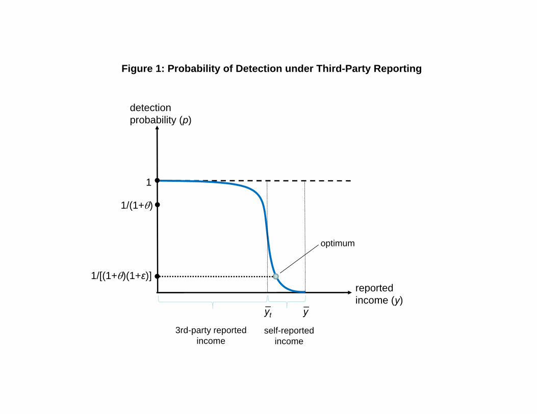
Figure 1: Probability of Detection under Third-Party Reporting

detection probability (p)probability (p)

1/(1+)

1

optimum

1/(1+)

reported1/[(1+)(1+ε)]

pincome (y)

3rd-party reported

y

self-reported

yt

income income

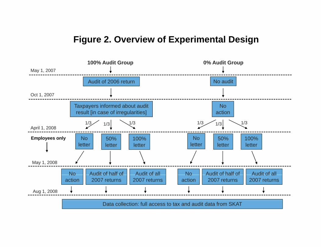
Figure 2. Overview of Experimental Design

100% Audit Group 0% Audit GroupMay 1, 2007

Audit of 2006 return No audit

Oct 1, 2007

y ,

Taxpayers informed about audit result [in case of irregularities]

Noaction

1/3 1/3 1/3 1/3 1/3 1/3

No letter

50%letter

April 1, 2008

100% letter

1/3 1/3 1/3

No letter

50%letter

100% letter

1/3 1/3 1/3

Employees only

May 1, 2008

Audit of half ofNo Audit of all Audit of half ofNo Audit of all

Aug 1, 2008

Audit of half of 2007 returns

No action

Audit of all 2007 returns

Audit of half of 2007 returns

No action

Audit of all 2007 returns

Data collection: full access to tax and audit data from SKAT

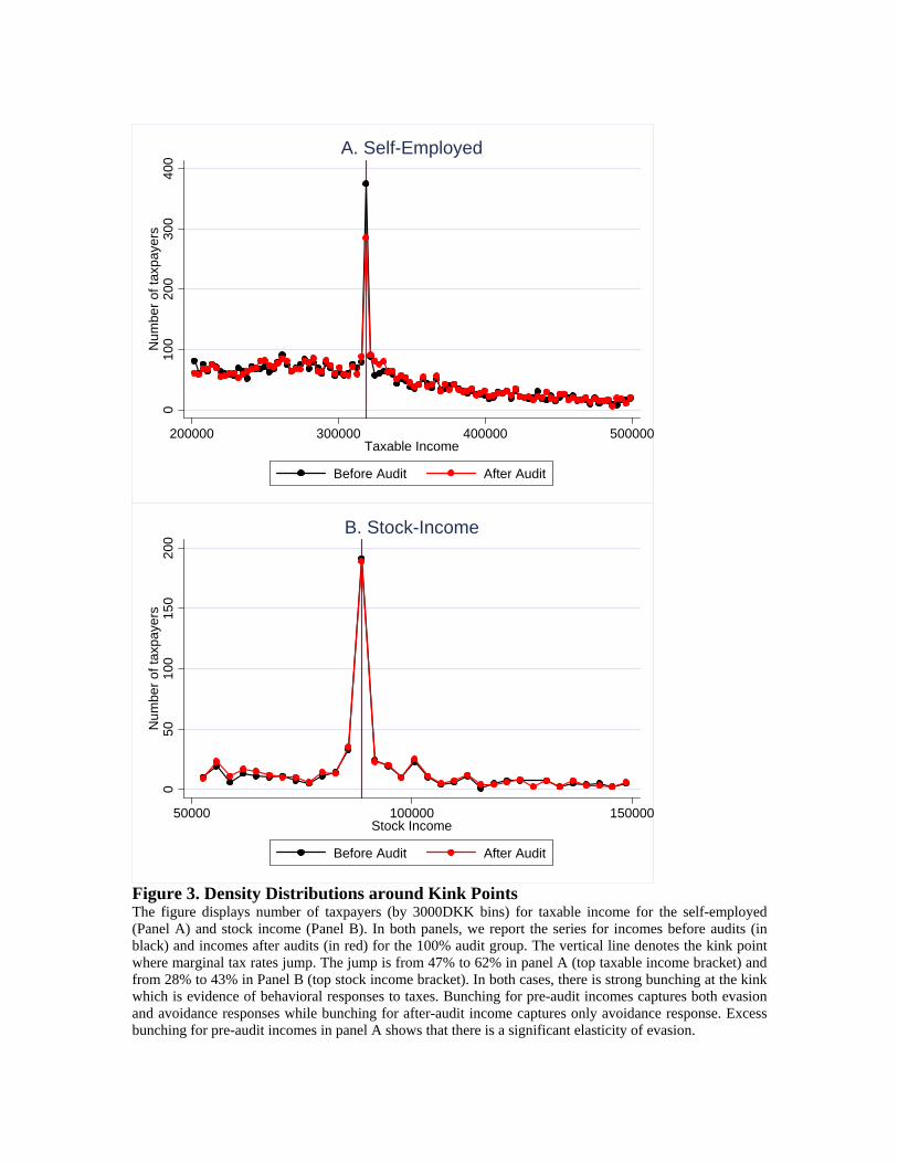
010

020

030

040

0N

umbe

r of t

axpa

yers

200000 300000 400000 500000Taxable Income

Before Audit After Audit

A. Self-Employed

050

100

150

200

Num

ber o

f tax

paye

rs

50000 100000 150000Stock Income

Before Audit After Audit

B. Stock-Income

Figure 3. Density Distributions around Kink Points The figure displays number of taxpayers (by 3000DKK bins) for taxable income for the self-employed (Panel A) and stock income (Panel B). In both panels, we report the series for incomes before audits (in black) and incomes after audits (in red) for the 100% audit group. The vertical line denotes the kink point where marginal tax rates jump. The jump is from 47% to 62% in panel A (top taxable income bracket) and from 28% to 43% in Panel B (top stock income bracket). In both cases, there is strong bunching at the kink which is evidence of behavioral responses to taxes. Bunching for pre-audit incomes captures both evasion and avoidance responses while bunching for after-audit income captures only avoidance response. Excess bunching for pre-audit incomes in panel A shows that there is a significant elasticity of evasion.

A. Income Concepts

Income Concept Definition

(1) Labor Income

(2) Personal Income

(3) Capital Income

(4) Deductions

(5) Taxable Income

(6) Stock Income

B. Tax Rates and Tax Bases

Tax Type Tax Base Bracket (DKK) Tax Rate

(1) Payroll Tax Labor Income All income 8.0%

(2) National Income Tax Personal Income + max(Capital Income,0) 38,500-265,500 5.5%265,500-318,700 11.0%

318,700- 26.5% [1]

(3) Regional Income Tax Taxable Income 38,500- 32.6% [2]

(4) Stock Income Tax Stock Income 0-44,400 28.0%44,400- 43.0%

Table 1. Danish Individual Income Tax in 2006

Notes: All amounts in Danish kroner: US $1 = 5.2 DKK as of January 2010.

Salary, wages, honoraria, fees, bonuses, fringe benefits, business earnings

Labor Income (1) + social transfers, grants, awards, gifts, received alimony - payroll tax, and certain pension contributions.Interest income, rental income, business capital income - interest on debt (mortgage, bank loans, credit cards, student loans)Commuting costs, union fees, unemployment contributions, other work related expenditures, charitable contributions, alimony paid

= Personal income (2) + Capital income (3) - Deductions (4)

Dividends and realized capital gains from corporate stock

[3]: The national and regional income taxes are based on individual income (not family income). The stock income tax is based onfamily income with brackets twice as large for married tax filers than those reported in the table.

[2]: The regional tax includes municipal and county taxes in 2006. The rate shown is the average across all municipalities, andincludes the optional church tax equal to 0.7%.

[1]: the top rate is reduced so that the combined national and regional income top marginal tax rate never exceeds 59%. The topmarginal tax rate on labor income including the payroll tax is therefore .08+.92*.59=62.3%.

Percentage share of

population

Pre-audit Income

Audit adjustment

Under-reporting

Over-reporting

Third-party income

Third-party under-

reporting

Self-reported income

Self-reported under-

reporting(1) (2) (3) (4) (5) (6) (7) (8) (9)

Net Income and Total TaxNet Income 98.4 206,038 3,744 4,255 -511 195,969 536 10,069 3,719

(0.09) (2,159) (439) (424) (132) (1,798) (80) (1,380) (416)Total Tax 90.8 69,940 1,670 1,782 -112

(0.21) (1,142) (223) (222) (21)

Positive and Negative IncomePositive Income 98.2 243,984 3,449 3,719 -271 223,882 536 20,102 3,183

(0.09) (2,511) (437) (419) (122) (1,860) (80) (1,693) (411)Negative Income 79.1 -37,946 296 536 -240 -27,913 -10,033 536

(0.29) (1,014) (73) (53) (50) (406) (862) (53)

Income ComponentsPersonal Income 95.2 209,681 2,343 2,472 -128 211,244 475 -1,563 1,997

(0.15) (1,473) (402) (401) (34) (1,385) (78) (540) (393)Capital Income 93.9 -11,075 156 335 -178 -14,556 33 3,481 302

(0.17) (340) (160) (56) (150) (602) (7) (542) (55)Deductions 60.1 -9,098 129 206 -77 -5,666 -3,432 206

(0.35) (104) (18) (16) (10) (48) (85) (16)Stock Income 22.5 5,635 274 308 -33 3,783 31 1,852 276

(0.30) (1,405) (48) (46) (12) (976) (12) (943) (45)Self-Employment 7.6 10,398 838 1,086 -248 1,164 10 9,234 1,075

(0.19) (812) (124) (130) (60) (177) (4) (816) (130)

Table 2. Audit Adjustments Decomposition

All estimates are population weighted and based solely on the 100% audit group (19,680 observations). Standard errors are reported inparenthesis.

Top panel reports net income (sum of all positive income components minus all negative income components and other deductions) and totaltax. Middle panel reports positive income (sum of all positive income components) and negative income (sum of all negative income componentsand deductions). Bottom panel displays various income components. Personal income is earnings, pensions, alimony, minus some retirementcontributions. Capital income is interest income, returns on bonds, net rents, minus all interest payments. Deductions include work relatedexpenses, union fees, charitable contributions, alimony paid, and various smaller items. Stock income includes dividends and realized capitalgains on stocks. Self-employment income is net profits from unincorporated businesses. Net income is personal income, capital income, stockincome, self-employment income, foreign income (not reported specifically), minus deductions.

Notes: Column (1) reports the percent of filers with non-zero pre-audit amounts in column (2). Columns (2) to (9) report amounts in DanishKroner (US $1 = DKK 5.2 as of 1/2010) and negative amounts are reported in negative. Column (2) displays income or tax reported beforeaudits, column (3) displays the net audit adjustment, column (4) displays under-reporting in the audit adjustment (upward audit adjustmentsincreasing tax liability), column (5) displays over-reporting in the audit adjustment (downward audit adjustments decreasing tax liability). Note that(4)+(5)=(3). Column (6) displays third-party income, column (7) displays third-party income under-reporting (defined as upward audit adjustmentsin case where third party income is higher than final reported income for positive income items), column (8) displays self-reported income(defined as total reported income minus third-party reported income), column (9) displays self-reported income under-reporting (defined allupward audit adjustments net of third-party income under-reporting). Note that (6)+(8)=(2) and (7)+(9)=(4).

B. Third-party vs. self-reported incomeA. Total income reported

Third-party income

Third-party under-

reporting

Evasion rate (2)/(1)

Amount Amount Percent

(1) (2) (3)

A. Positive Income subject to Third-Party Reporting and Withholding

All items 216,801 400 0.18(1,616) (75)

Earnings, Pensions, and Transfers 212,642 400 0.19(1,223) (75)

Other items 4,159 2 0.05=all items minus Earnings, Pensions, Transfers (978) (3)

B. Positive Income subject to Third-Party Reporting without Withholding

All items 7,081 148 2.10(769) (26)

Notes: Column (1) displays third-party income amounts, column (2) displays third-party income under-reporting (defined as upward audit adjustments in case where third party income is higher than final reported income for positive income items). Column (3) is the evasion rate defined as (2)/(1).Panel A presents results for positive income subject to both third-party reporting and tax withholding at source. It first reports total such income and then divides such income between two categories (a) earnings, pensions, and transfers (b) all other items. Panel B presents positive income subject to third-party reporting but without tax withholding at source.All estimates are population weighted. Amounts are in Danish Kroner (US $1 = 5.2 DKK). Standard errors reported in parenthesis.

Table 3. Audit Adjustments: Third-Party Reporting vs. Tax Withholding

Social factors

Socio-economic

factors

Tax return factors All factors Social

factors

Socio-economic

factors

Tax return factors All factors

(1) (2) (3) (4) (5) (6) (7) (8)

Constant 14.42 11.92 1.44 3.98 9.16 6.68 0.23 1.55(0.64) (0.66) (0.25) (0.62) (0.85) (0.95) (0.82) (1.10)

Female Dummy -5.76 -4.45 -2.05 -5.45 -3.76 -1.88(0.43) (0.45) (0.41) (0.43) (0.46) (0.43)

Married Dummy 1.55 -0.36 -1.64 -0.71 -2.13 -2.18(0.46) (0.48) (0.44) (0.49) (0.49) (0.46)

Member of church -1.98 -2.67 -1.19 -1.91 -2.48 -1.72(0.59) (0.58) (0.54) (0.59) (0.58) (0.55)

Geographical Location Copenhagen dummy -0.29 1.20 1.00 6 location p-value p-value p-value(0.67) (0.67) (0.62) dummies 0.02 0.03 1.72

Age Age>45 dummy -0.37 -0.35 0.10 4 age group p-value p-value p-value(0.45) (0.45) (0.42) dummies 0.00 0.00 17.59

Home Ownership 5.96 -0.35 3.77 -1.31(0.48) (0.46) (0.49) (0.48)

Firm Size Firm size<10 dummy 4.43 2.97 5 firm size p-value p-value(0.82) (0.76) dummies 0.00 0.00

Industrial Sector Informal sector dummy 3.25 -0.99 22 industry p-value p-value(0.86) (0.79) dummies 0.00 0.00

Self-Reported Income Dummy 9.47 9.72 7.91 8.04(0.53) (0.54) (0.56) (0.57)

(Self-Reported Income>20,000DKK) 17.46 17.08 9.51 8.56(0.91) (0.92) (1.07) (1.07)

(Self-Reported Income<-10,000DKK) 14.63 14.53 14.15 13.72(0.72) (0.72) (0.71) (0.72)

Auditing Flag Dummy 15.48 15.32 14.17 14.23(0.59) (0.60) (0.60) (0.60)

Self-Employed Dummy 12.33 10.82(0.90) (1.19)

Capital Income Dummy 0.61 1.04(0.84) (0.87)

Stock Income Dummy 1.75 2.51(0.49) (0.50)

Deduction Dummy 0.67 0.97(0.51) (0.60)

Audit Adjustment in 2004 or 2005 Dummy 9.19 8.59(0.88) (0.88)

Income controls 6 income p-value p-valuegroup dummies 0.00 0.00

R-square 1.07% 2.14% 17.14% 17.44% 2.24% 6.44% 19.16% 20.05%Adjusted R-square 1.04% 2.10% 17.13% 17.39% 2.19% 6.26% 19.10% 19.83%

Table 4. Probability of Audit Adjustments: Socio-economics vs. Tax Return Factors

Notes: This table reports coefficients of the OLS regression of an audit adjustment dummy on various dummy regressors. Bottom rows report the R-square and adjusted R-squares. Allestimates are population weighted and based solely on the 100% audit group (19,680 observations). Standard errors reported in parenthesis. In Panel A (columns (1) to (4)), we include abasic set of dummy variables, while a richer set of variables is included in Panel B (columns (5) to (8)). In Panel B, we do not report the full set of coefficients for geographical, age, firm size,industrial sector, and income groups. We instead only report the p-value from an F-test that the coefficients of those dummies are all equal to zero (for each category). The 6 locationdummies are defined as Copenhagen, North Sealand, Middle and South Sealand, South Denmark, Middle Jutland, and North Jutland. The 4 age dummies are for age groups 0-25, 26-45, 46-65, 66+. The 5 firm size dummies are for firms' size: 1, 2-10, 11-100, 101-1000, 1001+. The 6 income group dummies are for each of the bottom three quartiles separately, percentile 75 to95, percentile 95 to 99, and top percentile. For income categories, self-employed dummy means non zero self-employment income, etc.

A. Basic Variables B. Detailed Variables

Before audit income

(avoidance + evasion

elasticities)

After audit income

(avoidance elasticity only)

Difference (evasion

elasticity only)

Robustness check:

Difference using smaller sample

around kink

(1) (2) (3) (4)

A. Self-Employment Income (MTR jump from 47% to 62% at 318,700 DKK)

Fraction bunching (percent) 19.12 14.16 4.96 7.50(0.90) (0.79) (1.20) (1.85)

Elasticity 0.161 0.103 0.058 0.056(0.011) (0.009) (0.014) (0.014)

Number of observations 1,919 1,942 3,861 2,320

B. Stock Income (MTR jump from 28% to 43% at 88,600 DKK)

Fraction bunching (percent) 39.30 36.42 2.88 1.80(2.22) (2.11) (3.06) (3.69)

Elasticity 2.243 1.996 0.247 0.120(0.213) (0.191) (0.286) (0.259)

Number of observations 486 519 1,005 737

In each panel, the second row estimates the (compensated) elasticity of reported income with respect to the net-of-tax rate usingbunching evidence (following the method developed in Saez, 2009). Column (1) is the elasticity for before audit income whilecolumn (2) is the elascity for after audit income. Column (3) reports the difference between column (2) and column (1). Column(4) presents as a robustness check the difference in elasticities when the sample is limited to tax filers within 20,000 DKK(instead of 40,000 DKK) of the kink. The elasticity of before audit income combines both the evasion and avoidance elasticitieswhile the elasticity of after audit income is the tax avoidance elasticity. Therefore, the difference in elasticities is the compensatedelasticity of tax evasion with respect to the net-of-tax rate.

In each panel, the first row estimates the fraction of tax filers bunching (income within 1500 DKK of the kink) among tax filers withincome within 40,000 DKK of the kink. Column (1) is for income before audit while column (2) is for income after audit. Column(3) reports the difference between column (1) and column (2). Column (4) presents a robustness check the difference when thesample is limited to tax filers within 20,000 DKK (instead of 40,000 DKK) of the kink.

Table 5. Tax Evasion vs. Tax Avoidance ElasticitiesBaseline Differences

Notes: This table estimates the effects of marginal tax rates on tax evasion vs. tax avoidance using bunching evidence aroundkink points of the tax schedule where marginal tax rates jump. Panel A focuses on the self-employed and the top rate kink wheremarginal tax rates jump from 47% to 62% at 318,700 DKK. Panel B focuses on stock-income and the top rate kink for stock-income where marginal tax rates from 28 to 43% at 88,600 DKK for married filers and 44,300 DKK for single filers (we havealigned single filers by multiplying by two their stock income). As shown in Figure 2, in both cases, there is significant evidence ofbunching at the kink both for income before audits and incomes after audits.

0% audit group

100% audit group

Difference 100%-0%

Difference standard

error

No Letter group

Letter group

Difference (5)-(6)

Difference standard

error(1) (2) (3) (4) (5) (6) (7) (8)

Net Income 265,069 263,485 -1,584 (5,996) 239,858 244,559 4,701 (3,415)Total Tax 100,909 100,460 -449 (2,991) 82,444 84,245 1,801 (1,583)Personal Income 216,048 216,993 946 (2,345) 255,923 258,842 2,918 (2,887)Capital Income -13,132 -12,805 327 (1,015) -16,647 -15,439 1,208 (532)Deductions -11,838 -11,976 -138 (160) -8,364 -8,287 76 (159)Stock Income 17,998 15,880 -2,118 (4,869) 7,656 8,101 445 (1,778)Self-Employment 55,616 54,960 -656 (2,869)Female (%) 39.93 39.59 -0.33 (0.47) 49.82 50.10 0.28 (0.67)Age 49.28 49.43 0.14 (0.16) 49.10 48.90 -0.20 (0.25)

% with Net Income 99.55 99.52 -0.03 (0.07) 98.70 98.65 -0.05 (0.15)% with Total Tax 96.72 96.61 -0.11 (0.17) 96.61 96.27 -0.34 (0.25)% with Personal Income 94.87 94.73 -0.14 (0.21) 97.19 97.04 -0.15 (0.23)% with Capital Income 95.67 95.40 -0.27 (0.20) 96.97 96.92 -0.05 (0.23)% with Deductions 71.68 71.76 0.07 (0.44) 64.22 64.48 0.26 (0.64)% with Stock Income 40.30 40.23 -0.07 (0.47) 44.15 43.59 -0.56 (0.67)% with Self-Employment 40.18 40.37 0.19 (0.47)

Number of observations 23,148 19,630 42,778 9,449 15,339 24,788

In panel B, the sample is restricted to tax filers with no self-employment in base year as the letter experiment was limited to taxfilers with no self-employment income. Estimates are weighted according to the experiment stratification design. Weights do notreflect population weights. All the amounts are in Danish Kroner (US $1 = DKK 5.2 as of 1/2010).

Table 6. Randomization Checks: Audit and Letter experimentsA. Audit randomization B. Letter Randomization

Notes: This table presents randomization checks for the audit experiment (panel A, cols. (1) to (4)) and the letter experiment(panel B, cols. (5) to (8)). Panel A compares baseline reported incomes in 2006 (before the audit experiment took place). Columns(1) and (2) present the baseline averages for the treatment group and control group respectively. Column (3) presents thedifference between the treatment group and the control group. The standard error of the difference is presented in column (4).Panel B compares pre-populated tax returns for 2007 incomes before the letters are sent. The columns are constructed as inPanel A.

Baseline

Audit adjustment in 100% audit group

Increase in 0% audit group

Difference 100% audit vs. 0% audit

Increase in 0% audit group

Difference 100% audit vs. 0% audit

Increase in 0% audit group

Difference 100% audit vs. 0% audit

(1) (2) (3) (4) (5) (6) (7)

A. Probability of Income Increase from 2006 to 2007 (percent)

Net Income 21.95 60.84 0.90 37.47 2.11 59.30 0.24(0.30) (0.33) (0.48) (0.32) (0.48) (0.33) (0.48)

Total Tax 21.41 56.14 0.99(0.29) (0.33) (0.49)

Personal Income 2.84 63.74 0.29 11.24 0.41 63.55 0.38(0.12) (0.32) (0.47) (0.21) (0.31) (0.32) (0.47)

Capital Income 4.24 44.55 -0.03 22.24 0.39 43.45 0.18(0.14) (0.33) (0.49) (0.28) (0.41) (0.33) (0.49)

Deductions 4.43 27.87 0.69 17.46 0.93 20.14 0.15(0.15) (0.30) (0.44) (0.25) (0.38) (0.27) (0.39)

Stock Income 1.64 23.67 0.53 5.44 0.19 23.24 0.39(0.09) (0.28) (0.42) (0.15) (0.22) (0.28) (0.42)

Self-Employment 14.49 20.19 1.62 20.20 1.53 3.46 0.13(0.25) (0.27) (0.40) (0.27) (0.40) (0.12) (0.18)

B. Amount of Income Change from 2006 to 2007

Net Income 5629 4444 2554 1696 2322 2748 232(497) (536) (787) (448) (658) (467) (691)

Total Tax 2510 2013 1377(165) (319) (464)

Personal Income 592 7207 168 -442 -144 7649 313(147) (435) (638) (190) (277) (410) (604)

Capital Income 145 -3616 68 2575 -47 -6191 114(456) (185) (275) (207) (306) (202) (299)

Deductions 102 205 167 -145 107 350 60(23) (70) (101) (70) (101) (23) (33)

Stock Income 485 805 508 -88 633 893 -125(71) (202) (293) (165) (237) (133) (195)

Self-Employment 4287 71 1745 587 1804 -516 -59(286) (387) (571) (390) (579) (135) (204)

For panel B, all the amounts are in Danish Kroner (US $1 = DKK 5.2 as of 1/2010). Income changes are trimmed at -200,000 DKK and 200,000 DKK. That is, income changes are defined asmin(200000,max(income in 2007-income in 2006,-200000). This is done to avoid extreme outcomes which make estimates very imprecise. Less than 2% of observations are trimmed on average.

All income items are estimated for the full sample (40,602 observations). Estimates are weighted according to the experiment stratification design. Weights do not reflect population weights. Standarderrors are reported in parenthesis.

Table 7. Effects of Prior Audits on Year to Year Income Changes

Notes: This table reports the effects of prior-audits on income changes from 2006 to 2007. Panel A focuses on the probability of a (nominal) income increase while Panel B focuses on the amounts ofincome changes. Column (1) reports the fraction with an audit adjustment in the 100% audit group in base year (Panel A) and the average amount of the audit adjustment in base year (Panel B). Columns(2) reports the fraction with an income increase from 2006 to 2007 (Panel A) or the average income increase from 2006 to 2007 (Panel B) for the 0% audit group. Column (3) reports the difference betweenthe 100% audit group and the 0% audit group in the fraction with an income increase from 2006 to 2007 (Panel A) or the average income increase from 2006 to 2007 (Panel B). Each row corresponds to agiven income items. The complete definition of each income item is given in Table 2. Columns (4)-(5) repeat the analysis of cols. (2)-(3) limited to self-reported incomes instead of total reported income.Columns (6)-(7) repeat the analysis limited to third-party reported incomes instead of total reported income.

Total Income Change Self-Reported Income Change Third-Party Reported Income Change

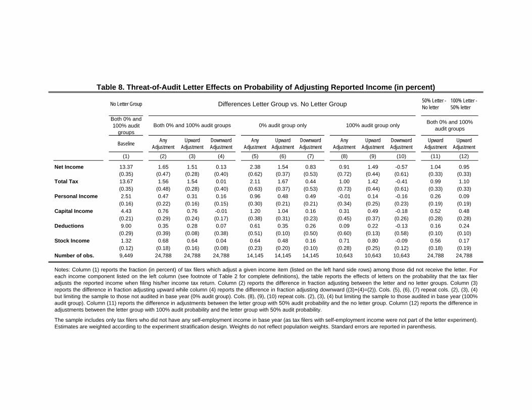
No Letter Group 50% Letter - No letter

100% Letter - 50% letter

Both 0% and 100% audit

groups

Baseline Any Adjustment

Upward Adjustment

Downward Adjustment

Any Adjustment

Upward Adjustment

Downward Adjustment

Any Adjustment

Upward Adjustment

Downward Adjustment

Upward Adjustment

Upward Adjustment

(1) (2) (3) (4) (5) (6) (7) (8) (9) (10) (11) (12)

Net Income 13.37 1.65 1.51 0.13 2.38 1.54 0.83 0.91 1.49 -0.57 1.04 0.95(0.35) (0.47) (0.28) (0.40) (0.62) (0.37) (0.53) (0.72) (0.44) (0.61) (0.33) (0.33)

Total Tax 13.67 1.56 1.54 0.01 2.11 1.67 0.44 1.00 1.42 -0.41 0.99 1.10(0.35) (0.48) (0.28) (0.40) (0.63) (0.37) (0.53) (0.73) (0.44) (0.61) (0.33) (0.33)

Personal Income 2.51 0.47 0.31 0.16 0.96 0.48 0.49 -0.01 0.14 -0.16 0.26 0.09(0.16) (0.22) (0.16) (0.15) (0.30) (0.21) (0.21) (0.34) (0.25) (0.23) (0.19) (0.19)

Capital Income 4.43 0.76 0.76 -0.01 1.20 1.04 0.16 0.31 0.49 -0.18 0.52 0.48(0.21) (0.29) (0.24) (0.17) (0.38) (0.31) (0.23) (0.45) (0.37) (0.26) (0.28) (0.28)

Deductions 9.00 0.35 0.28 0.07 0.61 0.35 0.26 0.09 0.22 -0.13 0.16 0.24(0.29) (0.39) (0.08) (0.38) (0.51) (0.10) (0.50) (0.60) (0.13) (0.58) (0.10) (0.10)

Stock Income 1.32 0.68 0.64 0.04 0.64 0.48 0.16 0.71 0.80 -0.09 0.56 0.17(0.12) (0.18) (0.16) (0.08) (0.23) (0.20) (0.10) (0.28) (0.25) (0.12) (0.18) (0.19)

Number of obs. 9,449 24,788 24,788 24,788 14,145 14,145 14,145 10,643 10,643 10,643 24,788 24,788

The sample includes only tax filers who did not have any self-employment income in base year (as tax filers with self-employment income were not part of the letter experiment).Estimates are weighted according to the experiment stratification design. Weights do not reflect population weights. Standard errors are reported in parenthesis.

Table 8. Threat-of-Audit Letter Effects on Probability of Adjusting Reported Income (in percent)

Notes: Column (1) reports the fraction (in percent) of tax filers which adjust a given income item (listed on the left hand side rows) among those did not receive the letter. Foreach income component listed on the left column (see footnote of Table 2 for complete definitions), the table reports the effects of letters on the probability that the tax fileradjusts the reported income when filing his/her income tax return. Column (2) reports the difference in fraction adjusting between the letter and no letter groups. Column (3)reports the difference in fraction adjusting upward while column (4) reports the difference in fraction adjusting downward ((3)+(4)=(2)). Cols. (5), (6), (7) repeat cols. (2), (3), (4)but limiting the sample to those not audited in base year (0% audit group). Cols. (8), (9), (10) repeat cols. (2), (3), (4) but limiting the sample to those audited in base year (100%audit group). Column (11) reports the difference in adjustments between the letter group with 50% audit probability and the no letter group. Column (12) reports the difference inadjustments between the letter group with 100% audit probability and the letter group with 50% audit probability.

Both 0% and 100% audit groups 0% audit group only

Differences Letter Group vs. No Letter Group

100% audit group only Both 0% and 100% audit groups