NASA TECHNICAL NOTE N A S A T_N --D-5722 9. 1

N N h m I

n z c e r/)e z

A STUDY OF RADIATION HEAT TRANSFER FROM A CYLINDRICAL FIN WITH BASE SURFACE INTERACTION

by Churles A. Cothrun

George C. MurshaZZ Space Flight Center Marshall, Ah .

E"3 z

N A T I O N A L A E R O N A U T I C S A N D S P A C E A D M I N I S T R A T I O N W A S H I N G T O N , D. C. A P R I L 1970 I

1 yi

..-

L

https://ntrs.nasa.gov/search.jsp?R=19700014952 2020-04-15T23:41:20+00:00Z

TECH LIBRARY KAFB, NM

I11111111111lllll111111111llllllllllIll1Ill1 0 I3 L5 3.8

1. REPORT NO. 2. GOVERNMENT ACCESSION NO. 3. RECIPIENT'S CATALOG NO. I

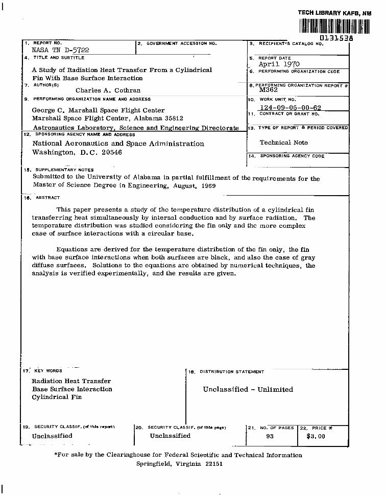
NASA TN D-5722 4. T I T L E AND SUBTITLE 5. REPORT DATE

A p r i l 1970 A Study of Radiation Heat Transfer From a Cylindrical 6. PERFORMING ORGANIZATION CODE

Fin With Base Surface Interaction ~

7. AUTHOR(S) 8. PERFORMING ORGANIZATION REPORT j

Charles A. Cothran M362 ~~

9. PERFORMING ORGANIZATION NAME AND ADDRESS IO. WORK UNIT, NO,

124-09-05-00-62George C. Marshall Space Flight Center 11. CONTRACT OR GRANT NO.Marshall Space Flight Center, Alabama 35812 Astronautics Laboratory, Science and Engineering Directorate 13. T Y P E OF REPORT & PERIOD COVEREI

12. SPONSORING AGENCY NAME AND ADDRESS

National Aeronautics and Space Administration Technical Note Washington, D. C. 20546 1.1. SPONSORING AGENCY CODE

.- . .

15. SUPPLEMENTARY NOTES

Submitted to the University of Alabama in partial fulfillment of the requirements for the Master of Science Degree in Engineering, August, 1969

Is, -ABSTRACT

This paper presents a study of the temperature distribution of a cylindrical f in transferring heat simultaneously by internal conduction and by surface radiation. The temperature distribution was studied considering the fin only and the more complex case of surface interactions with a circular base.

Equations are derived for the temperature distribution of the fin only, the fin with base surface interactions when both surfaces are black, and also the case of gray diffuse surfaces. Solutions to the equations are obtained by numerical techniques, the analysis is verified experimentally, and the results are given.

~

7.' KEY WORDS 18. DISTRIBUTION STATEMENT

Radiation Heat Transfer Base Surface Interaction Unclassified - Unlimited Cylindrical Fin

9. SECURITY CLASSIF. (of thh ropmt) 20. SECURITY CLASSIF. (of thh p e e ) 21. NO. OF PAGES 22. PRICE JC

Unclassified Unclassified I 93 $3.00

~~~~. -

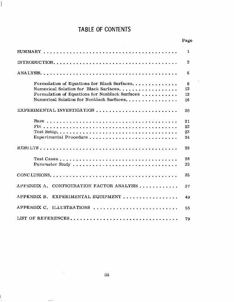
TABLE OF CONTENTS

Page

SUMMARY ......................................... I

INTRODUCTION...................................... 2

ANALYSIS.......................................... 6

Formulation of Equations for Black Surfaces.............. 6 Numerical Solution f o r Black Surfaces.................. 13 Formulation of Equations for Nonblack Surfaces ........... 13 Numerical Solution for Nonblack Surfaces ................ -16

EXPERIMENTAL INVESTIGATION ......................... 20

Base ........................................ 21 Fin ......................................... 22 TestSetup..................................... 23 Experimental Procedure ........................... 24

RESULTS .......................................... 28

T e s t c a s e s .................................... 28 Parameter Study ................................ 33

CONCLUSIONS....................................... 35

APPENDIX A . CONFIGURATION FACTOR ANALYSIS . . . . . . . . . . . . 37

APPENDIX B . EXPERIMENTAL EQUIPMENT . . . . . . . . . . . . . . . . . 49

APPENDIX C. ILLUSTRATIONS .......................... 55

LISTOFREFERENCES ................................. 79

iii

Figure

I . 2 .

A-I .

A.2 .

c.1 . c.2 .

c.3 .

c.4 .

c.5 .

C.6 .

c.7 .

C.8 .

c.9 .

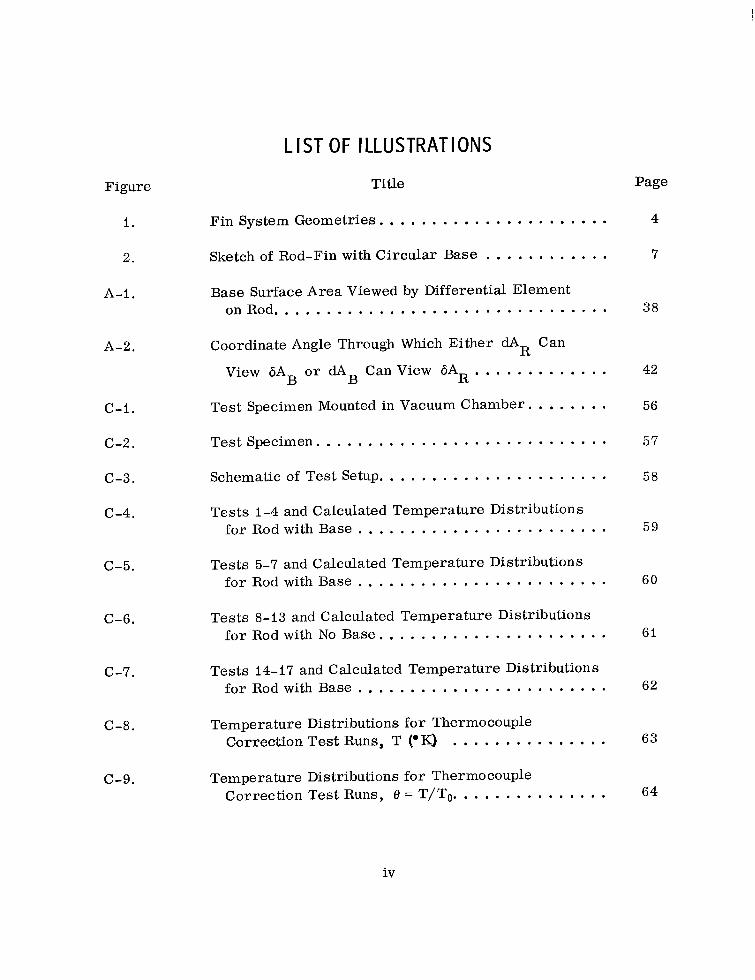
L IST OF ILLUSTRATIONS

Title

Fin System Geometries ...................... Sketch of Rod-Fin with Circular Base . . . . . . . . . . . . Base Surface Area Viewed by Differential Element

onRod . . . . . . . . . . . . . . . . . . . . . . . . . . . . . . . . Coordinate Angle Through Which Either dAR Can

View 6AB o r dAB CanView 6AR . . . . . . . . . . . . . Test Specimen Mounted in Vacuum Chamber . . . . . . . . Test Specimen . . . . . . . . . . . . . . . . . . . . . . . . . . . . Schematic of Test Setup. . . . . . . . . . . . . . . . . . . . . . Tests 1-4 and Calculated Temperature Distributions

fo r Rod with Base . . . . . . . . . . . . . . . . . . . . . . . . Tests 5-7 and Calculated Temperature Distributions

for Rod with Base . . . . . . . . . . . . . . . . . . . . . . . . Tests 8-13 and Calculated Temperature Distributions

f o r Rod with No Base ...................... Tests 14-17 and Calculated Temperature Distributions

for Rod with Base ........................ Temperature Distributions for Thermocouple

Correction Test Runs. T CK) . . . . . . . . . . . . . . . Temperature Distributions fo r Thermocouple

Correction Test Runs. 8 = T/T0. . . . . . . . . . . . . . .

Page

4

7

38

42

56

57

58

59

60

61

62

63

64

iv

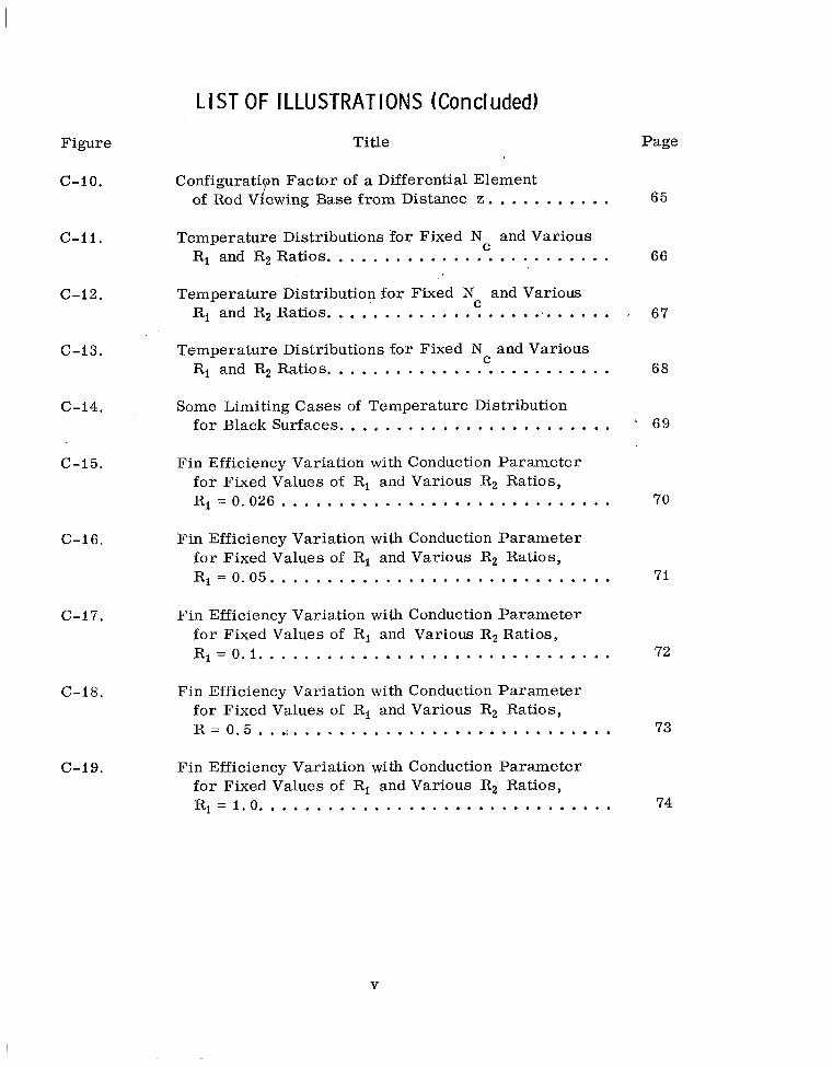
L I S T OF ILLUSTRATIONS (Concluded) Figure Title Page

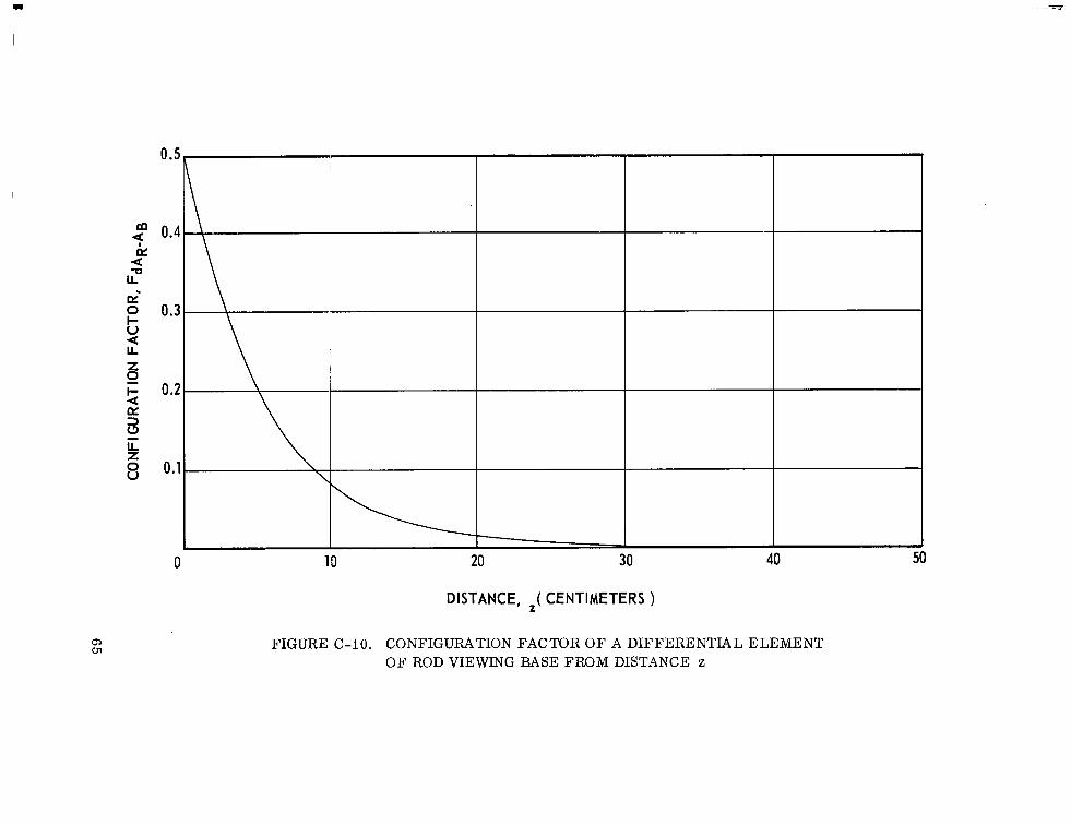
c-io. Configurati n Factor of a Differential Element of Rod VPewing Base f rom Distance z . . . . . . . . . . . 65

c-11. Temperature Distributions 'for Fixed N and Various CR, and R 2 R a t i o s . . ....................... 66

c-12. Temperature Distribution fo r Fixed N and Various C

R, and R2 Ratios. .......................... 67

C-13. Temperature Distributions for Fixed N and Various R, and R2 Ratios. ........................ 68

C-14. Some Limiting Cases of Temperature Distribution fo r Black Surfaces. ....................... ' 69

C-15. Fin Efficiency Variation with Conduction Parameter f o r Fixed Values of R, and Various R2 Ratios, R, = 0 . 0 2 6 . . . . . . . . . . . . . . . . . . . . . . . . . . . . . 70

C-16. Fin Efficiency Variation with Conduction Parameter f o r Fixed Values of R, and Various R2 Ratios, R l = 0 . 0 5 . . . . . . . . . . . . . . . . . . . . . . . . . . . . . . 71

C-17. Fin Efficiency Variation with Conduction Parameter fo r Fixed Values of R, and Various R2 Ratios, R , = O . I . . . . . . . . . . . . . . . . . . . . . . . . . . . . . . . 72

C-18. Fin Efficiency Variation with Conduction Parameter fo r Fixed Values of R, and Various R2 Ratios, R = 0 . 5 . . . 1 . . . ......................... 73

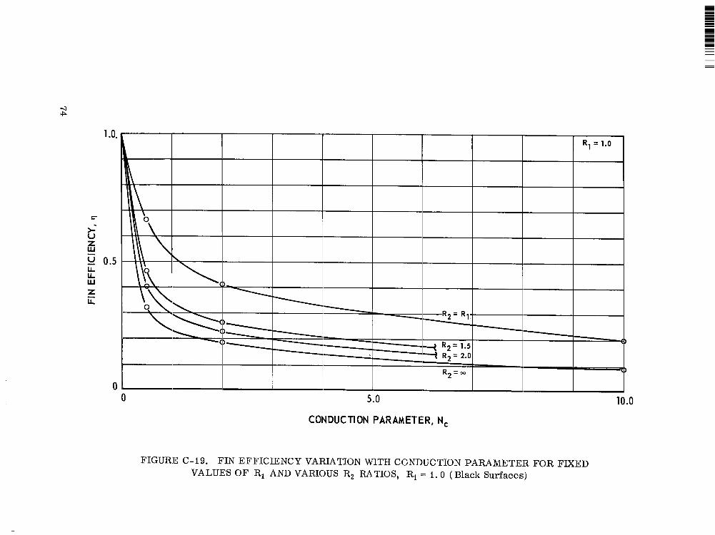
c-19. Fin Efficiency Variation with Conduction Parameter for Fixed Values of R, and Various R2 Ratios, R l = 1 . 0 . . . . . . . . . . . . . . . . . . . . . . . . . . . . . . . 74

C

V

Table

C-1.

c-2.

c-3.

c-4.

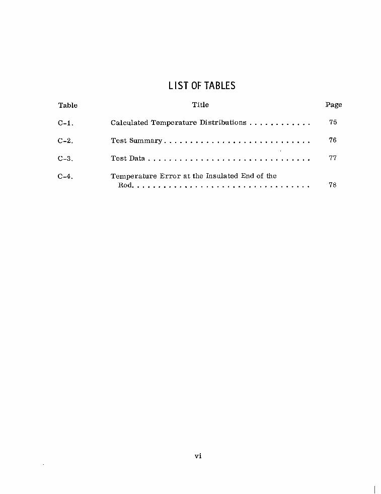
L I S T OF TABLES

Title Page

Calculated Temperature Distributions . . . . . . . . . . . . 75

Test Summary. . . . . . . . . . . . . . . . . . . . . . . . . . . . 76

Tes t Da ta . . . . . . . . . . . . . . . . . . . . . . . . . . . . . . . 77

Temperature E r r o r a t the Insulated End of the Rod. . . . . . . . . . . . . . . . . . . . . . . . . . . . . . . . . . 78

vi

NOMENCLATURE A

A'

B

B*

F

k

L

M

N C

N

N'

A n

A r e a (cm2 or ft2)

That portion of a la rger a rea that is viewed from a specified location (cm2 o r ft2)

Area with differential width and finite length

Radiosity (W/cm2 o r Btu/ftf-hr)

Radiosity (dimensionless)

Differential

Configuration factor (dimensionless)

Configuration factor in te rms of dimensionless parameters

Irradiation from surroundings (W/cm2 o r Btu/ft2-hr)

Irradiation from the system (W/cm2 o r Btu/ft2-hr)

Irradiation f rom the system (dimensionless)

Unit vectors

Thermal conductivity (W/cm-O K o r Btu/ft-hr-O R)

Direction cosines

Length (cm)

Number of isothermal segments of the specimen

Conduction parameter (dimensionless)

N Ec R

Unit vector normal to a surface

vii

r

-S

A S

S

T

X

XYY, z

Z

a!

6.. 13

E

rl

e

71

P

P'

0

T,T'

NOMENCLATURE (Cont inued

Rate of heat flow (W)

Dimensionless ratio, r/L

Radius (cm)

Line

Vector

Magnitude of line s Absolute temperature (degrees Kelvin, e K)

Rectangular coordinates

Dimensionless ratio, z/L

Absorptivity (dimensionless )

Kronecker delta

Emissivity (dimensionless)

Efficiency (dimensionless)

Dimensionless temperature , T/To

3.14159

Cylindrical radius coordinate

Reflectivity (dimensionless)

Stefan-Boltzmann constant (5.6699 x lo-" W/cm2-"K4 o r 0.1713 x Btu/ft2-hr-.R4)

Dummy integration variables

viii

NOMENCLATURE (Concluded)

cp Cylindrical coordinate angle

$ Inverse of X

Subscripts :

B Base surface

i, j i denotes a specific element of j elements

R Rod surface

6A Differential s t r ip a rea

dA Differential a rea

0 , 1 , 2 . . 1 1 Thermocouple station locations on the rod tes t specimen

ACKNOWLEDGMENT

The author would like to take this opportunity to acknowledge the

contributions of those persons whose assistance was most prominent in the

preparation of this thesis. Sincere thanks are extended to Dr. A. R. Shouman

for his many helpful comments and for his efforts in sponsoring the use of the

MSFC Propulsion and Vehicle Engineering Laboratory test equipment and

facilities. Sincere thanks are also extended to Dr. R. Blanton, his thesis

advisor, for h is many helpful comments and his guidance and to Miss Lucy

Coward of the MSFC Computation Laboratory who programmed the numerical

solutions of the temperature distribution equations,

X

A STUDY OF RADIATION HEAT TRANSFER FROM A CYLINDRICAL FIN WITH BASE SURFACE

INTERACT ION

SUMMARY

In this study the temperature distribution and heat t ransfer rates of a

cylindrical radiating fin w e r e investigated, considering no base surface inter­

action and also the case of interaction with a circular base. Surroundings of

the fin were assumed to be black and at a temperature of absolute zero.

The equations governing the temperature distribution of a fin attached

to a circular base causing radiation interaction were derived for two cases: I 1

when their surfaces were black; and when their surfaces were gray and diffuse.

Solutions to the equations w e r e obtained by numerical techniques and the

analysis w a s qualitatively verified with experimental studies.

Numerical solutions were obtained for the specific conditions of each

of the 20 tes t runs and for a wide variation of the governing parameters for a

black rod and base. The parameter study showed that the rod heat t ransfer

efficiency may vary as much as 50% with changing base size. The experimental

data and numerical solutions showed trend agreement. However, it w a s shown

that substantial e r r o r in the measured temperature distribution could be

attributed to the use of an excessive number of thermocouples and the carbon

coating used during ten of the tests.

INTRODUCTION

The subject of heat transfer f rom fins and extended surfaces has been .

studied analytically and experimentally for almost two centuries [ I ] . Until

recent years most work w a s concentrated on convection f rom fins with constant

thermal properties. The problem of a fin exchanging heat with i t s surround­

ings by radiation has only recently come under extensive study as a result of

man's interest in space and the newly found capability fo r space travel,

The temperature distribution along a thin rod, wi re , o r thin-walled

tube heated by an electric current while in a vacuum has been of interest ,

both experimentally and theoretically, for a long time. The l i terature on this

problem contains work by Langmuir [ 2 ] , Langmuir and Taylor [3 ] , Worthing

[4], Worthing and Holliday [ 51 , Stead [ 61 , Bush and Gould [7] , Baerwald [ 81 ,

Jain and Krishman [91 , and Shouman [ IOJ . Shouman [IO] presented an exact

solution fo r a one-dimensional fin with constant c ros s sectional area and

constant thermal properties that transferred heat from its surface by radiation

only to an equivalent sink temperature.

The interest in space exploration generated an interest in fins of

various geometries applicable to heat exchanger designs. The ear ly

published work in this a r e a treated the temperature distribution of isolated

fins, Lieblien [ 111 analyzed the temperature distribution along a rectangular

fin and Chambers and Somers [I21 presented a s imilar analysis of a circular

2

fin. Tatom [ 131 presented the mathematical formulation f o r the temperature

distribution along a rod and presented an exact solution fo r the special case

of an infinitely long rod.

The analysis of fins then proceeded to the consideration of mutual

irradiation of fins and their base surfaces. ' Callinan and Berggren [ 141 con­

sidered a wide range of design problems and'studied the fin geometry shown

in Figure IA; however, the base surface effect and.multiple reflections were

not considered. Bartas and Sellers [ 151 indicated the importance of radiation

interaction f o r this design and considered a singly reflected ray in the analytical

formulation but omitted the singly reflected ray fo r the solutions presented.

The problem of flat rectangular fins sharing a common edge, Figure

IB, w a s studied by Sparrow, Eckert, and Irvine [ 161. These authors formu­

lated the solutions f o r this geometry, and in another study [ 171, they presented

solutions for mutual irradiation between fins whose surfaces are gray and

reflect diffusely. A similar arrangement, but of trapezoidal c r o s s section,

w a s considered by Karlekar and Chao [ 181; they presented an optimization

procedure for achieving maximum dissipation. Hering [ 191 studied this fin

system and presented solutions f o r gray surfaces which reflect specularly,

and he compared the effectiveness of the cases of specular and diffuse

reflections.

3

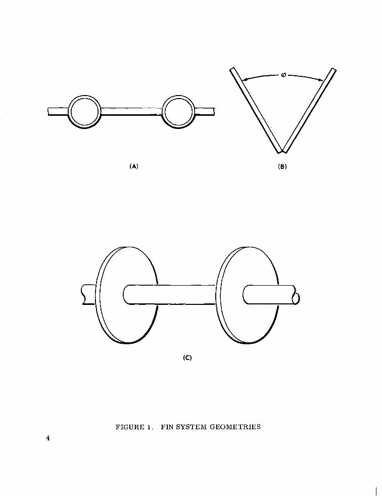
FIGURE I.FIN SYSTEM GEOMETRIES 4

A complete mathematical formulation of the governing equations fo r the

system shown in Figure i A w a s presented by Sparrow and Eckert [20] . They

considered the mutual irradiation between the fin and base surfaces and

irradiation f rom external sources . The case of selective gray surfaces w a s

also considered. However, the solutions presented w e r e fo r black surfaces

with negligible irradiation f rom external sources . The physical parameters

were varied over a wide range and the conduction parameter , Nc, was varied

from 0. 5 to 20. Sarabia and Hitchcock [ 2 i ] presented the solutions for this

system in te rms of overall fin-tube efficiency for the black and gray diffuse

cases. The conduction parameter w a s varied from i to 20 for the black case

and the data were presented for N = Ifor the gray diffuse case. Hwang-BoC

[ 221 also considered this sytem and presented a method of maximizing heat

rejection per unit weight; however, irradiation was simplified by neglecting

components reflected twice o r more.

Sparrow, Miller and Jonsson [23] studied the fin system shown in

Figure 1C with gray diffuse surfaces. The system consisted of annular fins

mounted on a constant temperature tube with mutual irradiation between the

fins and the tube. The problem w a s solved for a wide range of physical

parameters , and the conduction parameter w a s varied from 0 to 0.7.

The effects of convection were considered negligible in the previously

mentioned papers and were neglected fo r this study. Gordon [ 241 substantiated

that convection w a s negligible at p re s su res below mil l imeters of mercury.

5

The mathematical formulation of the energy balance on a differential

element of a fin t ransferr ing heat by internal conduction and by surface

radiation resu l t s in a second order nonlinear differential equation. The

equation is fur ther complicated when the mutual irradiation by the fin base

surface, other fins, and external sources are considered. A s a result of these

complications, an exact solution is not known and numerical techniques must

be employed. An exact solution for a fin not considering interaction with other

surfaces has been published by Shouman [ I O ] . In a t e s t program to verify

his solution f o r the temperature distribution of a fin, Shouman used an

1aluminum rod 2. 54 c m (I inch) in diameter and 48. 90 cm (19-4 inches) long.

A s an extension of this work i t was decided to investigate, both analytically and

experimentally, the effect of adding a base surface upon the temperature

distribution of the radiating rod.

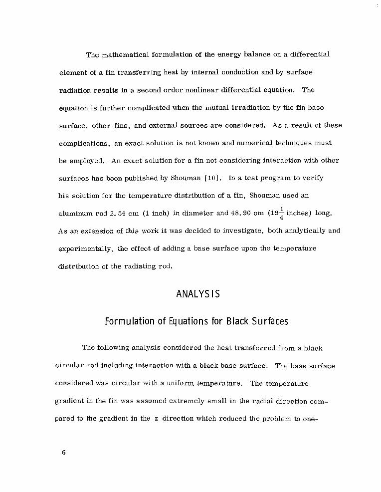
ANALYSIS

Formulation of Equations for Black Surfaces

The following analysis considered the heat t ransferred from a black

circular rod including interaction with a black base surface. The base surface

considered was c i rcular with a uniform temperature. The temperature

gradient in the fin w a s assumed extremely small in the radial direction com­

pared to the gradient in the z direction which reduced the problem to one­

6

In addition, the following assumptions w e r edimensional heat flow in the rod.

made:

1.

2.

3.

4.

The rod was isotropic and homogeneous.

The material thermal properties w e r e constant.

There were no heat sources or sinks in the rod.

The system and surroundings w e r e a t thermal equilibrium.

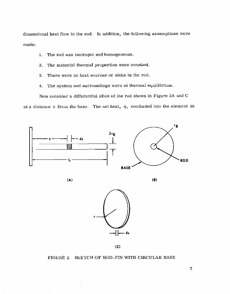
Now consider a differential slice of the rod shown in Figure 2A and C

a t a distance z f rom the base. The net heat, q , conducted into the element dz

T BASE

FIGURE 2. SKETCH OF ROD-FIN WITH CIRCULAR BASE

7

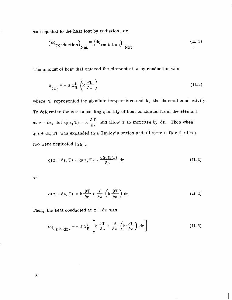
was equated to the heat lost by radiation, or

(dqconduction)Net = (dqradiation) Net (11-1)

The amount of heat that entered the element at z by conduction w a s

(11-2)

where T represented the absolute temperature and k, the thermal conductivity.

To determine the corresponding quantity of heat conducted from the element

at z + dz, let q ( z , T ) = k -a T and allow z to increase by dz. Then when az

q( z + dz, T) was expanded in a Taylor's s e r i e s and all t e rms after the first

two were neglected [ 2 5 ] ,

o r

aT -a ( k E ) dzq ( z -f dz ,T) = k-+ az az

Then, the heat conducted a t z + dz w a s

- - 7rr2 dz]dq( z -c dz) - R [kE+5(k5)

(11-3)

(11-4)

(11-5)

8

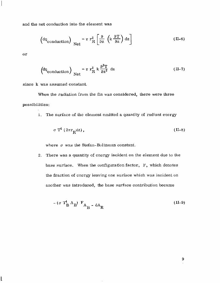
and the net conduction into the element was

(dqconduction ) N e t = 7~ rk [& 6%) dz] (11-6)

or

- 2 a2T (%onduction) Net - 7r rR 3 dz

(11-7)

since k w a s assumed constant.

When the radiation f rom the fin w a s considered, there were three

possibilities:

I.The surface of the element emitted a quantity of radiant energy

CJ ? ( 2arRdz) , (11-8)

where IT w a s the Stefan-Boltzman constant.

2. There w a s a quantity of energy incident on the element due to the

base surface. When the configuration factor, F, which denotes

the fraction of energy leaving one surface which was incident on

another was introduced, the base surface contribution became

( 11-9)

9

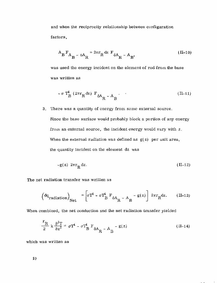
and when the reciprocity relationship between configuration

factors,

A F = 2nrRdz FB AB - MR 6AR - AB’

(11-IO)

w a s used the energy incident on the element of rod f rom the base

w a s written as

- CJ l!jB( 2rrRdz) F MR - AB (11-1 1 )

3 . There w a s a quantity of energy from some external source.

Since the base surface would probably block a portion of any energy

from an external source, the incident energy would vary with z.

When the external radiation w a s defined as g( z) pe r unit a rea ,

the quantity incident on the element dz w a s

-g(z) 2nrR dz. (11-12)

The net radiation t ransfer was written as

- g(z)] 2xrRdz. (11-13) B

When combined, the net conduction and the net radiation transfer yielded

( 11- 14)

which w a s written as

10

--

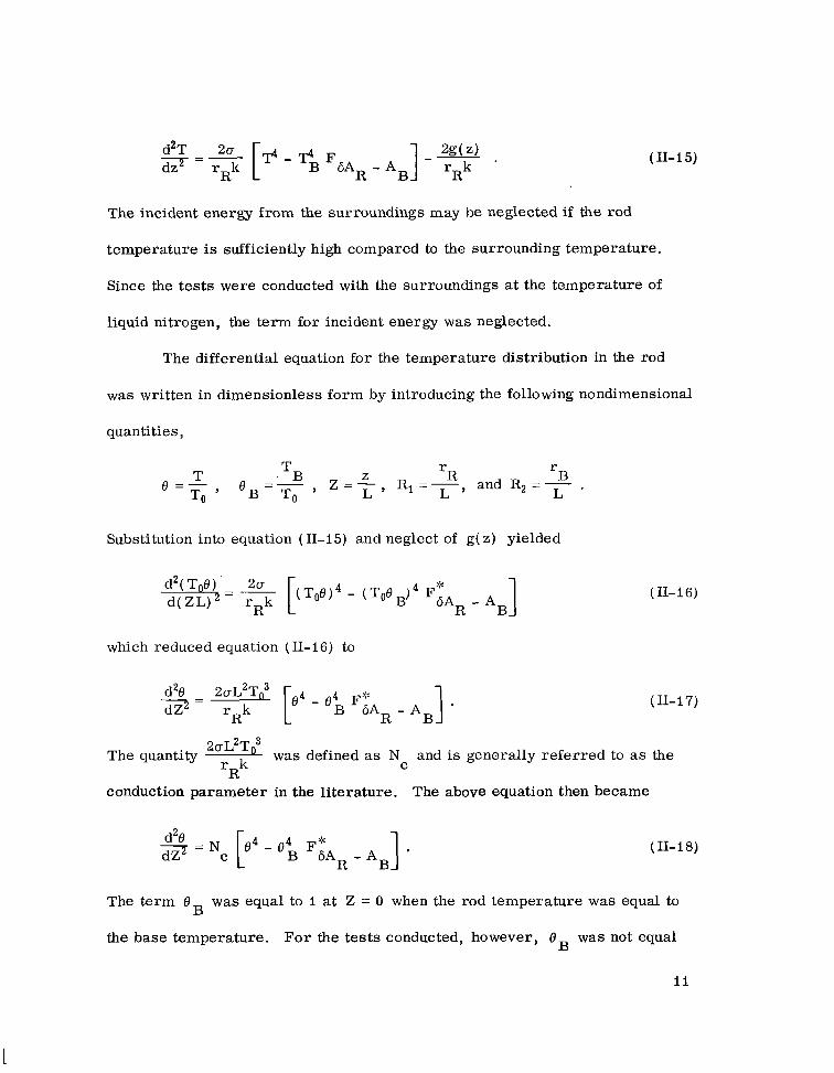
d2Ts=­2o [Td - TdB FdAR- *B (11-15)

rRk

The incident energy from the surroundings may be neglected if the rod

temperature is sufficiently high compared to the surrounding temperature.

Since the tests were conducted with the surroundings at the temperature of

liquid nitrogen, the term for incident energy w a s neglected.

The differential equation for the temperature distribution in the rod

was written in dimensionless form by introducing the following nondimensional

quantities,

r r e =-T . TB

' z = -Z

L ' R, =

R , and R2= B .

T o ' ' B - T 0

Substitution into equation (11-15) and neglect of g( z) yielded

(11-16)

which reduced equation (11-16) to

( 11-17 )

Z ~ L ~ T ~The quantity r k was defined as N C

and is generally referred to as the R

conduction parameter in the literature. The above equation then became

(11-18)

The term 8B w a s equal to Ia t Z = 0 when the rod temperature was equal to

the base temperature. For the tests conducted, however, 8B was not equal

- -

Ill111l111IlIll Ill1IIIIIII I

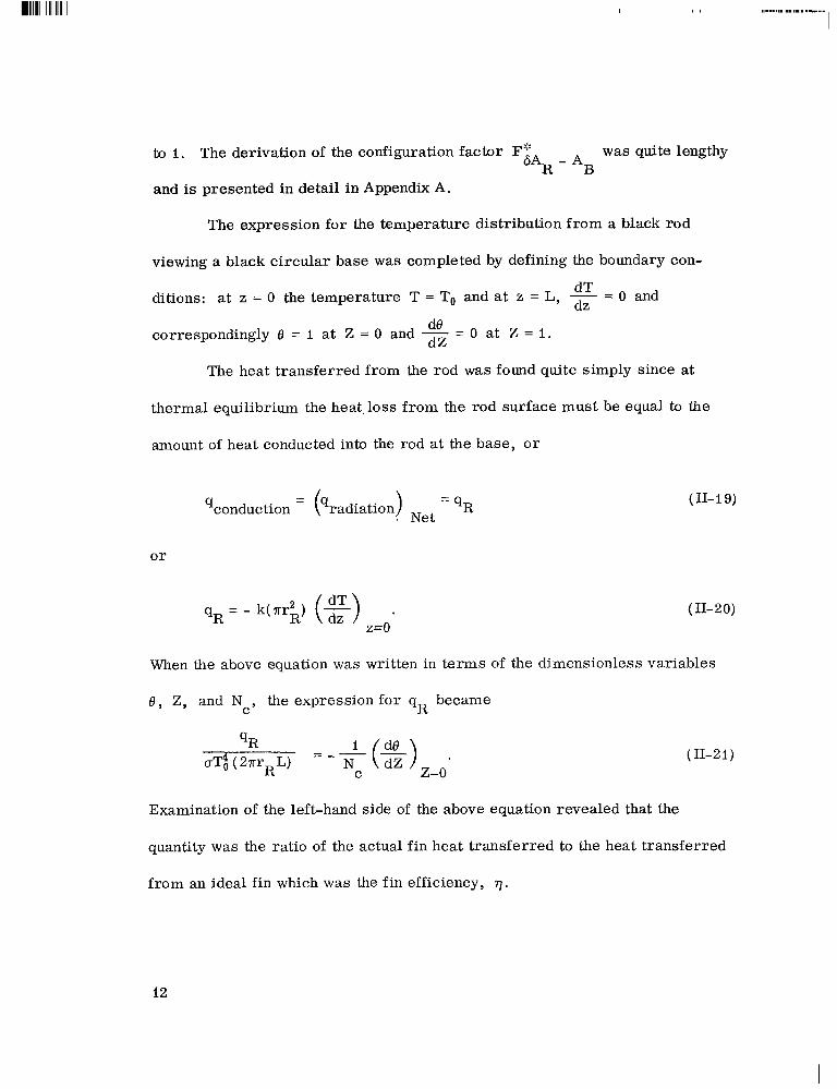
to I.The derivation of the configuration factor F"'6AR - AB w a s quite lengthy

and is presented in detail in Appendix A.

The expression for the temperature distribution from a black rod

viewing a black circular base was completed by defining the boundary con-

-ditions: at z = 0 the temperature T = To and at z = L, dT = O anddz de - 0 at Z = 1 .correspondingly 6 = 1 at Z = 0 and -dZ -

The heat transferred from the rod was found quite simply since at

thermal equilibrium the heat.loss from the rod surface must be equal to the

amount of heat conducted into the rod a t the base, o r

'conduction -- @radiation) Net -- 'R (11-1 9)

or

qR = - k ( m 2 ) (11-20)R z=o

When the above equation w a s written in terms of the dimensionless variables

0 , Z, and Nc, the expression for qR became

UT! ( qR27rrR~) - +(&) . (11-21) C z=o

Examination of the left-hand side of the above equation revealed that the

quantity was the ratio of the actual fin heat transferred to the heat transferred

from an ideal fin which was the fin efficiency, q.

12

Numerical Solution for Black Surfaces

The equation (11-18) for the temperature distribution w a s solved

nlimerically using the Runge-Kutta method. It w a s solved by determining

which of a succession of guessed values of - at Z = 0 led to a solutiondZ dBthat satisfied the boundary condition -dZ = 0, a t Z = 1. A AZ step size

of 0.01 was used for all solutions; however, A Z step sizes of 0.001 and

0.0001 w e r e tried and i t was determined that h e accuracy was not improved.

Solutions were determined for each of the test cases and also for a wide selec­

governed the configuration factor, F 6AR - AB . These data a r e presented in

the curves in Appendix C and typical values of .9 ( Z ) a r e presented in Table

C-1 of Appendix C.

Since the Runge-Kutta integration of equation (11-18) yielded (-)dB ,dZ z=0 the fin efficiency ( q ) o r the fin heat transfer ( qR) w a s easily obtained from

equation (11-21) . The fin efficiency w a s plotted versus the conduction param­

eter for the limiting cases of R2 = R, (no base) , R2 = 03 (infinite base,

F6AR - AB = 0. 5) and two intermediate values of R2 for each of five values

of R,. The results are plotted in Appendix C .

Formulation of Equations for Nonblack Surface

In this section the analysis is extended from the black case to the case

of gray, diffuse emitters and absorbers. When a surface element on the rod

a distance z from the base is considered, the energy that leaves this location

13

This isincludes both the direct emission and the reflected incident energy.

called the radiosity B (energy/unit area-time)

B = + p'H (11-22)

where H is the incident energy per unit time, and E and p' are the

emissivity and reflectivity respectively .

The net heat loss from a surface location w a s B - H and the fin energy

balance was,

(11-23)

where the conduction w a s evaluated the same as in the black analysis. T and

Z were normalized as before

T Z e = - and Z = - L TO

which yielded

d20 2 L2==- ( B R - H R ) .kr ToR (11-24)

When equation (11-24) was multiplied and divided by UT$,and B'k and H"

B H were defined a s B" = 7 and H* = 7, then

ci TO 0-TO

( 11-2 5 )

the base surface radiosity and of theThe irradiation H'* w a s a function ofR

radiation from the surroundings; thus

14

(11-26)

When selective surfaces were not considered, then

(11-27)

where E and p were gray body properties, that is,

The radiosity distribution B"' in equation (11-26) was related to the otherB

energy transfers of the system by the following radiant flux balance

(11-29)

The four equations (11-25) (11-26) (11-27) , and (11-29) in four unknowns

described the temperature distribution of the rod. However, H'"R was

eliminated by use of equation (II-27).

(11-30)

Substitution into equation ( 11-25) yielded

(11-31)

and similarly equation (11-26) yielded

(11-32)

15

-

J-

This yielded three equations in three unknowns, BG, B i , and e ( Z) , the

temperature distribution, which were to be determined.

The problem w a s completed by defining the boundary conditions. A t

dTz = 0 the temperature T = To, and at z = L, -- 0. Correspondingly,dz

e = i at Z = O , and--de - 0 at Z = 1. This nonlinear system of differentialdZ

and integral equations required a simultaneous solution.

Since the case being considered had negligible incident radiant energy,

g( Z) M 0, the system of equations was reduced to

(11-33)

B:: = E e4 + p, J B::: B B B B R 6AB - 6AR (11-34)

AR

B::: = E e4 + p, J B:k p:: R R R B 6AR- 6AB ( 11-3 5)

AB

There were no known exact analytical solutions and therefore a numerical

solution w a s sought.

Numerical Solution for Nonblack Surfaces

The above system of equations could have been solved numerically in

this form by assuming distributions for B"R and B'"B and iterating until the

boundary conditions were satisfied. This would have been quite tedious,

however, since equations (II-34) and (11-35) must first be satisfied. Then,

B"R must be substituted into equation (11-33) to find 6 ( Z ) which must be used

as an input into equations (11-34) and (11-35) until agreement is reached. 16

This process must be repeated until the boundary conditions are satisfied.

Because of the lengthy iteration involved in solving the system in this form,

i t was more expeditious to convert equation (11-33) into an integral form

which included the boundary conditions.

When N was defined as

N E N =- c R

P k

equation (11-33) became

The above equation was integrated from 1 to Z

(s)z=1 = 0 applied to yield

(11-36)

(11-37)

and the boundary condition

(11-38)

where T was a dummy integration variable. Equation (11-38) w a s integrated

from 0 to Z and the boundary condition 0 = 1 a t Z = 0 w a s applied to yield

z 7'

e ( Z ) = I+ N F 4 ( T ) - B ~ ( T ) ]dT d7'. (11-39) 0 1

The above double integral was transformed into two first order integrals using

integration by parts as outlined by Hering [ 191 to yield

(11-40)

17

The above equation could be readily solved by numerical techniques if B’k( T )R

were known.

The procedure outlined by Sparrow and Cess [26] w a s used to

determine B“R ( T ) . The rod and base were considered to be M isothermal

elements. When the-ith element w a s considered, the integral equation (II-35)

for B‘k( T ) w a s expressed as a summationR

(11-41)

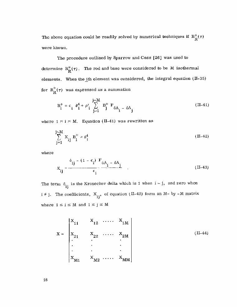
where 1 5 i 5 M. Equation (11-41) w a s rewritten as

(11-42)

where

(11-43)

The term 6.. is the Kronecker delta which is 1 when i = j , and zero when 1J

i # j . The coefficients, X. ., of equation (11-42) form an M- by -M matrix 1J

where 1 i: i 5 M and 1 5 j 5 M

x= x2 1 x22 ..... X2M (11-44)

xMi XM2 ..... xm

18

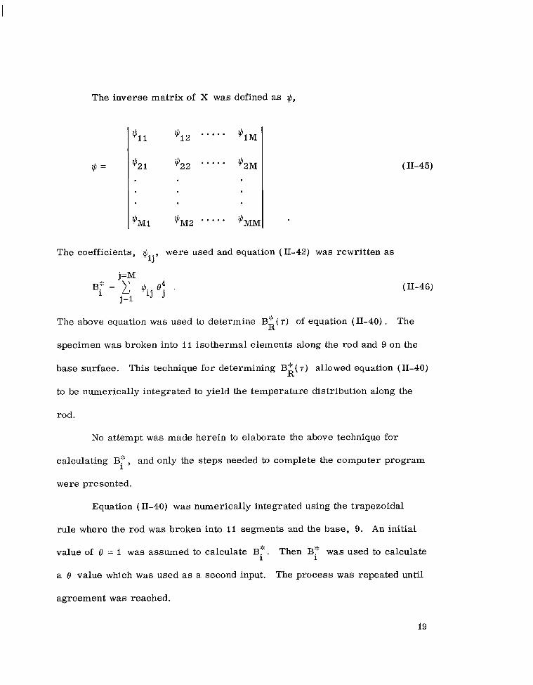
The inverse matrix of X was defined as +,

'II qJi2 ..... 'IM

* = ' 2 I ' 2 2 ..... '2M (11-45)

'MI $hM2 ..... 'Mh 4

The coefficients, iij,w e r e used and equation (11-42) w a s rewritten as

j=MBI:' = Q.. e4 . (11-46)

1 j=1 1~ j

The above equation w a s used to determine B"R ( T ) of equation (11-40) . The

specimen w a s broken into I 1 isothermal elements along the rod and 9 on the

base surface. This technique for determining B"'R( T ) allowed equation (11-40)

to be numerically integrated to yield the temperature distribution along the

rod.

No attempt was made herein to elaborate the above technique for

calculating BF , and only the steps needed to complete the computer program

were presented.

Equation ( 11-40) w a s numerically integrated using the trapezoidal

rule where the rod was broken into 11 segments and the base, 9. An initial

value of 8 = Iwas assumed to calculate B". Then BI:' was used to calculatei 1

a e value which w a s used as a second input. The process was repeated until

agreement was reached.

19

Since this solution did not directly yield the value for (g) as did~

z=I the Runge-Kutta solution for the black case, the heat transfer was calculated

by determining the slope at Z=O using the following numerical differentiation

formula [ 271:

(11-47)

The subscripts refer to the beginning points of the first five isothermal

elements of the rod. By using this value for (s) the rod heat Z=O

transfer was determined as before, using equation (11-21) .

EXPERIMENTAL INVESTIGATION

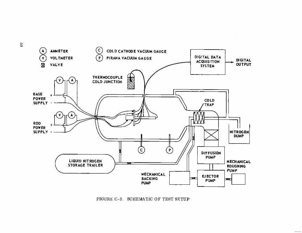
The experimental setup consisted of the test specimen, the high

altitude simulation system, and the data acquisition system as illustrated in

Figure C - 3 of Appendix C . A detailed description of the high altitude simula­

tion system and the data acquisition system is presented in Appendix B.

The test specimen consisted of two prime parts - the 2 . 54-cm (I-inch)

diameter aluminum rod and the flat circular 20.32-cm (8-inch) diameter

aluminum base. Both the base and the rod had individual heating elements.

The base was designed in two halves so that it could be mounted on the rod

without disturbing the heater and the thermocouples previously used to

determine the temperature distribution of the rod alone.

20

Base

The base surface consisted of two halves of a circular plate (mounting

attachments so that the base could be fixed to the rod) , a heater element on

each half, and 12 thermocouples spot-welded to the base surface viewing the

fin as shown in Figure C-2. Three different heater arrangements w e r e

bench tested before a satisfactory temperature distribution w a s obtained. The

configuration selected w a s one with heater wires closely spaced in a c i rcu lar

pattern.

The base heater w a s constructed in the following manner. Two heater

w i r e terminal posts were affixed to each half of the base and the surface was

then covered with a layer of f iberglass tape to electrically insulate the heater

w i r e and base surface. Then 16-gauge Chromel-A resis tance w i r e with a

resistance of 0.830 ohms per meter (0.253 ohms per foot) w a s wound

circumferentially on each half of the base. The heater wire w a s covered by

a layer of asbestos (0.318 cm thick) ; this w a s held in place by a piece of

aluminum sheet stock (0.079 c m thick) attached to the base by screws. The

resis tances of the base surface hea ters were measured and foundto b e 5 ohms

each.

For bench testing the base specimen hea ters were connected to a

30-volt, 10-amp, DC power supply. The current to the heater wi re was

controlled by a variable resistance. The thermocouple cold junction reference

w a s an ice bath and the thermocouple millivolt output w a s recorded on a s t r ip

21

l1l11l11l1l1111111111llI I I ..... .

chart by a Brown-Marco recording system. Several tests w e r e conducted at

different power levels and the base temperature spread w a s determined after

steady state w a s reached. Steady state w a s normally achieved in about three-

fourths of an hour. The tests were conducted at room temperature of

approximately 297. 6°K (76O F) .

The base heater configuration selected produced a maximum tempera­

ture differential of 8" F a t an average surface temperature of 388.7O K (240" F) . This was considered acceptable since the temperature distribution w a s expected

to be much more uniform in vacuum.

Fin

The rod o r fin portion of the test specimen consi:ted of an aluminum

alloy rod, a heater element, and 48 thermocouples as shown in Figure (3-1.

The rod specimen was a 2.54-cm (I-inch) diameter 6061 T6 aluminum alloy rod

approximately 60.96 c m (24 inches) long. One end of the rod was circum­

ferentially wound for approximately 10.16 c m (4inches) with a heater wire; the

remainder of the rod contained 48 thermocouples evenly spaced at 12 stations;

the end of the rod opposite the heater had 4 thermocouples spot-welded to the

end which was covered with one-fourth inch of insulation. The 48 thermocouples

3 were located at intervals of 4.45 c m ( 1 7 inches) with 4 couples at each station.

The 4 thermocouples at each station were evenly spaced around the circumference

of the rod.

The fin heater was constructed in the following manner. First, the rod

22

was wrapped with a layer of f iberglass tape to electrically insulate the heater

w i r e f rom the rod. The heater wire w a s then attached to one terminal post

and wound around the rod and attached to the second terminal post. It w a s then

coated with a layer of Ceramacoat 512 (AREMCO Products, Inc. , Briarcliff

Manor, New York) and wrapped with a I.27-cm (1/2-inch) layer of asbestos

cloth. The heater resistance w a s measured and found to be I.16 ohms.

The power input to the rod and a l so to the base w a s a closely regulated

DC power supply, Variable res is tances w e r e placed in both base and rod

power leads s o that the desired power supply could be accurately achieved.

The power input w a s determined by two Hewlett-Packard model 3430A digital

voltmeters. One measured the system voltage drop and the other measured the

voltage across a known resistance placed in one leg of the circuit.

Test Setup

The test specimen w a s suspended in the vacuum chamber by a cord at

either end of the specimen which attached to a horizontal c r o s s member as

shown in Figure C-I. The test specimen thermocouple leads w e r e taped to the

supporting c ros s member and then fed through the chamber w a l l with a standard

vacuum feedthrough connector. A thermocouple cold junction, ice bath, w a s

located adjacent to the chamber and then the thermocouples w e r e connected with

the data acquisition system. The test specimen power leads were similarly fed

through the vacuum chamber wall and connected to the regulated DC power

source. Separate vacuum feedthrough connectors w e r e used for the power

leads and thermocouples to avoid any interference.

23

The vacuum chamber wal ls were painted black to minimize the reflected

energy. To prevent the complications of having to account for an incident

energy distribution on the specimen, the vacuum chamber wall w a s maintained

at 78.7OK (-318OF) by circulating liquid nitrogen through the vacuum chamber

wall. The temperature distribution of the rod without the base was solved

numerically, including the sink temperature of 78.7"K to verify that the

incident energy w a s negligible. The inclusion of the incident energy w a s

calculated to produce less than 0.1% change in the temperature at the end of

the rod.

Experimental Procedure

The test was designed to explore the temperature range f rom ambient

to approximately 533"K (500" F) . Based on the ea r i l e r rod tests by Shouman,

approximate values of the rod temperature were known for various power inputs

to the rod heater. Also, it was known that approximately 8 hours were

required to achieve steady state heat transfer. Seven of the 20 test runs were

conducted on a single 8-hour shift. For these runs the rod and base power

supplies were left on overnight to permit fas te r achievement of steady state

conditions. Steady state w a s considered achieved when all temperatures on

the rod varied less than I degree per hour. This assumption was wel l borne

out by longer runs that permitted a steady state condition where essentially

no temperature variations were noticeable.

24

The test runs are summarized in Tables C-2 and C-3 of Appendix C.

Test runs I through 7 were conducted with the base installed. Test runs 8, 9,

and 10 w e r e conducted with the rod only, and runs 11, 12, and 13 w e r e con­

ducted with the rod only and a smoke black carbon coating. Test runs 14

through 17 were conducted with the base installed and both the base and the

rod carbon coated. Test runs 18, 19, and 20 w e r e a repeat of run 12 to study

the effect of removing the thermocouples. All test runs, except the first one,

were made with liquid nitrogen cooling the chamber wal l s .

The initial test w a s conducted without liquid nitrogen and without

power to the base to observe the effect of the presence of the base. This w a s

an abbreviated test run and the thermal equilibrium was questionable. Test 2

w a s a repeat of test I but with liquid nitrogen in the cooling jacket.

Since the test specimen had individual heaters on the rod and base, it

was highly impractical f rom a time standpoint to achieve equal temperatures

on the base and the fin at the base fin intersection. Because of this problem

the tests with the base were planned to achieve a somewhat higher and a some­

what lower temperature than the fin temperature a t the base. Tes t 3 and test 4

satisfied this requirement f o r the initial power setting to the rod. For tests 5,

6 , and 7 the procedure for tes ts 2 , 3 , and 4 w a s repeated with a different power

supply to the rod heater as shown in Table C-2 of Appendix C.

The base w a s removed and tests 8, 9, and 10 were conducted with

three different power inputs to the rod heater. These data were desired so

25

that the case of base surface interaction could be compared to the rod only,

without interactions.

A carbon black coating was applied to the rod and base to obtain data

that would satisfy a black surface analysis. The coating w a s applied by holding

an acetylene torch burning an acetylene r ich mixture near the specimen and

rotating it until a velvety black coating was obtained over the entire surface of

the rod and base. Tes ts 11, 12, and 13 were then made using the rod only.

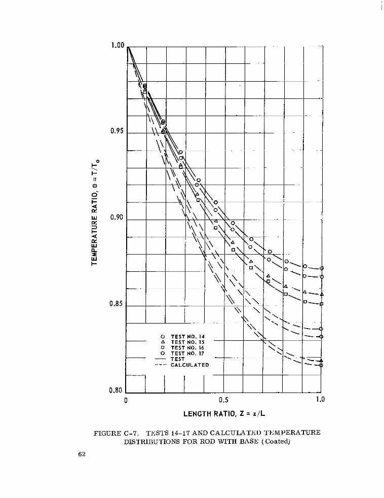
These tests w e r e s imi la r to tes ts 8, 9, and 10. Tests 14, 15, 16, and 17 were

then conducted with the base installed. The procedure w a s again to obtain data

with the base temperature somewhat above and below the rod temperature.

Test runs 18, 19, and 20 were then conducted with the rod only to

ascertain the effect of the thermocouples mounted on the rod. The power

input fo r these tests w a s maintained the same as for test 12. F o r test 18,

one-half of the thermocouples were removed leaving 2 thermocouples at each

of 12 stations. For test 19 , one-half of the remaining thermocouples were

removed leaving I thermocouple a t each station except the fifth station which

had none. Test 20 w a s conducted with 1 thermocouple at the heater end and

1 at the insulated end of the rod.

The test procedure w a s essentially the same for all test runs once the

specimen w a s prepared for that particular test. The test runs were begun by

simultaneously turning on the data acquisition system, the power 'supply to the

specimen heaters, the backing pump, the heaters to the ejector pump and

diffusion pump, the cooling water to the pump condensers, and then pressurizing

26

.\ the liquid nitrogen storage trailer (for test runs I through 7 the specimen

heater power supply w a s turned on the previous day and left on all night).

When the diffusion and ejector pump oil reached approximately 545°K (520" F) ,

the roughing pump was turned on and the liquid nitrogen flow to the pumping

system cold trap and to the vacuum chamber cooling jacket was begun. The

vacuum was then read on the P i ran i gauge and the system w a s switched to

"hi-vacuum, If or onto the diffusion and ejector pumps when the vacuum reached

150 microns.

A f t e r hi-vacuum operation w a s achieved, the procedure consisted of

checking the vacuum, thermocouple ice bath, heater power supply readings,

and the specimen temperature distribution periodically. The specimen

temperature w a s observed until steady state w a s achieved and then a new test

run was begun by changing the power inputs to the specimen. Once a test run

o r series of runs w a s completed all of the test equipment w a s turned off and

the nitrogen storage trailer vented. The cooling water t o the ejector and

diffusion pump oil condenser w a s left on fo r approximately 2 hours to protect

solder joints .

27

RESULTS

Test Cases

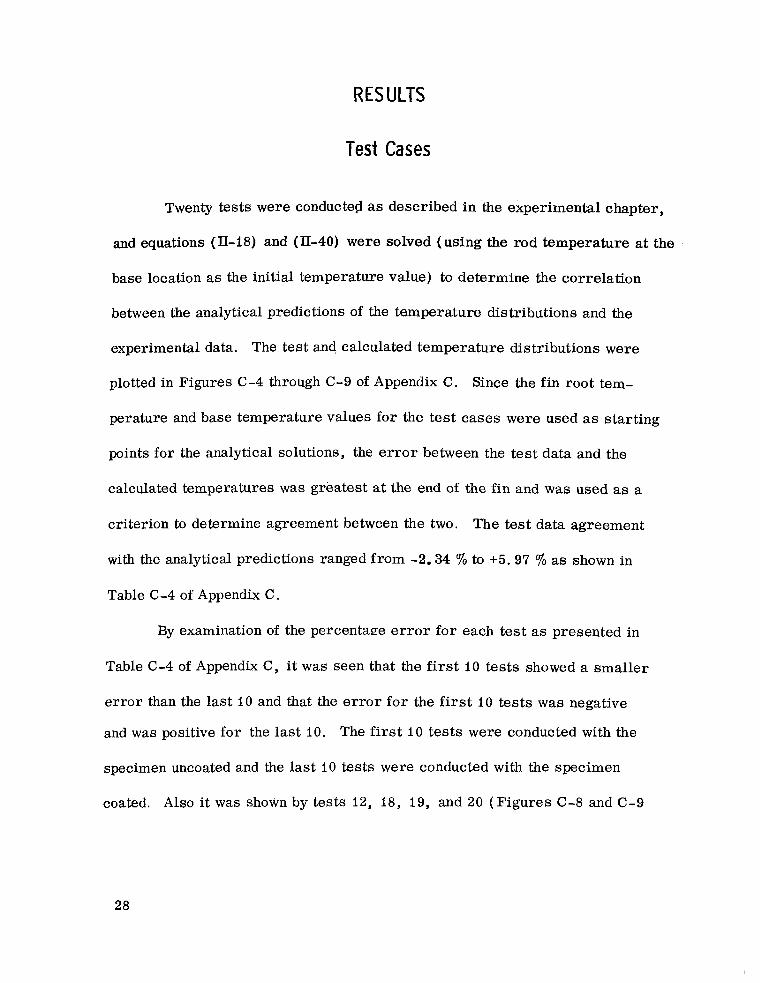
Twenty tests were conducted as described in 'the experimental chapter,

and equations (II-18) and (II-40) were solved (using the rod temperature at the

base location as the initial temperature value) to determine the correlation

between the analytical predictions of the temperature distributions and the

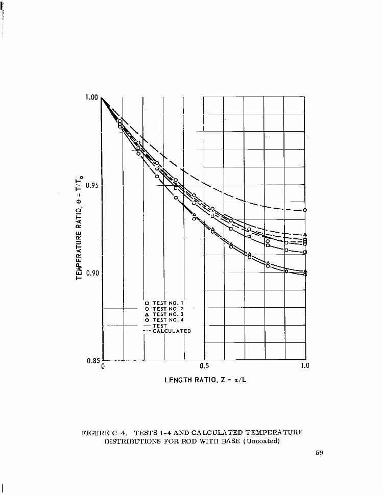
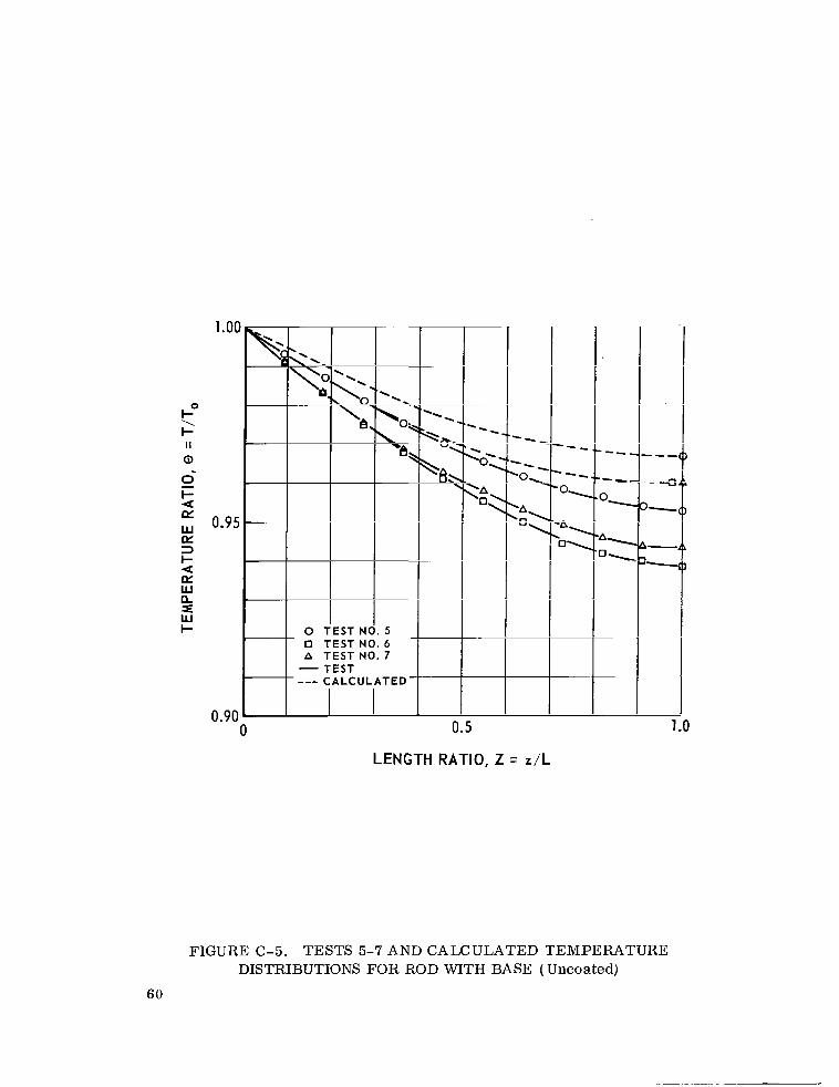
experimental data. The test and calculated temperature distributions were

plotted in Figures C-4 through C-9 of Appendix C. Since the fin root tem­

perature and base temperature values fo r the test cases were used as start ing

points for the analytical solutions, the e r r o r between the test data and the

calculated temperatures was greatest at the end of the fin and w a s used as a

criterion to determine agreement between the two. The test data agreement

with the analytical predictions ranged f rom -2.34 % to +5.97 % as shown in

Table C-4 of Appendix C.

By examination of the percentage e r r o r fo r each test as presented in

Table C-4 of Appendix C y it w a s seen that the first 10 tests showed a smal le r

e r r o r than the last 10 and that the e r r o r f o r the f i r s t 10 tests w a s negative

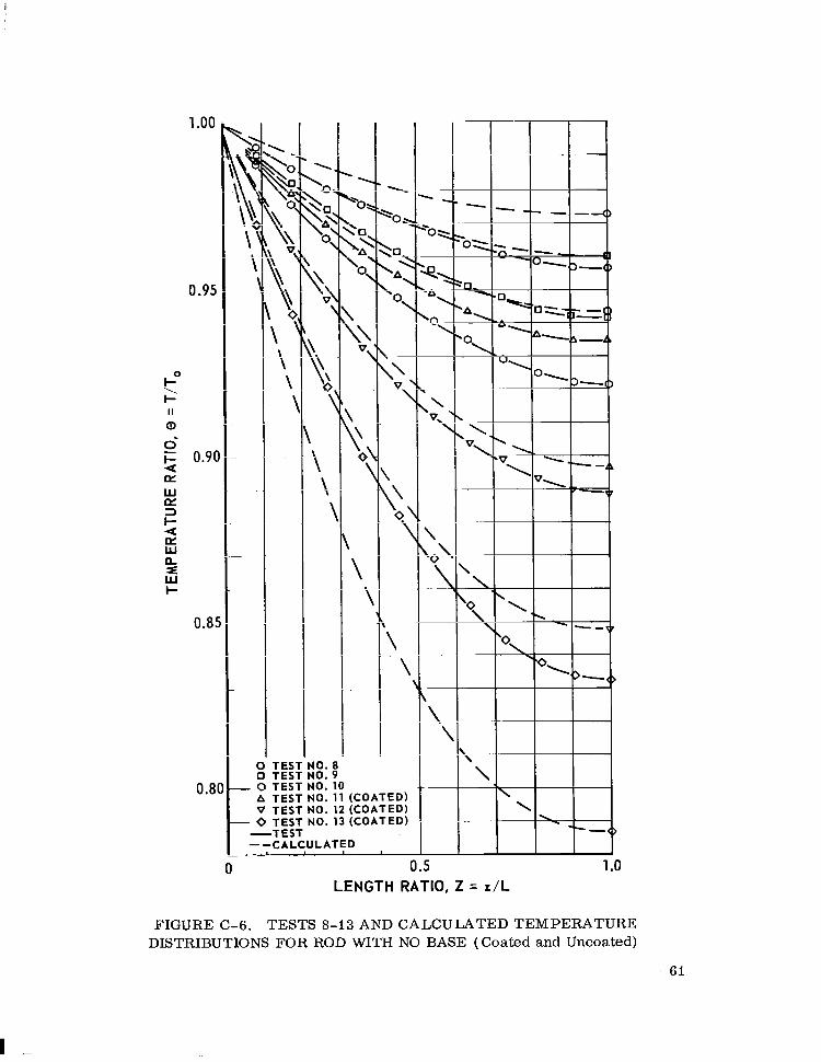
and was positive for the last I O . The first 10 tests were conducted with the

specimen uncoated and the las t 10 tests were conducted with the specimen

coated. Also it was shown by tests 12, 18, 19, and 20 (Figures C-8 and C-9

28

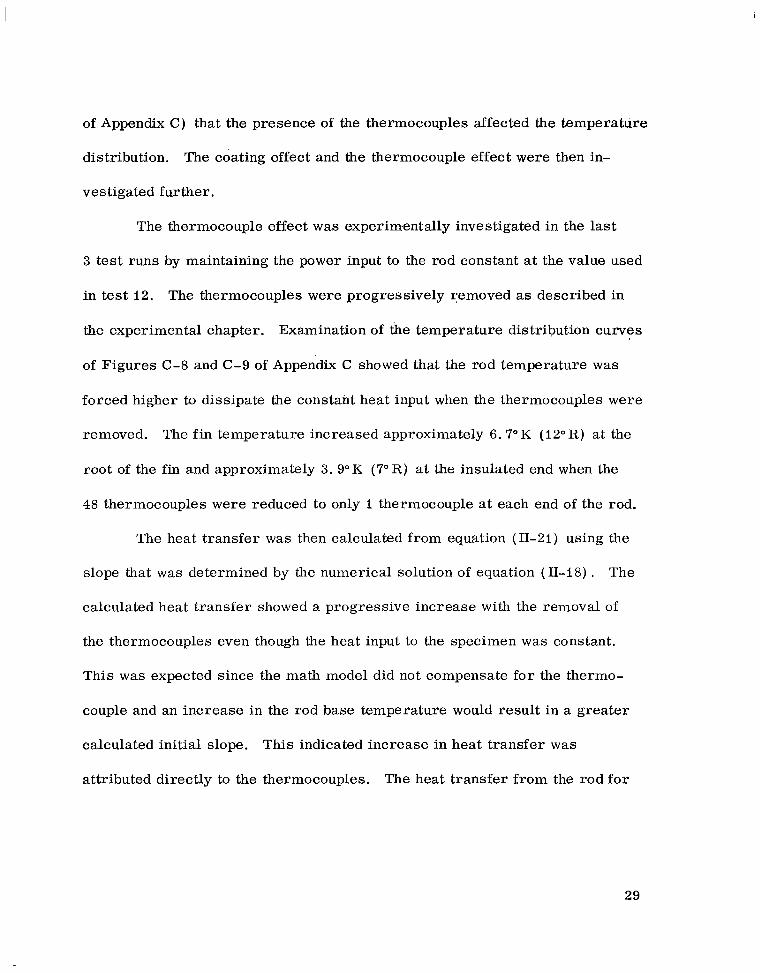
of Appendix C ) that the presence of the thermocouples affected the temperature

distribution. The coating effect and the thermocouple effect w e r e then in­

vestigated further.

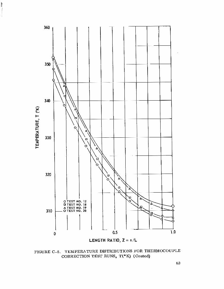
The thermocouple effect w a s experimentally investigated in the last

3 test runs by maintaining the power input to the rod constant at the value used

in test 12. The thermocouples w e r e progressively removed as described in

the experimental chapter. Examination of the temperature distribution curves

of Figures C-8 and C-9 of Appendix C showed that the rod temperature w a s

forced higher to dissipate the constant heat input when the thermocouples were

removed. The fin temperature increased approximately 6.7" K (12" R) at the

root of the fin and approximately 3.9"K (7"R) at the insulated end when the

48 thermocouples were reduced to only I thermocouple at each end of the rod.

The heat t ransfer was then calculated from equation (11-21) using the

slope that w a s determined by the numerical solution of equation ( I I - I 8 ) . The

calculated heat transfer showed a progressive increase with the removal of

the thermocouples even though the heat input to the specimen w a s constant.

This w a s expected since the math model did not compensate for the thermo­

couple and an increase in the rod base temperature would result in a greater

calculated initial slope. This indicated increase in heat transfer w a s

attributed directly to the thermocouples. The heat transfer f rom the rod fo r

29

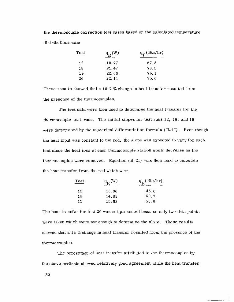
the thermocouple correction test cases based on the calculated temperature

distributions was:

Test qE (W ‘IR‘Btu/hr) -~

12 19.77 67. 5 18 21.47 73.3 19 22.00 75.1 20 22.14 75. 6

These results showed that a 10.7 7’0 change in heat transfer resulted from

the presence of the thermocouples.

The test data were then used to determine the heat transfer for the

thermocouple test runs. The initial slopes for test runs 12, 18, and 19

were determined by the numerical differentiation formula (II-47) . Even though

the heat input w a s constant to the rod, the slope was expected to vary for each

test since the heat loss at each thermocouple station would decrease as the

thermocouples were removed. Equation (II-21) w a s then used to calculate

the heat transfer from the rod which was:

Test-

12 13.36 18 14.85 19 15.52

45. 6 50. 7 53.0

The heat transfer for test 20 was not presented because only two data points

were taken which were not enough to determine the slope. These results

showed that a 14 % change in heat transfer resulted from the presence of the

thermocouples.

The percentage of heat transfer attributed to Lhe thermocouples by

the above methods showed relatively good agreement while the heat transfer

30

showed a wide disparity. The heat transfer based on he test data was con­

siderably lower than that based on the analytical solution, and as noted before

the temperature e r r o r went from negative to positive and increased in

magnitude when the surface coating was added. Based on these results, the

coating used on the last 10 test runs apparently induced more e r r o r (and in

the opposite direction) than the thermocouples. Further quantitative analysis

of the thermocouple effect did not appear meaningful because of the coating

effect and because the heat transfer from the rod cannot be precisely deter­

mined. The heat input to the specimen w a s precisely measured but it could

not be accurately determined what amount of heat w a s lost from the rod and

what amount w a s lost from the heater portion of the test specimen.

The specimen w a s coated after the thermocouples were installed and

therefore the layer of coating actually insulated the surface of the rod and the

thermocouples. Consequently, the thermocouples were reading the rod

surface temperature and therefore indicated a temperature higher than the

surface temperature of the coating. To study this effect, test 19 was used

because i t had the fewest number of thermocouples and yet provided a data

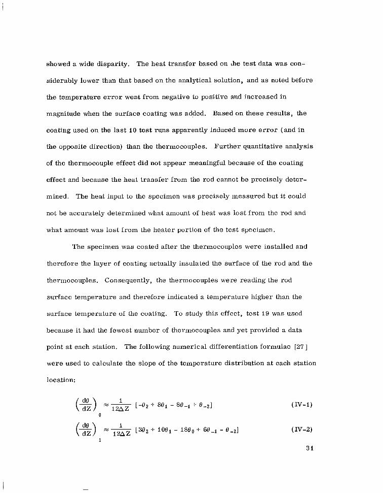
point at each station. The following numerical differentiation formulae [27 ]

were used to calculate the slope of the temperature distribution a t each station

location:

(IV-2)

31

-2

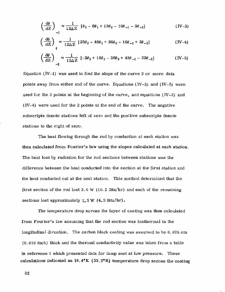
Equation (IV-I) w a s used to find the slope of the curve 3 or more data

points away from either end of the curve. Equations ( N - 3 ) and (IV-5) were

used for the 2 points at the beginning of the curve, and equations ( N - 2 ) and

(IV-4) were used for the 2 points at the end of the curve. The negative

subscripts denote stations left of zero and the positive subscr ipts denote

stations to the right of zero.

The heat flowing through the rod by conduction a t each station was

then calculated f r o m Fourier ' s law using the slopes calculated at each station.

The heat lost by radiation fo r the rod sections between stations was the

difference between the heat conducted into the section at the first station and

the heat conducted out a t the next station. This method determined that the

first section of the rod lost 3 . 0 W (IO.2 Btu/hr) and each of the remaining

sections lost approximately i. 3 W (4.3 Btu/hr) . The temperature drop across the layer of coating was then calculated

f rom Fourier ' s law assuming that the rod section was iosthermal in the

longitudinal direction. The carbon black coating w a s assumed to be 0.025 c m

(0.010 inch) thick and the thermal conductivity value w a s taken f rom a table

in reference I which presented data for lamp soot at low pressure. These

calculations indicated an 18.4.K (33.2.R) temperature drop ac ross the coating

32

on the first section and approximately 7.8" K (14"R) ac ross the coating on the

remaining sections.

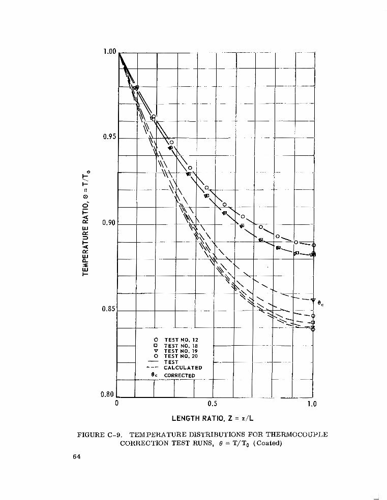
A corrected temperature distribution w a s then computed f rom equation

(II-18) using an initial temperature equal to the indicated test temperature \

minus 18.4"q 3 . 2 . R) o r 333. OoK (599.37.R) . This curve was plotted in

Figure C-9 of Appendix C and designated 0 . The test data disagreement w a s C

reduced f rom 4.9 % to 3.2 % based on the end point temperature. Although

this did not explain the e r r o r in the data, it did indicate a trend in the proper

direction to explain the positive e r r o r fo r each case where the coating w a s

applied. Other variables which could not be accurately determined were the

actual thickness and the thermal conductivity of the coating. Also, the coating

w a s of a porous nature with a velvety surface composed of many small peaks

and valleys which would radiate f rom some point beneath the actual surface.

This compounded the problem of determining the coating thickness.

Parameter Study

In addition to the analytical predictions of the test cases , several

temperature distributions w e r e calculated using equation ( 11-18) by varying

the governing dimensionless parameters . The black case w a s the only one

considered since f o r efficient heat t ransfer the surface would be made as

black as possible. The configuration factor FdAR - AB w a s plotted versus

the length of the rod, in 'Figure C-IO of Appendix C, for the test specimen

case to visualize how it affected the temperature distribution equation (II-18)

33

where 8 = 1.B

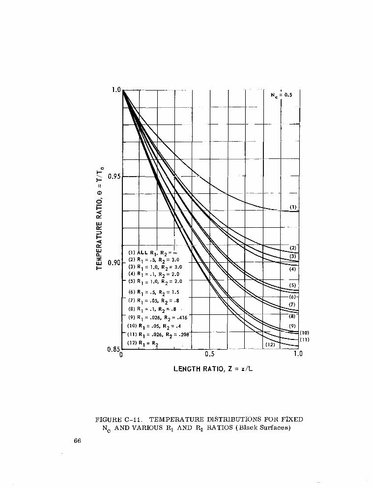
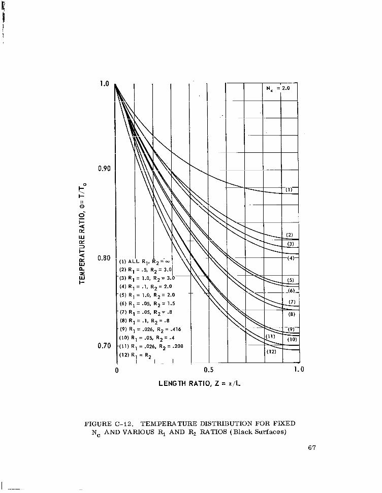
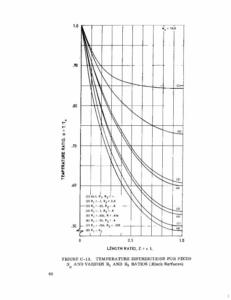
The above equation was then solved for values of N C

of 0.5, 2, and

10. The dimensionless ratios, R, and R2, which appeared in the term

- AB w e r e varied over a wide range. The limiting cases of no base

and an infinite base were also solved for each value of N . The resulting c .

temperature distributions were plotted in Figures C-11, C-12, and C-13

of Appendix C

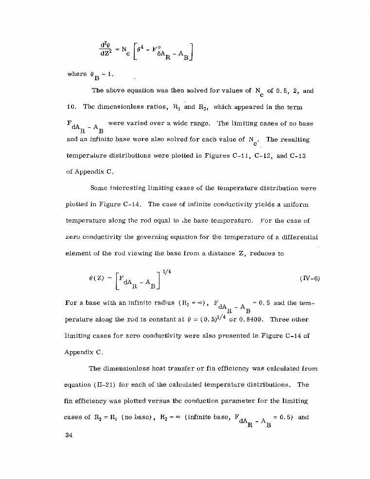
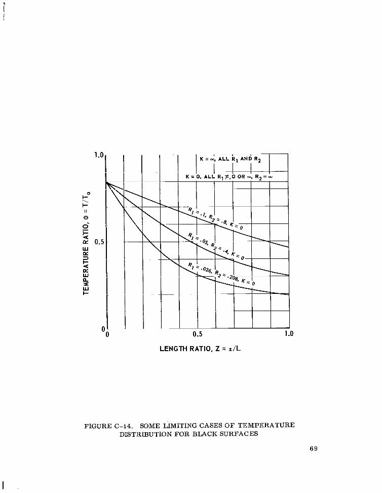
Some interesting limiting cases of the temperature distribution w e r e

plotted in Figure C-14. The case of infinite conductivity yields a uniform

temperature along the rod equal to h e base temperature. For the case of

zero conductivity the governing equation for the temperature of a differential

element of the rod viewing the base from a distance Z , reduces to

For a base with an infinite radius (R2= w ) , FdAR - AB = 0 . 5 and the tem-

Three otherperature along the rod is constant a t 0 = (0 . 5)'14 o r 0.8409.

limiting cases for zero conductivity were also presented in Figure C-14 of

Appendix C .

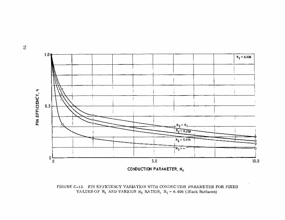
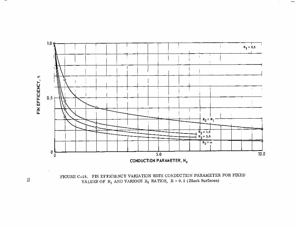
The dimensionless heat transfer o r fin efficiency was calculated from

equation (11-21) for each of the calculated temperature distributions. The

fin efficiency w a s plotted versus the conduction parameter for the limiting

cases of R, = R, (no base), R2 = (infinite base, - AB = 0.5) and

34

two intermediate values of R2 for each value of q. The results are presented

in Appendix C in Figures C-15, C-16, C-17, C-18, and C-19. From these

curves it is seen that a low value of N is required to maintain a highC

efficiency, Also it was observed that the fin efficiency for values of N > 0.05 C

was decreased by approximately 50 % from the no base condition to an infinite

base for all values of Ri considered.

The temperature distribution curves and efficiency curves are

applicable to gray surfaces if only singly reflected radiation rays are con­

sidered. It is only necessary to change the N to N' where N' = E N . C C C C

CONCLUSIONS

The experimental data and the numerical solutions showed reasonable

trend agreement. The experimental data, however, were substantially

affected by two identified sources of error :

1. the heat conducted from the rod by the thermocouples

2. the insulation effect of the carbon coating covering the rod surface

and the thermocouple junction.

The above mentioned e r ro r s would tend to invalidate the assumption of one-

dimensional heat transfer. Also the fact that the thermal properties of the

specimen material were assumed constant would induce some e r r o r since E

and k would vary somewhat with temperature. The emissivity could vary with

35

I

t ime from test to test since some surface oxidation would occur. As a result

of these e r r o r s the data did not agree with the analytical predictions as closely

as was desirable for use in quantitative predictions. The trends did agree,

however, and the data were within the range of the identified e r r o r s in the

experiment.

The calculated temperature distributions for a given value of the

conduction parameter w e r e bounded by the cases of no base, and an infinite

base; the temperature spread between the two cases increased with increasing

N . The temperature distribution t raversed the range between the limiting

cases as the values of R, and R2were varied such that the configuration factor

between the rod and the base varied from 0 to 0.5.

The heat t ransfer f rom a rod o r the rod efficiency may vary a large

amount with changing base s ize . The variation may be as much as approxi­

mately 50% for values of N 2 0.05. C

George C. Marshall Space Flight Center National Aeronautics and Space Administration

Marshall Space Flight Center, Alabama 35812, July 1968 124-09-05-00-62

36

C

APPENDIX A.

CONFIGURATION FACTOR ANALYSIS

Configuration Factor F& R ' A B

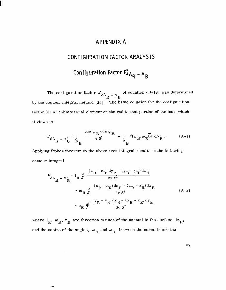
The configuration factor F6AR - AB of equation (11-18) w a s determined

by the contour integral method [ 2 6 ] . The basic equation for the configuration

factor for an infinitesimal element on the rod to that portion of the base which

i t views is

Applying Stokes theorem to the above area integral results in the following

contour integral

where 1R' mR' nR are direction msines of the normal to the surface dAR' and the cosine of the angles, 'pB and 'p R' between the normals and the

37

Y

A vector S, connecting the differential areas has been written as the scalar

A A A products of nR 5R B

and nB SBR. The contour integral equation w a s

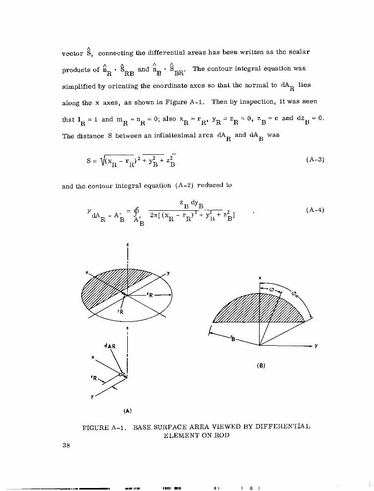
simplified by orienting the coordinate axes so that the normal to dAR lies

along the x axes, as shown in Figure A-1. Then by inspection, i t was seen

-that 1R = 1 and mR = nR = 0; also xR = rR, yR - zR = 0, zB = c and dzB = 0.

The distance S between an infinitesimal area dAR and dAB was

2s = $x R

- rR)2 + yB+ z; (A-3)

and the contour integral equation (A-2) reduced to

'B dYB FdA R - A 'B = PA b ~ + Z B z

2 , 1

(-4-4)

z

z I

'R$ FIGURE A-1. BASE SURFACE AREA VIEWED BY DIFFERENTIAL

ELEMENT ON ROD 38

1.1111 11.1111 II I I II I

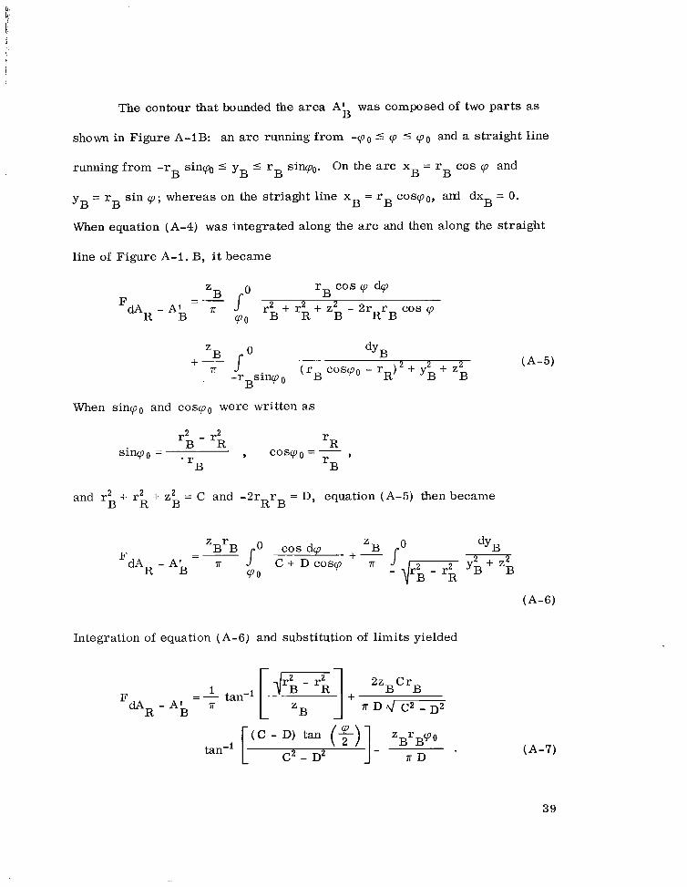
The contour that bounded the area A b was composed of two parts as

shown in F igure A-IB: an arc running f r o m -cpo 5 cp 5 cpo and a s t ra ight l ine

running f r o m -r B sin* 5 y B 5 r B sincpo. On the arc xB = rB c o s cp and

yB = rB s in cp; whereas on the s t r i agh t l ine xB = rBcoscpoy a d dxB = 0.

When equation (A-4) was integrated along the arc and then along the s t ra ight

l ine of F igure A-1. By it became

Z B rB c o s y dcp

r2 + r2 + z2 - 2 r rR - A '

B a

~ p o B R B R B cos cp

When sincpo and coscpo were writ ten as

r2 - r2 rB R Rsincpo = coscpo=- r y- rB B

and r2 + r2 + z2 = C and -2r rB R B R B = D, equation (A-5) then became

Integration of equation (A-6) and substitution of l imi t s yielded

(A-7)

39

+-'tan-'

The term tan (9)was expressed as

and substituted into equation (A-7) . When the appropriate substitutions were

made for C and D and when cpo

configuration factor became

Z B 21rrR

was written as tan-', the expression for the

II."-.' BrR R 1 . (A-9)

When the above equation w a s nondimensionalized with respect to L, and R,,

Rz, and Z were defined as R, = rR/L, R2 = rB/L, and Z = zB/L, the

nondimensional configuration factor became

( A-1 0)

40

I

and from symmetry

(A-1 1)

Configuration Factors FSAR - sAB and 'SA B - 'AR

It w a s readily seen from the cylindrical symmetry of the specimen

that the flux density at any arbitrary radius p on the base was constant for any

arbitrary angle cp. The same w a s true for any cp position on the rod a t a

given z.

Now when a differential slice of the rod and a differential ring on the

base were considered, i t w a s seen that the radiosity distribution w a s uniform

with the coordinate angle cp. However, the radiosity distribution varied along

the length of the rod and also along any radius on the base.

Also from symmetry, the configuration factor from a differential

element on the rod to the portion of a differential ring viewed on the base was

equal to the configuration factor from the total differential ring around the

rod to the total differential ring on the base, o r

(A-I 2)

then

(A-I 3)

41

I

o r

(A-14)

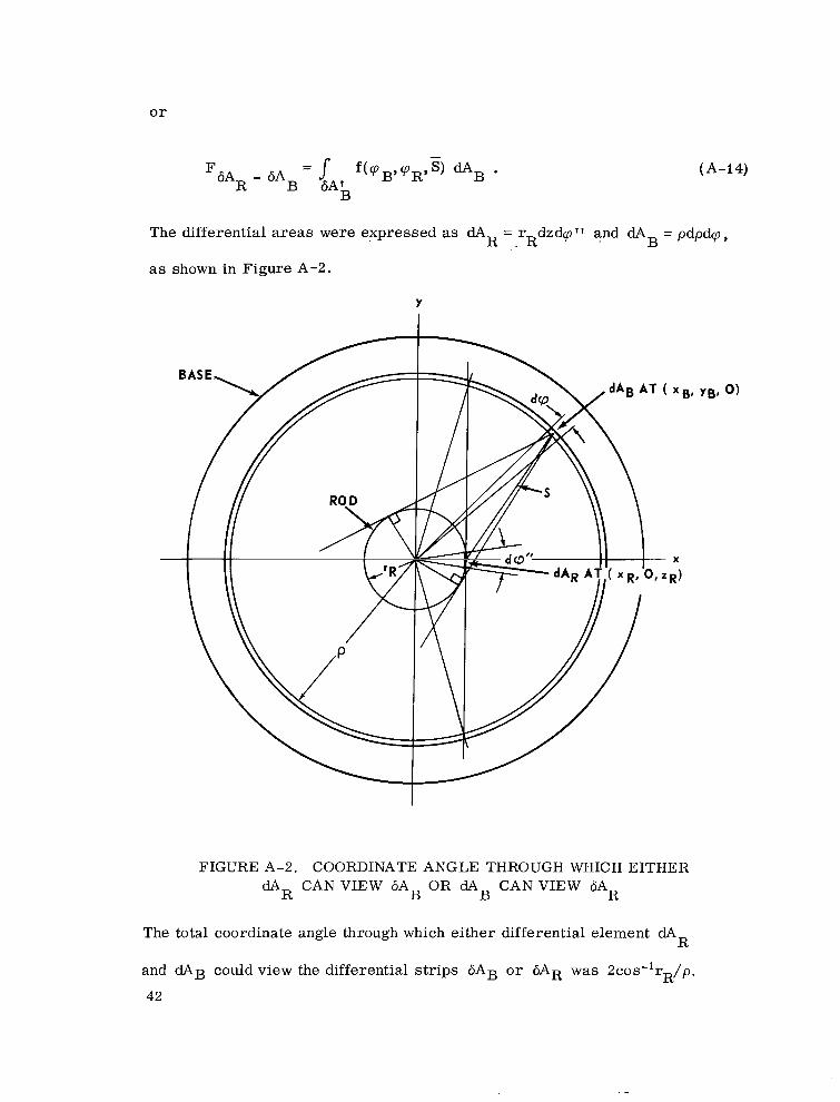
The differential areas were expressed as dAR = r, . Rdzdq" and dAB = pdpdq ,

as shown in Figure A-2.

Y

FIGURE A-2. COORDINATE ANGLE THROUGH WHICH EITHER dAR CANVIEW 6AB OR dA CANVIEW 6AR

B

The total coordinate angle through which either differential element dAR

and dAg could view the differential strips 6AB o r 6AR w a s 2cos-lrR/p.

42

--

-

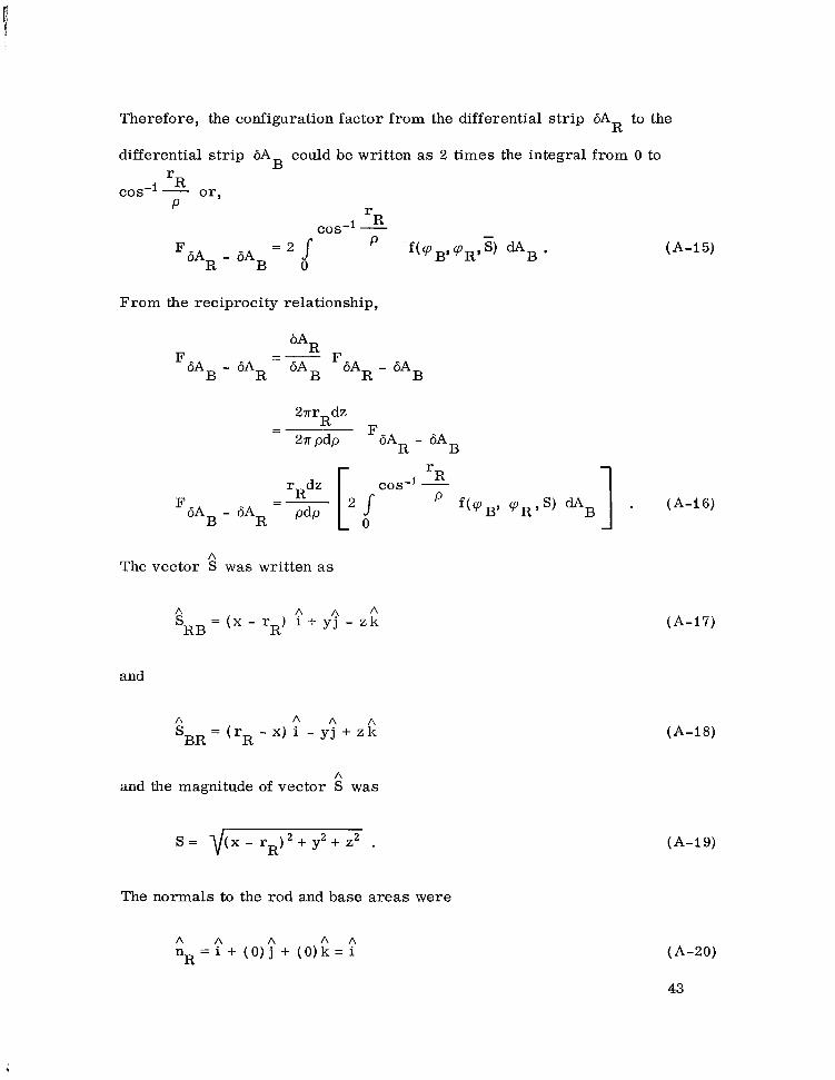
Therefore, the configuration factor from the differential strip 6AR to the

differential strip 6AB could be written as 2 times the integral from 0 to

(A-I 5)

From the reciprocity relationship,

bAR-F 6AB - 6AR 6AB F6AR - 6A B

27rr dzR-

2.rrpdp F6A R - 6A B rR

F6AB - 6AR

f(cpB’ gDR’S) dAB 1 . (A-16)

A The vector S w a s written as

A O O ASRB = ( x - r ) i + y ~ - z kR

and

A A A A- - x) i - y j + z k‘BR - ( r ~

A and the magnitude of vector S was

The normals to the rod and base areas were

A A A A A nR = i + ( 0 ) j + ( O ) k = i

(A-17)

(A-18)

(A-I 9)

(A-20)

43

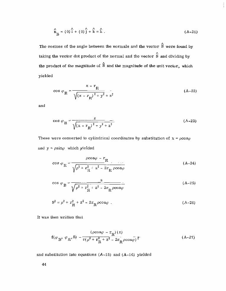
A A A A A n

B = (0 ) i + (0 ) j + k = k . (A-21)

A The cosines of the angle between the normals and the vector S were found by

A taking the vector dot product of the normal and the vector S and dividing by

the product of the magnitude of fi and the magnitude of the unit vector, which

yielded

x - r R 'Os 'R = ~ ( x 2 + y2 + 2 2

(A-22)- r

R

and

c o s q = f ( x - r j 2 + y2 + z2

(A-23)

R

These were converted to cylindrical coordinates by substitution of x = pcoscp

and y = psincp which yielded

pcOscp - rR ~ .~~ (A-24)cos cp R = p2 + r; + z2 - 2 r

R pcosq

Z -cos cp B = - (A-25) p2 + r2 + z2 - 2rR pcoscpR

(A-26)

It was then written that

(A-27)

and substitution into equations (A-15) and (A-16) yielded

44

-

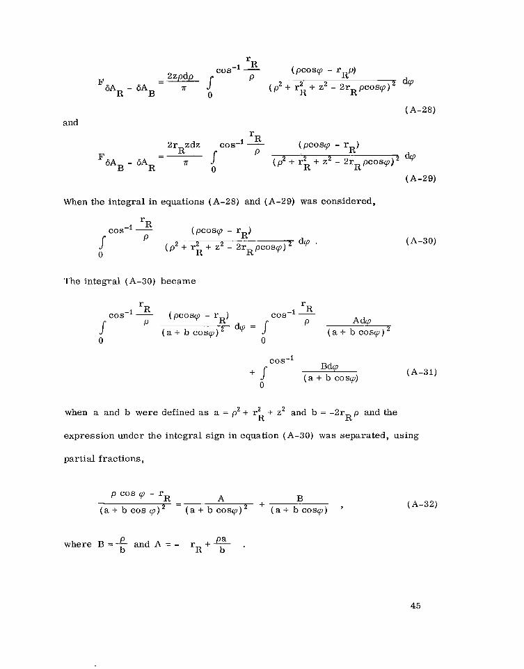
rR (PCOScp - rRP)

-7r

dcpF6AR - 6A -2zpdp scos-i -

P (p2+ r2R + z2 - 2 rR p ~ o s c p ) ~

B 0 (A-28)

and r

2r zdz cos-'- R (pCoscp - rR)

7rF6AB - 6A -- " s P (p2+ r 2R + 2 2 - 2rR pcoscpj2 dcp

R 0 (A-29)

When the integral in equations (A-28) and (A-29) was considered,

rR P

(pcoscp - rR) dcp *

(A-30)s cos-i - (p2 + r&+z2 - 2rR p c o ~ c p ) ~0

The integral (A-30) became

rR rR

s cos-1 ~

P (PCOScp - rR) cos-1 -

( a + b coscp) r d c p = J P ( a + bAd%coscp) 0 0

cos-i Bdcp ( a + b coscp)

(A-31) 0

+ s when a and b were defined as a = p2+ r2 + z2 and b = -2r R p and theR

expression under the integral sign in equation (A-30) w a s separated, using

partial fractions,

p cos cp - rR A + B-( a + b cos ( P ) ~ ( a + b ~ o s c p ) ~ ( a + b coscp) ' (A-32)

Pawhere B =- P and A = - rR + -b 'b

45

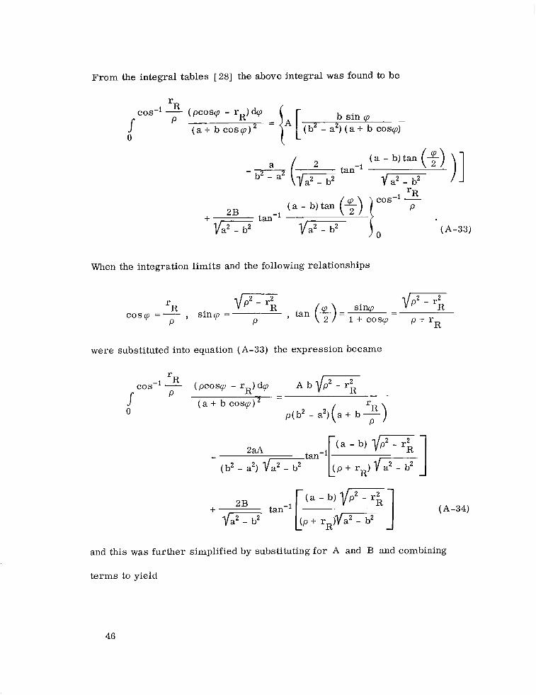
From the integral tables [28] the above integral was found to be

rRcos-' - (pcoscp - rR)dcp b sin c p . .s P ( a + b coscp) = 5.[(b'- a 2 ) ( a +b coscp)0

2B

+ v 2 - 3 tan-l

(A-33)

When the integration limits and the following relationships

were substituted into equation (A-33) the expression became

( a - b) i q- 2aA

(b2- a') tan-'[

( p + rR)m] 2B tan-' [( a - b) '/m

(A-34) ( p + rRil/a2-b2

] and this was further simplified by substituting for A and B and combining

terms to yield

46

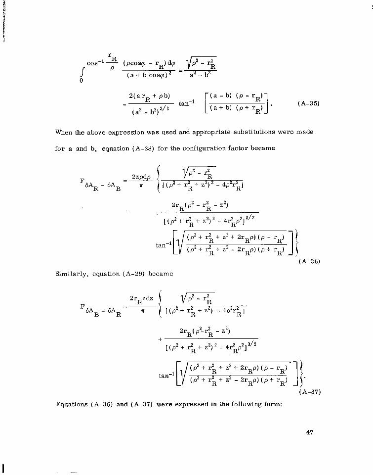
cos-'- K. (pcosq - r )dqP R -­

( a + b cosq)' a2- b2 0 s

When the above expression w a s used and appropriate substitutions were made

for a and b, equation (A-28) for the configuration factor became

2 rR ( p 2 - r2 - z2)R

(A-36)

Similarly, equation (A-29) became

(A-37)

Equations (A-36) and (A-37) were expressed in h e following form:

47

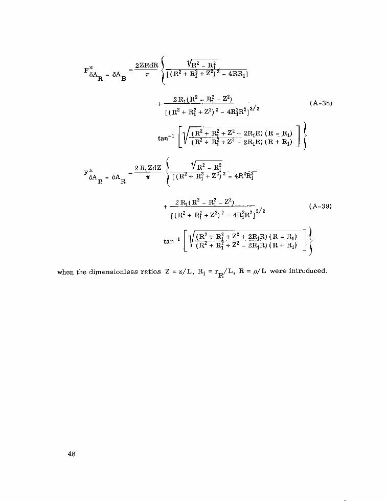
2Z RdR ViiGi--F*dAR - 6AB [ ( R 2 + R i + Z Z ) 2 - 4 R R l ]

+ 2 R1(R2 - Ri - 2’) - (A-38) [ ( R2+ Rf + 2‘) - 4RqR2]3’2

tan-’ [{( R2+ e + Z 2 + 2R,R) ( R -RL) (R2 + e + Z’ - 2R1R) ( R + Rl)

F -- 2 R1ZdZ f R 2 - @ 6AB - 6AR K [ (R’ + Rf + z‘) ’- 4R2RT

+ 2 Rl ( R2 - Rt - z2)__~- (A-39) [ ( R 2 +R?+Z2)’- 4RqR2]3/2

tan-’ (R2+ R2+ Z 2 + 2RlR) ( R - Rl)~~~

Z2 - 2R1R) ( R + Rl)

when the dimensionless ratios Z = z/L, R, = rR/L, R = p/L w e r e introduced.

48

APPENDIX B

EXPER IMENTAL EQUIPMENT

The experimental equipment consisted of the high altitude simulation

system, the data acquisition system, and the emissivity measuring device.

This equipment is government property maintained and operated by the

Propulsion and Vehicle Engineering Laboratory of the George C . Marshall

Space Flight Center.

High Al t i tude Simulat ion System

The high altitude simulation system or vacuum system consisted of the

following pr imary components: vacuum chamber; diffusion pump, ejector pump,

backing pump, and roughing pump; valves; p ressure gauges; and liquid nitrogen

storage trailer.

Vacuum Chamber. The vacuum chamber was a stainless steel cylinder

approximately 1. 83 m ( 6 feet) long and 1.22 m (4 feet) in diameter with a

dished head at each end. One of the dished heads w a s hinged for a door and the

other attached to the pumping system. The chamber environment w a s controlled

by a cooling jacket which permitted a cooling liquid such as liquid nitrogen to be

circulated through the cooling jacket and the chamber door. The door w a s a

double wal l construction connected to the jacket so that the cooling liquid

circulated through both the jacket and the door. The interior surfaces of the

49

chamber that were viewed by the tes t specimen were painted black to minimize

radiant energy reflections.

The vacuum chamber wall was designed with 3 ports that could be used

fo r viewing or for instrumentation o r for power feedthrough. For this test

the ports were used for plugs to feedthrough 64 thermocouples and 2 power

supplies.

Pumping System. The pumping system consisted of 4 pumps which could

produce a vacuum chamber minimum pressure of 1 x mm Hg. The

chamber vacuum w a s initiated by a roughing pump of large capacity. After a

rough vacuum was obtained (150 mm Hg) , the low vacuum w a s achieved and

maintained by a fractionating oil diffusion pump, an oil ejector pump, and a

rotary backing pump operating in ser ies . The pumping system was designed

and manufactured by the Consolidated Electro-dynamics Corporation for NASA/

MSFC. The following pumps were used in the system:

1. Type MCF-15000 fractionating oil diffusion pump with 0.81-m

(32-inch) diameter casing.

Operating Range: 5 x to 5 x mm Hg

Maximum Speed: 899.9 m3/min (31,779 cfm) at 3 x mm Hg

2. Kinney Type KB-I50 oil ejector pump.

Operating Range: 6 x to 4 x lo-' mm Hg

Maximum Speed: 11.53 m3/min (407 cfm) at 3 x mm Hg

50

3. Kinney Type KDH-I30 rotary oil sealed backing pump.

Free Air Displacement: 3.71 m3/min (131 cfm) at 535 rpm

Ultimate Pressure: I x IO-' mm Hg

4. Kinney Type KD-310 rotary oil sealed roughing pump.

F r e e Air Displacement: 8.81 m3/min (311 cfm) at 360 rpm

Ultimate Pressure: I x IO-' mm Hg

Valves and Gauges. The high altitude simulation system design

incorporated the necessary valves and pressure gauges to control the system.

All system valves were hand operated except the 0.81-m (32-inch) valve

between the vacuum chamber and the diffusion pump which w a s motor driven.

There were 3 types of pressure gauges used in the system: a cold cathode

ionization and a Pirani type w e r e used to monitor the chamber vacuum; a

Bourdon-tube gauge w a s used to monitor the pressure in the liquid nitrogen

storage trailer. Both the high and low vacuum gauges were products of the

Consolidated Vacuum Corporation, Rochester Division, Rochester, New York,

and w e r e of the following specifications:

I. Cold cathode ionization type

Discharge Vacuum Gauge

TYPE GPH-IOOA

Three Range Selections f rom 25 x to I x millimeters

of mercury

51

- -

2. Piran i Vacuum Gauge

TYPE 2203-04

Two range selection 2000-50 microns

The Pirani gauge was used to monitor the vacuum while the sys tem was

operating at a low vacuum and the ionization gauge w a s used to monitor the

vacuum when the system was operating at a high vacuum.

Liquid Nitrogen Storage Trailer. Liquid nitrogen w a s required fo r the_ _ -_ _ -

vacuum pumping system cold t rap and also fo r the vacuum chamber cooling

jacket. The liquid nitrogen was supplied f rom an 8165.0-kg (9-ton) capacity

liquid nitrogen storage trailer. The storage t r a i l e r w a s a self-pressurizing unit,

and was maintained at a pressure of I. 72 x IO5 - 2.07 x I O 5 N/m2 (25-30 psig)

for the test runs. Flow w a s controlled to the vacuum system by a hand valve and

the storage trailer pressure was maintained by a hand vent valve and an auto­

matic (spring-loaded) relief valve. The storage trailer w a s located outside of

the building which houses the vacuum system f o r safety reasons, and the liquid

nitrogen w a s supplied by a 2.54-cm (1-inch) diameter insulated pipe.

Data Acquisition System.- The data acquisition system consisted of 64

thermocouples, a digital recording system, and a tape controlled typewriter.

The thermocouples w e r e standard 30-gauge copper and constantan

thermocouple wiring. The thermocouples were spot welded to the specimen

and brought out of the vacuum chamber through a standard vacuum type feed-

through electrical connector. A thermocouple cold junction (ice bath) w a s

52

located adjacent to the vacuum chamber and the thermocouple outputs were

car r ied by way of a floor conduit to the recording system approximately

15.24 m (50 feet) away.

The digital recording system was a model ADRT 2100 manufactured

by the Minneapolis-Honeywell Regulator Company. The system could record

up to 100 channels of data. The system could successively sample and record

data inputs at the rate of 100 points per minute through the use of stepping

switches. A sampled input was amplified and then balanced against a precision

voltage. The balance w a s obtained by successive approximation performed by

relays pulling in successively decreasing increments of voltage. If an increment

pull.ed in w a s too large, it w a s dropped and the next smaller increment pulled in;

if the latter was too small, another smal le r increment was pulled in, etc. ,,

until the balance was achieved. A digital output w a s then punched on paper tape

along with the necessary control signals t o control a Fr iden Flexowriter. The

tape was fed through the Flexowriter control system a t each recording interval

and the data outputs w e r e typed out in millivolt units. The data acquisition

system could scan the selected number of inputs and punch the output values on

paper tape once every 1/2, I,2, 5, I O , 20, 50, o r 100 minutes, o r continuously.

F o r this series of tests, 64 thermocouples w e r e monitored and recorded

at intervals of 5 minutes f rom test beginning to completion. A l l thermocouple

millivolt outputs w e r e available for individual call up at any time. In the call

up mode, a digital reading appeared in lights by making the proper manual

selection to read the particular measurement of interest.

53

I -

The data acquisition system accuracy was dependent upon the range

selected. F o r this test series a range of 0 to 10 millivolts w a s selected and

the system accuracy in converting the thermocouple output was 10.01 millivolts

[approximately 0.22"K (0 .4"F) 1.

Emissivity Measuring Device

The emissivity of the base surface specimen w a s measured by a Gier

Dunkle-Emissivity Inspection System, Model EM 520, Geir Dunkle Instruments,

Inc. , Santa Monica, California. The emissivity inspection system measured

the emittance of an opaque surface at room temperature. The system w a s

composed of a heated radiometer connecting a flexible conduit to a carrying

case containing the power supply. When a room temperature specimen surface

covered the radiometer opening, the detector provided an output that w a s

proportional to the infrared emittance of the specimen. The output w a s

indicated on the self balancing potentiometer and this output w a s then converted

to an emissivity valve. The emissivity measurement of the base surface

specimen was made by personnel of Materials Division of Propulsion and

Vehicle Engineering Laboratory and the emissivity w a s found to be 0 . 1 3 .

54

//

APPENDIX C

I LLUSTRAT IONS

55

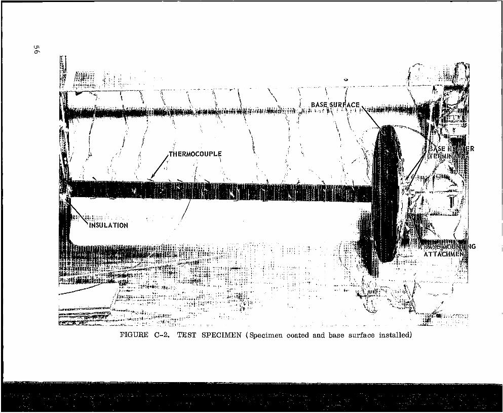
FIGURE C-2. TEST SPECIMEN (Specimen coated and base surface installed)

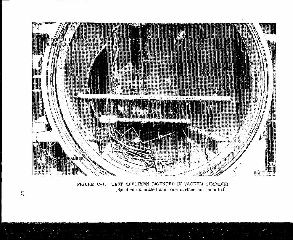
FIGURE C-I. TEST SPECIMEN MOUNTED IN VACUUM CHAMBER (Specimen uncoated and base surface not installed)

@ AMMETER

@ VOLTMETER

a VALVE

BASE t I J I I

POWER SUPPLY

ROD POWER SUPPLY

@ COLD CATHODE VACUUM GAUGE

@ PIRANA VACUUM GAUGE DIGITAL DATA DIGITALAC QU I SITI ON

SYSTEM OU T PUT

I

LIQUID NITROGEN MECHAN ICAL( STORAGE TRAILER )-I 1 1 '7'ROUGHING

MECHANICAL EJECTORBACKING PUMP

FIGURE C-3. SCHEMATIC O F TEST SETUP

1.oo

I-O2 0.95 II

0

0­-I-a E W E 3 I­4 E W L

0.9C I-

O .8!

I TEL. NO. 1 - 0 T E S T N 0 . 2

A TEST NO. 3 0 TEST NO. 4

-- T E S T ---CALCULATED

I1

0.5

LENGTH RATIO, Z = z /L

1.o

FIGURE C-4. TESTS 1-4 AND CALCULATED TEMPERATURE DISTRIBUTIONS FOR ROD WITH BASE (Uncoated)

59

--- CALCULATED

0.900 0.5

LENGTH RATIO, Z = z/L

FIGURE C-5. TESTS 5-7 AND CALCULATED TEMPERATURE DISTRIBUTIONS FOR ROD WITH BASE (Uncoated)

60

1

L

I’

1.oo

i 0.95

s0

II

0

0F 0.9C 4 e W E 3 I­4 e w = W I­

0.8:

o TEST NO.^ 0 TEST NO. 9

0.81 - 0 TEST NO. 10 A TEST NO. 11 (COATED)V TEST NO. 12 (COATED)

- 0 TEST NO. 13 (COATED) I -TEST - -CALCULATED

I

II

I

0 0.5 1.o LENGTH RATIO, Z = z /L

FIGURE C-6. TESTS 8-13 AND CALCULATED TEMPERATURE DISTRIBUTIONS FOR ROD WITH NO BASE (Coated and Uncoated)

. ,

O TESTNO. 14 A TEST NO. 15 0 TEST NO. 16 0 TEST NO. 17

CALCULATED

0.80 l - t ­0 0.5 1.o

LENGTH RATIO, Z = z / L

FIGURE C-7. TESTS 14-17 AND CALCULATED TEMPERATURE DISTRIBUTIONS FOR ROD WITH BASE (Coated)

6 2

a

360

350

340 \ L

C h

Y e ~

l­w­

\n l- 0 a tu 330 = w I­

i 320 \

\E\ ?4\ \ $ \

11

I!

'0 a 'EST NO. 12 0 TEST NO. 18 O$A T E S T NO. 19

310 -O T E S T NO. 20

0 0.5 T

1.o LENGTH RATIO, Z = z / L

FIGURE C-8. TEMPERATURE DISTRIBUTIONS FOR THERMOCOUPLE CORRECTION TEST RUNS, T('K) (Coated)

63

3

t0

t-I1 0

0' Fd W e 3 t­anf W a s W I­

1 .o LENGTH RATIO, Z = z /L

FIGURE C-9. TEMPERATURE DISTRIBUTIONS FOR THERMOCOUPLE CORRECTION TEST RUNS, 8 = T/To (Coated)

64

0.5

m 0.4F z3 U

K­O 0.3I-VU U Z0 I- 0.2U K

3-LL Z 0 0.1U \

0 10 20

DISTANCE,

-

30 40

( CENTIMETERS )z

FIGURE C-io. CONFIGURATION FACTOR OF A DIFFERENTIAL ELEMENT OF ROD VIEWING BASE FROM DISTANCE z

50

I

= 0.5

l*'P

L(ll)R1 = .026, R2 = .208 (12) R1 = R2 .I­0.85**

0 0.5

LENGTH RATIO, Z = z / L

FIGURE C-11. TEMPERATURE DISTRIBUTIONS FOR FIXED Nc AND VARIOUS R, AND R2 RATIOS (Black Surfaces)

66

1.o

0.90

0.80

0.70

0

\

(4) R1 = .l,R2 = 2.0

(5) R1 = 1.0, R 2 = 2.0

(6) R1 = .05, R2 = 1.5

(7) R, = .05, R 2 = .8

( 8 ) R1 = e l , Rg = - 8

( 9 ) R1 = .026, R2 = .416

(10) R1 = .05, R2 = .4

(11) R1 = .026, R2 = .208

(12) R1 = R2 I I --I

0.5 1.0

LENGTH RATIO, Z = z/L

FIGURE C-12. TEMPERATURE DISTRIBUTION FOR FIXED Nc AND VARIOUS R, AND R2 RATIOS (Black Surfaces)

67

I

1.o I 1

N, = 10.0

.90

.80

bo & I I

a 0'

5 .70 oc w e 3

2 oc W n s w I­

.60

(4 ) R 1 = .l,R 2 = .8

(5 ) R 1 = .026, R = .416

(6) R 1 = .OS, R 2 = . 4

.SO - (7 ) R , = .026, R 2 = . 208 .I.--&--.

0 0.5 1.0

LENGTH RATIO, Z = z L

FIGURE C-13. TEMPERATURE DISTRIBUTIONS FOR FIXED N AND VARIOUS R, AND R2 RATIOS (Black Surfaces)

C

68

1.o

I-o..+ II

a 0' F 4 E 0.5 w E z 4 E w a =E w I-

(

1

\ \ \ \

t

0.5 1.o LENGTH RATIO, Z = z/L

FIGURE C-14. SOME LIMITING CASES O F TEMPERATURE DISTRIBUTION FOR BLACK SURFACES

69

I -

1.o

0.5

0 0 5.0 10.0

CONDUCTION PARAMETER, N,

FIGURE C-15. FIN EFFICIENCY VARIATION WITH CONDUCTION PARAMETER FOR FIXED VALUES O F R, AND VARIOUS Rz RATIOS, R, = 0.026 (Black Surfaces)

Z

1.0 1 I I R, = 0.05 I

F

>-’ u z w­-U 0.5 LL LL W

-LL

0 0 5.O

CONDUCTION PARAMETER, N,

FIGURE C-16. F I N EFFICIENCY VARIATION WITH CONDUCTION PARAMETER FOR FIXED VALUES OF R, AND VARIOUS R2 RATIOS, R, = 0.05 (Black Surfaces)

10.0

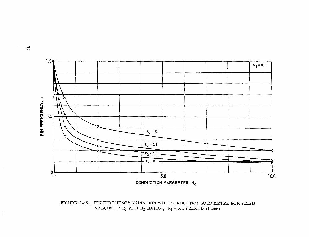
FIGURE C-17. FIN EFFICIENCY VARIATION WITH CONDUCTION PARAMETER FOR FIXED VALUES O F Rl AND R2 RATIOS, Rl = 0 . 1 (Black Surfaces)

F

CONDUCTION PARAMETER, N,

FIGURE C-18. FIN EFFICIENCY VARIATION WITH CONDUCTION PARAMETER FOR FIXED VALUES O F R, AND VARIOUS R2 RATIOS, R = 0.5 (Black Surfaces)

c

+-U z W-U 0.5 LL u. W

-z LL

0 0 5.0 10.0

CONDUCTION PARAMETER, N,

FIGURE C-19. FIN EFFICIENCY VARIATION WITH CONDUCTION PARAMETER FOR FIXED VALUES O F Rl AND VARIOUS R2 RATIOS, Rl = I.0 (Black Surfaces)

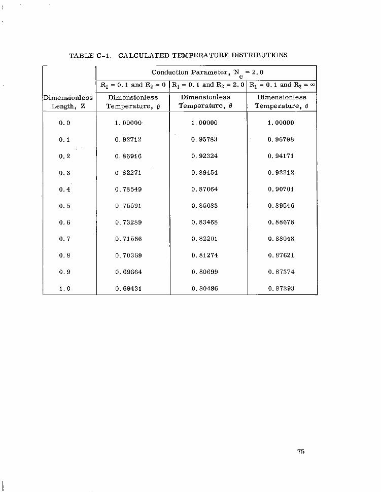
TABLE C- I , CALCULATED TEMPERATURE DISTRIBUTIONS

Conduction Parameter, 'N = 2.0 C

R i = O . I a n d R q = O Xi = 0 .1 and R2 = 2.0

)imensionless Length, Z

0.0

0 .1

0.2

0.3

0 .4

0. 5

0.6

0.7

0. 8

0 .9

1 . 0

Dimensionless Temperature, e

1.00000~

0.92712

0.86916

0.82271

0.78549

0.75591

0.73289

0.71566

0.70369

0.69664

0.69431

Dimensionless Temperature, 6

1.00000

0. 95783

0.92324

0.89454

0.87064

0.85083

0.83468

0.82201

0.81274

0.80699

0.80496

Dimensionless Temperature, 6

I.00000

0.96708

0.94171

0.92212

0.90701

0.89546

0.88678

0.88048

0.87621

0.87374

0.87293

75

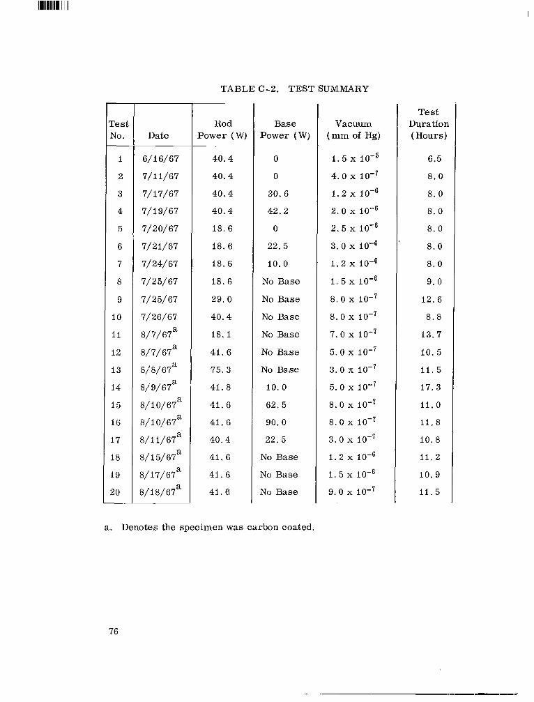
11111111111111I II II

TABLE C - 2 . TEST SUMMARY

Test rest Rod Base Vacuum Duration No. -

Date Power (W) Power (W) ( m m of Hg) (Hours)

I 6/16/67 40.4 0 1 . 5 6.5

2 7/11/67 40.4 0 4. o x 1 0 - ~ 8 . 0

3 7/ 17/ 67 40.4 30. 6 1 . 2 x 8 . 0

4 7/19/67 40.4 42.2 2 .0 x 8 . 0

5 7/ 2O/ 67 18. 6 0 2 .5 x 8 . 0

6 7/21/67 18. 6 22.5 3 . 0 x 10-6 8 . 0

7 7/24/67 18.6 10 .0 1 . 2 x 10-6 8 . 0

8 7/25/67 18. 6 No Base I . 5 x 9.0

9 7/ 25/ 67 29.0 No Base 8 . o 1 0 - ~ 12. 6

10 7/ 26/ 67 40.4 No Base 8 .0 x 8.8

11 8/7/67' 18.1 No Base 7. o x IO-' 13 .7

12 8/7/67a 41. 6 No Base 5.0 x 1 0 - ~ IO. 5

13 8/8/67a 75.3 No Base 3.0 x i l . 5

14 8/9/67a 41.8 1 0 . 0 5. o IO--' 17.3

15 8/10/67a 41. 6 62. 5 8 . 0 1 0 - ~ 11.0

16 8/ 10/67a 41.6 90.0 8. o 1 0 - ~ 11 .8

17 8/ i 1/67a 40.4 22.5 3. o x 1 0 - ~ 10.8

18 8/15/67a 41. 6 No Base 1 . 2 x 11.2

19 8/ i7/ 67a 41. 6 No Base I.5 x 10.9

20 8/ 18/67a 41.6 No Base 9. o 1 0 - ~ 11.5 -

a. Denotes the specimen was carbon coated.

76

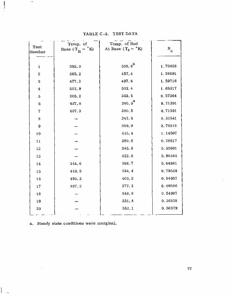
1

2

3

4

5

6

7

8

9

10

11

12

13

14

15

16

17

18

19

20

TABLE C-3. TEST DATA .. - . ~.. . ~- ___.

Temp. of Temp. of Rod Test Base ( TB - O K ) At Base (To- OK) N

C'umber _ _

393.0 508. 6a 1.70488

365.2 457.4 I . 24091

477.2 497.6 I . 59716

512.9 503.4 1.65317

305.2 353.5 0. 57264

427.8 380. 5a 0.71391

407.3 380.5 0.71391

343.5 0. 52541

389.9 0.76818

445.4 1.14507

280.6 0.28617

345.8 0. 53601

- 423.6 0.98 544

344.6 368.7 0.64961

449.9 394.4 0.79549

490.2 403.2 0.84957

367.2 377.2 0. 69586

348.8 0. 54987

351.4 0. 56258

- 352, l 0. 56579 - . - . .____

a. Steady state conditions w e r e marginal.

77

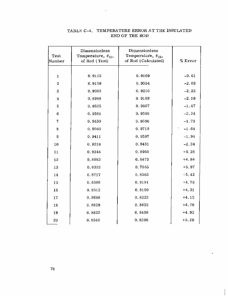
TABLE C-4. TEMPERATURE ERROR AT THE INSULATED END O F THE ROD

Dimensionless Temperature, O i l ,

of Rod (Test)

0.9113

0.9159

0.9003

0.8988

0.9525

0.9381

0.9430

0.9560

0. 9411

0. 9210

0.9344

0.8883

0.8322

0.8717

0.8568

0.8512

0.8668

0.8829

0.8822

0.8840

Dimensionless Temperature, 8ii, of Rod (Calculated)

0.9169

0.9354

0.9210

0. 9189

0. 9667

0. 9596

0. 9596

0. 9719

0.9597

0. 9431

0.8960

0.8473

0.7865

0.8363

0. 8181

0.8160

0.8323

0.8433

0.8408

0.8396

% E r r o r

-0.61

-2.09

-2.25

-2.19

-1.47

-2.24

-1.73

-1.64

-1.94

-2.34

+4.28

+4.84

+5.97

+5.42

+4.73

+4.31

+4.15

+4.70

+4.92

+5.29

78

L IST OF REFERENCES

I . Jacob, Max: Heat Transfer , Vol. I. John Wiley and Sons, Inc. , New York, 1957, pp. 97 and 207-243.

2. Langmuir, Irving: Heat Conductivity of Tungsten at High Tempera­tu re s and the Wiedmann-Franz-Lorenz Relation, Physical Review, Vol. 7, NO. I , 1916, pp. 151-152.

3. Langmuir , Irving, and Taylor, John Bradshaw: The Heat Conductivity of Tungsten and the Cooling Effects of Leads Upon Filaments at Low Temperatures. Physical. ~-Review, Vol. 50, 1936, pp. 68-87.

4. Worthing, A. G.: Temperature Distribution in a n Incandescent Lamp ~. .Filament in the Neighborhood of a Cooling Junction. Physical Review,

Vol. 4, No. 6, 1916, pp. 524-534.

5. Worthing, A. G., and Holiday, D. : Heat. John Wiley and Sons, Inc. , New York, 1948, p. 171.

6. Stead, G. : The Short Tungsten Filament as a Source of Light and Electrons. Journal of Instn. Elect. Engr s . , Vol. 58, 1920, pp.- .-- .- ­

107-117.

7. Bush, V. , and Gould, King E . : Temperature Distribution Along a ._Filament. Physical Review, Vol. 29, 1927, pp. 337-345.

8. Baerwald, H. G. : The Distribution of Temperature in a Cylindrical Conductor Electrically Heated in Vacuo. Phil. Mag. , Vol. 21, No. 141, 1936, pp. 641-648.

9. Jain, S. C. , and Krishnan, Sir K. S. : The Distribution of Temperature Along a Thin Rod Electrically Heated in Vacuo. Part I, Theoretical Proceedings of Royal Society, Ser ies A , Vol. 222, 1954, pp. 167-180; Part 11, Vol. 225, 1954, pp. 1-7; Part 111, Vol. 225, 1954, pp. 7-18; Part IVYVol. 225, 1954, pp. 19-32; Part V, Vol. 227, 1955, pp. 141­154; Part VI, Vol. 229, 1955, pp. 439-444.

I O . Shouman, A. R. : Nonlinear Heat Transfer and Temperature Distribu­tion Through Fins and Electric Filaments of Arbi t rary Geometry with Temperature-Dependent Propert ies and Heat Generation. National Aeronautics and Space Administration, Washington, D. C., TN D-4257, January 1968, pp. 1-24.

. 79

LIST OF REFERENCES (Continued)

11. Lieblein,, Seymour: Analysis of Temperature Distribution and Radiant Heat Transfer Along a Rectangular Fin of Constant Thickness. National Aeronautics and Space Administration, Washington, D. C. , TN D-196, November 1959, pp. 1-18.

12. Chambers, R. L. and SOmers, E. V. : Radiation Fin Efficiency f o r One-Dimensional Heat Flow in a Circular Fin. Trans. ASME, Vol. 81, 1959, pp. 327-329.

13. Tatom, J. W. : Steady-State J3ehavior of Extended Surfaces in Space. ARS Journal, Vol. 30, 1960, p. 118.

14. Callinan, J. P. , and Berggren, W. P. : Some Radiator Design Cri ter ia for Space Vehicles. Trans. ASME, Series C, Vol. 81, 1950, pp. 237-244.

15. Baptas, J. G. , and Sellers, W. H. : Radiation Fin Effectiveness. Trans. ASME, Series Cy Vol. 82, 1960, pp. 73-75.

16. Sparrow, E. M. , Eckert, E. R. G. , and Irvine, T. F., Jr.: Analytical Formulation fo r Radiating F ins with Mutwd Irradiation. ARS Journal, Vol. 30, 1960, pp. 644-646.

17. Sparrow, E. M., Eckert, E. R. G., and Irvine, T: F., Jr. : The Effectiveness of Radiating Fins with Mutual Irradiation. Journal of the Aerospace Sciences, Vol. 28, 1961, pp. 763-772.

18. Karlekar, E. V. , and Chao, B. T. : Mass Minimization of Radiating Trapezoidal Fins with Negligible Base Cylinder Interaction. Int. J. of Heat and Mass Transfer, Vol. 6 , 1963, pp. 33-48.

19. Hering, R. G. : Radiative Heat Exchange Between Conducting Plates with Specular Reflection. Trans. ASME, Series C y Vol. 88, 1966, pp. 29-36.

20. Sparrow, E. M. , and Eckert, E. R. G. : Radiant Interaction Between Fin and Base Surfaces. Trans. ASME, Series C, Vol. 84, 1962, pp. 12-18.

21. Sarabia, M. ' F. , and Hitchcock, J. E. : Heat Transfer from Gray Fin-Tube Radiators. Trans. ASME, Series C y Vol. 88, 1966, pp. 338-340.

80

L IST OF REFERENCES (Concluded)

22. Hwang-Bo, H. : Optimization of Some Radiators with Fins and _---Involute Reflectors. Trans. ASME, Series C, Vol. 89, 1967,

pp. 99-102.

23. Sparrow, E. M., Miller, G. B., and Jonsson, V. K. : Radiating Effectiveness of Annular-Finned Space Radiators, Including Mutual

- .Irradiation Between Radiator Elements. Journal of the Aerospace Sciences, Vol. 29, No. 1, 1962, pp. 1291-1298.

24. Gordon, G. D. : Measurement of Ratio of Absorptivity of Sunlight to Thermal Emissivity. The Review of_______Scientific Instruments, Vol. 31, No. 11, 1960, p. 1207.

25. Schnieder, P. J. : Conduction Heat Transfer . Addison-Wesley Pub­lishing Company, Inc. , Reading, Massachusetts, 1957, pp. 3 and 4.

26. Sparrow, E. M., and Cess , R. D. : Radiation Heat Transfer . Brooks/ Cole Publishing Company, Belmont, 'California, 1966, pp. 86-90, pp. 113-126, and pp. 170-176.

27. Herriot , J. G. : Methods of Mathematical Analysis and Computation. John Wiley and Sons, Inc. , New York, 1963, pp. 23-24.

28. Dwight, H. B.: Tables of Integrals and Other Mathematical Data. The Macmillan Company, New York, 1957.

NASA-Langley, 1970 - 33 M362 81

AERONAUTICSNATIONAL AND SPACE ADMINISTRATION WASHINGTON,D. C. 20546

OFFICIAL BUSINESS FIRST CLASS MAIL

POSTAGE AND FEES PAID NATIONAL AERONAUTICS AN

SPACE ADMINISTRATION

r I

POSThfASTER:

"The nesorzrrittical and SQACe ctctit'ities of the Uizited States shall be coizdilcted so lis to contribnte . . . t o the expnizsion of hzoiinn knoiul­edge of pheizoniem iit the ntiiiosphese and spnce. The Adiiiimstsntion shnll psoiride for the widest pacticnble nrzd appropsiate disseriiirtntion of iiiforiiintiov. coizceriziag its nctiirities nizd the w s d t s theseof."

-NATIONALAERONAIJTICSA N D SPACEACT OF 19%

If Undeliverable (Section 15s Postal Manual) Do Not Returr

NASA SCIENTIFIC AND TECHNICAL PUBLICATIONS

TECHNICAL REPORTS: Scientific and technical information considered important, complete, and a lasting contribution to existing knowledge.

TECHNICAL NOTES: Information less broad in scope but nevertheless of importance as a contribution to existing knowledge.

TECHNICAL MEMORANDUMS: Information receiving limited distribution because of preliminary data, security classifica­tion, or other reasons.

CONTRACTOR REPORTS: Scientific and technical inforniati?m generated under a NASA contract or grant and considered an important contribution to existing knowledge.

TECHNICAL TRANSLATIONS: Information published in a foreign language considered to merit NASA distribution in English.

SPECIAL PUBLICATIONS: Information derived from or of value to NASA activities. Publications include conference proceedings, monographs, data compilations, handbooks, sourcebooks, and special bibliographies.

TECHNOLOGY UTILIZATION PUBLICATIONS: Information on technology used by NASA that may be of particular interest in commercial and other non-aerospace applications. Publications include Tech Briefs, Technology Utilization Reports and Notes, and Technology Surveys.

Details on the availability of these publications may be obtained from:

SCIENTIFIC AND TECHNICAL INFORMATION DIVISION

NATIONA L AERO NAUT1C S AN D SPACE ADM INISTRATI0N Washington, D.C. 20546