ItifA Til V '''1 NR)R IM A-JLJ NASA TECHNICAL

MEMORANDUM Co

C

>

I-

CALCULATION PROCEDURE FOR TRANSIENT

HEAT TRANSFER TO A COOLED PLATE

IN A HEATED STREAM WHOSE TEMPERATURE

VARIES ARBITRARILY WITH TIME

James Sucec

Lewis Research Center

Cleveland, Ohio 44135

0UJTIQ

'Ji

NATIONAL AERONAUTICS AND SPACE ADMINISTRATION WASHINGTON, D. C. • JUNE 1915

https://ntrs.nasa.gov/search.jsp?R=19750017023 2018-06-10T10:55:43+00:00Z

1. Report No. 2. Government Accession No. 3. Recipient's Catalog No.

NASA TMX-3238 4. Title and Subtitle CALCULATION PROCEDURE FOR TRANSIENT 5. Report Date

HEAT TRANSFER TO A COOLED PLATE IN A HEATED June 1975 STREAM WHOSE TEMPERATURE VARIES ARBITRARILY 6. PerformIng Organization Code

7. Author(s) 8. Performing Organization Report No.

James Sucec E-8217 10. Work Unit No.

505-04 ________________________________________________________________________________ 9. Performing Organization Name and Address

Lewis Research Center11. Contract or Grant No.

National Aeronautics and Space Administration Cleveland, Ohio 44135

13. Type of Report and Period Covered

Technical Memorandum 12. Sponsoring Agency Name and Address

National Aeronautics and Space Administration14. Sponsoring Agency Code

Washington, D.C. 20546

15. Supplementary Notes

16. Abstract

Solutions for the surface temperature and surface heat flux are found for laminar, constant property, slug flow over a plate, convectively cooled from below, when the temperature of the fluid over the plate varies arbitrarily with time at the plate leading edge. A simple tech-nique is presented for handling arbitrary fluid temperature variation with time by approximating it by a sequence of ramps or steps for which exact analytical solutions are available.

17. Key Words (Suggested by Author(s)) 18. Distribution Statement

Transient convection Unclassified - unlimited Transient STAR category 34 (rev.)

19. Security Classif. (of this report) 20. Security Classif. (of this page) 21. No. of Pages 22. Price

Unclassified Unclassified 24 $3. 25

* For sale by the National Technical Information Service, Springfield, Virginia 22151

CALCULATION PROCEDURE FOR TRANSIENT HEAT TRANSFER TO A COOLED

PLATE IN A HEATED STREAM WHOSE TEMPERATURE

VARIES ARBITRARILY WITH TIME

by James Sucec*

Lewis Research Center

SUMMARY

Solutions for the surface temperature and surface heat flux are found for a flat plate, convectively cooled from below, when the temperature of a fluid flowing over it in a laminar, constant property, slug-flow fashion is varying arbitrarily with time. A specific solution is given for the important case, from the practical standpoint, of the fluid temperature at the plate leading edge varying in a linear fashion with time between two specified temperatures. The solution to the linear case, after being properly gen-eralized, also serves as the basis for the rapid, approximate treatment of transients induced by any fluid temperature variation with time. This is done by approximating the actual fluid temperature variation at the plate leading edge by a series of ramps or steps, thus.giving relatively simple functions for the surface heat flux and temperature responses. Several example cases are worked to illustrate the application of the k_nown solutions for the step and the ramp to more general fluid-inlet temperature variations. Finally, a limited comparison with some experimental data is made.

INTRODUCTION

This work predicts the unsteady surface heat flux and temperature of a plate when the fluid passing over it has its temperature at the plate leading edge varying arbitrarily with time. As such, it represents an extension and generalization of the work reported previously in reference 1.

* Associate Professor of Mechanical Engineering, University of Maine, Orono, Maine; NASA & ASEE Summer Faculty Fellow at the Lewis Research Center in 1972 and 1973.

Transients in a plate are dften induced by a controlled change with time of the tem-perature of the fluid flowing over the plate as opposed to the case of a controlled change in the plate temperature or heat flux. When the fluid induces the transient, which the plate must then respond to, the temperature distributions in the fluid and the plate are mutually coupled, and one has a so-called "conjugate" problem. This plate could be an idealization of a rocket motor wall during startup, a nuclear reactor component, a re-cuperative heat exchanger during startup and shutdown, or a regenerative heat ex-changer either in the transient unsteady domain or, the ultimate periodic unsteady time domain. The primary physical motivation for the work, however, is the transient in-duced in gas turbine blades and vanes as a result of startup, shutdown, or changes in the steady-state power level of an already operating engine.

A review of much of the previous associated work in transient, forced-convection heat transfer is given in reference 1. The most pertinent of the works reviewed are references 2 and 3, in which heat transfer at a stagnation point due to a sudden change in free-stream temperature, with the wall temperature field mutually coupled to the fluid temperature field, is solved using approximate integral techniques. In reference 4 the dynamic response of thin heat exchanger walls is treated by the Laplace transforma-tion under the assumption of quasi-steady conditions with a constant surface coefficient of heat transfer. Reference 5 treats the case of a transient in a pipe wall (infinite thick-ness) due to a change in the fluid inlet temperature but restricts the analysis to quasi-steady conditions and to the use of a constant surface coefficient of heat transfer between the wall and the fluid. One of the problems dealt with in reference 6 is the unsteady heat transfer to and temperature of a sphere when it is suddenly subjected to a fluid with a different temperature flowing in a Stokesian manner about the sphere. The entire sphere is lumped in the space coordinates, and its temperature is coupled to that of the fluid. A Laplace transformation of the governing equations, followed by numerical in-version, yields the heat-transfer response curves for the sphere. Quasi-steady solu-tions are also presented, and their range of validity discussed. In reference 7 a fluid whose temperature is varying sinusoidally with time enters a duct in a slug flow fashion, that is, with a uniform velocity distribution. The duct walls are thin plates, insulated on their outside surfaces and interacting with the fluid on their inside surfaces. After neglecting axial conduction in plate and fluid, lumping the plate temperature trans-versely, and using the energy balance equation on the plate as a fluid boundary condition, a technique somewhat like the method of complex temperature (ref. 8) is used to effect a solution by separation of variables. Reference 9 also deals with the case of a sinus-oidal fluid temperature at the entrance of a duct, but with nonparticipating walls.

The unsteady surface heat flux and temperature of cooled gas turbine blades and vanes, caused by a turbine inlet temperature varying in some prescribed, though com-pletely general, fashion with time, is the subject of the present investigation. Using a

2

number of idealizations, a solution to the problem is found which allows study of the general heat transfer behavior for laminar flow over blades and vanes (as well as any of the applications previously mentioned) during this type of transient.

ANALYSIS

Arbitrary Variation of Fluid Temperature at x 0 with Time

Consider the plate of, thickness b (fig. 1) with its bottom surface subject to a cool-• ant at constant temperature T and with a constant surface coefficient of heat transfer hc between the coolant and the plate bottom. (Symbols are defined in appendix A.) The fluid passing over the plate has its temperature at x = 0, the plate leading edge, chang-ing with time t in some prescribed fashion (fig. 2). For t ^ 0, T = Tc• The response of the surface heat flux and temperature to this arbitrary variation of fluid temperature at x = 0 is required.

As in reference 1 the flow is considered to be laminar, low-speed, constant pro-perty, two-dimensional planar, and of the thin thermal boundary layer type. In addi-tion, a steady slug flow velocity profile is used, plate and fluid axial conduction is neglected, and the plate temperature is to depend on only x and t(i. e., the plate's temperature is lumped in the y direction). In attempting to find the response to an arbitrary variation with time of the fluid temperature at x = 0, one first seeks the solu-tion for a step change in the fluid temperature which then, by virtue of the linearity of the governing equations and boundary conditions, can be used with Duhamel's theorem to yield the more general result. The mathematical statement of the problem for a step change in fluid temperature from T to T0 is

aT T

ay2

at t=Ox>0, y>0T=T at x=Ot>O, y>OT=T 0 as y— oo t>0, x>0 T remains finite. The exact analytical solution to this equation, subject to the side conditions shown, was found in reference 1 using double Laplace transformations. The solution is now presented in terms of the more convenient variable (for use with Duhamel's theorem) cr = T - Tc with a0 = T0 - T:

a = a0u(r - 1) (erf (Y) + e22 {erf [c(r - 1) + + y] - erf (i + Y)}) (1)

3

where the unit step function is

10 for T<1 u(r- 1) = (2)

+l for i-^l

• The appearance of the unit step function is the mathematical manifestation of the physics of the plane wave phenomenon, namely, that at position x the plate cannot re-spond to what has happened to the fluid at x = 0 and time = t until the fluid, that was at x = 0 at time = t, reaches the position x. The nondimensional variables appearing in equation (1) are defined in reference 1 and repeated here for convenience.

u t=

ç = PfC, f1 Y______

x 2 afX kf u 2PwCp, b

Using Duhamel's theorem (reL 8) along with equation (1) when a 0 = 1 and j3 = a gives the transient temperature distribution within the moving fluid for arbitrary variation of the fluid temperature at the plate leading edge with time as

J

I(i, E, Y, T -daø(X) dX

0dA

where X is a dummy variable for the nondimensional time i-.

Since the plate surface temperature is usually of primary interest, Y is set equal to zero and the function /3 is inserted to yield the result for the plate surface tempera-ture when the fluid temperature variation is arbitrary, namely,

2Jda

aw = e • {erf [€( - A) + - erf x=0 dA (5)

0dA

where cp = T - 1. The treatment of the unit step function during the integration is shown in appendix B. Defining a surface heat flux parameter F as

I (4)

4

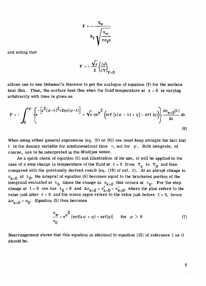
F=

kflrafX

and noting that

F-( 2

allows one to use Duhamel's theorem to get the analogue of equation (5) for the surface heat flux. Thus, the surface heat flux when the fluid temperature at x = 0 is varying arbitrarily with time is given as

- dcrø(X)dA f [€2(x)2+2€(x)]

(erf [€( - X) + - erf ()) F=- e

+ (6) 0

When using either general expression (eq. (5) or (6)) one must keep straight the fact that A is the dummy variable for nondimensional time 'r, not for ço. Both integrals, of course, are to be interpreted in the Stieltjes sense.

As a quick check of equation (5) and illustration of its use, it will be applied to the case of a step change in temperature of the fluid at t = 0 from Tc to T0 and then compared with the previously derived result (eq. (15) of ref. 1). At an abrupt change in

at A 0, the integral of equation (5) becomes equal to the bracketed portion of the integrand evaluated at times the change in Ux=O that occurs at X. For the step change at t = 0 one has A 0 = 0 and OxO = - where the plus refers to the value just after t = 0 and the minus signs refers to the value just before t = 0, hence

0x=O = Equation (5) thus becomes

2 = e erf(€co + i) - erf(j)J for -p > 0 (7)

a0

Rearrangement shows that this equation is identical to equation (15) of reference 1 as it should be.

Solutions for Generalized Step and Ramp in Fluid Temperature at x = 0

In general, for an arbitrary T 0 as a function of time, the integrals of equations (5) and (6) often cannot be found analytically. But T0 can be approximated by a se-quence of steps and ramps to any desired accuracy, and equations (5) and (6) do admit analytical, relatively simple solution functions for both the step change and the ramp change in fluid temperature at x = 0. Hence, response functions for any arbitrary fluid temperature at x = 0 can be constructed, approximately, by the proper combination of the response functions for the generalized step and generalized ramp as will be ex-plained later.

For the response to a generalized step in fluid temperature where T 0 changes from T 0 to T 0 at time t, which corresponds to Ti = A, equations (5) and (6) yield the solutions (from ref. 10)

erf [€( - T ) + - erf (ij)} (8)

for 'p > Ti and

F = + e12 (erf[c( - T ) + - erf ()) (9)

for 'p > Ti, where = T 0 - T 0 the subscript i on the Ow and F refers to the time at which the step occurs, and the superscript s indicates that these are re-sponses to a step as opposed to a ramp.

The generalized ramp, in which T 0 changes in a linear fashion from T at time to T at time t, is depicted in the portion of figure 2 bounded by the dashed refer-

ence lines. The response functions for this case are important not only for their role when the fluid temperature varies arbitrarily, but also because often during a startup, shutdown, acceleration, or deceleration of a gas turbine engine, the turbine-inlet tern-perature, as a first approximation, can be represented as varying linearly with time. The equation of the generalized ramp is

T 0 = T + (T - T)() t

t t (10)

Using this in equations (5) and (6) leads to the following response functions for the ramp (as presented in ref. 10).

6

________ .1 (T. - T\e112 =) - 1€ ( ço - r1 ) eric (ij) + i eric [€ ( - T) +

- i 1 erfc ( )}

- Ti,! €(11)

for Ti < q' <

(T_- T\

{E(T. - r.) erfc () + i 1 eric [€( - T) +- i 1 erfc [€( -

+

1 \T_T) € 1

(12) for co^.T)

(T. - T eli2 ( {erf () - en [€( - r ) + - €( - T) eric (1)

Fr =

I ______ \T_Tjj e 2

+ erfc (ii) - i 1 erfc [€( - T) +(13)

for T<co<Tj and

Ff = - Ti)

( erf €( - Tj) +

- erf - T) + li}- li € (Tj - Ti) eric ()

Tj_Ti €

+ erfc [€( - + i1 - i' eric [€( - + i) (14)

for çü ^ r. The subscript i denotes the time at which the ramp begins, the super-script r is the response due to the ramp, the prime on the r indicates the validity of the expression in the ço domain given by T < q' < Tj and i' eric (ii) is the first re-peated integral of the error function and is defined and tabulated in reference 11. (A representative portion of the details of the integrations of eqs. (5) and (6) subject to eq. (10) is given in appendix C)

Solutions Obtained by Combining Steps and Ramps

Equations (8), (9), and (11) to (14), when appropriately combined, give the transient surface temperature and heat flux due to a preribed fluid temperature variation at

7

x = 0, when it is approximated by a series of steps and/or ramps. As an illustration, consider the fluid temperature variation at x = 0 shown as a solid line in figure 3. Also shown in figure 3 are three dashed lines that form a step and two ramps which ap-proximate fairly closely the actual fluid temperatures as a function of time. (No dashed line is shown beyond time t 3 because it coincides with the solid line there.) Hence, the flux at time t, say, when t 1 <t <t2 is given by the following sum:

F = (Eq. (9) with T = 0 and = T1 - Tc) + (Eq. (14) with Ti = 0, T T1, and T

- T1 = T2 - T 1 ) + (Eq. (13) with Ti = r, T = T2 , and T - T1 = T0 - T2)

The details of the procedure for the case depicted in figure 3 are illustrated in ap-pendix D.

RESULTS AND DISCUSSION

Transient Due To Change From One Steady State Operating Level to Another

In the analysis section and appendix D, the procedure for handling the more general cases of fluid temperature variation with time are discussed, and the example shown in figure 3 is worked in some detail. Now consider the case depicted in figure 4, where

T 0 = T 1 for t < 0 and then linearly increases to T 0 at time t = t 1 and is held at T0 thereafter.

The response of the surface temperature and flux consists of the proper combining of equations (8), (9), and (ii) to (14). The contribution to o and F for t < 0 can be considered to have resulted from a step change in fluid temperature from Tc to T 1 a long time ago. Hence, this portion of the response is given by equations (8) and (9) as ço (interpreted here as the time elapsed since the step function changed Tx0 from Tc to T 1 ) goes to infinity. Thus, the contributions to the wall temperature and flux for t> 0, but due to the history of the fluid before t = 0, are

2 = (T1 - Tc)e erfc (i)

(15)

and

2 F = -(T 1 - T ) I ie erfc (ii) (16)

For 0 <t <t 1 the right hand side of equation (11) would be added to equation (15) and the right hand side of equation (13) would be added to equation (16) with T set to zero

8

and = r1 with T - T = T0 - T 1 . These sums give the responses in the time do-

main between 0 and t 1 . For t > t 1 the right hand sides of equations (12) and (14) would be added to equations (15) and (16), respectively, to yield surface temperature and

heat flux for values of time t > t 1 . The solution is now complete. Division of the final

equations for the aw and F by T 0 - Tc to yield (Tw - T )/(To - Tc) and re-

spectively, gives, as the solution functions for the surface temperature and surface heat flux, for the case shown in figure 4, the following:

Tw - T (Ti_-_Tc\2

T O Tc \ToTcJ

' 2 / 1 0 - T1\eIl

erfc (i) + I-- Tel En

[E q, erfc (77) + i 1 erfc (€çü + 77)

- i 1 erfc (77)]

for 0 S :S

TwTc /T 1 -T \ 2 /T0Ti\e772 c \e77 erfc (i7)+f

T0 - T T0 - T) \T0 - Tc)ET1 {€ erfc () + i 1 erfc (€ +

- i 1 erfc [€( - T1) +

for ço ^T1

(18)

(19)

/T 1 -T\ ,-.- 2

\T0- c/erfc

(o Tie772

\T0 - T, €n1! [erf (€ço + 11) - erf

+ erfc (ij) + erfc (€ + 77) - i 1 erfc (7)]}

for 0 T, and

=(--- Tc\77e772 erfc/T0 - T1\

Ierf (€ + 77)- erf[E( -

(i)+( 1 T 0 - Tc) \T0 - T el ET 1 2

+ + i€r1 erfc (ij) + erfc [E + 71] - i 1 erfc [€( - r1 ) +

for çOT1.

(20)

(21)

9

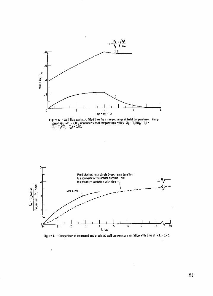
Equations (18) to (21) are plotted in figures 5 and 6 for a value of CT 1 = 2. 00 and for (T1 - T )/(To - T ) = (T 0 - T1)/(T0 - Tc) = 0.50. The CT1 value is (as noted in ref. 10) a measure of the steepness of the ramp that takes T 0 from T 1 at t = 0 to T 0 at t = t 1 . The curves in figures 5 and 6 are plotted for two values of ij: 1J = 0 cor-responding to an insulated plate (not cooled) and i = 1 corresponding to a rather well cooled plate. The plate, of course, does not respond to the change in the fluid temper-ature at T = 0 until T = 1, hence, the reason for plotting the time parameter as E(T - 1). It is seen from figure 5 that, for both cases, i = 0 and i = 1, the wall tem-perature increases monotonically from the original steady-state temperature to the final steady-state temperature corresponding to the new fluid temperature at x = 0, T 0 . In figure 6 the surface heat flux continually increases until the displaced time (T - 1) at which the fluid temperature at x = 0 ceases its variation with time. Beyond this time the surface heat flux decays to its final steady state value.

Comparison With Data

A comparison of the predictions of the theory presented in this work with some ex-perimental data would be desirable. However, only an extremely rough comparison could be made because of incomplete data and, in particular, data from a case that did not satisfy the major restrictions of the idealized model. The measured data was from an air cooled vane (describc in ref. 12) during an acceleration in a laminar flow region of the vane surface, Because of a nonslug velocity profile, axial and spanwise conduc-tion, transverse temperature gradients, and x-dependent hc in the experiment, one would not expect even the initial or final steady-state nondimensional temperatures to be predicted well. Hence, an attempt was made to over-ride some of these effects by com-paring (Tw - Tc, initial (Tw, initial - T initial since this parameter is unity at the start of the acceleration for both the measured data and the theoretical solution. The subscript "initial" pertains to values of T and T just before the acceleration. During the transient in the turbine-inlet temperature, which was approximated by a single ramp for the analysis, one also encounters time varying T , hc and u,,. These parameters are assumed constant and are, in addition to the aforementioned effects, therefore not taken into proper account in the analysis. Also present in the experiment was extreme property variation and a variable thickness wall. To make a rough comparison, arithmetic averages of T, u,,, , and the fluid properties were used along with the value of h at the end of the acceleration. Considering the vast differ-ences between the experimental conditions and the constraints on the analytical model, the agreement between theory and experiment is at least encouraging. In figure 7 the measured wall temperature response curve is plotted against time at x/L = 0. 40 for

10

an acceleration in which the turbine-inlet temperature changes from 922 to 1644 K (12000 to 2500° F). Also plotted is the analytical curve, which comes from equations (18) and (19). The qualitative behavior of the nondimensional temperature excess ratio just referred to was predicted by the theory. The percentage error between the two was about 26 percent at low times and about 12 percent at the final steady state. The mani-fold differences between the theoretical model and the experiment preclude any conclu-sive explanation of these percent differences. However, a rough calculation indicates that the neglect of transverse temperature differences (the lumped in the y direction assumption) is an important difference between the theory and experiment.

SUMMARY OF RESULTS

Expressions for the surface temperature and surface heat flux are found for a plate, convectively cooled from below, while the temperature of a fluid passing over the top of the plate is changed arbitrarily with time at the plate leading edge.

1. Simple, easy to use functions were presented that allow a solution to the problem of fluid temperature varying arbitrarily with time by approximating the arbitrary fluid temperature variation by a sequence of ramps or steps.

2. The mechanics of properly combining these functions to yield plate temperature

and heat flux is demonstrated by means of examples. 3. Equations are given for the important case of a ramp in fluid temperature at

x = 0 causing T0 to change from temperature T 1 at time t = 0 to temperature T0

at t = t 1 and held at T0 thereafter. 4. A limited comparison of the predictions of the idealized model with experimental

results was made for a case that did not satisfy many of the restrictions of the model. This yielded a rough qualitative similarity of the predictions and the data.

Lewis Research Center, National Aeronautics and Space Administration,

Cleveland, Ohio, March 4, 1975, 505- 04.

11

APPENDIX A

SYMBOLS

b plate thickness

C constant-pressure specific heat p

F surface heat flux parameter,I-;--

1TX

F surface heat flux response function defined by eq. (14)

F ' surface heat flux response function defined by eq. (13)

F5 surface heat flux response function defined by eq. (9)

h coolant-side surface coefficient of heat transfer

i 1 erfc (z) first repeated integral of error function, erfc (z') dz'

kf thermal conductivity of fluid flowing over upper surface of plate

instantaneous nondimensional surface heat flux

instantaneous surface heat flux

T temperature

T coolant temperature

Tø instantaneous fluid temperature at x = 0

t time

- 1) unit step function, equal to 0 for 7 < 1, and to +1 for ^ 1

u free-stream velocity

v variable defined by eq. (C5)

x space coordinate along plate

Y nondimensional y coordinate defined in eqs. (3)

y space coordinate perpendicular to plate

af thermal diffusivity of fluid flowing over plate

value of a when a0 = 1

nondimensional variable defined in eqs. (3)

p density

12

X dummy variable for time

a temperature difference, T - T ar temperature response function defined by eq. (12) Wi

temperature response function defined by eq. (ii)

temperature response function defined by eq. (8) WI

nondimensional variable defined in eqs. (3)

T nondimensional time defined in eqs. (3)

T i nondimensional duration of ramp that begins at t = 0

'P shifted nondimensional time, r - 1

Subscripts:

f properties of fluid flowing over plate

i index

j index

w wall

0 ultimate steady-state fluid condition at x 0

free-stream conditions

Superscripts:

r response to ramp after it has ended

rt response to ramp before it has ended

s response to step in fluid temperature at x = 0

13

APPENDIX B

DEVELOPMENT OF EQUATION (5)

To find for an arbitrary variation of fluid temperature at x = 0, against time, when the wall is initially at T, Y is set equal to 0 in equation (4), and i3 is given by the right side of equation (1) with Y = 0, a = +1, and T replaced by T - A. Doing this yields

2T

= e f u(T - A - 1) {erf [€(r - A - 1) + - erfda0(A) dA (Bi).

0

However, u(T - A - 1) = +1 only for T - A - 1 ^ 0 by definition of the unit step function; hence, A - 1. Thus, since A is the integration variable and values of A > T - 1 lead to a zero integral, this is taken into account by making the upper limit equal to

- 1, which has been defined as q. This change obviates the need for explicit appear-ance of the unit step function in equation (Bi) and thus it becomes

o•w =

e' .J °

erf [€( - A) +

- erf } da0(A)

(B2)

which is equation (5).

14

APPENDIX C

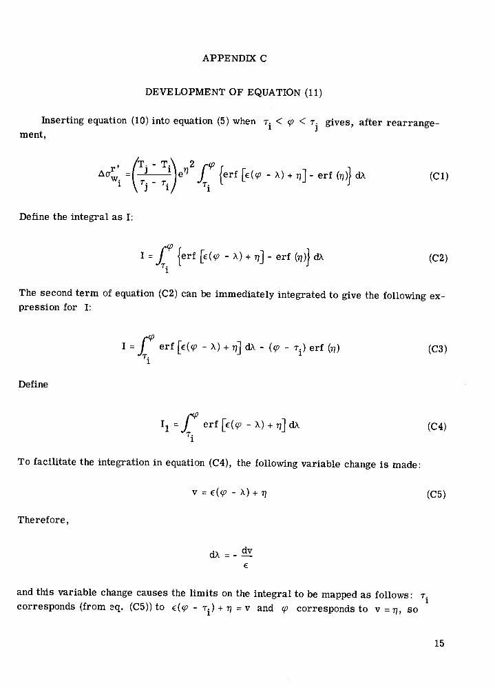
DE-VELOPMENT OF EQUATION (11)

Inserting equation (10) into equation (5) when Ti < 'p <T gives, after rearrange-ment,

r' (T -_Ti\e2f erf [€('p - X) ^ ]- en ()} dA (Cl) w '\Tj - Tj)

Define the integral as I:

i=f 'p Ierf[E(X)+]erf(7J)}dX (C2)

The second term of equation (C2) can be immediately integrated to give the following ex-pression for I:

I =

erf [€('p - A) + dA - ( 'p - T) erf (ij) (C3)

Define

i =f erf [€('p - A) + dA (C4)

To facilitate the integration in equation (C4), the following variable change is made:

v = €('p - A) + (C5)

Therefore,

dA = -€

and this variable change causes the limits on the integral to be mapped as follows: Ti corresponds (from q. (C5)) to €('p - T) + = v and 'p corresponds to v = i, so

equation (C4) becomes

1

erf (v) dv (C6) '1 = - f -erf (v) dv

€ E(p

Adding and subtracting unity to the integral of equation (C6), noting that 1 - erf (v) erfc (v), and integrating the constant term gives

1

= ço - - -J erfc (v) dv (C7) €71

Rearranging gives

= - T. - Ij erfc (v) dv - J erfc (v) dv1 (C8) 1

e(p_T)-l-71 j

However, the remaining integrals are simply the first repeated integral of the error function (reL 11), and thus equation (C8) becomes

= - + erfc [€( - + - i 1 erfc ()} (C9)

Substituting equation (C9) into (C3) and then equation (C3) into (Cl) yields the final re-sult

tar? (T -_T- erfc (i) + i erfc [€( - T1)+ 1 - i' erfc (71)}

W1 TjTj) €

(C 10)

for Ti < q <Ti . This is equation (11).

16

APPENDIX D

MECHANICS OF SURFACE TEMPERATURE FUNCTION SOLUTION FOR

FLUID TEMPERATURE VARIATION SHOWN IN FIGURE 3

The solid line of figure 3 shows the variation with time of the fluid temperature at x = 0. The surface temperature response as a function of time is desired. Rather than using the actual fluid temperature against time in equation (5) and then numerically in-tegrating the result, the approximate procedure stressed in this report will be used. Hence, the actual fluid temperature variation is approximated by a step and two ramps as shown by the dashed lines in figure 3. Now equations (8), (11), and (12) must be properly combined to yield the surface temperature as a function of time.

First consider the time period 0 < t <t 1 , which corresponds to 0 < T and, because ço = - 1, also to 0 ço T1. In this time period the fluid temperature at x = 0 is still on the first ramp; hence, the plate has only felt the effect of the step change and the portion of the first ramp that has occurred. Hence, its temperature re-sponse is the sum of equations (8) and (11), properly interpreted. (Note that eq. (12) is not yet needed because çü is less than T) not greater. Also, no response function for the second ramp is needed because the second ramp has not yet occurred.) Since the step occurs at t = 0, it follows that = 0 for the step and that iT = T1 - T in equation (8). Also, the first ramp begins at t = 0 or 'i-i = 0 and ends at t 1 , which gives -r1 = ut 1/x and (T) - T) = (T 2 - T 1 ). Utilizing this information in equations (8) and (11) and then adding them gives the wall temperature response for 0 as

2 (T2-T1\ 2 = (T 1 - T)e71 [erf (ۍo + ) - erf (ii)] + [p eric (i)

ET )

+ i 1 erfc ("p + ) - i 1 erfc (ii)] (Dl)

In the time interval t 1 s t <t2 , corresponding to < 2 (where '2 = ut2/x) the surface temperature response consists of the response to the step, which is simply the first term of equation (Dl), the response due to ramp 1, and the response due to the portion of ramp 2 that has occurred. Since ramp 1 is over, co > r, which means

> for ramp 1; and equation (12) applies with = 0, = r1 , and T - T = T 2 - T 1 . For the response to ramp 2, equation (11) applies, since for this ramp

Ti = T 1 , Tj = T2 , and <2• Also for ramp 2, T - T = T 0 - T2 . With these substitutions, the sum of the first term of equation (Dl) (eq. (8) really) and equa-

17

tions (12) and (11) give the surface temperature in the nondimensional time domain ço < as follows:

2 /T2-T = (T1 - T)e [en (ۍo + - erf (ij)] +(

\ ET1

1)e712{ erfc () + i 1 erfc (€ +

- i 1 erfc [€( -1}+(To - T2\ e2

_____ - Ti) erfc () T2 — T 1J €

+ i 1 erfc [€( - T1) +

- i 1 erfc ()} (D2)

For times t > t2 corresponding to go > T2 , the surface temperature response is due to the step at T = 0, the first term of equation (D2), the ramp between 0 and which is now complete, the second term of equation (D2), and the ramp between T1 and T2 , which is also complete. This last contribution is given by equation (12) with T - T = T 0 - T2, T = T 1 , and = T2 . Nothing else has to be added beyond T2 since there the fluid temperature at x = 0 is a constant. Hence, adding the first two terms of equation (D2) to equation (12) gives the surface temperature in the time domain

p > T2 as

2 fT2 -_T12 {ET 1 erfc (ti) + i 1 erfc (cgo + aw = (T i_ Tc)e1 [erf(eco+ii)-erf(i)]+(

€T1 J

- i 1 erfc [€(go -+ 1}(To - T2\ e2

)- [c(r - T1 ) erfc (ii) \T2 — T 1J €

+ i 1 erfc [€( go - T1) +

- i 1 erfc [€( go - r2 ) + (D3)

The procedure for finding the surface heat flux function F is essentially the same as that which led to equations (Dl) to (D3), except that equations (9), (13), and (14) will be used instead of equations (8), (11), and (12). To demonstrate the steady-state form of a for this case, and also as a partial check on equation (D3), let go - co in equa-tion (D3). Since erf (co) = +1, 1 - erf (ij) = erfc (ii), and i erfc (co) - 0, equation (D3) reduces to, after cancelling and combining terms,

18

2 - (T0 - T)e11 eric (ij) as 'p - 00

This is also what equation (7) reduces to as 'p - 00, and this is as it should be, since at long times after the last disturbance is complete (ramp 2 in this case as shown in fig. 3), the wall "forgets" the nature of the disturbances which changed T 0 from T to T0 . Hence the steady-state solution should be, and is, independent of the way in which To goes from T to T0.

It should now be apparent how the procedure used here on a step and two ramps is to be used when any number of steps or ramps are chosen to approximate an arbitrary fluid temperature at x = 0 as a function of time t

19

REFERENCES

1. Sucec, James: Exact Analytical Solution to a Transient Conjugate Heat Transfer Problem. NASA TN D-7101, 1973.

2. Inouye, Kenji, and Yoshinaga, Takashi: Transient Heat Transfer Near a Stagnation Point. J. Phys. Soc. Japan, vol. 27, no. 3, Sept. 1969, pp. 771-776.

3. Lyman, F. A.: Heat Transfer at a Stagnatton Point When the Free-Stream Temper-ature is Suddenly Increased. Appl. Sci. Res., sec. A, vol. 13, 1964, pp. 65-80.

4. Arpaci, Vedat S.; and Clark, John A.: Dynamic Response of Heat Exchangers Having Heat Sources - Part Ill. J. Heat Transfer, vol. 81, no. 11, Nov. 1959,

pp. 253-266.

5. Landram, Charles S.: Wall to Fluid Heat Transfer in Turbulent Tube Flow for a Disturbance in Inlet Temperature. SCL-RR-69- 131, Sandia Corp., 1969.

6. Konopliv, N.; and Sparrow, E. M.: Unsteady Heat Transfer and Temperature for Stokesian Flow about a Sphere. J. Heat Transfer, vol. 94, no. 3, Aug. 1972, pp. 266-272.

7. Sparrow, E. M.; and DeFarias, F. N.: Unsteady Heat Transfer in Ducts with Time Varying Inlet Temperature and Participating Walls. mt. J. Heat Mass Transfer, vol. 11, no. 5, May 1968, pp. 837-853.

8. Arpaci, Vedat S.: Conduction Heat Transfer. Addison-Wesley Publishing Co., 1966.

9. Kakac, S.; and Yener, Y.: Exact Solution of the Transient Forced Convection Energy Equation for Timewise Variation of Inlet Temperature. mt. J, Heat Mass Transfer, vol. 16, no. 12, Dec. 1973, pp. 2205-2214.

10. Sucec, James: Unsteady Heat Transfer Between a Fluid, with Time Varying Tem-perature, and a Plate: An Exact Solution. mt. J. Heat Mass Transfer, vol. 18, no. 1, Jan. 1975, pp. 25-36.

11. Abramowitz, Milton; and Stegun, Irene A.; eds.: Handbook of Mathematical Func-tions with Formulas, Graphs, and Mathematical Tables. Appl. Math. Ser. 55, National Bureau of Standards, 1964.

12. Gladden, Herbert J.; Gauntner, Daniel J.; and Livingood, John, N. B.: Analysis of Heat Transfer Tests of an Impingement-Convection- and Film-Cooled Vane in a Cascade. NASA TM X-2376, 1971.

20

Ti

Ti

U)

a E

Tc

U)

l0

a E U)

2T

Fluid at TxO and U

I b

1 Coolant at and hc -1

Figure 1. - Sketch of physical situation showing coordinate system.

Time, t

Figure a - Arbitrary variation with time of the fluid temperature.

ti t2

Time, t

Figure 3. - Actual fluid temperature against time and its approximation by combining a step and

two ramps.

21

Co

CO

a E 0

1

0

lime, t

Figure 4. - Ramp change in fluid inlet temperature to an ultimate

constant value T.

V Tc t ti

Nondi men sional

temperature ratios,

- cOi '0.50 To Tc 101c

I

.5 1.0 1.5 2.0 2.5 30 .3.5 €ço = €(r- 1)

Figure 5. - Wall temperature against shifted time for a ramp change of inlet

temperature for the 1x0 given in figure 4. Ramp steepness, 'r1 = 2.00.

1.

U

8 I— )-

0

Co

0

6

Co

a E a)

Co

22

a

'C

'V

hc Iii '7 -v

kf

0 1 2 3 4

E€(T 1)

Figure 6. - Wall flux against shifted time for a ramp change of inlet temperature. Ramp

steepness, r1 - 2. 0O nondimensional temperature ratios, (T - Tc 11TO - Tc)

ffo_hihhfol&.0.50.

5

• Predicted using a single 1-sec ramp duration

I to approximate the actual turbine-inlet

41— temperature variation with time—s4

- __1ti

t, sec

Figure?. - Comparison of measured and predicted wall temperature variation with time at xIL = 0.40.

23

NATIONAL AERONAUTICS AND SPACE ADMINISTRATION WASHINGTON. D.C. 20546 POSTAGE AND FEES PMD

ri NATIONAL AERONAUTICS AND OFFICIAL BUSINESS SPACE ADMINISTRATION

PENALTV FOR PRIVATE USE $300 SPECIAL FOURTH-CLASS RATE BOOK

SMJ

It Undeliverable (Section 158 POSTMASTER Po,ital ManIlal) Do Not Return

"The aeronautical and space activities of the United States shall be conducted so as to contribute . . . to the expansion of human knowl-edge of phenomena in the atmosphere and space. The Administration shall provide for the widest practicable and appropriate dissemination of information concerning its activities and the results thereof."

—NATIONAL AERONAUTICS AND SPACE ACT OF 1958

NASA SCIENTIFIC AND TECHNICAL PUBLICATIONS TECHNICAL REPORTS: Scientific and technical information considered important, complete, and a lasting contribution to existing knowledge.

TECHNICAL NOTES: Information less broad in scope but nevertheless of importance as a contribution to existing knowledge.

TECHNICAL MEMORANDUMS: Information receiving limited distribution because of preliminary data, security classifica-tion, or other reasons. Also includes conference proceedings with either limited or unlimited distribution.

CONTRACTOR REPORTS: Scientific and technical information generated under a NASA contract or grant and considered an important contribution to existing knowledge.

TECHNICAL TRANSLATIONS: Itiformarion published in a foreign language considered to merit NASA distribution in English.

SPECIAL PUBLICATIONS: Information .1..

mu U IJ VQ.LUC LU LNEI,.)11 aLLIVILICS.

Publications include final reports of major projects, monographs, data compilations, handbooks, sourcebooks, and special bibliographies.

TECHNOLOGY UTILIZATION PUBLICATIONS: Information on technology used by NASA that may be of particular interest in commercial and other non-aerospace applications. Publications include Tech Briefs, Technology Utilization Reports and Technology Surveys.

Details on the availability of these publications may be obtained from:

SCIENTIFIC AND TECHNICAL INFORMATION OFFICE

NATIONAL AERONAUTICS AND SPACE ADMINISTRATION Washington, D.C. 20546