Embed Size (px)
Citation preview

,N_ ,_¸ _ r "
NASAi Reference! Publication
1204
October 1988
%.t _ tL
https://ntrs.nasa.gov/search.jsp?R=19890001049 2018-05-28T21:44:50+00:00Z


NASA
ReferencePublication1204
1988
National Aeronautics
and Space Administration
Scientific and Technical
Information Division
Compilation of Methodsin Orbital Mechanics
and Solar Geometry
James J. Buglia
Langley Research CenterHampton, Virginia
° .
_* _Y L_ -
k," t ' _t " _k "t


_s
1. Reoo_ No.NASA P,.P-1204
Report Documentation Page
2. C.ovm-nment Acce_ian No.
4. Title and Subtitle
Compilation of Methods in Orbital Mechanics and Solar Geometry
7. Author(s)
James J. Buglia
9. performing Org_mizaLion Nine and Address
NASA Langley Research Center
Hampton, VA 23665-5225
12. Spom,orimg Alg_cy Name and Addrm
NationM Aeronautics and Space Administration
Washington, DC 20546-0001
3. Recipient'* Catalog No.
5. Report D_
October 1988
6. p_crmiug Organization Code
8. Performing Organisation Report No.
L-16451
10. Work Unit No.
665-45-30-21
II. Contract or Grlmt No.
13. Type of Report and Period Cov_ed
Reference Publication
14, Spoml_r_ Agency Code
15. Supplm_entary Not_
16. Abetr_t
This paper contains a collection of computational algorithms for determining geocentric ephemeridesof Earth satellites useful for both mission planning and data reduction applications. Special emphasis
is placed on the computation of sidereal time and on the determination of the geocentric coordinateof the center of the Sun, all to the accuracy found in the Astronomical Almanac. The report is
completely self-contained in that no requirement is placed on any external source of information,
and hence, these methods are ideal for computer application.
17. Key Work (Suggested by Authcn(.))
Celestial mechanics
Spherical astronomyEphemeridesOrbital mechanics
18. Dwtrlbutioa Statement
U nclaasified--Unlimited
Subject Category 46
19. Security Clamff.(of thia report) 20. Security Clmmf.(of this page) 21. No. of P_ 22. Price
Unc!_,_ed Uncls_ifled 79 A05NASA FOR,[_ 1826 OCT te NASA-L_gIoy, i0St
For mv_ by the Na_ma] Technlc_ Ii_orn_tion Servioe, Springfield, Virginilt 22161-2171
qr _
It.
¢


Contents
Introduction ........................ 1
Chapter 1--Coordinate Systems and Time .......... 3
Sidereal Time ..................... 10
Time ......................... 22
Chapter 2--Gravitational Field of the Earth ......... 31
Chapter 3--Orbital Elements ............... 35
Chapter 4--Equations of Motion ............. 45
Chapter 5--Where Is the Sun? .............. 55
Problems and Examples ................. 56
Omnipresent _ Angle .................. 67
How Long Isthe Solar Day? ............. 69
Minimum Height of Ray Above Oblate Spheroid ...... 70
Final Remarks ...................... 75
References ........................ 77
r r-" r - _ w =-¸ w'"
PRI_CEDING PAGE BLANKNOT PILMI_D
iii • o
P_INTt[IW_ RI_AI_
,!


Introduction
Since the launching of the first Sputnik in 1957, the use of near-Earth satellites for scientific, military, and commercial applications has
progressed far beyond the expectations of even the most visionary of the
early satellite pioneers. As a result, many sophisticated numerical and
mathematical techniques have evolved to permit the precise prediction
of the position of a satellite in time and space, and the Earth's external
gravitational field has been determined to high accuracy.
However, for most mission planning purposes, and even in fact for
many operational applications, ultra-high precision is neither warrantednor desired, as the computational expense generally increases quite
rapidly with increased computational precision. Consequently, thereis still a firm need for simple computational algorithms which produce
results of reasonable accuracy at moderate expense•
Anyone who works in a specialized scientific discipline for any lengthof time naturally acquires over the years a computational methodol-
ogy, consisting of large numbers of computational algorithms of many
degrees of complexity and accuracy, other computational procedures,
approximate methods, etc., with which he feels most comfortable and
which have proven to be useful and accurate, even though they may
not always provide the most direct way of making a particular calcu-
lation. The present text is such a compilation of procedures in orbital
mechanics and spherical astronomy which the author has collected over
about a 30-'year period. Many of the formulas presented herein wereincluded in an attempt to make the text as self-contained as possible,
without requiring the reader to consult almanacs, ephemerides, or otherreference material. Nothing but the material presented in this report is
necessary to carry out any of the computations described; thus, these
procedures are ideal for programming on computers.It is not the author's intention to derive or otherwise develop all
the equations and/or formulas presented herein--this task is most ade-
quately covered i/a practically any good textbook on Celestial Mechan-
ics or Spherical Astronomy. (See, for example, any of the general texts
cited.) Any equations, however, which are not widely circulated in theliterature, are either specifically referenced or developed to the point
A ....
r v -
_," I_7 _t:_ tkJ_

Compilation of Methods in Orbital Mechanics and Solar Geometry
where a heuristic argument will suffice to convince the reader that the
equation does what it is claimed to do and what its limitations are. All
the comments, opinions, or other commentary are, of course, the au-thor's own, and perhaps serve to do nothing but illustrate the author'sown prejudices.
The problem of presenting a completely unambiguous and unique
set of symbols is one that has plagued writers of scientific (and pseudo-scientific) documents for many years, and the present author offers no
relief in this regard. In several instances, the same symbol may standfor two or more completely unrelated quantities (e.g., z describes a
coordinate axis, also stands for the component of a vector along this
axis, and is used as the symbol for the zenith distance angle). The
philosophy adopted here is that, when discussing a particular area ordiscipline, the symbols most commonly used by most writers in that
area are used. These are defined in the text as encountered and the
use of multiply defined symbols should cause no problem as they are
generally used only in the few pages in the neighborhood of where theyare defined.
The layout of the text is as follows: the coordinate systems in
which the remainder of the text is developed and the systems of time
measurement common in the computation of satellite ephemerides arepresented in chapter 1. The mathematical description of the external
gravity field of the Earth is presented and the restriction in the text to
the use of zonal harmonics is defended in chapter 2. Chapter 3 defines
the author's preference for the set of orbital elements used to describe
and advance in time the position and velocity of the spacecraft, whilechapter 4 introduces the Cartesian form of the equations of motion. The
Lagrange Planetary Equations are not used, but their use in theoretical
developments is mentioned briefly, and some of these theoretical results
are used herein. Numerical comparisons between sundry numerical
procedures are presented. Chapter 5 presents numerical algorithms foraccurately determining the right ascension and declination of the Sun.
The word accurately here refers to the precision of computing a givenparameter relative to that usually required by most near-Earth satellite
applications and not generally to the precision available for, say, someastronomical applications.
The text concludes with a few very brief remarks on the applicationof the present methods to other Earth satellite problems and to thecomputation of the orbits of the planets and the Moon. vr_ _ w v
"\
g7" t t I t'" ' ....

Chapter 1
Coordinate Systems and Time
The primary coordinate system used in the present text is a quasi-
inertial system, defined by the Earth's equator and the apparent orbitof the Sun around the Earth with the origin at the center of mass of the
Earth. (See fig. 1-1.) The intersection of the Sun's orbital plane, theecliptic, with the Earth's equatorial plane defines a line, called the line
of nodes. The direction defined by the center of the Earth and the node
at which the Sun appears to cross the equator from south to north is
called the ascending node, the first point of Aries, or more usually, the
vernal equinox _ and defines the direction of the x-axis. The rotationalaxis of the Earth defines the z-axis, and the y-axis is located in the
equatorial plane in such a way that the xyz coordinate system is a
right-handed one. The ecliptic plane is inclined to the equator at about
23.44 °, the obliquity of the ecliptic, and can be accurately computed
from equations presented later in this chapter.
Z
) Earth north po|ar axis
/x, 2(
Figure 1-1. Definition of qu_i-inertiM x-axis by intersection of equatorial andecliptic planes.
3
r .......... _-: :-
\
v_
\
w -
r r - r r
.
,r I:r

,ffl g gtg AAA
Compilation of Methods in Orbital Mechanics and Solar Geometry
If the Earth and Sun were both perfectly homogeneous spheres so
that their mutual gravitational attraction followed an inverse-squarelaw and acted along a line joining their centers, if there were neither
Moon nor planets, and if the Sun were either stationary in the universe
or moved through it on a straight line at constant speed, then thecoordinate system described in the previous paragraph would indeed be
an inertial system. However, none of these conditions hold. The Earth's
figure, both geometrically and dynamically, is closely approximated not
by a sphere but by an oblate spheroid--an ellipse rotated about its
minor or shorter axis--the equatorial radius being about 21 km larger
than the polar radius (6378.160 km and 6356.775 km, respectively). Asshown in figure 1-1, the ecliptic plane is inclined to the equator at about
23.44 ° , and thus, the direction of the gravity resultant of the Earth-Sun
does not pass through the center of mass of the Earth but instead passesthrough a point on the Sun side of the line joining the centers of the
Earth and Sun. This produces a gravitational couple, or torque, on theEarth, and since the Earth is spinning, this torque causes the Earth to
wobble, or precess (fig. 1-2(a)) and nutate (fig. 1-2(b)). Likewise, theEarth has a rather large Moon which also orbits in a plane inclined
to the equator and which also produces a gravitational torque. This
combined lunisolar perturbation causes the Earth to precess and nutate,much as a spinning top does, and causes the z-axis to rotate about the
ecliptic pole K in a clockwise direction as seen from the North Pole.
This, in turn, results in the vernal equinox moving clockwise in the
plane of the ecliptic at the rate of about 50 arc-sec/yr, the precession of
the equinoxes. This measured value also includes a small term, calledthe planetary precession, due to the other planets, which causes the
plane of the ecliptic, assumed to be fixed when computing the lunisolar
precession, to wobble slightly. The combined lunisolar and planetaryprecessions are called the general precession.
(a) Precession only. (b) Precession plus nutation.
Figure 1-2. Sketch illustrating precession only and precession plus nutation on
motion of Earth's pole. Motion of "7is called precession of equinox; P is northpole of Earth; K is north pole of ecliptic; P moves around K.
4
w --
v-
_t
v -

Chapter i
When referring to astronomical coordinates, one generally fixes the
vernal equinox (x-axis) and the equator in one of two ways--either by
referring to their positions at a specific date and then requiring that
these positions be frozen for the duration of the computational period,
or by appending the words "of date" to the positions of the vernal
equinox and equator, which means that these directions are slowly
changing while the computations are being made and refer to theirlocations at the current time. If only the precessional effect is being
taken into account (usual for much Earth satellite work) one refers tomean-of-date coordinates. If nutation is also included, then one refers to
true-of-date coordinates. In the present work, mean-of-date coordinates
are used, except where specifically noted, and are assumed synonymouswith "inertial" coordinates. 1
Celestial objects are located in this coordinate system by the use of
two angles--right ascension and declination--analogous to the more
familiar longitude and latitude, respectively (fig. 1-3). The rightascension a is measured from the vernal equinox along the equator,
positive east, or counterclockwise as seen from the North Pole of
the Earth. The right ascension is frequently measured in time units
(practically always in astronomy), but for computational purposes,
degrees are used herein. The declination _ is measured along a"meridian," north and south from the equator positive north, and in
the present work, since we will consider the Earth to be geometrically
a sphere but gravitationally an oblate spheroid, the declination is
numerically identical with the latitude.If R is the distance from the center of the Earth to the celestial
object, then a vector to the body can be written in the right ascension-
declination system as
r = R /cos 6 sin (1-1a)sin
r
\
1 In chapter 5, which discusses the determination of the position of the Sun,
proper allowance for the motion of the equinox is made in the nonlinear terms of
the sundry time series used in the computations. Thus, the Sun's position in the
mean-of-date coordinates is accurately determined. No such allowance is made in
the earlier chapters which discuss the position computation •of an Earth satellite--
these coordinate systems are assumed to be truly inertial. The only orbital element
that is affected by this assumption is the position angle of the line of modes (defined
in chapter 4). A small linear term could be subtracted from the motion of this
parameter computed in chapter 4, but the error induced in reflecting this effect is
negligible compared with the inherent accuracy of these simplified equations.
5

I IYSf% g IAAA
Compilation of Methods in Orbital Mechanics and Solar Geometry
/ _Celestial body
x, -_,
Figure 1-3. Definitions of right ascension a and declination df of celestial body.
from which the Cartesian coordinates of the body, in our inertial system,can be computed. Also, as will frequently be done, if the Cartesian
coordinates are known, equation (1-1a) can be used to compute the
right ascension and declination. (Frequently, the distance of the bodyfrom the Earth center is either unknown or one has only a unit vector
defining the direction of the body. Equation (1-1a) can still be used to
determine the right ascension and declination simply by assuming that[r] and R = 1.)
Measurements made on the Earth's surface are most conveniently
referred to a set of coordinate axes fixed with respect to the rotating
Earth. The x-axis isdefined by the intersectionof the meridian pass-
ing through the Greenwich Observatory in England--known, cleverly
enough, as the Greenwich meridian--with the equator. The rotating z-
axis isagain defined by the Earth's spin axis,and the y-axiscompletes
the right-handed system. Objects are located on the Earth by the fa-
miliar latitude-longitudespherical coordinates. Latitude ismeasured
positive northward from the equator, along a meridian. Longitude is
measured in the equatorial plane, positiveeastward from the Green-
wich meridian. The point labeled P in figure I-4 has latitude ¢c and
longitude A. The Greenwich meridian isalso labeled,as isthe position
of the nonrotating x-axis,which islabeled x, _/.Assuming a spherical
Earth of radius RE, a vector to the surfacepoint P can be written inthe rotating coordinates
[cos ¢c cos A]rE=RE [cos ¢c sin A (1-1b)sin ¢c
" v- •
\
W
_-jp [ q _. • ; I;;r t' _t" -t" k2 k" !.:"f-

Chapter i
" Z_ Z R
y
x, "/ X R
Figure 1-4. Location of Greenwich meridian and definition of geocentric latitudeXbcand longitude )_E. Greenwich sidereal time is 09.
In order to relate the coordinates of P in the Earth-fixed axes
(eq. (2-15)) to the inertial system (eq. (2-1a)), the location of theGreenwich meridian at any time relative to the vernal equinox Og is
needed. Then, in the inertial system
r= = m 0g cos 0g rE= RE cos ¢c sin (0g+_)0 RE sin ¢c
(1-2)
The latitude ¢c, as determined by equation (1-2), is called the
"geocentric" latitude of P (fig. 1-5(a)) and is measured from the
equatorial plane along a meridian to the line joining P and the originof coordinates.
The "geodetic" latitude Cg of figure 1-5(b) is another measurementof latitude, usually but not always confined to measurements made on
the Earth's surface and is the angle between the equatorial plane and
the normal to the geoidal surface which passes through P, line PAC.
The altitude of a spacecraft at P is measured along the direction of
PA, the local vertical or plumb bob direction, rather than along PB. In
orbit mechanics, the point A is called the subsatellite point•
If the point P were on the surface, as in figure 1-5(a), there is a
simple relation between the geocentric and geodetic latitudes, namely,
a2
tan Cg =_-_ tan ¢c (1-3)
r "- -: ..... : 7
L -
t"
t %

Ig t t't 'tl'tnAA
Compilation of Methods in Orbital Mechanics and Solar Geometry
a C
(a) Point P on surface.
*-X
~
Geoid ////_ P(xp, zp)
a C
(b)SpatialpointP above surface.
Figure 1-5. Sketch of geometry and definition of geodetic latitude _bg andgeocentric latitude _bc of point on and above surface of oblate spheroid.
3r r
r
\
i 1¢.

Chapter 1
where a and b are the equatorial and polar radii of the Earth, 6378.160
and 6356.775 km, respectively.
In the more general case shown in figure 1-5(b), no such simplerelation exists, neither for the latitudes nor for the height hmin, and
more complex methods must be resorted to. Escobal (1965) presentsan iteration technique. The author's own solution is presented here.
In figure 1-5(b), let Q be any point on the surface of the ellipse crosssection. The distance between P and Q is then
h2 = (x - Zp) 2 + (z - Zp) 2 (1-4)
The problem is to minimize h subject to the constraint that the point
Q (z, z) lies on the ellipse
x 2 z 2
a-_ + _-_ = 1 (1-5)
This is a straightforward minimization problem requiring the use of the
Lagrange multiplier technique. We want to form the functionT" "" '- _
x z 2 )¢ = (x - xv)_ + (z - zp)2 + 9 ;_ + _ - 1
where g is the Lagrange multiplier. The three equations
2gx0¢ _ 2 (z - zp) + = 0Oz -_-
2gz0¢ _ 2 (z - zv) + = 0Oz- -_-
and equation (1-5) are sufficient to determine the three unknowns,
x, z, and g. After a fair amount of elementary algebra we arrive at therelation
F(_) = A4_ 4 + A3_ 3 + A2_ 2 -t- AlE + A0 (1-6)
9
r v _
\\
\
_k
t

Compilation of Methods in Orbital Mechanics and Solar Geometry
where
A4 = a(1 - F) 2
A3 = 2_r(1 - F)
A2 = (1 - F) 2 + Z
A1 = - r)
A0 =
O_F2 -
-2F(1
F 2
and ( = x/xp and 77 = z/zp. Equation (1-6) is a quartic equation
which can be solved exactly using the classical Descartes' method. (See,
for example, Escobal 1965.) However, since the Earth is very nearlyspherical, the author has found that the Newton-Raphson iteration
technique generally converges in one or two iterations and prefers thatmethod. In either case, once _ is found, then
from which
1
r/= (1-_) (1-7)1-F -
x = _Xp } (l-S)z _Tzp
give the coordinates for point A, the subsatellite point. The heighthmi n is then found by substituting these coordinate values intoequation (1-4). The geocentric latitude is found from
¢c = tan-1 zx (1-9)
and the geodetic latitude from equation (1-3).
Sidereal Time
The angle 0g in equation (1-2) is a very important quantity inmost Earth orbit applications because it relates the rotating coordinate
system, in which most measurements are made or related, to the inertial
coordinate system, in which most calculations are made. This angle is10
%
\
it:_ t: t' '_'" '' _:

Chapter i
variously referred to as the Greenwich hour angle of the vernal equinoxor as the Greenwich sidereal tirn_-the latter is used herein.
An approximate method for estimating the sidereal time for 0 hr
GMT of any date is given as follows (more precise methods will be
given following this short section). The sidereal time at 0 hr GMT is
Oh on approximately September 22 (exactly zero on passage throughthe autumnal equinox) and increases at the rate of 3m56s.5554 per
day (see the next section "Time" following the coordinate discussion).
Now, 3m568.5554 is very nearly equal to (4 m - 3s.5). Therefore, if Nsis the number of days from September 22, then the sidereal time is
approximately
090 _ (N, x 4) min - (N, x 3.5) sec
For example, find the approximate sidereal time at 0 hr GMT on
March 1. September 22 is day 265, and March 1 is day 60. Then,
the number of days from September 22 to March 1 is (365 - 265) +
60 or 160 days. Thus, the sidereal time for 0 hr GMT on March 1 is
approximately(160 x 4) min - (160 x 4) sec
or 10h30rn40 s. The Astronomical Almanac for 1985 (AA85) gives
10h34m50 s. The reason for most of the difference is that in 1985,
the autumnal equinox occurs at 6 hr GMT on September 21, which
is 0.75 days earlier than assumed here. If we make this correction
(which we usually wouldn't do, as if we knew what correction to make,we wouldn't have to use this approximate method), we would get
lOh33m37 s, which is _ust a bit more than a minute off.
Incidentally, the day of the year for any given calendar date can be
computed from the equations (Almanac for Computers 1980)
=(_) }N 27_M _ 2 _ + D - 30 (Nonleap year)
__/275M __/M__+ 9) (1-10)N-\ 9 / \ 12 +D-30 (Leap year)
where M is the month (1-12) and D is the day (1-31). The symbol ( )
means "integer value of."In order to compute the sidereal time to an accuracy of a few
hundredths of a second, needed for many space applications, we need
to introduce the concept of Julian date.11
........ . _, -_ 7 o
%
\
v'-
,,r'-
t ' t ' _, : I " _t " _k " t.: t" i-' iS:" t,:t
'_ r "

ig'tl"tf'tg,tr't#'4taA
Compilation of Methods in Orbital Mechanics and Solar Geometry
The Julian date associated with a given calendar date is equal to
the number of days which have elapsed between noon, January 1,
4713 B.C. (November 24, 4713 B.C. in the modern calendar) andthe date in question. This date was selected by astronomers aspreceding the earliest recorded astronomical observations so that all
known observations will have a positive Julian date, making it very easy
to determine the time intervals between events. With all the sundrycalendars which have been in use throughout history, the Julian date is
generally found by referring to tables corrected to the present Gregorian
calendar. However, for the years 1801-2099 A.D., a period probablyinclusive for most of us, the conversion of Gregoric calendar date to
Julian date can be carried out by the following formula (Almanac forComputers 1980):
JD = 367Y- + + D
where
UT
+ 1721013.5 + _- - 0.5 sgn (100Y + M - 190002.5) + 0.5
(I-11) _T
Y = year (1801 < Y < 2099)
M = month (1 < M _< 12)
D = day (l _< D _< 31)
and UT is the Universal time (Greenwich mean time, see later in
this chapter for discussion). The symbol ( / means "largest inte-
ger" function. The last two terms add up to zero for all dates af-ter February 28, 1900, so that these terms may be omitted for all
subsequent dates. (There is another algorithm quoted by Blackadar
(1984), which reportedly gives the correct Julian date for any calendardate from 4713 B.C. to 3500 A.D.--some readers might find this moreuseful.)
Therefore, in order to compute the Greenwich sidereal time, GST,for any date and time T, use the following algorithm:
1. Set UT = 0 in equation (1-11) and find the Julian date for 0 hrUT of the date in question.
12
v
4
t
F •
r"
t-.

Chapter 1
2. Find the Greenwich sidereal time at 0 hr, Ogo, from the equa-
tion (Eseobal 1965, or the Explanatory Supplement to the Astronomical
Ephemeris 1961, for example)
890 = 99°.6909833 + 36000°.76892Tu + 0°.00038708T 2 (I-12)
(rood(360))
where the units are in degrees, andJD - 2415020.0
Tu = (1-13)36525.
is the number of Julian centuries from noon on January 1, 1900.
3. Let T be the number of minutes of mean solar time (usual clock
minutes) from 0 hr UT to the actual time in question. Then, during
this time interval, the Earth has rotated
AOg = 0°.25068447T (1-14a)
and hence the GST is
Og = Ogo + A0g (1-145)
and now the Earth-fixed (rotating) coordinates can be related to the
inertial coordinate system. Note the use of equation (1-12) implies amean-of-date coordinate system, as nutational terms are not included
in this equation.
Both the mean sidereal time (precession only) and the apparent
sidereal time (nutation also included) are tabulated in various almanacs,
ephemerides, for example. Sidereal time is generally expressed in
hours-minutes-seconds, even though it is usually used in degree units.
To convert from decimal degrees to decimal hours, simply divide by
15--the Earth rotates 360/24 or 15 deg/hr. To display the accuracy
of equation (1-12), tables 1-1 and 1-2 show the mean sidereal time
computed from equation (1-12) and the seconds only of the meansidereal time taken from the AA85. 2 The first of each month is shown.
The maximum error in table 1-1, for the year 1985, is about 0.07
second when comparing the almanac data with those computed from
equation (1-12). The last column in the table shows the mean siderealtime computed from a set of formulas published in AA85 and given asfollows:
0go = 100 °.4606184 + 36000 °.77005T_u + 0°.000387933T_ 2
- 0°.000000258T_ 3 (1-15)
2 The Astronomical Almanac 1985.
13
kt t_. --Iz- t _ _,' t ; t,l t Y -t '

Compilation of Methods in Orbital Mechanics and Solar Geometry
Table 1-1. Comparison of Computed and Published Mean Sidereal Timesfor First Day of Each Month for Year 1985
Julian
Date date
Jan. 1
Feb. 1
Mar. 1
Apr. 1
May 1
June 1
July 1
Aug. 1
Sept. 1
Oct. 1
Nov. 1
Dec. 1
where
Mean sidereal time, 8g, from--
Equation (1-12) AA85 Equation (1-15)
h m 5
2446066.5 6 42 21.8975
2446097.5 8 44 35.1139
2448125.5 I0 34 58.6641
2448156.5 12 37 11.8804
2446186.5 14 35 28.5413
2446217.5 18 37 41.7576
2446247.5 18 35 58.4186
2446278.5 20 38 11.6349
2446309.5 22 40 24.8512
2446339.5 0 38 41.5121
2446370.5 2 40 54.7284
2446400.5 4 39 11.3894
21.9674
35.1838
58.7341
11.9505
28.6115
41.8279
58.4889
11.7053
24.9218
41.5827
54.7990
11.4601
21.9674
35.1838
58.7340
11.9504
28.6114
41.8278
58.4888
11.7052
24.9216
41.5826
54.7990
11.4600
7_= JD- 2451545.036525.
which is the number of Julian centuries from January 15, 2000 A.D.
Neither equation (1-12) nor equation (1-15) isexact. Equation (1-15)
gives somewhat better resultswhen applied to post-1984 data. The
reason for this is that in 1984 the International Astronomical Union
adopted a new revisedset of physical constants which slightlychanged
some of the numerical constants in the time series---compare the
numerical coefficientsof Tu and T_ in equations (1-12) and (1-15),for
example. These new constants include the effectsof general relativity
and are arguably more precise than the older, pre-1984 constants,14
\
.r- W
11 F "
.°

Chapter 1
although the absolute differences between the numerical results are of
the order of hundredths of arc-seconds.
Table 1-2, taken directly from AA85, shows both the mean (pre-
cession only) and apparent (nutation included) sidereal times, and the
differences between them, for the same dates.
Table 1-2. Published Values of Apparent and Mean Sidereal Times for
First Day of Each Month for Year 1985
Apparent sidereal time
Date h m s
Jan. 1 6 42 21.1326
Feb. 1 8 44 34.4222
Mar. 1 10 34 57.9653
Apr. 1 12 37 11.1409
May 1 14 35 27.7665
June 1 16 37 41.0078
July 1 18 35 57.7705
Aug. 1 20 38 11.0803
Sept. 1 22 40 24.2781
Oct. 1 0 38 40.8663
Nov. 1 2 40 54.0502
Dec. 1 4 39 10.7768
Mean sidereal time,
9
21.9674
35.1838
58.7341
11.9505
28.6115
41.8279
58.4889
11.7053
24.9216
41.5827
54.7990
11.4601
Difference,
fl
--0.8348
-0.7616
-0.7688
-0.8096
-0.8450
--0.8201
-0.7184
--0.6250
-0.6435
-0.7164
-0.7488
-0.6833
As seen, the differences are of the order of 1 sec, the mean sidereal
time being about 1 sec later than the apparent sidereal time for this
particular time interval. If the additional accuracy is needed (i.e., if theapparent sidereal time is needed), the following correction, called the
Equation of the Equinoxes, can be added to the mean sidereal time as
computed either from equation (1-12) or the sequence following it. The
Equation of the Equinoxes is defined as the right ascension of the mean15
2
"-..
"\
\
\
gt
F w-
a.
_:7 t _ t _ _, ' :

Compilation of Methods in Orbital Mechanic8 and Solar Geometry
equinox referred to the true equator and equinox. The expression forthe apparent sidereal time is
(Og) apparent = (00) mean + A¢ cos E (1-16)
where A¢, called the nutation in longitude , is given approximately by(Smart 1977, or Escobal 1968)
A¢ = - (17".233 + O".O17Tu) sin l-/+ 0".209 sin 21_ - 1".273 sin 2L
-0".204 sin 2C (1-17)
where A¢ is in arc-seconds in this correction formula in which (Escobal1968)
f_ = longitude of mean ascending node of lunar orbit, measured in
ecliptic plane from mean equinox of date, deg
= 259 ° .132750 - 1934 ° .1420083Tu + 0 °.00207778Tu 2
+ 0°'0000022222T_ (1-18)
L = mean longitude of Sun, measured in ecliptic plane from mean
equinox of date, deg
= 279°'6966778 + 36000°.7689250Tu + 0°-000302500T 2 (1-19)
C = geocentric mean longitude of Moon, measured in ecliptic plane
from mean equinox of date to mean ascending node of lunar
orbit, and then along orbit, deg
= 270°.4341639 + 481267°.8831417Tu _ 0°.00113333Tu 2
+ 0°.oooo01sssgT2 (1-20)
= mean obliquity of ecliptic, deg
= 230.4522944 - 0°.0130125Tu - 0°.0000016389T 2
+ 0°'00000050278T3 (1-21)
The correction to mean sidereal time using equations (1-16) to (1-21)is tabulated in table 1-3.
The nutation corrections computed from equations (1-16) to (1-21)agree very well with the differences presented in the last column of
table 1-2, the maximum error being about 0.014 sec in November.
Escobal (1968, pp. 252-260 or pp. 304-305) gives another expressionfor the nutation in longitude which is reportedly accurate to 0.0001arc-see,if such accuracy isneeded.
16
xx
\,\
v -
l: P
g.=_
t,: t : _t " _1,, " iU t: t !- %'" '', _ 'L"

Chapter 1
Table 1-3. Computed Differences Between Mean and Apparent Sidereal Times
for First Day of Each Month for Year 1985, With Intermediate Angular
Values Included
Date
Jail. 1
Feb. 1
Mar. 1
Apr. 1
May 1
June 1
July 1
Aug. 1
Sept. 1
Oct. 1
Nov. 1
Dec. 1
_, deg
55.1508
53.5093
52.0266
50.3850
48.7964
47.1548
45.5662
43.9246
42.2831
40.6944
39.0529
37.4643
L, deg
280.5969
311.1519
C, deg
31.4281
79.8964
e, deg
23.4412
23.4412
A-_ C08 _
ax.c-_c
(corrected)
-0.8367
--0.7360
338.7501
9.3052
38.8746
69.4296
98.9991
129.5541
160.1092
189.6786
220.2337
249.8031
88.8355
137.3038
172.5956
221.0639
256.3558
304.8241
353.2964
28.5843
77.0526
112.3445
23.4412
23.4412
23.4412
23.4412
23.4412
23.4412
23.4412
23.4412
23.4412
23.4412
-0.7671
---0.8125
-0.8539
-0.8243
-0.7222
-0.6309
---0.6443
-0.7115
-0.7344
-0.6710
The Greenwich sidereal time was defined as the hour angle of the
vernal equinox 8g (fig. 1-4). The local sidereal time is defined as the hourangle of the vernal equinox measured from the observer's meridian H.
Thus, from figure 1-4 it is seen that
H = 0g + AE = LST (1-22)
and, when expressed in time measure, is the number of sidereal hourssince the observer's meridian was on the vernal equinox. Note that this
quantity, 0g + AE, was used in equation (1-2) which related r E in the
rotating system to the vector • in the inertial axis system.17
r r r -- r
"\
\
t.: k: Iv'f-
t ¢.

Compilation of Methods in Orbital Mechanics and Solar Geometry
As stated earlier, the Greenwich sidereal time Og allows us to relate
directly quantities calculated in the "inertial coordinate" system with
those in the rotating, Earth-fixed axis system (fig. 1-4).
In figure 1-6 we show the position of the vernal equinox and theGreenwich meridian, the two "x-axes" of coordinates, as well as the
position of an Earth-fixed observer O and the spatial location of an
Earth satellite. It must be emphasized that this picture is "frozen in
time," as the Earth is rotating about the pole P, and the satellite is
moving. However, at this instant, the satellite has a definite set of
coordinates--right ascension as and declination 6n, as measured in the
inertial coordinate system, and a definite latitude Cs = 68 and longitude
As measured in the Earth-fixed coordinates. The subsatellite point S isdefined to be the point on the surface when the geocentric radius vector
of the spacecraft (S/C), rs, pierces the Earth's surface. The angularcoordinates of S are those of the spacecraft.
Let Re be a vector to the observer in the rotating coordinates(¢o, Ao); Re is the magnitude of the Earth's radius,
¢osin ,_o / (1-23)sin ¢o J
Z
P
_l_ _ _- _-. _ bl __
v
t
Figure 1-6. Sketch relating position of observer in rotating Earth-fixed axes toinertial position of celestial body.
18
r
b
t_

ltllIPit"tl'ti"li"tltll
Chapter I
The coordinates of the spacecraft are similar,
L[cosCscosrs = rs /cos ¢;ssin (1-24)sin Cs
These two vectors form a plane, as shown in figure 1-7. The angle
z is called the zenith distance, where z T is the zenith distance of
the spacecraft as measured at the center of the Earth, and zo is thatmeasured by the observer O. For near-Earth objects, such as an Earth
satellite, the Moon, and for some purposes the Sun, we have z T ¢ Zo
(parallax effect). For observation of stars, though, as rs approaches oo,
z T approaches Zo, and Zo can easily be found from
Re. l" s
COS Z o _ pi.er8
= sin¢o sin¢_+ cos¢o cos_, cos(As-Ao) (I-25)
Define the radius from the observer to the spacecraft,
and hence
ill _ t'S -- R_
Figure 1-7. Zenith angle ZT measured by an observer at O, and one measured atcenter of Earth, zo. Difference is geocentric parallax of celestial object.
19 \
r, Ii _ - • _ v,;L
i,.
i" !:' kt:- [: t _ _'" '," :_.:

,g tt tg' g AA
Compilation of Methods in Orbital Mechanic8 and Solar Geometry
which can be put into the form
r s cos z o -R e
cos z T .= (1-26)+ r2_ Rers cos Zo)1/2
From equation (1-26), it can be seen that, as rs approaches cx_, Zoapproaches z T as expected.
The sine and cosine of the azimuth of the spacecraft, A, can befound by applying the law of sine and the law of cosine for sides to thespherical triangle POB of figure 1-6
sin A = cos Cs sin (,_s -Ao) /
sin Zo
cos A = sin ¢_s.--si.___n ¢___ocos Zo (1-27)
cos ¢o sin zo
Don't forget as, 6s, zo, ZT, and A are time-dependent quantities.
Another coordinate system that is very often encountered is a local
axis set fixed in some definable way to the orbiting spacecraft. Mea-
surements with on-board instruments and/or measurement direction
vectors are made in this local system, and one must frequently trans-
form vectoral quantities back and forth between this local system andeither the inertial system or the Earth-fixed system defined earlier.
The most fundamental local system is one which is defined com-
pletely in terms of the dynamic variables r and v, the position andvelocity vectors of the spacecraft given at some time t in the inertial
coordinate system. These can perhaps best be visualized by thinking
of the spacecraft as an airplane flying in the "normal" flight position.The unit vector
= = e2 (1-28)r g3
defines a unit vector in the "up" or local vertical direction, positivewhen pointing away from the center of the Earth.
A second vector
,r[ml]en Iv × rl rn2 (1-29)rn 3
is a unit vector pointing out the "right wing" of the spacecraft and20
°.
_t:- t _ t _ '_'" ' " _: t-"
Chapter 1
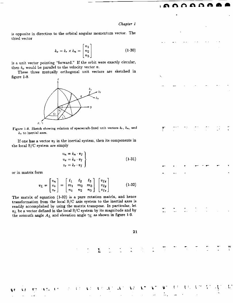
is opposite in direction to the orbital angular momentum vector. Thethird vector
i ]ev =- er × en = n2 (1-30)
n3
is a unit vector pointing "forward." If the orbit were exactly circular,
then _v would be parallel to the velocity vector v.These three mutually orthogonal unit vectors are sketched in
figure 1-8.Z
er
Figure 1-8. Sketch showing relation of spacecraft-fixed unit vectors _r, _n, and_v to inertial axes.
If one has a vector vI in the inertial system, then its components in
the local S/C system are simply
Vn = en " Vl I
Vv = ev " vI
Vr = er "vI
or in matrix form
[vn][,1,2,3]rv, ]v L = Vv = ml m2 m3 |VlyVr nl n2 n3 LVlz
(1-31)
(1-32)
The matrix of equation (1-32) is a pure rotation matrix, and hence
transformation from the local S/C axis system to the inertial axes is
readily accomplished by using the matrix transpose. In particular, let
v L be a vector defined in the local S/C system by its magnitude and bythe azimuth angle A L and elevation angle "/L as shown in figure 1-9.
T
r
A
T"
v -
m.
21
T- "_J
i,

Compilation of Methods in Orbital Mechanics and Solar Geometry
The localvector components are
vn = v L cos "TL sin AL }Vv = v L cos "YL cos A L (1-33)
Vr = VL sin _tL
and the components of this vector in the inertial system are then
VLy[ = g2 m2 n2 Vv (1-34)
VLz J g3 m3 n3 Vr
eT
Figure 1-9. Description of orbiting vector VL in local spacecraft axes definingazimuth A L and elevation angle _/L.
Equation (1-2) then provides the link between the inertial coordi-
nate system and the Earth-fixed coordinate system, and hence, vectorquantities can easily be transformed between the Earth-centered coor-dinate and the local S/C system.
Other instrument or spacecraft-specific coordinate transformations
can, of course, be readily defined relative to the local dynamic coor-
dinate system defined by equations (1-33). One has merely to chainthe sundry transformation matrices together to provide transformation
links between any of them and the inertial or Earth-fixed systems.
Time
The concept of time is one that most of us take pretty much forgranted. But time is one of the most difficult concepts to resolve in
orbital mechanics and astronomy because of the many very small effects
that creep into its measurement and definition. As precision methods22
V_ t ?r
if:- t; t I _'" '' !: L"_ it " . -

ChapSer i
were developed, many time concepts have had to be redefined because
parameters which were once thought to be constants or absolutes werefound to be indeed variables. Entire books have been written on
this subject alone. Consequently, the following discussion will treat
only the main features of time and will serve only to permit the
gross features of and differences between sidereal time (or time with
respect to the fixed stars) and solar time (time with respect to the
Sun) to be understood and appreciated. Chapter 10 of Green (1985)contains a fairly thorough discussion of the various times considered in
modern astronomy. However, these concepts are generally much more
stringent than those required in most Earth orbital applications of orbit
mechanics theory. (See also Smart 1977, chap. VI.)
In figure 1-10 is shown a portion of the Earth's orbit around the
Sun. Suppose that, at point (!), there are two observers on the Earth
located exactly 180 ° apart in longitude. Observer A is watching thestars and observer B is watching the Sun. Suppose further that theyare in constant communication with each other (relativity effects are
ignored) and that at the exact instant that observer A reports a star onhis meridian, observer B reports that the center of the Sun is exactly on
his meridian. Now, observer A has been watching the stars for years.
He has constructed a clock, based on stellar time, which is extremely
(infinitely) accurate. He has defined 24 hr of sidereal time as the intervalbetween two successive passages of the same star over his meridian (see
the note at the end of this chapter). Each hour is divided into 60
sidereal rain and each minute into 60 sidereal sec. Observer A has set
and calibrated an identical clock which he has given to B. So, at the
instant _, both A and B start their clocks.
///Earth orbit
A_ aj
B®
Figure 1-10. Position of Earth relative to Sun on two consecutive days, (_) and
_), and 6 months later, t_).
23
\
\,

Compilation of Methods in Orbital Mechanics and Solar Geometry
At point {_) (fig. 1-10), which occurs one "day" later, observer Acalls out that his star is again on his meridian and that his clock reads
24 hr. Observer B notices that, sure enough, 24 hr has passed on his
clock too, but the Sun has not yet appeared on his meridian. In fact, hefinds that he must wait an additional 3 rain and 56 sec for the Sun to
line up in his instrument. The following day, he finds that he must wait
7 rain 52 sec, etc., with each day being about 3 rain 56 sec longer thanthe day before. At the end of one full revolution of the Earth around
the Sun, 1 yr, observer B finds that his observation of the Sun's centeron the meridian is exactly 24 sidereal hr late.
When the Earth arrives again at point (D, 1 yr later, observer B
would find that he has made 365.2422 revolutions with respect to the
Sun. Observer A, of course, would find that he has made 366.2422
revolutions with respect to the fixed stars. (When B makes one dailyrotation with respect to the Sun, A has made one full revolution with
respect to the stars plus a little more--in fact, 3m56 s more, or a in
figure 1-10. These "little mores" add up to exactly 1 full day in 1 yr.If the Earth were not rotating, the Sun would still make one apparentrevolution around the Earth in 1 yr.
Now, observer B finds that the amount he must wait each day forthe Sun to appear on his meridian is not exactly 3m568 every day. The
interval is somewhat longer in December and shortest in September (seefig. 1-11), but the mean, averaged over 1 year, is 3 rain 56 sec
1440 rain/day= 3m56s.5554
365.2422
Observer B correctly attributes these daily variations to two factors--
the apparent orbit of the Sun around the Earth is not a circle but an
ellipse and the ecliptic, the plane in which the Sun appears to move, isinclined to the equator. Both these factors cause a nonuniform motionof the Sun about the Earth (fig. 1-11).
Figure 1-11 shows a plot of the difference between the solar day and
86400 mean solar sec for each day of the year. The solar day is longestin late December for two reasons: (1) the Earth is near perihelion and
has the largest angular velocity in its orbit and (2) the Sun is also near
the winter solstice, and consequently, is moving essentially parallel to
the equator. The solar day is shortest in mid-September (and almostas short in mid-March) because the Sun is crossing the equator at these
times and hence has the smallest component of its angular velocityprojected onto the equator.
24
r L
L
;" !:

Chapter 1
30
20
10
At, sec 0
-10
-20
-300
LJ
l I [ 1 I I I L40 80 120 160 200 240 280 320 360
Days from January 0L i L L [ L L L [ E [ JF M A M J J A S 0 N D J
Month
J400
Figure 1-11. Plot of quantity At = Length of solar day - 86400, in mean solarseconds, versus day of year.
Observer A now asks the very legitimate question: Why can't B use
A's clock to keep his (B's) time? The answer is, of course, that he can,but B would not find this aesthetically pleasing and it would, in fact,
cause him considerable "headaches" later on. If B used A's clock, then
at the starting position shown at (D in figure 1-10, B would define histime as local noon and A's time as local midnight. A new day would
start for A and would start for B 12 hr later. However, 6 months later,
A and B would be at position _ of figure 1-10. Now, keeping A's time,
midnight for B would occur when the Sun is directly overhead on his
meridian, that is, at midday. Also, during the 6 months which have
elapsed, if B retains the notion to start a new day 12 hr after the Sun isdirectly overhead for him, he would find that the change from one dayto another would occur at various times of day throughout the year.
This would certainly lead to some confusion if not some real practical
difficulties.
Long before the beginnings of recorded history, man has regulated
his everyday affairs by the Sun--working, hunting, etc., by day and
sleeping at night. Since even now, most people work during the day,it is convenient to have days change from one to the other during the
hours of darkness, that is, at midnight. Therefore, a time geared to the
Sun would be extremely useful. However, the direct use of the observed25
2
.-L .....

Compilation of Methods in Orbital Mechanics and Solar Geometry
Sun would produce days which vary in length throughout the year forthe reasons mentioned earlier.
In order to construct a clock which keeps uniform solar time of
some sort, B proposes the use of a fictitious Sun, the fictitious meanSun, which orbits the Earth in the equatorial plane, rather than the
ecliptic, and moves at a uniform rate such that the fictitious mean Sun
completes one revolution about the Earth in exactly the same time
period as does the true Sun--i.e., in 365.2422 mean solar days. Sincethe fictitious Sun moves in the Earth's equatorial plane at a uniform
rate, its right ascension is increasing at a uniform rate. The difference
between the right ascensions of the mean Sun and the true Sun is called
the equation of time (see fig. 1-12):
ET = RAMS - RATS (1-35)
and can readily be computed from simple orbit mechanics (see, forexample, Smart 1977) and, to terms of the second order in the Earth's
eccentricity, is given in units of radians by
ET = y sin 2L- 2ee sin Ms + 4yee sin Ms cos 2L
-_y sin 4L- ee2 sin 2Ms+... (1-36)
where
y = tan 22 (1-37)
E = obliquity of ecliptic, equation (1-21)
ee = eccentricity of Earth orbit
= 0.0167514 - 0.0000418Tu - 0.000000126T_ (1-36)
and where the right ascension of the mean Sun, RAMS, and the Sun's
apparent mean anomaly (see chap. 4 for the definition of some of the
orbital element concepts given here) are given by (Escobal 1968)
L --- RAMS (eq. 1-19) or L + A¢ cos e if correction
needed
M8 = 358°.475644 + 35999°.04975Tu _ 0o.00015Tu2
- 0°.00000333Tu 3
(1-39a)
(1-39b)
26
\
\Ft .
\
"\\

Chapter 1
Z
yMean Sun
:r,-)
Figure 1-12. Sketch showing geometrical relationship between true Sun and meanSun.
The nonlinear terms in this equation are due to the easterly motion
of the Earth's perihelion.
See chapter 10 of Green (1985) for a modern definition of E T and
an equation for its calculation. The concept of the equation of time is
no longer used in modern astronomy, although as a computational tool,it is still quite useful. The fall from grace of this concept came aboutwhen it was discovered that the rotational speed of the Earth about its
axis was not truly a constant. The time definitions we have given are,
therefore, only approximately correct, as they hinge on the constancy of
this quantity. Equation (1-35) is still correct, however, if ephemeris time• P . .
is used. Ephemeris time is the time used in the differential equationsof motion. It is thus based on a dynamical concept, rather than the
geometrical concepts used up to now.When B sets his clock to the fictitious mean Sun, he is now
measuring mean solar time, or more commonly, the ordinary clock time,with which we're all familiar. The international time, universal time,
formerly called Greenwich mean time, is computed as mean solar time,with Greenwich mean noon being the instant that the mean Sun is on
the Greenwich meridian.
As pointed out, many of the simplified time concepts discussed here
are only approximately true because they depend on the constancy ofthe rotational rate of the Earth with respect to the fixed stars. Within
the last half-century or so, it was found that this premise is not strictly
true, and other definitions of time, which do not depend on the Earth's
rotation, have been introduced. These very small differences, however,27
\
N
r " ..... -:
f.

Compilation of Methods in Orbital Mechanics and Solar Geometry
are generally of little importance in applications of these equations toEarth orbit mission design and studies and are generally ignored. These
concepts are quite accurate enough for determining the position of theSun, for example, as will be shown in chapter 5. Most of the new texts
on Spherical Astronomy address this question of time most adequately.(See, for example, Green 1985, Taft 1981, Taft 1985, and the edition of
Smart's classical text revised by Green listed herein as Smart 1977.)
In practice, of course, it would be impractical for every locationon the surface to keep its own mean solar time. To standardize this
somewhat, the Earth was, by international agreement, divided into 24
time zones of approximately 15 ° of longitude. The time zone centered
at 0 ° of longitude, the Greenwich meridian, and extending for 7.5 ° oneither side of the 0 ° meridian keeps Greenwich mean time. The time
zone at 15°+ 7.5 ° west is the first time zone, and so on. For the United
States, eastern standard time is referenced to the 75th meridian, centraltime to 90 °, mountain time to 105 °, and Pacific standard time to 120 °
west longitude. Thus, since 75 ° W corresponds to 5 hr of time we can
convert standard times in the four time zones to GMT as follows:
Eastern standard time + 5 hours }
Central standard time + 6 hours
Mountain standard time + 7 hours = GMT
Pacific standard time + 8 hours
(subtract 1 hour from these numbers for daylight savings time).
With all the perturbations and undulations which time can take, thereally important thing to remember for our purpose is that a sidereal
year has 366.2422 mean sidereal days, and the mean solar year has365.2422 mean solar days. Thus,
366.242224 hours of mean solar time = 24 x365.2422
= 24h3m56s.555 of mean sidereal timeand
24 hours of mean sidereal time = 24 x 365.2422366.2422
= 23h56m48.091 of mean solar time
The ratio 365.2422/366.2422 is, of course, the ratio of any (mean solartime interval)/(mean sidereal time interval). This is the source for
the weird-looking constant 0.25068447 in equation (1-14). The Earthrotates 0.25 ° in 1 sidereal min. Therefore, in 1 mean solar rain it rotates28
T
l

Chapter 1
366.2_t220.25 × - 0.25068447 deg/mean solar rain
365.2422
Note: the scenario between the two astronomers was, of course,
highly simplified in many ways, and in fact, one concept used was
intentionally erroneous at that point for clarity. A sidereal day is
actually defined as the time interval between two successive passages
of the vernal equinox over the same meridian, rather than the intervalbetween two successive passages of a fixed star (one whose proper motion
is essentially zero}. Since, as mentioned earlier, the vernal equinox
is moving westward at nominally 50 arc-sec/yr, the sidereal day is
actually a bit shorter than it would be if the fixed star were used for
time definition. The precessional constant is 50.g564 arc-sec/yr and
is measured along the ecliptic. Its component along the equator is
thus 50.2564 cos e3.44 = 46.1091 arc-sec/yr, or 0.19694 arc-sec/meansidereal day, and hence, the day as defined is 0.12624/15 or 0.008416
sidereal seconds shorter than it would be if it were defined relative to
the "fixed" stars. This amounts to about 1/120 sec. (See, for example,
Motz and Duveen 1966.)
\\
y_- w- -- • -
\•
\
29
r
_k _ iS _-


Chapter 2
Gravitational Field of the Earth
The external field of the Earth can be described mathematically
in many ways. Because of its rotation, and its plasticity, especially
during its early formative years, the Earth is very nearly an oblate
spheroid. Hence, for many analytical purposes, it is convenient to ex-
pand the Earth's external gravity field in a series of spherical harmonics
(Heiskanen and Moritz 1967, p. 59):
V = E Anrn rn+l +n=O m=O
in which t# and A are the latitude and longitude, respectively, and r is
the distance from the origin to the point at which the potential is to be
computed. The constants Anm and Bnm are integrals determined bythe internal mass distribution of the Earth, and
Rnm (¢, A) = Pnm (sin _b) cos mA
Shin(V, A)= Pnm(Sin _) sin mA
(2-2)
(2-3)
in which Pnm are associated Legendre polynomials, are the spherical
harmonics.
The integrals Anm and Bnm are in practice determined from the
precision tracking of large numbers of Earth satellites and then per-
forming statistical fittings to inverted data to determine the values forthese constants, which best fit the observed tracking data. The God-
dard Space Flight Center (GSFC) has done much of this work to high
precision.
Equation (2-1) essentially assumes that the Earth is a distortedsphere. The n = 0 term is the spherical part of the gravity field (the
inverse square part), and the subsequent terms are needed to describe
the departure of the body from sphericity--the greater this departure,the more terms are needed to describe the external potential to a specific
accuracy, and the larger are the constants Anm and Bnm.
PR_CEDI:N_ PAGE BLANK NOT FILMED 31
i
\
A.
r v -
• ., 2 ,

Compilation of Methods in Orbital Mechanics and Solar Geometry
The central force part of the gravity field is usually described by theterm
Vcf = P- (2-4)r
where # is the gravitational constant. If one takes the n = 0 terms out
of equation (2-1) and writes successively
V = A_..._+ E AnmRnm(¢'A) Snrn(¢,A)r rn+l + Bnrn rn+l
n=l m=O
=-_ I+ [Jnmn,_m(¢,A)+KnrnSnm(¢,A)] 2-5)r
n=l m=O
where
AOO = #
Rne dnm _ AnmAO0
RnKnm_ BnmAO0
and Re is the "equatorial radius" of the body, then equation (2-5), as
written, describes the gravity field as a central force term (the term #/r)plus a "perturbation potential" (the summation terms of eq. (2-5)).
If the origin of the coordinate system coincides with the center of
the mass of the central body, a usual assumption, then (Heiskanen andMoritz 1967, p. 63)
J10=Jll =K]I =0
and we write equation (2-5) as
v = _z _+ [J._ R_(¢,_)+K._ S._(¢,_)]r
n=2 m=O(2-6)
The various types of harmonics in equation (2-6) are sketched infigure 2-1 and are identified by
m = O, zonal harmonics
m = n ¢ O, sectorial harmonics
m _ n ¢ O, tesseral harmonics
32
?,-- r
-,2 L

h_g_g_C_nAA
Chapter
Zonal Sectorial Tesseral
P,_o Pnn P,_m
(,_,:_o) (,_# m # o)
Figure 2-1. Sketch showing various types of harmonic coefficients. White areaimplies elevation above; black, elevation below mean spherical surface.
The zonal harmonics are functions of latitude only and hence can only
reflect north-south variations in the gravity field.
Many of the precision orbit prediction programs used by GSFC,NOAA, and others use large numbers of terms from equation (2-6).
GSFC, for example, has (at least) two such programs, one of which goes
up to n = m = 8 and the other to m = n = 21. The GEM-8 model is the
one used for SAGE I and II and SAM orbit work (these programs include
other than gravitational effects, e.g., drag, atmosphere models which are
affected by sunspot activity, relativistic effects, other planetary effects).
For many applications it is generally found that the sectorial and
tesseral harmonic terms in equation (2-6) can be neglected and that onlythe first few zonals are needed. Thus, if we retain only the m = 0 terms,
then all the Knm terms vanish, and letting Jno = .In, equation (2-6)
can be written as
[ ]Y = _ 1 + _ Jn Pn(sin ¢) (2-7)r
n=2
where Pn is the nth-order Legendre polynomial. The first few of these
are (Heiskanen and Moritz 1967, p. 23)
P0(x) = 1Pl(x) = x
1
33
T" ,
\
5

JL" L"I g AAA
Compilation of Methods in Orbital Mechanics and Solar Geometry
and the rest can be generated from the recursion formula
P,(x) - (n- 1) (2n + 1)xPn(x )n Pn-2(x) + -- (2-8)n
If we go as high as J6, we can write equation (2-7) as (Escobal 1965)
r 2- (1-3 sin 2 ¢)+-_- (3-5 sin 2 qJ)
×sin ¢--_ (3-30 sin 2 ¢+35 sin 4 _p)--_
x (15-70 sin 2 g,÷63 sin 4 g,) sin
+_-_ (5-105 sin 2 ¢+315 sin 4 ¢-231 sin 6 ¢)+...
(2-9)The constants in equation (2-9), as obtained from GSFC in March 1986,are
= 398600.64 km3/sec 2
R = 6378.14 km
•12 = +1082.6271E-6
J3 = -2.5358868E-6
J4 = - 1.6246180E-6
J5 = -0.22698599E-6
J6 = +0.54518572E-6
The potential (?q. (2-9)) and these constants are used in some of the
author's orbit programs to generate short-term ephemeris data for use
in the SAGE II and SAM II data reduction. (See chap. 4.)
T
34
i w...... .U £.

Chapter 3
Orbital Elements
As will be seen in chapter 4, the equations of motion in Cartesian
coordinates of a satellite orbiting about an oblate central body (zonal
harmonics only) are rather simple to write, and with modern computers,
it is possible to numerically integrate these rapidly and accurately.
However practical for number generation, Cartesian coordinates arenot the most useful coordinates for visualizing or otherwise describing
a spacecraft orbit. A time sequence of spacecraft position and velocity
vectors by itself has little pictorial value and, consequently, conveyslittle information about the evolution of the orbit.
There are several sets of "orbital elements" used in astronomy,
astrophysics, space sciences, etc., each of which is most useful in
the specialized application for which it was conceived. It takes six
independent coordinates to completely specify the state of an orbiting
spacecraft and permit the determination of its future (or past) state (for
example, three position and three velocity Cartesian components), and
hence, it also takes six independent orbital elements. For Earth orbit
analysis or "Keplermanship" (Escobal's term for playing games with
the two-body equations), the set described below is the one favored by
this writer, in both its utilitarian and interpretive senses.From the first of Kepler's laws, we know that (for central body
motion) the orbit of an Earth satellite is an ellipse with the center ofthe Earth at one of the foci. The ellipse has two axes--the major axis
AB and the minor axis CD in figure 3-1. The origin is at point O, the
center of the Earth. The spacecraft S is located by the radial position
r and the angle f measured from the major axis and where f = 0 is
defined by the radius OA where the spacecraft is closest to the Earth,
the perigee. The equation of this ellipse is
r -- a(1 - e 2) (3-1)l+e cos f
..... .- ° .
v ¸
35
r
t2 t," i_:" i$:_ ( : tL
f,

I&'_I'Zt'a6"_g_AA
Compilation of Methods in Orbital Mechanics and Solar Geometry
a
c
At
Figure 3-1. Geometry of ellipse in plane.
where the two orbital elements,
a = semimajor axis, km
e = eccentricity
determine the size and shape of the ellipse.
For central force motion, the orbit lies in a fixed plane, passingthrough the center of the Earth. Two additional orbital elements
= right ascension of ascending node, deg
i = inclination to equator, deg
locate the position and orientation of this plane in the "inertial"
coordinate system defined earlier. (See fig. 3-2.) Note that by generalagreement, if i < 90 °, the orbit is called a "posigrade" orbit, whereasfor 90 ° < i < 180 °, the orbit is referred to as "retrograde."
The fifth orbital element,
w = argument of perigee, deg
(fig. 3-2), locates the position of the major axis of the orbit in this
plane (more specifically, the position of perigee) and is measured in thedirection of motion from the ascending node of the orbit.
_r _ _ _ _ _ _
r r-.
. v. w
7""
V÷-
36
-± - -- - 2 L.
-t' _t: t_' i" -re7. _7- t' t' _.'" '''_ , _t "_
t ¢"

bg'Id' t' tPlg naA
Chapter S
Z
ojection of orbit onto Earth
Figure 3-2. Sketch defining location of orbital plane and perigee point in inertial
coordinate system.
The sixth element must somehow relate the position of the space-
craft in its orbit to some specific time. The angle f, called the true
anomaly, is awkward to use for this purpose. According to the second
of Kepler's laws, the radius vector of the spacecraft sweeps out equal
areas in equal time increments. Since the spacecraft is closer to the
Earth at perigee (f = 0) than it is at apogee (f = 180), the spacecraft
must move faster at perigee than it does at apogee. This means that the
angular rate df/dt is not constant around the orbit. A mean angularrate of the spacecraft can be shown to be
n = Pe-_-md(3-2)
and is a constant of the orbit for a central force. Let to be the time the
spacecraft last passed through perigee. Then the angle
M = n(t - to) (3-3)
is an angle which has the desirable property of increasing at a uniform
rate. This angle is called the mean anomaly and is selected here as
the sixth orbital element. In order to relate the mean anomaly to the
true anomaly, we must first introduce a third anomaly, the eccentric
anomaly E, which relates f to M as follows:
37
t

i tt'itt"at t'ttAAih
Compilation of Methods in Orbital Mechanics and Solar Geometry
E 1 - e f (3-4)tan_-= _lll---_e tan
and Kepler's equation
M=E-e sin E (3-5)
These transcendental equations are still not directly solvable (i.e., to
find f given t). However, for orbits with small eccentricity (near-circular
orbits) as most near-Earth orbits are, the following series (Smart 1977)is useful--angles are in radians:
(E=M+ e- sin M+-_- sin 2M
3e 3
+ _ sin 3M+... (3-6)
f=M+ 2e- sin M+T sin 2M
13e 3
+ _-_ sin 3M+... (3-7)
If the eccentricity is large, or if extreme accuracy is needed, the Taylorexpansion of equation (3-5) gives the iteration formula
En+ l + En -= MT- Mn1- e cos En
in which, given the true value of MT, find En from equation (3-6) andMn from equation (3-5). Then equation (3-8) gives a corrected value
En+]. For a second iteration, set En = En+] from the last iteration,
and repeat to convergence. This procedure generally converges to sixor seven decimals in three or four iterations, even for values of e nearunity.
There are two basic advantages for using orbital elements. First, theorbit is much easier to visualize, as the orbital elements describe the
total geometry of the orbit--its size, shape, and orientation in space.
Second, and perhaps more important, if the Earth were a perfect sphere
(i.e., the gravity field describable by the inverse square law only) and
there were no other external forces acting on the spacecraft, then five of
the six orbital elements--a, e, i, _, and _--would be constants, only
M would change with time, and this change would be a simple linear
one. Even for a spherical Earth, all six of the Cartesian Components
change continually and dramatically with time at each integration step.38
Ir
r _ _ _ t ,_.
rt;

Chapter 3
It seems reasonable to expect, then, that if the gravitational poten-
tial field of the central body only deviates very slightly from that of a
sphere as does the Earth, the orbital elements a, e, i, 12, and _; wouldchange very slowly with time, if at all, and these changes would be
predictable to varying orders analytically. This is, of course, preciselywhat happens for an Earth satellite. Very detailed and complex analyt-
ical studies (e.g., Kozai 1959, Brouwer 1959, King-Hele 1958, Garfinkel
1959, Merson 1961) show that it is possible to account for practically all
the oblateness perturbative effects of the Earth with a single term (./2),and to first order it is found that a, e, and i are constants, and f/and w
change linearly and slowly with time (order of a few degrees per day, or
less, depending on the inclination of the orbit). These changes are easy
to compute (Escobal 1965 or McCuskey 1963). After the equations ofmotion are introduced in chapter 4, a brief series of numerical exam-
ples will show the effects of various harmonics on both the Cartesian
components and on the orbital elements.It is, of course, possible, if not imperative, that we be able to transfer
from Cartesian coordinates to orbital elements and vice versa. The
following algorithms, applicable to circular and/or elliptical orbits only,are used for this purpose (see, e.g., Escobal 1965 or McCuskey 1963).
1. Orbital elements to Cartesian coordinates (CONCAR)
(a) Find E from (M, e) as described earlier (eq. (3-6))
(b) Then
= a(cos E - e)
Z_ = a V/1 - - e2 sin E
5:_ =-a/_ sin E
_ = a/_ vq - e2 cos E
where
1- e cos E
(c) Compute the unit vectors
[cos w cos 12-sin w sin 12 cos ll/b = /cos ¢z sin f/+ sin _z cos f_ cos
L ]sin _ sin z
-sin w cos f]- cos w sin f_ cos i]J-sin w sin fIcos+ coswsln'Wcosz. f_ cos39
i_ a
\
P
_1 t_;. It-.
t, t.' t ' 1,." t '" _1, ' _1,"

40
Compilation of Methods in Orbital Mechanics and Solar Geometry
(d) Then compute the spacecraft position and velocity vectorsfrom
r = x_/b + ywQ
2. Cartesian coordinates to orbital elements (CARCON)(a) From angular momentum vector
h=rx÷= zx z_ = i cos f/
zy yz cos i
Find h, i, and f_
(b) With r = Irl, v = Ivl, find the semimajor axis a from
1 2 v 2
a r D
where for the Earth, p = 398600.64 km3/sec 2.
(c) Find the eccentricity
e=v_ h2#a
(d) Define u = w + f, then
r cos u=x cos f/+y sin f/z
r sin u-sin i
which gives the proper quadrant for u
(e) Find the true anomaly f
e cos f = p -1r
e sin f =_
where p = a(1 - e 2)
(f) Finally, then,
(g) Find E from equation (3-4) and M from equation (3-5).
lr - r-.v'-

it, lilfft £'i g!l ml A
Chapter 3
This completes the orbital element set.
Note that these equations even hold for circular orbits (e = 0), if we
agree to set w = 0 and measure f (or M, E) from the ascending node
of the orbit.
The algorithm, CONCAR, changing from orbital elements to Carte-sian coordinates, is quite useful in determining time histories of the
Cartesian coordinates, which parameters are frequently used in deter-
mining other geometric parameters and properties in which the mission
design engineers might be interested. Given the set of orbital elementsat time to, the mean anomaly M is found at t + At from equation (3-3)
as
M= Mo+n At
The eccentric anomaly is found from equation (3-6), as described earlier,and then the Cartesian state vector is found from the algorithmic
equations. This process can be repeated at any time interval At, andthe results hold as long as only a central force field (all ,In = 0) can be
assumed. In actual practice, this time might be of the order of 10 rain
or so, and then the small perturbations begin to make themselves felt,
and another algorithm, to be described in chapter 4, must be used.
This requires using the analytical expressions for _b and _ explained in
chapter 4 to continuously update w and 12, thus enabling the algorithmCONCAR to be used over extended time periods.
A third algorithm, especially useful if one wants to preserve the
identity of the initial Cartesian coordinates, is the so-called f- and
g-series method. (See, for example, Escobal 1965.) Here, the radius
vector r(t) and vel¢_city vector _(t) at any time t are expressed in termsof the initial values of the position and velocity vectors, and the f(t, to)
and g(t, to) parameters
i'(t) = f(t, to) ro + g(t, to)i'o (3-8)
= f(t, to) ro + to)to (3-9)
where ro and ro are the initial position and velocity vectors, respectively.
The f and g terms were originally derived as an infinite series involving
the zeroth, first, and second derivatives of the position vector asconstant coefficients and the time as the independent variable. However,
for central force motion, these series can be expressed in analytical form
1t8
f(t, to) = 1 - a [1 - cos (E - Eo)] (3-10)ro
41
r - r r
r 11" _ ,r _ _.
/d
°_
il: t: t t'" '',

g tifft gtrl
Compilation of Method8 in Orbital Mechanics and Solar Geometry
g(t, to) = t - [(E - Eo) - sin (E - Eo)] (3-11)
and
f(t, to) = -t _/-_-_asin (E- Eo)V fro
g(t, to) = 1 - a [1 - cos (E- Eo)]r
(3-12)
(3-13)
in which
r = a(1 - e cos E) (3-14)
The parameters a, e, and Eo are computed from algorithm 2
(CARCON) at t = 0, and E at any subsequent (or previous) timecan be found from equation (3-6) with the help of the iteration process
described previously. This procedure offers no real computational ad-
vantage over that of algorithm 2 alone. It has, in fact, the disadvantageof not readily incorporating the oblateness effects through the _ and _b
terms as described earlier. It does, however, retain the identity of the
initial Cartesian state, as mentioned, and is quite useful in studyingthe effects of errors in the initial conditions, as the variance-covariance
matrix of errors in the values of future coordinates can be constructeddirectly from equations (3-8) and (3-9).
As pointed out earlier, five of the six orbital elements would be
constant if the Earth were a perfect sphere and there were no other
outside perturbations acting on the orbit. The effects of the nonspher-
ical components (in the spherical harmonic sense) of the gravity field,
the perturbation forces, are very small for a typical Earth satellite, and
hence, the orbital elements, instead of being constant, vary very slowly
in time. The most elaborate analyses referenced earlier (Kozai 1959and the others) indicate that these changes are combinations of thefollowing:
Secular changes: these are linear, or at best quadratic, changes, which
always proceed in the same direction. The elements _, w, and Mare the only ones which experience secular changes.
Long-period terms: periodic changes of small amplitude whose periodsare of the order of 80-100 days and longer.
Short-period terms: periodic changes of small amplitude whose periods
are small (integer or half-integer) multiples of the orbital period.
These terms are sketched in figure 3-3.42

Chapter3
Escobal (1965, chap. 10) discusses perturbations of the orbitalelements thoroughly, as does the classical text by Moulton (1914). A
typical orbital element can be most generally represented by an equation
of the form
q=qo+it(t-to)+K1 cos 2_+K2 sin (2f+2w)+H.O.T.
where
= secular term
qo = mean value of the element
K1 = long-period term
K2 = short-period term
Higher order terms (H.O.T.) in other multiples of w and f are, of course,
also present, and any of the constants can be zero.
In any event, as a result of these perturbations, the orbit of an
Earth satellite is never a true ellipse. However, as seen in the preceding
algorithms, the specification of the spacecraft state vector permits the
computation of a unique set of orbital elements, and thus at each instant
of time, a unique set of orbital elements can be associated with the orbit.
If at a given instant of time all the gravity perturbations were turned
off and only the central force part of the gravity field were allowed to
remain, the spacecraft would then truly be in the elliptical orbit defined
by the orbital elements at that moment. This constantly changing setof orbital elements is referred to as the set of osculating elements and is
specified at a unique time. Point a at time t in figure 3-3 identifies the
osculating element at this time. It has been found through many sets
of calculations that, if one determines the set of osculating elements at
one time, say T, and then uses that set as described above to advance
the position of the spacecraft along the orbit, then considerable error
in the predicted Cartesian state may develop quite rapidly. The reasonfor this is that there may be considerable deviation in the value of a
given element in different points of the orbit. (Compare points a and
b in fig. 3-3.) For example, in a spacecraft orbit of small eccentricityat an altitude of 600 km and inclination of 57 °, the mean value of the
semimajor axis is 6981 kin. However, the actual value can range from aminimum value of about 6976 km to a maximum of 6986 km. Table 3-1
shows the differences in mean anomaly that one would compute at
various time intervals using these values of a.
43
r v- _ r
v-
k: -Z LL
' t'- " !: t."

Compilation of Methods in Orbital Mechanics and Solar Geometry
Element
t=0
Unperturbed
Time
Figure 3-3. Sketch illustrating various orders of perturbations.
Table 3-1. Change in Mean Anomaly for +5-km
Change in Semimajor Axis
a, km n, deg/min Mat t = 100min, deg
6976 / 3.725059 372.50596981 3.721058 372.1058
6986 3.717064 371.7064
Since 1 ° represents a down track distance of about 122 km for this
orbit, table 3-1 represents a potential difference of about 97 km in only100 rain, which is about 1 revolution for this orbit. Even if the first-
order perturbations are included as described in chapter 4, rather largeerrors still ensue after only a short time.
Experience has shown that much greater accuracy is maintained
over long time periods if the mean elements are used. Perhaps a betterway of saying this is to say that a more acceptable error results which
allows the simple algorithm to be used over a longer period of time.Relations for the osculating elements in terms of the mean elements
can be found in the references by Kozai (1959), Brouwer (1959), et al.
cited earlier. These same relations can be used iteratively to computethe mean elements from the osculating set at any time.
v_
v - ,m
44
L

h L,,_ tt_ tt'l t_ g_ A A A
Chapter 4
Equations of Motion
The development of the general equations of motion for a satellite
of negligible mass orbiting about a massive primary, or central body,can be found in practically any textbook on Celestial Mechanics. (See,
for example, Escobal 1965, Smart 1977, Dubyago 1961, or the classical
text by Moulton (1914).) In vector form
d2r
dt 2 =vV (4-1)
where r is the radius vector from the center of the primary (the origin of
coordinates for this development) to the spacecraft, t is time, and V is
the gravitational potential of the central body. If we restrict ourselves
to the 6th-degree zonal expansion of equation (2-9) and recall that
Z
sin _-r
then we can write the three components of equation (4-1) as (see, for
example, Escobal 1965)
d2z c3V
dt 2 Ox
px 3 2
5j z 2
'
} (4-2)
45
\
\
t_
"3,w-
1. r "
f.
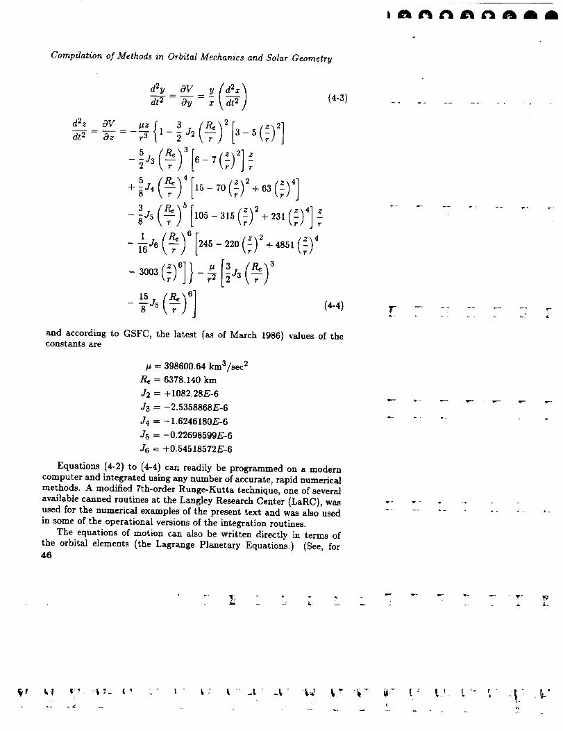
Compilation of Methods in Orbital Mechanics and Solar Geometry
d2y OV _ {a_
dt 2 - Oz -- -_ 1-_J2 3-5
2J3 6-7 -9-
,]-_ 5 105 315(z) 2 4 r- +231(z)
-_ 6 245-220(z)2+4851(z) 4
(4-3)
(4-4)
and according to GSFC, the latest (as of March 1986) values of theconstants are
# = 398600.64 km3/sec 2
Re= 6378.140 km
J2 = +1082.28E-6
J3 = -2.5358868E-6
•14 = -1.6246180E-6
•15 = -0.22698599E-6
J6 = +0.54518572E-6
Equations (4-2) to (4-4) can readily be programmed on a modern
computer and integrated using any number of accurate, rapid numericalmethods. A modified 7th-order Runge-Kutta technique, one of several
available canned routines at the Langley Research Center (LaRC), wasused for the numerical examples of the present text and was also used
in some of the operational versions of the integration routines.
The equations of motion can also be written directly in terms of
the orbital elements (the Lagrange Planetary Equations.) (See, for46
!r
It-
v - y
T
L

Chapter
example, Escobal 1965, Smart 1977, Dubyago 1961, Moulton 1914.)
The perturbative gravity field, however, becomes very messy when
expressed in terms of the orbital elements. Consequently, this form
of the equations of motion, while occasionally used in numerical work,
is mainly used in theoretical developments, in which usually only the
J2 or the J3 term of the zonal expansion is used in an attempt toderive purely analytical expressions for the response of the spacecraft
orbit to these terms. (See, for example, Kozai 1959, Brouwer 1959,
Garfinkel 1959, King-Hele 1958.) Escobal (1965) expounds somewhaton Kozai's method and gives a lucid physical explanation of the effects
of the perturbations on the orbital elements. (To this end, see also the
excellent presentation by Moulton (1914).)
As mentioned earlier, the perturbing potential is difficult to expressin terms of the orbital elements and, with modern computers and
numerical techniques, it is the author's contention that, if one is merely
seeking accurate numbers with which to work, then the integration of
equations (4-2) to (4-4), or in their more complete form equation (2-6)
for the potential, is as good a way as any. Of course, if one is faced
with the problem of predicting the position or orbital characteristics
far in the future--for example, for several weeks or months---obviously
integration of the equations of motion would become quite expensive. In
this case, one would probably be well advised to sacrifice some accuracy
for economy and speed and use one of the theoretical models alluded to
earlier or the simple mean element model shown later in this chapter
which uses only the ,/2 term.The first numerical examples are shown to illustrate the accuracy
of equations (4-2) to (4-4). An initial state vector
z = 3211.365 km
y = -4680.423 km
z = -4081.154 km
= 2.326315 km/sec
_/= 5.555629 km/sec
,_ = -4.545389 km/sec
was picked from an ephemeris tape prepared by GSFC for the SAGE II
experiment. The GSFC prediction program, as mentioned earlier, usesan n = m = 8 gravity field (eq. (2-6)) and serves as a standard here
with which other computations are compared.
w_
47
_._ _ _ -_ __

fft n N A A A
Compilation of Methods in Orbital Mechanics and Solar Geometry
The same initial conditions were used in the integration of equa-
tions (4-2) to (4-4) with three runs:
1. All J2-J6 used
2. J2-_ 0, J3-J6=O
3. All J2-J6 = 0
Run 3, of course, corresponds to the purely central force field. The
results of these runs are given in table 4-1 as follows: the first column
lists the GSFC results after 48 hr (2880 min), 96 hr (5760 rain), and
144 hr (8640 rain). Columns 2-4 list the differences
(LaRC results of runs) - (GSFC results)
and the LaRC results were computed from the modified Runge-Kutta
numerical method with a 60-sec time increment for the computationinterval.
Table 4-1. Comparison Between GSFC and LaRC Ephemerides
Run 1 includes all J2-J6; Run 2 uses J2 only; ]Run 3 is spherical Earth result J
48
x, km . . .
y, km . . .
z, km . . .
_, km/sec
y, km/sec
,_, krn/sec
GSFC
-2414.451
-5520.263
3521.274
3.1777850
-4.6332890
-5.0583560
Differences in LaRC mad GSFC resultsfor--
Run 1 Run 2 Run 3
t = 48 hr
-3.087
4.505
4.912
-0.002647
-0.006146
0.003965
-3.686
5.144
4.763
-0.002981
-0.006592
-0.003546
t---- 96 hr
591.649
-57.877
257.880
0.504577
O.140997
0.223293
*, km . .
y, km .
z, krn . .
_, km/sec
y, km/sec
_, km/sec
-2767.378
3806.603
5141.751
-2.997119
-6.258721
3.014856
4.915
10.928
-4.985
-0.005224
0.007867
0.010240
t = 144 br
5.892
12.370
-4.834
-0.006453
0.008922
0.009824
-788.005
-212.267
-341.438
1.376789
-0.183703
0.608086
Z_ knl . .
y, km . .
z, km . .
x, km/sec
_), km/sec
_, km/sec
3164.478
5901.433
-1980.466
-2.952138
3.573608
5.968511
6.164
-7.421
-13.117
0.008289
0.015006
-0.005320
7.876
-6.162
-11.255
0.009102
0.013410
-0.005758
-2011.458
354.769
-694.553
-1.038673
-0.310911
-0.443209
r ._.
_- - v.-- w,-- v - ,
v
k

Chapter
It is seen from table 4-1 that the use of only the J2-J6 terms of the
gravity field expansion is not too shabby when compared with the full-
blown 8 by 8 model of GSFC and is certainly accurate enough for many
satellite applications. Equally obvious from the table is the fact thatthis model is probably not accurate for other applications--for example,
long-range prediction (i.e., several months) of the ground or geodetic
position of the spacecraft to be used for ground truth location studies.
However, even for 6 days of integration, the differences between thestandard GSFC model and the truncated model used herein are only
of the order of 10 km or so in position and of the order of 15 m/sec in
velocity.
The J2 term clearly dominates the perturbation effect, a fact whichhas been known since the early days of satellite flight. In fact,
examination of the table shows that, at least over the 6-day period
used for the example, the use of the J3-J6 coefficients is not warranted
at all. However, only further study could determine the time span in
which their exclusion should be adopted; for example, their effect would
doubtless show up for an integration span of several weeks.
If one now converts the Cartesian components of table 4-1 to
orbital elements using the CARCON algorithm, one finds the results
of table 4-2. Here, the complete values are presented, not merely thedifferences between the LaRC and the GSFC results. The actual orbital
elements at t = 0 hr were
a = 6981.471516
e = 0.00141817
i = 570.002219
= 96o.623064
w = 58°.316978
M= 165°.753617
km
First, note the last column of table 4-2, which shows the unper-
turbed elements. The agreement of these elements (except, of course,
M) with the initial conditions illustrates the accuracy and stability ofthe numerical integration routine and serves to rule out integration er-rors as a cause of some of the differences in the Cartesian coordinates
of table 4-1.
Second, the orbital elements appear to be very close in all cases.
The percent differences in all elements except w and the anomalies are
very small (order of 0.001 percent) compared with the percent errorin the Cartesian coordinates (order of 0.2 percent). The maximum
errors are in w and f individually. However, and much more important,
4g
r w y
L_
v--
L ¸ /_

Compilation of Methods in Orbital Mechanics and Solar Geometry
the errors in the sum w + f are rather small, and it is the sum
which determines the angular distance of the spacecraft from the
ascending node. The error in w is mainly due to the small eccentricity
of this orbit. As the CARCON algorithm of chapter 3 shows, the
computation of u = w + f does not explicitly involve the eccentricity,but the computation of f does. Therefore, u ought to be determined
with reasonable accuracy, even for small eccentricities. However, when
the eccentricity is small in absolute value, even very small absolute
errors are very large relatively, or percentagewise, and hence the
accuracy to which f, and consequently w, are individually computed is
questionable. If these are used to determine the Cartesian coordinates,though, the results are still reasonable, as u is the quantity which isused, and this is determined with some confidence.
If one considers only the J2 part of the perturbed gravity field and
further restricts oneself to first-order theory, then one finds that a, e,and i are constants in time for a given orbit. The longitude of the
ascending node, l_, and the argument of perigee, w, are found to varylinearly and are given by the following equations:
= no + - to)w = Wo+ - to)
M = Mo + fi(t- to)
(4-s)(4-6)(4-7)
where
( p_)2fi i (4-8)¢z= cos
_b=_J2 2-_ sin 2 i fi (4-9)
fi----_-3 1+ 5 2(p_-_)_ _sm i (4-10)
and in which
p = a(1 - e2) (4-11)
If equations (4-5) and (4-6) are used to compute I2 and w and equa-tions (4-7) and (4-10) are used to compute M, it is found that the
element-to-Cartesian coordinate algorithm given earlier will predict the
Cartesian components reasonably accurately for longer periods of time
than can be computed from the central force alone (order of a few50
A
v-
4
/
(,

Chapter 4
days), but of Course the acceptable time period depends heavily on theintended use and accuracy requirements.
Table 4-2. Comparison Between GSFC and LaRC Osculating
Orbital Elements Computed at 48, 96, and 144 hr
Run 1 includes all J2-J6; Run 2 uses J2 only; ]Run 3 is spherical Earth result J
LaRC results for--
GSFC Run 1 Run 2 Run 3
t = 48 hr
a t km .....
e .......
i, deg .....
l-l, deg ....
w, deg ....
M, deg ....
f, deg ....
w+ f, deg . . .
6983.088680
0.00186271
6983.070167 6983.090200
0.00184027 0.00181924
6981.471471
0.00141816
57.006807
88.674902
72.635991
70.179204
70.380168
57.006451
88.675025
72.802224
69.955204
70.153465
57.006509
88.667845
74.944251
67.817778
68.010984
57.002221
96.623060
58.318410
81.313131
81.473819
a, km .....
e .......
i, deg .....
i2, deg ....
w, deg ....
M, deg ....
f, deg ....
w+f, deg . . .
143.016159
6977.549839
0.00116235
56.992038
80.804759
89.510732
332.149893
332.087589
61.598321
142.955684
t =96hr
6977.616167
0.00113651
56.991955
80.806862
91.289731
330.265486
330.200812
61.490543
t = 144 hr
142.955235
6977.629441
0.001140987
56.991988
80.792607
98.225995
323.337990
323.259833
61.485828
139.992229
6981.472607
0.00141831
57.002216
96.623066
58.319535
356.872952
356.864070
55.183605
(7- I km .....
i, deg .....
fl, deg ....
w, deg ....
M, deg ....
f, deg ....
w+f, deg . . •
6986.459458
0.00146659
57.014001
72.866127
50.919996
289.476609
289.318070
340.238066
6986.385047
0.00140939
57.015303
72.869378
52.026907
288.229329
288.075816
340.102753
6986.376400
0.00127645
57.015294
72.847804
58.879086
281.390348
281.246913
340.125999
6981.471158
0.00141834
57.002222
96.623062
58.318779
272.434666
272.272271
330.591050
Equations (4-5) to (4-10) were used to generate the next set of
numerical data, again for t = 48, 96, and 144 hr. The set of orbital
elements given above was assumed at t -- 0. The orbital elements
were updated as prescribed, and the CONCAR algorithm was used
to generate the Cartesian components from the orbital elements. Theresults are shown in table 4-3. The first two thirds of the table give the
51
,r r_ r
_.._ --- _.. J t. .... L
'W""
k
f-

hL' t'tg'Zd tg AAA
Compilation of Methods in Orbital Mechanics and Solar Geometry
results of the appropriate calculations, the top third giving the orbitalelements and the middle third giving the Cartesian coordinates. The
bottom third gives the difference in the Cartesian coordinates between
the above results and the reference GSFC results from column 1 of
table 4-1. The bottom third also displays the difference between the
sum w + f computed from the exact Cartesian coordinates and thatcomputed from the approximate orbital elements.
The differences shown in table 4-3 are about an order of magnitudegreater than those found using only J2 with the integration routine.(The integration of the equation of motion includes all orders of effect
and not just the first-order effects predicted by equations (4-5) to (4-7), with a, e, and i constant.) Comparison between tables 4-2 and 4-3
shows that the nodal point _ is predicted rather well by equation (4-5),
and the quantity w + f is the prime error source. However, we
must remember that the approximate orbital element treatment usingequations (4-5) to (4-10) is expressly to be used with mean orbital
elements, while we are here applying these equations to osculatingelements. There may be some instances where we have no choice as
the only initial conditions available may be in Cartesian form, and
these almost always refer to osculating elements. Proceeding with this
caveat, note that the two orbital planes line up rather well but the
position of the spacecraft in the true orbit is slightly ahead of theposition in the approximate orbit. This is, in turn, traced to the fact
that the first-order theory assumes that a is a constant. However, for
this orbit, a varies between 6975.2 and 6987.6 kin, and hence, the timing
between the true and approximate (through the mean anomaly) orbit
is off somewhat and, as can be seen in the last column of table 4-3,
the true spacecraft position is gaining on the approximate position byabout 0.25 deg/day.
The approximate first-order analysis can thus also be reasonablyaccurate for a few days or so. If one starts off with a set of mean
elements, then the spatial position can be predicted reasonably well for
periods of several weeks to several months, depending on the accuracyconstraints imposed on the desired results. This algorithm is rather
simple to program and compute when compared with the integrationroutine described earlier.
Table 4-4 demonstrates the application of this modified algorithm.The mean elements at t = 0 were computed using the method of
Kozai (1959). (These equations are rather lengthy and hence are not
reproduced here. The original reference should be consulted.) The
mean elements a, e, and i were then held constant, and the remaining52
r
T _-
L

Chapter 4
three mean elements updated using the following rates computed from
equations (4-5) to (4-11):
= 223.234095 deg/hr
i_ = -0.16475043 deg/hr
= 0.073098627 deg/hr
Table 4-3. Orbital Elements, Cartesian Coordinates, and Errors in
Cartesian Coordinates Computed With CONCAR Algorithm Using
J2 Term and Starting Conditions as Osculating Elements at t -- 0
e .........
i, deg .......
l-l, deg ......
w, deg ......
M, deg ......
+ jr, deg .....
Z_ km .......
y, km .......
Z_ km .......
5, km/sec .....
y, km/sec .....
_., km/sec .....
Ax, km ......
Ay, km ......
Az, km ......
A_, km/sec ....
Ay, km/sec ....
A_, km/sec ....
A(w-t- f), deg . . .
t=48hr t =96hr t = 144hr
6981.471516
0.00141817
57.002219
88.712177
61.826844
80.515297
142.502536
-2437.812650
-5484.269655
3563.455210
3.157658
-4.681182
-5.023572
23.362
-35.993
-42.181
0.020127
0.047892
-0.034784
-0.513623
6981.471516
0.00141817
57.002219
80.801189
65.336711
355.276977
60.60O278
-2718.177361
3907.133828
5094.024327
-3.050433
-6.184601
3.114084
-49.201
-100.201
-47.717
0.053314
-0.074120
-0.099828
-0.998043
6981.471516
0.00141817
57.002219
72.890102
68.846577
170.038657
338.722663
3232.649280
5811.739703
-2124.784121
-2.863125
3.739829
5.908481
--68.171
89.693
144.318
-0.89013
-0.166221
0.600030
-1.515403
The top third of table 4-4 gives the mean elements at t = 0, 48, 96, and144 hr. The middle third of the table gives the Cartesian coordinates
computed from the CONCAR algorithm and using the mean elements,
and the bottom third gives the differences between the LaRC and theGSFC results as was done in tables 4-1 and 4-3. It can be seen that
these differences in table 4-4, using the mean elements at t = 0, are not
substantially different from those of runs 1 and 2 of table 4-1, beingwithin a factor of 2 or 3 of the integrated results, and certainly much
better than the 1 to 2 orders of magnitude differences displayed in
table 4-3 in which the oscillating elements were used at t -- 0. It53
V
r
_' &
L
.... J ....

Compilation of Methods in Orbital Mechanics and Solar Geometry
can perhaps be implied that the perturbation-modified algorithm using
mean elements can be used, with only a slight degradation in accuracy,
over approximately the same span as the numerical integration using
only the zonal harmonics. It may just be a personal prejudice, butthe author believes that the numerical integration algorithm is more
defensible than the modified mean-element approach, especially if theintegration time exceeds a few weeks. However, the mean-deviant
algorithm has been successfully applied to the prediction of both
SAGE II and SAM II ground truth sites with lead times of as muchas 4-6 weeks.
Table 4-4. Orbital Elements, Cartesian Coordinates, mad Errors in
Cartesian Coordinates Computed With CONCAR Algorithm Using
J2 Term and Starting Conditions as Mean Elements at t = 0
£I I km .......
'e .........
i, deg .......
l'l, deg ......
w, deg ......
M, deg ......
Z I km .......
y, km .......
z, km .......
x, km/sec .....
l_, km/sec .....
_, km/sec .....
AX, km ......
Ay, km ......
Az, km ......
A_:, km/sec ....
A j, km/sec ....
A,_, km/sec ....
t =0hr t--48hr t=96hr t = 144hr
6981.26555
0.00254626
56.997801
96.601960
71.220024
152.821231
2215.11242
-4679.87474
-4089.14043
2.32563390
5.55145098
-4.53986239
3.747
0.548
-7.986
-0.0006811
-0.004178
0.0055266
6981.26555
0.00254256
56.997801
88.693939
74.728758
68.057791
-2409.67576
-5520.91264
3515.54137
3.18182136
!-4.63367603
-5.06051117
4.775
0.133
-5.733
0.0040364
-0.003870
-0.0021552
6981.26555
0.00254626
56.997801
80.785919
78.237492
343.294351
-2755.911096
3819.199893
5130.239109
-3.00963556
--6.25485145
3.03212667
11.467
12.597
-11.512
-0.0125166
0.0038695
0.0172707
6981.26555
0.00254626
56.997801
72.877898
81.746226
258.530911
3176.32012
5889.11718
-2004.32760
-2.94169646
2.59164655
5.95682454
11.842
-12.316
-23.868
0.0104415
0.0180386
-0.0116862
54
_t t2 t* it:- [" t'_• • t
| 1o r "
i
5",

Chapter 5
Where Is the Sun?
Most of the time series relations needed to determine the position
of the Sun have already been given in chapter 1. The remaining
geometrical concepts will be developed in this chapter, as needed.
Perhaps the best way to introduce this material is through numerical
examples. The following problems, typical of those encountered in
spherical astronomical applications, will be addressed in this chapter,and a complete numerical example will be worked out for each to
illustrate the method. The text procedures are not the only approach,
of course, but are the ones that, for now unknown reasons, appealedto the writer at the time he first encountered these problems. The
number of significant figures shown in the numerical results is generally
that required for the accuracy given; 0.1 arc-sec is 0°.000028, andcalculations to a few hundredths of an arc-sec are frequently required.
The most fundamental problem which arises concerning any compu-
tation of the Sun's position is the determination of the right ascensionand declination of the center of the Sun, given any date of the year and
time of day. These coordinates, along with the Greenwich sidereal time,are central to the solution of all the problems listed below. Therefore,
the problems to be considered in the present chapter are the following
(all the problems presented require the day of the year and/or the time
of day to be given; some also require the specification of a particularlocation of the Earth's surface--the coordinates of an "observer;" these
are assumed given):
1. Given any calendar date in the year and time of day, what
are the right ascension and declination of the Sun? Note: Onlymean values will be determined as the extra computation will
serve no useful purpose here.
2. What is the Greenwich sidereal time for a given universal time,
and what is the local sidereal time at a specified geographic
location?
3. What are the geographic coordinates of the subsolar point at a
given time of day?
55
3"- , ,
tr, r_ r - _ r w-
t _ _'" ,-, :!: _"

iC'tf'tC Ctgt tmA
Compilation of Methods in Orbital Mechanics and Solar Geometry
4. For a given observer, what are the azimuth and elevation
angles of the Sun at a given local (zone) time of day (with andwithout refraction)?
5. What is the local zone time when the Sun is directly on thelocal meridian (zonal time of local noon)?
6. What is the elevation angle of the Sun at local noon?
7. What are the local zone times of sunrise and sunset?
8. What are the azimuth angles of the Sun at sunrise andsunset?
Note that if the Cartesian coordinates of a spacecraft are known in
the inertial coordinate system, then its right ascension and declination
can be found from equation (1-1a). Then problems 2-8 can be appliedto satellite motion by substituting the satellite coordinates for those
of the Sun, taking into account, when necessary, the much more rapidtime changes of these coordinates.
As a specific application of some of the concepts discussed here---
given the semimajor axis and eccentricity of a satellite orbit, what mustbe the location of the line of nodes of a Sun-synchronous orbit which
crosses the equator at a specific local time? (See, e.g., Brooks 1977.)
The numerical example will be worked out for the time of April 6,1985, at 2:37 PM EST in Hampton, Virginia, whose latitude andlongitude, respectively, are approximately 37°N and 76°W.
The chapter will terminate with the solution of a problem arising
in connection with Sun-viewing satellites (e.g., SAM, SAGE) andspecifically the problem of reducing the data from these satellites--
namely, what is the minimum altitude of a ray from the center of the
Sun (or indeed any other specific celestial location) to the spacecraftabove the oblate Earth, and what are the geographic coordinates of the
"subtangent" point on the surface of the Earth? (See Brooks 1980.)
Problems and Examples
Problem 1:
Figure 5-1(a) shows the inertial coordinates defined earlier in chap-ter 1. The coordinates of the Sun are the right ascension a and decli-
nation 6. Figure 5-1(b) shows the spherical triangle "),SQ.
For the given date, find the Julian date as outlined in chapter 1.Then proceed by the following steps:
(a) Compute the mean longitude of the Sun, L = M + &, fromequation (1-19)
56
r
kJ,..

Chapter 5
Z
c ipticyx, "3
(a) Sun in inertial coordinate system and its relation to Greenwich meridian.
(b) Blowup of spherical triangle _SQ of figure 5-1(a).
Figure 5-1. Location of Sun in both inertial and Earth-fixed coordinate systems.p
(b) Find the mean anomaly of the Sun, M, from equation (1-39)
and the eccentricity of the solar orbit from equation (1-38)
(c) Compute the quantity f - M from equation (3-7) and convert
to degrees
(d) Then, (_5 + f) = (_ + M) + (f - M)
(e) Compute the obliquity of the ecliptic, e, from equation (1-21)
Then from figure 5-1(b), the mean right ascension is
tan _ = cos _ tan (C,+ f) (5-1)
and the mean declination
sin 8=sin e sin (5+f) (5-2)
57
T
v--
-: 2-
\\

Compilation of Methods in Orbital Mechanics and Solar Geometry
The quadrant of a is always the quadrant of (_ + f).
Example:
(1-11) 3 JDO = 728495 - 3475 + 122 + 6 + 1721013.5
= 2446161.5 at 0 hr GMT on April 6, 1985
Hampton, Virginia, is 5 time zones from Greenwich--< 76/15 >--and
therefore 2:37 PM EST is 2:37 + 12 + 5 = 19:37 GMT. Then,
JD = 2446161.5 + 19.6167/24 = 2446162.31761
(1-13) Tu = 0.852630181
Note on accuracy: Tu can be accurately computed from equation (1-13)if one groups the terms as
Tu = [(JDO - 2415020.) + UT/24]36525.
Continuing
(1-19) L = 15°.0390181
(1-39) M= 92°.35203707
(1-38) e = 0.0167156694
(1-21) E = 230.44119896
(3-7) f - M = 1°.911865208
(Step (d)) f + & = 16°.95088331
(5-1) a = 15°.62304219 = lh02m29s.5
(5-2) 6 = 6°.660242901 = 6°39t36".87
The procedure described here gives the right ascension and dec-
lination relative to the mean equator and equinox of date. The ap-parent right ascension and declination (referred to the true equator
and equinox of date) may be obtained from the mean values by ap-
plying the proper corrections for nutation and planetary aberration.(See, for example, Smart 1977, chaps. 8 and 10.) The numerical values
tabulated in the Astronomical Almanac are apparent values. Linear
interpolation in AA85 gives _ = lh02m27s.5 and _ = 6°39t25".56;
thus, for this example, As = (29.5 - 27.5) × 15 = 30 arc-sec, andA6 = 36.87 - 25.36 = 11.51 arc-sec.
Planetary aberration (correction for the finite speed of light) gives
a correction of about -20" 4- 2" on the right ascension, where the
3 The number in parentheses at the left of the equation is the number of the
equation used to calculate the quantity.
58
hnnnnnmmm
v"
Y
V "_- v- _ .
L
t f"
A __

Chapter 5
correction of 2" is sinusoidal with a period of 1 year. The aberration
correction to declination is also a yearly sinusoid with an amplitude of
about 8u. The nutation in right ascension is a sinusoid with a period
of just over 18 yr with an amplitude of about 20 n. The nutation in
declination is a multiple-frequency sinusoidal sum, but its maximum
magnitude is about 9".5. Using the formal equations (e.g., Smart 1977,
chap. 8), these data for the present example are
Nutation Aberration Sum
Act . . . -12 u.74 -18 u.92 -31 It.66
A_ . . . -4tt.06 -8u.02 -12Pt.08
If these are added to the mean values computed above, we get
o_= lho2m27s39
= 6°39124".29
which are very close to the tabulated AA85 values.
For most Earth orbital applications, it is probably not necessary toadd the nutation and aberration corrections; the mean values should
suflCice.
Problem 2:
Recall that the sidereal time is the hour angle of the vernal equinox.
If it is measured from the Greenwich meridian, it is known as Greenwich
sidereal time, and if it is measured from any other location, it is known
as local sidereal time. Figure 5-2 shows the Greenwich meridian, with
the Greenwich sidereal time 09. The observer at O has an east longitude
Ao and latitude _o.
(a) Find the sidereal time at 0 hr GMT from equation (1-12)
or (1-15) using the appropriate Tu
(b) Correct for time of day using equation (1-14a,b)
(c) From figure 5-2, the local sidereal time is
LST = 0g + Ao (Ao + East) (5-3)
Example:JDO -- 2446161.5
(1-13) Tu = 0.8526078029
(1-12) 09o = 194°.2277554 = 12h56m54*.6613 (AA85 gets
12h56m54s.7273)
= 19h37mGMT = 1177 min
v - r -
r ¸ v -
w •
59
f.
7L
t' :_ " _ " _7 t _" -t 'L
tG-

Compilation of Methods in Orbital Mechanics and Solar Geometry
(1-14a)
(1-14b)
(5-3)
A09 = 295°.0556212
09 = 129°.2833766
LST = 53°.28337659 = 3h33m08s.0100
g
x, -),
P
J
Figure 5-2. Diagram similar to figure 5-1 but including observing meridian.Defines azimuth A and zenith distances z of celestial body S relations toobserver O.
T
Problem 3:
From figure 5-2, the east longitude of the subsolar point, As, is foundfrom
a = Og + A, (5-4)
The geocentric latitude of the subsolar point is identical to the decli-
nation, and the geographic latitude is found from equation (1-3) witha = 6378.160 km and b = 6356.775 kin.
Example:
(5-4) As = 246°.3396656
¢c = 6 °.660242901
(1-3) = 60.704796079
As a rough check, note that the Sun is (360 ° - 76 °) - 246°.3 or about
38 ° west of Hampton at this time. If we assume that the Sun is directly
overhead at 1200 hr local time, which is not exactly true, then in 2h37 m,60
v -
t
'C'J
¢-
_.L .... .

Chapter 5
the Sun will move to the west, at 15 deg/hr, a distance of about 39 °.25,which is close to the 38 ° above.
Problem 4:
In figure 5-2 at the observer's meridian O, the azimuth angle A is
measured clockwise from geographic north. The solar zenith angle z,
arc OS in the figure, is the complement of the altitude angle, and hence,
= 90° - z (5-5)
The zenith angle z is found by applying the law of cosines for sides to
the spherical triangle POS (the quadrant of z is no problem, since if
cos z < 0., the object (Sun) is below the horizon):
cos z = sin ¢o sin _ + cos ¢o cos _cos (As- _o) (5-6)
Both sine and cosine of the azimuth angle must be used to determine
the quadrant of A from the triangle,
cos _ sin (As- _o)sin A = (5-7)
sin z
and also
sin _-cos z sin ¢ocos A = (5-8)
sin z cos ¢o
Note: Some users prefer to measure azimuth east or west o/ due south-most spherical astronomy texts define it this way. This azimuth A I isfound from the above as
A' = A - 180 ° (5-9)
and is west if A' is positive, east if A' is negative.
Example:
(5-6) z = 45°.7516467
(5-5) A = 44°.2483533
(5-7) sin A =-0.8471830565
(5-8) cos A = -0.5313011094A = 237o.9065922
(5-9) A' = 57°.90659223 W
To correct for the effects of refraction, the following law, derived for
a spherical atmosphere (Smart 1977, Green 1985, for example),
z-z R=R=A tan z R÷B tan 3 z R (5-10)
61
q.: I, '," !:.

Compilation of Method8 in Orbital Mechanics and Solar Geometry
is used, where the constants A and B, while defined by analytic
expressions, are usually found empirically. Smart (1977) givesA = 58".16
B = -0".067
whereas Green (1985) givesA = 60".29
B = -0".06688
The above constants assume standard atmospheric conditions at the
surface. Green (1985) gives the following expressions for A and B,
in which the temperature and pressure profiles of the atmosphere areallowed to vary. Define
f0 _polio = p dh
where p is the density at altitude h. The parameter Ho is thus the
density scale height of the atmosphere. Then Green gives the correctionequations
(no - 1)1 (5-12)
where the units of A and B are radians, and no is the index of refraction
of air at the surface. This can be computed with acceptable accuracyfrom the well-known Edlen formula (Edlen 1953)
( 0459 e(no-l) × 106--- 77.46+--_/
0.347PH20 (43"49 - -_ -_-)1013 (5-13)
where
P = atmospheric pressure, mb
T = atmospheric temperature, K
PH_O = partial pressure of water vapor, mb
A = wavelength, _m
Given R, then the observed zenith as seen at the surface of the Earthis
z R = z - R (5-14)62
\
\
\
o
- -: L. ?"
, k
f"ag'tg A
Chapter 5
It is seen that if extreme accuracy is required, an iteration is required.
Assume zR = z, then compute z from equation (5-6). Use this
in equation (5-10) to get an estimate of R; if further accuracy is
needed (seldom), use z R computed from equation (5-14) to go back
to equation (5-10) and recompute R.The refraction correction described above (equally applicable, of
course, to the moon, stars, satellites, or any other celestial body) is
sufficiently accurate whenever z R <_ 75 °. For zenith angles greater than
this, tables of refraction correction are generally used. The following
equation (see any Astronomical Almanac, Section B) has been quoted
as being reliable for zR >_ 75 °. Let "7equal 90 - z, the altitude. Then,
R = P (0.1594 + 0.0196-_ + 0.00002"_ 2) (5-15)(273 + T)(1 + 0.505q + 0.0845_ 2)
where
P = surface pressure, mb
T = surface temperature, K
= altitude, deg
and in this formula, R is in degrees. For z = 75 ° , and at STP
(P = 1013 rob, T = 0°), the above formula gives R = 0°.06159 or
221".724. Equation (5-10) gives 213".573 using Smart's constants and
221".529 using Green's.
Example: Use Smart's constants.
Assume z R = 45.7516467then
(5-10) R = 59".633854
(5-14) z R = 45°.735081 = 45°44106".29The new R would be 59".599454 and the iterated z R = 45°.735091 or
45°44106".33, or a change in zenith distance of 0".04.
Problem 5:
In figure 5-2, the observer's meridian is rotating from west to east
at the rate of 15 deg/mean sidereal hr. From the figure it is obviousthat the condition
Og +Ao =
or
ego+ btmin + = a (5-16)
is the condition for the Sun to be on the local meridian. We know that,
within a maximum error of 7°.5 or 30 min in time, the mean Sun is
directly overhead at 12 hr LMT. Thus for EST, for example, local noon
63
r-
r - v -
f*

Compilation of Methods m Orbital Mechanics and Solar Geometry
will occur near 17 hr GMT. Let us first find the right ascension of the
Sun at 17 hr GMT and assume that it is fixed at this position for this
calculation. Proceeding exactly as in the first example, for 17 hr GMT,
a = 15°.52331572
= 60.619146553
From equation (5-16),
194°.2277554 + 0.25068447tmi n + 284°.0=15°.52331572
Solve for tmi n (using arithmetic rood 360), we find that tmi n =
1026.3725 rain after 0 hr GMT, or 17h06m22 s GMT. Since our ob-
server is in an Eastern Standard Time zone, the local time of the Sun's
meridian passage is 12h06m228. Interpolation in the tables given in
AA85 gives 12h06m298, and our approximate method here is only 6 sec
in error (or else AA85 is 6 see in error).
Problem 6:
From equation (5-6), at local noon, A8 = Ao, and
cos Znoon = COS ¢o COS _ + sin ¢o sin /_ = cos (¢o- 6)
Znoon = ¢o --
Example:
(5-11) Znoon = 370.0 - 6o.660242901 = 300.3397571
(5-5) _/noon = 590.6602429
Problem 7:
The angle measured clockwise (looking down at the north pole)between the observer's meridian and the meridian of any celestial body
is called the local hour angle of that body--for example, in figure 5-2,
the angle OP'-/is the local hour angle of the vernal equinox, H._, andthe angle OPS is (360 - Hs), where//8 is the hour angle of the Sun;that is,
360 -/-/8 = A, - Ao (5-17)
in figure 5-2. In terms of the hour angle of the Sun, we can writeequation (5-6) as
cos z = sin ¢o sin _ 4-cos ¢o cos _ cos /-/8 (5-18)
If the Earth had no atmosphere, the z = 0° would put the center of
the Sun right on the horizon, and thus from figure 5-264
r- _ _ _ _ r V _-
-\
\
\
..4

Chapter 5
k nnnnnaa
\
cos Hr/s =- tan ¢o tan 5 (5-19)
would give the rise/set value of the hour angle, from which the rise/settimes from the time of local noon could be determined.
The Earth does have an atmosphere, however, and there is refraction
to be considered. Consequently, there are three different ranges of
twilight generally computed in the almanacs:
(a) Civil twilight begins when the top of the Sun just touches the
horizon; this requires z = 90050 ' (i.e., 16' for the half-angle of the Sun
plus 341 refraction correction)
(b) Nautical twilight begins when z = 96 °
(c) Astronomical twilight begins when z = 102 ° and ends whenz = 108 °
To calculate the various times, put the appropriate values of z into
equation (5-12) to compute the hour angle,divide the hour angle by 15
to get the number of hours from localnoon, and add or subtract this
time intervalfrom the local time of meridian passage (problem 5) to
get the respectivetime of sunrise/sunset.
Example:
We know that sunrise/sunset will occur at about 6 hr before and
6 hr afterlocalnoon, respectively.For the EST time zone, these will
occur at about II hr GMT and 23 hr GMT. These times are used as in
problem 1 to get the declinationsof the sun at sunrise/sunset,
_rise
_set
These are used in equation
= 60.524818313
= 60.713346807
(5-18) to give the values in table 5-1.
(The numbers in parentheses are the minutes determined by a double
interpolation in AA85 for the example latitude and times.)
Problem 8:
From equations (5-7) and (5-8), we can now set z = 90 °, since herewe're concerned with the Sun center and refraction can be neglected,
sin A = cos 6 sin H (5-20)
cos A = sin 6- sin ')o (5-21)COS _o
in which, of course, the appropriate rise/set values are used for H and 6.
r ......... _-: :
_- v y
65
f,

Compilation of Methods in Orbital Mechanics and Solar Geometry
Table 5-1. Hour Angles and Rise/Set Times Measured
From the Time of Local Meridian Passage for Example 7
90 ° 50 t
96 °
102 °
108 °
AM
Hrise, deg trise, hr
95.99935 6.38248
102.58716 6.82047
110.37838 7.33847
118.40111 7.87186
PM
/'/let, deg tset, hr
96.144453
102.73768
110.53816
118.57461
6.39213
6.83048
7.34909
7.88339
z Sunrise Sunset
90°50 t 5h43 m *(38 m) 18h30 m *(28 m)
96 ° 5h17 m (11 m) 18h56 m (53 m)
102 ° 4h46 m (41 m) 19h21 m (24 m)
108 ° 4h 14rn (10rn) 19h59 m (57 m )
*Numbers in parentheses are the minutes determined by double interpolation m
AA85 for the example latitude and times. The present technique appears to be accurate
to within 5 or 6 rain when compared with AA85.
Example:
Sunrise
= 60.524818313
H= 940.9443029
sin A = 0.9898252808
cos A = -0.6112693926
A= 127°.681345
Sunset
= 6°.713346807
H= -950.08883614
A = 232o.6143557
As one example for the application of this material to an orbit
problem, consider the following frequently posed problem: a satellite
is to be placed in a circular (e = 0) orbit at some given altitude (a isthus known), such that it is Sun synchronous and the ascending node
crosses the equator at some specified local time, t hr, either before orafter local noon. What must be the inclination of the orbit and whereshould the ascending node be placed at orbit insertion?
Recall that the mean daily angular travel of the Sun about the
Earth is 360/365.2422, or 0.98564733 deg/mean solar day, and that this66
_:' i_:_ t : t_ i,'" '' !:

Chapter 5
motion is west to east in the inertial coordinate system. Equation (4-8)
gives the angular rate of the ascending node of the orbit: l_ must thus
be +0.98564733 deg/mean solar day in order for the orbit to be Sun
synchronous. Equation (4-8) then defines the inclination of the orbit,which must be greater than 90 ° in this case--i.e., retrograde--in order
to be Sun synchronous. (See Brooks 1977, for example.)
Finally, for a PM crossing, the node must be located to the east
of the solar meridian (15 x t, where t is the time from local noon in
hours), whereas for an AM crossing, the node must be located the same
angular distance to the west of the solar meridian.
For instance, suppose we want to put a satellite into a circular Sun-
synchronous orbit with a semimajor axis of 6978 km. We want to have
the ascending node cross the equator at 2 PM local time. What are
the inclination and the right ascension of the ascending node at orbitinsertion for this case? Assume the insertion date is the same date as
we've used so far for numerical examples.
At a first guess, assume that _ = n = V/hL/a 3 in equation (4-8).
This gives n = 5361.7792 deg/day and, with l_ = 0.98564 deg/day,
equation (4-8) yields i = 97°.789976. To improve on this slightly, use
this value of i in equation (4-10) and compute fi = 5358.3436 deg/day
(this is only a 0.6-percent decrease in mean angular rate). Using thisvalue for fi in equation (4-8) gives i -- 97.795001 deg/day, and obviously
further iteration is unwarranted, as the inclination at orbit insertion
cannot be achieved with this accuracy.
On April 6, 1985, at 0 hr GMT, the right ascension of the Sun is
15°2161669. For a 2 PM local time of crossing, the ascending node must
be 2 x 15 or 30 ° to the east of the Sun's meridian, or the right ascension
of the ascending node must be at 45.216 ° . Due to the nonuniform
motion of the Sun throughout the year, the 2 PM crossing cannot
be maintained exactly, but neglecting the effects of the higher order
perturbations, this orbit is the best that can be done. Just as the
differences in right ascension between the mean and true Sun are given
by the equation of time, the same equation will predict the differences
between the actual nodal crossing time and 2 PM. These differences
will vary from -14 to +16 min throughout the year. Figure 5-3 shows
a rough sketch of the resulting orbital geometry.
Omnipresent/3 Angle
The/_ angle is a parameter that comes up again and again in missiondesign literature, as many mission parameters are directly related to
this angle or functionally dependent on it (see, e.g., Buglia 1986). The67

hg ' t g'tt aA
Compilation of Methods in Orbital Mechanics and Solar Geometry
Z
Ly
Figure 5-3. Sketch of geometry of retrograde Sun-synchronous orbit, withequatorial crossing time t hr PM.
angle is defined (see fig. 5-4) as the angle between the Sun vector
and the orbital plane, and as can easily be seen, many problems related
to temperature or cooling, Sun viewing or the prevention of solar energyentering the optics of an instrument, and many other such mission
parameters are closely related to this quantity.
N
SunOrbit plane __- - -
Figure 5-4. Definition of _3angle.
If the spacecraft Cartesian coordinates are given in the inertial
coordinate system, the unit vector normal to the plane of the orbit(along the angular momentum vector) is given by
__ rx÷I,"x el (5-22)
r-
\\
68
h.
L
q

llOt tf',t tf't
Chapter 5
If _s is a unit vector to the center of the Sun, then
r¢°s ¢°s:]_s= |cos 6 sin
L sin 6
and thus
(5-23)
sin/3 = (5-24)
In terms of the elements 9t and i of the orbit, the normal to the orbit can
be written in the alternate form from equation (5-14) (Escobal 1965)
as
[ sin 12 sin i ]
= i-cos12sin i i (5-25)k cos i j
Equations (5-23) and (5-25) then permit equation (5-24) to be writtenin the form
sin /3 = cos i sin 6 +sin i cos 6 sin (12-a) (5-26)
As stated above, many mission parameters are directly related to the
B angle. For example, solar panels require that they view the Sun,
whereas some measurement instruments may require that they never
view the Sun because direct sunlight may either permanently damage
the instrument or saturate it so that it may become inoperable for a
short time. If the orbit insertion date is specified, the position angles
of the Sun are known. Thus, if the /3 angle is specified by mission
constraints, the right ascension of the orbit can be determined from
equation (5-26).
How Long Is the Solar Day?
The solar day and its variable length were discussed briefly in
chapter 1, and figure 1-11 shows a plot of the difference between the
length of the solar day and 86400 sec, the length of the mean solar day.We are now able to do the calculations which led to that figure.
At local noon of some day, the Sun is at position (D of figure 5-5
on the observer's meridian. The next day at noon, the Sun is again
in the observer's meridian at position _. Thus, during the solar day,
the Earth has turned through the angle (t_2 - al) A- 360 °, where t_2
and or1 are the respective values of the right ascension of the Sun. Theangular rotation rate of the Earth is 0.25068447 deg/mean solar rain
69
v - w
t" g" it:'- t : t P= i,'" ',"

CompilationofMethodsin OrbitalMechanicsandSolarGeometry
(see chap. 1), or 4.178074622 x 10 -3 deg/mean solar see. Thus, thelength of the solar day is
(a2 -- al) -t- 360 °
4.178074622 x 10 -a mean solar sec
Y
x, _/
Figure 5-5. Location of Sun on observer's meridian on two consecutive days atlocal noon.
Example:
From figure 1-11 the longest solar day occurs on about December 23
and the shortest on about September 17. From the methods discussed
earlier in this chapter we find that from noon on December 23 to noon on
December 24, the right ascension of the Sun changes by 1°. 1098751, andhence the length of the solar day at this time is 86429.733 mean solar
sec. Similarly, from September 17 to 18, the right ascension changesby only 0°.8967917, and the length of this solar day is 86378.733 mean
solar sec. The solar day on December 23 is thus about 51 sec longerthan the solar day on September 17.
Minimum Height of Ray Above Oblate Spheroid
The Earth can, for most space applications, be adequately repre-
sented by an oblate spheroid, with equatorial radius a and polar radius
b. Suppose we are given a spacecraft position vector rp, and an arbi-trary direction from the spacecraft represented by the unit vector &
This vector could be, for example, a unit vector to the center of the
Sun, to another satellite, or to any other celestial body. The questionwe address here is, then, what is the minimum distance between the
ray defined by _ and the surface of the spheroid, hmin, and what are
the geographic coordinates of the subtangent point A. (See fig. 5-6.)70
Y'_ v"
L-
qr-'-- - m- -
y
_L'

Chapter 5
For a spherical Earth, this problem is almost trivial. (See fig. 5-7.)
The angle p is given by
P =c°s- 1 rp. _ (5-27)rp
and the distance c from the spacecraft to the normal to _ is given by
e = rv cos (180 - p)
Hence, the tangent point vector r T is
(5-28)
and thus hmi n is simply
r T = rp + c_ (5-29)
hmi n = r T -- Re (5-30)
where Re is the mean radius of the Earth.
In terms of the right ascension and declination of point A, we canwrite
x T =r T cos _T cos a T)
yT=rT cos _T sin aT i (5-31)z T = rT sin _T
from which the right ascension a T and declination _fT of the subtangentpoint can readily be found. The longitude of A is then found from (see
problem 2)
2A = aT -- 8g (5-32)
where 09 is the Greenwich sidereal time.For an oblate spheroid, the problem is still directly solvable, but
somewhat more cumbersome in form. The author's solution is presentedbelow.
The vectors rp and _ define a plane. In this plane, define new axesand _9,where _ is parallel to _ and _ is normal to _. This plane intersects
the ellipsoidal surface in a curve given by
f(2, _) = 0
and the position of the subtangent point (and hence the minimum
altitude) is defined by the condition
d___Y= 0d_
71
?-
w_
L
:.

t ¢hC r g Am
Compilation of Method8 in Orbital Mechanics and Solar Geometry
as can be seen from figure 5-6. The coordinates of A in the "barred"
coordinate axis system, _A and YA, are then rotated back into the
"unbarred" coordinate axes (the original axis system), and hence A islocated in this system.
Compute r T in exactly the same way as required by equation (5-29),
using p from equation (5-27) and c from equation (5-28). Then,construct the unit vectors
is given and
[,1]_--- g2 (5-33)e3
_ rT [rnlJ=--= m2 (5-34)
rT m3
The unit vector _ normal to the x-_9 plane is
_i=_ex_= n2 (5-35)n3
Now, any vector r(x, y, z) in the unbarred axis system has componentsin the barred axis system given by
_=r._
_--r._
(5-36)
or, in matrix form,
= ml m2 m3 (5-37)nl n2 n3
In the present application, we're interested in the inverse transformationto equation (5-37)
= t2 m2 n2 (5-38)t3 m3 n3
72
\\
\
v
L_
\
_ _ = ¢. -_
-t'

Chapter 5
A
y 'P e c Y
b
_ a
=X
Figure 5-6. Geometry of unrefracted ray from celestial body to spacecraft.
Reciprocal direction is defined by unit vector _; minimum altitude of ray
(subtangent point) above oblate spheroid is defined along with its geodetic
and geocentric latitude, Cg and ¢c, respectively.
T"
y
PX
Figure 5-7. Geometry of unrefracted ray from celestial body to spacecraft.
Reciprocal direction is defined by unit vector _; minimum altitude of ray
(subtangent point) along the extension of geocentric radius OA is defined.r
v_ y •
._ L_
73
k±

i ¢'tLP't aAA A
Compilation of Methods in Orbital Mechanics and Solar Geometry
and, since we're interested only in the _-9 plane, _ = 0, and
x = gl_ + ml_ /Y = g2_ + m2_ (5-39)
z = g3_ + m3_
In the unbarred axis system, the equation of the ellipsoid represent-ing the Earth is
or
x 2 y2 z 2
x 2+y2+ _22z 2 =a 2 (5-4o)
If we substitute equations (5-39) into equation (5-40) we get the
equation of the curve defined by the intersection of the rp-_ plane withthe ellipsoid; that is, f(_, Y) = 0, or
a 2
(5-41)
The coordinates XA, YA of the subtangent point are defined by the
condition __- = 0. Differentiate equation (5-41) with respect to _, set
_= 0, and collect terms to get
_A t_ + t_ + _ 3] + _A llml + e2rn2 + _--_13rr¢ 3 : 0 (5-42)
or
where
xA = CYA (5-43)
a2g= -- (glml + g2m2 q- _r 3m3)
a s _2 _ (5-44)+ +Use equation (5-43) to eliminate XA in equation (5-42) and solve for
YA,
74
YAa 2 ,2] 1/2
[(gl_ + rnl) 2 + (g2(I) + m2) 2 + b-,2- (g3(I) + m3) J
(5-45)
r w- • r-v
• t

Chapter 5
and then XA follows from equation (5-43), and the coordinates of the
subtangent point A in the barred coordinates are known.
Reference to figure 5-6 shows that the minimum altitude hmi n is
given simply by
hmin = trTI- YA (5-46)
Finally, the coordinates of A in the unbarred coordinate axis system are
found by putting _A and _gA (with _" = 0) into equation (5-38), giving
[XA] ['1 roll [ ]-_AYA = _2 m2 YA (5-47)
ZA _3 m3
The right ascension and declination are then found from equation (5-31)
and the longitude from equation (5-32).
Of course, the declination is identical with geocentric latitude, and
finally the geodetic latitude is found from equation (1-3).
Final Remarks
It goes without saying that there are myriad other problems, not
mentioned herein, that are solvable by the methods and equations of
the present text. With regard to Earth satellites, for example, these
include such diverse problems as
1. Rise/set times of a satellite with respect to a given groundstation
2. Range, range-rate, and angular data of a satellite with respect
to a given ground station
3. Rise/set times of one satellite with respect to another satellite
4. Range, range-rate, and angular data of one satellite with
respect to another
5. Computation of ground tracks of satellites
6. Area coverage of satellite borne sensors
7. Entry/exit with regard to sunlight conditions (Escobal (1965
and 1968) and Green (1985) discuss these and other problemsin "Keplermanship;" see also Buglia 1986 and Brooks 1977)
The planets move in essentially elliptic orbits about the Sun. Aconsistent set of the time-varying orbital elements for all the planets is
given by Escobal (1968). These orbital elements can be used with the
present equations to determine the heliocentric position of any planet.
If the orbit of the Earth is also computed, then a few elementary
75
\.
v - r ¸-- w--
\
\
w
A.
L
• , _. . .
Compilation of Methods in Orbital Mechanics and Solar Geometry
coordinate transformations are all that is necessary to yield the right
ascension and declination of the planet with respect to the standard
Earth-centered coordinates described in chapters 1 and 4, and hence the
positions of the planets with respect to either a fixed ground station or
a satellite orbiting the Earth can be readily computed by the methodsof chapter 5, with the planet's position being substituted for that of theSun.
The Moon is the Earth's nearest natural celestial body, and exceptfor the musings of poets, lovers, and other eccentrics, the motion
of our nearest neighbor is quite complex due to the rather largeperturbations imposed on its motion by the oblate Earth and the Sun.
However, Escobal (1968) presents an algorithm, based on earlier work
by G.W. Hill and E.W. Brown, which is reported to yield an accuracyof about 30 arc-sec. The Moon subtends an angle of about 1/2° as seen
from the Earth, or a radial displacement of 900 arc-sec. The Escobal
algorithm is thus accurate to about 1/3o of the angular radius of the
Moon. This is not too shabby and is certainly close enough to find theMoon.
NASA Langley Research Center
Hampton, Virginia 23665-5225
June 29, 1988....... d •
"\
_4
76
f-

ht' t g3 t aA
References
Almanac for Computers 1980. Nautical Almanac Off., U.S. Naval Observatory.
The Astronomical Almanac 1985. U.S. Government Printing Off.
Explanatory Supplement to the Astronomical Ephemeris and the American
Ephemeris and Nautical Almanac 1961. Her Majesty's Stationery Off.
(London).
Blackadar, Alfred 1984: Using Your Computer--A Computer Almanac.
Weatherwise, vol. 37, no. 5, Oct., pp. 257-260.
Brooks, David R. 1977: An Introduction to Orbit Dynamics and Its Application
to SateUite-Based Earth Monitoring Missions. NASA RP-1009.
Brooks, David R. 1980: Orbit Dynamics and Geoyraphical Coverage Capabili-
ties of Satellite-Based Solar Occultation Experiments for Global Monitor-
ing of Stratospheric Constituents. NASA TP-1606.
Brouwer, Dirk 1959: Solution of the Problem of Artificial Satellite Theory.
Astron. J., vol. 64, no. 9, Nov., pp. 378-397.
Buglia, James J. 1986: Direct Computation of Orbital Sunrise or Sunset Event
Parameters. NASA TM-87717.
Dubyago, A. D. (R. D. Burke, G. Gordon, L. N. Rowell, and F. T. Smith,
transl.) 1961: The Determination of Orbits. U.S. Air Force Proj. RAND
Transl. T-85, RAND Corp., July.
Edlen, Bengt 1953: The Dispersion of Standard Air. J. Opt. Sac. America,
vol. 43, no. 5, May, pp. 339-344.
Escobal, Pedro Ramon 1965: Methods of Orbit Determination. John Wiley &t
Sons, Inc.
Escobal, Pedro Ramon 1968: Methods of Astrodynamics. John Wiley & Sons,
Inc.
Garfinkel, Boris 1959: The Orbit of a Satellite of an Oblate Planet. Astron.
J., vol. 64, no. 9, Nov., pp. 353-367.
Green, Robin M. 1985: Spherical Astronomy. Cambridge Univ. Press.
Heiskanen, Weikko A.; and Moritz, Helmut 1967: Physical Geodesy.
W. H. Freeman & Co.
King-Hele, D. G. 1958: The Effect of the Earth's Oblateness on the Orbit of a
Near Satellite. Prac. Royal Sac. A, vol. 247, no. 1248, Sept. 9, pp. 49-72.
Kozai, Yoshihide 1959: The Motion of a Close Earth Satellite. Astron. J.,
vol. 64, no. 9, Nov., pp. 367-377.
McCuskey, S. W. 1963: Introduction to Celestial Mechanics. Addison-Wesley
Publ. Co., Inc.
Merson, R. H. 1961: The Motion of a Satellite in an Axi-symmetric Gravita-
tional Field. Geophys. J., vol. 4, pp. 17-52.
77
T .......... :: :
1,
-_ .: L ....
L i_o

"i. _.1- ,_ _1 _
8r.
, w
\
N
'_uI 'suos _ _altA_ uqo I" "_om_t/oa/q iv_alaD :_861 "D o_uoan_q 'J3_,L
•_u I '_uo S
£O[!A_ uqof "fituouo.z;_y lw_a_ldg lvuo:_v;ndt_oD :I_6I "0 o_uoan_/ '_J_L
"_Oad '^.tUfl aSp.taqtu_ O "po q_x!s
'livaouo,t;v V Foo_aavdg uo alooq_zad, :LL6I (uaaaD "_ '1] _q "S.IAOa)"[AI "A&'_l'l_uas
'o O u_Ilttu_IA I 'p_ 's[aoa
puo_os 'ua._uvtt_alq ro._;zZlaD o; uo._;_npoa;u I u g :I, I6I _8 asoao_l 'UO_lno_
•_u I ,.o o "iqnd
q_a°_asP_A_ "_tu°u°a_Vf° s/v._;ua_t' :996I _ouuv 'uoo^n(] pu_ 'p_oi, ] 'z_oi_ I