Embed Size (px)
Citation preview
NASA-CR-R04443. , xl, _
Technical Report
7 • • (
Investigation of the Use of Erasures in a Concatenated Coding Scheme
, /
Submitted to:
NASA Lewis Research Center
21000 Brookpark Road
Cleveland, Ohio 44135
Submitted by:
Dr. S. C. Kwatra, Principal Investigator
Philip J. Marriott, Graduate Research Assistant
Department of Electrical Engineering
College of Engineering
University of Toledo
Toledo, Ohio 43606
Report No. DTVI-53June 1997
https://ntrs.nasa.gov/search.jsp?R=19970019940 2018-08-02T08:37:37+00:00Z

TechnicalReport
Investigation of the Use of Erasures in a Concatenated Coding Scheme
i.ii ¸
Submitted to:
NASA Lewis Research Center
21000 Brookpark Road
Cleveland, Ohio 44135
Submitted by:
Dr. S. C. Kwatra, Principal Investigator
Philip J. Marriott, Graduate Research Assistant
Department of Electrical Engineering
College of Engineering
University of Toledo
Toledo, Ohio 43606
Report No. DTVI-53June 1997

_JI i - _ I¸
v

i_
J
This report contains part of the work performed under NASA grant NAG3-1718
during the period September 1994 to June 1997. The research was performed as part of
the Master's thesis requirement of Mr. Philip J. Marriott.
: J
S. C. Kwatra
Principal Investigator

An Abstractof
_i!:i
Investigation of the use of erasures in a concatenated
coding scheme
by
Philip J. Marriott
Submitted in partial fulfillment of the requirements for the Master of Science degree in
Electrical Engineering
University of Toledo
June 1997
A new method for declaring erasures in a concatenated coding scheme is
investigated. This method is used with the rate 1/2 K = 7 convolutional code and the
(255, 223) Reed Solomon code. Errors and erasures Reed Solomon decoding is used.
The erasure method proposed use a soft output Viterbi algorithm and information
provided by decoded Reed Solomon codewords in a deinterleaving frame. The results
show that a gain of 0.3 dB is possible using a minimum amount of decoding trials.
i

ACKNOWLEDGMENTS
I would like to express my appreciation and indebtedness to my advisor Dr.
Subhash Kwatra, for his guidance, support, and extreme patience throughout my masters
program and research. I would also like to thank Dr. Junghwan Kim and Mr. R. E. Jones
of NASA Lewis Research Center for serving on my committee. Pat Konwinski was also
very helpful during the time I spent at this University. My thanks also go out to the
colleagues in the Communications Lab, especially Tingfang Ji, Ping An, and Superna
Metha for the many helpful suggestions while conducting my research.
Finally, I would like to thank my family and friends for their emotional support
and constant encouragement. This research could not have been completed without it.
L ii

Table of Contents
Abstract
Acknowledgments
Table of Contents
List of Figures
List of Tables
............................... °° ................................................................ i.. ...................... i
ii
iii
Chapter 1 Introduction ............................................................................................... 1
1.1 Proposed research ....................................................................................... 4
Chapter 2 Background ............................................................................................... 6
2.1 Reed Solomon codes
2.1.1
2.1.2
2.1.3
2.2 Block interleaving
....................... ° ........................................................... 6
Galois fields ................................................................................. 7
Generating Reed Solomon codes ................................................. 10
Decoding of Reed Solomon codes ............................................... 14
2.1.3.1 Berlekamp-Massey algorithm ........................................ 18
2.1.3.2 Errors and erasures RS decoder .................................... 22
2.1.3.3 Berlekamp-Massey algorithm for errors and erasures ... 22
..................................................................................... 6
iii

2.2.1 Redecodingof deinterleavingflameusingerasures....................27
2.3 Convolutionalcodes ....................................................................................33
2.3.1 Convolutionalencoder ................................................................33
2.3.2 Decodingof convolutionalcodes ................................................36
2.3.2.1 Statediagram ................................................................36
2.3.2.2 Trellis diagram ..............................................................38
2.3.2.3 TheViterbi algorithm ..................................................41
2.3.2.4 Harddecisiondecoding ...............................................41
2.3.2.5 Soft decisiondecoding ................................................44
2.3.2.6 Truncationlength ........................................................46
2.3.3 Soft outputViterbi algorithm .....................................................49
Chapter 3 Simulation Techniques ........................................................................... 54
3.1 Random number generators ...................................................................... 55
3.1.1 Uniform random number generator .............................. ............. 56
3.1.2 Gaussian random number generator ........................................... 57
3.2 Sampling .................................................................................................... 58
3.3 Filters ........................................................................................................ 58
3.3.1 Intersymbol interference ........................................................... 58
3.3.2 Digital filters ...................................... ....................................... 61
iv
3.4
3.5
3.3.3 FIR filter design of transmit filter ............................................. 62
Adding noise ............................................................................................ 67
3.4.1 Noise equivalent bandwidth ........................................................ 68
3.4.2 Calculating the noise variance .................................................... 69
3.4.3 Ideal channel model ...................................................................... 73
Simulation results ....................................................................................... 74
Chapter 4 Erasure Methods and Simulation Results ............................................... 76
4.1 Concatenated system simulation results ...................................................... 76
4.2 Erasure Method 1 .......................................................................................... 84
4.2.1 Procedure for erasure decoding using Method 1 ........................... 85
4.2.2. Simulation results for Method 1 ................................................... 86
4.3 Erasure Method 2 ................................................... ,..................................... 90
4.3.1 Procedure for updating the flags (UFP) ....................................... 95
4.3.2 Procedure for updating the reliability tables ................................ 96
4.3.3 Procedure for decoding using Method 2 ...................................... 97
4.3.4 An example of erasure decoding using Method 2 ........................ 97
4.3.5 Results for erasure Method 2 ....................................................... 102
4.4 Erasure Method 3 ....................................................................................... 105
4.4.1 An example of erasure decoding using erasure Method 3 ........... 106
.i
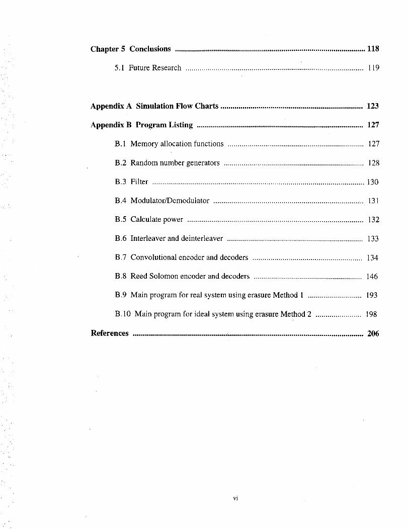
Chapter 5 Conclusions ............................................................................................... 118
5.1 Future Research ......................................................................................... 119
Appendix A Simulation Flow Charts ....................................................................... 123
Appendix B Program Listing ................................................................................... 127
B.1 Memory allocation functions .................................................................... 127
B.2 Random number generators ...................................................................... 128
B.3 Filter .......................................................................................................... 130
B.4 Modulator/Demodulator ......................................................................... ,. 131
B.5 Calculate power ........................................................................................ 132
B.6 Interleaver and deinterleaver .................................................................... 133
B.7 Convolutional encoder and decoders ....................................................... 134
B.8 Reed Solomon encoder and decoders ...................................................... 146
B.9 Main program for real system using erasure Method 1 ........................... 193
B. 10 Main program for ideal system using erasure Method 2 ....................... 198
References ............................................... _................................................................... 206
vi
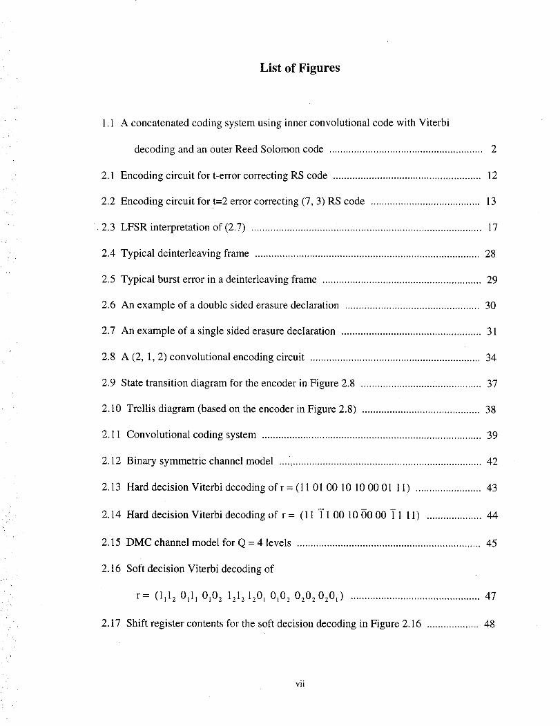
List of Figures
1.1 A concatenated coding system using inner convolutional code with Viterbi
decoding and an outer Reed Solomon code ........................................................ 2
2.1 Encoding circuit for t-error correcting RS code ...................................................... 12
2.2 Encoding circuit for t=2 error correcting (7, 3) RS code ........................................ 13
• 2.3 LFSR interpretation of (2.7)
2.4 Typical deinterleaving frame
.......................................... ° ......................................... 17
.................. ° .................. ° .................. • ......................... 28
2.5 Typical burst error in a deinterleaving frame .......................................................... 29
2.6 An example of a double sided erasure declaration ................................................. 30
2.7 An example of a single sided erasure declaration ................................................... 31
2.8 A (2, 1, 2) convolutional encoding circuit .............................................................. 34
2.9 State transition diagram for the encoder in Figure 2.8 37
2.10 Trellis diagram (based on the encoder in Figure 2.8) ........................................... 38
2.11 Convolutional coding system ................................................................................ 39
2.12 Binary symmetric channel model 42
2.13 Hard decision Viterbi decoding of r = (11 01 00 10 10 00 01 11) ........................ 43
2.14 Hard decision Viterbi decoding of r = (11 T 1 00 10 O0 00 T 1 11) .................... 44
2.15 DMC channel model for Q = 4 levels ................................................................... 45
2.16 Soft decision Viterbi decoding of
r= (1112 0111 0102 1212 1201 0102 0202 0201) ............................................... 47
2.17 Shift register contents for the soft decision decoding in Figure 2.16 ................... 48
vii
L
• _i_i_
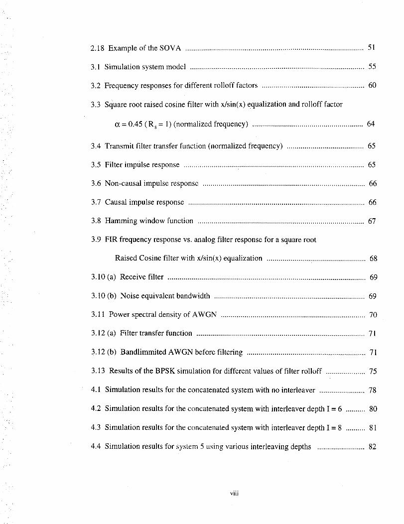
2.18 Example of the SOVA .......................................................................................... 51
3.1 Simulation system model ........................................................................................ 55
3.2 Frequency responses for different rolloff factors .................................................... 60
3.3 Square root raised cosine filter with x/sin(x) equalization and rolloff factor
= 0.45 (R s = 1) (normalized frequency) ........................................................ 64
3.4 Transmit filter transfer function (normalized frequency) ....................................... 65
3.5 Filter impulse response ........................................................................................... 65
3.6 Non-causal impulse response .................................................................................. 66
3.7 Causal impulse response ......................................................................................... 66
3.8 Hamming window function .................................................................................... 67
3.9 FIR frequency response vs. analog filter response for a square root
Raised Cosine filter with x/sin(x) equalization .................................................. 68
3.10 (a) Receive filter .................................................................................................... 69
3.10 (b) Noise equivalent bandwidth ............................................................................ 69
3.11 Power spectral density of AWGN ......................................................................... 70
3.12 (a) Filter transfer function ..................................................................................... 71
3.12 (b) Bandlimmited AWGN before filtering ............................................................ 71
3.13 Results of the BPSK simulation for different values of filter rolloff .................... 75
4.1 Simulation results for the concatenated system with no interleaver ....................... 78
4.2 Simulation results for the concatenated system with interleaver depth I = 6 .......... 80
4.3 Simulation results for the concatenated system with interleaver depth I = 8 .......... 81
4.4 Simulation results for system 5 using various interleaving depths ........................ 82
viii
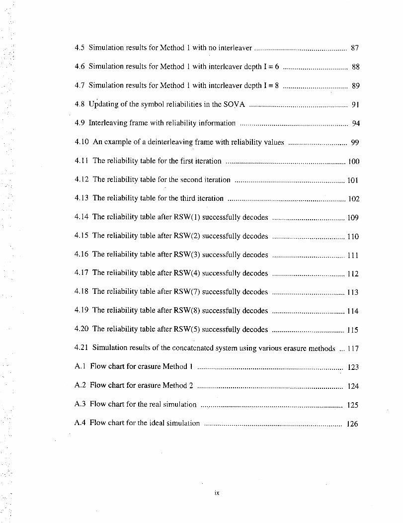
4.5
4.6
4.7
4.8
4.9
4.10
4.11
4.12
4.13
4.14
4.15
Simulation results for Method 1 with no interleaver ............................................... 87
Simulation results for Method 1 with interleaver depth I = 6 ................................. 88
Simulation results for Method 1 with interleaver depth I = 8 ................................. 89
Updating of the symbol reliabilities in the SOVA .................................................. 91
Interleaving frame with reliability information ....................................................... 94
An example of a deinterleaving frame with reliability values .............................. 99
The reliability table for the first iteration ............................................................. 100
The reliability table for the second iteration ........................................................ 101
The reliability table for the third iteration ............................................................ 102
The reliability table after RSW(1) successfully decodes ..................................... 109
The reliability table after RSW(2) successfully decodes ..................................... 110
4.16 The reliability table after RSW(3) successfully decodes ..................................... 111
4.17 The reliability table after RSW(4) successfully decodes ..................................... 112
4.18 The reliability table after RSW(7) successfully decodes ..................................... 113
4.19
4.20
4.21
A.1
A.2
A.3
A.4 Flow chart for the ideal simulation
The reliability table after RSW(8) successfully decodes ..................................... 114
The reliability table after RSW(5) successfully decodes ..................................... 115
Simulation results of the concatenated system using various erasure methods ... 117
Flow•chart for erasure Method 1 .......................................................................... 123
Flow chart for erasure Method 2 .......................................................................... 124
Flow chart for the real simulation .... .................................................................... 125
...................................................................... 26
ix

List of Tables
2.1 List of primitive polynomials for m = 3 to 9 ............................................................ 8
2.2 Three representations for the elements of GF(8) generated by 1 + x + x 3 ............ 9
2.3 Shift register contents for the encoding of u = [ o_ c_5 c_3 ] ................................ 14
2.4 Results of the computations for each iteration of the
Berlekamp-Massey algorithm ............................................................................ 21
2.5 Results of the computations for each iteration of the errors and erasures
Berlekamp-Massey algorithm ............................................................................ 25
2.6 Encoding of the information sequence u = (1 0 1 1 0 1) ......................................... 36
2.7 Development of the state diagram .......................................................................... 37
2.8 Conditional probabilities for BSC ..., ...................................................................... 42
2.9 Metric table for BSC ................................................................................................ 43
2.10 Conditional probabilities for DMC ............................... '........................................ 46
2.11 Metric table for DMC . .......................................................................................... 46
4.1 Various systems simulated ..................................................................................... -77
4.2 Simulation results using Method 2 with interleaving depth I = 8 .......................... 103
4.3 Simulation results using Method 3 with interleaving depth I = 8 .......................... 116
i, ¸
41."
Chapter 1
Introduction
Concatenated coding systems are often used for forward error correction to obtain
large coding gains when transmitting information over unreliable channels. One of the
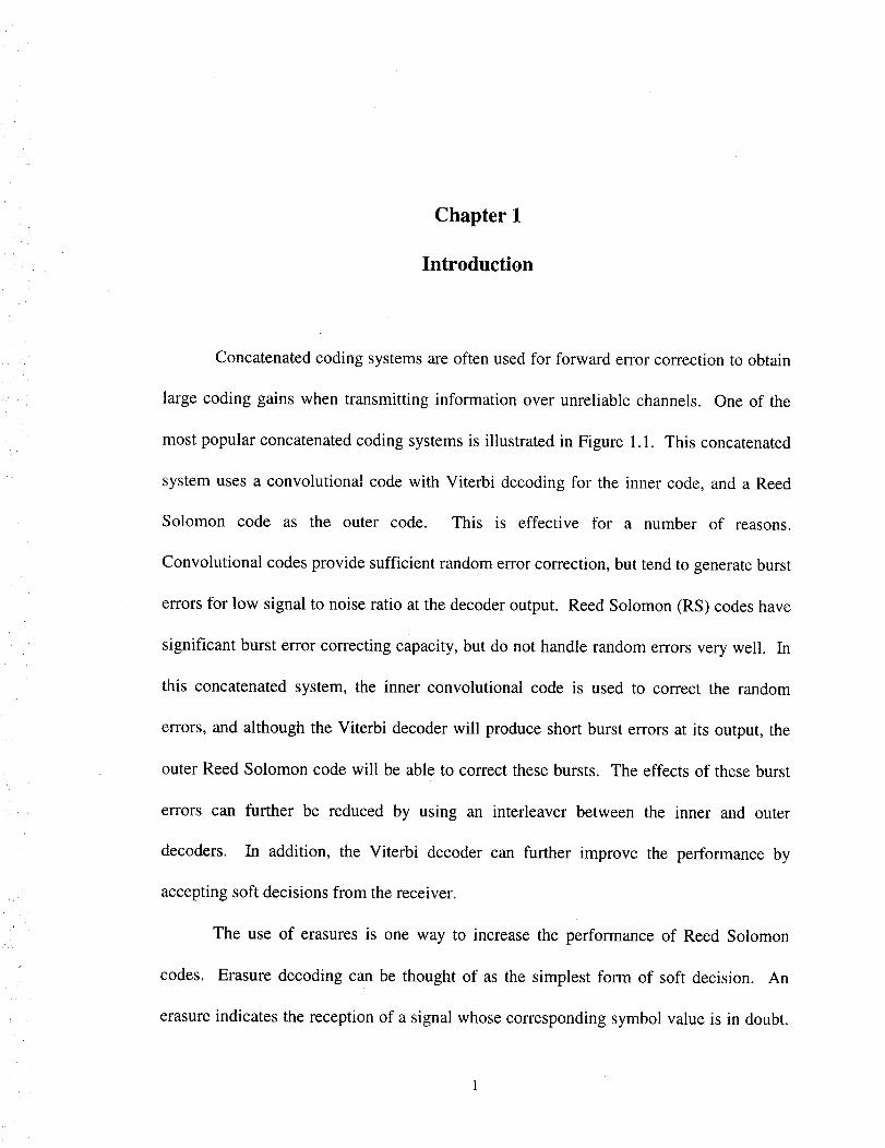
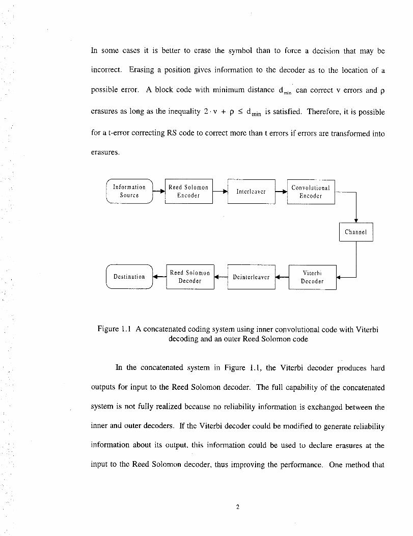
most popular concatenated coding systems is illustrated in Figure 1.1. This concatenated
system uses a convolutional code with Viterbi decoding for the inner code, and a Reed
Solomon code as the outer code. This is effective for a number of reasons.
Convolutional codes provide sufficient random error correction, but tend to generate burst
errors for low signal to noise ratio at the decoder output. Reed Solomon (RS) codes have
significant burst error correcting capacity, but do not handle random errors very well. In
this concatenated system, the inner convolutional code is used to correct the random
errors, and although the Viterbi decoder will produce short burst errors at its output, the
outer Reed Solomon code will be able to correct these bursts. The effects of these burst
errors can further be reduced by using an interleaver between the inner and outer
decoders. In addition, the Viterbi decoder can further improve the performance by
accepting soft decisions from the receiver.
The use of erasures is one way to increase the performance of Reed Solomon
codes. Erasure decoding can be thought of as the simplest form of soft decision. An
erasure indicates the reception of a signal whose corresponding symbol value is in doubt.
In somecasesit is better to erasethe symbol than to force a decision that may be
incorrect. Erasing a position gives information to the decoderas to the location of a
possibleerror. A block code with minimum distancedm_° cancorrect v errorsand 9
erasures as long as the inequality 2. v + p _< dmi n is satisfied. Therefore, it is possible
for a t-error correcting RS code to correct more than t errors if errors are transformed into
erasures.
IInformation___ ReedSolomon _ ___ ConvolutionalSource Encoder Interleaver Encoder
Channel
IDestinati°n _-_ ReedS°_°m°n _ Deinterleaver_--_. Decoder DecoderViterbi ___
Figure 1.1 A concaienated coding system using inner ¢olavolutional code with Viterbi
decoding and an outer Reed Solomon code
In the concatenated system in Figure 1.1, the Viterbi decoder produces hard
outputs for input to the Reed Solomon decoder. The full capability of the concatenated
system is not fully realized because no reliability information is exchanged between the
inner and outer decoders. If the Viterbi decoder could be modified to generate reliability
information about its output, this information could be used to declare erasures at the
input to the Reed Solomon decoder, thus improving the performance. One method that
2

can be used to accomplish this is the Soft Output Viterbi Algorithm (SOVA). The
method proposed by Hagenauer and Hoeher [4] uses information provided by the path
metrics in the Viterbi decoder to determine a reliability value associated with each
outgoing bit.
One application where this gain could be potentially useful is in NASA deep
space missions. The transmission of data over large distances, combined with limited
transmission power, results in low signal to noise ratio at the receiving end. This,
coupled with the fact that the data being transmitted is in the form of compressed images
where the required probability of error is 10 .5 , leads to the need for a powerful coding
system [16]. The NASA standard for deep space communications is the (255, 223) 16
error correcting RS code as the outer code, and the rate 1/2 convolutional code with
constraint length K = 7. Interleaver depths of I = 2 to 8 have been used. The use of a
SOVA and an errors and erasures RS decoder can provide additional gains with no need
to modify the transmitting end. This enables erasure decoding to be used in existing
missions. This is particularly helpful for missions where unforeseen problems occur.
The Galelaio mission where the main antenna failed is one such instance. Every tenth of
a decibel gain that can be obtained in this instance is extremely helpful [15].
One method used to improve the NASA standard for deep space communications
through the use of erasures has been investigated by Paaske [7]. This method uses the
deinterleaver to provide information concerning the probable locations of errors in non-
decoded Reed Solomon codewords in an interleaving frame. In an deinterleaving flame
there are I Reed Solomon codewords, where I is the interleaving depth, ff after
attempting to decode the frame, some of the RS codewords fail to decode, redecoding is
used. Erasures are declared using information provided by the error positions in the
successfully decoded RS codewords. Because the Viterbi decoder produces burst of
errors at it's output, and the data is fed into the deinterleaver by row and output by
column to the Reed Solomon decoder, the bursts occur at the same symbols in
neighboring Reed Solomon words in the deinterleaver frame. If some but not all of the
Reed Solomon words in the deinterleaving frame have been successfully decoded, the
positions of the errors in the decoded words are known. The knowledge of the error
positions can be used to declare erasures in the same positions in neighboring, yet to be
decoded Reed Solomon codewords.
1.1 Proposed research
The purpose of this report is to investigate the performance of the use of a Soft
Output Viterbi Algorithm used in a concatenated coding scheme with an errors and
erasures RS decoder. The reliability information provided by the SOVA will be
converted into Reed Solomon symbol erasures for the RS decoder. A table of least
reliable symbols will be compiled for each RS codeword, and systematically erased. In
addition, another method loosely based upon Paaske's method will be investigated. This
method combines the SOVA output with a deinterleaver. The table of least reliable
symbols •can be modified using additional information provided by the deinterleaver. If
after the first decoding of a deinterleaving frame, there are less than I successful decoding
of RS codewords, redecoding is attempted. It turns out that not only does the SOVA
outputproducebursterrors,but thereliabilitiesfor theseerror symbolsareidentical. This
informationis usedto modify thetableof smallestreliabilities. Theperformanceof these
codeswill be obtainedthroughtheuseof a computersimulationwritten in C computer
language. The convolutional code developedfor use in this simulation is capableof
handling any code rate and constraintlength. The Reed Solomoncode, likewise, can
handle any symbol size and numberof symbol errorscorrected. The ReedSolomon
• decoderis anerrorsanderasuresdecoder. Althoughthe codesdevelopedarecapableof
handling any size code, the NASA standardcoding systemwill be investigatedwith
various interleavingdepths. The simulationwill be performedover a AWGN channel
usingBPSK modulationandRaisedCosineFIR filters. Thecodingsystemswill alsobe
simulatedoveranidealBPSKchannel.
Thestructureof this reportis asfollows. Chapter2 containsall of thebackground
information. Chapter3 will containthe detailsof thecomputersimulation. Chapter4
will containthe strategyfor declaringRSsymbolerasuresfrom thereliability information
generatedby the SOVA, andthestrategyfor usingtheSOVA with thedeinterleaverfor
redecoding. Chapter4 will alsopresentthe resultsof the simulationfor both methods
investigated.Chapter5 will containconclusions,andideasfor possiblefuture research.
Thesimulationflow chartsarefoundin AppendixA andtheC languagesourcecodeused
tOperform thesimulationscanbefoundin AppendixB.


.i- 4
Chapter 2
Background
Before discussing the two methods for erasure declaration presented in this report,
it is helpful to become familiar with some of the basic concepts of error control codes.
This chapter will contain all of the background necessary to understand the various
elements used in the concatenated system. Encoding and decoding of Reed Solomon and
convolutional codes will be reviewed. In addition, the method used for errors and
erasures decoding in the Reed Solomon decoder will be discussed, as well as the method
used for generating the soft outputs in the Viterbi decoder. Block interleaving will be
briefly discussed, in addition to the redecoding method proposed by Paaske.
2.1 Reed Solomon codes
Bose-Chadhuri-Hocquenghem (BCH) codes are a powerful class of cyclic codes
which outperform all other block codes with the same block length and code length [9].
These codes are a generalization of Hamming codes to allow multiple error correction.
Reed Solomon (RS) codes are special subclass of BCH codes which utilize non-binary
symbols. The non-binary symbols used in RS codes are formed using finite field
arithmetic. Finite fields are sometimes called Galois fields and are denoted by GF(p),
where p is the number of elements in the field, and is a prime number.
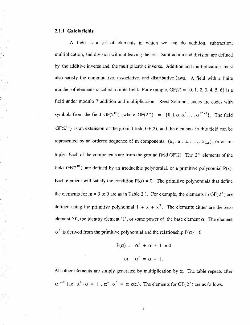
2.1.1 Galois fields
A field is a set of elements in which we can do addition, subtraction,
multiplication, and division without leaving the set. Subtraction and division are defined
by the additive inverse and the multiplicative inverse. Addition and multiplication must
also satisfy the commutative, associative, and distributive laws. A field with a finite
number of elements is called a finite field. For example, GF(7) = {0, 1, 2, 3, 4, 5, 6} is a
field under modulo 7 addition and multiplication.
symbols from the field GF(2m), where GF(2 m)
Reed Solomon codes are codes with
= {0,1,_,o_ 2 ..... (_2m-2}. The field
GF(2 m) is an extension of the ground field GF(2), and the elements in this field can be
represented by an ordered sequence of m components, (a0, a_, a z ..... am. l), or an m-
tuple. Each of the components are from the ground field GF(2). The 2 m elements of the
field GF(2 m) are defined by an irreducible polynomial, or a primitive polynomial P(x).
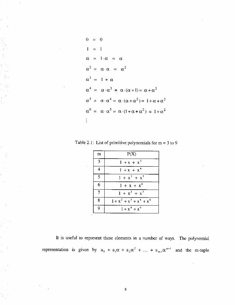
Each element will satisfy the condition P(cz) = 0. The primitive polynomials that define
the elements for m = 3 to 9 are as in Table 2.1. For example, the elements in GF(2 3) are
defined using the primitive polynomial 1 + x + x 3 . The elements either are the zero
element '0', the identity element ' 1', or some power of the base element or. The element
o_3 is derived from the primitive polynomial and the relationship P(cz) = 0.
P(00= o_3 + _ + 1 =0
or ot 3 =c_+ 1.
All other elements are simply generated by multiplication by or. The table repeats after
o_m-2 (i.e. o_6 • o_ = 1 , o_6 •o_2 = o: etc.). The elements for GF(23 ) are as follows.
0 = 0
1 = 1
(2 = 1"_ = (2
(22 = (2.(2 = (22
(X 3 = 1+(2
(24 = (2.(23 = (2"((2+1)= (2+(22
(25 = (2.(24= (2.((2+(22)= 1+(2+(22
(26 = (2.(25= (2.(1+(2+052) = 1+(22
Table 2.1: List of primitive polynomials for m = 3 to 9
m P(X)
3 1 +X+X 3
4 1 +X +X 4
5 1 + x 2 + x 5
• 6 1 +X+X 6
7 1 + x 3 + x 7
8 l+x 2 ..i,- X 3 ..{-X 4 ,.[.- X 8
9 l+x 4 -I-X 9
It is useful to represent these elements in a number of ways. The polynomial
(2m-Irepresentation is given by a 0 + a_(2 + a2(2 2 + ... + am. 1 and the m-tuple
)
representation is given by (a o, a l, a 2..... am.l).
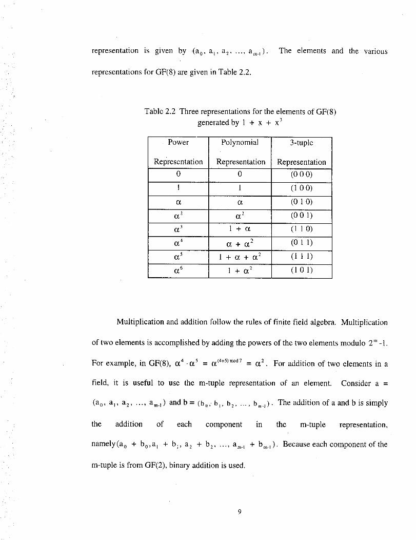
representations for GF(8) are given in Table 2.2.
The elements
Table 2.2 Three representations for the elements of GF(8)3
generated by 1 + X + x
Power Polynomial 3-tuple
Representation Representation Representation
0 0 (0 0 0)
1 1 (1 oo)
a c_ (0 1 0)
_: ot2 (0 0 1)
_3 1 + _ (1 10)
_4 a + _2 (0 1 1)
_5 1 -I- (_ "t" 0_ 2 (1 1 1)
(_6 1 + o_2 (1 0 1)
and the various
Multiplication and addition follow the rules of finite field algebra. Multiplication
of two elements is accomplished by adding the powers of the two elements modulo 2 m_1.
For example, in GF(8), (x4 .0_ 5 = a(4+5)mod7 = 0_2. For addition of two elements in a
field, it is useful to use the m-tuple representation of an element. Consider a =
(a o, a_, a 2..... am.l) andb = (b,,, b_, b2 ..... bin,)" The addition of a and b is simply
the addition of each component
namely(a o + bo,a t + b_, a 2 + b 2 ..... am. l
m-tuple is from GF(2), binary addition is used.
in the m-tuple representation,
+ bm. 1 ). Because each component of the
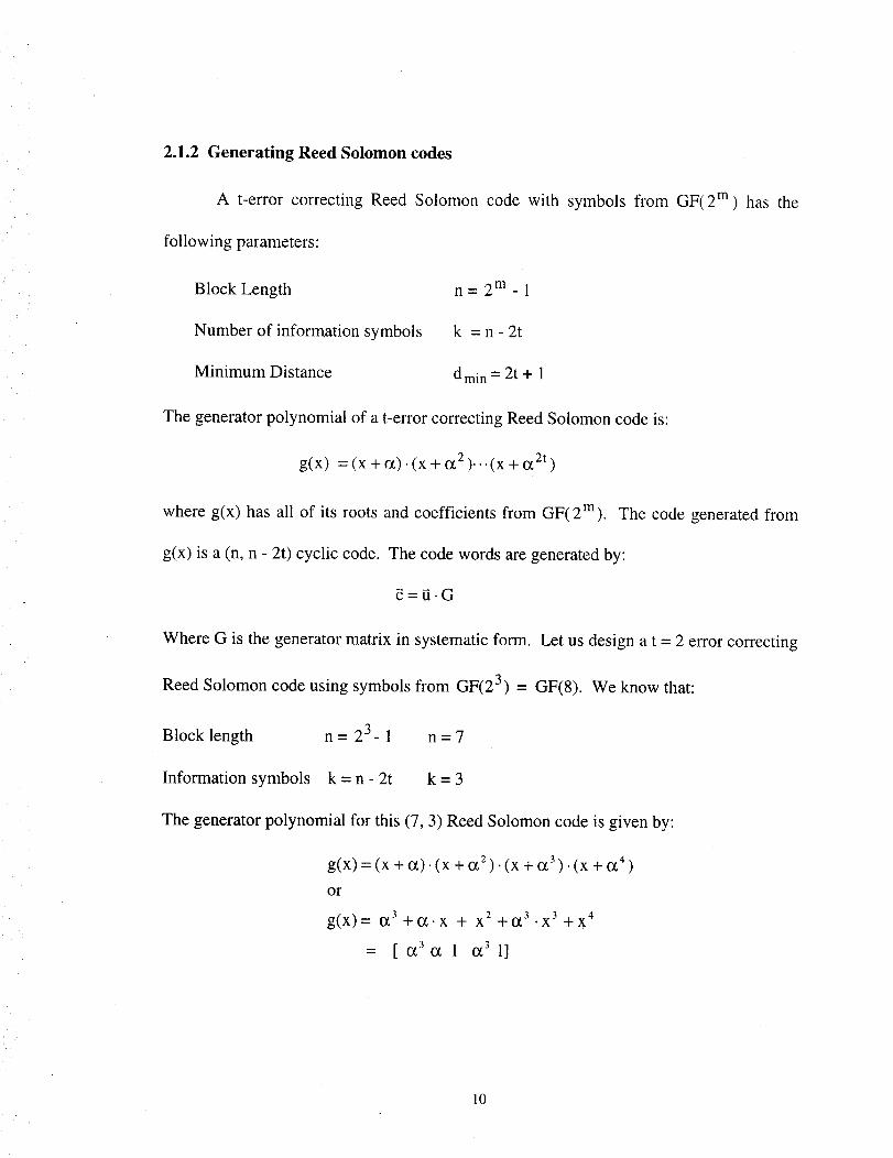
2.1.2 Generating Reed Solomon codes
A t-error correcting Reed Solomon code with symbols from GF(2 m) has the
following parameters:
Block Length n = 2 m - 1
Number of information symbols k = n - 2t
Minimum Distance dmi n = 2t + 1
The generator polynomial of a t-error correcting Reed Solomon code is:
g(x) = (x + or). (x + cx 2 )'" "(X + O_2t )
where g(x) has all of its roots and coefficients from GF(2m). The code generated from
g(x) is a (n, n - 2t) cyclic code. The code words are generated by:
_=_.G
Where G is the generator matrix in systematic form. Let us design a t - 2 error correcting
Reed Solomon code using symbols from GF(2 3) - GF(8). We know that:
Block length n = 2 3- 1 n = 7
Information symbols k = n - 2t k = 3
The generator polynomial for this (7, 3) Reed Solomon code is given by:
g(x) = (x + or)(x + c_, 2 ). (x --_ 0(, 3 ). (x + 0_, 4 )
or
g(x)= _3 +cz.x + x 2 +cz 3 .x 3 -[-X 4
= [ 0_30_ 1 o_3 1]
10
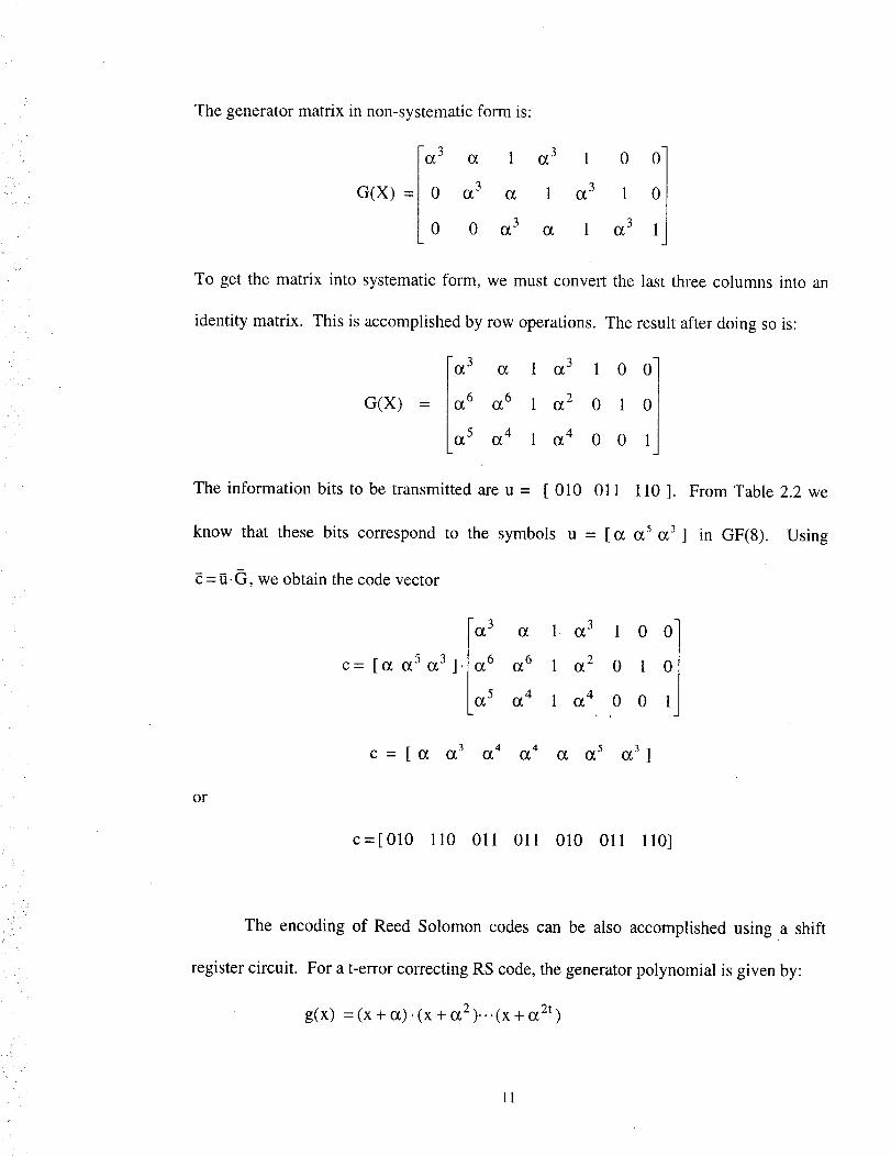
Thegeneratormatrix in non-systematicform is:
G(X) = 0 o_3 c_ 1 o_3 1
0 0 o_3 _ 1 ot3
To get the matrix into systematicform, we mustconvert the last threecolumnsinto an
identity matrix. This is accomplishedby rowoperations.Theresultafterdoingsois:
G(X) = O_6 O_6 1 _2 0 1
(Z 5 O_4 1 _4 0 0
The information bits to be transmitted are u = [ 010 011 110 ]. From Table 2.2 we
know that these bits correspond to the symbols u = [c_ o_5 c_3 ] in GF(8). Using
c = g.CJ, we obtain the code vector
= . _6 0_6 _2c [or o_5 o_3 ] 1 0 1
0_5 _4 10_ 4 0 0
C "- [ I_ I_ 3 0_ 4 1_4 1_ 1_5 1_3 ]
or
C=[010 110 011 011 010 011 110]
_i. ¸" .
i/•
The encoding of Reed Solomon codes can be also accomplished using a shift
register circuit. For a t-error correcting RS code, the generator polynomial is given by:
g(x) = (x + _). (x + _2 ).. "(X + O_2t )
11
=go + glx + g2 x2 + ... + g2t.i x2t-I + X 2t
'%/,
where g(x) has all of its roots and has coefficients from GF(2m). The generator
polynomial g(x) has been chosen so that it and codewords generated by it have zeros for
2. t consecutive powers of o_
g(c_ j) = 0 forj= 1,2 .... 2.t
The code generated from g(x) is a (n, n - 2t) cyclic code. The encoding of a non-binary
cyclic code is similar to the encoding of a binary cyclic code. Let
H(X)=U 0 "_- nix "[" U2 X2 "l- "'" "1"- U2t.l x2t-I
be the message to be encoded. In systematic form, the 2t parity check symbols are the
coefficients of the remainder b(x)=b 0 + blX 4" b2 x2 4- .-. 4- b2t.1 x2t-I which is
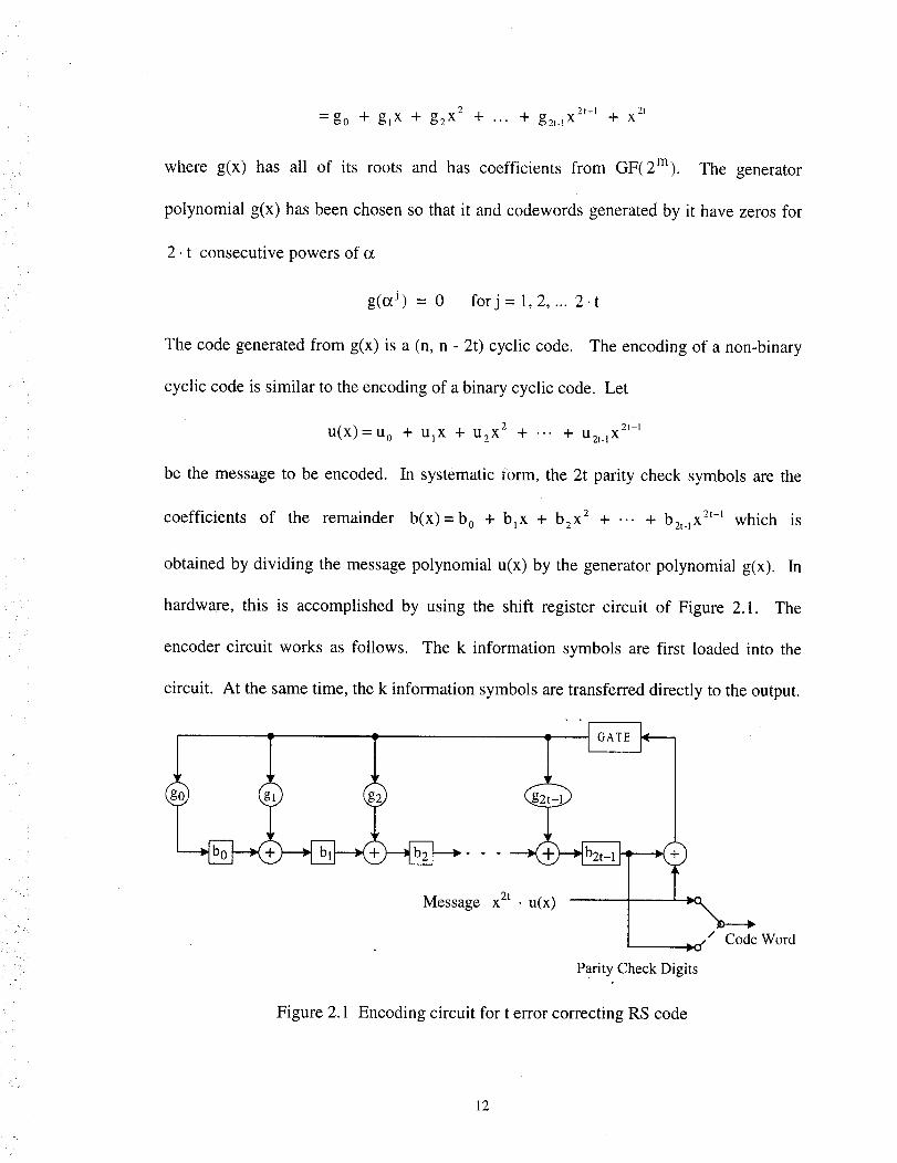
obtained by dividing the message polynomial u(x) by the generator polynomial g(x). In
hardware, this is accomplished by using the shift register circuit of Figure 2.1. The
encoder circuit works as follows. The k information symbols are first loaded into the
circuit. At the same time, the k information symbols are transferred directly to the output.
r
Message X 2t" U(X)
_..,_/ Code Word
Parity Check Digits
Figure 2.1 Encoding circuit for t error correcting RS code
12
Whenall of the informationsymbolshavebeenreadin, the2t parity symbolsarepresent
in the 2t registersdenotedb0, b_..... bzt. ] , and are then transferred to the output, thus
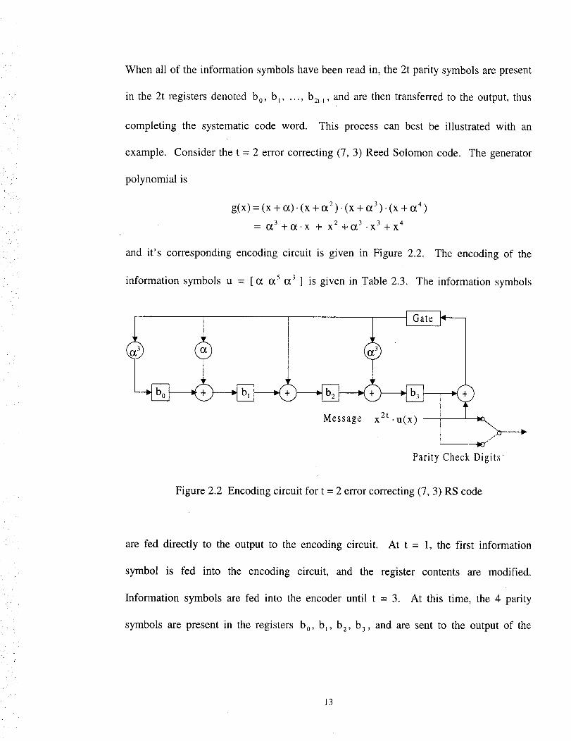
completing the systematic code word. This process can best be illustrated with an
example. Consider the t = 2 error correcting (7, 3) Reed Solomon code. The generator
polynomial is
g(x) = (x + c_). (x + _2 ). (x + 0_3) • (x + (_4)
= (_3 ..{._(_. X -{'- X 2 -1-(_3 . X 3 _{_ X 4
and it's corresponding encoding circuit is given in Figure 2.2. The encoding of the
information symbols u = [c_ _5 o_3 ] is given in Table 2.3. The information symbols
'I
r
Message
_O r
r r
X 2t "U(X)
)
Parity Check Digits
Figure 2.2 Encoding circuit for t = 2 error correcting (7, 3) RS code
are fed directly to the output to the encoding circuit. At t = 1, the first information
symbol is fed into the encoding circuit, and the register contents are modified.
Information symbols are fed into the encoder until t = 3. At this time, the 4 parity
symbols are present in the registers b 0, b l, b 2, b3, and are sent to the output of the
13
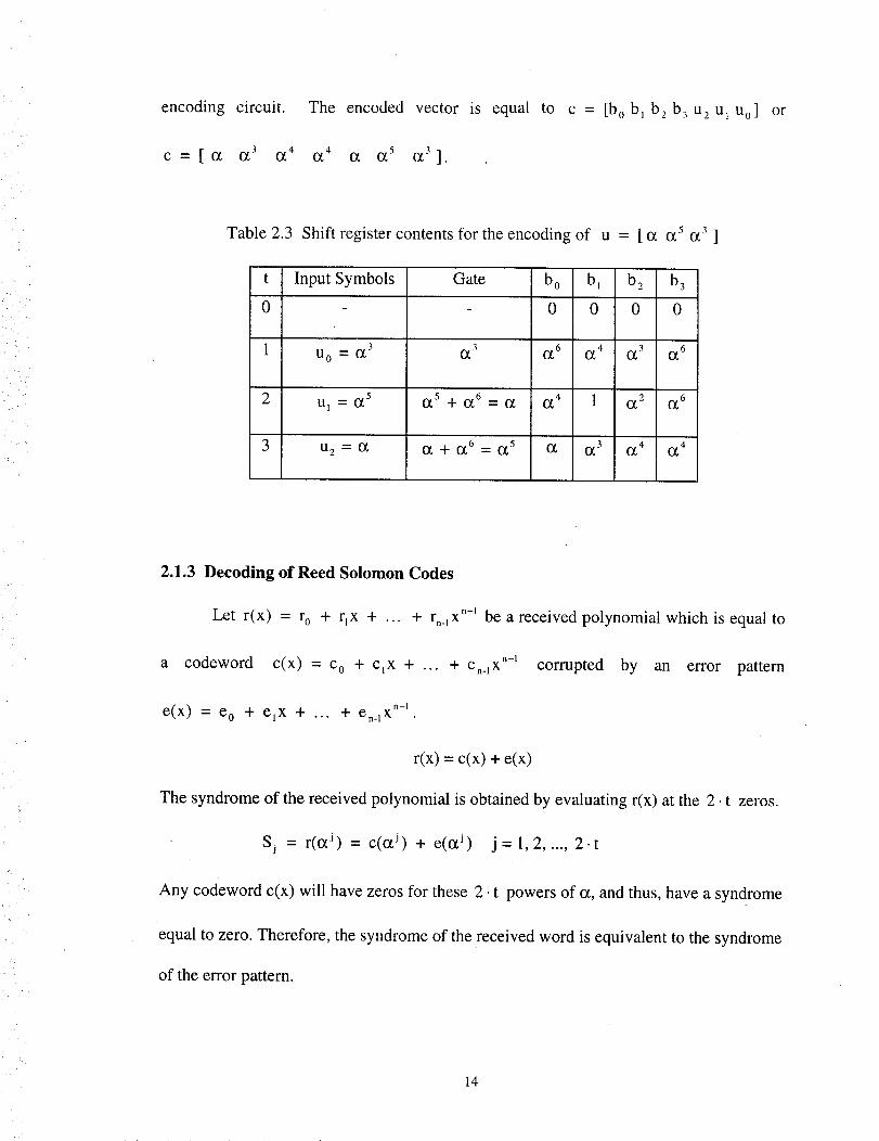
The encoded vector is equal to
_4 _ _5 _3].
c = [b o b I b 2 b 3 U 2 UI UO] or
Table 2.3 Shift register contents for the encoding of u = [ (z o_5 o_3 ]
; (. ( i
t
0
Input Symbols Gate
U 0 = O_3 0(, 3
bo bl b 2 b 3
0 0 0 0
_6 _4 _3 _6
2.1.3 Decoding of Reed Solomon Codes
Let r(x) = r0 + q x + ... + r.._x n-I be a received polynomial which is equal to
a codeword c(x) = C O "1" ClX de.....1_ Cn.l xn-I corrupted by an error pattern
n-Ie(x) = e o + e_x + ... + en.lX .
r(x) = c(x) + e(x)
The syndrome of the received polynomial is obtained by evaluating r(x) at the 2. t zeros.
Sj = r(&) = c(_ j) + e(&) j=l,2 ..... 2.t
Any codeword c(x) will have zeros for these 2. t powers of a, and thus, have a syndrome
equal to zero. Therefore, the syqdrome of the received word is equivalent to the syndrome
of the error pattern.
14
n-I
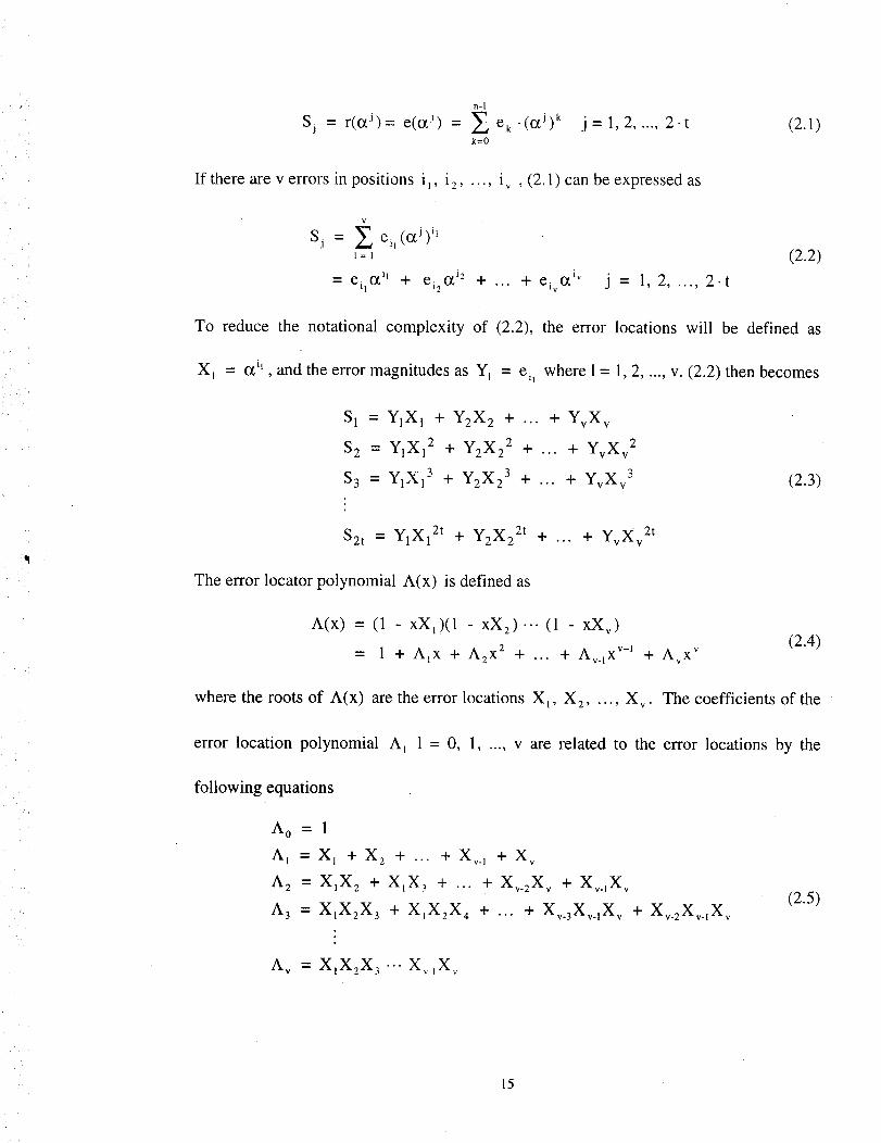
Sj = r((zJ): e((z j) -- £ e k "(o{,J) k j= 1,2 ..... 2.t (2.1)
k=0
If there are v errors in positions i j, i 2 ..... i v , (2.1) can be expressed as
Sj = _ eij(_J) il
1= l (2.2)
= eq(X q + ei20{, j2 + ... + eiv(X _v j = 1,2 ..... 2.t
To reduce the notational complexity of (2.2), the error locations will be defined as
X_ = cz '_ , and the error magnitudes as Y_ = e_, where 1 = 1, 2 ..... v. (2.2) then becomes
S 1 = YIXl + Y2X2 + ... + YvXv
S 2 = YIX12 + YzX2 2 + ... + YvXv 2
3S 3 = Y1X1 + YzX2 3 + ... + YvXv 3
2t 2tSzt -- Y1Xl + YzX2 + ... + YvXv 2t
(2.3)
The error locator polynomial A(x) is defined as
A(x) = (1 - xX,)(1 - xX2)... (1 - xXv)
= 1 + A_x + A2 x2 + ... + Av._X v-_ + Av xv(2.4)
where the roots of A(x) are the error locations X_, X 2 ..... X v . The coefficients of the
error location polynomial A_ 1 = 0, 1..... v are related to the error locations by the
following equations
Ao=l
A_ = X_ + X 2 + ... + Xv._ + Xv
A 2 = XlX 2 + XIX 3 + ... + X__2X _ + X_.IX _
A 3 = XIX2X 3 + XIX2X 4 + ... + X_.3Xv.IX v + Xv.2X__IX _(2.5)
A v = XlX2X 3 ... Xv_lX v
15
L• _i
i
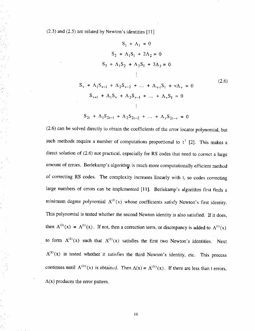
(2.3) and (2.5) are related by Newton's identities [11]
S 2
S 3 + A1S 2 + A2S 1
S v + A1Sv_ 1 + AzSv_ 2 + ...
S 1 + A 1 = 0
+ AIS 1 + 2A 2 = 0
+ 3A 3 = 0
+ Av.lS 1 + vA v = 0(2.6)
Sv+l + A1Sv + A2Sv_ 1 + ... + AvS l = 0
S2t + A1S2t_I + A2S2t_ 2 + ... + AvS2t_ v = 0
(2.6) can be solved directly to obtain the coefficients of the error locator polynomial, but
such methods require a number of computations proportional to t 3 [2]. This makes a
direct solution of (2.6) not practical, especially for RS codes that need to correct a large
amount of errors. Berlekamp's algorith_ is much more computationally efficient method
of correcting RS codes• The complexity increases linearly with t, so codes correcting
large numbers of errors can be implemented [11]. Berlekamp's algorithm first finds a
minimum degree polynomial A(*_(x) whose coefficients satisfy Newton's first identity.
This polynomial is tested whether the second Newton identity is also satisfied. If it does,
then A(2)(x) = A(_(x). If not, then a correction term, or discrepancy is added to A(l)(x)
to form A(2_(x) such that A(2_(x) satisfies the first two Newton's identities. Next
A(2)(x) is tested whether it satisfies the third Newton's identity, etc. This process
continues until A (2'_(x) is obtained. Then A(x) = A (2'_(x). If there are less than t errors,
A(x) produces the error pattern.
16
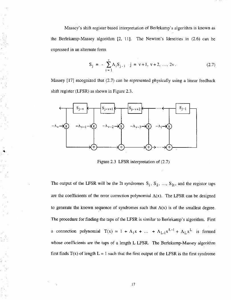
Massey's shift register based interpretation of Berlekamp's algorithm is known as
the Berlekamp-Massey algorithm [2, 11]. The Newton's Identities in (2.6) can be
expressed in an alternate form
i-
:i /"
V
Sj = ZAiSj.i j = v+l, v+2 ..... 2v. (2.7)i=l
Massey [17] recognized that (2.7) can be represented physically using a linear feedback
shift register (LFSR) as shown in Figure 2.3.
-Av-l"" _ ) -Av-2-'-_ _Av_3_..)Q
) ,(
) -A1---X
Figure 2.3 LFSR interpretation of (2.7)
The output of the LFSR will be the 2t syndromes S 1, S 2 ..... S2t, and the register taps
are the coefficients of the error correction polynomial A(x). The LFSR can be designed
to generate the known sequence of syndromes such that A(x) is of the smallest degree.
The procedure for finding the taps of the LFSR is similar to Berlekamp's algorithm. First
a connection polynomial T(x) = 1 + mix + ...
whose coefficients are the taps of a length L LFSR.
+ AL.lXL-I+ AL xL is formed
The Berlekamp-Massey algorithm
first finds T(x) of length L = 1 such that the first output of the LFSR is the first syndrome
17
2
S l . The second output of the LFSR is compared to the second syndrome, and if the two
are not equal then the connection polynomial is modified using a discrepancy term. If the
two are equal the taps remain the same. The third output of the LFSR is compared to the
third syndrome, and if they are not equal, the taps of the connection polynomial are
modified. This process continues for 2t iterations. At the end of the 2t iterations, the taps
of the LFSR specify the coefficients of the error correction polynomial A(x). The details
of the algorithm are presented below.
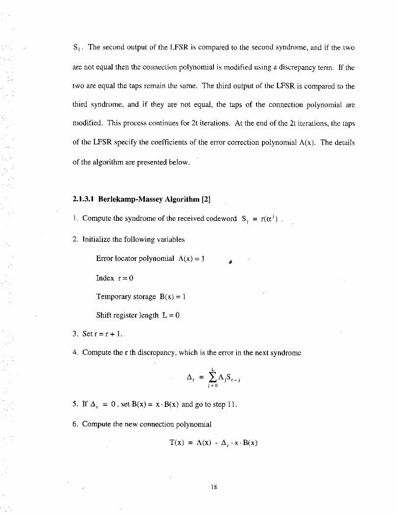
2.1.3.1 Berlekamp-Massey Algorithm [2]
1. Compute the syndrome of the received codeword Sj = r(od) .
. Initialize the following variables
Error locator polynomial A(x) = 1
Index r = 0
8•
.
Temporary storage B(x) = 1
Shift register length L = 0
Setr=r+ 1.
. Compute the r th discrepancy, which is the error in the next syndrome
L
m r = 2AjSr_j
j=0
5. If A r = 0, setB(x) = x.B(x) and go to step 11.
6. Compute the new connection polynomial
T(x) = A(x) - A r .x.B(x)
18
7. If 2-L > r - 1,setB(x)= x.B(x) andgoto step10.
8. Storeold shift registerafternormalizing
B(x) = Ar-'A(x )
9. Updateshift registerlength L = r - L.
10. Updatetheshift register
A(x) = T(x)
11. If r< 2.t,gotostep3.
12. If deg A(x) _: L, there are more than t errors. Stop.
13. Determine the roots of A(x). The inverses of these roots are the error locations
Xl, X2 ..... X v •
14. Determine the corresponding error values YI, Y2 ..... Yr.
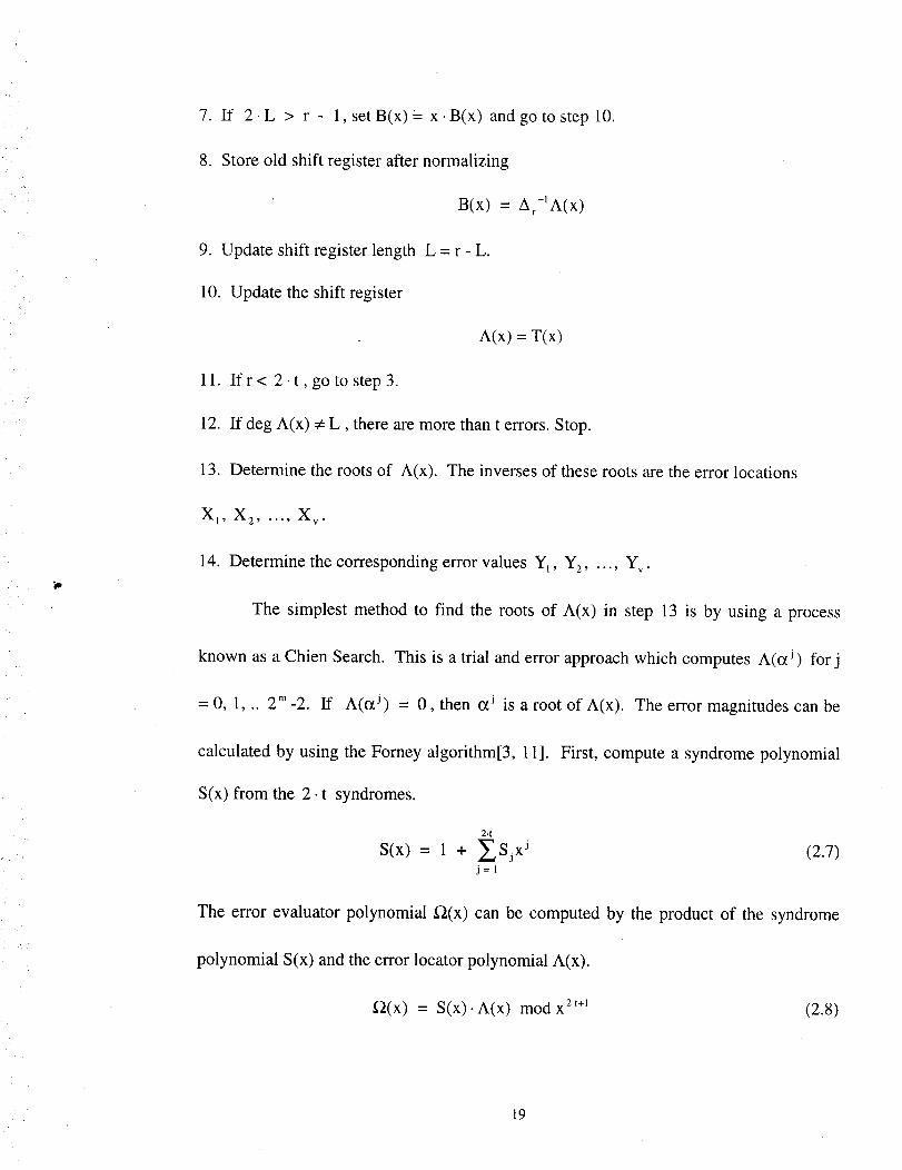
The simplest method to find the roots of A(x) in step 13 is by using a process
known as a Chien Search. This is a trial and error approach which computes A(c_ j) for j
= 0, 1, .. 2 m-2. If A(0_ j) = 0, then o_j is a root of A(x). The error magnitudes can be
calculated by using the Forney algorithm[3, 1 I]. First, compute a syndrome polynomial
S(x) from the 2. t syndromes.
2.t
S(x) = 1 + _[]Sjx j (2.7)j=l
The error evaluator polynomial f_(x) can be computed by the product of the syndrome
polynomial S(x) and the error locator polynomial A(x).
g_(x) = S(x). A(x) mod x 2'+] (2.8)
19
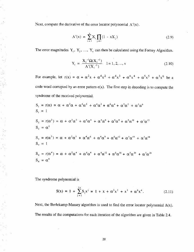
Next, compute the derivative Of the error locator polynomial A'(x).
A'(x) = £XiI"[(1 - xXj) (2.9)i=l j_i
The error magnitudes Y_, Y2 ..... Yv can then be calculated using the Forney Algorithm.
f
X 1 -I _"_(X 1-1 )
YI = 1 = 1, 2 ..... v (2.10)-1
A'(XI )
For example, let r(x) - c_ + 1_2x + _4x2 + o_4x 3 + (_6x4 + (_5x5 + o_3x 6 be a
code word corrupted by an error pattern e(x). The first step in decoding is to compute the
syndrome of the received polynomial.
S_ = r(a) = a + t_2t_ + 0_4('_2 dr" (_4(_3 "-I- (_60_4 -[- 0_50_5 -I- 0_3(_6
$1=1
S 2 -- r(_ 2) -" (X + (X2tX z + (_40_4 -st- (_4(_6 d- 0_,6C_,8 dt - 0_50_ 10 -1-- (_3(_12
S 2 = O_ 2
S 3 - r(_ 3) "- _ + 0_2_ 3 + 1_40_ 6 4" C/_4_9 "t - 13_,61_12 "Jr" 1_51_15 -I- C_31_18
83----1
S 4 -- r((X 4) = (X + 0_20_ 4 -_- (_41_8 dr- (_4(_,12 q. (_60_16 dr _50_20 q_ (_30_24
S 4 : 13(, 6
The syndrome polynomial is
2.t
S(x) = 1 + y__Sjx j =j=l
1 + x + c[,2x 2 -t- x 3 -+. o(,6x 4 . (2.11)
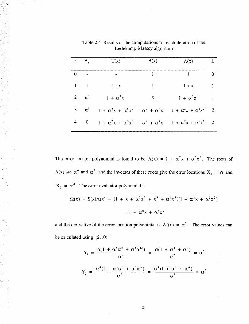
Next, the Berlekamp-Massey algorithm is used to find the error locator polynomial A(x).
The results of the computations for each iteration of the algorithm are given in Table 2.4.
2O
,i ¸ ,
Table 2.4 Results of the computations for each iteration of the
Berlekamp-Massey algorithm
r A r T(x) B(x) A(x) L
0 1 1 0
1 1 l+x 1 l+x 1
2 _6 1 + (22x x 1 + (22x 1
3 c_5 1 "4- (22X "[- (25X2 (23(,2 + (24X 1 + c_2x + _5x2 2
4 0 1 "_ (ff_2X "1"- {_5X2 1_2 -'1- [_4X 1 + _2x + c_Sx2 2
The error locator polynomial is found to be A(x) = 1 + (22X "t- (25X2. The roots of
A(x) are (26 and (23, and the inverses of these roots give the error locations X_ = (2 and
X2 = (24. The error evaluator polynomial is
_2(x) = S(x)A(x) = (1 + x + (22x2 + x 3 + 0_6x4)(1 + (22x + (25x2)
= 1 + O_.6X q" (_5X2
and the derivative of the error location polynomial is A'(x) = I_, 2 . The error values can
be calculated using (2.10)
y_ = (2(1 + (26(26 -I- (25(212) .._ (2(1 + (25 + (23) = (25(22 (22
(24(1 + (26(23 q_ (25(26) _ (24(1 + (22+ (24) = (25
Y2 = i._2 - (22
21
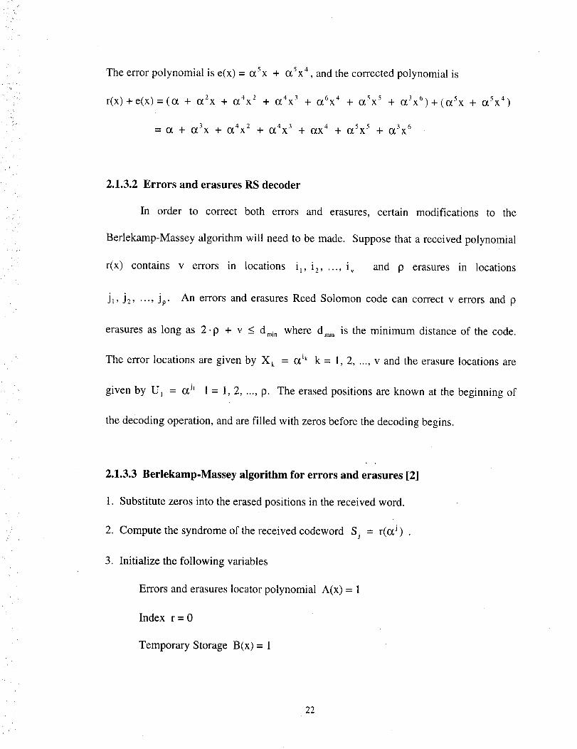
The error polynomial is e(x) = c_Sx + o_5x 4 , and the corrected polynomial is
r(x)+e(x)=(ot + _2x + c_4x 2 + 1_4x3 -st- o_6x 4 ..{- o_5x 5 -Jr- o_3x6)..t.-((_5x --I.- (ff_5x4)
--(_ -.I.- o_3x --I.- o_4x 2 .4- o_,4x 3 -.I- o_x 4 .._ o_5x 5 q.- (_3x6
2.1.3.2 Errors and erasures RS decoder
In order to correct both errors and erasures, certain modifications to the
Berlekamp-Massey algorithm will need to be made. Suppose that a received polynomial
r(x) contains v errors in locations i 1, i 2 ..... i v and 9 erasures in locations
Jl, J2 ..... Jp- An errors and erasures Reed Solomon code can correct v errors and 9
erasures as long as 2. 9 + v < dmin where dmi n is the minimum distance of the code.
The error locations are given by X k = o__k k = 1, 2 ..... v and the erasure locations are
given by U_ = o_j_ 1 = 1, 2 ..... 9. The erased positions are known at the beginning of
the decoding operation, and are filled with zeros before the decoding begins.
2.1.3.3 Berlekamp-Massey algorithm for errors and erasures [2]
1. Substitute zeros into the erased positions in the received word.
2. Compute the syndrome of the received codeword Sj = r(o0 )
3. Initialize the following variables
Errors and erasures locator polynomial A(x) = 1
Index r = 0
Temporary Storage B(x) = 1
22

Shift registerlength L = 0
4. Setr=r+l.
5. Ifr>p go to stepl0
6. A(x) = A(x).(1 - U r • X)
7. B(x) = A(x)
8. L=L+ 1
9. Go to step 4
10. Compute the r th discrepancy, which is the error in the next syndrome
L
A r = _AjSr_ jj=0
11. IrA = 0,setB(x)= x.B(x) and go to stepll.
12. Compute the new connection polynomial T(x) "- A(X) - A r • X" B(x)
13. If 2.L > r + P - 1, set B(x) = x.B(x) and go to step 16.
14. Store old shift register after normalizing
B(x) = Ar-lA(x)
15. Update shift register length L = r - L ÷ p.
16. Update the shift register
A(x) = T(x)
17. Ifr<2.t,gotostep4.
18. If deg A(x) _: L, 2 9 + v > d,_n • Stop.
23

19. Determinetherootsof A(x). Theinversesof theserootsgivetheerrorlocations
X_, X 2..... X VandtheerasurelocationsU_, U2..... Up.
20. Computetheerrorevaluatorpolynomial
D.(x) = S(x). A(x) roodx2t+l
21. UsetheForneyAlgorithm to computetheerror values
X k _'-_(X k -1 )
Yik A'(Xk )= -1 i=1,2 ..... v
and the erasure values
(2.13)
UI_'_(UI-1) j = 1, 2 ..... PNil - At(Ul-l)
(2.14)
For example, let r(x) = a + (_3X + fx 2 + _4X3 + (_6X4 -I- fx 5 + o_3x 6 be acode
word corrupted by an unknown error pattern e(x) and a erasure pattern
f(x) = f x 2 + f x 5 with known positions and unknown values denoted by 'f'. The first
step in decoding is to insert zeros into the erased positions and compute the syndrome of
the received polynomial.
S 1 = r(o_) -- _ -.1-(_31_, .,_ 1_4c_3 i" (_61_4...1_ _3_6
S t =a
S2 = r(o_2) = _ + 1ff.3(_2 + 1ff4{_6 ..i." 1_6(_8 ..l_ 1_31_12
82 ._ (_6
5 3 - r(o_ 3) - O_ + (_30_3 + 0_4(_9 -'l" 1_61_,12 -t- 1_31_18
• 83 = (_6
S 4 _-_ r(_ 4) - (X + {ff3(_4 + (_40_,12 ._t. _6(_16 1_ 0_30_24
84 -- 0
24
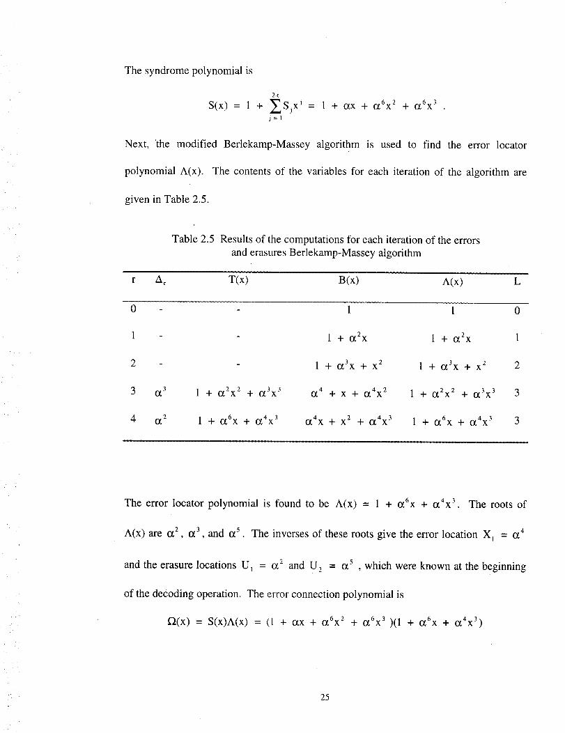
The syndrome polynomial is
2.t
S(x) = 1 + y__gjx j = 1 + o_x + O_6X2 de O_,6X 3
j=l
Next, 'the modified Berlekamp-Massey algorithm is used to find the error locator
polynomial A(x). The contents of the variables for each iteration of the algorithm are
given in Table 2.5.
Table 2.5 Results of the computations for each iteration of the errors
and erasures Berlekamp-Massey algorithm
r zX_ T(x) B(x) A(x) L
0 - 1 1 0
1 - 1 + _x2x I + _2x 1
2 - 1 + c_3x + x 2 1 + ff3x + x 2 2
3 a¢3 1 "at" O_2X 2 de 1_3X3 O_ 4 + X de O_4X 2 1 de O_2X 2 + 1_3X3 3
4 _2 1 + O_6X "t- (_4X3 [_4X 4" X 2 de _4X3 1 de O_6X de 1_4X3 3
• i
The error locator polynomial is found to be A(x) = 1 + _6X de _4X3. The roots of
A(x) are o_2 , c_3 , and ot5 . The inverses of these roots give the error location X I = 1_4
and the erasure locations U l -- c_2 and U 2 = _5 , which were known at the beginning
of the decoding operation. The error connection polynomial is
_(x) = S(x)A(x) = (1 + aCx + O_6X2 de 1_6X3 )(1 de (_6X de 0_4X 3 )
25
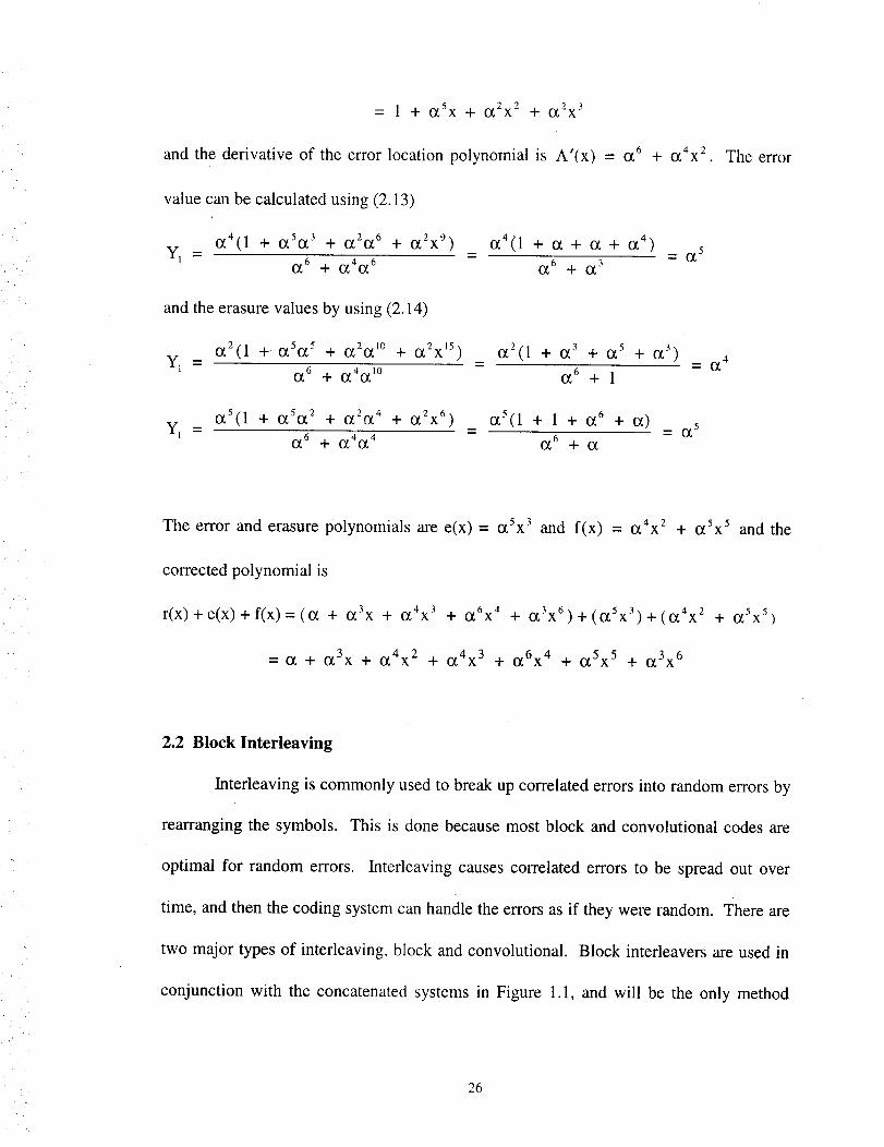
= 1 -[" (_,5X + (22X2 "[- (3_2X3
and the derivative of the error location polynomial is A'(x) = c_6 + 1_4x2.
value can be calculated using (2.13)
(24(1 + (25(23 + (22(26 ._ (22X9) (24(1 --I- (2 q- (2 -4- (_4)
Y1 = = = (25(26 .at. (24(26 (26 ,4. (23
and the erasure values by using (2.14)
(22(1 + (25(25 + (22(210 ..{_ (22X15) (22(1 + (23 '4-(25 + (23) (24Yl = = =(26 .4. (24(210 (26 "l- l
The error
The error and erasure polynomials are e(x) = (25x3 and f(x) = (24x2 at- (25x5 and the
corrected polynomial is
r(x) +e(x)+f(x)= ((2 + (23X "F (24X3 q" (26X4 q- (25X5)
= (2 + (X3X + (24X2 + (24X3
at-(23X6)-I-((25X3)--F((24X2
+ (26X4 + (25X5 + (23X6
2.2 Block Interleaving
Interleaving is commonly used to break up correlated errors into random errors by
rearranging the symbols. This is done because most block and convolutional codes are
optimal for random errors. Interleaving causes correlated errors to be spread out over
time, and then the coding system can handle the errors as if they were random. There are
two major types of interleaving, block and convolutional. Block interleavers are used in
conjunction with the concatenated systems in Figure 1.1, and will be the only method
26
discussed here. Because the interleaver is to be used in conjunction with the symbol
based Reed Solomon encoder and decoder, the interleaving will be done on a symbol
level, rather than on a bit level. Block interleavers can be implemented using an MxN
matrix. The symbols are fed into the matrix by column, and fed out by rows. At the
deinterleaving stage, the symbols are fed into the matrix by row, and output by column.
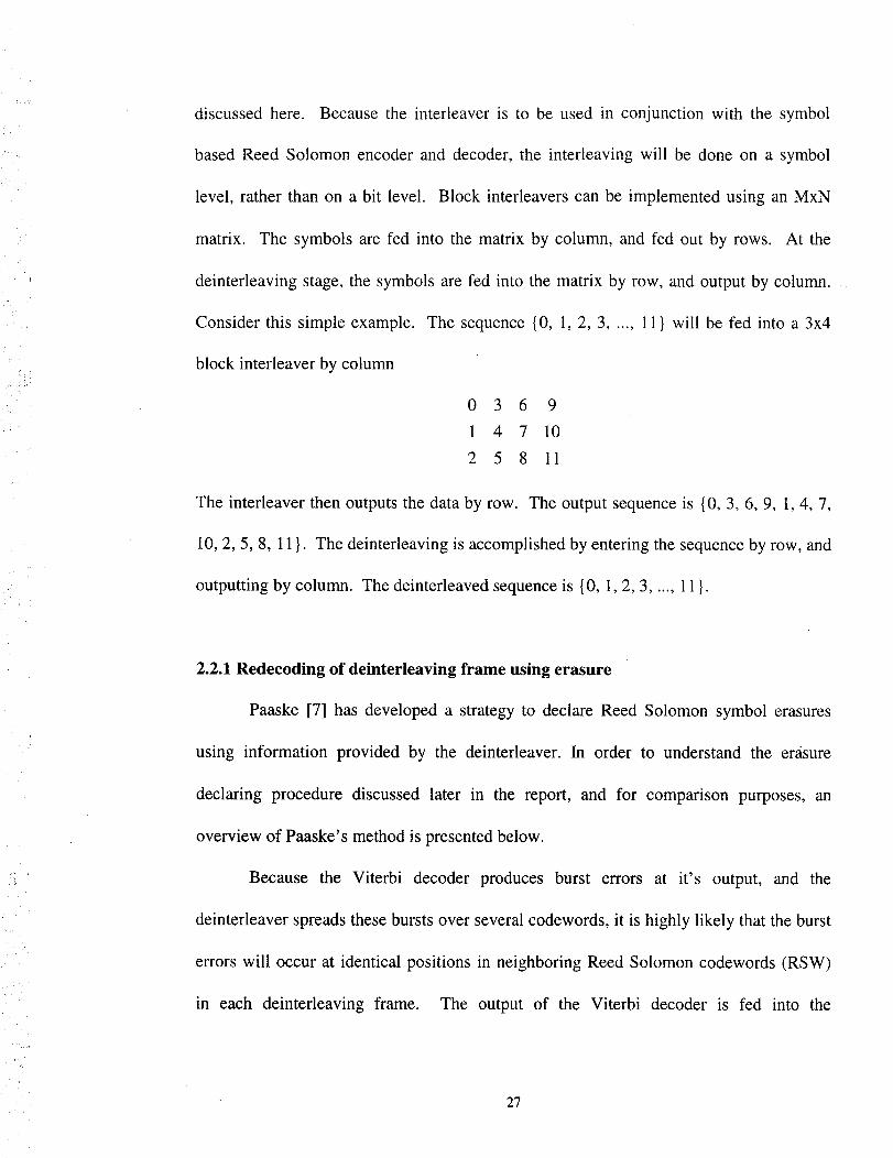
Consider this simple example. The sequence {0, 1, 2, 3 ..... 11} will be fed into a 3x4
block interleaver by column
0 3 6 9
1 4 7 10
2 5 8 11
The interleaver then outputs the data by row. The output sequence is {0, 3, 6, 9, 1, 4, 7,
10, 2, 5, 8, 11 }. The deinterleaving is accomplished by entering the sequence by row, and
outputting by column. The deinterleaved sequence is {0, 1, 2, 3 ..... 1 1 }.
2.2.1 Redecoding of deinterleaving frame using erasure
Paaske [7] has developed a strategy to declare Reed Solomon symbol erasures
using information provided by the deinterleaver. In order to understand the erasure
declaring procedure discussed later in the report, and for comparison purposes, an
overview of Paaske's method is presented below.
Because the Viterbi decoder produces burst errors at it's output, and the
deinterleaver spreads these bursts over several codewords, it is highly likely that the burst
errors will occur at identical positions in neighboring Reed Solomon codewords (RSW)
in each deinterleaving frame. The output of the Viterbi decoder is fed into the
27
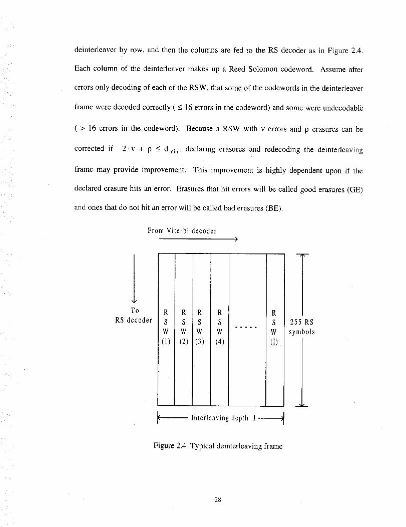
deinterleaverby row, andthen the columnsare fed to the RS decoderas in Figure 2.4.
Eachcolumn of the deinterleavermakesup a ReedSolomoncodeword. Assumeafter
errorsonly decodingof eachof theRSW, thatsomeof thecodewordsin thedeinterleaver
frameweredecodedcorrectly( _<16errorsin thecodeword)andsomewereundecodable
( > 16 errors in the codeword). Becausea RSW with v errorsand p erasurescanbe
correctedif 2. v -I- p _< dmin, declaring erasures and redecoding the deinterleaving
frame may provide improvement. This improvement is highly dependent upon if the
declared erasure hits an error. Erasures that hit errors will be called good erasures (GE)
and ones that do not hit an error will be called bad erasures (BE).
From Viterbi decoder)
To
RS decoderR
S
W
(1)
R
S
W
(2)
I
R R R
S S S 255 RSa . o _ t
W W W symbols
(3) (4) (I)
Interleaving depth I
i
Figure 2.4 Typical deinterleaving flame
28
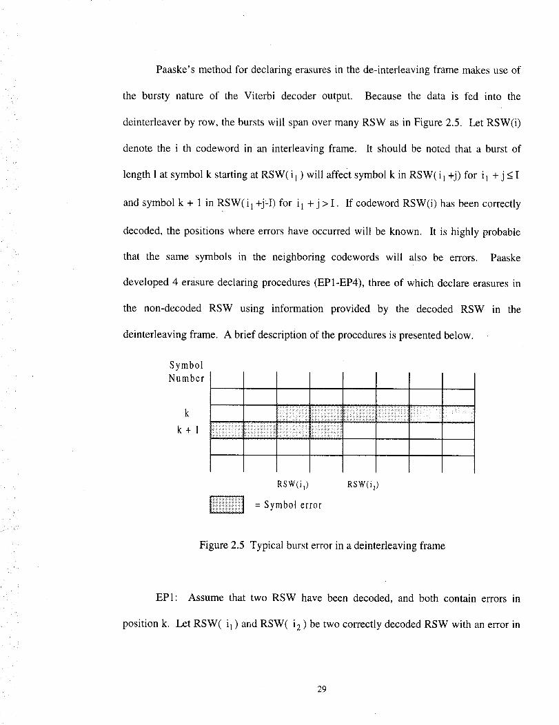
Paaske'smethodfor declaringerasuresin thede-interleavingflamemakesuseof
the bursty nature of the Viterbi decoderoutput. Becausethe data is fed into the
deinterleaverby row, theburstswil ! spanovermanyRSW asin Figure2.5. Let RSW(i)
denotethe i th codewordin an interleavingframe. It shouldbe noted that a burst of
length1at symbolk startingat RSW(i I ) will affect symbolk in RSW(i I +j) for i1+ j < I
and symbol k + 1 in RSW(i 1+j-I) for i 1 + j > I. If codeword RSW(i) has been correctly
decoded, the positions where errors have occurred will be known. It is highly probable
that the same symbols in the neighboring codewords will also be errors. Paaske
developed 4 erasure declaring procedures (EP1-EP4), three of which declare erasures in
the non-decoded RSW using information provided by the decoded RSW in the
deinterleaving frame. A brief description of the procedures is presented below.
Symbol
Number I
k
k+l
I I I
:::::::::::::::::::::::::::::::::::::::::::::::::::::::::::::::::::::::::::::::::::::::: :77 r_
ilii!i_!_•_!_i_!_iiiii!;_!iii_iiiiiii_!_i_iii_i_i_iiii_!iiiiiii_i!i_ii_iiiii_iiiiiii_iii_iiiiii_ii_ii_!_iiiii_iiii!iiiii_i_;i_!_!i_?__ill_:I! _5::7.>:•.>• :H +...•+•+H•.... •••.....•H:•• : •••.•••••••• T..• ••••H..•.H•••.•.•..•" _ ............... _'_ _::_:: ::"
:':+::+:+:+ "'••+:_:+:+:::+.+:+:+:+:':" :::>:':F::F• :+:4• :+:'<•:':':+: + :+:•':+:+:+ >> +S+: •'+:+:+:+•':':+:+:+:': ':+:: >: • + "• +:+• :'X':+•+: : :':':':':+:':+:':::::::::::::::::::::::::::::::::::::::::::::::::::::::::::::::::::::::: ::: :::': ::': _'i:_:: ::::::::::::::::::::::
_''" " .......... " ............... _ ................ _:':llllll'flllllfH'
RSW(i I)
= Symbol error
RSW(i 2)
Figure 2.5 Typical burst error in a deinterleaving frame
EPl: Assume that two RSW have been decoded, and both contain errors in
position k. Let RSW( i 1) and RSW( i 2 ) be two correctly decoded RSW with an error in
29
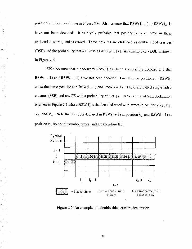
position k in both as shown in Figure 2.6. Also assume that RSW(i 1+1) to RSW(i2-1 )
have not been decoded. It is highly probable that position k is an error in these
undecoded words, and is erased. These •erasures are classified as double sided erasures
(DSE) and the probability that a DSE is a GE is 0.96 [7]. An example of a DSE is shown
in Figure 2.6.
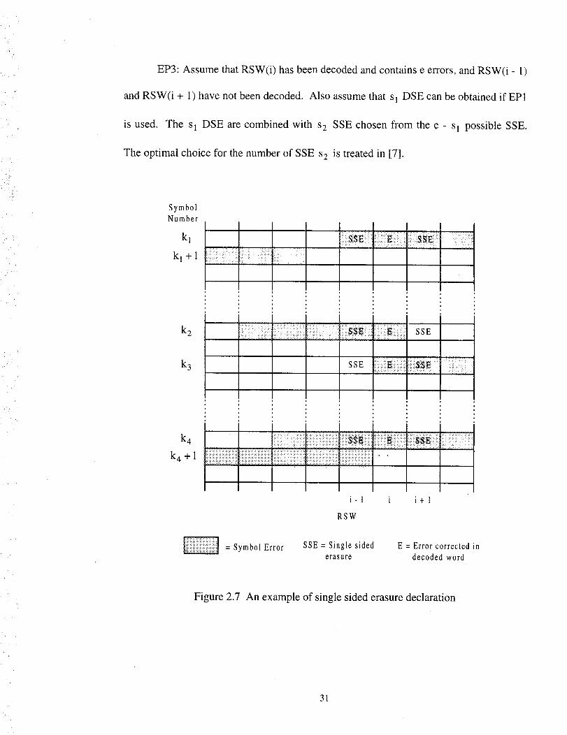
EP2: Assume that a codeword RSW(i) has been successfully decoded and that
RSW(i - I) and RSW(i + 1) have not been decoded. For all error positions in RSW(i)
erase the same positions in RSW(i - 1) and RSW(i + 1). These are called single sided
erasures (SSE) and are GE with a probability of 0.60 [7]. An example of SSE declaration
is given in Figure 2.7 where RSW(i) is the decoded word with errors in positions k I , k 2 ,
k 3 , and k 4 . Note that the SSE declared in RSW(i + 1) at position k 2 and RSW(i - 1) at
position k 3 do not hit symbol errors, and are therefore BE.
Symbol
Number
k-1
k
k+l
i_ i1 +1 i2 -1 i2
RSW
= Symbol Error DSE = Double sided E = Error corrected it,,erasure decoded word
Figure 2.6 An example of a double sided erasure declaration
3o
:i_i_
EP3: Assume that RSW(i) has been decoded and contains e errors, and RSW(i - 1)
and RSW(i + 1) have not been decoded. Also assume that s I DSE can be obtained if EP1
is used. The s 1 DSE are combined with s 2 SSE chosen from the e - s I possible SSE.
The optimal choice for the number of SSE s 2 is treated in [7].
Symbol
Number
kl
kl+l iii_i!ii!i!ii_i!:•_ii:liiii!__ _iiiiiii_:_:_i_iiii_i!ii
k 2
k 3
,_ SSE
SSE i ii i:Eiii:_ i i::i:ii$_E :"• +:: ::::::: ': :::_: :) • :il;_,i:i
k 4
k4+l
:::::::::::_::::::: :::: ::::: :: ::4::.:.:::: ::.:::::: :.:1-:::: ::!!!!! :.::: : : :_.:: : :: :::_:::_::::::::: :::::
+::.:+:..:+:.:.:.:+:.:.: ::::::::::::::::::::::::::::::::::: ::::5::: :::_::::::: .:: : :. :.:::. _: ::::::::::::::::::::::::
::::::::::::::::::::::::::: :: ':':':':':':"'"'"'""'"'"'" "" '"" !'!'i'i "':'; ":':':':':':':': :;:_;:;:;:;:; ;: ::;:;:;:;:;:;:;;;:;:;:;:';:'"
i-1
RSW
i i+l
= Symbol Error SSE = Single sided E = Error corrected
erasure decoded word
Figure 2.7 An example of single sided erasure declaration
in
31
i ¸
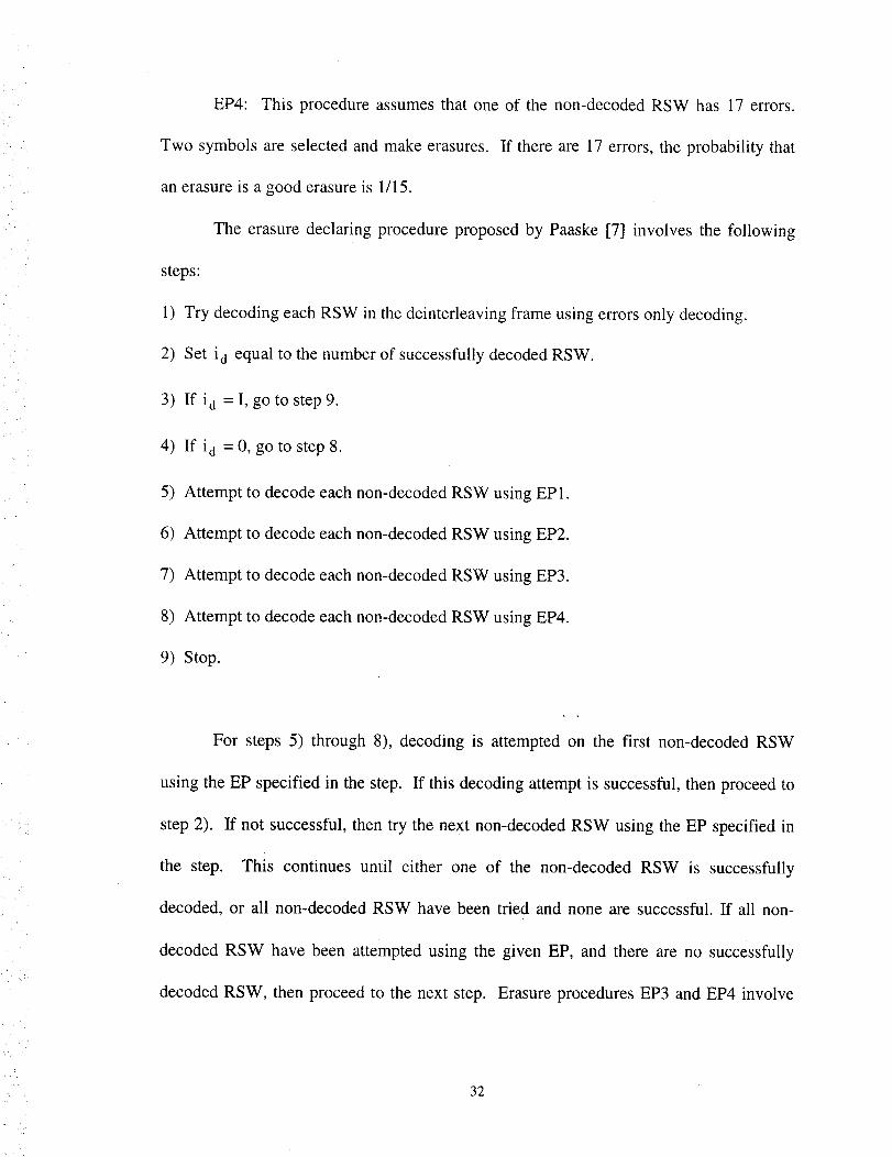
EP4: This procedure assumes that one of the non-decoded RSW has 17 errors.
Two symbols are selected and make erasures. If there are 17 errors, the probability that
an erasure is a good erasure is 1/15.
The erasure declaring procedure proposed by Paaske [7] involves the following
steps:
1) Try decoding each RSW in the deinterleaving frame using errors only decoding.
2) Set i d equal to the number of successfully decoded RSW.
3) If i d = I, go to step 9.
4) If i d = 0, go to step 8.
5) Attempt to decode each non-decoded RSW using EP1.
6) Attempt to decode each non-decoded RSW using EP2.
7) Attempt to decode each non-decoded RSW using EP3.
8) Attempt to decode each non-decoded RSW using EP4.
9) Stop.
For steps 5) through 8), decoding is attempted on the first non-decoded RSW
using the EP specified in the step. If this decoding attempt is successful, then proceed to
step 2). If not successful, then try the next non-decoded RSW using the EP specified in
the step. This continues until either one of the non-decoded RSW is successfully
decoded, or all non-decoded RSW have been tried and none are successful. If all non-
decoded RSW have been attempted using the given EP, and there are no successfully
decoded RSW, then proceed to the next step. Erasure procedures EP3 and EP4 involve
32
selectingerasuresin a systematicway. This step is repeatedon eachcodeworduntil
either a successfuldecodingof thecodeword,or a maximumnumberof trials Tma x has
been attempted. In the simulations conducted by Paaske, Trnax = 500 trials.
2.3 Convolutional codes
Convolutional codes are fundamentally different than block codes. Block codes
divide the information sequence into segments of length k, and map these k bits onto a
codeword of length n. Convolutional codes on the other hand convert the entire data
stream into one code word, regardless of the length of the information sequence. A (n, k,
m) convolutional encoder has k inputs and n outputs, where k < n and both k and n are
small integers. The memory order m should be made large in order to achieve a high
degree of error correcting capability [6].
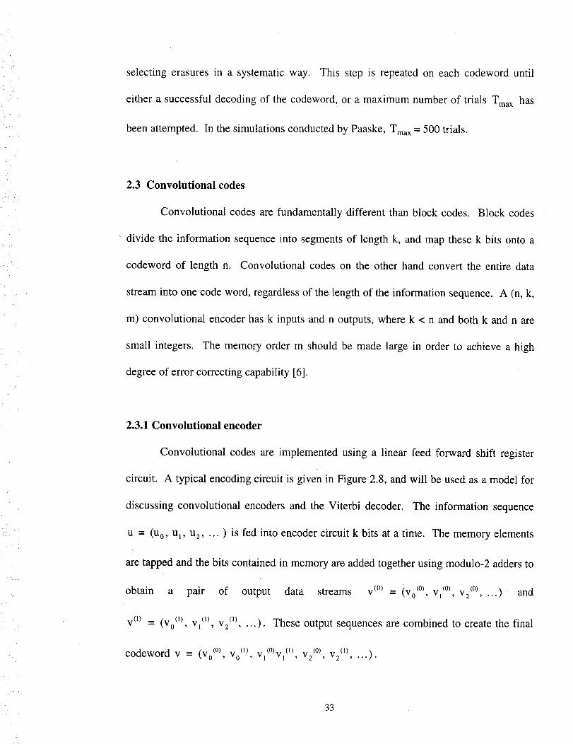
2.3.1 Convolutional encoder
Convolutional codes are implemented using a linear feed forward shift register
circuit. A typical encoding circuit is given in Figure 2.8, and will be used as a model for
discussing convolutional encoders and the Viterbi decoder. The information sequence
u•= (u 0, u_, u 2 .... ) is fed into encoder circuit k bits at a time. The memory elements
are tapped and the bits contained in memory are added together using modulo-2 adders to
obtain a pair of output
V (l) = (Vo (1), VL (l), V2 (1) .... ).
codeword v = (Vo (°), Vo(_), Vl(O)Vl (1), V2 (0), V2(1)
data streams v (°) = (Vo(°>, v_(°), v2 (°).... ) and
These output sequences are combined to create the final
, ...)*
33
:i: ,:
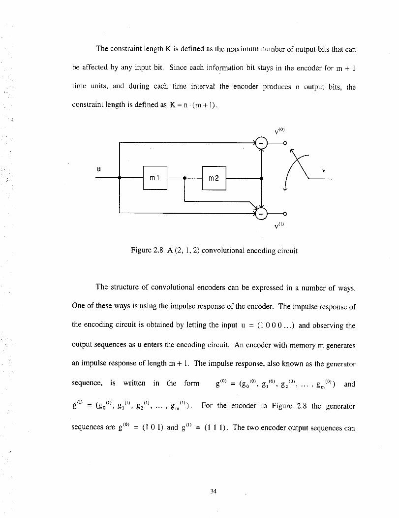
The constraint length K is defined as the maximum number of output bits that can
be affected by any input bit. Since each information bit stays in the encoder for m + 1
time units, and during each time interval the encoder produces n output bits, the
constraint length is defined as K = n. (m + 1).
u
ml T m2
V (o)
7---o
L:V (l)
Figure 2.8 A (2, 1, 2) convolutional encoding circuit
The structure of convolutional encoders can be expressed in a number of ways.
One of these ways is using the impulse response of the encoder. The impulse response of
the encoding circuit is obtained by letting the input u - (1 0 0 0...) and observing the
output sequences as u enters the encoding circuit. An encoder with memory m generates
an impulse response of length m + 1. The impulse response, also known as the generator
sequence, is written in the form g(O) = (go(O), g(O), g2(O) ..... g (o)) andm
g(_) = (go (a), g_(_), g2 (_)..... gm(1)). For the encoder in Figure 2.8 the generator
sequences are g(O) = (1 0 1) and g(_) = (1 1 1). The two encoder output sequences can
34
be thought of as a linear convolution of the information sequence with the impulse
response. The encoding equations can be written as
v (°_ = u * g(0_ (2.15a)
v (l_ = u* g(Z_ (2.15b)
where * denotes discrete convolution using modulo-2 operations. The output at time t - '_
can be written as
m
vx(J) = Zuz-i. gi j
i=0
=U_ .go (j) + Ux_ 1 .gl (j) + Ux_ 2 .g2 (j) + ... +Uz_ m .gin (j). (2.16)
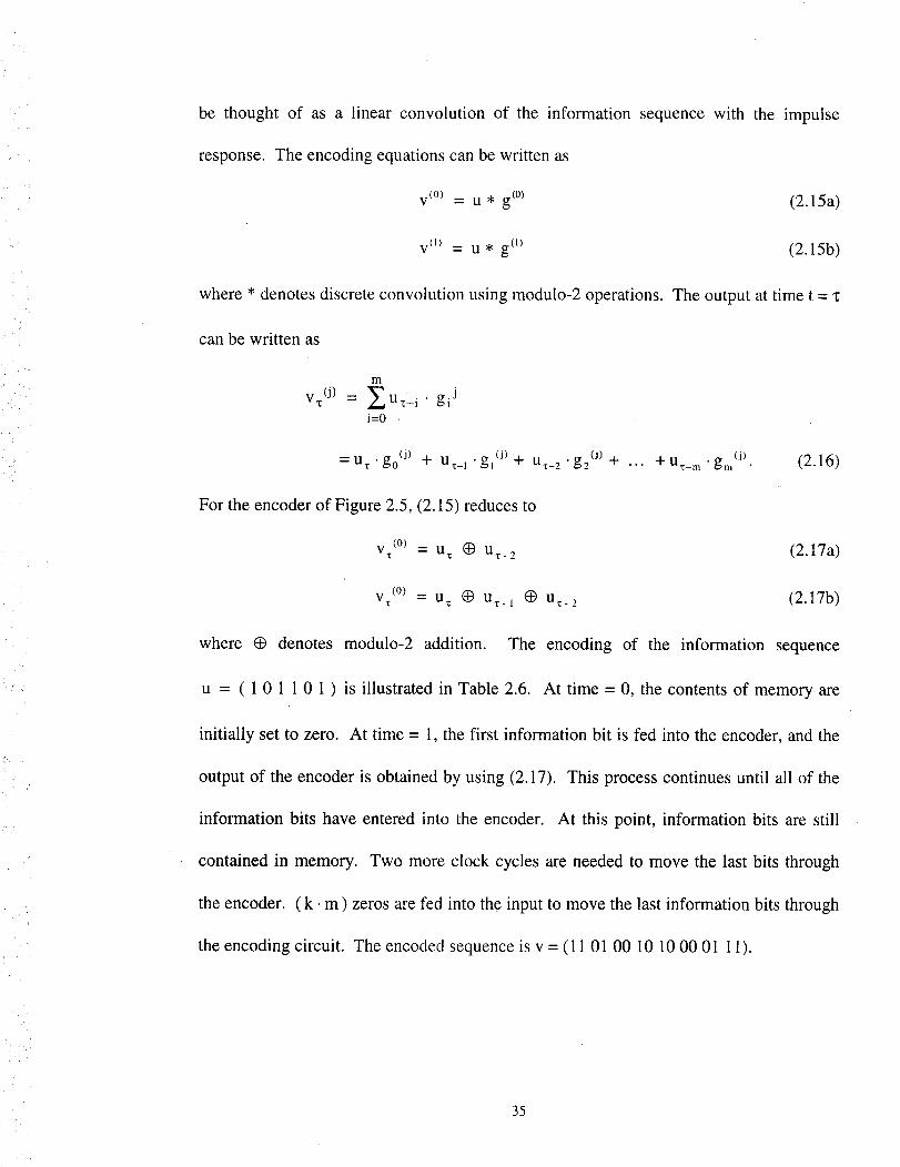
For the encoder of Figure 2.5, (2.15) reduces to
v_ (°) = u_ _ u_.2 (2.17a)
v,_(0) -- u,_ (_ u,_. 1 (_ u,l:.2 (2.17b)
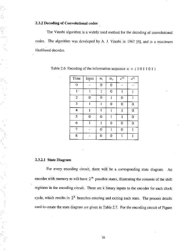
where _ denotes modulo-2 addition. The encoding of the information sequence
u = ( 1 0 1 1 0 1 ) is illustrated in Table 2.6. At time = 0, the contents of memory are
initially set to zero. At time = 1, the first information bit is fed into the encoder, and the
output of the encoder is obtained by using (2.17). This process continues until all of the
information bits have entered into the encoder. At this point, information bits are still
contained in memory. Two more clock cycles are needed to move the last bits through
the encoder. (k. m) zeros are fed into the input to move the last information bits through
the encoding circuit. The encoded sequence is v = (11 01 00 10 10 00 01 11).
35
2.3.2 Decoding of Convolutional codes
The Viterbi algorithm is a widely used method for the decoding of convolutional
codes. The algorithm was developed by A. J. Viterbi in 1967 [6], and is a maximum
likelihood decoder.
Table 2.6 Encoding of the information sequence u = ( 1 0 1 1 0 1 )
Time I InputI
0
1 1
2 0
3 1
4 1
5 0
6 1
7
8
ml m2 v (°) v(l)
0 0
1 0 1 1
0 1 0 1
1 0 0 0
1 1 1 0
0 1 1 0
1 0 0 0
0 1 0 1
0 0 1 1
2.3.2.1 State Diagram
For every encoding circuit, there will be a corresponding state diagram. An
encoder with memory m will have 2 m possible states, illustrating the contents of the shift
registers in the encoding circuit. There are k binary inputs to the encoder for each clock
cycle, which results in 2 k branches entering and exiting each state. The process details
used to create the state diagram are given in Table 2.7. For the encoding circuit of Figure
36
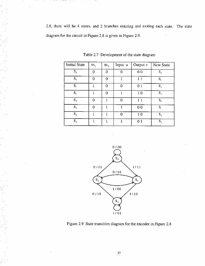
2.8, there will be 4 states, and 2 branches entering and exiting each state.
diagram for the circuit in Figure 2.8 is given in Figure 2.9.
The state
Table 2.7 Development of the state diagram
Initial State m_ m 2
S. 0 0
So 0 0
Sl 1 0
Sl 1 0
$2 0 1
$2 0 1
$3 1 1
$3 1 1
Input u Output v New State
0 0 0 S,,
1 1 1 Si
0 0 1 $2
1 I 0 $3
0 1 1 S,,
1 0 0 Sl
0 1 0 $2
1 0 1 $3
0/00
0/10 NN@ 1/10
1/01
Figure 2.9 State transition diagram for the encoder in Figure 2.8
37
-_ i_
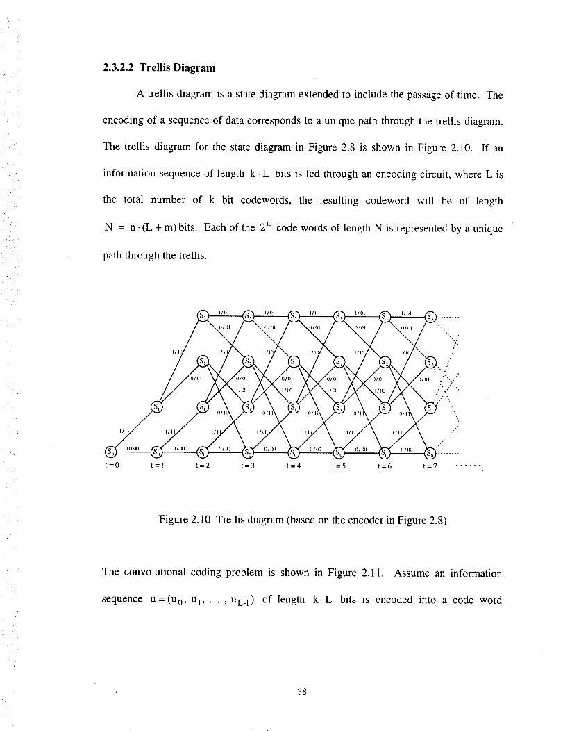
2.3.2.2 Trellis Diagram
A trellis diagram is a state diagram extended to include the passage of time. The
encoding of a sequence of data corresponds to a unique path through the trellis diagram.
The trellis diagram for the state diagram in Figure 2.8 is shown in Figure 2.10. If an
information sequence of length k. L bits is fed through an encoding circuit, where L is
the total number of k bit codewords, the resulting codeword will be of length
N = n. (L + m) bits. Each of the 2 _ Code words of length N is represented by a unique
path through the trellis.
I/l( i';'
{)/(}1 ', ,' ",, .'"
t=O t=l t=2 t=3 t=4 t=5 t=6 t=7 ......
Figure 2.10 Trellis diagram (based on the encoder in Figure 2.8)
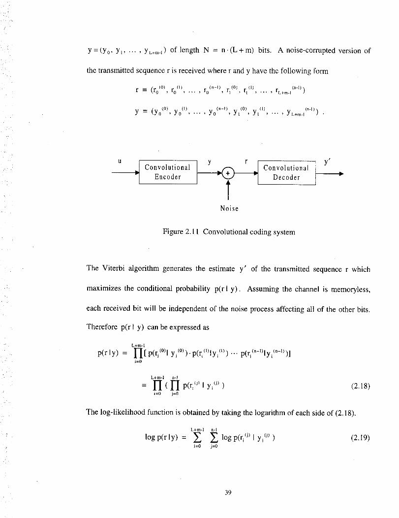
The convolutional coding problem is shown in Figure 2.11. Assume an information
sequence u =(u 0, u 1..... UL_l) of length k.L bits is encoded into a code word
38
i ¸
Y = (Yo, Y_..... YL+m-I) of length N = n. (L + m) bits. A noise-corrupted version of
the transmitted sequence r is received where r and y have the following form
r = (ro (°), ro¢1) ro(n-t), rl(o) rl(1) (n-I), ... , , , ... , rL+m. I )
y = (yo(O), yo(_) ..... y0(n-t), y(0_, y(_ ..... YL+m. (n-_) .
U y',j Convolutional ]
" Encoder
TNoise
Convolutional
Decoder
Figure 2.11 Convolutional coding system
The Viterbi algorithm generates the estimate y' of the transmitted sequence r which
maximizes the conditional probability p(rl y). Assuming the channel is memoryless,
each received bit will be independent of the noise process affecting all of the other bits.
Therefore p(rl y) can be expressed as
L+m-1
p(r ly) = l-I[ p(ri (°)1 Yi (°))" P(ri°)lyi 0)) "'" P(ri(n-l)lyi(n-l_)]i=O
L+m-I n-]
= 1-I ( 1-I P(r_(J) I Y_(j_) (2.18)i=o j=o
The log-likelihood function is obtained by taking the logarithm of each side of (2.18).
L+m-I n-I
log p(r ly) = ,_, _, log P(ri (j) I yi (j))i=O j=O
(2.19)
39

(
/
This is done because it is, in general, easier to implement summations rather than
multiplication in hardware. The log likelihood function, log p(r ly), is called the Path
Metric associated with the path y and is denoted M(rl y). The terms log p(r, _) ly_ _)) are
called Bit Metrics
M(r_ °) ly_ °)) = log p(q0)ly0)) (2.20)
In the hardware implementation of the Viterbi decoder, it is more convenient to use
positive integers for the metric values rather than the actual bit metrics. This can be
accomplished by using
M(ri(J) lYi(J)) = a.[logp(ri0)lYi (,j)) + b] (2.21)
where a and b are chosen to obtain small, positive integer values for the metrics which
can be implemented easier in hardware.• The path metric for a codeword y is then
calculated as
L+m-I n-I
M(rly) = _ _LM(r_)ly_°)). (2.22)i=o j=o
The k th branch metric for a codeword y is defined as the sum of the bit metrics
n-I
M(r k I Yk) = ZM(rk (j) l Yk(3)) • (2.23)j=0
The k th partial metric for a path is obtained by summing all of the branch metrics for the
first k branches the path follows.
k-I
Mk(rl y) = .__M(r i lYi)j=O
(2.24)
k-I n-I
_ M(ri 0, lyi(J)).i=O j=O
(2.25)
40
The Viterbi Algorithm finds the path through the trellis with the largestpath metric,
which is the maximum likelihood estimatey' of the receivedword r. At eachtime
interval the algorithm, computesthe partial metrics enteringeach state. The largest
metric is chosenasthesurvivingpathateachstate,andall otherpathsenteringthat state
arediscarded.This processis continueduntil the endof thetrellis is reached.The final
survivingpathis themaximumlikelihoodestimatey of thecodeword.
2.3.2.3 The Viterbi Algorithm [6]
1. At time t = m, compute the partial metric for the single path entering each
state. Store the value of this metric at each state.
2. Increase t by 1. Compute the partial metric for the path entering each state.
This will be equal to the branch metric entering the state plus the surviving metric from
the previous state. Out of the 2 k paths entering each state, the path with the largest metric
is chosen and the remaining paths are discarded. The metric of the surviving path is
stored at each state.
3. Ift<L+m, repeat step 2. If not, stop. At timet=L+m, all paths have
returned to the all zero state. There will be only one path remaining, and this path is the
maximum likelihood estimate y'.
2.3.2.4 Hard Decision Decoding
In hard decision decoding, the receiver determines whether a zero or one was
transmitted. These zeros and ones are the input to the Viterbi decoder. If the channel is
41
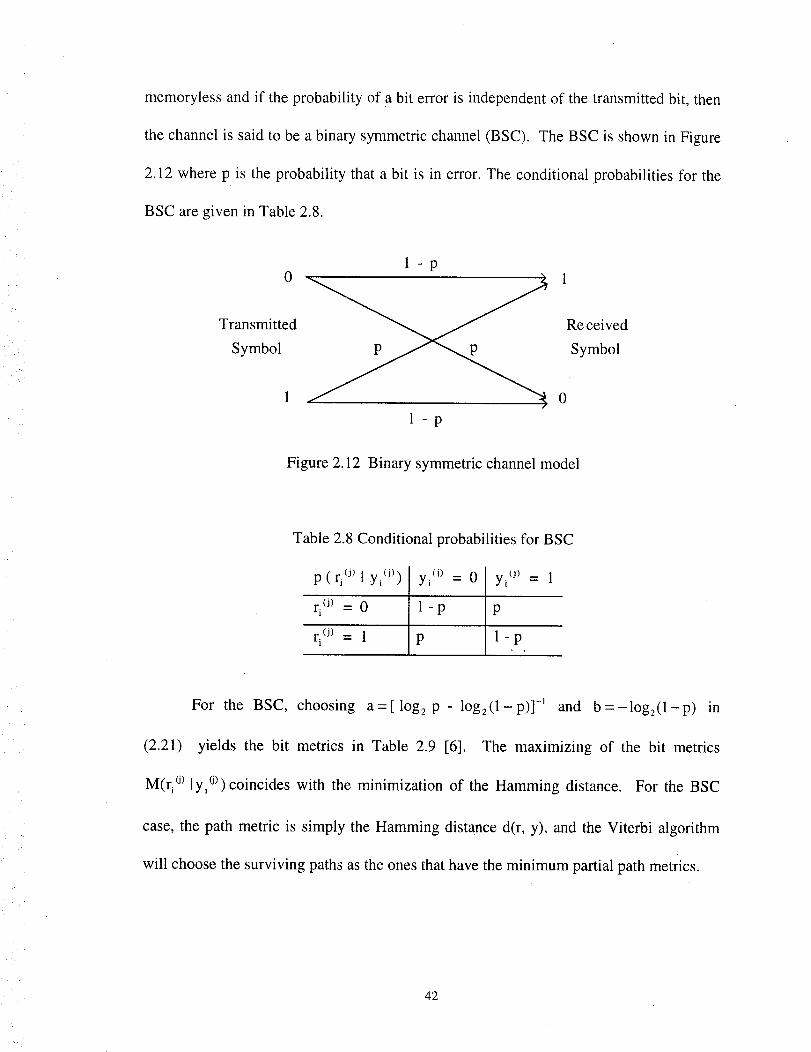
memorylessand if theprobabilityof a bit error is independentof thetransmittedbit, then
thechannelis saidto beabinarysymmetricchannel(BSC). TheBSC is shownin Figure
2.12wherep is theprobability that abit is in error.Theconditionalprobabilitiesfor the
BSC aregiven in Table2.8.
1-p0 1
Transmitted Received
Symbol Symbol
1 01 - p
Figure2.12 Binarysymmetricchannelmodel
Table2.8Conditionalprobabilitiesfor BSC
p ( ri ° I yi (j))
ri ° = 0
ri ° = 1 p
yi (j) = 0 [
1-p [ p1-p
yi (j) = 1
For the BSC, choosing a=[log 2 p - log2(1-p)] -1 and b=-log2(1-p) in
(2.21) yields the bit metrics in Table 2.9 [6]. The maximizing of the bit metrics
M(r_ °) lYi°))coincides with the minimization of the Hamming distance. For the BSC
case, the path metric is simply the Hamming distance d(r, y), and the Viterbi algorithm
will choose the surviving paths as the ones that have the minimum partial path metrics.
42
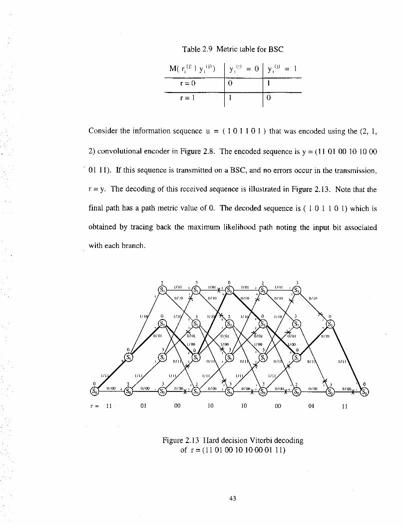
" Table 2.9 Metric table for BSC
M( ri(J) l yi (i)) (J) 0Yi - yi (j) = 1
r=0 0 1
r=l 1 0
Consider the information sequence u = ( 1 0 1 1 0 1 ) that was encoded using the (2, 1,
2) convolutional encoder in Figure 2.8. The encoded sequence is y = (11 01 00 10 10 00
01 11). If this sequence is transmitted on a BSC, and no errors occur in the transmission,
r = y. The decoding of this received sequence is illustrated in Figure 2.13. Note that the
final path has a path metric value of 0. The decoded sequence is ( 1 0 1 1 0 1) which is
obtained by tracing back the maximum likelihood path noting the input bit associated
with each branch.
2 3 0 2 3
o o
r = 11 01 00 10 I0 00 O1 11
Figure 2.13 Hard decision Viterbi decoding
of r = (l l 01001010 00 01 11)
43
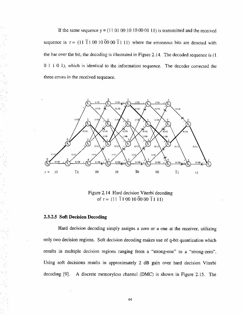
If the same sequence y = (11 01 00 10 10 00 01 1 l) is transmitted and the received
sequence is r = (11 T1 00 10 O0 00 ]-1 11) where the erroneous bits are denoted with
the bar over the bit, the decoding is illustrated in Figure 2.14. The decoded sequence is ( 1
0 1 1 0 1), which is identical to the information sequence. The decoder corrected the
three errors in the received sequence.
]i:
1 2 1 I 2
S It /01. '53 I/Ol 2531/Ol 153 1/01 i_
0 2
r = 11 TI O0 10 O0 O0 TI 11
Figure 2.14 Hard decision Viterbi decoding
of r= (l l ll 0010 00 00 T1 11)
2.3.2.5 Soft Decision Decoding
Hard decision decoding simply assigns a zero or a one at the receiver, utilizing
only two decision regions. Soft decision decoding makes use of q-bit quantization which
results in multiple decision regions ranging from a "strong-one" to a "strong-zero".
Using soft decisions results in approximately 2 dB gain over hard decision Viterbi
decoding [9]. A discrete memoryless channel (DMC) is shown in Figure 2.15. The
44
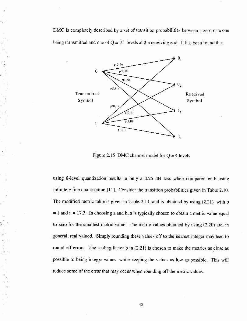
DMC is completely described by a set of transition probabilities between a zero or a one
being transmitted and one of Q = 2 q levels at the receiving end. It has been found that
0
o,
p( ,I ) 02
T,.ansm,tte , eceivedSymbol Symbol
P(IOI) _ _.
11
Figure 2.15 DMC channel model for Q = 4 levels
using 8-level quantization results in only a 0.25 dB loss when compared with using
infinitely fine quantization [ 11]. Consider the transition probabilities given in Table 2.10.
The modified metric table is given in Table 2.11, and is obtained by using (2.21) with b
= 1 and a = 17.3. In choosing a and b, a is typically chosen to obtain a metric value equal
to zero for the smallest metric value. The metric values obtained by using (2.20) are, in
general, real valued. Simply rounding these values off to the nearest integer may lead to
round off errors. The scaling factor b in (2.21) is chosen to make the metrics as close as
possible to being integer values, while keeping the values as low as possible. This will
reduce some of the error that may occur when rounding off the metric values.
45
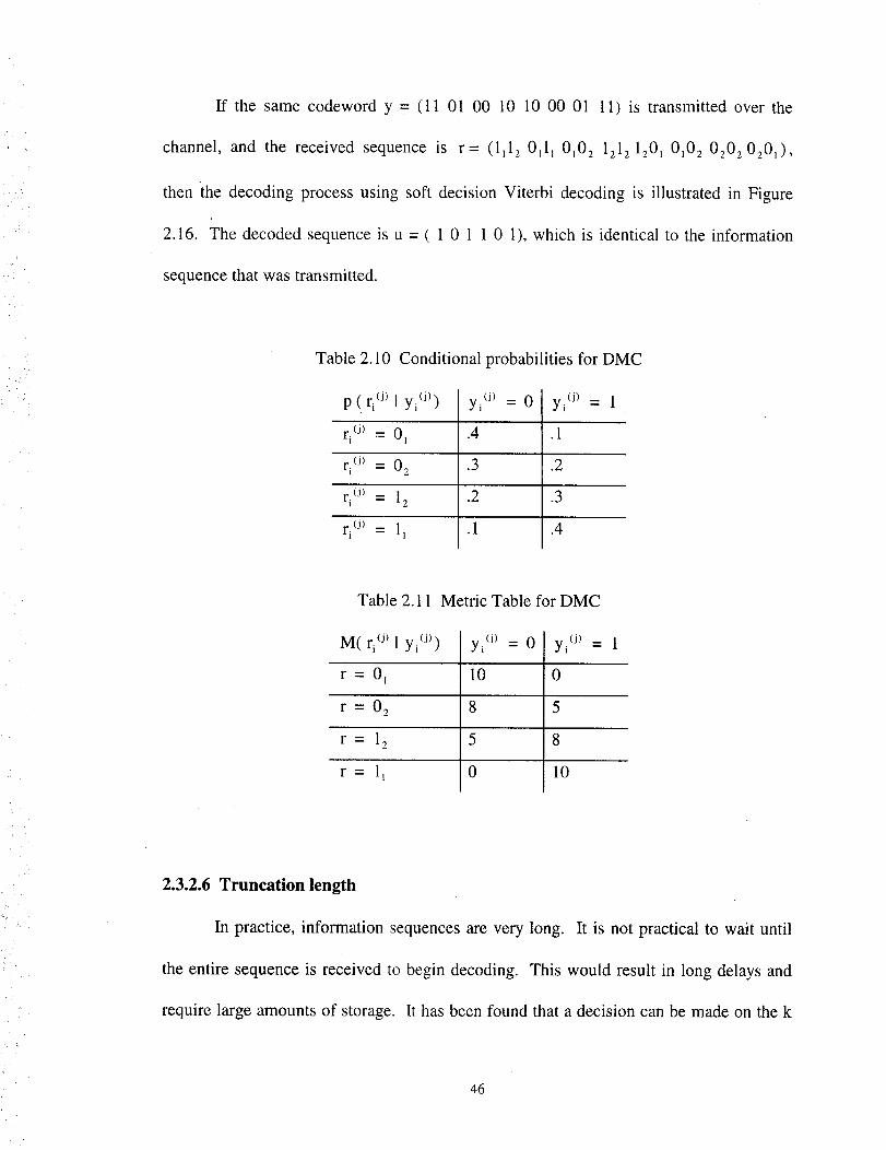
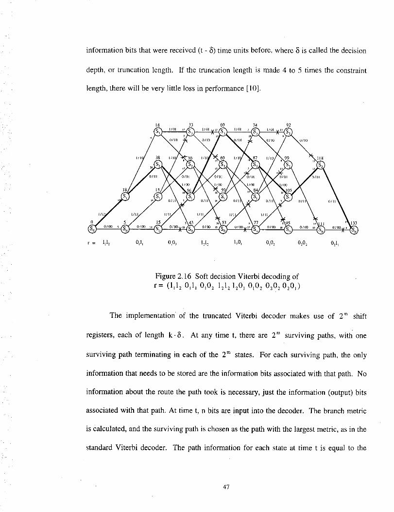
If the same codeword y = (11 01 00 10 10 00 01 11) is transmitted over the
channel, and the received sequence is r= (lll 2 0111 0t02 1212 1201 010 2 0202 0201) ,
then the decoding process using soft decision Viterbi decoding is illustrated in Figure
2.16. The decoded sequence is u = ( 1 0 1 1 0 1), which is identical to the information
sequence that was transmitted.
Table 2.10 Conditional probabilities for DMC
P ( ri (j) [ y_(J)) yi (j) = 0 yi (j) = 1
ri (j) = 01 .4 .1
ri (j) = 0 2 .3 .2
r_(j) = 12 .2 .3
ri O) = 11 .I .4
Table 2.11 Metric Table for DMC
M( ri(J) l yi (j))
r=O l
r=O 2
r=l 2
r=l I
yi (j) = 0 yi (j) = 1
10 0
8 5
5 8
0 10
L
i•
2.3.2.6 Truncation length
In practice, information sequences are very long. It is not practical to wait until
the entire sequence is received to begin decoding. This would result in long delays and
require large amounts of storage. It has been found that a decision can be made on the k
46
information bits that were received (t - 8) time units before, where 8 is called the decision
depth, or truncation length. If the truncation length is made 4 to 5 times the constraint
length, there will be very little loss in performance [10].
18 33 69 74 92
(I 0 / I0
0 133
r = lllz 0ill 0102 1212 120i 0102 0202 021 '
Figure 2.16 Soft decision Viterbi decoding of
r= (1112 0111 0102 1212 1201 0102 0202 0201)
The implementation of the truncated Viterbi decoder makes use of 2 m shift
registers, each of length k. 8. At any time t, there are 2 m surviving paths, witla one
surviving path terminating in each of the 2 m states. For each surviving path, the only
information that needs to be stored are the information bits associated with that path. No
information about the route the path took is necessary, just the information (output) bits
associated with that path. At time t, n bits are input into the decoder. The branch metric
is calculated, and the surviving path is chosen as the path with the largest metric, as in the
standard Viterbi decoder. The path information for each state at time t is equal to the
47
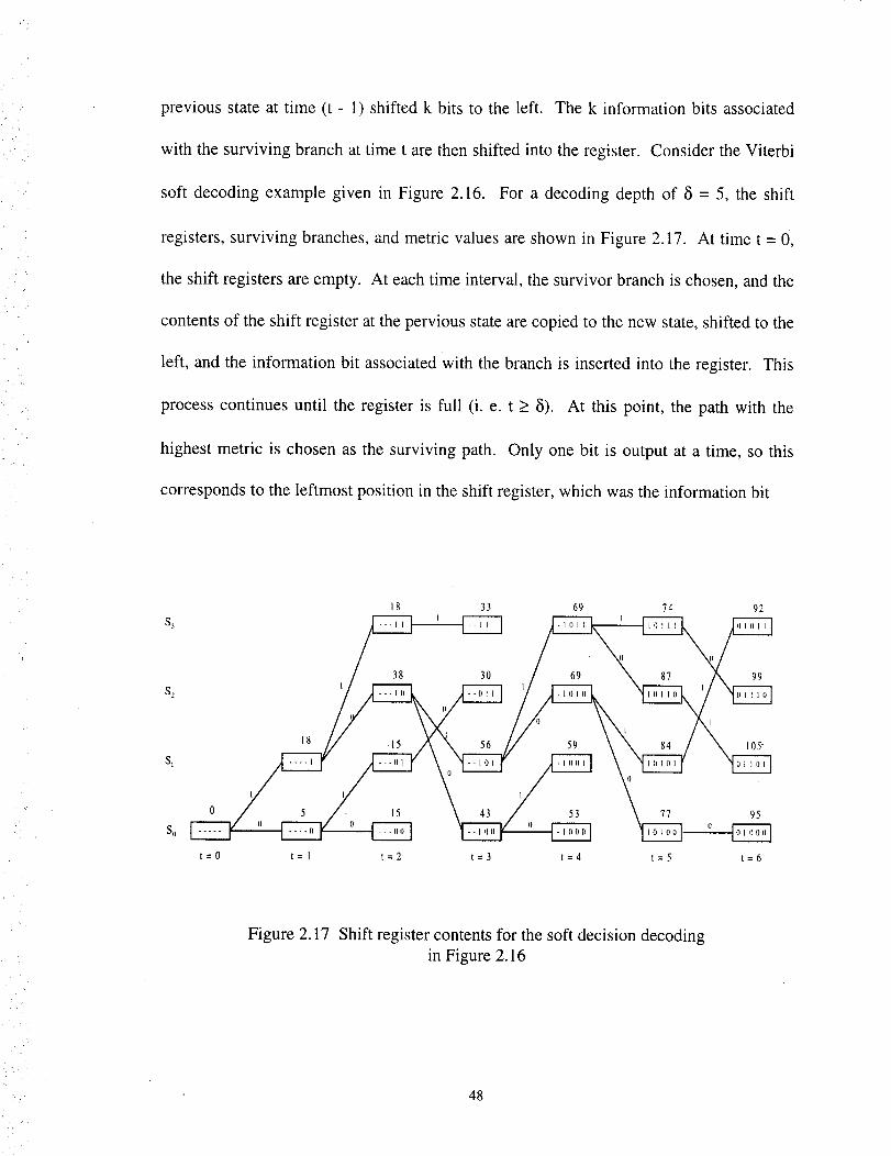
previous state at time (t - 1) shifted k bits to the left. The k information bits associated
with the surviving branch at time t are then shifted into the register. Consider the Viterbi
soft decoding example given in Figure 2.16. For a decoding depth of 5 = 5, the shift
registers, surviving branches, and metric values are shown in Figure 2.17. At time t = 0,
the shift registers are empty. At each time interval, the survivor branch is chosen, and the
contents of the shift register at the pervious state are copied to the new state, shifted to the
left, and the information bit associated with the branch is inserted into the register. This
process continues until the register is full (i. e. t > 8). At this point, the path with the
highest metric is chosen as the surviving path. Only one bit is output at a time, so this
corresponds to the leftmost position in the shift register, which was the information bit
18 33 69 74 92
0
/ / \ / \0 5 15 43 ...... 53 77 9
so _
t=O t=l t=2 t=3 t=4 t=5 t=6
Figure 2.17 Shift register contents for the soft decision decoding
in Figure 2.16
48
.: _i ¸
ili !iiiii
inserted t - 8 time units before. In Figure 2.17 at t = 5 = 5, the path with the highest
metric has a path metric of 87, and terminates in state S 2 . The leftmost bit in the shift
register is equal to 1, and is the output for this time interval. Now, since t > 8, the
decoder can take in n bits, compute the path metric and determine the surviving path for
each state. The decoder then chooses the path with the maximum metric, and outputs the
leftmost bit. At time t = 6 in Figure 2.17, the path with the highest metric has a path
metric equal to 105, and terminates in state S_. The leftmost bit in that shift register is 0,
and is the output bit. This process continues for the remainder of the decoding operation.
2.3.3 Soft Output Viterbi Algorithm
The Viterbi algorithm can be modified to give either a reliability value or a
probability that a given bit is correct. The method used to implement the Soft Output
Viterbi Algorithm (SOVA) is based upon Hagenauer and Hoeher's method [4]. For
simplicity, this discussion will only consider convolutional codes where k = 1. The
reliability of a binary random variable can be defined in terms of a log-likelihood value
Prob(u = 1)L(u) = log (2.26)
Pr ob(u = 0)
where the sign of L(u) corresponds to the hard decision (i.e. if L(u) > 0, u = 1 and if L(u)
< 0, u = 0) and the magnitude IL(u)l is the reliability of this decision. The larger the
magnitude, the greater the reliability of the decision.
49
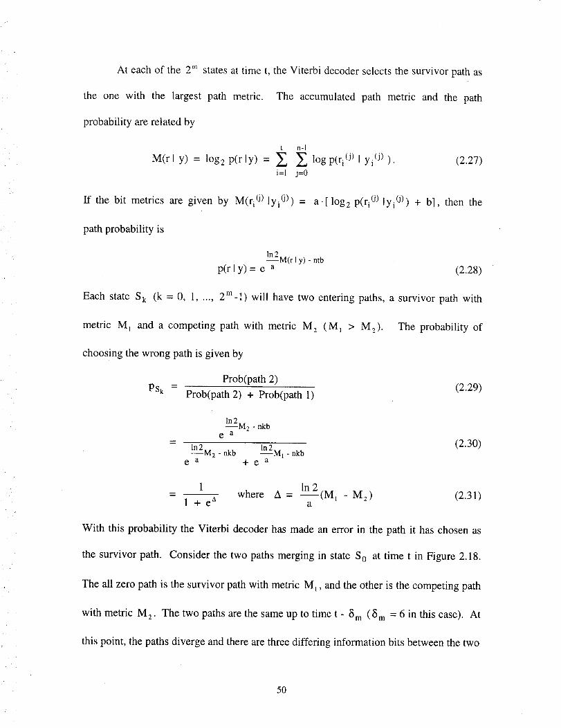
At eachof the 2m statesat time t, theViterbi decoderselectsthe survivorpathas
the one with the largest path metric.
probabilityarerelatedby
The accumulatedpath metric and the path
t n-1
M(rl y) = log 2 p(r ly) = _ _ log P(ri(J) I yi (j)).
i=l j=O
If the bit metrics are given by M(ri(J)lyiO) ) =
(2,27)
path probability is
Each state S k
a.[log 2 p(ri(J)lyiO)) + b], then the
In 2 M(r t y) - ntb
p(rly) = e a (2.28)
(k = 0, 1..... 2m-l) will have two entering paths, a survivor path with
metric M_ and a competing path with metric M2 (M_ > M2).
choosing the wrong path is given by
The probability of
Prob(path 2)
PSk = Prob(path 2) + Prob(path 1) (2.29)
ln2M 2 - nkb
e a
= (2.30)ln2M 2 - nkb ln2M_ - nkb
e a +e a
1 In 2where A- (M1 M 2) (2.31)
1 +e a a
With this probability the Viterbi decoder has made an error in the path it has chosen as
the survivor path. Consider the two paths merging in state S O at time t in Figure 2.18.
The all zero path is the survivor path with metric M_, and the other is the competing path
with metric M 2. The two paths are the same up to time t - _m (_m = 6 in this case). At
this point, the paths diverge and there are three differing information bits between the two
5O
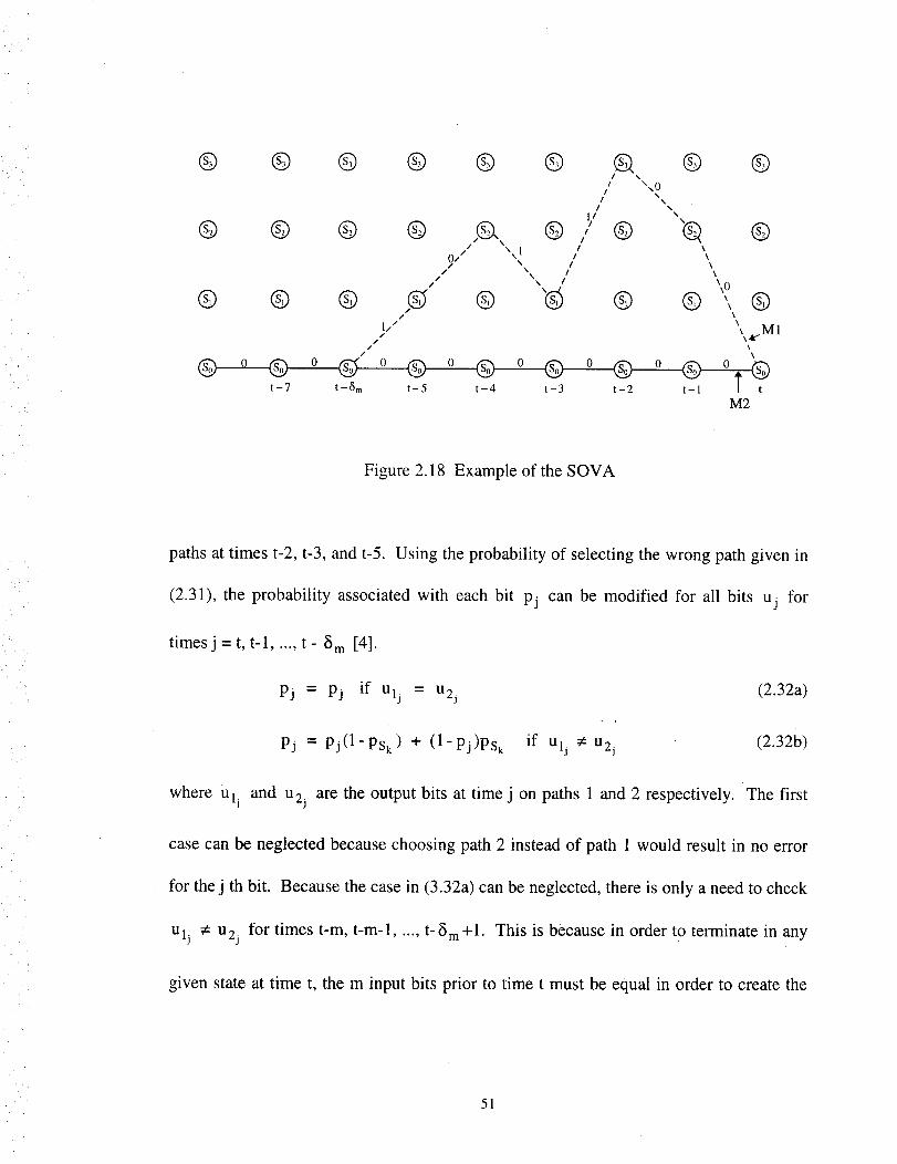
@ @ @ @ @
® ® ® ® ,,@,,Oz/ \\ 1
®
®
®I \
/I
I
I
II
// (_)!
!
!!
/
/ \ I
® ® ® ,or ® ®f
1//f
/ \
t-7 t-Sm t-5 t-4 t-3 t-2 t-I t
M2
® ®\\0
\\
N\
"Q ®\
\
\
\
\\0
® ', ®\
\
_.M1
Figure 2.18 Example of the SOVA
paths at times t-2, t-3, and t-5. Using the probability of selecting the wrong path given in
(2.31), the probability associated with each bit pj can be modified for all bits uj for
times j = t, t-1 ..... t - 8 m [4].
pj "- pj if ulj = U2j
pj = pj(1-PSk) + (1-pj)Ps k
where Ulj and u2j
(2.32a)
if ulj ¢: U2j (2.32b)
are the output bits at time j on paths 1 and 2 respectively. The first
case can be neglected because choosing path 2 instead of path 1 would result in no error
for thej th bit. Because the case in (3.32a) can be neglected, there is only a need to check
ulj _: u2j for times t-m, t-m-1 ..... t-Sm+l. This is because in order to terminate in any
given state at time t, the m input bits prior to time t must be equal in order to create the
51
given state, S k . The probability in (2.32b) can be transformed into a bit reliability. From
(2.26), the log-likelihood for the j th bit can be expressed as
1 - pjLj = log- (2.33)
Pj
This can be combined with (2.31) and (2.32) to obtain an expression for updating the
likelihood function.
Lj = log1 pj(1-Psk) + (1-pj)Psk
pj(1-ps k) + (1 Pj)Psk
= log
e A 1
- PJ(1 +e") - (1-pj) 1+ e A
e a 1
PJ(1 + e ") + (1-PJ)I + e A
1-pj a1 + --e
log pj + ezx- pjezx - log PJ
pje a + 1 -pj ea + 1 -pj
Pj
Lj log 1 + e Lj +A , .= (2.34)e A + e Lj
A good approximation of this expression is to simply take the minimum of Lj and A as
the new reliability [4].
Lj = min(Lj, A) (2.35)
For register exchange mode with truncation depth 5, each state S k will have a shift
register of 5- q bits where q-1 bits represent the magnitude of the likelihood value Lj
52
),
and one bit for the sign of L j, which corresponds to the output bit uj. The procedure
can be summarized as follows. For every state at time t, compute the path metrics for the
two paths entering state S k . Choose the path with the higher metric as the survivor path
and update the path information in the register for S k . The reliability at time t, L t is
initially set to oo. Compute the metric difference A - In 2 (M la
M2). Forj=t-m,t-
m,- 1 .... , t - _m compare the information of the two paths. If u b g: u2j, then update the
new reliability using (2.35). After the surviving paths in each state have been determined,
and the reliability information has been updated for each state, the state with the highest
path metric is determined and the reliability and output bit at t - 8 are the output for the
decoder for time t.
53

f •
Chapter 3
Simulation Techniques
Computer simulation plays an important role in the design and testing of
communications systems [5]. The results obtained from simulation can give a good
indication of how an actual system will perform under a variety of conditions.
Performance evaluation of complex communication systems using analytical techniques
can be difficult, if not impossible. Testing of the concatenated coding schemes presented
in this report using computer simulation will give an estimate of how these codes perform
under realistic conditions. In addition, the codes will be simulated using an "ideal"
AWGN channel to test how the coding systems will perform under ideal conditions.
Monte Carlo techniques were used to obtain the results for both simulations. Monte
Carlo techniques are relatively simple to implement. Data is generated at the input to the
simulation. This data is then run through the system being simulated. The data at the
output of the simulation is compared to the data at the input to determine the number of
errors. The probability of an error is simply the number of errors divided by the total
number of simulation points. To be statistically confident in the results, the simulation
should produce at least 50 errors [5]. For small values of bit error rate, a large number of
bits will be needed, which results in longer processing times. This large amount of
processing time is one of the drawbacks of using Monte Carlo techniques. The first step
54
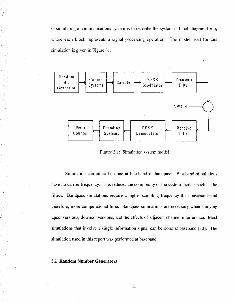
k
in simulating a communications system is to describe the system in block diagram form,
where each block represents a signal processing operation. The model used for this
simulation is given in Figure 3.1.
H amp,eBit Systems Modulator FilterGenerator
AWGN
ErrorHoeco_'ngH _ H".ceiveCounter S ystems Demodulator Filter
Figure 3.1" Simulation system model
Simulation can either be done at baseband or bandpass. Baseband simulations
have no carrier frequency. This reduces the complexity of the system models such as the
filters. Bandpass simulations require a higher sampling frequency than baseband,-and
therefore, more computational time. Bandpass simulations are necessary when studying
upconversions, downconversions, and the effects of adjacent channel interference. Most
simulations that involve a single information signal can be done at baseband [13]. The
simulation used in this report was performed at baseband.
3.1 Random Number Generators
55
i •
The various signals that exist in communication systems are random in nature.
The information signals found in communication systems typically use random voltage or
current waveforms to transmit information from one place to another. Noise is an
unwanted random signal, and causes errors in the information being sent. In order to
represent the random signals found in communication systems, a random number
generator (RNG) will be needed. Random number generators do not produce truly
random numbers, but a sequence of •"pseudo" random numbers which repeat after a
period of time. These sequences should be stationary and uncorrelated. The mean,
variance, and other parameters computed for different segments of the RNG sequence
should be equal for a RNG to be considered stationary [5]. Having a RNG with a period
less than the simulation length will cause correlation in the RNG sequence. Choosing a
RNG with a large period is desirable to avoid correlation.
3.1.1 Uniform Random Number Generator
Uniform RNG generate equiprobbile numbers within a given interval, typically
between zero and one. Uniform RNG can be generated using the following multiplicative
congruential algorithm
Ij+ 1 = a. Ij (modulus m) (3.1)
where a and m are integer constants. If a and m are chosen carefully, (3.1) will produce a
sequence of random numbers with a maximum period of m. The random number
generator used in this simulation can be found in [8] and has a very long period of
2.3 x 10¹⁸ . This is accomplished by combining two RNG sequences with
56
m1 = 2147483563
a1 = 40014
m2 = 2147483399
a2 = 40692.
In addition to a long period, this RNG passesall of the relevantstatisticaltests [8].
Assumingthe probability of a '0' and a '1' are equal, the randombit streamcan be
obtainedby usingauniform randomnumberwith thefollowing conversion
bj = 0 if Ij < 0.5
bj = 1 if Ij > 0.5
3.1.2 Gaussian Random Number Generator
There are situations that call for random numbers with different distributions, and
are typically generated by performing a transform of a uniform deviate. The generation of
Additive Gaussian White Noise (AWGN) in simulations calls for a sequence of normally
distributed random numbers. This normally distributed sequence can be generated by
using the Box Muller Method [5, 8]. If X 1 and X 2 are two independent variables with
uniform distribution between 0 and 1, then
Y1 = _t + o._/-2.1n(X1).cos(2._.X2) (3.2a)
and
Y2 = _ + 6. _/-2. ln(X 1 ). sin(2 •_. X 2) (3.2b)
are independent Gaussian variables with mean _t and standard deviation 6.
57
k
3.2 Sampling
In order to represent the signal in the simulation, the signals will need to be
sampled. The Nyquist rate of 2. B is the minimum sampling rate for bandlimited signals
of bandwidth B. For simulations, the sampling rate needs to be much higher to accurately
represent the analog signal and to reduce the affects of aliasing. The number of samples
per symbol should be an even integer between 8 and 16. Having the number of samples
per symbol greater than 16 is not necessary for most simulations [13].
3.3 Filters
In Communication systems, filters are needed for the purposes of bandlimiting
signals and rejecting out of band noise. The filtering in the process can produce
something known as intersymbol interference.
3.3.1 Intersymbol Interference
Consider the effects of passing a series of impulses spaced T b seconds apart
through a low pass filter. Each impulse produces its own output from the filter. The
output from one pulse extends into the output of pulse that starts T b seconds later. This
is known as Intersymbol Interference (ISI) and it can produce errors at the receiver.
The effects of ISI can be avoided by an appropriate choice of a low pass filter.
Nyquist proposed a technique that theoretically produces zero ISI. This is accomplished
by creating in the receiver a pulse that resembles the sin x/x shape, crossing the axis at
58
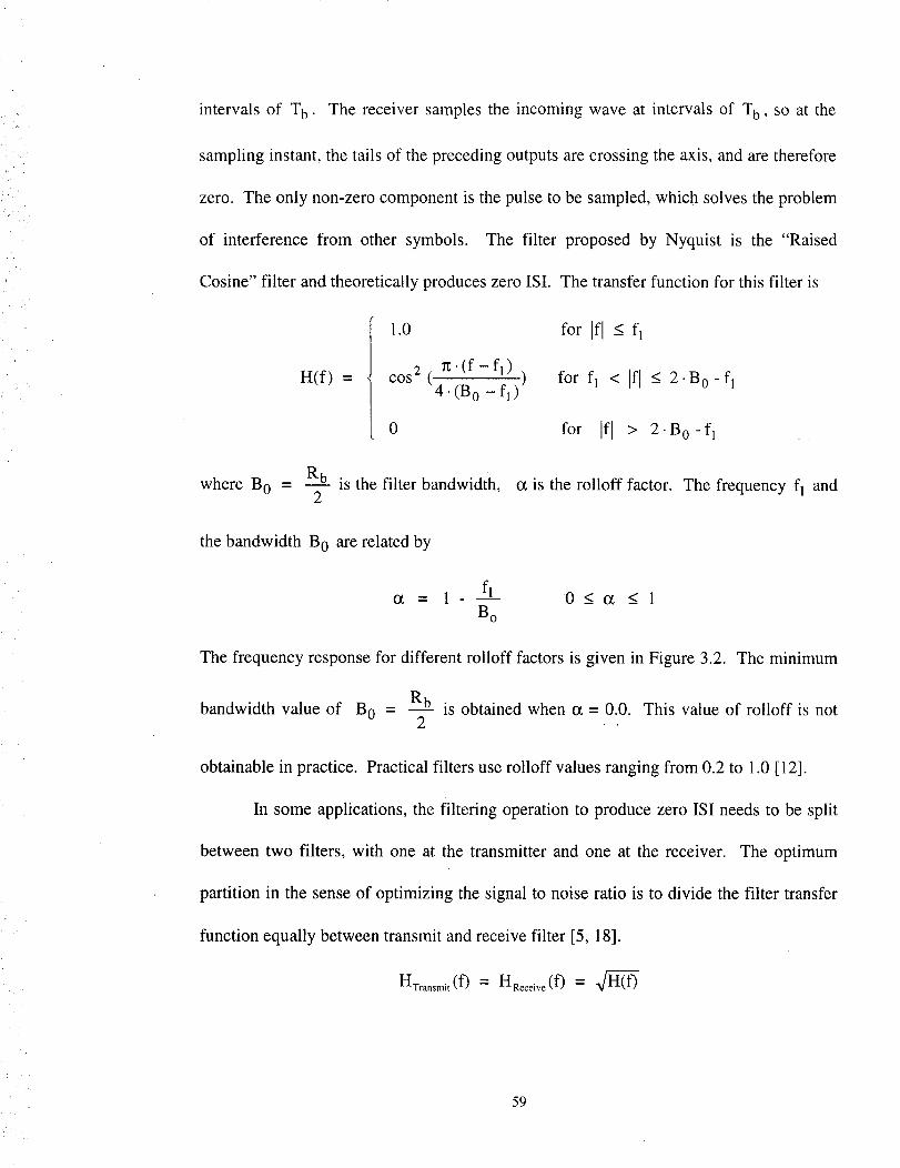
intervalsof Tb. The receiversamplesthe incomingwave at intervalsof Tb, so at the
samplinginstant,thetailsof theprecedingoutputsarecrossingtheaxis,andaretherefore
zero. Theonly non-zerocomponentis thepulseto besampled,which solvestheproblem
of interferencefrom other symbols. The filter proposedby Nyquist is the "Raised
Cosine"filter andtheoreticallyproduceszeroISI. Thetransferfunctionfor this filter is
1.0
ft. (f - fl )
H(f) = cos 2 (4_[-_o-_);))
0
where B 0 = R----kis the filter bandwidth,2
the bandwidth B 0 are related by
for If] < fl
for fl < If] -< 2. B o -fl
for ]f] > 2.B o-fl
ot is the rolloff factor. The frequency fl and
= 1 - fl 0 < (x < 1
Bo
The frequency response for different rolloff factors is given in Figure 3.2. The minimum
bandwidth value of B 0 - Rb is obtained when a = 0.0. This value of rolloff is not2 . •
obtainable in practice. Practical filters use rolloff values ranging from 0.2 to 1.0 [12].
In some applications, the filtering operation to produce zero ISI needs to be split
between two filters, with one at the transmitter and one at the receiver. The optimum
partition in the sense of optimizing the signal to noise ratio is to divide the filter transfer
function equally between transmit and receive filter [5, 18].
HTransmit(f) -" HR_i_(f ) =
59
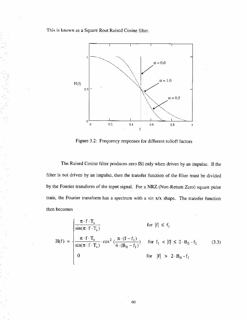
This is known as a Square Root Raised Cosine filter.
H(f)
0.5
I I I I
_=0.0
_=1.0
o I I0 0.2 0.4 0.6 0.8
f
Figure 3.2: Frequency responses for different rolloff factors
The Raised Cosine filter produces zero ISI only when driven by an impulse. If the
filter is not driven by an impulse, then the transfer function of the filter must be divided
by the Fourier transform of the input signal. For a NRZ (Non-Return Zero) square pulse
train, the Fourier transform has a spectrum with a sin x/x shape. The transfer function
then becomes
H(f) =
•f. T sfor If[- fl
sin(n;, f. T s )
7z'f'T s . rt'(f-f 1)•cos 2 for fl < Ifl < 2.B o fl (3.3)
sin(_:, f •Ts) I',_: iB-o_t'i )' - -
0 for Ifl > 2.Bo -fl
60
where Ts is the symbol period. Note that the raisedcosinefilter is bandlimitedto
Rs •(1+ c_),andatf = Rs, x/sinx goesto infinity. Therefore,for thissystemto work,o_2
mustbelessthan1.0[12].
3.3.2 Digital Filters
In this simulation, filters will be needed for the purpose of band limiting signals,
producing zero intersymbol interference (ISI), and rejecting out of band noise. Because
this simulation is in discrete time, digital filters will be needed to accomplish the above
objectives. There are two major types of digital filter design methods: Infinite Impulse
Response (I/R), and Finite Impulse Response (FIR). Both have advantages and
disadvantages, and neither is best for all situations. The optimal filter design method
must be determined by analyzing the requirements and objectives of the application.
The ]JR method uses the widely available filter functions from analog filter
theory. This method starts with an analog filter transfer function, and then translates this
analog function in such a way that makes it suitable for discrete-time systems. Filters
designed using the IIR method will be recursive in nature (the output of the filter depends
on previous filter outputs, as well as past and current values of the input), and the filter's
impulse response will be infinite. IIR filters require fewer coefficients than FIR filters,
and have a closed form design technique that does not require iteration. Some of the
• disadvantages of ]JR filters include non-linear phase response, and the use of feedback in
the implementation that can cause instability if not carefully implemented.
61
The FIR method does not rely on analog filter theory. Instead the frequency
response of the desired filter is used to determine the digital filter coefficients. This
design method is non-recursive in nature, and the impulse response has a finite number of
terms. Filters designed using the FIR method are always stable, and have a linear phase.
FIR filters need a high number of coefficients to adequately describe the impulse response
of the filter. This large number of filter coefficients results in longer processing times,
and can be a great disadvantage if used in real time applications. In addition, the design
procedure may need to be performed numerous times to find the optimum number of
coefficients to meet the requirements of the application.
For this simulation, Square Root Raised Cosine filters will be used on the
transmitting and receiving end of the system. These filters are defined by the frequency
response in Equation 3.3. Using FIR filter design, the filter can be designed directly from
the filter response, whereas in IIR design, an appropriate analog filter containing poles
and zeros is needed to begin the design. In addition, Raised Cosine filters need linear
phase to achieve zero ISI [12]. Using FIR filters, linear phase can be achieved. The only
drawback to the design of Square Root Raised Cosine filter using FIR method is the large
number of coefficients needed to achieve an accurate magnitude response. For this
simulation FIR filter design method will be used to design the Square Root Raised Cosine
filter. The filter coefficients were generated using a program written in Mathcad.
• 3.3.3 FIR Filter Design of Transmit Filter
62
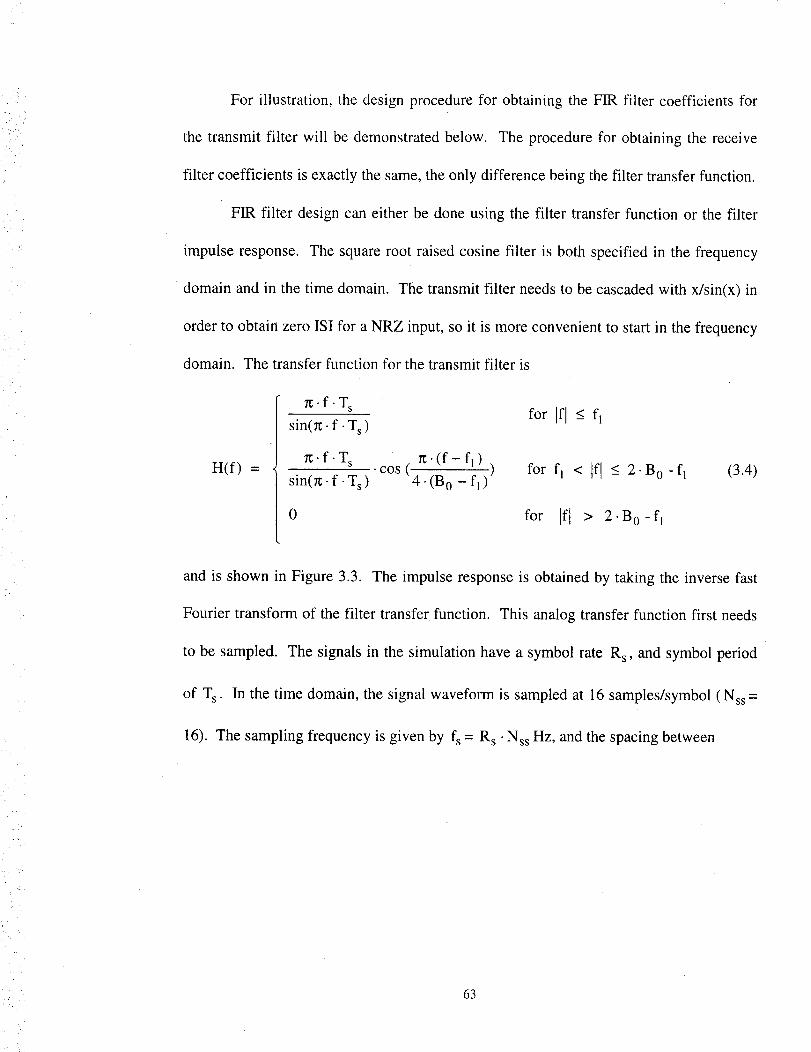
For illustration, the designprocedurefor obtainingthe FIR filter coefficientsfor
thetransmit filter will bedemonstratedbelow. The procedurefor obtainingthe receive
filter coefficientsisexactlythesame,theonly differencebeingthefilter transferfunction.
FIR filter designcaneitherbedoneusingthefilter transferfunction or the filter
impulseresponse.Thesquareroot raisedcosinefilter is bothspecifiedin the frequency
domainandin thetime domain. Thetransmitfilter needsto becascadedwith x/sin(x) in
orderto obtainzeroISI for aNRZ input,so it is moreconvenientto startin thefrequency
domain. Thetransferfunctionfor thetransmitfilter is
_'f'Ts for Ifl < flsin(_; • f. T s )
_f'Ts _'(f- fl)
H(f) = sin(_.f.Ts).COS(4.(Bo _fl)) for fl < Jfl < 2Bo-fl (3.4)
0 for If[ > 2.B 0 - fl
and is shown in Figure 3.3. The impulse response is obtained by taking the inverse fast
Fourier transform of the filter transfer function. This analog transfer function first needs
to be sampled. The signals in the simulation have a symbol rate R s, and symbol period
of T s . In the time domain, the signal waveform is sampled at 16 samples/symbol (Nss =
16). The sampling frequency is given by fs = Rs •Nss Hz, and the spacing between
•IZ¸
63
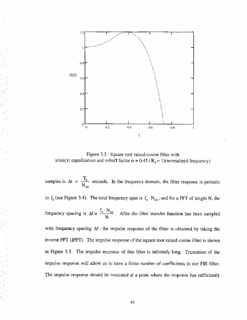
H(f)
1.2
0.8
0.6
0.4
0.2
\\
\
I I I \ I
0.2 0.4 0.6 0.8
Figure 3.3: Square root raised cosine filter with
x/sin(x) equalization and rolloff factor o_- 0.45 ( R s = 1)(normalized frequency)
samples is At - Ts seconds. In the frequency domain, the filter response is periodicNss
in fs (see Figure 3.4). The total frequency span is fs "Nss, and for a FFT of length N, the
frequency spacing is Af = fs" Nss After the filter transfer function has been sampledN
with frequency spacing Af, the impulse response of the filter is obtained by taking the
inverse FFT (IFFT). The impulse response of the square root raised cosine filter is shown
in Figure 3.5. The impulse response of this filter is infinitely long. Truncation of the
impulse response will allow us to have a finite number of coefficients in our FIR filter.
The impulse response should be truncated at a point where the response has sufficiently
64
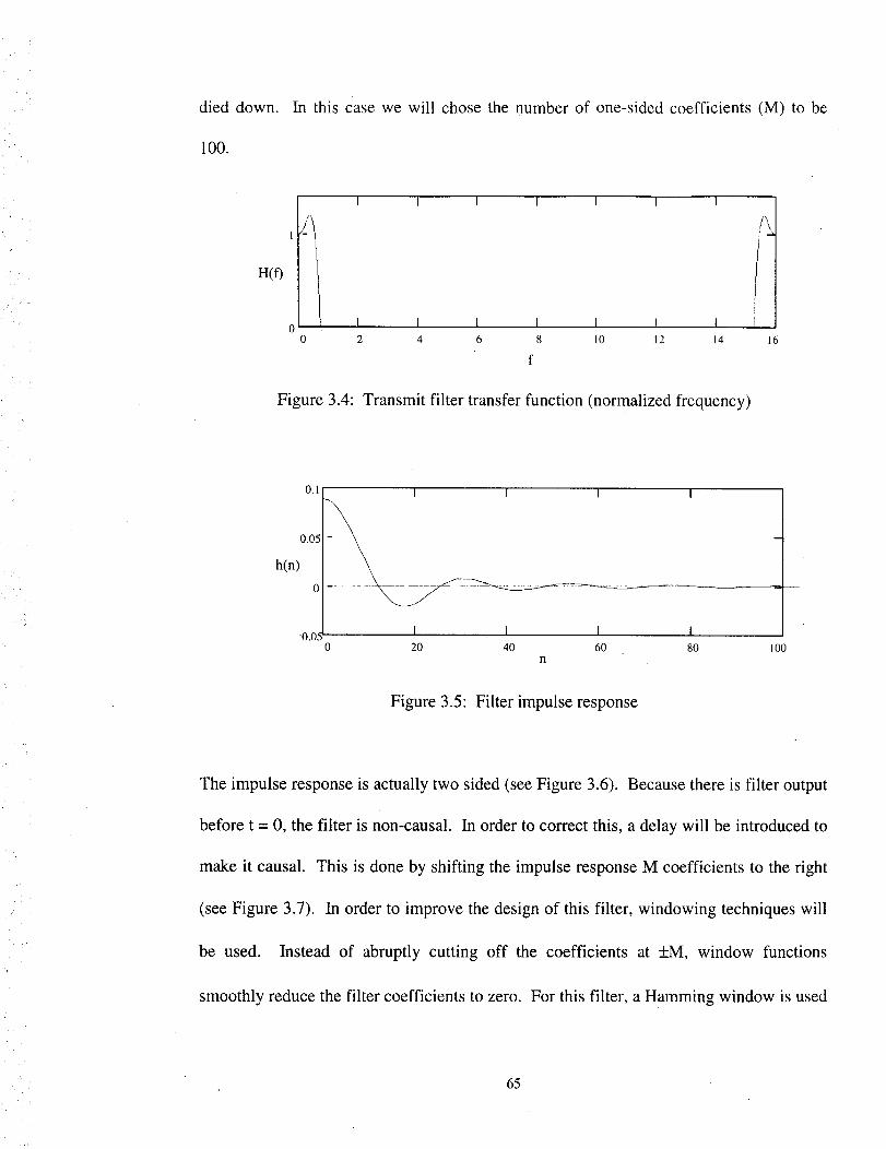
died down.
100.
In this casewe will chosethe numberof one-sidedcoefficients(M) to be
H(f)
00
I I I I I I I
I I I I I I I2 4 6 8 10 12 14
f
16
Figure 3.4: Transmit filter transfer function (normalized frequency)
0,1
0.05
h(n)
0
-0.0_*
i I I I
i
I I I I0 20 40 60 80 100
Figure 3.5: Filter impulse response
The impulse response is actually two sided (see Figure 3.6). Because there is filter output
before t = 0, the filter is non-causal. In order to correct this, a delay will be introduced to
make it causal. This is done by shifting the impulse response M coefficients to the right
(see Figure 3.7). In order to improve the design of this filter, windowing techniques will
be used. Instead of abruptly cutting off the coefficients at +_M, window functions
smoothly reduce the filter coefficients to zero. For this filter, a Hamming window is used
65
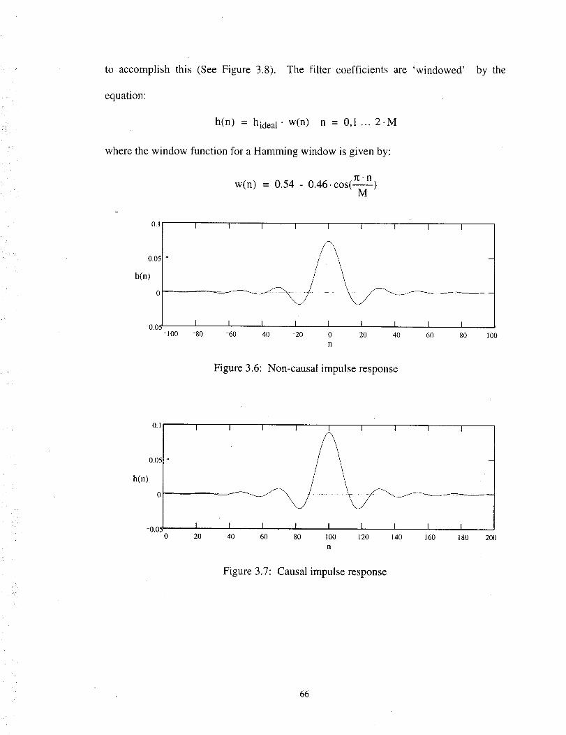
to accomplishthis (SeeFigure 3.8). The filter coefficients are 'windowed'
equation:
h(n) = hideaI • w(n) n = 0,1 ... 2.M
wherethewindow functionfor aHammingwindow is givenby:
by the
0.05
h(n)
0
-0.0
w(n) = 0.54 - 0.46.cos(-_)
I I I I I I I I I
I I I I I I I I I100 -80 -60 40 20 0 20 40 60 80 100
n
Figure 3.6: Non-causal impulse response
0.1
0.05
h(n)
-0.05
I I I I I I I I I
I I I I I I I I I0 20 40 60 80 100 120 140 ! 60 180 200
n
5
Figure 3.7: Causal impulse response
66
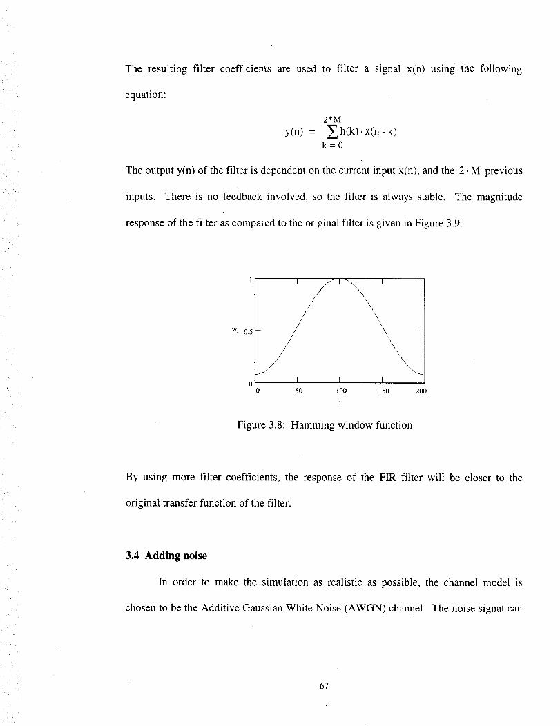
i!The resulting filter coefficients are used to filter a signal x(n) using the following
equation:
y(n) =
2*M
h(k)' x(n - k)k=0
The output y(n) of the filter is dependent on the current input x(n), and the 2. M previous
inputs. There is no feedback involved, so the filter is always stable. The magnitude
response of the filter as compared to the original filter is given in Figure 3.9.
wi 0.5
I0
I
I I50 100 150 200
i
Figure 3.8: Hamming window function
By using more filter coefficients, the response of the FIR filter will be closer to the
original transfer function of the filter.
3.4 Adding noise
In order to make the simulation as realistic as possible, the channel model is
chosen to be the Additive Gaussian White Noise (AWGN) channel. The noise signal can
67
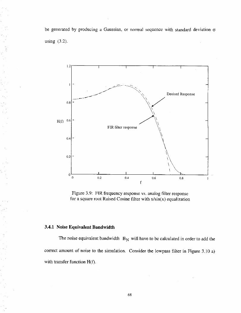
be generated by producing a Gaussian, or normal sequence with standard deviation
using (3.2).
H(t)
1.2
O.8
0.6
0.4
0.2
I I I I
\,./
FIR filter response _\
- /l
I I I
0 0.2 0.4 0.6 0.8
f
Desired Response
m
w
Figure 3.9: FIR frequency response vs. analog filter response
for a square root Raised Cosine filter with x/sin(x) equalization
3.4.1 Noise Equivalent Bandwidth
The noise equivalent bandwidth B N will have to be calculated in order to add the
correct amount of noise to the simulation.
with transfer function H(f).
Consider the lowpass filter in Figure 3.10 a)
68
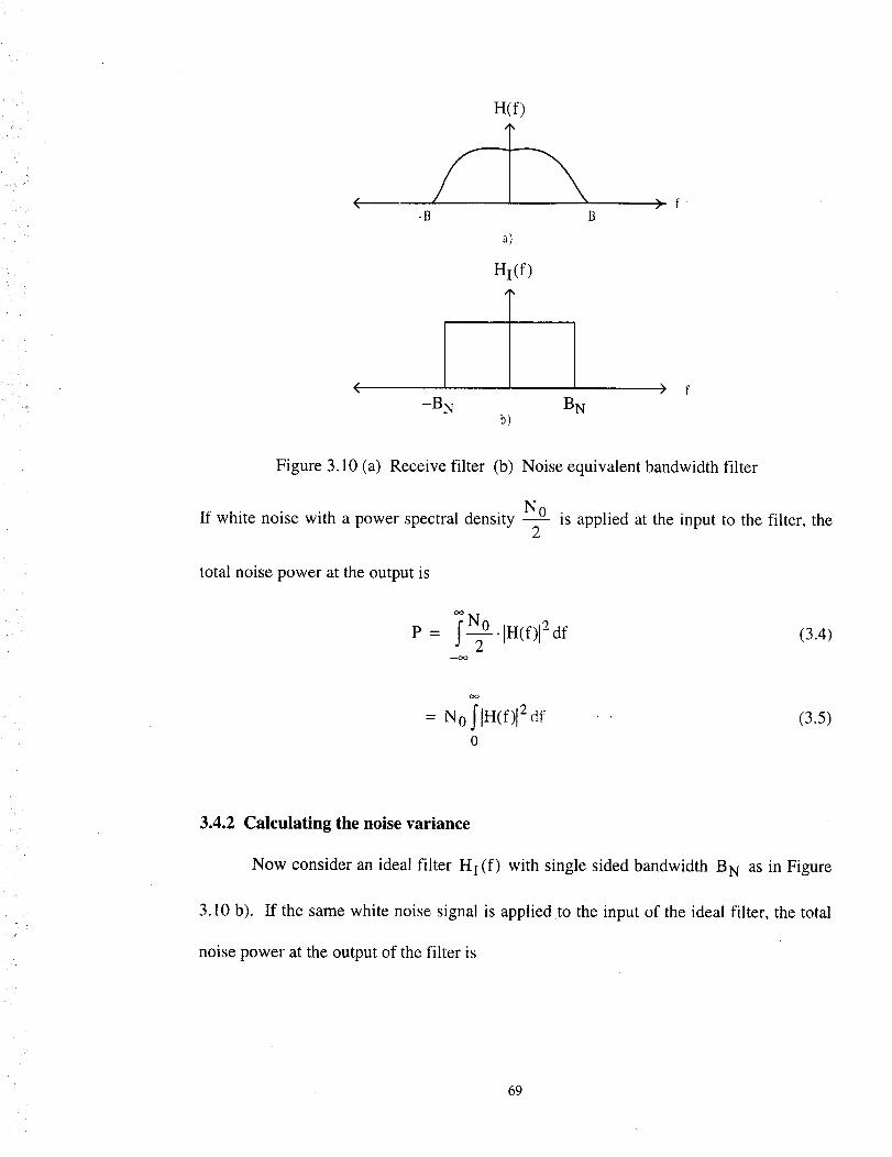
(
f
H(f)
( _/f--_'__ > f
-B B
a)
H(f)
( ) f-B N B N
b)
Figure 3.10 (a) Receive filter (b) Noise equivalent bandwidth filter
If white noise with a power spectral density --NO is applied at the input to the filter, the2
total noise power at the output is
P= f _---9-0•[H(f)[2 df (3.4)
oO
= N O lH(f)[ e df
0
(3.5)
3.4.2 Calculating the noise variance
Now consider an ideal filter H I (f) with single sided bandwidth B N as in Figure
3.10 b). If the same white noise signal is applied to the input of the ideal filter, the total
noise power at the output of the filter is
69
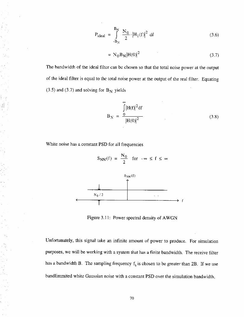
BNNo
. Hi(f) 2 df (3.6)Pideal = ; T-B N
!_i ' /
= NoBNIH(0)I 2 (3.7)
The bandwidth of the ideal filter can be chosen so that the total noise power at the output
of the ideal filter is equal to the total noise power at the output of the real filter. Equating
(3.5) and (3.7) and solving for B N yields
Iln(f)12df
BN_ 0 (3.8)In(O)l2
White noise has a constant PSD for all frequencies
SNN(f)- NO for-oo2
_<f<oo
SNN (f)
N O / 2 , ,
( T ) f
Figure 3.11: Power spectral density of AWGN
,H
?
Unfortunately, this signal take an infinite amount of power to produce. For simulation
purposes, we will be working with a system that has a finite bandwidth. The receive filter
has a bandwidth B. The sampling frequency fs is chosen to be greater than 2B. If we use
bandlimmited white Gaussian noise with a constant PSD over the simulation bandwidth,
7O
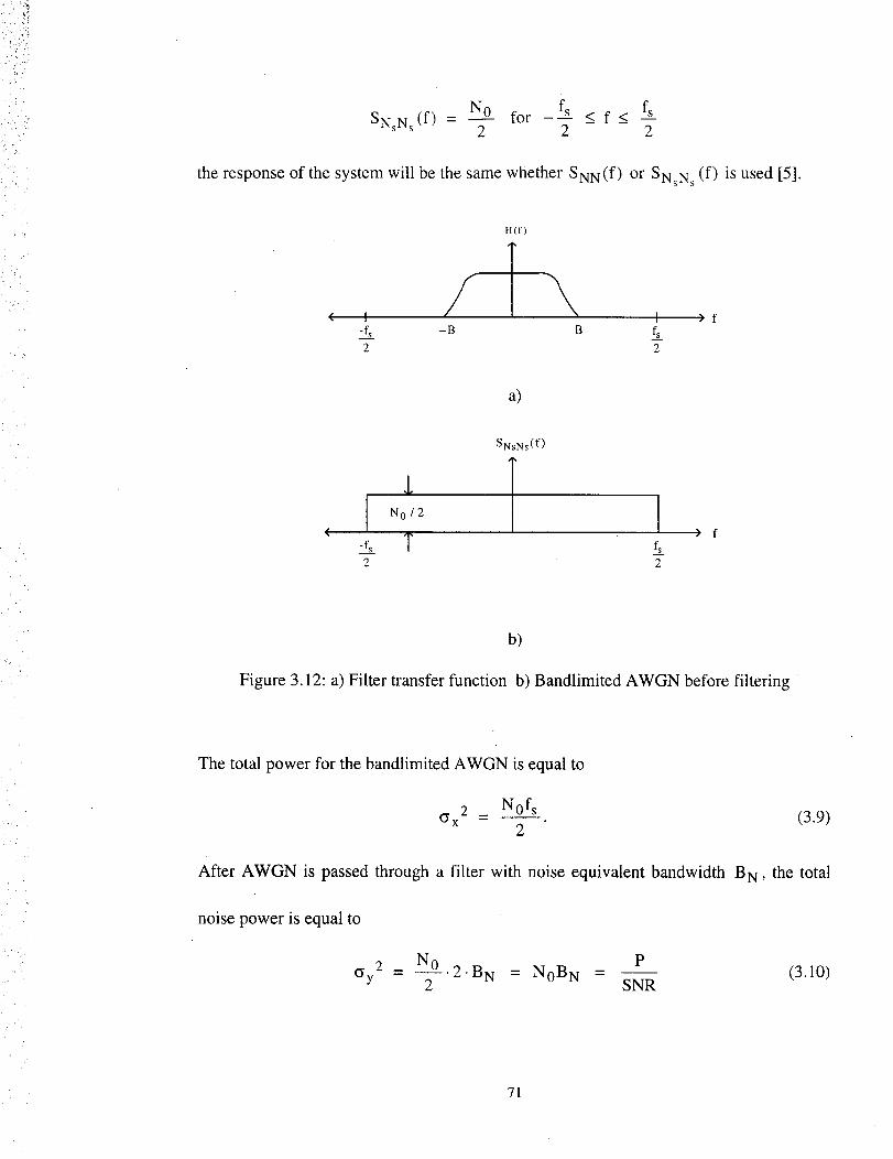
i/,i?i>
,-)
N____Q_O fsSN_N (f).. = for < f <2 2 2
the response of the system will be the same whether SNN(f ) or SNsNs (f) is used [5].
H(f)
a)
{No/2
-fs m2
SNsNs(f)
l) f
2
b)
Figure 3.12: a) Filter transfer function b) Bandlimited AWGN before filtering
The total power for the bandlimited AWGN is equal to
2 Nofscyx - (3.9)
2
After AWGN is passed through a filter with noise equivalent bandwidth B N , the total
noise power is equal to
N O P--.2.B N = NoB N - (3.10)
2 SNR
71

whereP is the total signalpowerandSNR is thesignalto noiseratio. Combining(3.9)
2and(3.10)andsolving for cyx
(yx2 _ P fs (3.11)SNR 2' BN
(yx2is the total noisepowerthat is to beaddedto the channelbeforethe Rx filter. The
noisecanbegeneratedby using(3.2) to createa sequenceof Gaussianrandomvariables
with la= 0 and _ = cyx.
Sometimesit is convenientto expressthe probability of a bit error Peasa
Ebfunctionof p -
NOwhereEb is thebit energyand NOis thenoisedensity.The noise
variancewill beexpresseddifferentlythan(3.11).
_ EbLet p- --. In terms of N0
NO
NOEb
P(3.12)
The signal power P is equal to
mE s E b .k
Ts Ts(3.13)
where k is the number of bits per symbol. From (3.13), the energy per bit is
p • Y sE b -
k(3.14)
2_ N0fsThe total noise power before filtering is equal to c_x
2from Figure 3 b).
Combining this with (3.12) and (3.14) yields
72
2_ P'Ts'fs (3.15)2.9.k
The sampling frequency is defined as
so (3.16) can be rewritten as
fs = Rs "Nss (3.16)
2 _ P'Nss(Yx (3.17)
2.9.k
The noise can be generated by using (3.2) to create a sequence of Gaussian random
variables with g = 0 and _ = _x-
3.4.3 Ideal Channel model
An ideal channel can be used to obtain results that are not degraded by the filters.
There is no need to simulate the analog signal, and modulate, filter, and add noise. The
binary data can have Gaussian noise added directly to the data bits, and then these bits
can either be soft or hard decoded. For each binary bit u j, the noise corrupted bit can be
obtained by using (3.2) with la = 1 for Uj -" 1, and la = -1 for Uj = 0. The variance of the
noise is
where 9 is the signal to noise ratio.
I_ 2 1
29
For hard decisions V j, if the noise corrupted uj is
greater than zero, then Vj "" 1.
obtained.
Otherwise, Vj = 0. Using this method, ideal BPSK is
73
3.5 Simulation Results
The simulation was run without coding systems to verify the simulation was
working properly. The results were compared to the theoretical BPSK results, which are
given by
pe = 1.erfc( E/-_/
2 _._/No J
where E b is the energy per bit, N o is the single sided noise power spectral density, and
2 i e-U2/2 duerfc(x) = -_-_" x
The results of the simulation are shown in Figure 3.13. Looking at the results of the
simulation, two observations can be made. First, for greater values of E b /No, the
simulation results deviate from the theoretical curve. This can be attributed to the effects
of filtering. Second, for higher values of rolloff, the performance of the simulation
becomes closer to the theoretical. This can be attributed to the increase in bandwidth
which comes from an increase in the rolloff value.
74
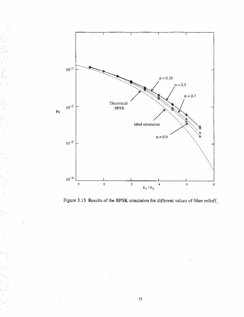
Pe
10 -1
lO -2
10-3
I I I I
Theoretical
BPSK
c_ = 0.35
Ideal simulation
\10 -4 I I I I
-2 0 2 4 6 8
E h / N o
Figure 3.13 Results of the BPSK simulation for different values of filter rolloff.
75
Chapter 4
Erasure Methods and Simulation Results
The purpose of this chapter is to investigate the performance of the concatenated
system given in Figure 1.1, and to discuss and propose methods of declaring RS symbol
erasures to improve performance. It is the goal of these methods to recognize symbols
that are in error and erase them, thus utilizing the full capacity of the errors and erasures
Reed Solomon decoder. The success of these methods is highly dependent on being able
to successfully identify the errors in each Reed Solomon codeword (RSW). The
performance of the concatenated system without erasures was tested. In addition, a basic
method for erasure declaration using the reliability information provided by the SOVA
was implemented. This method is based on [14]. Two new procedures for declaring
erasures are proposed. Both use the reliability information from the SOVA in addition to
information provided by successfully decoded RSW in the deinterleaving frame. The
results of these two methods are presented and compared to Paaske's [7] method.
4.1 Concatenated system simulation results
The performance of the concatenated system presented in Figure 1.1 was
investigated. More specifically, the concatenated system used by NASA for deep space
communication has been simulated. This system uses a rate 1/2, K = 7 convolutional
76
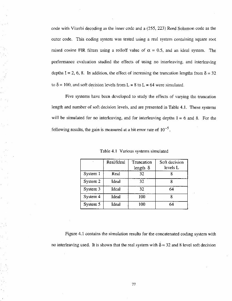
codewith Viterbi decodingasthe innercodeanda (255,223) ReedSolomoncodeasthe
outer code. This coding systemwas testedusing a real systemcontainingsquareroot
raisedcosine FIR filters using a rolloff value of o_= 0.5, and an ideal system. The
performanceevaluationstudied the effects of using no interleaving,and interleaving
depthsI = 2, 6, 8. In addition,theeffectof increasingthetruncationlengthsfrom 8 = 32
to 8 = 100,andsoft decisionlevelsfrom L = 8 to L = 64weresimulated.
Five systemshavebeendevelopedto studythe effectsof varyingthe truncation
lengthandnumberof soft decisionlevels,andarepresentedin Table4.1. Thesesystems
will be simulatedfor no interleaving,and for interleavingdepthsI -- 6 and 8. For the
following results,thegain is measuredatabit errorrateof 10.5 .
Table4.1 Varioussystemssimulated
Real/Ideal Truncation Soft decisionlength 5 levelsL
System1 Real 32 8
System2 Ideal 32 8
System3 Ideal 32 64
System4 Ideal 100 8
System5 Ideal 100 64
no
Figure 4.1 contains the simulation results for the concatenated coding system with
interleaving used. It is shown that the real system with 5 = 32 and 8 level soft decision
77
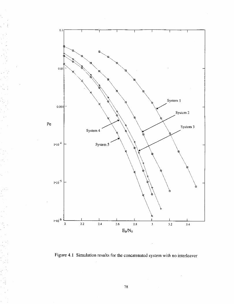
I I I I I I I
o.0o I
System 1
System 2
Pe
System 4
System 5
System 3
1"10 `6 I I I I I I
2.2 2.4 2.6 2.8 3 3.2 3.4
Ebmo
Figure 4.1 Simulation results for the concatenated system with no interleaver
78
Viterbi decoding (system 1) results in a loss of about 0.3 dB when compared with the
ideal system with the same truncation length and soft decision levels (system 2). There is
approximately a gain of 0.2 dB when the decision depth 8 is increased from 8 - 32 to 8 =
100. This can be illustrated in Figure 4.1 by comparing the difference in performance
between system 2 (8 = 32, L = 8) and system 4 (8 = 100, L = 8). Likewise, there is also a
0.2 dB gain when the decision depth in system 3 is increased from 8 = 32 to 8 - 100 to
form system 5. When the number of soft decision levels is increased from L = 8 in
system 2 to L = 64 in system 4, the result is about a 0.15 dB gain. Likewise, the increase
in soft decision levels from system 3 to system 5 results in roughly 0.15 dB gain. The
combined use of 8 = 100 and L = 64 results in about 0.35 dB gain over the ideal system
using 8 = 32 and L = 8. These gains are consistent for interleaving depths I = 6 (Figure
4.2) and I = 8 (Figure 4.3).
The benefits of using an interleaver is demonstrated in Figure 4.4, where the
simulation results for system 5 using no interleaving, and depths I = 2, 6, and 8 are
presented. It has been shown that the use of interleaving depth I = 2 can provide
approximately 0.2 dB gain over the system using no interleaving. When the interleaving
depth is increased from I = 2 to I = 6, there is an additional gain of slightly more than 0.2
dB, for a total of roughly 0.4 dB over the system using no interleaving. The use of an
interleaver with depth I = 8 provided a minor gain over the system using I = 6. The total
gain of using I = 8 when compared to the non-interleaved system is approximately 0.45
dB. It should also be noted that the concatenated coding system using interleaving depths
greater than 8 resulted in little or no improvement over the system using depth I = 8.
79
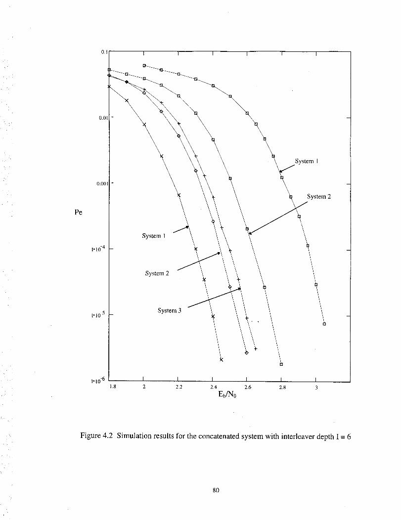
• if! _
Pe
0.00 l -
1.10-4
1"10-5 -
I I I I I I
System 1
\
System 2
System 3
\\
\ !
System i
1.10-6 I I I I I I
1.8 2 2.2 2.4 2.6 2.8 3
Eb/No
System 2
\//
I
/ Figure 4.2 Simulation results for the concatenated system with interleaver depth I = 6
8O
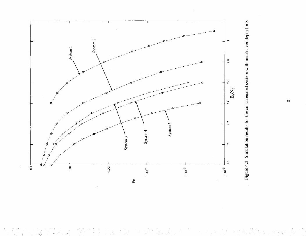
I I 1 I
r_
t_
c_
II
°_
°_
E
C#3
c_
0
L_
o
c_
O
c_
o_
_o
: i _ :
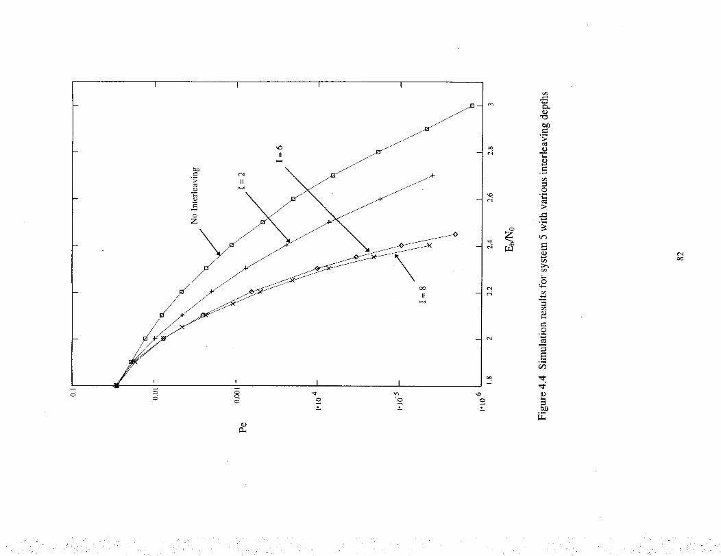
o
I I i I
II
If
C_
b_
°_
L_
°_
0
c_
o_
T_
C)
bO
oo
. i _,_, _',_i,_ _ ,.... _,_.
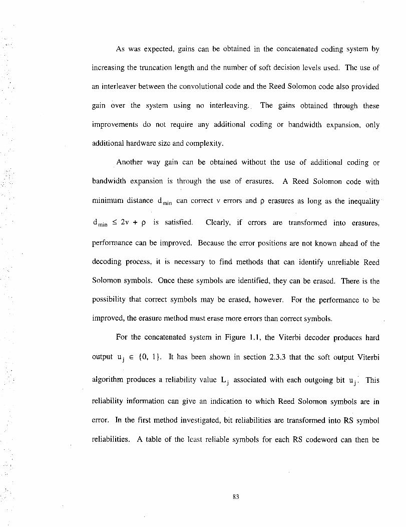
As wasexpected,gainscan be obtainedin the concatenatedcoding systemby
increasingthe truncationlengthandthenumberof soft decisionlevelsused. The useof
an interleaverbetweentheconvolutionalcodeandtheReedSolomoncodealsoprovided
gain over the system using no interleaving. The
improvementsdo not require any additional coding
additionalhardwaresizeandcomplexity.
gains obtained through these
or bandwidth expansion,only
Another way gain can be obtained without the use of additional coding or
bandwidth expansionis through the use of erasures. A Reed Solomoncode with
minimum distance d min can correct v errors and 9 erasures as long as the inequality
dmi n < 2v + 9 is satisfied. Clearly, if errors are transformed into erasures,
performance can be improved. Because the error positions are not known ahead of the
decoding process, it is necessary to find methods that can identify unreliable Reed
Solomon symbols. Once these symbols are identified, they can be erased. There is the
possibility that correct symbols may be erased, however. For the performance to be
improved, the erasure method must erase more errors than correct symbols.
For the concatenated system in Figure 1.1, the Viterbi decoder produces hard
output uj e {0, 1 }. It has been shown in section 2.3.3 that the soft output Viterbi
algorithm produces a reliability value Lj associated with each outgoing bit ujl This
reliability information can give an indication to which Reed Solomon symbols are in
error. In the first method investigated, bit reliabilities are transformed into RS symbol
reliabilities. A table of the least reliable symbols for each RS codeword can then be
83
compiled,andthe leastreliablesymbolscanbeerased.
erasuresin presentedin greaterdetailbelow.
The first methodfor declaring
4.2 Erasure Method 1
The first methodfor declaringRSsymbolerasuresis basedon the methodfound
in [14]. The SOVA is usedto obtain the reliabilities of each output bit from the Viterbi
decoder. The output of the SOVA is quantized using q+l bits, where q bits represent the
magnitude of the decision (the reliability), and 1 bit represents the hard decision. In
general, these reliabilities are real valued, and have a range between 0 and infinity. It is
not necessary to quantize the reliability values between 0 to infinity, but rather between 0
and some value Lma x . The reliability values produced by the SOVA will be assigned one
of 2 q levels between 0 and Lma x. If a reliability is greater than Lmax, then the
reliability level is set to 2 q (i.e. the maximum level). For this simulation q = 8 and
Lma x = 8 were used. From here on out, the "reliability value" Lj for a bit will refer to
the q-bit quantized level.
Before declaring RS symbol erasures, the bit reliabilities from the output of the
SOVA need to be converted to RS symbol reliabilities. This can be accomplished by
simply using the minimum bit reliability in a symbol as the symbol reliability. This can
be rationalized as follows. If a bit has a small reliability, and is in error, the symbol will
be in error also. Therefore, the best information contained in the symbol reliability is
contained in the minimum bit reliability. For each RS codeword (RSW), a reliability
table (RT) is formed. The RT has m e positions, where m e is the maximum number of
84
?!
erasures allowed. If the least reliable symbols in the RSW occur at positions k j, where j
= 1, 2 ..... m e, then RT(j) = kj. RT(1) contains the least reliable position, RT(2)
contains the 2nd least reliable symbol, etc. The RS decoder will first attempt to decode
without declaring erasures. If this is a successful decoding, stop. If not, the two symbols
with the smallest reliabilities are erased (RT(1) and RT(2)), and decoding is attempted
again. If successful, decoding stops. If unsuccessful, the four least likely symbols are
erased (RT(1) through RT(4)) and decoding is attempted again. For each unsuccessful
decoding, two more erasures are declared until either a successful decoding is achieved,
or the maximum number of erasures m e is reached. This maximum number is chosen to
be 16 erasures. Using more than 16 erasures gave poorer results due to the fact that the
symbols reliabilities at the output of the SOVA hit more correct symbols than errors. In
addition, the probability of a decoding error is also increased. A decoding error occurs
when a codeword contains more than t errors, and fails to notice that it does. The decoder
claims that there are less than t errors. This is different than a decoding failure. A
decoding failure happens when there are more than t errors, and the decoder detects that it
contains more than t errors. For a t error correcting RS code, the probability of a
decoding error is I/t! [7, 14, 19]. The procedure for erasure decoding using Method 1 is
presented below.
4.2.1 Procedure for erasure decoding using Method 1
The decoding of each RS codeword involves the following steps:
1. Set the number of erasures n e = 0.
85
2. Attemptto decodetheRScodewordusingerrorsonly decoding.If successful,stop.
3. Set ne- ne +2.
4. Erasethe ne leastreliablesymbolsasdeterminedby the reliability table,andattempt
erroranderasuresdecoding.If successful,stop.
5. If ne = me(themaximumnumberof erasuresallowed),thenstop.
6. Goto step3.
7. Stop.
4.2.2 Simulation Results for Method 1
The results of the simulation for Method 1 are presented in Figures 4.5 through
4.7. These figures contain the results using system 1, 2, and 5 for no interleaving (Figure
4.5), and interleaving depths I = 6 (Figure 4.6) and I = 8 (Figure 4.7). The results of the
corresponding concatenated code using no erasures is also presented for comparison
purposes. From these figures, it is evident that the use of erasure Method 1 results in
approximately O.1 dB gain over the non-erasure concatenated system. This result was
consistent regardless of the truncation length, number of soft decision levels_ and
interleaving depth used by the concatenated system. It should be noted that the gains
obtained by using different interleaving depths with erasure Method 1 were identical to
the gains obtained when using different interleaving depths in the standard concatenated
system. In addition, it should also be noted that increasing the decision depth and number
of soft decision levels for the systems simulated using erasure Method 1 were consistent
with the results for the concatenated system presented in section 4.1.
86
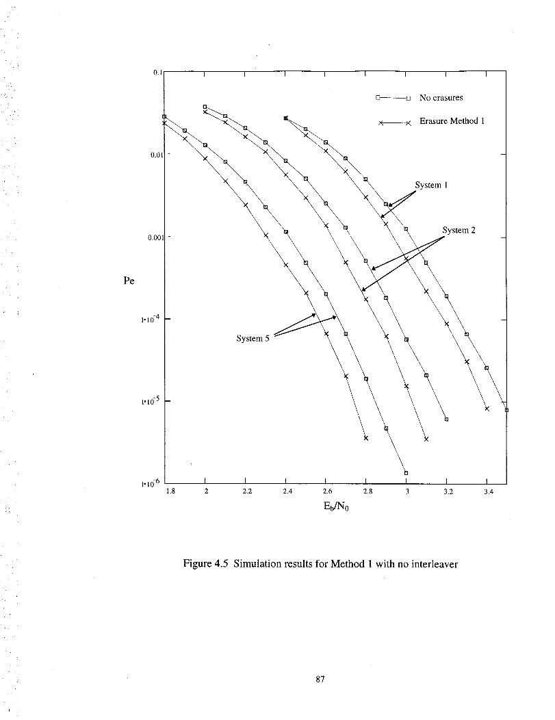
'), ,
Pe
o.o
0.001
1.10-4
t.165
1.10-6
I I I I I I I I
\ '\
No erasures
Erasure Method 1
System 1
System 2
System 5
\
I I I t I I I I
1.8 2 2.2 2.4 2.6 2.8 3 3.2
Eu/No
3.4
Figure 4.5 Simulation results for Method 1 with no interleaver
87
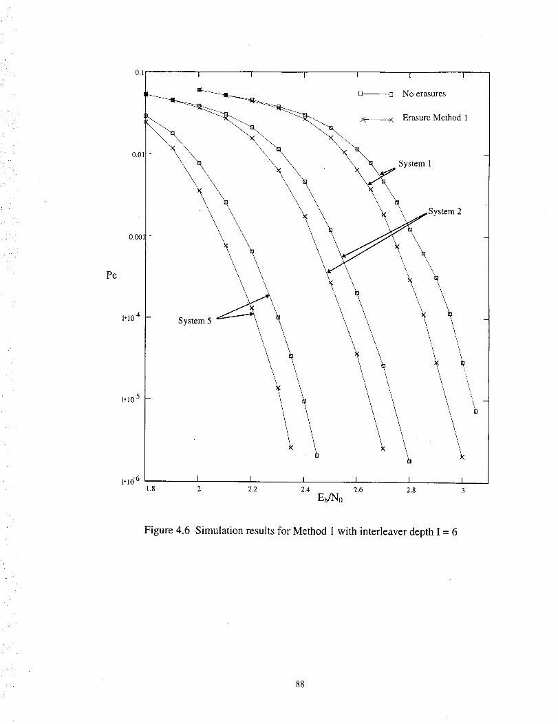
Pe
I i
No erasures
Erasure Method 1
System 1
stem 2
1.10 4
1.10-6
\
\
System 5
\
I I I I I I
1.8 2 2.2 2.4 2.6 2.8 3
Eb/No
\\
Figure 4.6 Simulation results for Method 1 with interleaver depth I = 6
88
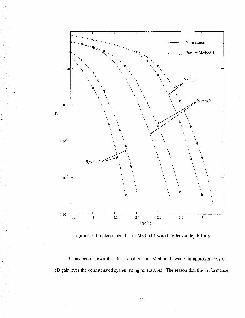
I I I I I
No erasures
Erasure Method 1
Pe
0.001
System 1
,stem 2
1.10_4
l.lo-5
System 5
\ \\ \
\\
1.10-6 I I I I I I,1.8 2 2.2 2.4 2.6 2.8 3
Eb/No
Figure 4.7 Simulation results for Method 1 with interleaver depth I = 8
It has been shown that the use of erasure Method 1 results in approximately 0.1
dB gain over the concatenated system using no erasures. The reason that the performance
89
7" i
!:i "
is not greatly increased is because the erasure declaring process is not optimal. In general,
when erasing two symbols at a time, gain is only achieved when both erased symbols are
errors (GE). If only 1 erasure is a GE, the capacity of the code stays the same, and if
neither erasure is a GE, then capacity of the code actually decreases. Method 1 uses the
reliability information generated from the SOVA, and the symbols with the smallest
reliabilities are systematically erased. A symbol with a small reliability does not
guarantee a GE. For example, the smallest reliability value (Lj = 0) occurs when there is
a metric difference A -- 0. Because the path metrics are equally likely, the probability the
wrong path has been chosen is 0.5. This is why a small reliability value does not
guarantee a wrong path has been taken. The reliability table used in Method 1 can be
modified to give more reliable information. This can be accomplished by using decoded
Reed Solomon codewords in the deinterleaving frame to provide information to the non-
decoded Reed Solomon codewords. This information can be used to construct a
reliability table with more accurate information, and then the unreliable symbols can be
converted into RS symbol erasures. The second method for declaring erasures is
presented below.
4.3 Erasure Method 2
It has been found that the burst errors at the output of the SOVA contain the same
reliabilities within the burst. Consider the two paths merging in state S k at time t in
Figure 4.8. The survivor path has metric M 1 and the competing path has metric M 2.
90

Competing Path
Metric M 2
• /t-8 m Sk
Bit Reliabilities AALj ALjLjA ALjAALj ALjA ALjLjALjLjALjALjAALjLjLjLj t
Symbol A A A AReliabilities
Figure 4.8 The updating of symbol reliabilities in the SOVA
The reliabilities Lj on the surviving path in the SOVA are updated by selecting the
minimum between Lj and A, where A is the difference between the two paths merged in
state Sk . When the bit reliabilities are converted to symbol reliabilities, the minimum bit
reliability is chosen as the symbol reliability. Assuming that A is the minimum and this
is part of the surviving path, then consecutive symbols in the surviving path have
identical reliabilities. In the standard Viterbi decoder, error events occur when at time t
the decoder chooses the wrong path. This is also what happens in the SOVA. If the path
with the maximum metric is the wrong path, then all of the reliabilities for the differing
bits will be equal to A. If this is the path selected by the SOVA as the output of the
decoder, then the reliability will be equal for the length of the burst. It is apparent from
Figure 4.8 that all symbol reliabilities in the erroneous path are equivalent. This
information can be used to distinguish error paths and declare erasures, and can be
91
accomplishedby usinga methodsimilar to the one proposedby Paaske. Assumethat
after an initial decodingattemptof a deinterleavingframe,someof theRSW havebeen
successfullydecoded,while othershave not. The error positions in the successfully
decodedcodewordsareknown. Usingthe aboveobservation,if aneighboringsymbolin
anundecodedRSWhasanidenticalreliability valueasthecorrectedsymbolin adecoded
RSW,it is highly probablethatthatsymbolis alsoanerrorandcanbeerased.
As mentioned previously, a symbol with a low reliability value does not
necessarilydenotea symbolerror. FromFigure4.8, it canbeseenthat if A is small,then
it maybecontainedin thereliability tablefor a non-decodedRSW.Assumethat a RSW
is decodedand the error positionsare known. The correctpositionsarealso known.
These correct positions can be used to eliminate other correct symbols from being
includedin the reliability tablefor non-decodedRSW. If the neighboringpositionsof a
correct symbol havethe samereliability, then it is highly probablethat this symbol is
correctalso. Theprocedurefor erasuredecodingusingMethod2 is summarizedbelow.
A deinterleavingflame with interleavingdepthI containsI RSW. Decodingof
eachRSW in theframeis first attempted usingMethod 1. For eachRSW,a tableof the
least reliable symbols is compiled,and for eachunsuccessfuldecodingattempt,two
additional symbolsareerased,anddecodingis attemptedagain. This processcontinues
until either a successfuldecodingoccurs,or a maximum amountof erasureshasbeen
reached.If lessthanI codewordsaresuccessfullydecoded,redecodingis attempted.The
RT usedin Method 1containsthe leastreliablesymbolsasdeterminedby the outputof
the SOVA. The reliability table can be modified using information provided by the
92
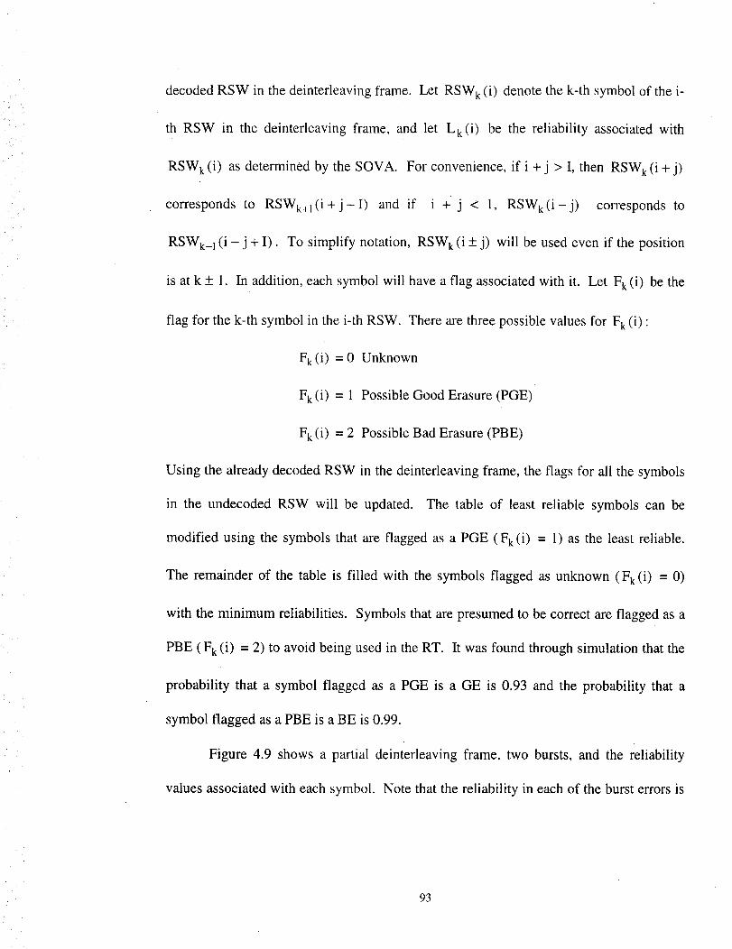
decodedRSW in thedeinterleavingframe. Let RSW k (i) denote the k-th symbol of the i-
th RSW in the deinterleaving frame, and let Lk(i ) be the reliability associated with
RSW k (i) as determined by the SOVA. For convenience, if i + j > I, then RSW k (i + j)
corresponds to RSWk+ 1 (i + j - I) and if i + j < l, RSW k (i - j) corresponds to
RSWk_ 1(i - j + I). To simplify notation, RSW k (i __ j) will be used even if the position
is at k + 1. In addition, each symbol will have a flag associated with it. Let F k (i) be the
flag for the k-th symbol in the i-th RSW. There are three possible values for F k (i) :
Fk(i ) = 0 Unknown
F k (i) = 1 Possible Good Erasure (PGE)
F k (i) = 2 Possible Bad Erasure (PBE)
Using the already decoded RSW in the deinterleaving frame, the flags for all the symbols
in the undecoded RSW will be updated. The table of least reliable symbols can be
modified using the symbols that are flagged as a PGE (Fk(i) = 1) as the least reliable.
The remainder of the table is filled with the symbols flagged as unknown (F k (i) = 0)
with the minimum reliabilities. Symbols that are presumed to be correct are flagged as a
PBE (F k (i) = 2) to avoid being used in the RT. It was found through simulation that the
probability that a symbol flagged as a PGE is a GE is 0.93 and the probability that a
symbol flagged as a PBE is a BE is 0.99.
Figure 4.9 shows a partial deinterleaving frame, two bursts, and the reliability
values associated with each symbol. Note that the reliability in each of the burst errors is
93
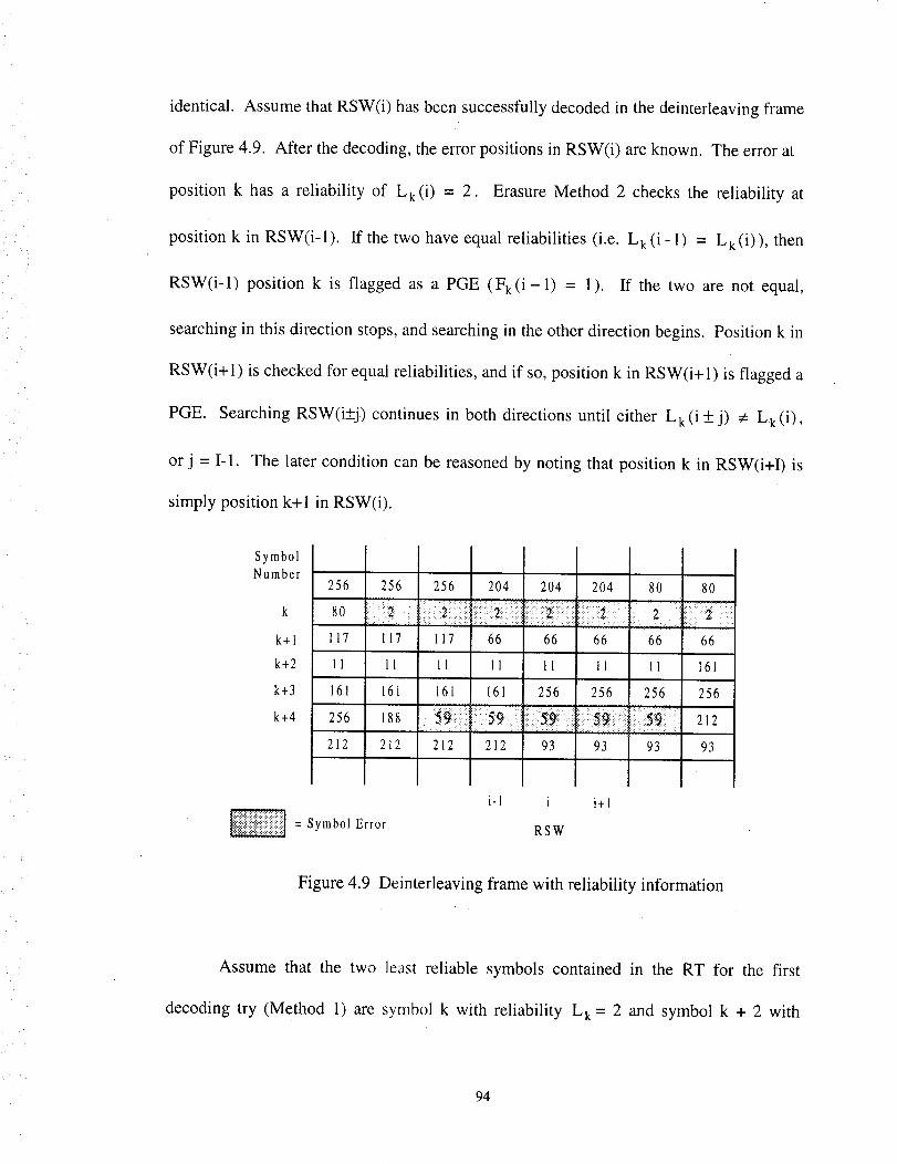
identical. Assume that RSW(i) has been successfully decoded in the deinterleaving flame
of Figure 4.9. After the decoding, the error positions in RSW(i) are known. The error at
position k has a reliability of Lk(i) = 2. Erasure Method 2 checks the reliability at
position k in RSW(i-1). If the two have equal reliabilities (i.e. Lk(i- 1) = Lk(i)), then
RSW(i-1) position k is flagged as a PGE (Fg(i-1) = 1). If the two are not equal,
searching in this direction stops, and searching in the other direction begins. Position k in
RSW(i+I) is checked for equal reliabilities, and if so, position k in RSW(i+I) is flagged a
PGE. Searching RSW(i_+j) continues in both directions until either L k (i _+ j) _ L k (i),
or j = I-1. The later condition can be reasoned by noting that position k in RSW(i+I) is
simply position k+l in RSW(i).
SymbolNumber
k
k+l
k+2
k+3
k+4
256
80
117
11
161
256
212
256
117
11
161
188
212
256
117
11
161
204
66
11
161
204
66
11
256
204
66
11
256
8O
66
11
256
212 212 93 93 93
80
66
161
256
212
93
i-I i i+l
= Symbol Error RSW
Figure 4.9 Deinterleaving frame with reliability information
Assume that the two least reliable symbols contained in the RT for the first
decoding try (Method 1) are symbol k with reliability Lk = 2 and symbol k + 2 with
94
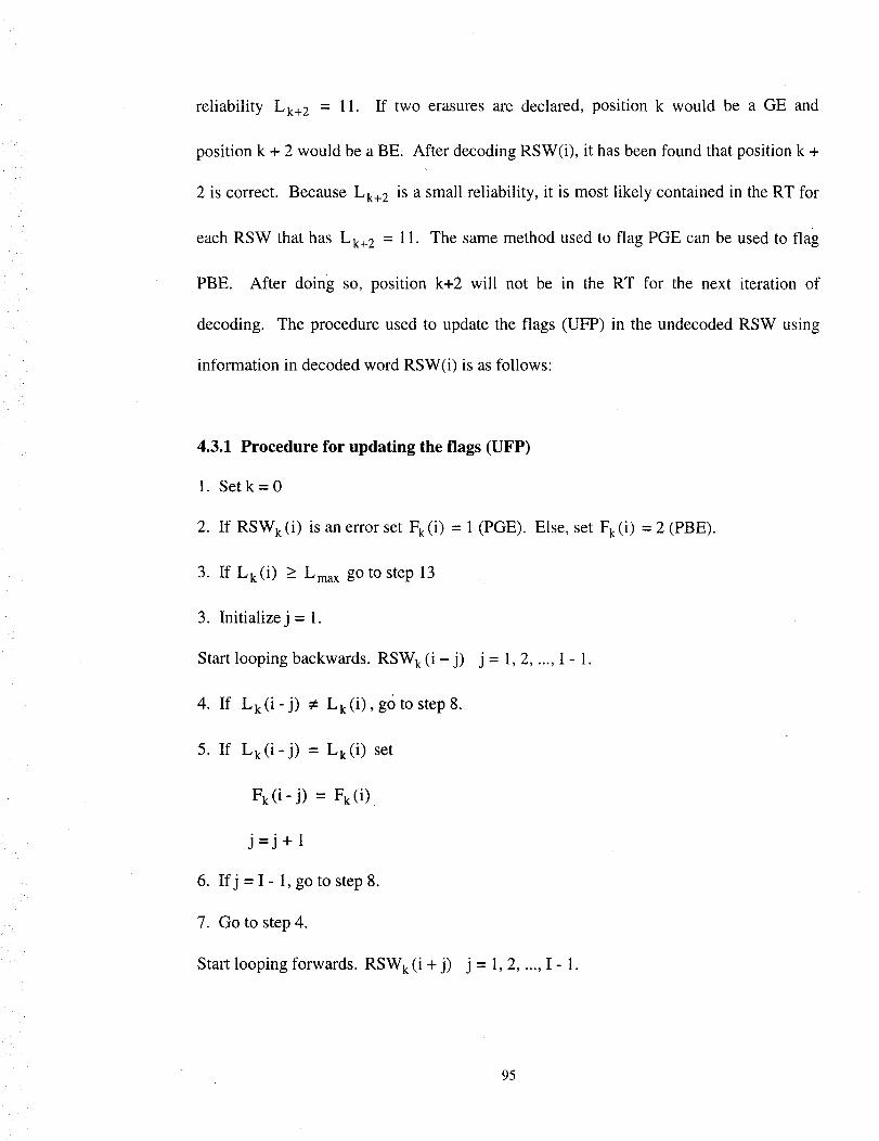
reliability Lk+2 = 1 1. ff two erasures are declared, position k would be a GE and
position k + 2 would be a BE. After decoding RSW(i), it has been found that position k +
2 is correct. Because Lk+ 2 is a small reliability, it is most likely contained in the RT for
each RSW that has Lk+ 2 = 1 1. The same method used to flag PGE can be used to flag
PBE. After doing so, position k+2 will not be in the RT for the next iteration of
decoding. The procedure used to update the flags (UFP) in the undecoded RSW using
information in decoded word RSW(i) is as follows:
4.3.1 Procedure for updating the flags (UFP)
1. Set k=0
2. If RSW k (i) is an error set F k (i) = 1 (PGE). Else, set F k (i) = 2 (PBE).
3. If Lk(i) > Lma x go to step 13
3. Initialize j = 1.
Start looping backwards. RSW k (i - j)
4. If L k(i-j) _ L k(i), go to step 8.
j=l,2 ..... I-1.
5. If Lk(i-j) = Lk(i ) set
F k (i - j) = Fk (i)
j=j+l
6. If j = I - 1, go to step 8.
7. Go to step 4.
Start looping forwards. RSW k (i + j) j=l,2 ..... I-1.
95
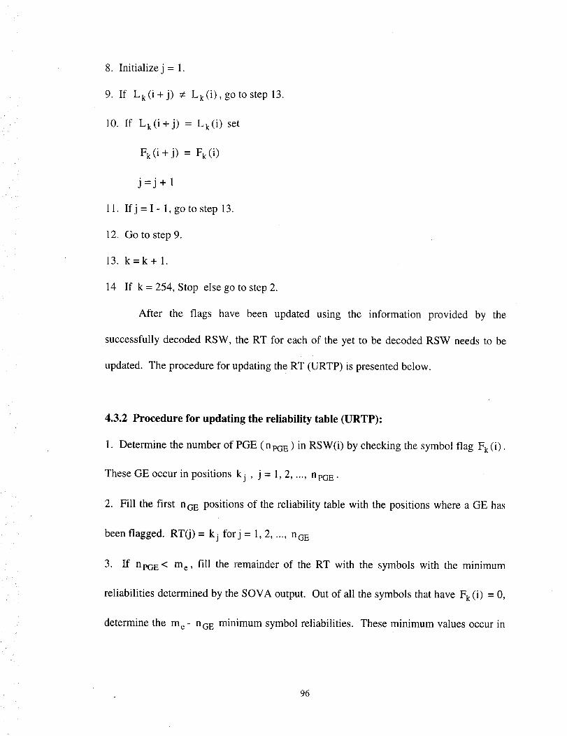
8. Initializej = 1.
9. If Lk(i+j) ¢: Lk(i),gotoste p 13.
10. If L k(i+j) = L k(i) set
F k(i+j) = F k(i)
j-j+l
11. Ifj=I-l,gotostepl3.
12. Go to step 9.
13. k=k+ 1.
14 If k = 254, Stop else go to step 2.
After the flags have been updated using the information provided by the
successfully decoded RSW, the RT for each of the yet to be decoded RSW needs to be
updated. The procedure for updating the RT (URTP) is presented below.
4.3.2 Procedure for updating the reliability table (URTP):
1. Determine the number of PGE ( npG E ) in RSW(i) by checking the symbol flag Fk (i).
These GE occur in positions kj , j = 1, 2 ..... npG E .
2. Fill the first nGE positions of the reliability table with the positions where a GE has
been flagged. RT(i) = kj forj = 1, 2 ..... nGE
3. If npG E < me, fill the remainder of the RT with the symbols with the minimum
reliabilities determined by the SOVA output. Out of all the symbols that have Fk (i) = 0,
determine the m e- nGE minimum symbol reliabilities. These minimum values occur in
96
positions k e, g = 1, 2 ..... m e- npG E . Fill the remaining m e- npG E positions in RT
with the symbols with the minimum reliabilities. RT(nGE + 1) = ke, g = 1, 2, ..., m e-
n PGE •
The procedure for decoding using Method 2 is presented below.
4.3.3 Procedure for decoding using Method 2
1. Attempt initial decoding using Method 1.
2. Set i d = number of correctly decoded RSW.
3. If i d = I, go to step 9.
4. If i d = 0, go to step 9.
5. For each decoded codeword, declare flags in the undecoded RSW using UFP.
6. For each non decoded codeword, update the reliability table using URTP.
7. Attempt decoding using Method 1 with the updated RT.
8. If step 7 yields at least one successfully decoded RSW, go to step 2.
9. Stop.
/t
4.3.4 An example of erasure decoding using Erasure Method 2
As an example, consider the deinterleaving frame in Figure 4.10. This frame was
simulated at a signal to noise value of E b / N O = 1.9 dB. The error positions are denoted
by the shaded areas, and the reliability values are given. This frame contains 8 RSW with
a total of 161 symbol errors. It should be noted that each RSW in the deinterleaving
frame contains more than 16 errors. If no erasure information was used, every RSW in
97
the flame would fail to decode. The reliability table for each RSW in the flame for the
first iteration is presented in Figure 4. i 1, where the reliability value and symbol position
are given (L k, k). In addition, the number of decoding trials for each codeword is also
shown. The RT is initially formed by using the minimum reliabilities generated by the
SOVA. For the first iteration, decoding of each RSW is attempted using Method 1.
RSW(1) successfully decodes after 6 decoding trials using 10 erasures. RSW(3) is
successfully decoded after declaring 4 erasures (3 decoding trials), and RSW(8) decodes
using 2 erasures (2 decoding trials). All other RSW fail to decode after 9 decoding trials
apiece. Now, the RT is modified by updating the flags using UFP, and the updated RT is
compiled using URTP giving the symbols with flag = 1 (PBE) the highest priority in the
table. The modified RT is in Figure 4.12. Decoding is attempted again using Method 1
with the updated RT. For this iteration, RSW(2) decoded successfully using 14 erasures
(8 decoding trials), RSW(4) using 12 erasures (7 trials), and RSW(7) using 8 erasures (5
trials). Decoding attempts for RSW(5) and RSW(6) are once again unsuccessful. The
flags for RSW(5) and RSW(6) are updated using the information provided by RSW(2),
RSW(4), and RSW(7). The updated RT is generated using the updated flags, and is
presented in Figure 4.13. Decoding is attempted again using Method 1. RSW(5) is
decoded using 16 erasures (9 decoding trials), and RSW(6) is decoded using 14 erasures
(8 decoding trials). Erasure Method 2 required a total of
successfully decode this frame. This results in an average of
RSW.
11 1 decoding trials to
13.9 decoding trials per
98
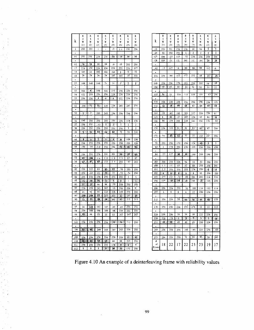
R R R R R R R R
S S S S S S S S
k w w w w w w w w
(i) (2) (3) (4) (5} (6) (7) (8)
3 256 256 I 1 t3 211 231) 256
[0 256 256 256 256 :!:_i: iii::39 i::i 39_ I ,_9
16 ii::l_ : ::1._ IO IO IO IO 256 256
17 256 254 254 256 256 256 256 207
18 105 21 105 184 184 i 2 /" _3 79
19 79 79 79 79 107 1()7 I117 256
27 140 14()140 74 74
33 166 ::ii:_. 166 166 237 256 256 256
34 122 218 256 256 256 256 256 256
35 256 256 122 256 256
42 256 iii ?_ii :i ::i!i_.:._:: 169 256 21)3 2113 256
52 245 245 256 256 256 256
56 190 256 256 256 256 256 178 178
57 256 256 19(1 3 _ i::: 2 2 2:o5: ,,
58 256 256 256 256 256 256 5 5
59 !_ii_i::i ii:_iii :.:.:.i8_:.:. !!gi: _i _i:: 72 72 23!
I66 i !i::i::i_::i::::::i::::i::_:::::: i::;i!_::ii::i :::.;:51::::i::i::i::::121::i: i::_:, t69 256
67 256 256 256 256 256 256 256 126
68 194 194 210 256 256 iii: _1_i il t iii_ _!i!i: i_iii::
: ]
74 256 256 256 2{)1 201 i_!! i 9¢_!i !ii_Oi'
75 i)ii_i! !ii_!_il 116 116 116 116 67 67
76 ii::_::!i iii6"_i_i ::$_i::i 173 219 256 187 2(13
82 256 222 83 i_?_i! ii!_ill !78 256 256
83 256 169 122 :::.::_i:.:::. 73 179 179 256
84 256 256 . 256 256 256 256 6 ,,,6,
85 i::_¢;iliiiii_(_iiii::l::::::i_i::::::!_i::i ii_i;!_:i!iii*iii:i _ i:_:._::_::_::i::!i86 !ii_::i::i:: ::!::;_.ii;::! 94 94 179 256 256 256
87 256 256 243 243 116 256 256 91
88 9I 91 91 224 228 228 256 256
90 !!i_ :i!ili_ili i;_.: i!_ii!i!iii!i6_! i iii:_i!il 2t5 2t5
97 26 :. _i_i 145 145 165 165 256 256
98 256 168 168 168 168 234 256 256
99 ::i_ili :: 44 53 53 53 163 247 247
11)3 256 256 256 256 ii::ii)_i:i i_i_::_ Ill 256
106 ii_i::ii::ii::ii_iiii 249 249 249 249 256 256
109 256 256 256 254 256 256 :i ?_i_:i__._ii '_!_iiiii
IlO _iiii_iiii::Ii_i ::::i_ii_i 68 68 " 203 256
Ill _ 256 _ 256 " 256 " 25"6 178 iiiii_;::_i@ii _iiiili 9
112 9 9 9 ::i::;::_!::i!::i::_:._::i :, i::ii_ =] 172 256
R R R R R R R R
S S S S S S S S
k w w w w w w w w(11 (21 (3) 141 151 (6_ (71 18t
125 256 231 256 256 3(} 31} _ j';
t26 30 256 256 _ _ _ , 2 , _ 1:. :_127 IO0 127 157 175 256. 256 256 256
128 [89 IO[ I01 H)I IOI IO[ 2i1 i 2_
I42 117 117 141 190 _ 90:: 9,0 113 161
144 256 189 177 177 252 i 25 25:_, _i
149 256 256 256 !93 256 256 19 ,:: 19=
151) [ 9:] 19: ! 9 _ii 3t 3i 3l 22
157 51 118 119 119 119 1811 256
161) 256 256 256 256 256 256 256 126
1611 i:.ii:._:ii I _i:i: 6_< .: _!_: 69 !i 691 i 69_ii 6_
164 251 185 185 185 222 256 256 81
165 81 8_:1:/ 137 2117 256 97 86 ::i_38,, ;
[66 86 119 2118 2511 24t 154 154 11)2
171t 256 193 111.51. ii : 51 i 5i:-i, _}i?ii:; 97 256
.:-:_::-: .:-.x-_;.:176 72 :.: _ .,:: : :.: :.:.:.:.:. 77 77 _69 201 256
179 256 256 172 256 124 :;i _ i, 5
18(} 5 174 256 256 256 256 256 256
184 t27 127 :._i ! 3,_i! 108 244 2,14 256
189 256 256 256 96 33 33 256 256
190 I11 II1 57 57 255 256 20l
_91 Z!5 2_6 2_6 256 256 256 U_I iii::i_192 ii::iii_i:;[::ii_ii::_i i_iiii 6; i!i 6' 95 256 256
193 233 172 172 185 201 2111 114 114
19,4 119 iiiii_!i!"il)[_i?'ilillt "iiiil(l i'}_:i:i 146 256............... rrrr'r
206 256 256 256 136 169 169 162 114
2117 6 6 6 6 22 256 256 256
212 256 256 66 :i:166 !ii_i::il i166! _:: _:,i::i 159
218 256 256 256 256 256 11 tl 115
229 256 256 39 39 39 133 256 1256
230 256 174 i::i::!_::::i 3ii::i_i:,i _ i ili:-_
231 :: l_; iiiii_!iii: 49 49 49 256 256 256
249 256 256 256 185 185 225 256 i?i _$::
'253 256 256 256 31 iii31i 3_ :i_i:31. 200
#
or 18 22 17 22 23 23 19 17Errors
Figure 4.10 An example of a deinterleaving frame with reliability values
99
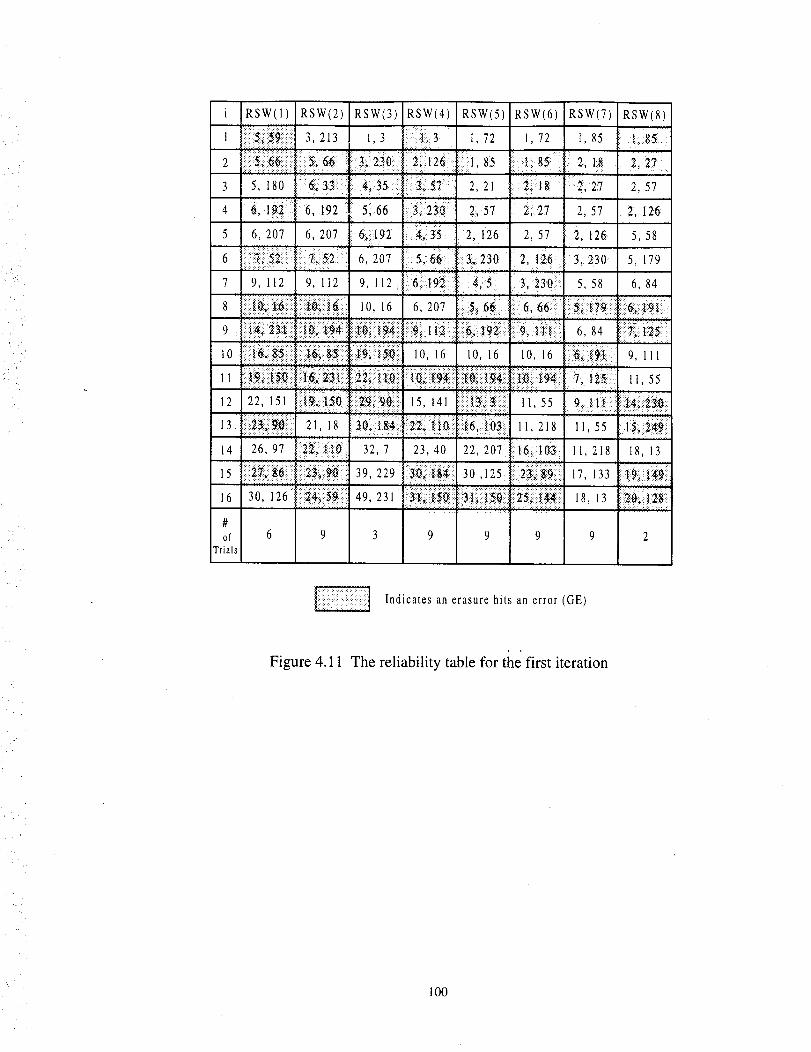
ii?::
i RSW(I) RSW(2) RSW(3) RSW(4) RSW(5) RSW(6) RSW(7) RSW(8)..... >.
1 iiii:::_ii::ii_iiiiii3, 213 1, 3 3 1, 72 1, 72 I, 85 i i1; _:
3 5, 180 2, 21 2;] :: _ 27 2, 57i; :i:i ; ,;,,;;, : ::.-: , J:iii
4 :_, 1_2 L92 | 5;.66 2, 57 2; 27 2, 57 2, I26:: : :_ m,] iiiii [[
• ..: ..
5 6,207 6,207 6_i!t92 , _,:35._ 2, 126 2, 57 2, 126 5, 58::,i • , (,
!:!. :::!:!:!: ::::::::2;
..............."_ ...... _ 3_ 230 2, 1: 3, 230 5, 1796 _:::_:_:5:_ _: 6,207 5,6_ 26:
9, 112 9, 112 9, 112 : , : : [ 3,23_ 5,58 6, 847
8 ii::::::_i_i_i_::_i::;il 10, 16 6, 207 5_ 6_: 6, 66
9 :::i_i 6 84
] 10 16 10 16 10 16 9, 11110
if::! :i::ii _i:i::::_i:;? :, iii::i ::::::::::::::::::::::::!!iii::il;::iiiii!i::i_:::_i::iii!"
12 22, 151 i::_:ii_:]l:50!_:_:.i_:_ii_i; 15, 141 ::::::::" "::::::::::::::::::::::::::::::: 11, 55 %":::: :': "1'::':;,; ;:;;;: ;:;:;:;:;:;:;'| 1:::::::5:::::: :::; :::;:::::::: ; ; ::: : :::::::::::::::::::::::::::
13 ::::::::::::::::::::::::21, 18 3t_:_:_; i:i:.[:6,_0_ 11, 218 ' 11, 55 [ l_i;:_i_ii_ii
14 26, 97 32,7 23, 40 22, 207 1::i[6:t0_ : 11,218 t8, 13
15 i::?ii271_i_}:ii::i2N:::i_ : 39, 229 )3i_)l_N)30 125 ::.....2::_::::8:_:_::":::::::...... 17, t33 ;:ii_;; i_i_:::: ::::::: ::: ::::: ::::::::::::::::::::: ' _:i:: ::: ::
16 30, 126 i_:::i_i::_i::::il49, 231 i_iiii i:_:i: i::3ii_:iiiSi_i:i":.............._:::::::::_i::i2N_it:N_i::i::18, 13 :::._::_;i;Z_::::::::::::.:::::!:i::!i:: :: :: : :::::: :!: : ::::'::"::::::: : :::, :::::i::i:i::i::i:: _t:i:i:i/,i; :,.::: -..:
#of 6 9 3 9 9 9 9 2
Trials
Indicates an erasure hits an error (GE)
Figure 4.11 The reliability table for tile first iteration
100
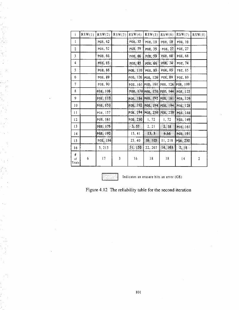
:i ¸ .
i RSW(I)
1
2
3
4
5
6
7
8
9
10
11
12
13
14
15
16
#
of
Trials
RSW(2) RSW(3) RSW(4) RSW(5) RSW(6) RSW(7)
^ GE, 1 i
PGE, 52 !P!G_ _,59 :!:t_GL 3_ PGE, _: :PGE, 27::: ::5:::: • ::::: :x.: :::::::::¢.:
I:PGE, 66 PGE, 6_:.:: PGE, 68' :::: :: i:::: :i:::: :::5 :ii::,:::5: ::.::::,::::::5:: :::::::: ::::::: :
i:!:!:i::i:!::;: :;?!i fi:i: ::.i::::i.:i:i :i:i :? i: ii ::i :' i
POE_:_I(_ I_GE, 8::5 iPGE;:851 PBE, 85......, i :!::::: :;? :!! :: ..... :iii:FGE, S9 'POE;: _26 FGE; 126_i PGE_ PGE, 89
i:i i. _:i.i i:i f:: : ;
PGE, 90 PGE, i6i i PG_i PGE, 126 _,:':109
:i:iii: ........ '[_ iii J ._Siiiii_:
...........= ......................... : .............................::.....................::=:::::i:i:iT:i:;i:i::i:,i:::i:i:i:=i:
;::_" :: _:_::'_ :::::::.:.: :::. :. : _:::::::::: : :,
• i?_: !'!_ :! !'!'?
:::: :::::::u:: :. ::::::::::::::::::::::::::::::::::::::::::::::::.... _:: ::::::::::::::::::::::::::
_G_iii_ 23, 40 i::_i_i::::_::_ii 11, 218 _!:._::i:i:i :h:,:,: ............ :=::::.= .......................
....... x. ;;; :..:
3, 213 . ::_;{i!i]_i_iii 22, 207 !_:_._i_i_::_:::_l_:;_:'i_ :::ii:_:._:................................................,.:........ ,: .,:.::,:. :::.: ,., ::.: .:::.:.: .:. :_
I
6 17 [ 3 16 18 18 14
I
Indicates an erasure hits an error (GE)
RSW(8)
Figure 4.12 The reliability table for the second iteration
101
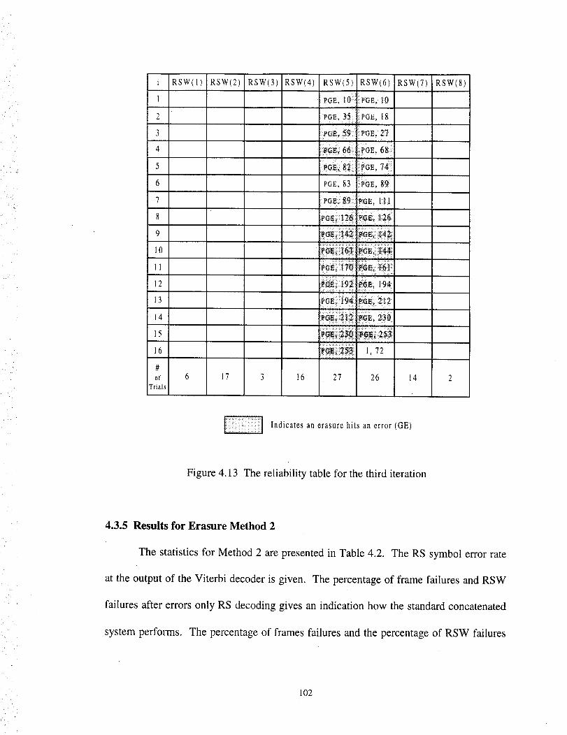
i RSW(I) RSW(2) RSW(3) RSW(4) RSW(5) RSW(6) RSW(7) RSW(8)
1 PGE, lO PGE; 10
:{:
2 PGE iPGE, 18!' _1::
3 PG_, :_9:::, PGE, 27
4 :i_Eii 66 POE, 68_
5 E, 74: 5::
6 PGE, 83 lieGE, 8_:: i I
7 PGE;::89:I P6E, 1it
8 PGE_ li2_:. _GE;: 1_6
: :: :: : : :!:?: :.. :.: :.:
......
_0
+ ' i!_! !:!|,_!: _ , i
................. :::::
16 _.i_:_: 1,72
#of 6 17 3 16 27 26 14 2
Trials
Indicates an erasure hits an error (GE)
Figure 4.13 The reliability table for the third iteration
4.3.5 Results for Erasure Method 2
The statistics for Method 2 are presented in Table 4.2. The RS symbol error rate
at the output of the Viterbi decoder is given. The percentage of frame failures and RSW
failures after errors only RS decoding gives an indication how the standard concatenated
system performs. The percentage of frames failures and the percentage of RSW failures
102
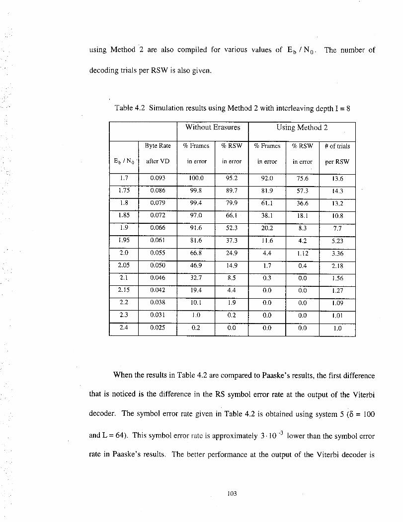
using Method 2 are also compiled for various valuesof Eb /N 0.
decoding trials per RSW is also given.
The number of
Table 4.2 Simulation results using Method 2 with interleaving depth I = 8
Without Erasures Using Method 2
E b / N O ,
1.7
1.75
1.8
1.85
1.9
1.95
2.0
2.05
2.1
2.15
2.2
2.3
2.4
Byte Rate
after VD
0.093
0.086
0.079
0.072
0.066
0.061
0.055
0.050
0.046
0.042
0.038
0.031
0.025
% Frames
in error
100.0
99.8
99.4
97.0
91.6
81.6
66.8
46.9
32.7
19.4
10. I
1.0
0.2
% RSW
in error
95.2
89.7
79.9
66.1
52.3
37.3
24.9
14.9
8.5
4.4
1.9
0.2
0.0
% Frames
in error
92.0
81.9
61.1
38.1
20.2
11.6
4.4
1.7
0.3
0.0
0.0
0.0
0.0
% RSW
in error
75.6
57.3
36.6
18.1
8.3
4.2
1.12
0.4
0.0
0.0
0.0
0.0
0.0
# of trials
per RSW
13.6
14.3
13.2
10.8
7.7
5.23
3.36
2.18
1.56
1.27
1.09
1.01
1.0
When the results in Table 4.2 are compared to Paaske's results, the first difference
that is noticed is the difference in the RS symbol error rate at the output of the Viterbi
decoder. The symbol error rate given in Table 4.2 is obtained using system 5 (8 = 100
and L = 64). This symbol error rate is approximately 3- 10 -3 lower than the symbol error
rate in Paaske's results. The better performance at the output of the Viterbi decoder is
103
most likely due to the increased soft decision levels (L = 64) as compared to the 8 level
soft decision used by Paaske. This slightly smaller RS symbol error rate translates into
slightly better results for the errors only decoding. The frame error rate and RSW error
rate in Table 4.2 are typically 2% or 3% smaller than the results that Paaske obtained.
The results obtained using Method 2 are better than Paaske's results in three
regards. The percentage of RSWs and frames in error is lower. For example, at E b / N O
- 1.9 dB, the percentage of frames and RSWs in error using Paaske's method are 26.8%
and 16.3%, compared to 20.2% and 8.3% using Method 2. Method 2 also obtains these
results using considerably less decoding trials. Paaske's method requires an average of
112.4 decoding trials per RSW to obtain the reduction. Method 2 requires an average of
7.7 decoding trials per RSW.
improvement for lower values
The third improvement is in the ability to obtain
of E b/N 0. The results in [7] indicate that no
improvement is obtained at E b / NO= 1.8 dB. Using Method 2, the percentage of frames
in error was reduced from 99.4% to 61.1% and the percentage of RSW in error was
reduced from 79.9% to 36.6%. The average number of decoding trials per RSW needed
to accomplish this is 13.2. Error reductions were obtained for values of E b / N O as low
as 1.7 dB. Both Method 2 and Paaske's method obtained 0.3 dB gain over the system
using no erasures.
The reduction in average number of RSW trials as compared to Paaske's method
can be attributed to the ability to use erasures in the first decoding attempt. This is useful
for decoding RSW that contain more than 16 errors, as in the example in Figure 4.10.
Each RSW in the frame contains more than 16 errors. Paaske's method would obtain no
104
successful decoding in the first iteration, and would have to resort to using EP4 to obtain
the first successful decoding. EP4 randomly erases two symbols and attempts decoding.
This repeats until a successful decoding or this has been attempted Tma x times. It can
easily be seen that this frame would require a large amount of decoding trials. In
addition, Paaske's method requires two successfully decoded RSW with errors in the
identical positions in order to use EP 1. Erasures declared using EP1 have a probability of
0.96 of being a GE. If not, a less reliable procedure must be used (EP2-EP4). Erasure
Method 2 only requires 1 RSW to be able to declare erasures with a probability of 0.93 of
being a GE. It can be seen that erasure Method 2 converges on the erasures quicker than
Paaske's method, and thus, requires less decoding trials per RSW.
4.4 Erasure Method 3
Method 2 can be modified to reduce the number of decoding trials per RSW by
making a few observations. In Method 1, erasures were erased two at a time until either a
decoding success was obtained, or a maximum number of erasures were declared. This
was done because symbols with low reliabilities were not guaranteed to be GE. Erasing
more than two at a time may cause the decoding capability of the code to be decreased.
This occurs if the number of BE is greater than the number of GE. In Method 2, when a
PGE is declared, it is highly probable that this is a GE (0.93). Instead of erasing two
symbols from the RT at a time, all symbols flagged as PGE are automatically erased. If,
after decoding with these symbols erased it is still not successful, then two more symbols
are erased until the maximum allowable erasures is reached.
105
A second modification updates the flags after a RSW has been decoded correctly,
rather than after all of the RSW in the frame have been attempted. This allows for the
possibility for the highly reliable PGE to be declared in the first decoding pass. Both of
these modifications reduce the average number of RS decoding trials when compared to
Method 2, with very little effect on the performance. The procedure can best be
demonstrated with an example.
4.4.1 An example of erasure decoding using Erasure Method 3
Consider the deinterleaving frame in Figure 4.10. The reliability table before the
first decoding attempt is given in Figure 4.11. Much like Method 2, decoding of RSW(1)
is first attempted using erasure Method 1 (i.e. decoding is attempted using no erasures,
and decoding is repeated until either a successful decoding or a maximum number of
erasures has been reached). RSW(1) is finally decoded after 6 decoding trials and 10
erasures. In Method 2, the next step would be to attempt decoding of RSW(2) using
Method 1. Method 3 instead updates the flags immediately after RSW(1) has been
successfully decoded. This results in 13 PGE being declared in RSW(2), 12 of which are
GE. This modified reliability table is given in Figure 4.14. At this point, RSW(2) is
ready to be decoded. Instead of erasing two symbols at a time as with Method 2, all PGE
are erased and decoding is attempted. For RSW(2), this still does not yield a successful
decoding, but as can be seen from Figure 4.14, erasing two at a time would achieve the
same results, but with more decoding trials. Because the number of PGE are less than the
maximum number of erasures allowed, two more symbols are erased, and decoding is
106
iii_)i_i"_
¸4¸¸¸
/ 'L '
'_L• •
!k •
• i!ii!!__
attempted. RSW(2) finally decodes once 16 erasures have been declared. This is
accomplished in 3 decoding trials, as compared the 17 trials needed to decode RSW(2)
using Method 2. The flags are now updated using the information provided by RSW(2),
and the resulting reliability table is given in Figure 4.15. The flags declared from
RSW(1) and RSW(2) yield 10 PGEs in RSW(3), 8 of which are GE. It should also be
noted that the PBE that were declared removed potential BE from the table. Symbols at
positions 207 and 112 would have been included in the reliability table. These would
have resulted in BE if used. The decoding of RSW(3) is accomplished by erasing the 10
PGE in the table. This resulted in a decoding success in only 1 decoding trial. The flags
are modified using the information provided by RSW(3), and the resulting reliability table
is given in Figure 4.16. There are 11 PGE in RSW(4), and all are GE. This RSW
requires all 16 erasures for a successful decoding, and is accomplished with 4 decoding
trials. The flags are updated and the resulting reliability table is shown in Figure 4.17.
There are 15 PGE in RSW(5) and 14 are GE. The codeword contains 23 errors, and
cannot be decoded with the 16 erasures in the table. This codeword will require 15 out of
16 erasures to be GE for a decoding success. Two decoding trials were attempted on this
codeword. Decoding of RSW(6) is attempted by declaring erasures at the positions where
the 9 PGE have been flagged. This does not yield a successful decoding, so erasures are
declared 2 at a time until the maximum is reached, at which point a decoding success has
not been obtained. This required 5 decoding trials. RSW(7) is successfully decoded by
erasing all 12 positions with PGE flags, and decoding. RSW(7) required only 1 decoding
trial to decode successfully. The flags are updated, and the resulting reliability table is
107
given in Figure 4.18. RSW(8) contains 16 PGE, and 13 are GE. There are only 17 errors
in RSW(7), and is easily decoded in one trial by declaring 16 erasures. The flags are once
again updated and the resulting reliability table is given in Figure 4.19. Decoding of
RSW(5) is attempted a second time. New information has been provided by RSW(7) and
RSW(8). There are 17 PGE in RSW(5), and all are erased in the first decoding attempt.
In Method 3, more than 16 erasures can be declared if all are PGE. RSW(5) successfully
decodes and the updated reliability table is given in Figure 4.20. RSW(6) has 20 PGE,
with 19 of these being GE. All 20 symbols are erased, and the word is successfully
decoded. The total number of trials for this frame is 25, which corresponds to an average
number of trials per RSW of 3.13. This is significantly less than the number of trials
required for erasure Method 2 to decode the same frame. The results of the simulation are
given in Table 4.3. It can be seen from the table that a gain of 0.25 dB is obtainable.
108
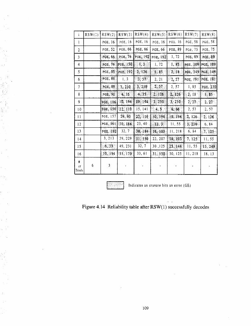
:.i
iili
2
3
4
5
6
7
8
9
10
11
12
13
14
15
16
#of
Trials
RSW(I) RSW(2) RSW(3) RSW(4) RSW(5) RSW(6) RSW(7) RSW(8)
PGE, 16 PGE, t6 PGE, 16 PGE, 16 PGE, 16 PGE, 58 PGE, 58
PGE, 52 PGE, 66 i _E, 66 PGE, 66 PGE, 89 PGE, 75 PGE, 75
.... ii
:::: ..:::: ::::.::...:::::::-: .-....... ::: ::x x::: ::::.::-: ::::
::_GE; _6 1, 3 i:i_i 57ii!i::i 2, 21 i:.::_2_:27 ::::_t_i, t:91: r'_I_::, l_::t:.
i:_ii ::i_ 3;_i_. i :i_!12121_:: _: ::: i:::: :[_E, : : ::i:I
l:.::._:_:"_:i:i:i!i ::::::::::::::::::::::::::::::::::::::::::::::::::::::::::::::::::::.:::::.=:i::.:.:i:::.:.:.:.:::..........................:........... .... _.:i?_!._.i:_:i!:i!ipG_i!_6! i_i:_ii3_i'_i !ii!_!i_51ii! i 2!_iii2_ii !i_!_::i_:_i_ .... 2= t8 .................. ":: : : :::::: ::: : _::.:: : ::::::::: :::: :::::::::_::::::::::::.::::::::: ::::::::::::::::::::::::::::::::::::::::::::::::::::::::::::::::::: ::: t_ :_::::: :_:_:x:., i : _i.ii:_
: _ I0_: t_i _94::i ::Iitl_!:i11_);_:i:-:i:!_ii::_310_:i!i _i_:_230:i:ii 21ii:27: 2 _:i::ii: : :-?: !:!:?][:!: i?:?:?:?i:i:i: 37:::::::
15, 141 i::::i:_i_i_::.i :: _i:i:-_/ : 2, 57 2, 57
::$: :::::5: :::::5:: : .: ::.:::::5::: :: :::::::::::::::::::::: ::::::::::::::::::::: :::::::::::::::::::::: : ::::
POE 157 i 2_i:e_l) [::::_ii [il_ :::::::::::::::::::::::::::i::l_:, i::_9_iii 126: _:21:
GK.:[_I:: ii:30::|iiS_ii:: 23 40 :.::i:::t_3¢31::::I 11 55 i::31;::i_:It_..... 6, 84...... ::: :i: :: :::: : :5 :5::
:P_,:i_::_i; 32, 7 ii;_iiiS_::_: 11, 218 6, 84 :::_i l_i_Si::_:i
3,213 39,229 !ii:_iii_:ii1_ ' 22,207 ::':_:}[i_,iiii_!i_: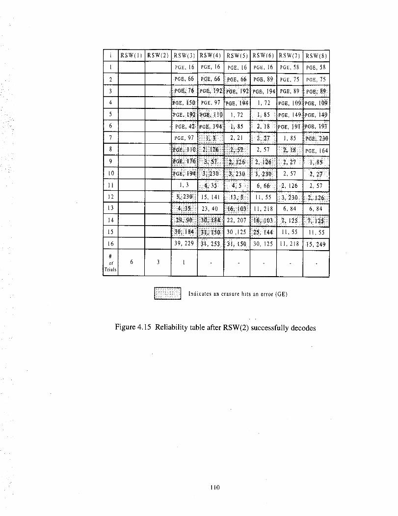
i _,
:i
iYi ,
i
1
2
3
4
5
6
7
8
9
10
11
12
13
14
15
16
#of
Trials
RSW(1)
6
RSW(2) RSW(3) RSW(4) RSW(5) RSW(6) RSW(7) RSW(8)
PGE, 16 PGE, 16 PGE, 16 PGE, 16 PGE, 58 PGE, 58
PGE, 66 P_E, 66 _GE, 66 PGE, 89:: PGE, 75 PGE, 75
IPGE::;i7_i : .... "_...... _:' PGE, 89' _PGE;:i9z P_E_i 19:_ PGE, 194 PG_ 18_
_GE, _. PGE, 97 P'GE, 1:_ 7 I, 72 aGE, 109 PGE, l_i
_GE,ii Ii_71!i_i_; 1 li_'! 1, 72 I:, 85 PGE, 149] PGE,: i_!""ga
Pc;z, 4_: _I'GiE,194 L 85 2, t8 POE, ic_ "PGE, _9_:
• . :xPGE, 97 2, 21 :: 2.._ 1, 85 :P+6_, 2:a+0.............................ii:i!ii:ii.iiiiiii.:..............................:.. ...L:, ,...;......... ::"_1_ 1 l::t}iliii!i:2iiiiii!ii2_ii!ii 2, 57 PGE, 164
:.: ::.: ,:::.: :k::::: :::::::::: ::::::
l +I++:: +++++++++:++:+++:+++++:+++++.+:+++/:+:+Y+:?:+++:++++++:+::::::+::?:+:?,+;:+."+,+;+::+:.++i++:++++++++ :+:++y+
+++_+++_3'+}++(:++_i_23_ + ++++i++2+3++++2, 2, 27:Gt_::;i:19_+1::i , 57:+::_: i:i:+l::+::!::: _:li!_ii!::ii: :i. .... ....... .....;1,3 3+" _i5 6','16_i 'i2, t26 2, 57
::: ::::: :: : :_:::: . : ::;:!
23: 15, 141 11 55 ::::3;:23_:..... •: ;;; ; ,;;:;,,.;.' _ !:i:::_ -: ::_:i_::.: -:.::::i::::: ?::::: :?::::::: ...:::.:::.::: :::::::
23, 40 ::_i_ii+li_ 11, 218 6, 84 6, 84.+H :..:.:. :::.:::.::: ::::.:::+ ::::: :... :
::::::::::::::::::::::::::::::::::::::::::::::::::::::::::::::::::::::: ::t: :: : :.:::.:.:: " :.._. :.:.::.:.::.
_9_ _::::::ii::_ii_i!_::_i:_:22, 207 :::_!_iil03: : 7; 125+..... • :::::::::::::::::::::::::::::: : :::::: : +:" ::_:: : ii i_:+:
I 3e; I:::8:+::++2m+]:;:+l+_++++30 ,125 '::_; t4_ 11 55 11, 55i:i ::.... ::ii i:ii:i:i:.i::::>;. :.: -.::,.i. ,, ': +:
39, 229 ii3ii,253 3i+ IS+J: 30, 125 tl,218 -I5,;.49
3 1
!I Indicates an erasure hits an error (GE)
Figure 4.15 Reliability table after RSW(2) successfully decodes
11o
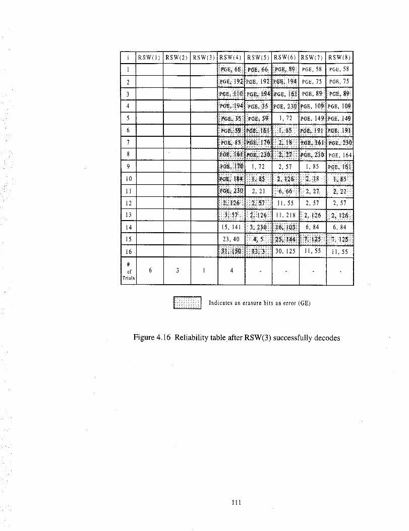
i RSW(1)RSW(2)RSW(3)1
2
34
5
6
7
8
9
10
11
1213
14
15
16
#of 6 3 1
Trials
RSW(4) RSW(5) RSW(6) RSW(7) RSW(8)
::gGl_ 192i :.PCE 192 ::P_E;t9_ POE, 75 PGE, 75
!_l'e_, _::9ti[ii,a::E,)_5:]iPOE, 23_iii_OE 10_:: PGE, l
i:::.i_6_:85i:.::ii_i::, t7/_i::::::::::::::::::::::::::::::::::i::i:i:::::i:i: .:.:. i:i :i:i:i::i:i:i:; :?: :i:i::i:i: ::::::::::::::::::::::::::::::::: :ii:: :? iii :: :|::: :;:_
..... :::::::::::::::::::::::::::::::::::::::::::::::::::::::::::::::::::: :: !::! |
_i:?:: : ::i::;?i :i:i::i.: i:i: :::i: :: i_ ::::::::::::::::::::::::: :: _f,::!.: : :::::::::::::::::::::::::::::::::::::::::
i::: _::i:!:! :::::::::::::::::::::::: i::i :i:|i:: -: i::::9:::?[ ::i :: :: : :::?::
:i:i :ii:i:i:::i )i:i :;i:i:; :_ii i :::::i :::: , " ::: ::
...... : :":: : ::::: m:. .:.: : :.:.:.: :..:: < : :.:.: :.: :.: .:.:. :.: # ' :::::
i::i!_::ii::iS_:_i::i_i!i12'61::: 11 218 i::ii2,_26 _:_::_:_fi:::.............. ::,t_ :::::::::::::::::::::::::::: :::: :::::::5:::
15, 141 i:::::3; 2_¢Jii_:::ii::i:_:_!i::_!ii:_!_6, 84 6, 84..... ::: :::::::::::::::::::::-.:: :: :: :.:i:: :. ::_.: : :: _:::::::
23, 40 ::iiii:_i_5 ::::i[::ili_ii::iii_i::i::i[i:::.::i::_i:::::_i_i_....... !:: i::.:: iiii:| _!i:i :i:i::i:iiii iii _iil)i:iiii:ii?: :: • .:. ::::::
===========================================================================
Indicates an erasure hits an error (GE)
Figure 4.16 Reliability table after RSW(3) successfully decodes
111

Eli
sapoaop ,qlnjssoaans (_)A_S_I aolje Olqm fil!l!qe!lO_I LI "# oJng!.q
(39) JOJJg U_ Sl!q OJnSgJO fig SOleo!pu I
1 1 E 'e I _ 9
';I d ......::" 'III 9 _Z:l-::::a_ _L I _8 'aga
• . , ::_::_ :: :. • .:::_: ::_,,:,_:::_k ::
a,, i:::: I 6_ '_aii1 i
_fJl '_Od :601 "_Od O_E ,abel _ '_to_
:68'/I9d 68'_I9d _9I 'idOd:ii_6_:"ad9_l:55 :"
tL '_]gd 1L '_Od 1'6I ;:JOd_{'{:g61'EOaZ(Y
•_. H,
(8)A_S_I (L)h_S8 (9)ACS_I (!)A_S8 (I)A_S_I
Sle!.LLjo#
9I
fl
'el
1I
Ol
6
8
L
9
f
'e
I
1

_II
sopooop ,qlnjssooons (L)AkS_I aolje olqel ,(l!I!qe!IO_I 81 "17oang!_I
(39) aolao u_ sl!q o_nsr3o u_ sol¢o!puI
I I g E _ I [ 9
6LI 'aDd _;L '1 _::giL'i:'_
*:::': • ::i:i !: : :1:: : i:
............... :ii i i :
• iiliy, ,:.
..... tr
II1 '_IOd i_gl '_lOd Ogg _aOd. .i :r
_9:1 ,_tod gel _aod 0_i :i_gd
OgZ '_o,!: il I !aod" _jg 'ag,_),i . .i i : i.
_;:i_ ::r il :::: : ::::: _
i
68 '_gd 68_:aOd 99 'aOd
(_)_S_I ([)_S_I (_)_S_ (1)A_S_I
ste!.LLjo#
9I
"17I
II
Ol
6
8
L
9
I
1
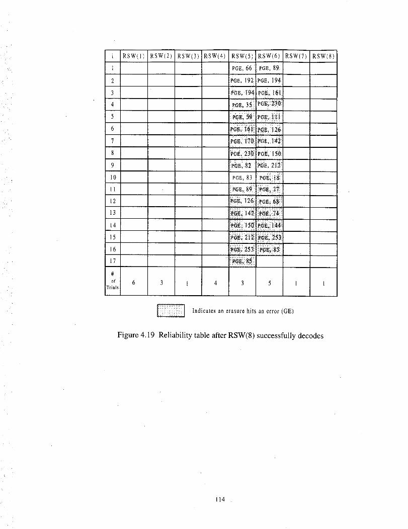
i RSW(1) RSW(2) RSW(3)
1
2
3
4
5
6
7
8
9
10
11
12
13
14
15
16
17
#
of 6 3 ITrials
RSW(4) RSW(5) RSW(6) RSW(7) RSW(8)
PGE, 66 VGE, 89_: ill
_E, 192,pGE, 19_,) i i , i . :. .:: :
r_E, I94 PGi_i 1_t::
...._.. ....
_G_, 83 ea_{i}*::
_]];];d;i, _??_ _ i < "
,:ili
• - : -':::::::::::. ::::: :
4 3 5 1 1
Indicates an erasure hits an error (GE)
Figure 4.19 Reliability table after RSW(8) successfully decodes
114
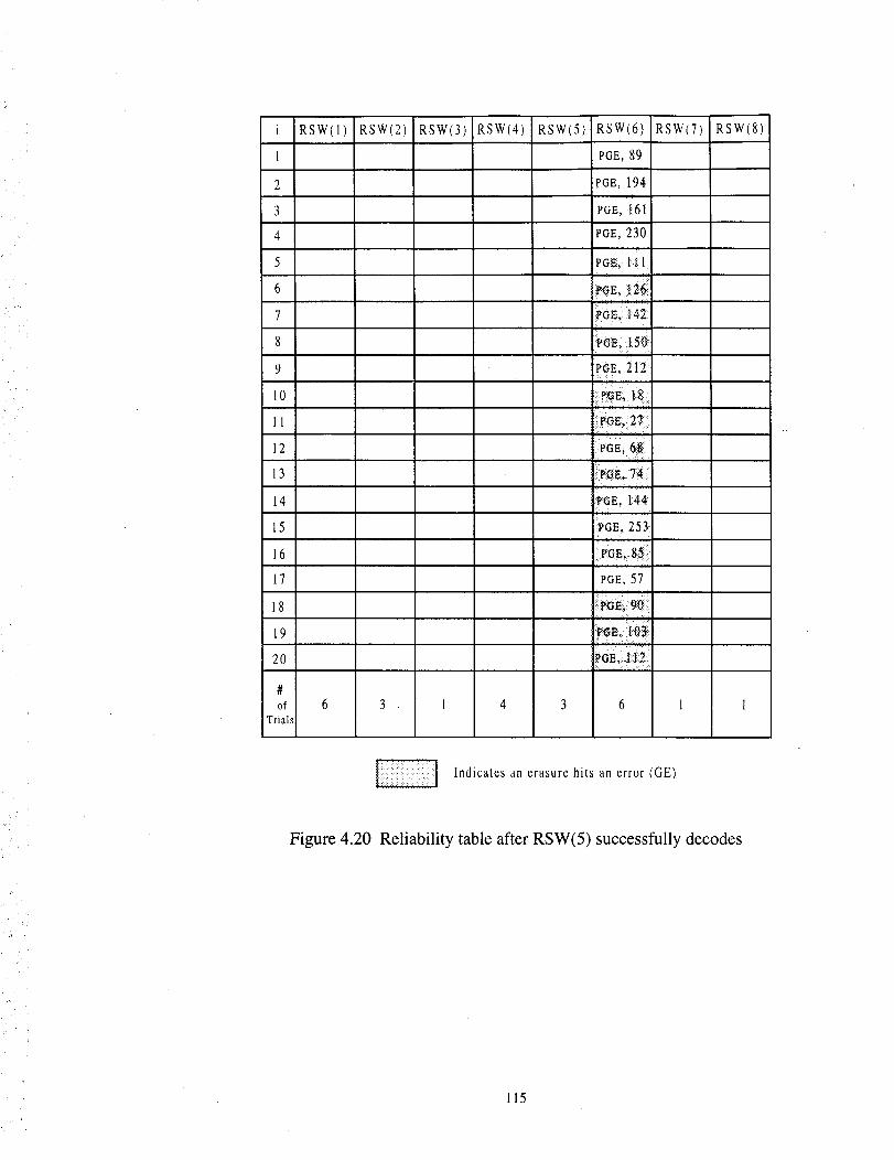
i RSW(I)
I
2
3
4
5
6
7
8
9
l0
11
12
13
14
15
16
17
18
19
20
#
of
Trials
RSW(2) RSW(3) RSW(4) RSW(5) RSW(6)
PGE, 89
PGE, 194i
PGE, I61
PGE, 230
PG_, 1:{ 1
PGE,: :[4_
f_e; ilSe:
r'_E, 2
:PoE 68:iii
;_aE, 253
PaE, 57
i i,i _hi?
GEi::112
RSW(7)
6 3 1 4 3 6 1 1
RSW(8)
Figure 4.20
Indicates an erasure hits an error (GE)
Reliability table after RSW(5) successfully decodes
115
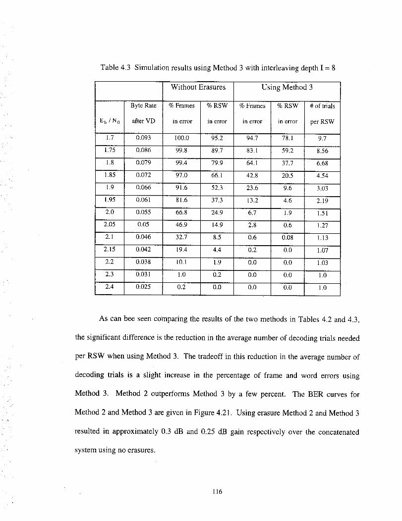
Table 4.3 Simulation results using Method 3 with interleaving depth I = 8
E b / N O
1.7
1.75
Byte Rate
after VD
0.093
0.086
Without Erasures Using Method 3
% Frames
in error
94.7
83.1
% RSW
in error
78.1
% Frames % RSW
in error in error
100.0 95.2
99.8 89.7
99.4 79.9
97.O 66.1
91.6 52.3
81.6 37.3
66.8 24.9
46.9 14.9
32.7 8.5
19.4 4.4
10.1 1.9
1.0 0.2
0.2 0.0
59.2
# of trials
per RSW
9.7
8.56
1.8 0.079 64.1 37.7 6.68
1.85 0.072 42.8 20.5 4.54
1.9 0.066 23.6 9.6 3.03
1.95 0.061 13.2 4.6 2.19
2.0 0.055 6.7 1.9 1.51
2.05 0.05 2.8 0.6 1.27
2.1 0.046 0.6 0.08 1.13
2.15 0.042 0.2 0.0 1.07
0.038
0.031
2.2 0.0 0.0 1.03
0.0 0.0 1.02.3
2.4 0.025 0.0 0.0 1.0
As can bee seen comparing the results of the two methods in Tables 4.2 and 4.3,
the significant difference is the reduction in the average number of decoding trials needed
per RSW when using Method 3. The tradeoff in this reduction in the average number of
decoding trials is a slight increase in the percentage of frame and word errors using
Method 3. Method 2 outperforms Method 3 by a few percent. The BER curves for
Method 2 and Method 3 are given in Figure 4.21. Using erasure Method 2 and Method 3
resulted in approximately 0.3 dB and 0.25 dB gain respectively over the concatenated
system using no erasures.
116
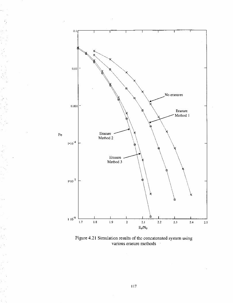
0.1
Noerasures
Erasure
Pe
I" 10 -4
1"10 5
ErasureMethod 2
Erasure
Method 3
\\
\
\
1 10-6 I I I I t_ I I I
1.7 1.8 1.9 2 2.1 2.2 2.3 2.4
EdNo
Figure 4.21 Simulation results of the concatenated system using
various erasure methods
2.5
117
ir
Chapter 5
Conclusions
Performance of the concatenated coding system through the use of RS symbol
erasures has been demonstrated. The first method investigated uses reliability
information generated by a modified Viterbi decoder. This information is derived from
the metric difference of two paths merging in each state. The reliability for the bits along
the surviving path are updated using this metric difference. This method yielded about a
0.1 dB improvement over the concatenated system using no erasures. This gain was
independent of the truncation length, interleaving depth, and number of soft decision
levels.
In the second method proposed, the reliability table is refined using information
provided by the decoded RSW in the deinterleaving 'frame. The error positions are
known in the decoded word, and the method searches for equal reliabilities in
neighboring, non-decoded RSW. If the reliabilities are the same, then symbols are
erased. This method yielded approximately 0.3 dB gain over the standard concatenated
system. The average number of decoding trials per RSW is substantially less than the
results presented by Paaske [7]. Using Method 3, the number of trials per RSW is
reduced even further. In addition, Methods 2 and 3 perform reasonably well at very low
118
values of Eb/No (i.e. < 1.9 dB). The cost is the increased complexity of having to use the
SOVA in place of the standard Viterbi decoder.
It has been shown that the use of convolutional code as the inner code and a Reed
Solomon code as the outer code provide considerable gains. The rate 1/2 K = 7
convolutional code concatenated with a (255, 223) t = 16 error correcting Reed Solomon
code yielded about 8 dB gain over uncoded BPSK and approximately 9 dB with an
interleaving depth of ! = 8. The use of an interleaver with depth I = 8 gives a gain of
approximately 0.5 dB as compared to the same system using no interleaver. It has been
demonstrated that the use of a real system results in approximately a 0.3 dB loss when
compared to the ideal system using the same truncation length and number of soft
decision levels. It has been shown that a 0.15 dB improvement can be obtained by
increasing the number of soft decisions used from L = 8 to L = 64. A gain of 0.2 dB is
attainable if the truncation length in the Viterbi decoder is increased from 5 = 32 to 8 =
100. These gains were obtained regardless of the interleaving depth used.
5.1 Future Research
Erasure method 1 declares RS symbol erasures by using reliability information
provided by the SOVA. This method could be improved by using the maximum a
posterori (MAP) algorithm in place of the SOVA. The MAP algorithm is an alternate
method for decoding convolutional codes. The Viterbi decoder finds the maximum a
posterori probability for the entire path through the trellis. The MAP algorithm, on the
other hand, finds the maximum a posterori probability for each outgoing bit. The MAP
119
Algorithm was designed to minimize the word error probability rather than the sequence
error probability as the Viterbi algorithm does. This algorithm is more complex than the
Viterbi, but easily provides log-likelihood (reliability) values at its output. The reliability
values generated by the MAP algorithm yield superior results when compared to the
SOVA, but is very complex. The Map algorithm could be used in place of the SOVA in
the concatenated coding system presented here.
The performance of Method 2 could also be improved upon. The special case
where GE are flagged BE, and vise versa, might be able to be detected and solved.
Several methods were tried unsuccessfully to fix the problem. Performance
improvements could be obtained by incorporating some of the elements used in Paaske's
method, such as EP1, EP3, and EP4. In Paaske's method, when the highly reliable
methods (EP1 and EP2) can not decode some of the RSW in the frame, the backup
methods are used to exhaustively try and decode, which results in a high average number
of decoding trials per RSW. But if through the use of this exhaustive search, a previously
undecodable RSW is now correctly decoded, then this RSW can possibly help in the
decoding of other non-decoded RSW in the frame. This is where a large number of
decoding trials may be justifiable. When Methods 2 and 3 fail to decode a frame, there is
no backup method that might provide improvement. The lack of a backup procedure, is
One of the reasons that the number of trials is low compared to Paaske's method. This
lack of a backup procedure is somewhat justified.
systematically guess the positions of the errors.
In Paaske's method, EP4 is used to
This guessing is effective when the
number of errors is not much larger than 18 or 19. For Methods 1 and 2, most RSW with
120

18or 19errorscanbedecodedusingthe initial decodingusingMethod 1. The SOVA
outputprovidesthedecoderwith enoughusefulinformationto decodesomeof the RSW
that Paaske'smethodwould requireEP4to decode.For example,in section4.5, thereis
anexampleRSframedecodedusingMethod2. EveryRSW in the framecontainsmore
than 16errors. If Paaske'smethodwasusedto decodethis frame,thenEP4wouldhave
to be used to obtain the first decodedRSW. Using Method 2, three RSW were
successfullydecodedon the first trial, andthe otherswere successfullydecodedusing
informationprovidedby thesedecodedRSW.
Anotherpossibleimprovementis theuseof iterativedecoding.Iterativedecoding
takesthe outputof theReedSolomondecoderandfeedsthis to the input to the Viterbi
decoder.Paaske[7] usediterative decodingin his paper. If therearestill undecodable
RSW in the deinterleavingframe,the correctedcodewordsaresentback to the input to
the Viterbi decoder.The correctedbits give the Viterbi decodersomeof thestatesthat
the correctpath took. Forcingthe Viterbi decoderthroughtheseknown statesmayhelp
the Viterbi decoderin a betterestimateof thecorrectpath. The error rateat the output
will be reduced,which will result in more RSW being decodedon the secondtrial.
Iterativedecodingcouldbeusedwith Methods2 and3 presentedin this report.Thereis
the potential for larger gains using this repeatedViterbi decodingbecausethe first
iterationwill havecorrectedsomeof theRSW,andprovide thesecondViterbi trial with
additionalinformation. It shouldbenotedthatthis repeatedViterbi decodingis effective
only whentheoutputof theRSdecodercontainssomecorrectlydecodedRSW. Methods
2 and3 allow for a reductionin RSW failure for Eb/No valuesat as low as 1.7dB SNR.
121

Even though the reduction at the very low values of Eb/No is not very large, this little bit
of reduction would help greatly if used in repeated Viterbi decoding trials.
The systems investigated in this report could be simulated using SPW. SPW is a
useful' tool for modeling of communication systems. Many signal processing blocks such
as filters, modulators, and channel models are contained in SPW's library for use in the
design of larger, complex systems. The SOVA and the errors and erasures RS decoder
are currently not in any of the libraries found in SPW. SPW does allow for "custom
coded blocks". This tool can take C code, and create an SPW block based on this code.
This custom coded SPW block can then be used in combination with other SPW blocks
in the design of communication systems.
The SOVA could be implemented in a single chip design. The method presented
by Hagenauer and Hoeher could be used, or another method presented in [2].
122

I
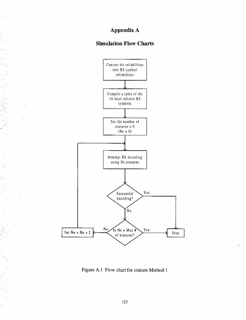
Appendix A
,(
j
Simulation Flow Charts
SetNe=Ne+2
Convert bit reliabilities
into RS symbolreliabilities
Compile a table of the16 least reliable RS
symbols
Set the number of
erasures = 0
(Ne = 0)
iAttempt RS decoding
using Ne erasures
Yes
N°go@ Yes I st
Figure A. 1 Flow chart for erasure Method 1
123
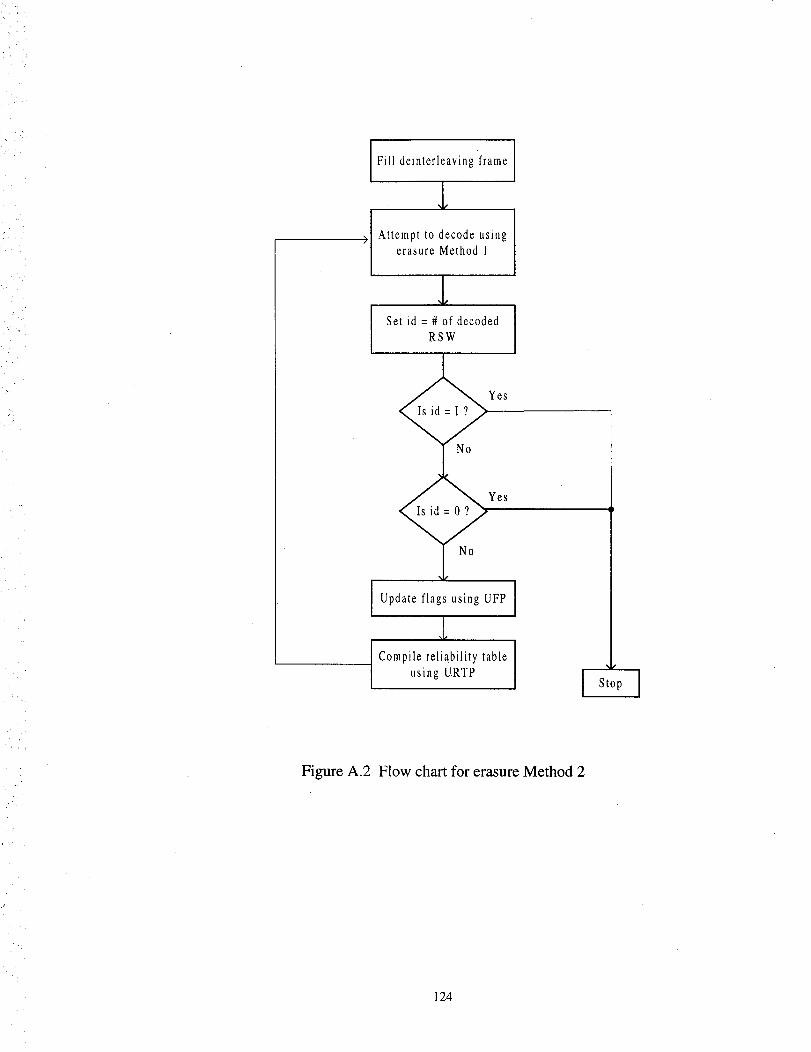
, ,i ¸¸¸
Fill deinterleaving frame
Attempt to decode usingerasure Method 1
I
Set id = # of decoded ]
IRSW
@YeSNN.o °
Update flags using UFP [
,t/
Compile reliability table /
using URTP l Stop
Figure A.2 Flow chart•for erasure Method 2
124
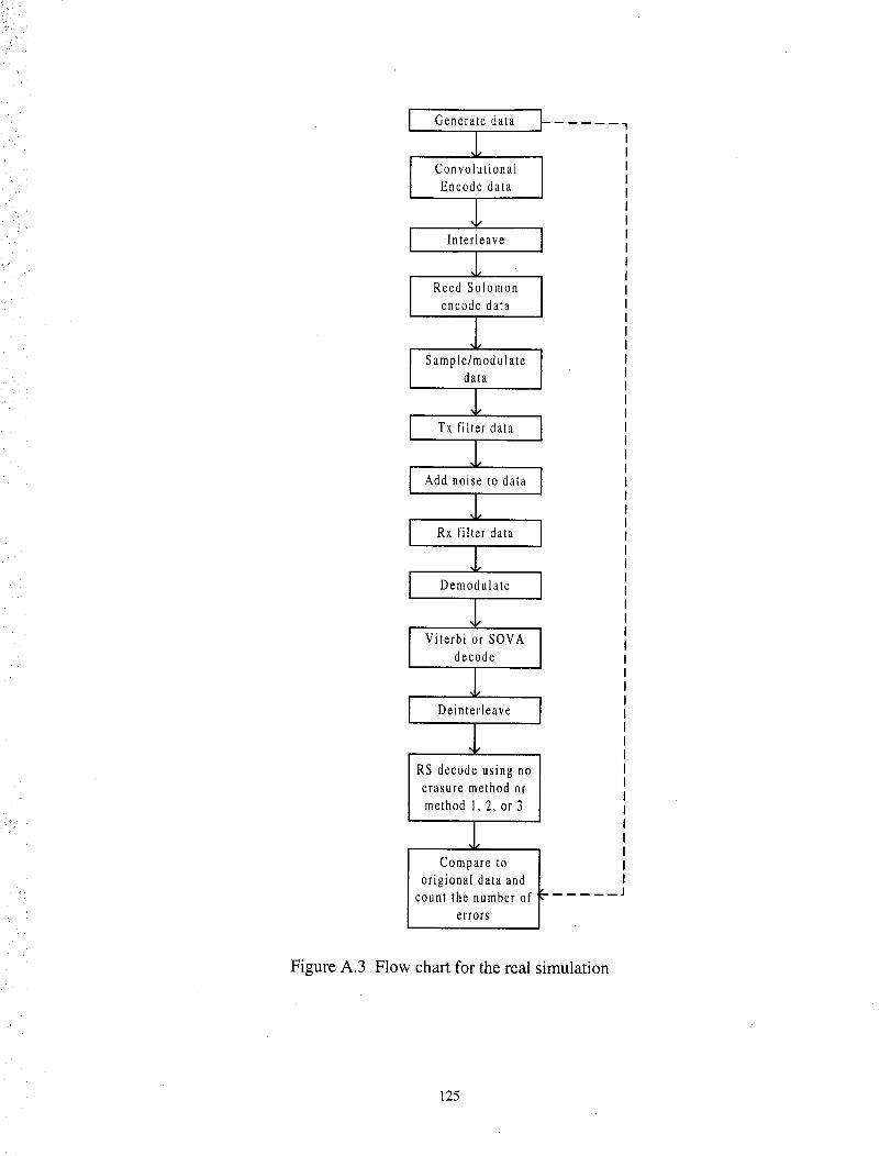
I Generatedata
ConvolutionalEncodedata
1I Inter,eaveI
,LReed Solomon Iencode data
lSample/modulatedata [
,l,I Rxfi,ter,_ataI
,l,I Oemodu,ateI
,L[ Deinterleave[
,LRS decode using noerasure method or
method 1, 2, or 3
,L
Compare to t
origional data andcount the number of
errors
Figure A.3 Flow chart for the real simulation
125
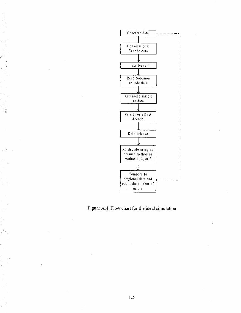
Generatedata I
ConvolutionalIEncodedata
;Interleave [
,LReed Solomon [encode data
Add noise sample [to data I,L
Viterbi or SOVAdecode
Deinterleave
lRS decode using noerasure method or
method 1, 2, or 3
Compare to t"
origional data andcount the number of
errors
_1
Figure A.4 Flow chart for the ideal simulation
126
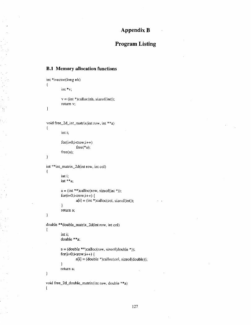
Appendix B
Program Listing
i ¸¸
B.1 Memory allocation functions
int *ivector(long nh){
int *v;
v = (int *)calloc(nh, sizeof(int));return v;
void free 2d int matrix(int row, int **a)
int i;
for(i=O;i<row;i++)
free(*a);free(a);
mt **int_matrix_2d(int row, int cot){
int i;
int **a;
a = (int **)calloc(row, sizeof(int *));
for(i=O;i<row;i++) {
a[i] = (int *)calloc(col, sizeof(int));}return a;
double **double_matrix_2d(int row, int col){
int i;
double **a;
a = (double **)calloc(row, sizeof(double *));
for(i=O;i<row;i++) {
a[i] = (double *)calloc(col, sizeof(double));}return a;
void free 2d double_matrix(int row, double **a)
{
127
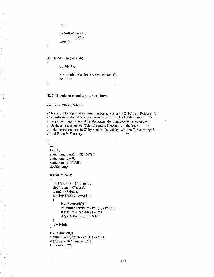
int i;
for(i=O;i<row;i++)free(*a);
free(a);
double*dvector(longnh)
double*v;
v= (double*)calloc(nh,sizeof(double));returnv;
B.2 Random number generators
double ran2(long *idum)
/* Ran2 is a long period randum number generator ( > 2* 10^18). Returns *//* a uniform random deviate between 0.0 and 1.0. Call with idum a */
/* negative integer to initialize; thereafter, do idum between successive */
/* deviates in a sequence. This subroutine is taken from the book */
/* "Numerical recipies in C" by Saul A. Teukolsky, William T. Vetterling, */
/* and Brian P. Flannery. */
int j;
long k;static long idum2 = 123456789;
static long iy = 0;
static long iv[NTAB];double temp;
if (*idum <= 0)
{if (-(*idum) < 1) *idum=l;
else *idum = -(*idum);idum2 = (*idum);
for (j=NTAB+7; j>=0; j--){
k = (*idum)/IQ1;
*idum=IAl*(*idum- k*IQ1) - k*IR1;
if (*idum < 0) *idum += IM 1;
if (j < NTAB) iv[j] = *idum;
}iy = iv[0];
}k = (*idum)/IQ1 ;*idum = IA l*(*idum - k*IQ 1) - k*IR 1;
if (*idum < 0) *idum += IM1;
k = idum2/IQ2;
128
i] ¸ .
idum2 = IA2*(idum2 - k*IQ2) - k*IR2;if (idum2 < 0) idum2 += IM2;
j=iy/NDIV;iy = iv[j] - idum2;
iv[j] = *idum;
if(iy < 1) iy += IMM1;
if ((temp = AM*iy) > RNMX) return RNMX;
else return temp;
float gasdev2(long *idum)
/* This function returns a normally distributed deviate with zero mean and unit variance */
/* This function is more computationally efficient than gasdev I because there are no trig *!/* function calls and the funtion saves the extra deviate for the next funtion call. This */
/* subroutine is taken from the book "Numerical recipies in C" by Saul A. Teukolsky, "1/* William T. Vetterling, and Brian P. Flannery. */
static int iset = 0;
static float gset;float fac, rsq, vl, v2;
if(iset == 0)
{do
{vl = 2.0*ran2(idum) - 1.0;
v2 = 2.0*ran2(idum) - 1.0;
rsq = v 1*v I +v2*v2;
} while (rsq >= 1.0 IIrsq == 0.0);
fac = sqrt(-2.0*log(rsq)/rsq);
/* Now make the Box-Muller transformation to get two normal deviates. *//* Return one and save the other for the next call */
gset = vl*fac;iset = 1;
return v2*fac;
}else
{
/* Set flag */
/* We have an extra deviate handy. Unset the flag and return it */iset = 0;
return gset;
int bitgen(long *idum)
double a;
int bit;
a = ran2(idum);
129
if (a>=0.5)bit = 1;
elsebit =0;
returnbit;}
?!i!
void add_noise(long *idum, double *data, double nn, double sigpow, double EbNo,
double gain){
inti;
double var, sd, A;
A = gain*pow(l 0.0, (EbNo/10.0));
var = sigpow*Nss/(2*A);
sd = sqrt(var);
for (i=0; i<nn; i++)
data[i] += sd*gasdev2(idum);
B.3 Filter
void filter(double *data, int M, double *h, double *x, long nn)[
int i, j;double sum, *x;
x = dvector(2*M+l);
for(i=0; i<=2*M; i++) x[i] = 0.0;
x[2*M-1] = data[0];x[2*M] = data[l];
for(i=2; i<nn+2*M; i++)
{sum = 0.0;
for(j=0; j<2*M; j++){
sum += x[j]*h[j];x[j] = x[j+l];
}x[2*M] = data[i];
data[i-2] = sum;}free(x);
130
B.4 Modulator/Demodulator
void modulate (double *data, int *v, long N)
{
int i, j;
double A;
A = sqrt(2.0*Eb/Tb);
for(i=0;i<N;i++)
{
if(vii]==0){
for(j=0;j<Nss;j++)data[i*Nss + j] = -A;
}else
for(j=0;j<Nss;j++)
data[i*Nss + j] = A;
void demod(double *data, int *out, long N)
{
int i;
double I;
for(i=0;i<N;i++)
{
I = data[i*Nss+Nss/2 -1] + data[i*Nss+Nss/2];
if(I >= 0.0) out[i] = 1;else out[i] = 0;
void demodsoft(double *data, int *out, long N, int **soft_metric, int Q, int a)
int i, j, level, **num_bits_per_level;
double I, b, amp, *prob;
amp = 2.0;
num_bits_per_level = int_matrix_2d(2, Q);
prob = dvector(Q);
131
for(i=O;i<2;i++){
for(j=0; j<Q; j++)
num_bits_per_level[i][j] = 0;
}
for(i=0;i<N;i++)
{I = (data[i*Nss+Nss/2 - 1] + data[i*Nss+Nss/2])/2.0;
for(j=0; j<Q; j++)if(I>=amp*(2*j-Q)/Q && I<= amp*(2*(j+l)-Q)/Q)
level = j;
if( I >= amp) level = Q- 1;
if(I <= -amp) level = 0;
num_bits_per_level[out[i]][level] += l;
out[i] = level;
for(i=0; i<Q; i++)
prob[i] = (double)(num_bits_per_level[0][i] + hum bits_per_level[ 1][Q-i- 1] + 1)/(2*N+Q);
b = -log(prob[Q- 1])/log(2.0);
for(i=O; i<Q; i++)
{soft_metric[O][i] = (int)(floor)(a*(log(prob[i])/log(2.0) + b));soft_metric[ 1][Q-i- 1] = soft_metric[O] [i];
}
free 2d int matrix(2, num_bits_per_level);
free(prob);
B.5 Calculate power
double calc_power(double *data, long nn){
int i;
double sum, P;
sum = 0.0;
for(i=O; i<nn; i++)
sum += pow(data[i], 2);
P = sum/(nn);
132
returnP;}
B.6 Interleaver and deinterleaver
void interleave(int *v, int rows, int rs_n, int rs_m, int I, int num)
{/* rows = rs_m*rs_n, I = interleaving depth */
int ii, i, j, 1, **matrix;
matrix = int_matrix_2d(rows, I);
/* Fill matrix by column */
for (ii=0; ii<num; ii++)
{for(i=0; i< I; i++)
for(j=0; j<rows; j++)
matrix[j][i] = v[ii*rows*I + i'rows +j];
/* Exit matrix by row */
for (i=0; i<rs_n; i++)
for(j=0; j<I; j++)for(l=0; l<rs_m; 1++)
v[ii*rows*I + i*I*rs_m +j*rs_m + 1] = matrix[i*rs_m+l][j];
free 2d int matrix(rows, matrix);
void deinterleave(int *v, int rows, int rs_n, int rs_m, int I, int num){
/* rows = rs_m*rs_n, I = interleaving depth */
int ii, i, j, 1, **matrix;
matrix = int_matrix_2d(rows, I);
/* Fill matrix by row */
for (ii=0; ii<num; ii++){
for (i=0; i<rs_n; i++)
for(j=0; j<I; j++)for(l=0; l<rs_m; 1++)
matrix[i*rs_m+l][j] = v[ii*rows*I + i*I*rs_m +j*rs_m + 1] ;
/* Exit matrix by column */
133
for(i=O;i<I;i++)forfj=O;j<rows;j++)
v[ii*rows*I+i'rows+j] =matrix[j][i];
free2d int matrix(rows,matrix);
B.7 Convolutional encoder and decoders
int bin2dec(int *temp, int a){
int i, sum;
sum = O;
for(i=O; i<a; i++)
return sum;sum += temp[i]*pow(2, a-i-1);
void dec2bin( int *temp, int dec, int a){
int i, sum, c;
sum = dec;
for(i=0; i<a; i++)
{c = pow(2, a- I-i);if (sum >= c)
{temp[i] = 1;
sum -= c;}else temp[i] = 0;
}}
void cony_encode( int *u, int n, int k, int m, int num)
{int ii, i,j, 1, K, trunc_length, **g, **mem, *out;
FILE *gen;
gen = fopen("kln2m6.dat","r");
K = m+l; /* The constraint length */
trunc_length = 100;
g = int_matrix_2d(n, k'K);mem = int_matrix_2d(k, K);
out = ivector(n*num+trunc length);
134
/* Obtain the generator matrix */
for(i=O; i<n; i++)
for(j=O; j<K*k; j++)
fscanf(gen, "%d", &g[il[j]);
for(ii=0; ii<num+trunc_length; ii++ )
{/* Shift the contents of memory */
for(i=0; i<k; i++)
forfj= K-2; j>--0; j--)
mem[i][j+l] = mem[i][j];
/* Insert new bits into the encoder */
for(i=0; i<k; i++) mem[i][0] = u[ii*k + i];
/* Begin encoding process */for(i=0; i<n; i++)
{out[ii*n + i] = 0;
for(j=0; j<k; j++)for(l=0; I<K; 1++)
out[ii*n + i] ^= g[i][j*K + 1] & mem[j][l];]
for(i=0; i<n*num; i++) u[i] = out[i];
free(out);
free 2d int matrix(n, g);
free 2d int matrix(k, mem);
fclose(gen);
int conv_decode(int *v, int n, int k, int m, int num, int **soft_metric)
mt iii, ii, i, j, 1, a, 11,K;
mt starting_state, part_metric, old_state, flag;
lnt max_metric, max_state, min_metric, num_states, num_inputs;
mt **g, **mem, **path, **path_next;mt **prev_state, **branch_out, *counter, **branch_in;
lnt *metric, *prev_metric, *out, *state;
mt *input, *new_state, *r, trunc_length;
FILE *gen;
trunc_length = 32;
K = m+l; /* The constraint length */
135
num_states=pow(2,m'k);num_inputs--pow(2,k);
prey_state= int_matrix_2d(num_states,num_inputs);branch_in= int_matrix_2d(num_states,num_inputs);branchout= int_matrix_2d(num_states,numinputs);path-_ int_matrix_2d(num_states, trunc_length);path_next = int_matrix_2d(num_states, trunc |ength);
g = int_matrix_2d(n, k'K);mem = int_matrix_2d(k, K);
metric = ivector(num_states);
prey_metric = ivector(num_states);counter = ivector(num_states);
input = ivector(k);out = ivector(k);state = ivector(k*m);
newstate = ivector(k*K);
r = ivector(n);
gen = fopen("kln2m6.dat","r");
/* Obtain the generator matrix */
for(i=0; i<n; i++)
for(j=0; j<K*k; j++){
fscanf(gen, "%d", &g[i][j]);
fclose(gen);
for(i=0; i<num_states; i++) counter[i] = 0;
for(iii=0; iii< num_states; iii++)
{for(ii=0; ii< num_inputs; ii++)
{/* Obtain the binary representation of the state of the encoder */
dec2bin(state, iii, k'm);
/* Initialize the encoder memory to the current state */for(ll=0; ll<k; 11++)
for(l=0; l<m; 1++)
mem[ll][l] = state[ll*m + 1];
/* Shift the contents of memory */for(i=0; i<k; i++)
for(j= K-2; j>=0; j--)
mem[i] [i+ 1] = mem[i][j];
136
/* Obtain the binary representation of the encoder input */dec2bin(input, ii, k);
/* Insert new bits into the encoder */
for(i=0; i<k; i++) mem[i][0] = input[i];
/* Begin encoding process */for(i=0; i<n; i++)
{out[i] = 0;
for(j=0; j<k; j++)for(l=0; I<K; 1++)
out[i] ^= g[i][j*K + I] & mem[j][l];}
/* Find out the new state of the encoder */
for(ll=0; ll<k; 11++)for(l=0; t<m; 1++)
new_state[ll*m+l] = mem[ll][1];
a = bin2dec(new_state, k'm);
prev_state[a][counter[a]] -- iii;
branch_out[a][counter[a]] = bin2dec(out,n);branch_in[iii][ii] = a;
++counter[a];
} /* End obtaining the decoder information */
starting_state = 0;
for(i=0; i< num_states; i++) prey_metric[i] = -99;
prev_metric[starting_state] = 0;
for(iii=0; iii<num+ trunc_length; iii++){
/* Input the latest word */
for(i=O; i<n; i++) r[i] = v[iii*n+i];
for(i=O; i< num_states; i++){
metric[i] = -99;
for(j=0; j< num_inputs; j++){
part_metric =prev metric[prev_state[i] [j]];for(l=0; l<n; 1++)
part_metric += soft_metric [((branch_out[i] [j] >> l)& 1)] It[n-l- 1]];
if(part_metric > metric[i])
137
• i
metric[i] = part_metric;
old_state = prev_state[i][j];
/* Now we have the old state and the metric, update the path info */
/* shift the path information */
for (1=0; 1< trunc_length -1; 1++)
path_next[i][1] = path[old_state] [1+ 1];
/* Insert the new branch input into the path */
for(l=O; l<num_inputs; 1++)if(branch_in[old_state][l] == i)
{path_next[i] [trunc_length- 1] = 1;
}
/* Obtain the output for this iteration if trunc_length bits have entered the buffer */
if(iii >= trunc_length- 1)
max_metric = O;
/* Determine the path with the maximum metric */
flag = O;
for(i=O; i< num_states; i++)
{if(metric[i] > max_metric){
max_metric = metric[i];
max_state = i;
if(max_metric > 100000) flag = 1;
}}
if(flag)[
min_metric = max_metric;
for(i=O; i< num_states; i++){
if(metric[i] < min_metric)
{min_metric = metric[i];
}}for(i=O; i<num_states; i++) metric[i] -= min_metric;
}
138
/* Obtain the output from the path with the maximum metric */
for(i=O; i<k; i++) v[(iii-trunc_length+2)*k-i- 1] = ((path_next[max_state][O]>>i)& 1);
}
for(i=O; i< num_states; i++) prey metric[i] = metric[i];
for(i=0; i<num_states; i-_+)
for(j=0; j<trunc_length; j++)
path[i] [j] = path_next[i] [j];}
free 2d int matrix(num_states, prev_state);
free 2d int matrix(num_states, branch_in);
free 2d int matrix(num_states, branch_out);
free 2d int matrix(num_states, path);
free 2d int matrix(num_states, path_next);free 2d int matrix(n, g);free 2d int matrix(k, mem);
free(metric);
free(prev_metric);free(counter);
free(input);
free(state);
free(new_state);free(r);
free(out);
return(0);
int SOVA(int *v, int n, int k, int m, int num, int **soft_metric, int al)
int iii, ii, i,j, 1, a, 11,K, sl, s2, m2;
int starting_state, part_metric[2], old_state[2], flag;
long max_metric, max_state, min_metric, num_states, num_inputs;int **g, **mem, **path, **path_next,**prev_state;
int **branch_out, *conv_counter, **branch_in, *metric;
int *prev_metric, *out, *state, *input, *new_state, *r;double c, delta, **L, **L_next;
int L_Q, L_max, nlevels, trunc_length;
139
FILE*gen;
gen=fopenCkln2m6.dat","r");
K= m+l; /* The constraint length */
L_Q = 8;
L_max = 8;
trunc length = 32;
num_states = pow(2, m'k);
hum_inputs = pow(2,k);
nlevels = pow(2, L_Q);
g = int_matrix_2d(n, k'K);
mem = int_matrix_2d(k, K);
metric = ivector(num states);
prey_metric = ivector(num_states);conv counter = ivector(num_states);
input = ivector(k);out = ivector(n);
state = ivector(k*m);newstate = ivector(k*K);
r = ivector(n);
prey_state = int_matrix_2d(num states, hum_inputs);
branch_in = int_matrix_2d(num_states, hum_inputs);
branch_out = int_matrix_2d(num_states, hum_inputs);
path = int_matrix_2d(num_states, trunc_length);
path_next = int_matrix_2d(num_states, trunc_length);L = double_matrix_2d(num_states, trunc_length);
L_next = double_matrix_2d(num_states, trunc_length);
/* Obtain the generator matrix */
for(i=0; i<n; i++)
for(j=0; j<K*k; j++)
{
fscanf(gen, "%d", &g[i][j]);
}
fclose(gen);
num_states = pow(2, m'k);
num_inputs = pow(2, k);
c = log(2.0)/(double)(al);
for(i=0; i<num_states; i++) conv_counter[i] = 0;
for(iii=0; iii< num_states; iii++){
for(ii=0; ii< num_inputs; ii++){
140
L_
/* Obtain the binary representation of the state of the encoder */dec2bin(state, iii, k'm);
/* Initialize the encoder memory to the current state */for(ll=0; ll<k; 11++)
for(l=0; l<m; 1++)
mem[ll][l] = state[ll*m + 1];
/* Shift the contents of memory */for(i=0; i<k; i++)
for(j= K-2; j>=0; j--)mem[i][j+ 1] = mem[i][j];
/* Obtain the binary representation of the encoder input */dec2bin(input, ii, k);
/* Insert new bits into the encoder */
for(i=0; i<k; i++) mem[i][0] = input[i];
/* Begin encoding process */for(i=0; i<n; i++)
{out[i] = 0;
for(j=0; j<k; j++)
for(l=0; I<K; 1++)
out[i] ^= g[i][j*K + I] & mem[j][l];}
/* Find out the new state of the encoder */
for(ll=0; ll<k; 11++)
for(l=0; l<m; 1++)
new_state[ll*m+l] = mem[ll][1];
a = bin2dec(new_state, k'm);
prev_state[a][conv_counter[a]] = iii;
branch_out[a][conv_counter[a]] = bin2dec(out,n);branch in[iii][ii] = a;
++conv_counter[a];
} /* End obtaining the decoder information */
starting_state = 0;
for(i=0; i< num_states; i++) prev metric[i] = -99;
prev_metric[starting_state] = 0;
for(i=0; i<num_states; i++)
for(j=0;j<trunc_length; j++)L[i][j] = 99999.0;
141
for(iii=O;iii<num+trunc_length;iii,+)
/* Input the latest word */
for(i=0; i<n; i++) r[i] = v[iii*n+i];
for(i=0; i< num_states; i++)
{
metric[i] = -99;
m2 = -99;
for(j=0; j< num_inputs; j++)
{old_state[j] =prev state[i][j];
part_metric[}] = prev_metric[old_state[}]];for(l=0; l<n; 1++)
part_metric[j] += soft_metric[((branch_out[i] [j] >> l)& 1)] [r[n-l- 1]];
/* Determine the maximum metric and the second maximum metric */
for(j=O; j<num_inputs; j++){
if(partmetric[}] >= metric[i]){
sl = old_state[j];
metric[i] = part_metric[j];
a=j;}
}
for(j=0; j<num_inputs; j++)
{if (j==a) continue;
if(part_metric[}] >= m2){
s2 = old_state[j];
m2 = part_metric[j];]
}
/* Now we have the old state and the metric, update the path info */
/* Calculate delta */
delta = (double)c*(metric[i] - m2);
/* Update the reliability information */
for(j= 1; j<=trunc_length-m+ I ; j++)
{if(path[sl][j] != path[s2][j])
142
{if(L[s 1] [j] >= delta)
L_next[i][j- 1] = delta;else
L_next[i][j- 1] = L[s 1][j];}else
L_next[i] [j- 1] = L[s 1 ][j];
for(j=trunc_length-m+2; j<trunc_length; j++)
L_next[i][j-l] = L[sl][j];
/* shift the path information */
for (1=0; l<trunc_length- 1; 1++)
path_next[ill1] = path[s 1][1+ 1];
/* Insert the new branch input into the path */
for(l=0; l<num_inputs; 1++)
if(brancb_in[sl][l] == i){
path next[i][trunc_length- 1] = 1;}
L_next[i][trunc_length- 1] = 10000.0;
/* Obtain the output for this iteration if trunc_length bits have entered the buffer */
if(L_DEBUG)
{
printf("\nReliabilities\n");
for(l=0; l<num_states; 1++)
{printf("kn");
for(i=0; i<trunc_length; i++){
printf("%3.31f ", L_next[l][i]);}
if(PAUSE) getchar0;
printf("\nbits in paths\n");
for(l=0; l<num_states; 1++){
printf("\n");
143
for(i=O;i<trunclength;i++)
printf("%d ", path_next[l][i]);
if(PAUSE) getcharO;
}
if(iii >= trunc_length-1)
{
if((iii-trunc_length+ 1)%8 == 0)
{max_metric = 0;
/* Determine the path with the maximum metric */
flag = 0;
for(i=0; i< num_states; i++)
[if(metric[i] > max_metric){
max_metric = metric[i];max_state = i;
if(max_metric > 1000000) flag = 1 ;}
}
if(flag)
{min_metric = max_metric;
for(i=0; i< num_states; i++)
{if(metric[i] < min_metric)[
min_metric = metric[i];
}}for(i=0; i<num_states; i++) metric[i] -= min_metric;
}
/* Obtain the output from the path with the maximum metric */
for(j=0; j<8; j++){
for(i=l; i<= nlevels; i++)
{if((L_next[max_state][j] >= (double)(i*L_max/nlevels)) &&
(L_next[max_state]U] < (double)((i+ l)*L_max)/nlevels))
if(path_next[max_statel[j] == 1) v[iii-trunc_length+l+j] = i;
144
elsev[iii-trunc_length+.l+j]= -i;
break;
}}if(L_next[max_state][j] > L_max){
if(path_next[max_state][j] == 1) v[iii-trunc tength+l+j] = nlevels;else v[iii-trunc_length+l+j] = -nlevels;
}
if(L_next[max_state][j] < L_max/nlevels)
{if(path_next[max_statel[j] == 1) v[iii-trunc_length+ 1+j] = 1;else v[iii-trunc_length+ 1+j] = - 1;
}
for(i=O; i< num_states; i++) prev_metric[i] = metric[i];
for(i=O; i<num states; i++)
for(j=O; j<trunc length; j++){
path[i][j] = path_next[i][j];
L[i][j] = L_next[i][j];}
}
free(metric);
free(prev_metric);free(conv_counter);
free(input);free(out);
free(state);free(new_state);
free(r);
free 2d int matrix(n, g);
free 2d int matrix(k, mem);
free 2d int_matrix(num_states, prev state);
free 2d int matrix(num_states, branch_in);
free_2d_int_matrix(num_states, branch_out);
free 2d int matrix(num_states, path);
free 2d int matrix(num_states, path_next);
free 2d double_matrix(hum_states, L);
free 2d double_matrix(num_states, L_next);
return(O);
145
B.8 Reed Solomon encoders and decoders
void make GF table(int m, int *GF_table, int *dec_table, int GF_poly)
/*
/*/*
/*
/*
/*
/*/*
/*
/*
/*/*
/*
/*/*
/*/*
/*
/*
/*
/*
/*/*
/*
/*/*
/*
/*/*
/*
/*
/*
/*
/*/*
/*
/*/*
/*
/*
/*
/*
/*
/*
/*
/*/*
/*
This procedure generates the Galois Field GF(2^m). Information */
is stored in two lookup tables (dec_table and GF_table). */*/
GF_table[i] = base ten number, where 'i' is the power of alpha */
dec_table[i] = power of alpha, where T is the base ten repersentation. */*/
For Example: In GF(16) */*/
a^6 = 00 t 1 = 3 (Base ten, decimal equivalent) */*/
is the same as */
*/
GF_talble[6] = 3 or dec_table[3] = 6 */*/
These two tables are used to transform a number back and fourth */
between the two representations (GF and decimal). */
This is done in order to perform Galois Field arithmatic. When */
adding, it is easier to use the decimal representation, because adding */two numbers, a and b, is aAb, where '^' is exclusive-or. */
If a and b were in GF powers of alpha representation, then adding */the two numbers becomes: */
GF_table[a] ^ GF_table[b] = c
*/
*/
*/
*/
*/*/
Multiplying two numbers is easier to use the powers of alpharepresentation. For example, in GF(16)
alpha^4 x alpha^5 = alpha^9
Multiplication is acheived by simply adding the powers of alpha (4+5)*/
This addition is modulus q-I. */
alpha^14 x alpha^7 = alpha^21 mod (15) = alpha^7 */
Due to the fact that the element zero is not represented in the */
GF_table because in the powers of alpha representation, 0 is actually */equal to alpha^0 = 1. So the GF representation for the element 0 is - 1 */
Care has to be taken When multiplying two elements. The multiplying */
can only take place if a or b is not equal to - 1. Else the result is equal */to zero. So dectable[0] = -1, but GF_table[-1] does not equal */
zero. This returns an error because indixes of arrays can not havenegative values.
GF_poly is the irriducable (or primitave) polynomial that is used to
generate the field. For example, for m = 4, the irriducable
polynomial is:
X^4 + X +1=0 or X^4 = X+I = 1100 = 12
*/
*/*/
*/
*/
*/
*/
*/
*]
*/*/
The X^4 = 12 is the way GF_poly is stored. The field is created by
repeated right shifts (multiplication by alpha). If a '1' is right shiftedfrom the right most position (corresponding to alpha^3), we will have */
alpha^4. But alpha^4 is equal to alpha + 1 ( 1100 = 12), so 12 is */
146
/* 'x-or' ed with the result. */
i
/
int i, q;
GF_table[0] = pow(2, (m-1));
q = pow(2, m);
for( i=l; i<q-1; i++)
if (GF_table[i- 1] & 1 == 1)
{GF table[i] = GF_table[i- 1] >> 1;
GF_table[i] = GF_table[i] ^ GF_poly;)else GF_table[i] = GF_table[i- 1] >> 1 ;
}
for(i=O; i<q-1; i++) dec_table[GF_table[i]] = i;dec_table[O] = - 1;
void rs_encode (int *data, int n, int k, int m, int num)
/*
/*
/*
/*
/*/*
/*
/*
/*
/*/*
/*
/*
/*
/*
The following procedure encodes a data vector using a Reed Solomon */code. The parameters are defined as follows: */
m = number of data bits per symbol
q = 2Am specifies the field GF(q) = GF(2^m)
n = q- 1 the block lengtht = maximum number of errors that can be corrected
k = n - 2*t the number of information bits per blocknum= the total number of blocks to be encoded
data = the uncoded data vector
*/*/
*/
*/
*/*/
*/
*/*/
*/The field is first generated by calling the procedure 'make GF t'ab'le'.
Then the systematic encoding is accomplished by using feedback shift */
registers to generate the parity symbols. The connections are specified */
by the generator polynomial g[]. */
int GF_poly[ I 1] = {0,0,0,6,12,20,48,72,184,272,576 };
int i, ii, j, 1, cl, t, sum;int *u, *vv, *g, *datal, *GF_table, *dec_table;
t= (n-k)/2;
GF_table = ivector(n+ I);
dec_table = ivector(n+l);
g = ivector(n-k+ 1);u = ivector(k);
vv = ivector(n);
datal = ivector(n*m*num);
t47
make_GF_table(m,GF_table,dec_table,GF_poly[m]);
for(i=O;i<=n-k;i++)g[i]= 0;
g[0]= GF_table[1];g[1]=GF_table[0];
/* Create the generator polynomial g(X) */for (i=2; i<= n-k; i++)
{g[i] = GF_table[0];
for (j=i- 1; j>O; j--)if (g[j] != 0) g[j] = g[j-l] ^ GF_table[ (dec_table[g[j]] + i) % n];
else g[j] = g[j_l];
g[0] = GF_table[ (dec_table[g[0]] + i) % hi;
}
/* Change g to GF representation */
for(i=0; i<= n-k; i++) g[i] = dec_table[g[i]];
for (ii = O; ii <num; ii++)
{for(j = 0; j < k; j++){
u[j] =o;for (1 = 0; 1< m; 1++)
u[j] += data[ii*k*m + j*m +l]*pow(2, m-1-1);}for (i=O; i< n-k; i++) vv[i] = 0;
for (i=k-1; i>=O; i--)
{c 1 = dec_table[u[i]^vv[2*t- 1 ]];
if(cl !=-1)
{for(j=2*t-1; j>0; j--)
if (g[j] !=- 1) vv[j] = vv[j- 1]^GF_table[(g[j]+c 1)%n];else vv[j] = vv[j-1];
vv[O] = GF_table[(g[0] + c 1)%n];}else
{
for (j= n-k-l; j>0; j--)vv[j] = vv[j-1];
vv[0] = 0;}
}for(i=0; i<k; i++) vv[i+n-k] = u[i];
for(i=O; i<n; i++)
{sum = vv[i];
for (j=0; j<m; j++)
{cl = pow(2, m-j-l);
148
)}
}
if (sum >= c 1)(
datal [ii*n*m + i*m +j] = 1;sum -= c 1;
}else datal [ii*n*m + i*m +j] = 0;
for (i=0; i<n*m*num; i++) data[i] = datal [i];
free(datal);
free(GF_table);
free(dec_table);free(w);
free(g);
free(u);
void rs_decode(int *data, int *counter, int n, int k, int q, int m, int num)
[:_
/*
/*/*
/*
/*
/*/*
/*
/*/*
/*
/*
/*/*
/*
/*
/*
/*
/*
The following procedure decodes a Reed Solomon encoded datavector. This RS decoder has been modified to handle erasures. An
erased position is denoted '-2'. The code can correct e errors and f
erasures if 2*e + f <= dmin where dmin is equal to n - k or 2*t.The parameters are defined as follows:
m = number of data bits per symbol
q = 2^m specifies the field GF(q) = GF(2^m)n = q-1 the block lengtht = maximum number of errors that can be corrected
k = n - 2*t the number of information bits per blocknum= the total number of blocks to be encoded
data = the uncoded data vector
lambda = The error locator polynomial
S = The syndrome polynomial
*/
*/
*/
*/
*/*/
*/
*/*/
*/
*/*/
*/
*/
*/
*/
The decoding is done using the Berlekamp-Massey algorithm. Details */
of the algorithm can be found in "Theory and Practice of Error Control */
Codes" by Richard E. Blahut. This procedure can handle non-erasure */decoding also. */
int GF_poly[11] = {0,0,0,6,12,20,48,72,184,272,576};
int i, ii, j, 1, t, rr, sum, L, cl, deg_lambda, num_erasure, delta_r;
int erasure, error, decode_flag, num_errors, numer, den;
int *GF_table, *dec_table, *r, *U, *S, *lambda, *omega;int *B, *T, *tmp, *beta;
t = (n-k)/2;
149
GF_table= ivector(q);dec_table= ivector(q);beta=ivector(n);r =ivector(n);U=ivector(n);S=ivector(n);T --ivector(n);B= ivector(n);tmp= ivector(n);lambda= ivector(n);omega= ivector(2*t+1);
/* Create GF(2^m) field */
make GF table (m, GF_table, dec_table, GF_poly[m]);
for (ii = 0; ii <num; ii ++)
{
decode_flag = 0;num_erasure = O;
for(j = 0; j < n; j++)
{r[j] = O;sum = O;
erasure = O;
for (l = O; 1< m; l++)
{if (data[ii*n*m +j*m +l] == -2) /* Erased bit */
{U[num_erasure] = j;if (erasure == O)
{num_erasure++;erasure = l;
}
r[j] = -1;
data[ii*n*m + j*m +1] = 0;break;
}else sum += data[ii*n*m + j*m +l]*pow(2, m-l-l);
}if(r[j] != -1) r[j] = dec_table[sum];
}error = 0;
/* Compute the syndrome */
for(i=1; i<= n-k; i++)
{S[i] = O;
for(j=O; j<n; j++)
if(rEj] !=-1)
S[i] A= GF_table[ if[j] + i'j) % n];
150
if (S[i]!=0) error= 1;/* If nonzerosyndrome,thereisanerror*/}s[0] = 0;
/* Convert to GF representation */for(i=l; i<=n-k; i++) S[i] = dec table[S[i]];
if (error) /* If the syndrome is equal to zero, no decoding nessasary */{
for(i=0; i < n; i++)
{lambda[i] = 0;
B[i] = -1;
T[i] = O;
}
lambda[O] = GF_table[0];L=0;
deg_lambda = 0;
B[0] =0; /* = 1 */
/* =1 */
for(rr=l; rr <= 2*t; rr++)
{if (rr <= hum erasure){
for (i=l; i <= deg_lambda+l; i++){
if (lambda[i-l] != 0)
tmp[i] = GF_table[ (U[rr-1] + dec_table[ lambda[i-l] ] ) % n];
else tmp[i] = 0;}
for (j= 1 ; j <= deg_lambda+ I; j++) lambda[j] ^= tmp[j];deg_lambda++;
for(j=0; j<= deg_lambda; j++) B[j] = dec_table[lambda[j]];L ++;
}
else
{
/* Compute the discrepancy */delta_r = 0;
for(j=0; j<=rr; j++)
if (lambda[j] != 0 && S[rr-j] !=-I)
delta_r ^= GF_table[ (dec_table[lambda[j]] + S[rr-j]) % n];delta_r = dec_table[delta_r];
if (delta_r != -1)
{
/* T(x) <--- lambda(x) + delta_r * x * B(x) */
for (j=l ; j <= deg_lambda +1; j++)
if (B[j-1] !=-1)
T[j] = lambda[j] ^GF_table[ (delta_r + B[j-I]) % n];T[0] = lambda[0];
151
++deg_lambda;
if (2*L<=rr +num_erasure-l){
L = rr - L + hum_erasure;
/* B(x)<--- B(x)/ delta_r */
for(j=0; j<= deg_lambda; j++)
if( lambda[i] != O)
B[j] = (n-delta_r + dec_table[lambda[j]]) % n ;else B[j] =-1;
/* lambda(x) < .... T(x) */
for(j=0; j<=deg_lambda+ 1; j++) lambda[j] = T[j];
]else
{/* lambda(x) < .... T(x) */
for(j=O; j<n-k; j++) lambda[j] = T[j];
/* B(x) < ..... x* B(x) */
tmp[0] = - 1;
for(j=l; j<=n-k; j++) tmp[j] = B[j-I];
for(j=O;j<=n-k;j++) B[j] = tmp[j];
else
{/* B(x) < ..... x* B(x) */
tmp[0] = - 1 ;
for(j=l;j<=n-k;j++) tmp[j] = B_-I];
for(j=0;j<=n-k;j++) B[j] = tmp[j];}
/* Change lambda(x) to GF representation */for(i--O; i<n; i++) lambda[i] = dec_table[lambda[i]];
/* Compute the degree of lambda(x) */
deg_lambda = n;for(i=n- 1; i>=0; i--)
if (lambda[i] != -1 && deg_lambda == n) deg_lambda = i;
if (deg_lambda <= 2*t) /* Below the capacity of the code */{
/* Comupte omega(X) = [I+S(X)] * lambda(X) */
for(i=0; i<=n-k; i++) omega[i] = 0;for (i=0; i<=n-k; i++)
{for (j=0; j<=n-k; j++)
, 152
/
if ((i+j) >= n-k+l) continue;
if (S[i] != -1 && lambda[j] != -1)
omega[i+j] ^= GF_table[ (S[i] + lambda[j]) % n ];
/* Convert omega(x) to GF representation */
for (i=0; i<=n-k; i++) omega[i] = dec_table[omega[i]];
/* Find the roots of lambda(X). The inverses of the roots gives us the *//* location of the errors. */
num_errors = O;
for (i=O; i<q-1; i++){
sum = O;
for (j=O; j<2*t; j++)if (lambda[j] != - 1)
sum ^= GF_table[ (lambda[j] + i'j) % (q-l) ];if (sum == O)
{beta[num_errors] = (n-i)%n;num_errors++;
}}
if( (2*(num errors-num_erasure) + num_erasure) <= 2*0
{if (num_errors == deg_lambda){
/* Convert r to base 10 representation */
for(i=O; i<n; i++)
if (r[i] != - 1) r[i] = GF_table[r[i]];
else r[i] = 0;
/* Calculate the error values and correct the received vector */
for (i=0; i<num_errors; i++)
{/* Calculate the denominator */
den = O;
for (.j=0; j<=2*t; j++)
{if (j%2 == 0) continue;
if (lambda[j] != -1){
cl = GF_table[ ((q-l-beta[i])*(j-1) + lambda[j]) % n ];den ^= c 1 ;
}}
153
den= dec_table[den];
/* Calculate the numerator */
numer = 0;
for (j=O; j<--2*t; j++)
if (omega[j] != -1) numer ^= GF_table[ ((q-l-beta[i])*j + omega[j])%n ];
numer = dec_table[numer];
/* Correct the erroneous value */
if(numer != - 1)
r[beta[i]] ^= GF_table[ (n + numer + beta[i] - den) % n];
/* Change r back into the GF representation */
for(i=0; i<n; i++) r[i]= dec_table[rill];
} /* end if (num_errors == deg_lambda) */else
{decode_flag = I;counter[3] += 1;
/*printf("\n3");*/
}} /* end if (num_erasure +num errors <= dmin) */else
{decode_flag = 1;
counter[2] += 1;
/*printf("\n2");*/
}} /* end if (deg_lambda <= 2*t)else
{decode_flag = 1;
counter[l] += 1;
/*printf('%n 1");*/
*/
}} /* end if (error) */else
{decode_flag = O;counter[O] += 1;
/*printf("\n 1");*/
}if (decode_flag)
154
{counter[5] += 1;
/*printf("\n5");*/
for(j=O; j<k; j++)
{for(l=0; l<m; 1++)
data[ii*k*m + j*m + 1] = data[ii*n*m + (n-k+j)*m + 1];}
}else
{counter[4] += 1;
/*printfC\n4");*/
for(j=0 ; j<k; j++){
if (r[n-k+j] == -1) sum = 0;
else sum = GF_table[r[n-k+j]];for (1=0; l<m; 1++)
{cl = pow(2, m-l-l);
if (sum >= c 1){
data [ii*k*m +j*m + 1] = 1;sum -= c 1 ;
}else data [ii*k*m +j*m + 1] = 0;
}}
free(GF table);
free(dec_table);free(beta);
free(r);
free(U);
free(S);
free(T);free(B);
free(tmp);free(lambda);
free(omega);
}
void rs_decode_erasure_method_l(int *data, int n, int k, int q, int m, int num,int *erasure_counter, int *counter)
/* The Reed Solomon deocder is modified to use erasure Method 1. This is to be */
155
/* used with the SOVA. The bit reliabilities are first converted into symbol */
/* reliabilities. A table of the least reliabile symbols are compiled for each */
/* codeword. Decoding is attempted using no erasures. If successful, decoding */
/* stops. If unsuccessful, then decoding is reattemped using 2 erasures. For each *//* unsuccessful decoding trial, two more erasures are added until either a */
/* successful decoding takes place, or a maximum number of erasures has been */
/* reached (16 for this simulation) */
int GF_poly[ 11 ] = {0,0,0,6,12,20,48,72,184,272,576 };
int i, ii, j, 1, t, rr, sum, L, c 1, deg_lambda, delta_r;
int error, decode_flag, num_errors, numer, den;
int num erasures, temp, max_eras, *reliability;int *GF_table, *dec_table, *r, *U, *S;
int *lambda, *omega, *B, *T, *tmp, *beta, *min;
t = (n-k)/2;
max_eras = t;
GF_table = ivector(n+ 1);
dec_table = ivector(n+ 1);beta = ivector(n);
r = ivector(n);
U = ivector(2*t);S = ivector(n);
T = ivector(n);
B = ivector(n);
tmp = ivector(n);lambda = ivector(n);
omega = ivector(2*t+l);
reliability = ivector(n);
min = ivector(2*t);
/* Create GF(2^m) field */
make GF table (m, GF_table, dec_table, GF_poly[m]);
for (ii = 0_,ii <num; ii ++)
{
for(j = 0; j < n; j++){
r[j] = 0;
reliability[j] = 500;
sum = 0;
for (1 = 0; 1< m; 1++)
{if( reliability[j] > abs(data[ii*n*m + j*m +1]))
reliability[j] = abs(data[ii*n*m + j*m +1]);
if(data[ii*n*m +j*m +1] <= O)
156
data[ii*n*m+j*m +1]--O;elsedata[ii*n*m+j*m +1]= l;
sum+=data[ii*n*m+j*m +l]*pow(2,m-1-1);
r[j] =dec_table[sum];
/* Find the minimum reliabilities */
for(i=0; i<max_eras; i++)
{min[i] = reliability[i];U[i] = i;
}
/* Do the initial sorting. Place the minimum in min[0] and the */
/* maximum in min[max_eras - 1] */
for(i=O; i<max_eras; i++)
{for(j=O; j<max_eras - 1; j++)
if(min[j] > min[j+l])[
temp = min[j];min[j] = min[j+l];
min[j+l] = temp;
temp = U[j];
u[j] = u[i+ll;U[j+I] = temp;
}
}
for(i=max_eras; i<n; i++){
if(reliability[i] < min[max eras - 1])
[min[max_eras- 1] = reliability[i];
U[max_eras- 1] = i;
for(j=max_eras- 1; j>= 1; j--)
{if(min[j] < min[j-1]){
temp = min[j];
min[j] = min[j-l];
min[j-l] = temp;
temp = U[j];
U[j] = U[j-1];
U[j-1] = temp;
}
t57
elsebreak;
}}
/* The symbols with the minimum reliabilities are in positions */
/* U[O] ... U[num_erasures-1]. These symbols will be erased. */
/* Set these symbols equal to 0 before computing the syndrome */
decode_flag = 1;
for(num_erasures=0; num_erasures <= max_eras; num_erasures +=2){
iffdecode_flag)
{
for(i=0; i<num_erasures; i++) r[U[i]] =-1; /* =0 */
error = 0;
/* Compute the syndrome */
for(i=l; i<= n-k; i++)
{S[i] = 0;
for(j=0; j<n; j++)
if(r[j] !=-1)
S[i] ^= GF_table[ (r[j] + i'j) % n];if (S[i] != 0) error = I ;/* If nonzero syndrome, there is an error*/
Is[o] = o;
/* Convert to GF representation */for(i=l; i<=n-k; i++) S[i] = dec_table[S[i]];
if (error) /* If the syndrome is equal to zero, no decoding nessasary */
{for(i=0; i < n; i++)
{lambda[i] = 0;B[i] = -1;
T[i] = 0;
}
lambda[0] = GF_table[0];L=0;
deg_lambda = 0;
B[0] =0; /* = 1 */
for(rr=l; rr <= 2*t; rr++)
{if (rr <= hum_erasures)
/* =1 */
158
for(i=1; i <=deg_lambda+1;i++){
if (lambda[i- 1] != O)
trap[i] = GF table[(U[rr-l]+dec table[lambda[i- l]])%n];
else tmp[i] = O;
}for (j=l;j <= deg_lambda+l;j++) lambda[j] ^= tmp[j];
deg_lambda++;
for(j=O; j<= deg_lambda; j++) B[j] = dec tab!e[lambda[j]];
L ++;
else
{/* Compute the discrepancy */delta_r = O;
for(j=O; j<=rr; j++)
if (lambda[j] != 0 && S[rr-j] != -1)delta_r ^= GF_table[(dec_table[lambda[jl]+S[rr-j])%n];
delta_r = dec_table[delta_r];
if (delta_r != - 1){
/* T(x) <--- lambda(x) + delta_r * x * B(x) */
for (j=l; j <= deg_lambda +1; j++)
if (B[j-I] !=-1)
T[j] = lambda[j] ^GF table[ (delta_r + B[j-11) % n];T[0] = lambda[0];
++deg_lambda;
if (2*L <= rr + num_erasures-1)
{L = rr - L + num_erasures;
/* B(x)<--- B(x)/ delta_r */
for(j=0; j<= deg_lambda; j++)if( lambda[j] != 0)
B[j] = (n-delta_r+dec_table[lambda[j]])%n;
else B[j] =-1;
/* lambda(x) < .... T(x) */
for(j=0; j<=deg_lambda+ 1; j++) lambda[j] = T[j];
}else
{/* lambda(x)< .... T(x) */
for(j=0; j<n-k; j++) lambda[j] = T[j];
/* B(x) < ..... x * B(x) */
tmp[0] = - 1;
for(j=l; j<=n-k; j++) tmp[j] = B[j- 11;
for(j=0; j<=n-k; j++) B[j] = tmp[j];
159
!_ • •
}}
else
{/* B(x) < ..... x* B(x) */
tmp[O] = - 1;
for(j=l;j<=n-k;j++) trap[j] = B[j-1];
for(j=O; j<=n-k; j++) B[j] = tmp[j];
}
/* Change lambda(x) to GF representation */for(i=O; i<n; i++) lambda[i] = dec_table[lambda[i]];
/* Compute the degree of lambda(x) */
deg_lambda = n;
for(i=n- 1; i>=O; i--)
if (lambda[i] != -1 && deg_lambda == n) deg_lambda = i;
if (deg_lambda <= 2*t) /* Below the Capacity of the code */
{
/* Comupte omega(X) = [I+S(X)] * lambda(X) */
for(i=O; i<=n-k; i++) omega[i] = 0;for (i=0; i<=n-k; i++)
{for (j=0; j<=n-k; j++){
if ((i+j) >= n-k+l) continue;
if (S[i] !=-1 && lambda[j] !=-1)
omega[i+j] ^= GF_table[ (S[i] + lambda[j]) % n ];}
}
/* Convert omega(x) to GF representation */
for (i=0; i<=n-k; i++) omega[i] = dec_table[omega[i]];
/* Find the roots of lambda(X). The inverses of the roots gives us the *//* location of the errors. */
num_errors = 0;
for (i=O; i<q- I; i++)
{sum = 0;
for (j=0; j<2*t; j++)if (lambda[j] != - 1)
sum ^= GF_table[ (lambda[j] + i'j) % (q-l) ];if (sum == 0)
{beta[num_errors] = (n-i)%n;
num_errors++;
}
160
'i
if((2*(num_errors-num_erasures) + num-erasures) <= 2*t)
{
if (num_errors == deg_lambda)
[
/* Correct Decoding. record the umber of erasures required */
erasure_counter[num_erasures] += 1;
decode_flag = 0;
/* Convert r to base l0 representation */
for(i=0; i<n; i++)
if (r[i] != -1) r[i] = GF_table[r[i]];else r[i]= O;
/* Calculate the error values and correct the received vector */
for (i=0; i<num_errors; i++){
/* Calculate the denominator */
den = 0;
for (j=O; j<=2*t; j++){
if (j%2 == 0) continue;
if (lambda[j] != - 1){
cl = GF_table[ ((q-l-beta[i])*(j-1) + lambda[j]) % n ];den ^= c 1;
}
}
den = dec_table[den];
/* Calculate the numerator */
numer = 0;
for (j=0; j<=2*t; j++)
if (omega[j] != - 1) numer ^= GF_table[ ((q- l-beta[i])*j + omega[j])%n ];
numer = dec_table[numer];
/* Correct the erroneous value */
if(numer != - 1)
r[beta[i]] ^= GF_table[(n+numer+beta[i]-den)%n];
/* Change r back into the GF representation */
for(i=O; i<n; i++) r[i] = dec_table[r[i]];
161
} /* end if (num_errors == deg_lambda) */else
{decode_flag = 1 ;if(num_erasures == max_eras) counter[3] += 1;
} /* end if (num_erasures +num errors <= dmin) */else
[decode_flag = 1;
if(num_erasures == max_eras) counter[2] += 1;
/* end if (deg_lambda <= 2*t) */else
{decode_flag = 1 ;
if(num_erasures == max_eras) counter[ 1] += 1 ;}
} /* end if(error) */else
{erasure_counter[num_erasures] += 1;
decode_flag = 0;
counter[O] += 1;}
} /* end if decode flag */} /* end for num_erasures = 0 to max_eras */
if (decode_flag){
/* Incorrect decoding. */
counter[5] += 1;
for(j=O; j<k; j++){
for(l=O; l<m; 1++)
data[ii*k*m + j*m + 1] = data[ii*n*m + (n-k+j)*m + 1];
}else
counter[4] += 1;
/* Correct decoding */
for(j=0 ; j<k; j++){
if (r[n-k+j] == -1) sum = 0;
else sum = GF table[r[n-k+j]];for (1=0; l<m; 1++)
162
cl = pow(2,m-l-l);if(sum>=cl){
data [ii*k*m + j*m + 1] = 1;
sum -= c 1;
}else data [ii*k*m +j*m + 1] = 0;
free(GF_table);
free(dec_table);
free(reliability);
free(min);free(beta);
free(r);
free(U);
free(S);free(T);
free(B);
free(tmp);free(lambda);
free(omega);}
void rs_decode_erasure_method_2(int *data, int *v2, int *counter, int n, int k, int q, int m, int num,int *erasure_counter, int I, int *decoded_word,
int *frame failure, int *error_stat 1, int *error_stat2)
/* Reed Solomon decoding is performed using erasure method 2. In this method, the deinterleaving */
/* frame is reconstructed. Decoding of each RSW is initially attempted using erasure method 1. */
/* The flags for each undecoded RSW are updated using information provided by the successfully *//* decoded RSW in the frame. */
{int GF_poly[ 11] = {0,0,0,6,12,20,48,72,184,272,576 };
int i, ii, j, 1, 11,t, rr, sum, sum2, L, c 1, deg_lambda, delta_r;
int error, decode_flag, num_errors, numer, den, I_flag;int num_erasures, temp, maxeras, max_eras 1, cc, failure, he;
int *r, *r2, *U, *S, *lambda, *omega, *B, *T, *tmp, *beta;
struct mat **RSM;
int j j, kk, reli, GEBE, offset, GE_count, r_count, max_iter, id, id 1;
int *GF_table, *dec_table;
GF_table = ivector(n+ 1);
dec_table = ivector(n+ 1);
t = (n-k)/2;
163
beta= ivector(n);r =ivector(n);r2= ivector(n);
U=ivector(2*t);S=ivector(n);T=ivector(n);B= i_ector(n);tmp= ivector(n);lambda= ivector(n);omega= ivector(2*t+l);counter=ivector(20);
max_erasl= 16;max_iter=I;
/* Create GF(2^m) field */
make GF table (m, GF_table, dec_table, GF_poly[m]);
RSM = (struct mat **)calloc(n_'m, sizeof(struct mat *));
for(i=0;i<n*m;i++){
RSM[i] = (struct mat *)calloc(I, sizeof(struct mat));
}
for (ii = 0; ii < num/I; ii ++)
{
/* Enter the data into the matrix */
counter[13] ++; /* Total number of frames */
I flag = 0;
for(i=0; i<I; i++)
(id = 0;
decoded_word[i] = 0;ne = 0;
counter[0]++; /* number of RSW */
for(j = 0; j < n; j++){
RSM[j][i].r = 0;
RSM[_][i].r2 = 0;
RSM[j][i].reli = 500;
RSM[j][i].flag = 0;sum = 0;
sum2 = 0;
for (1 = 0; 1< m; 1++)
{if( RSM[j][i].reli > abs(data[ii*I*n*m + i*n*m +j*m +1]))
RSM[i][i].reli = abs(data[ii*I*n*m + i*n*m + j*m +1]);
164
if(data[ii*I*n*m+ i*n*m +j*m +1] <= 0)
data[ii*I*n*m + i*n*m +j*m +1] = 0;else
data[ii*I*n*m + i*n*m +j*m +1] = 1;
sum += data[ii*I*n*m + i*n*m + j*m +l]*pow(2, m-l-l);
sum2 += v2[ii*I*n*m + i*n;_m + j*m +l]*pow(2, m-1-t);}RSM[j][i].r = dec_table[sum];
RSM[j][i].r2 = dec_table[sum2];
++counter[11]; /* Total number of bytes */
if(sum != sum2)
{++ne;
counter[12] ++; /* Number of byte errors */}
}if(ne >32) ne = 32;
if(he <=16) ne = 16;
else I_flag = 1;
++ error_stat 1 [ne- 16];}
if(I_flag) counter[14] ++; /* Number of frame errors */
f ' ,,
/* If GEN_STAT = 1, then the probability of flagging a BE given a GE *//* and the probability of flagging a GE given a BE */
if(GEN_STAT)
{for(i=0; i<I; i++){for(j=0; j<n; j++){
reli = RSM[j][i].reli;
if(reli >= 255) continue;
if(RSM[j][i].r == RSM[j][i].r2) GEBE = 2;
else GEBE = 1;
kk =j;offset = 0;
/* loop forward looking for identical reliabilities */
for(l=0; 1<I; 1++)
{
165
¸¸,'5 .. : .
i_
i_ _
if(i+l>=! && kk == n-1) break;if(i+l>=I)
{kk =j+l;
offset = I;
if(RSM[kk] [i+l-offset].reli == reli)
if(GEBE == 1)
{counter[6]++;
if(RSM[kk][i+l-offset].r == RSM[kk][i+l-offset].r2)counter[5]++;
else counter[4]++;
)if(GEBE == 2)
{counter[9]++;
if(RSM[kk][i+l-offset].r == RSM[kk] [i+t-offset] .r2)
counter[7]++;else counter[8]++;
else break;
}
/* loop backwards looking for identical identities */
kk =j;offset = 0;
for(l=0; 1<I; 1++){
if(i-I < 0 && kk == 0) break;
if(i-I < 0)
{kk =j-l;offset = I;
}if(RSM[kk] [i-l+offset].reli == reli){
if(GEBE == 1)
{counter[6]++;
if(RSM[kk][i-l+offset].r == RSM[kk][i-l+offset].r2)counter[5]++;
else counter[4]++;
}if(GEBE == 2)
{counter[9]++;
if(RSM[kk][i-l+offset].r == RSM[kk][i-l+offset].r2)counter[7]++;
else counter[8]++;
}
166
/'ii_!;_
}else break;
}} /* end loopj=Oton*/
} /* end loopi=OtoI*//* end if(GEN_STAT) */
if(DEBUG_DUMP)
{printf("\nDecoded Word\n\n");
for(i=O; i<I; i++) prinffC%d\t",decoded_word[i]);
printf("\n");
for(i=0; i<n; i++)
(printf("\n%d ",i);
for(j=0; j<I; j++){
if(RSM[i][j].r != RSM[i][j].r2)
printfC(%d, GE)\t",RSM[i] [j].reli);else
printfC(%d, BE)\t",RSM[i] [j].reli);
if(PAUSE) getchar0;
}
if(DEBUG1){
printfC\nReceived word\n");
for(i=0; i<I; i++){
printfC\n");
for(j=0; j<n; j++){
printfC %d",RSM[j][i].r);
if(PAUSE) getchar0;
printf("_Correct word\n");
for(i=0; i<I; i++)
printfC\n");
for(j=O; j<n; j++)
{printfC %d",RSM[j][i].r2);
}
167
}
if(PAUSE) getcharO;
printf("\nReliability\n");
for(i=0; i<I; i++)
{printfC\n");
for(j=0; j<n; j++){
printfC %d",RSM[j][i].reli);
}}
if(PAUSE) getchar0;
printf("\nError flag\n");
for(i=0; i<I; i++)
{printfC\n");
for(j=0; j<n; j++){
printfC %d",RSM[j] [i].flag);}
}
if(PAUSE) getchar0;} /* end if(DEBUG1) */
idl = 0;
id= 2;
/* Attempt the iteritive decoding */
for(j j=0; jj<max_iter; j j++){
/* Obtain the reliability info from the enibhoring codewords from *//* the interleaver and/or SOVA */
ifOj==0) max_eras = 16;
else max_eras = max_eras 1;
if(id 1==id) break;
id = idl;
if(DEBUG)
{
printf("\ndecoded word = ");
for(i=O; i<I; i++) printf("%d ", decodedword[i]);
168
• ,f_ •
C; •
if(id == I) break;
for(i=O; i<I; i++)
{
if(decoded_word[i] != 1) continue;
for(j=0; j<n; j++){
reli = RSM[j][i].reli;
if(reli >= 255) continue;
GEBE = RSM[j][.i].flag;
kk =j;offset = O;
/* loop forward looking for identical reliabilities */
for(l=0; 1<I; l++){
if(i+l>=I && kk == n-1) break;
if(i+l>=I)
{kk =j+l;offset = I;
}if(RSM[kk] [i+l-offset].reli --= tell)
{if(decoded_word[i+l-offset] == 0)
RSM[kk][i+l-offset].flag = GEBE;}else break;
}
/* loop backwards looking for identical identities */
kk =j;offset = O;
for(l=0; l<I; 1++){
if(i-I < 0 && kk == 0) break;
if(i-I < 0)
{kk --j-l;
offset = I;
}if(RSM[kk][i-l+offsetl.reli == reli)
{if(decoded_word[i-l+offset] == O)
RSM[kkl[i-l+offset].flag = GEBE;
169
elsebreak;}
} /* end Ioopj=0ton*/
decoded_word[i] = 2; /* flag this word as already giving GEBE info */
}
/* Done revising reliability info */
/* Start prioritising the reliability info, and then begin decoding *!
for(ll = 0; ll<I; 11++) /* Find good erasures (GE) first */{
GE_count = 0;
if(DEBUG)
printf("\ndecoded word = ");
for(i=0; i<I; i++) printf("%d ", decoded_word[i]);
if(decoded_word[ll] != 0) continue;
for(i=0; i<n; i++){
if(RSM[i][ll].flag == 1){
U[GE_count] = i;GE_count ++;
}}
if(GE count < max_eras)
{r_count = 0;
for(i=0; i<n; i++)
{if(GE_count + r_count < max_eras)
{if(RSM[i][U].flag == 0)
{U[GE_count + r_count] = i;
r_count++;
}}
if(GE_count + r_count == max_eras)
{for(j=GE_count; j<max_eras; j++)
{for(l=GE_count; l<max_eras- 1; 1++)
{if(RSM[U[1]][ll].reli > RSM[U[I+I]][ll].reli)
{
170
temp=U[I];U[II=U[I+I];U[I+1]= temp;
}}
}r_count ++;
}
if(GE_count + r_count > max_eras)
{if(RSM[U[max_eras-l]][ll].reli > RSM[i][ll].reli
&& RSM[i][ll].flag == 0)
{
U[max_eras- 1] = i;
for(j=max_eras- 1; j>=GE_count+ 1; j--){
if(RSM[U[j]][ll].reii < RSM[U[j-1]][ll].reli)
{temp = U[j];
u[j] = u[j-l];U[j- 1] = temp;
}else break;
}}
} /* End if(GE_count + rcount > max_eras) */
} /* End loop i=0.. n */
} /* End loop if(GE_count < max_eras) */
/* Now we have reliabilities try to decode */
if(DEBUG)
(printf("\nMinimum reliabilities and positions\n");for(i=O; i<max_eras; i++) printf("(%d, %d)",U[i], RSM[U[i]][ll].reli);
printfCW');
printf("knnumber of GE = %d", GE_count);CC = 0;
for(i=0; i<n; i++)
{if(RSM[i][ll].r != RSM[i][ll].r2){
cc += 1 ;
printf("\n%d error at %d Reliability = %d", cc, i, RSM[i][ll].reli);
for(j=O; j<max_eras; j++){
if(i == O[j]) printf(" min %d",j);}
}
171
I
if(PAUSE) getchar0;/* end if(DEBUG) */
for(i=0; i<n; i++) r[i] = RSM[i][I1].r;
/* Begin decoding. Try with 0 erasures, and keep on adding 2 */
/* until decodes properly, or until maximum is reached */
/* The symbols with the minimum reliabilities are in positions */
/* U[0] ... U[num_erasures-l]. These symbols will be erased. */
/* Set these symbols equal to 0 before computing the syndrome */
decode_flag = I;
for(num_erasures=0; num_erasures <= max_eras; num_erasures +=2)
(
if(decode_flag){
counter[15] ++; /* Number of decoding trials */
for(i=0; i<num_erasures; i++) r[U[i]] = -1; /* =0 */
error = 0;
/* Compute the syndrome */for(i= 1; i<= n-k; i++)
{s[i] = 0;for(j=0; j<n; j++)
if(r[j] !=-1)
S[i] ^= GF_table[ (r[j] + i'j) % n];
if (S[i] != 0) error = 1;/* If nonzero syndrome, there is an error*/}s[0] = 0;
/* Convert to GF representation */
for(i=l; i<=n-k; i++) S[i] = dec table[S[i]];
if (error) /* If the syndrome is equal to zero, no decoding nessasary */
{for(i=0; i < n; i++)
{lambda[i] = 0;
B[i] = -1;
T[i] = 0;
}
lambda[0] = GF_table[0], /* =1 */
L=0;
172
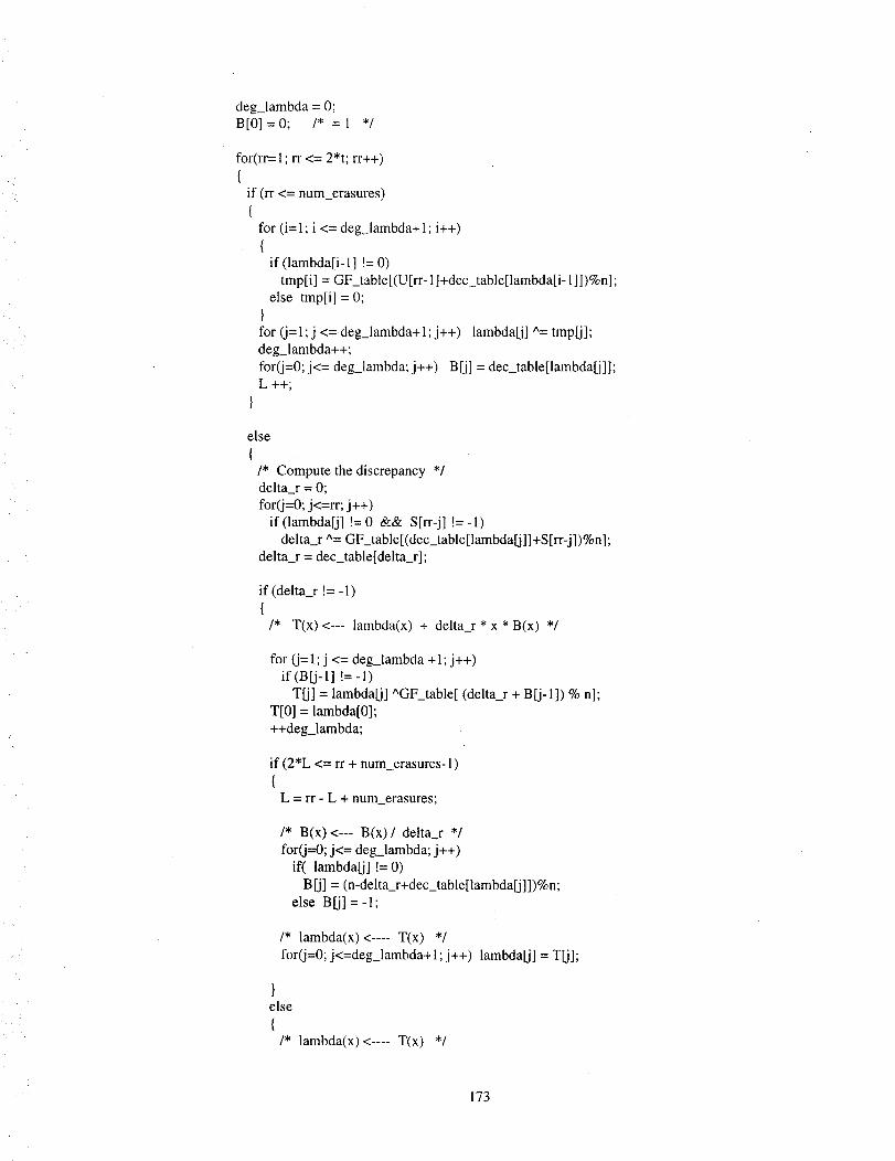
/
deg_lambda = O;B[O] =0; /* = 1 */
for(rr=l; rr <= 2*t; rr++)
{if (rr <= num erasures)
{for (i= 1; i <= deg_lambda+ 1; i++){
if (lambda[i- 1] != 0)
tmp[i] = GF_table[(U[rr- l]+dec table[lambda[i- l]])%n];
else tmp[i] = 0;}for (j=l;j <=deg_lambda+l;j++) lambda[j] ^= tmp[j];deg_lambda++;
for(j=0; j<= deg_lambda; j++) B[j] = dec_table[lambda[j]];L ++;
}
else
{/* Compute the discrepancy */delta_r = O;
for(j=O; j<=rr; j++)
if(lambda[j] !=0 && S[rr-j] !=-l)
delta_r ^= GF_table[(dec_table[lambda[j]]+S[rr-j])%n];delta_r = dec_table[delta_r];
if (delta_r != -1)
/* T(x) <--- lambda(x) + delta_r * x * B(x) */
for (j=l; j <= deg_lambda +1; j++)if (B[i-1] !=-1)
T[j] = lambda[j] aGF_table[ (delta_r + B[j-1]) % n];
T[0] = lambda[0];
++deg_lambda;
if (2*L <= rr + num_erasures-1)
{L = rr - L + num_erasures;
/* B(x)<--- B(x)/ delta_r */
for(j=0; j<= deg_lambda; j++)
if( lambda[j] != 0)
B[j] = (n-delta_r+dec_table[lambda[j]])%n;
else B[j] =-1;
/* lambda(x)< .... T(x) */
for(j=0; j<=deg_lambda+l; j++) lambda[j] = T[j];
}else
{/* lambda(x)< .... T(x) */
173
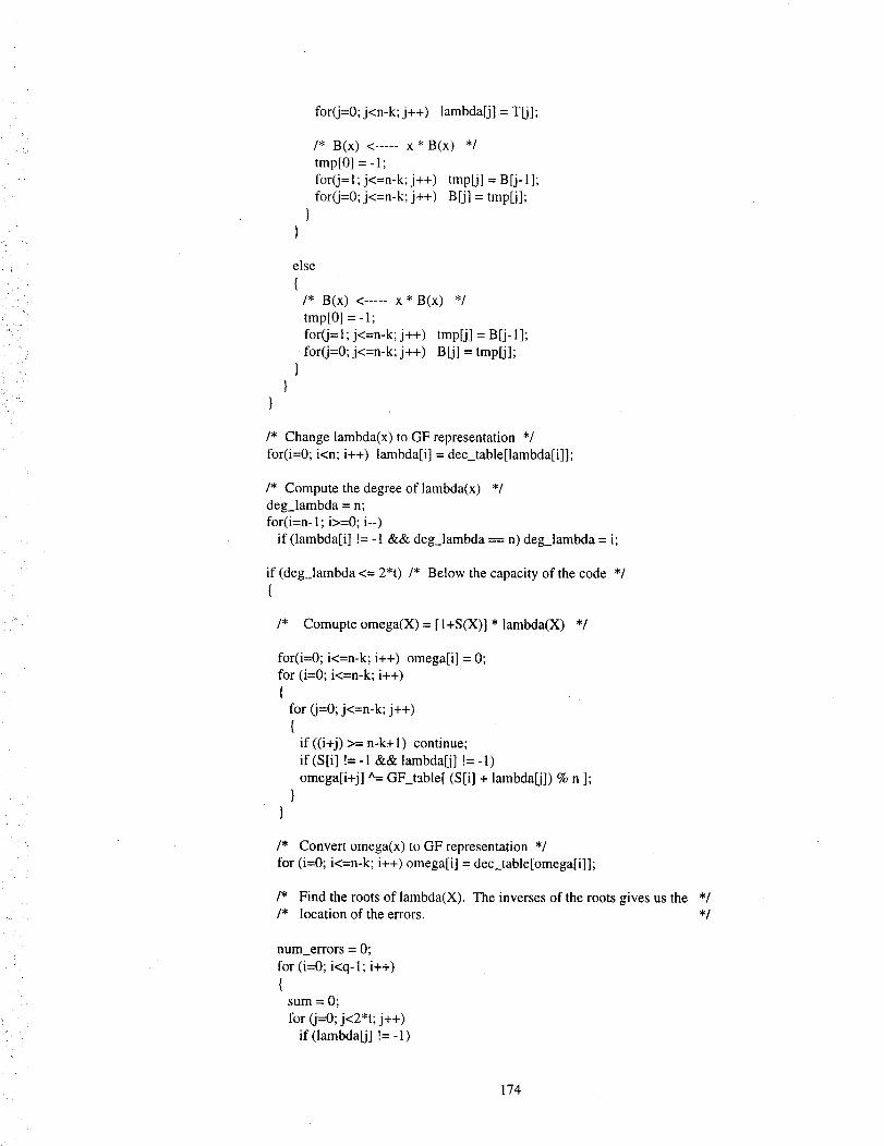
for(j=0;j<n-k;j++) lambda[j]=T[j];
/* B(x) < ..... x* B(x) */
tmp[0] = - 1;
for(j=l; j<=n-k;j++) tmp[j] = B[j-1];for(j=0; j<=n-k; j++) B[j] = tmp[j];
else
/* B(x) <..... x* B(x) */
tmp[0] = - 1;for(j=l; j<=n-k; j++) tmp[j] = B[j- 1];
for(j=0;j<=n-k;j++) B[j] = tmp[j];
/* Change lambda(x) to GF representation */
for(i=0; i<n; i++) lambda[i] = dec_table[lambda[i]];
/* Compute the degree of lambda(x) */deg_lambda = n;for(i=n- 1; i>=0; i--)
if (lambda[i] != -1 && deg_lambda == n) deg_lambda = i;
if (deg_lambda <= 2*t) /* Below the capacity of the code */
/* Comupte omega(X) = [!+S(X)] * lambda(X) */
for(i=0; i<=n-k; i++) omega[i] = 0;for (i=0; i<=n-k; i++)
{for (j=O; j<=n-k; j++){
if ((i+j) >= n-k+l) continue;
if (S[i] != -1 && lambda[j] != -1)
omega[i+j] ^= GF_table[ (S[i] + lambda[j]) % n ];}
}
/* Convert omega(x) to GF representation */for (i=0; i<=n-k; i++) omega[i] = dectable[omega[i]];
/* Find the roots of lambda(X). The inverses of the roots gives us the *//* location of the errors. */
num_errors = 0;
for (i=0; i<q-1; i++){
sum = 0;
for (j=0; j<2*t; j++)if (lambda[j] != - 1)
174
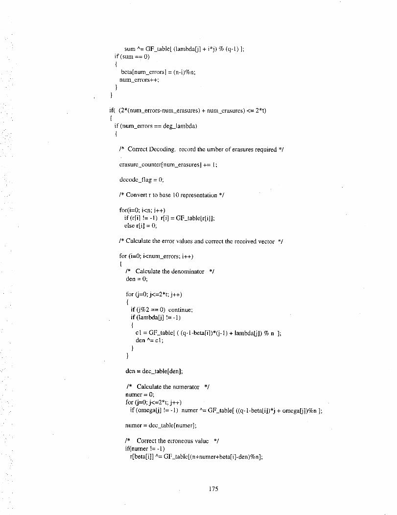
sum =GF_table[(lambda[j]+ i'j) %(q-l)];if (sum==O){
beta[num_errors] = (n-i)%n;
num_errors++;}
if((2*(num_errors-num_erasures) + num_erasures) <= 2*t)
if (num_errors == deg_lambda){
/* Correct Decoding. record the umber of erasures required */
erasure_counter[num_erasures] += l;
decode_flag = 0;
/* Convert r to base 10 representation */
for(i=0; i<n; i++)
if (r[i] != -1) r[i] = GF_table[r[i]];
else r[i] = O;
/* Calculate the error values and correct the received vector */
for (i=O; i<num_errors; i++){
/* Calculate the denominator */
den = O;
for (j=O; j<=2*t; j++)(
if (j%2 == 0) continue;
if (lambda[j] != -1){
cl = GF_table[ ((q-l-beta[i])*(j-1) + lambda[j]) % n ];den ^= c 1;
}}
den = dec_table[den];
/* Calculate the numerator */
numer = 0;
for (j=O; j<=2*t; j++)
if (omega[j] !=- 1) numer ^= GF_table[ ((q- l-beta[i])*j + omega[j])%n ];
numer = dec_table[numer];
/* Correct the erroneous value */
if(numer != - 1)
r[beta[i]] ^= GF_table[(n+numer+beta[i]-den)%n];
175
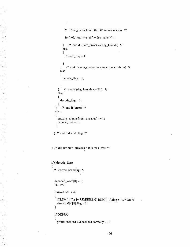
/* Change r back into the GF representation */
for(i=0; i<n; i++) r[i] = dec_table[r[i]];
} /* end if (num_errors == deg_lambda) */else
{decode_flag = 1;
} /* end if (num_erasures + num errors <= dmin) */else
{decode_flag = 1;
} /* end if (deg_lambda <= 2*t) */else
{decode_flag = 1;
}} /* end if(error) */else
{erasure_counter[num_erasures] += 1;
decode_flag = 0;}
} /* end if decode flag */
} /* end for num_erasures = 0 to maxeras */
if (!decode_flag)
{/* Correct decoding. */
decoded_word[ll] = 1;idl +=1;
for(i=0; i<n; i++)
{if(RSM[i][ll].r != RSM[i][II].r2) RSM[i][ll].flag = 1;/* GE */
else RSM[i][ll].flag = 2;}
if(DEBUG)
{printf("\nWord %d decoded correctly", 11);
176
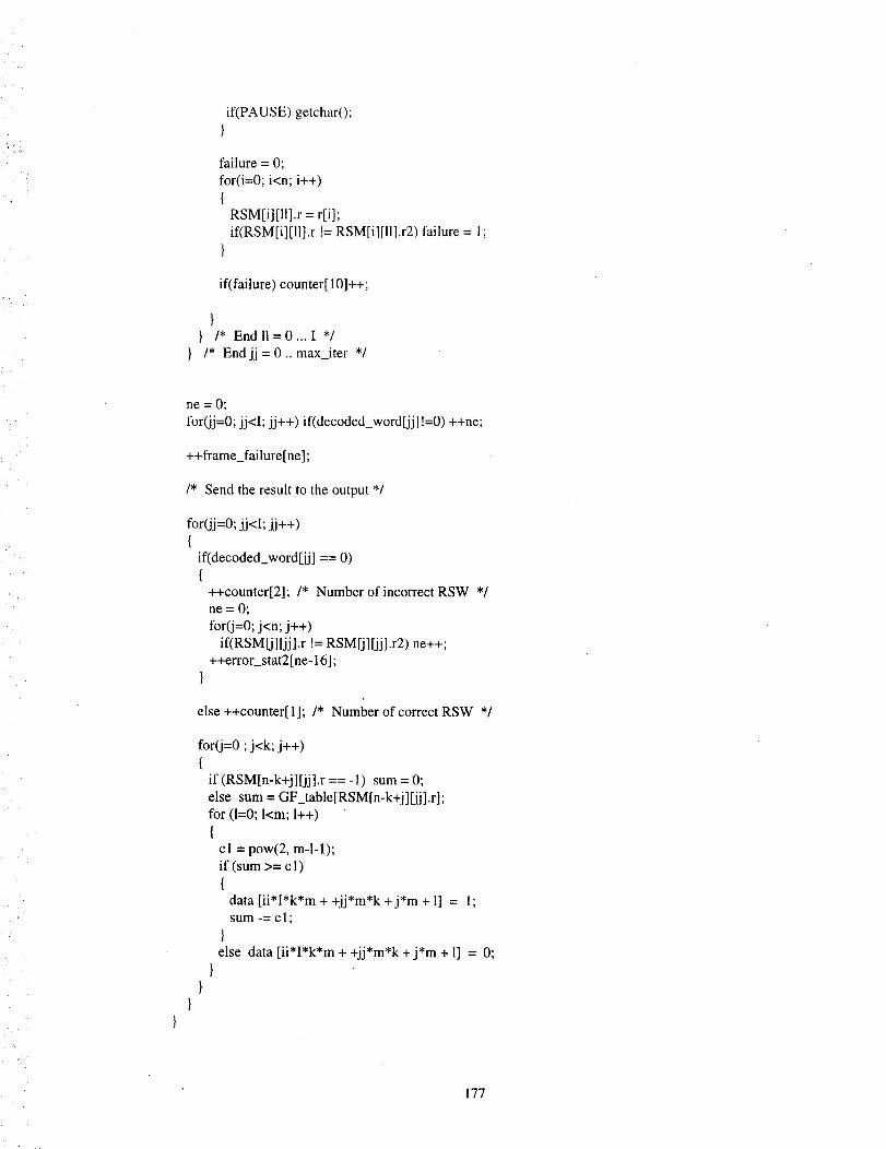
i-
if(PAUSE)getcharO;}
failure = 0;
for(i=0; i<n; i++)
{RSM[i][II].r = r[i];
if(RSM[i][ll].r != RSM[i][I1].r2) failure = 1;
if(failure) counter[ 10]++;
}} /* Endll=0...I */
/* End jj = 0 .. max_iter */
ne = 0;
for(jj=0; jj<I; jj++) if(decoded_word[j j] !=0) ++ne;
++frame_failure[ne];
/* Send the result to the output */
for(jj=0; jj<I; j j++){
if(decoded_word[j j] == 0){
++counter[2]; /* Number of incorrect RSW */
ne = 0;
for(j=0; j<n; j++)
if(RSM[j][jj].r != RSM[j][jj].r2) ne++;
++error_stat2[ne- 16];}
else ++counter[l]; /* Number of correct RSW */
for(j=0 ;j<k; j++){
if (RSM[n-k+j][jj].r == -l) sum = 0;
else sum = GF_table[RSM[n-k+j]W].r];
for (1=0; l<m; 1++)[
cl = pow(2, m-l-l);if (sum >= c 1)
{data [ii*I*k*m + +jj*m*k +j*m + 1] = 1;
sum -= c 1 ;
}else data [ii*I*k*m + +jj*m*k +j*m + 1] = 0;
}}
177
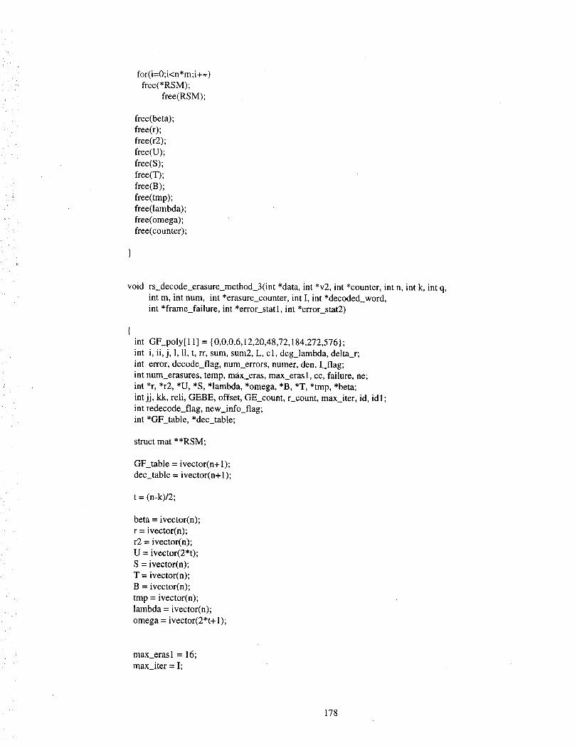
•__i_
for(i=0;i<n*m;i++)free(*RSM);
free(RSM);
free(beta);free(r);free(r2);free(U);free(S);free(T);free(B);free(tmp);free(lambda);free(omega);free(counter);
voidrs_decode_erasure_method_3(int*data,int*v2,int*counter,intn,intk,intq,intm,intnum,int*erasure_counter,intI, int*decoded_word,int*frame_failure,int*error_statl,int *error_stat2)
int GF_poly[11] = {0,0,0,6,12,20,48,72,184,272,576};int i, ii, j, 1,11,t, rr,sum,sum2,L, cl, deg_lambda,delta_r;int error,decode_flag,num_errors,numer,den,I flag;intnum_erasures,temp,max_eras,maxeras1,cc,failure,ne;int*r,*r2,*U,*S,*lambda,*omega,*B,*T,*tmp,*beta;intjj, kk,reli,GEBE,offset,GE_count,r_count,maxiter,id,id1;intredecode_flag,new_info_flag;int*GF_table,*dec_table;
structmat**RSM;
GF_table= ivector(n+1);dec_table=ivector(n+1);
t = (n-k)/2;
beta= ivector(n);r = ivector(n);r2=ivector(n);U=ivector(2*t);S=ivector(n);T=ivector(n);B=ivector(n);tmp=ivector(n);lambda=ivector(n);omega=ivector(2*t+l);
max_erasl= 16;max_iter=I;
178
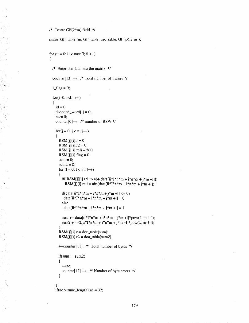
" "S
/* Create GF(2^m) field */
make GF table (m, GF_table, dec_table, GF_poty[m]);
for (ii = 0; ii < num/I; ii ++)
{
/* Enter the data into the matrix */
counter[13] ++; /* Total number of frames */
I_flag = 0;
for(i=0; i<I; i++)
{id = 0;
decoded_word[i] = 0;
ne = 0;
counter[0]++; /* number of RSW */
for(j = 0; j < n; j++)
{RSM[j][i].r = 0;
RSM[j][i].r2 = 0;
RSM[j][i].reli = 500;
RSM[i][i].flag = 0;sum = 0;
sum2 = 0;
for (1 = 0; 1< m; 1++)
{if( RSM[j][i].reli > abs(data[ii*I*n*m + i*n*m + j*m +1]))
RSM[j][i].reli = abs(data[ii*I*n*m + i*n*m + j*m +1]);
if(data[ii*I*n*m + i*n*m + j*m +1] <= 0)
data[ii*I*n*m + i*n*m +j*m +1] = 0;else
data[ii*I*n*m + i*n*m +j*m +1] = 1;
sum += data[ii*I*n*m + i*n*m +j*m +l]*pow(2, m-l-l);
sum2 += v2[ii*I*n*m + i*n*m + j*m +l]*pow(2, m-1-1);}RSM[j][i].r = dec_table[sum];RSM[j] [i].r2 = dec_table[sum2];
++counter[11]; /* Total number of bytes */
if(sum != sum2)
{++ne;
counter[12] ++; /* Number of byte errors */}
if(ne >trunc_length) ne = 32;
179
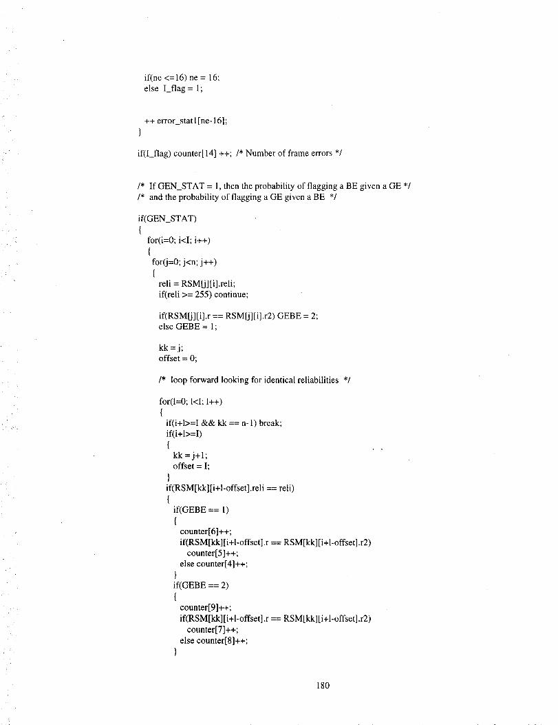
if(ne<=16)ne= 16;elseI_flag= 1;
++error_stat1[ne-16];}
if(I_flag) counter[14] ++; /* Number of frame errors */
/* If GEN_STAT = 1, then the probability of flagging a BE given a GE */
/* and the probability of flagging a GE given a BE */
if(GEN_STAT)
{for(i=0; i<I; i++)
{for(j=0; j<n; j++)
{reli = RSM_][i].reli;if(reli >= 255) continue;
if(RSM[i][i].r == RSM[j][i].r2) GEBE = 2;else GEBE = 1;
kk =j;offset = 0;
/* loop forward looking for identical reliabilities */
for(l=0; 1<I; 1++)
{if(i+l>=I && kk == n-l) break;if(i+l>=I)
{kk =j+l;offset = I;
}if(RSM[kk][i+l-offset].reli == reli)
{if(GEBE == 1)
{counter[6]++;
if(RSM[kk][i+l-offset].r == RSM[kk][i+l-offset].r2)counter[5]++;
else counter[4]++;
}if(GEBE == 2)
{counter[9]++;
if(RSM[kk][i+l-offset].r == RSM[kk][i+l-offset].r2)
counter[7]++;
else counter[8]++;
}
180
}else break;
}
/* loop backwards looking for identical identities */
kk =j;offset = 0;
for(l=0; l<I; 1++)
{if(i-l < 0 && kk == 0) break;
if(i-I < 0)
(kk =j-t;offset = I;
}if(RSM[kkl[i-l+offset].reli == reli){
if(GEBE == 1)
counter[6]++;
if(RSM[kkl[i-l+offset].r == RSM[kk][i-l+offsetl.r2)counter[5]++;
else counter[4]++;
}if(GEBE == 2)
{counter[9]++;
if(RSM[kkl [i-l+offsetl.r == RSM[kk] [i-l+offset].r2)counter[7]++;
else counter[8]++;
}else break;
}/* end loop j = 0 to n */
} /* end loopi=0toI*/} /* end if(GEN_STAT) */
if(DEBUG_DUMP)
(printfC\nDecoded Word\n\n");
for(i=O; i<I; i++) printfC%d\t",decoded_word[i]);
printfC\n");
for(i=0; i<n; i++)
{printfC\n%d ",i);
for(j=0; j<I; j++){
if(RSM[i][i].r != RSM[i][j].r2)
printf("(%d, GE)\t",RSM[i][j].reli);
181
elseprintf("(%d,BE)\t",RSM[i][j].reli);
}}
if(PAUSE) getchar0;
if(DEBUG1)
{
printfC\nReceived word\n");
for(i=0; i<I; i++)
{printfC\n");for(j=0; j<n; j++)
{printfC %d",RSM[j][i].r);
}}
if(PAUSE) getchar0;
printf("\nCon'ect word\n");
for(i=0; i<I; i++)
{printfC\n");
for(j=0; j<n; j++){
printfC %d",RSM[i][i].r2);}
}
if(PAUSE) getchar0;
printf("knReliability\n");
for(i=0; i<I; i++){
printf("_");
for(j=0; j<n; j++)
{printf(" %d",RSM[j][i].reli);
}}
if(PAUSE) getchar0;
printfC\nError flag\n");
182
_.ill(
iI ::i
• .j
for(i=O; i<I; i++)
printfC\n");
for(j=0; j<n; j++)
{printf(" %d",RSM[j][i].flag);
}}
if(PAUSE) getchar0;
} /* end if (DEBUG 1) */
idl = 0;
id = 2;
/* Attempt the iteritive decoding */
for(j j=0; jj<max_iter; jj++){
/* Obtain the reliability info from the enibhoring codewords from */
/* the interleaver and/or SOVA */
if(jj==0) max_eras = 16;
else max_eras = max_eras 1;
if(id 1==id) break;
id=idl;
if(DEBUG)
{printfC\ndecoded word = ");
for(i=0; i<I; i++) printf("%d ", decoded_word[i]);
}
if(id ==I) break;
if(j j==0) redecode_flag = 1;
else redecode_flag = 0;
for(i=I-1; i>=l; i--)
if(decoded_word[i] !=0 && decoded_word[i-1] == O)
redecode_flag = I;
if(!redecode_flag) break;
/* Start prioritising the reliability info, and then begin decoding */
for(ll = 0; 11<I;11++) /* Find good erasures (GE) first */{
GE_count = 0;
if(DEBUG)
{
183
• (i
printf("\ndecoded word = ");for(i=O; i<I; i++) printf("%d ", decoded_word[i]);
if(decoded_word[ll] != 0) continue;
for(i=0; i<n; i++)
{if(RSM[i][ll].flag == 1)
{U[GE_count] = i;
GE_count ++;
}}
if(GE_count < max_eras){
r_count = 0;
for(i=0; i<n; i++)
{if(GE_count + rcount < max_eras)
{if(RSM[i][il].flag == 0){
U[GE_count + r_count] = i;r_count++;
}}
if(GE_count + r_count == max_eras)
{for(j=GE_count; j<max_eras; j++)
{for(l=GE_count; l<max_eras- 1; 1++)
{if(RSM[U[1]][ll].reli > RSM[U[I+I]][II].reli)
{
}}
}
temp = U[I];u[1] = U[l+l];U[I+I] = temp;
r_count ++;
if(GE_count + r_count > max_eras)
{if(RSM[U[max_eras-l]][ll].reli > RSM[i][ll].reli
&& RSM[i][ll].flag == 0)
{
U[max_eras-1] = i;
' 184
for(j=max_eras-1;j>=GE_count+1;j--){
if(RSM[U[j]] [ll].reli < RSM[U[j- 1]][ll].reli){
temp = U[j];uD] = u[j-l];U[j- 1] = temp;
}else break;
} /* End if(GE_count + r_count > max_eras) */
/* End loop i--0..n */} /* End loop if(GE_count < max_eras) */
/* Now we have reliabilities try to decode */
if(DEBUG)
{printfCNumber of trials = %d\n\nMinimum reliabilities and positions\n", counter[ 15]);for(i=0; i<max_eras; i++) printf("(%d, %d)",U[i], RSM[U[i]][ll].reli);
printf("\n");
printf("\nnumber of GE = %d", GE_count);cc = 0;
for(i=0; i<n; i++)
if(RSM[i][ll].r != RSM[i][ll].r2)
cc += 1 ;
printf("\n%d error at %d Reliability = %d", cc, i, RSM[i][ll].reli);for(j=0; j<max_eras; j++)
if(i == U[j]) printfC min %d", j);
if (RSM[i][ll].flag == 1) printf(" GE");}
}if(PAUSE) getchar0;
} /* end if (DEBUG) */
for(i=0; i<n; i++) r[i] = RSM[i][I1].r;
decode_flag = 1;
if(GE_count >= max_erasl) max_eras = GE_count;else max_eras = max_eras 1;
for(num_erasures=GE_count; num_erasures <= max_eras; num_erasures +=2){
185
if(decode_flag){
counter[15] ++; /* Number of decoding trials */
for(i=0; i<num_erasures; i++) r[U[i]] = -1; /* =0 */
error = 0;
/* Compute the syndrome */
for(i=l; i<= n-k; i++)
{s[i] = o;
for(j=0; j<n; j++)
if(r[i] !=-1)
S[i] ^= GF_table[ (r[j] + i'j) % n];if (S[i] != 0) error = 1;/* If nonzero syndrome, there is an error*/
}s[o] = o;
/* Convert to GF representation */
for(i=l; i<=n-k; i++) S[i] = dec table[S[i]];
if (error) /* If the syndrome is equal to zero, no decoding nessasary */{
for(i=0; i < n; i++)
{lambda[i] = 0;
B[i] = -1;
T[i] = 0;}
lambda[0] = GF_table[0];L=0;
deg_lambda = 0;B[0] = 0; /* = 1 '*/
/* =1 */
for(rr= 1; rr <= 2*t; rr++)
(if (rr <= num_erasures)
{for (i=l; i <= deg tambda+l ; i++){
if (lambda[i-l] != 0)
tmp[i] = GF_table[(U[rr- 1]+dec_table[lambda[i- 1]])%n];else tmp[i] = 0;
}
for (j=l; j <= deg_lambda+l; j++) lambda[j] ^= tmp[j];deg_lambda++;
for(j=0; j<= deg_lambda; j++) B_] = dec_table[lambda[j]];L ++;
}
else
{
186

/* Compute the discrepancy */delta r = 0;
for(j=0; j<=rr; j++)
if(lambda[j] != 0 && S[rr-j] != -1)
delta_r ^= GF_table[(dec_table[lambda[j]]+S[rr-j])%n];delta_r = dec_table[delta_r];
if (delta_r != - 1)
{/* T(x) <--- lambda(x) + delta_r * x * B(x) */
,i_I •
for (j=l; j <= deg_lambda +1; j++)
if (B[j-1] !=-I)
T[j] = lambda[j] ^GF_table[ (delta_r + B[j- 1]) % n];T[0] = lambda[0];
++deg_lambda;
if (2*L <= rr + num_erasures-1)
{L = rr - L + num_erasures;
/* B(x)<--- B(x)/ delta_r */
for(j=0; j<= deg lambda; j++)
if( lambda[j] != 0)
B[j] = (n-delta_r+dec_table[lambda[j]])%n;else B[j] =-1;
/* lambda(x)< .... T(x) */
for(j=0; j<=deg_lambda+l; j++) lambda[j] = T[j];
}else
{/* lambda(x)< .... T(x) */
for(j=0; j<n-k;j++) lambda[j] = T[j];
/* B(x) < ..... x* B(x) */
trap[0] = - 1;
for(j=l;j<=n-k;j++) tmp_] = B[j-1];
for(j=O;j<=n-k;j++) B[i] = tmp[j];
else
{/* B(x) < ..... x* B(x) */
tmp[0] = - 1 ;
for(j=l; j<=n-k; j++) tmp[j] = B[j-I];
for(j=0;j<=n-k:j++) B[j] =tmp[j];}
/* Change lambda(x) to GF representation */
for(i=O; i<n; i++) lambda[i] = dec table[lambda[i]];
187
/* Compute the degree of lambda(x) */deg_lambda = n;
for(i=n- 1 ; i>=0; i--)
if (lambda[i] != -1 && deg_lambda == n) deg_lambda = i;
if (deg_lambda <= 2*t) /* Below the capacity of the code */
{
/* Comupte omega(X) = [I+S(X)] * lambda(X) */
for(i=0; i<=n-k; i++) omega[i] = 0;
for (i=0; i<=n-k; i++)
{for (j=0; j<=n-k; j++){
if ((i+j) >= n-k+l) continue;
if (S[i] !=-1 && lambda[j] !=-1)
omega[i+j] ^= GF_table[ (S[i] + lambda[j]) % n ];}
}
/* Convert omega(x) to GF representation */for (i=0; i<=n-k; i++) omega[i] = dec_table[omega[i]];
/* Find the roots of tambda(X). The inverses of the roots gives us the *//* location of the errors. */
num_errors = 0;
for (i=0; i<q-1; i++){
sum = 0;
for (j=0; j<2*t; j++)if (lambda[j] != -1)
sum ^= GF_table[ (lambda[i] + i'j) % (q-l) ];if (sum == 0)
{beta[num_errors] = (n-i)%n;
num_errors++;
}
if((2*(num_errors-num_erasures) + hum_erasures) <= 2*t)
{if (num_errors == deg_lambda)
{
/* Correct Decoding. record the umber of erasures required */
erasure_counter[num_erasures] += 1;
decode_flag = 0;
/* Convert r to base 10 representation */
188
for(i=O;i<n;i++)
if(r[i] !-- -1) r[i] = GF_table[r[i]];
else r[i] = O;
/* Calculate the error values and correct the received vector */
for (i=O; i<num_errors; i++)
{/* Calculate the denominator */
den = O;
for (j=0; j<=2*t; j++){
if (j%2 == 0) continue;
if (lambda[j] != -1){
cl = GF_table[ ((q-l-beta[i])*(j-1) + lambda[j]) % n ];den ^= c 1;
}}
den = dec_table[den];
/* Calculate the numerator */
numer = O;
for (j=O; j<=2*t; j++)
if (omega[j] != - 1) numer ^= GF_table[ ((q- 1-beta[i])*j + omega[j])%n ];
numer = dec_table[numer];
/* Correct the erroneous value */
if(numer != - I)
r[beta[i]] ^= GF_table[(n+numer+beta[i]-den)%n];
/* Change r back into the GF representation */
for(i=O; i<n; i++) r[i] = dec_table[r[i]];
} /* end if (num_errors == deg_lambda) */else
{decode_flag = 1;
}} /* end if (num_erasures +num errors <= dmin) */else
{decode_flag = 1;
}}else
[
/* end if (deg_lambda <= 2*t) */
189
decode_flag= 1;}} /* end if (error) *!else
{erasure_counter[num erasures] += I;
decode_flag = O;
}
} /* end if decode flag *!
} /* end for num_erasures = 0 to max_eras */
if (!decode_flag){
/* Correct decoding. */
decoded_word[ll] = 1;
idl +=l;
for(i=0; i<n; i++){
if(RSM[i][ll].r != RSM[i][II].r2) RSM[i][ll].flag = 1;/* GE */else RSM[i][ll].flag = 2;
}
if(DEBUG){
printf("\nWord %d decoded correctly", 11);
if(PAUSE) getchar0;}
failure = 0;
for(i=0; i<n; i++)
{RSM[i][II].r = r[i];if(RSM[i][ll].r != RSM[i][II].r2) failure = 1;
}
if(failure) counter[ 101++;
/* Begin updating the flags */
?
.i _"
for(j=0; j<n; j++)[
reli = RSM[j][ll].reli;
if(reli >= 255) continue;
GEBE = RSM[j][ll].flag;
190
kk=j;offset= 0;
/* loop forward looking for identical reliabilities */
for(l=0; l<I; 1++)
{if(ll+l>=I && kk == n-1) break;
if(ll+l>=I)
{kk =j+l;offset = I;
}if(RSM[kk] [ll+l-offset].reli == reti)
{if(decoded_word[tl+l-offset] =-- 0)
RSM[kk][ll+l-offset].flag = GEBE;
}else break;
}
/* loop backwards looking for identical identities */
kk =j;offset = 0;
for(l=0; 1<I; 1++)
{if(ll-I < 0 && kk == 0) break;if(ll-I < 0)
{kk =j-l;offset = I;
}if(RSM[kkl[ll-l+offsetl.reli == reli){
if(decoded_word[ll-l+offset] == 0)
RSM[kk] [ll-l+offset].flag = GEBE;
}else break;
}} /* end loopj=0ton*/
decoded_word[i] = 2; /* flag this word as already giving GEBE info */
/* Done revising reliability info */
}} /* Endll=0...I */
/* End jj = 0 .. max_iter */
191
ne=0;for(jj=0;jj<I; jj++)if(decoded_word[jj] !=0)++ne;
++frame_failure[ne];
/* Send the result to the output */
for(j j=0; jj<I; jj++)
{if(decoded_word[j j] == 0)
{++counter[2]; /* Number of incorrect RSW */ne = 0;
for(j=0; j<n; j++)if(RSM[j][jj].r != RSM[j][jj].r2) ne++;
++error_stat2 [ne- 16];}
else ++counter[ I]; /* Number of correct RSW */
for(j=0 ; j<k; j++)[
if (RSM[n-k+j]_jl.r == -1) sum = 0;
else sum = GF table[RSM[n-k+jl[jj].rl;for (1=0; l<m; 1++)
{cl = pow(2, m-l-l);if (sum >= c 1)
{data [ii*I*k*m + +jj*m*k +j*m + 11 = I;
sum -= c 1;
else data [ii*I*k*m + +jj*m*k +j*m + 1] = 0;)
for(i=0;i<n*m;i++)
free(*RSM);
free(RSM);
free(beta);
free(r);
free(r2);
free(U);
free(S);
free(T);free(B);
free(tmp);free(lambda);
free(omega);
192
B.8 Main program for real system using erasure Method I
# include <stdio.h>
# include <math.h>
# include <stdlib.h># include <stddef.h>
# include "mmt31 .h"
# define L_DEBUG 0# define PAUSE 0
# define Nss 16 /* Number of samples per symbol */# define Rb 1 /* The bit rate */
# define Tb (1.0/Rb)
# define Eb 1.0 /* The Energy per bit */
# define Pi 3.14159265359
/* Defining the random number generator constants */
# define IM1 2147483563
# define IM2 2147483399
# define AM (1.0/IM1)
# define IMM1 (IMI-1)# define IA1 40014
# define IA2 40692
# define IQ1 53668# define IQ2 52774# define IR1 12211
# define IR2 3791# define NTAB 32
# define NDIV (I+IMM1/NTAB)# define EPS 1.2e-7
# define RNMX (1.0-EPS)
(
?
void main(int argc, char *argv[]){
int *v, *u, i, ii, errors, M1, M2, Q;long *idum;
long idum_cell;
long num samples, num_bits, N, N_total;
int rs_m, rs_t, rs_n, rs_k, rs_q, rs_num;
int conv_k, conv_n, conv_m, conv_num;double *data, *Tx, *Rx, Pe;
double Psig, EbNo, gain;
int max_repeat, I, rows, I_num, a;
double *xl, *x2;
193
FILE *inpf0,*inpfl, *inpf2,*inpf3,*outf0;
int **soft_metric,*erasure_counter,*rs_counter;int num_erasures;charcFilename[80];
idum---&idum_cell;
EbNo=atof(argv[1]);N=atol(argv[2]);I =atol(argv[31);max_repeat--atol(argv[4]);
sprintf(cFilename,"NewRealM1
inpf0=fopen("m1.dat","r");inpfl =fopen("m2.dat","r");inpf2=fopen("tx.dat","r");inpf3=fopen("rx.dat","r");
_ _erasure%2.2fEbNo_%dI_32delta_8soft.output",EbNo,I);
/* obtain the number of single sided filter *//* coefficents for Tx (M1) and Rx (M2) */
fscanf( inpf0, "%d", &M 1);fscanf(inpfl, "%d", &M2);
Tx = dvector(2*M1);Rx = dvector(2*M2);
xl = dvector(2*Ml+l);
x2 = dvector(2*M2+l);
/* Read in the filter coefficients from data files */
for(i=0; i<2*M1; i++)
fscanf(inpf2, "%lf", &Tx[i]);
for(i=0; i<2"M2; i++)
fscanf(inpf3, "%lf", &Rx[i]);
/* The Reed Solomon coding parameters */
rs_m = 8;
rs_t = 16;
rs_q = pow(2, rs_m);
rs_n = rs_q- 1;rs_k = rs_n - 2*rs_t;
/* Interleaving parameters */
rows = rs_m*rs_n;
194
L
?i
/* The Convolutional coding parameters */
conv_k = 1;
conv_n = 2;
conv_m = 6;
Q = 8i/* Number of soft decision levels */
rsnum = N/(rs k*rs_m);
if( N % (rs_k*rs_m) != O)
{++rs_num;N = rs_num*rs_k*rs_m;
}
I_num = rs_num/I;
if(rs_num%I != 0)
{++ I_num;
rs_num = I_num*I;
N = rs_num*rs_k*rs_m;}
gain = (double)(conv_k*rs_k)/(conv_n*rs n);
a = 10.0;
conv_num = (rs_num*rs_n*rs_m + 50)/conv_k;num_bits = conv_n*(conv_num + 100);
num_samples = num_bits*Nss;errors = O;
erasure_counter = ivector(2*rs_t);rs_counter = ivector(rs_t);
soft_metric = int_matrix_2d(2, Q);
for(i=0; i<6; i++) rs_counter[i] = 0;
N_total = 0;
data = dvector(num_samples+3*M 1);
v = ivector(num_bits);u = ivector(N);
*idum = -10;
195
?
for(ii=0; ii<max_repeat; ii++)
for (i=0; i<num_bits; i++) v[i] = 0;
for (i=0; i<N; i++)
{v[i] = bitgen(idum);u[i] = vii];
}
rs_encode(v, rs_n, rs_k, rs_m, rs_num);
interleave(v, rows, rs_n, rs_m, I, I_num);
conv_encode(v, conv_n, conv_k, conv_m, conv_num);
modulate(data, v, num_bits);
filter(data, M1, Tx, xl, num_samples);
/* Adjust for delay introduced by filter */
for(i=0; i<num_samples; i++)data[i] = data[i+M 1];
Psig = calc_power(data, num_samples);
add_noise(idum, data, num_samples, Psig, EbNo, gain);
filter(data, M2, Rx, x2, num_samples);
/* Adjust for delay introduced by filter */
for(i=0; i<num_samples; i++)data[i] = data[i+M2];
demodsoft(data, v, num_bits, soft_metric, Q, a);
conv_decode(v, conv_n, conv_k, conv_m, conv_num, soft_metric, a);
deinterleave(v, rows, rs_n, rs_m, I, I_num);
rs_decode(v, rs_n, rs_k, rs_q, rs_m, rs_num, erasure_counter, rs_counter);
for (i=0; i<N; i++)
if (v[i] != u[i])
{errors += l;
}
196
h :
N_total += N;
outf0=fopen(cFilename,"at+");for (i=0; i<=rs_t; i+=2)fprintf(outf0,"%de= %d ",i, erasure_counter[i]);
fprintf(outf0,"\nnum = %d\n\nRS counter = ",rs_num);
for(i=0; i<6; i++) fprintf(outf0," %d",rs_counter[i]);
fprintf(outf0,"Xn\nl. S = 0. No Decoding\n2. deg_lambda > 2*t");
fprintf(outf0,"Xn3. 2*e + f > 2*tXn4. num_errors != deg_lambda");
fprintf(outf0,"\n5. Correct decoding\n5. Incorrect Decoding");
fprintf(outfO,"\nknEb/No = %2.2f dB",EbNo);
fprintf(outf0,"\n(%d, %d, %d) Reed Solomon Code",rs_n, rs_k, rs_t);
fprintf(outf0,"\ninterleaving depth I = %d",I);fprimf(outfO,"\n(%d, %d, %d) convolutional code", conv_n, cony_k, conv_m);
fprintf(outf0,"\niteration number = %d\n# errors = %d\n N total = %ld", ii+ 1, errors, N_total);Pe = (float)errors/N_total;
fprintf(outf0,"\nPe = %2. lOf_n\n",Pe);
fclose(outf0);
outf0=fopen(cFilename,"at+");
fpri ntf(outf0,"knerasure counter = ");
for (i=0; i<=rs_t; i+=2) fprintf(outf0,"%de= %d ",i, erasure_counter[i]);
fprintf(outf0,"\nnum = %d\nknRS counter = ",rs_num);
for(i=0; i<6, i++) fprintf(outf0," %d",rs_counter[i]);
fprintf(outf0,"\nXnl. S = 0. No Decoding\n2. deg_lambda > 2*t");
fprintf(outf0,"\n3. 2*e + f > 2*tkn4. num_errors != deg_lambda");
fprintf(outf0,"\n5. Correct decodinghaS. Incorrect Decoding");
fprintf(outf0,"_Eb/No = %2.2f dB",EbNo);
fprintf(outf0,"\nNumber of erasures = %d", num_erasures);
fprintf(outf0,"kn(%d, %d, %d) Reed Solomon Code",rs_n, rs_k, rst);
fprintf(outf0,"kninterleaving depth I = %d",I);
fprintf(outf0,"_(%d, %d, %d) convolutional code", conv_n, conv_k, conv_m);
fprintf(outfO,"\niteration number = %d\n# errors = %dXn N total = %ld", ii+l, errors, Ntotal);Pe = (float)errors/N_total;
fprintf(outf0,"\nPe = %2.10f_nXn",Pe);
fclose(outf0);
fclose(inpfl);
fclose(inpf2);fclose(inpf3);
free(xl);free(x2);
free(data);
197
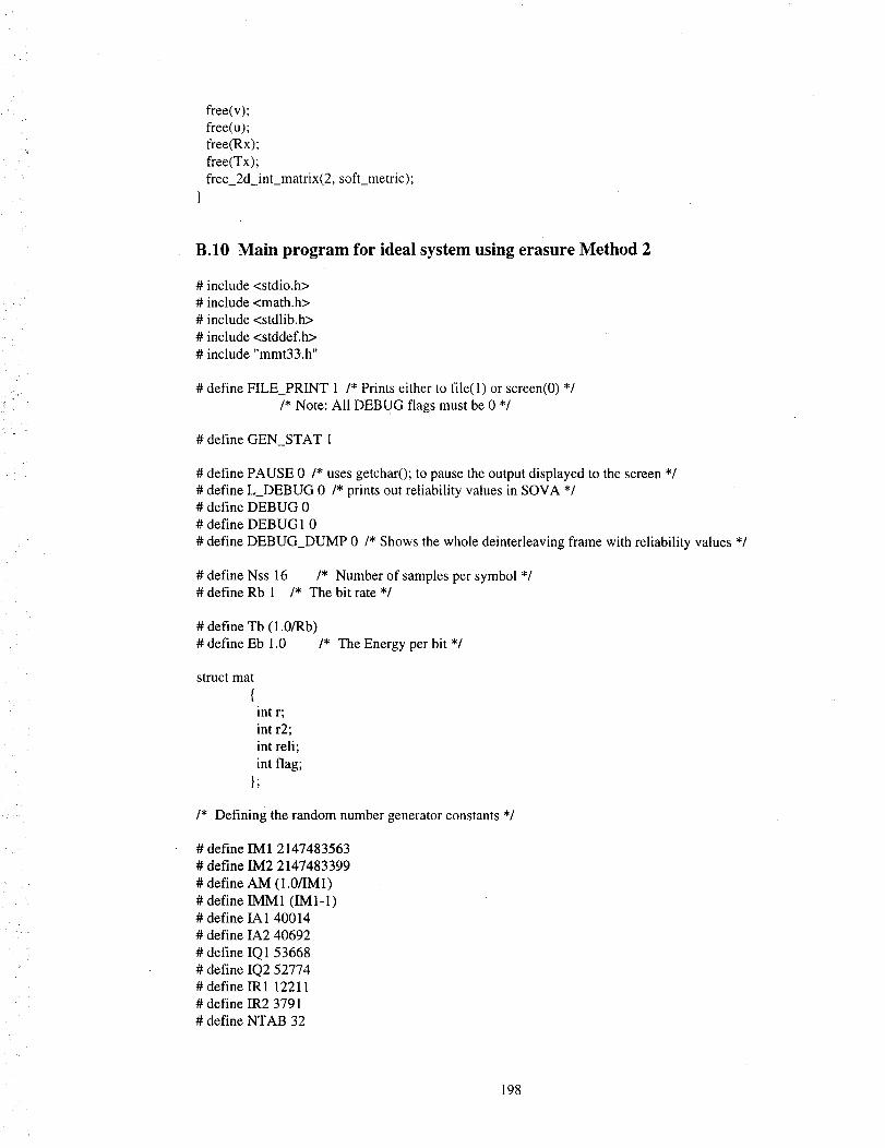
free(v);free(u);free(Rx);free(Tx);free2d int matrix(2,soft_metric);
B.10 Main program for ideal system using erasure Method 2
# include <stdio.h># include <math.h>
# include <stdlib.h># include <stddef.h>
# include "mmt33.h"
# define FILE_PRINT 1 /* Prints either to file(l) or screen(0) */
/* Note: All DEBUG flags must be 0 */
# define GEN_STAT I
# define PAUSE 0 /* uses getchar0; to pause the output displayed to the screen */# define L_DEBUG 0 /* prints out reliability values in SOVA */# define DEBUG 0# define DEBUG1 0
# define DEBUG_DUMP 0 /* Shows the whole deinterleaving frame with reliability values */
# define Nss 16 /* Number of samples per symbol */# define Rb 1 /* The bit rate */
# define Tb (1.0/Rb)
# define Eb 1.0 /* The Energy per bit */
struct mat
{int r;
int r2;
int reli;
int flag;};
/* Defining the random number generator constants */
# define lM1 2147483563
# define lM2 2147483399
# define AM(1.0/IMI)
# define IMM 1 (IM 1-1)# define IA1 40014
# define IA2 40692
# define IQ1 53668# define IQ2 52774# define IR1 12211
# define IR2 3791
# define NTAB 32
198
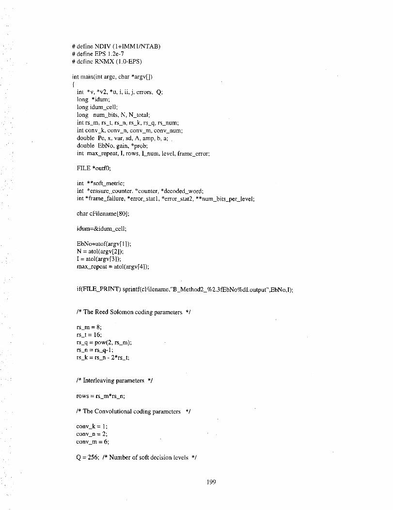
j
# define NDIV (1 +IMM 1/NTAB)# define EPS 1.2e-7
# define RNMX (1.0-EPS)
int main(int argc, char *argv[]){
int *v, *v2, *u, i, ii, j, errors, Q;
long *idum;
long idum cell;
long num_bits, N, N_total;
int rs_m, rs_t, rs_n, rs_k, rs_q, rs_num;int conv_k, conv_n, conv_m, conv_num;
double Pe, x, var, sd, A, amp, b, a;
double EbNo, gain, *prob;int max_repeat, I, rows, I_num, level, frame_error;
FILE *outf0;
int **soft_metric;
int *erasurecounter, *counter, *decoded_word;
int *frame_failure, *error_statl, *error_stat2, **num_bits_per_level;
char cFilename[80];
idum=&idum_cell;
EbNo=atof(argv [ 1]);
N = atol(argv[2]);I = atol(argv[3]);
max_repeat = atol(argv[4]);
if(FILE_PRINT) sprintf(cFilename,"B_Method2_%2.3fEbNo%dI.output",EbNo,I);
/* The Reed Solomon coding parameters */
rs_m = 8;
rs_t = 16;
rs_q = pow(2, rs_m);
rs_n = rs_q- 1;rs_k = rs_n - 2*rs_t;
/* Interleaving parameters */
rows = rs_m*rs_n;
/* The Convolutional coding parameters */
conv_k = 1;
conv_n = 2;
conv_m = 6;
Q = 256; /* Number of soft decision levels */
199
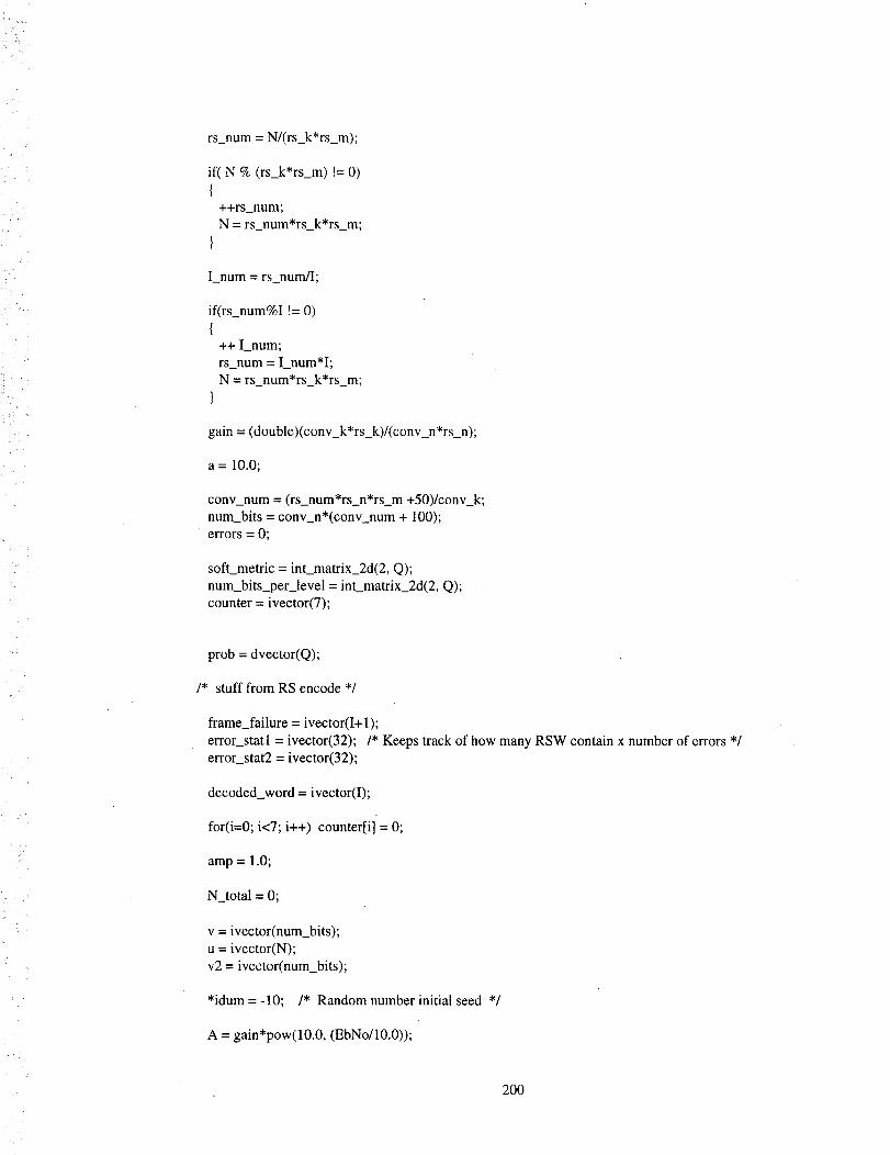
rs_num=N/(rs_k*rs_m);
if(N%(rs_k*rs_m)!=0){
++rs_num;
N = rs num*rs_k*rs_m;
I_num = rs_num/I;
if(rs_num%I != 0)
{++ I_num;
rs_num = I_num*I;
N = rs_num*rs_k*rs_m;
}
gain = (double)(conv_k*rs_k)/(conv_n*rs_n);
a = 10.0;
conv_num = (rs_num*rs_n*rs_m +50)/conv k;
num_bits = conv_n*(conv_num + 100);errors = O;
soft_metric = int_matrix_2d(2, Q);
num_bits_per_level = int_matrix_2d(2, Q);counter = ivector(7);
prob = dvector(Q);
/* stuff from RS encode */
frame_failure = ivector(I+ 1);
error_statl = ivector(32); /* Keeps track of how many RSW contain x number of errors */error_stat2 = ivector(32);
decoded_word = ivector(I);
for(i=0; i<7; i++) counter[i] = 0;
amp = 1.0;
N_total = 0;
v = ivector(num_bits);
u = ivector(N);
v2 = ivector(num_bits);
*idum = -10; /* Random number initial seed */
A = gain*pow(10.0, (EbNo/10.0));
20O
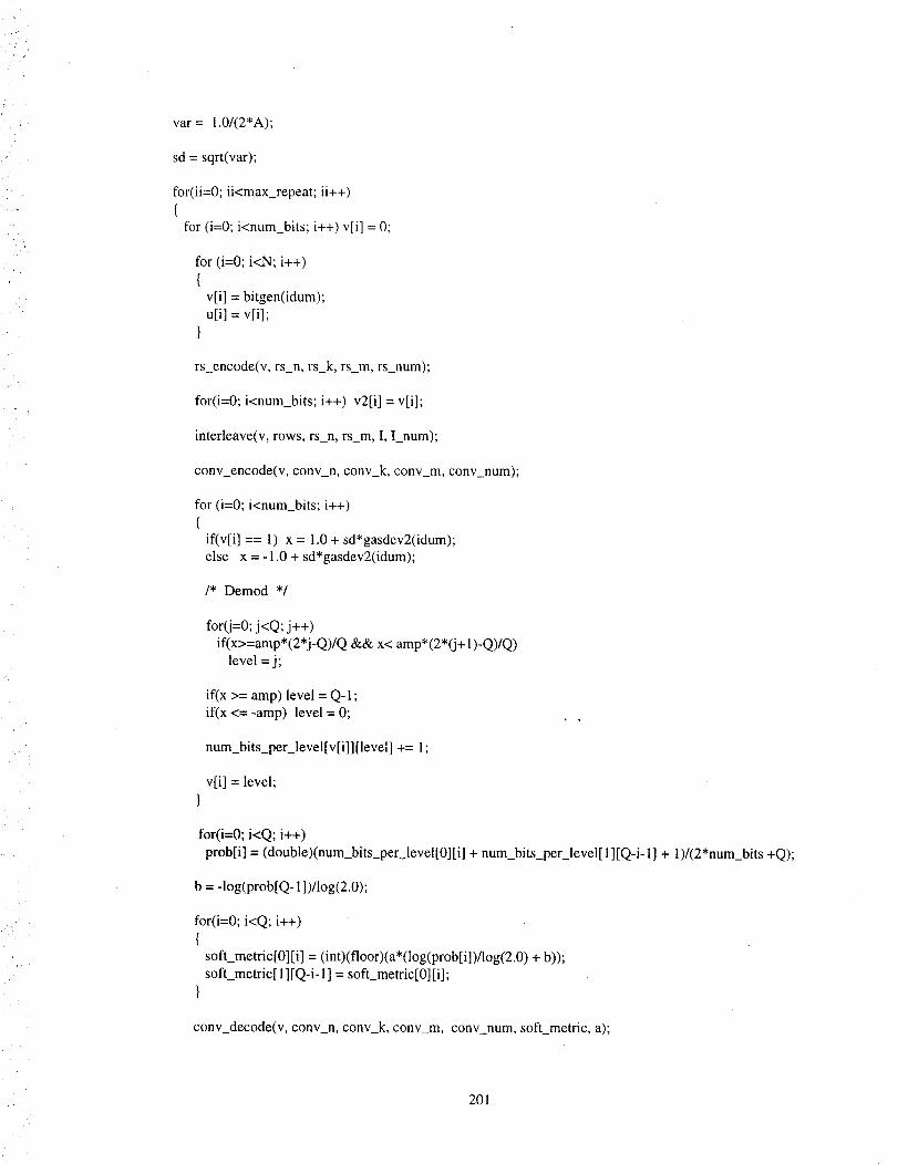
var= 1.0/(2*A);
sd= sqrt(var);
for(ii=0;ii<max_repeat;ii++){
for (i=0; i<num_bits; i++) vii] = 0;
for (i--0; i<N; i++)
{v[i] = bitgen(idum);
u[i] = v[i];}
rs_encode(v, rs_n, rs_k, rs_m, rs_num);
for(i=0; i<num_bits; i++) v2[i] = v[i];
interleave(v, rows, rs_n, rs_m, I, I_num);
conv_encode(v, conv_n, conv_k, conv_m, conv_num);
for (i=0; i<num_bits; i++)
{if(v[i] == 1) x = 1.0 + sd*gasdev2(idum);
else x = - 1.0 + sd*gasdev2(idum);
/* Demod */
for(j=0; j<Q; j++)
if(x>=amp*(2*j-Q)/Q && x< amp*(2*(j+ 1)-Q)/Q)
level = j;
if(x >= amp) level = Q- 1;
if(x <= -amp) level = O;
num_bits_per_level[v[i]][level] += 1;
v[i] = level;}
for(i=O; i<Q; i++)
prob[i] = (double)(num_bits_per_level[O] [i] + num_bits_per_level[ 1][Q-i- 1] + 1)/(2*num_bits +Q);
b = -log(prob[Q- 1])/log(2.0);
for(i=O; i<Q; i++)
{
soft_metric[O][i] = (int)(floor)(a*(log(prob[i])/log(2.0) + b));soft_metric[ 1][Q-i- 1] = soft_metric[O][i];
}
conv_decode(v, conv_n, conv_k, conv_m, conv_num, soft_metric, a);
201
ii • :
deinterleave(v, rows, rs_n, rsfm, I, I_num);
rs_decode_erasure_method_2(v, v2, counter, rs_n, rs_k, rs_q, rs_m, rs_num,erasure_counter, I, decoded_word, frame_failure, error_statl, error_stat2);
for (i=0; i<N; i++)
if (v[i] != u[i])
errors += 1 ;
N_total += N;
if(!FILE_PRINT){
printf("\n\n");printf("Erasure Counter\n");
for (i=0; i<=2*rs_t-4; i+=2) printf("%de= %d ",i, erasure_counter[i]);
printf("\n\nError Counter 1 (number of times x amount of errors occoured)\n");
for(i=0; i<16; i++)
{if(i==7) printf("\n");
printf("%derr = %d ", 16+i, error_statl [i]);
}
printf("\n\nError Counter 2 (# of errors for non-decoded word)\n");
for(i=0; i<16; i++)
{if(i==7) printf("\n");
printf("%derr = %d ", 16+i, error_stat2[i]);}
printf("\n\nFrame decoded with x correct\n");
for(i=0; i<=I; i++) printf("%dcct = %d ",i, frame_failure[i]);
if(GEN_STAT)
{printf("_\nNumber of GE flagged GE = %d Prob = % 1.3f_n", counter[4],
(float)counter[4]/counter[6]);
printf("Number of GE flagged BE = %d Prob = % 1.3f_n",
counter[5],(float)counter[5]/counter[6]);
printf("Total number of GE declaired = %d\n",counter[6]);
printf("\nNumber of BE flagged BE = %d Prob = % 1.3f_n", counter[7],(float)counter[7]/counter[9]);
printf("Number of BE flagged GE = %d Prob = % 1.3f_n", counter[8],(float)counter[8]/counter[9]);
printf("Total number of BE declaired = %d\n",counter[9]);}
printf("\n\nBefore Decoding, no erasures used:\n");
202
2
printf("\nTotal number of bytes = %d", counter[l 1]);
printfC\nNumber of byte errors = %d", counter[12]);
printf("\nProb of byte error = %2.51f",(double)counter [ 12]/counter[ 1 t]);
printf("\n\nTotal number of frames = %d", counter[13]);
printfC\nNumber of frames in error = %d", counter[ 14]);
printfC\nProb of frame error = %2.51f", (double)counter[ 14]/counter[13]);
printfc\n\nNumber of RSW = %d",counter[0]);
printfC\nNumber of RSW correct = %d",error_statl [0]);printf("\nNumber of RSW incorrect = %d", counter[0]-error_stat 1 [0]);
printfC\nProb of RSW incorrect = %2.5 If" ,(double)(counter[0]-error_stat 1 [0] )/counter[0] );
printfC\n\nAfter decoding:\n");
frame_error = O;
for(i=O; i<I; i++) frame_error += frame failure[i];
printf("\nTotal number of frames = %d", counter[ 13]);
printf("\nNumber of frames in error = %d", frame_error);
printf("\nProb of frame error = %2.51f",(double)frame_error/counter[ 13]);
printf("\n\nNumber of RSW = %d",counter[0]);printf("\nNumber of RSW correct = %d",counter[ 1]);
printf("\nNumber of RSW incorrect = %d", counter[2]);
printfC\nProb of RSW incorrect = %2.51f",(double)counter[2]/counter[0]);
printf("\n\nTotal number of decoding trials = %d",counter[ 15]);
printf("\nAverage number of decoding trials = %3.31f", (double)counter[ 15]/counter[0]);
printfC\nNumber of decoding failures = %d\n",counter[10]);
printf("\n\nEb/No = %2.2f dB",EbNo);
printf("\n(%d, %d, %d) Reed Solomon Code",rs_n, rs_k, rs_t);printf("\ninterleaving depth I = %d",I);
printf("ha(%d, %d, %d) convolutional code", conv_n, conv_k, conv_m);
printf("_niteration number = %d\n# errors = %d\n N total = %ld", ii+ 1, errors, N_total);Pe = (float)errors/N_total;
printf("haPe = %2.1015n\n",Pe);
if(FILE_PRINT){
outf0=fopen(cFilename,"at+");
fprintf(outf0,"\n\nErasure Counter\n");
for (i=0; i<=2*rs_t-2; i+=2) fprintf(outf0,"%de= %d ",i, erasure_counter[i]);
fprintf(outf0,"\n\nError Counter 1 (number of times x amount of errors occoured)\n");
203
for(i=0;i<16;i++)fprintf(outf0,"%derr= %d", 16+i,error_statl[i]);
for(i=0;i<16;i++){
if(i==7) fprintf(outf0,"\n");
fprintf(outf0,"%derr = %d ", 16+i, error_statl[i]);}
fprintf(outf0,"\n\nError Counter 2 (# of errors for non-decoded word)in");
for(i=0; i<16; i++)
{if(i==7) fprintf(outf0,"\n");
fprintf(outf0,"%derr = %d ", 16+i, error_stat2[i]);}
fprintf(outf0,"\n\nFrame decoded with x correct\n");
for(i=0; i<=I; i++) fprintf(outf0,"%dcct = %d ",i, frame failure[i]);
if(GEN_STAT)
[fprintf(outf0,"\n\nNumber of GE flagged GE = %d Prob = % 1.315n", counter[4],
(float)counter[4]/counter[6]);
fprintf(outf0,"Number of GE flagged BE = %d Prob = % 1.315n",counter[5],(float)counter[5]/counter[6]);
fprintf(outf0,"Total number of GE declaired = %d\n",counter[6]);
fprintf(outf0,"\nNumber of BE flagged BE = %d Prob = % 1.3f_n", counter[7],(float)counter[7]/counter[9]);
fprintf(outf0,"Number of BE flagged GE = %d Prob = % 1.3f_n", counter[8],(float)counter[8]/counter[9]);
fprintf(outf0,"Total number of GE declaired = %d\n",counter[9]);}
fprintf(outf0,"\n_Before Decoding, no erasures used:\n");
fprintf(outf0,"\nTotal number of bytes = %d", counter[11]);
fprintf(outf0,"_Number of byte errors = %d", counter[ 12]);
fprintf(outf0,"\nProb of byte error = %2.51f',(double)counter[ 12]/counter[ 11]);
fprintf(outf0,"\n\nTotal number of frames = %d", counter[ 13]);
fprintf(outf0,"\nNumber of frames in error = %d", counter[ 14]);
fprintf(outf0,"\nProb of frame error = %2.51f", (double)counter[ 14]/counter[ 13]);
fprintf(outf0,"\n\nNumber of RSW = %d",counter[0]);
fprintf(outf0,"\nNumber of RSW correct = %d",error_statl [0]);
fprintf(outf0,"\nNumber of RSW incorrect = %d", counter[0]-error_stat 1[0]);
fprintf(outf0,"\nProb of RSW incorrect = %2.51f",(double)(counter[0]-error_statl [0])/counter[0]);
fprintf(outf0,"\n\nAfter decoding :in");
frame_error = 0;
204
for(i=0;i<I;i++)frame_error+=frame_failure[i];
fprintf(outf0,"\nTotalnumberofframes=%d",counter[13]);fprintf(outf0,"\nNumberofframesinerror=%d",frame_error);fprintf(outf0,"\nProbofframeerror=%2.51f",(double)frame_error/counter[l3]);
fprintf(outf0,"\n\nNumberofRSW=%d",counter[0]);fprintf(outf0,"\nNumberofRSWcorrect= %d",counter[1]);fprintf(outf0,"\nNumberofRSWincorrect= %d",counter[2]);fprintf(outf0,"\nProbof RSWincorrect= %2.51f",(double)counter[2]/counter[0]);
fprintf(outf0,"\n\nTotalnumberofdecodingtrials= %d",counter[15]);fprintf(outf0,"\nAveragenumberofdecodingtrials= %3.31f",(double)counter[15]/counter[0]);
fprintf(ouff0,"\nNumberofdecodingfailures= %d\n",counter[10]);
fprintf(outf0,"\n\nEb/No= %2.2fdB",EbNo);fprintf(outf0,"\n(%d,%d,%d)ReedSolomonCode",rs_n,rs_k,rs_t);fprintf(outf0,"\ninterleavingdepthI =%d",I);fprintf(outf0,"\n(%d,%d,%d)convolutionalcode",conv_n,conv_k,conv_m);fprintf(outf0,"\niterationnumber=%d\n#errors= %d\nNtotal=%ld",ii+l, errors,N_total);Pe= (float)errors/N_total;fprintf(outf0,"\nPe= %2.10f_n\n",Pe);
fclose(outf0);}
free(v);
free(u);
free(v2);
free 2d int matrix(2, soft_metric);
free 2d int matrix(2, num_bits_per_level);free(decoded_word);
free(frame_failure);
free(error_stat 1);free(error stat2);
205

k
..H:/ /
[1]
[2]
[3]
[4]
[5]
[6]
[71
[8]
References
Berrou, Claude., Adde, Patrick., Ettiboua., and Faudeil, Stephane., "A Low
Complexity Soft-Output Viterbi Decoder Architecture,". Procedings ICC '93, pp.
737 -740. May 1993.
Blahut, R. E., Theory. and Practice of Error Control Codes, Addison Wesley,
Reading Mass., 1984.
Fomey, G. D., "On Decoding BCH Codes," IEEE Transactions on Information
Theory, Volume IT-11, pp. 393-403, October 1965.
Hagenauer, J. and Hoeher, P., "A Viterbi Algorithm with Soft Outputs and Its
Applications," Procedings of the IEEE Globecomm Conference, Dallas, Tex., pp.
47.1.1-47.1.7, November 1989.
Jeruchim, Michael C., Balaban, Philip., and Shanmugan, K. Sam., Simulation of
Communication Systems., Plentum Press, New York_ NY., 1992.
Lin, S., and Costello, D. J., Jr., Error Control Coding: Fundamentals and
Applications, Prentice-Hall, Inc., Englewood Cliffs, NJ., 1983.
Paaske, Eric, "Improved Decoding for a Concatenated Coding System
Recomended by CCSDS," IEEE Transactions on Communications, Volume
COM-38, pp. 1138-1144, August 1990.
Press, W. H., Teukolsky, S. A., Vettering, W. T., Flannery, B. P., Numerical
Recipies in C., Cambridge University Press., 1992.
2o6
[9]
[I0]
[11]
[12]
[13]
[14]
[15]
[16]
Sklar, Bernard, Digital Communications: Fundamentals and Applications,
Prentice Hall, Inc., Englewood Cliffs, NJ., 1988.
Viterbi, Andrew J., Omura, Jim K., Principles of Digital Communication and
Coding, McGraw-Hill, New York, NY., 1979.
Wicker, Stephen B., Error Control Systems for Digital Communication and
Storage, Prentice-Hall, Inc., Englewood Cliffs, NJ., 1995.
Pratt, Timothy., Bostian, Charles., Satellite Communications. John Willey and
Sons., New York, NY., 1976.
Palmer, Larry C., "Computer Modeling and Simulation of Communications
Satellite Channels,". IEEE Journal on Selected Areas of Communications,
Volume SAC-2, No. 1, pp. 89-102, January 1984.
Hagenaurer, J., Offer, E., and Papke, L., "Matching Viterbi Decoders and Reed
Solomon Decoders in a Concatenated System,". Reed Solomon Codes and their
Applications, Ch. 11, edited by Wicker, S., and Bhargava, V., IEEE Press, New
York, NY., 1994.
Wicker, S., and Bhargava, V., "An Introduction to Reed Solomon Codes,". Reed
Solomon Codes and their Applications, Ch. 1, edited by Wicker, S., and
Bhargava, V., IEEE Press, New York, NY., 1994.
McEliece, Robert., Swanson, Liaf., "Reed Solomon Codes and the Exploration of
the Solar System,". Reed Solomon Codes and their Applications, Ch. 3, edited by
Wicker, S., and Bhargava, V., IEEE Press, New York, NY., 1994.
207
"i [17]
[18]
[19]
Massey, J. L., "Shift Register Synthesis and BCH Decoding," IEEE Transactions
on Information Theory, Vol. IT-15, No. 1, pp. 122-127, Jan. 1969.
Feher, Kamilo., Digital Communications Satellite�Earth Station Engineering.,
Prentice Hall, Englewood Cliffs, N. J. 1985.
McEliece, Robert, and Swanson, Liaf., "On the decoder error probability of Reed-
Solomon codes," IEEE Transactions on Information Theory, Vol. IT-32, pp 701-
703, Sept. 1986.
208

Pr
p_ • iI_I_¸II_ r___._


![Contents · Figure 1.2: The (n,k,ν) convolutional encoder In 1976, Viterbi [1] introduced a decoding algorithm for convolutional code. And Omura [2] showed that the Viterbi Algorithm](https://img.pdfslide.us/doc/110x75/5e98b65866b80e2e6461d1ff/contents-figure-12-the-nk-convolutional-encoder-in-1976-viterbi-1-introduced.jpg)


![Unifying Performance Metric of Viterbi Decoders · 2.1 Rate-1/2 convolutional encoder with generator polynomials (G0=5, ... [3, 4, 5, 6, 7, 8]. ... of the Viterbi decoder come up](https://img.pdfslide.us/doc/110x75/5b62c25c7f8b9a54488de550/unifying-performance-metric-of-viterbi-decoders-21-rate-12-convolutional-encoder.jpg)