NASA Approach to

Vicarious Calibration

IOCCG Vicarious Calibration Workshop

November 2013

Bryan Franz

and the

Ocean Biology

Processing Group

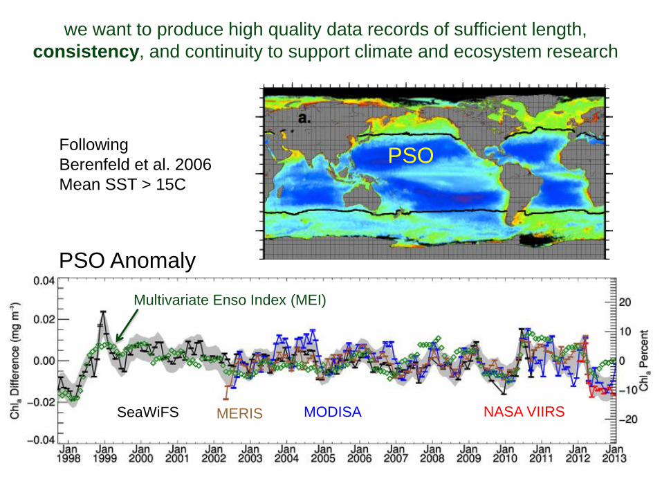
we want to produce high quality data records of sufficient length,

consistency, and continuity to support climate and ecosystem research

PSO Anomaly

SeaWiFS MODISA NASA VIIRS MERIS

Multivariate Enso Index (MEI)

PSO Following

Berenfeld et al. 2006

Mean SST > 15C

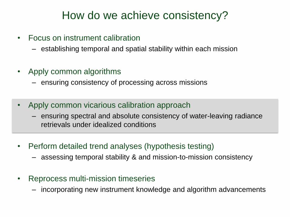
How do we achieve consistency?

• Focus on instrument calibration

– establishing temporal and spatial stability within each mission

• Apply common algorithms

– ensuring consistency of processing across missions

• Apply common vicarious calibration approach

– ensuring spectral and absolute consistency of water-leaving radiance

retrievals under idealized conditions

• Perform detailed trend analyses (hypothesis testing)

– assessing temporal stability & and mission-to-mission consistency

• Reprocess multi-mission timeseries

– incorporating new instrument knowledge and algorithm advancements

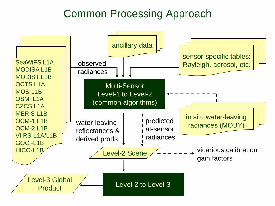
Common Processing Approach

Multi-Sensor

Level-1 to Level-2

(common algorithms)

SeaWiFS L1A

MODISA L1B

MODIST L1B

OCTS L1A

MOS L1B

OSMI L1A

CZCS L1A

MERIS L1B

OCM-1 L1B

OCM-2 L1B

VIIRS-L1A/L1B

GOCI-L1B

HICO-L1B

Level-2 to Level-3

Level-2 Scene

observed

radiances

ancillary data

water-leaving

reflectances &

derived prods

Level-3 Global

Product

vicarious calibration

gain factors

predicted

at-sensor

radiances

in situ water-leaving

radiances (MOBY)

sensor-specific tables:

Rayleigh, aerosol, etc.

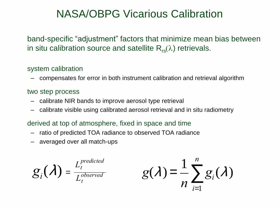
NASA/OBPG Vicarious Calibration

band-specific “adjustment” factors that minimize mean bias between

in situ calibration source and satellite Rrs(l) retrievals.

system calibration

– compensates for error in both instrument calibration and retrieval algorithm

two step process

– calibrate NIR bands to improve aerosol type retrieval

– calibrate visible using calibrated aerosol retrieval and in situ radiometry

derived at top of atmosphere, fixed in space and time

– ratio of predicted TOA radiance to observed TOA radiance

– averaged over all match-ups

 

gi(l) =Ltpredicted

Ltobserved g(l) =

1

ngi(l)

i=1

n

å

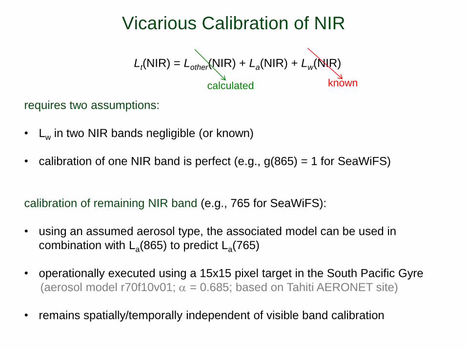
Lt(NIR) = Lother(NIR) + La(NIR) + Lw(NIR)

requires two assumptions:

• Lw in two NIR bands negligible (or known)

• calibration of one NIR band is perfect (e.g., g(865) = 1 for SeaWiFS)

calibration of remaining NIR band (e.g., 765 for SeaWiFS):

• using an assumed aerosol type, the associated model can be used in

combination with La(865) to predict La(765)

• operationally executed using a 15x15 pixel target in the South Pacific Gyre

(aerosol model r70f10v01; a = 0.685; based on Tahiti AERONET site)

• remains spatially/temporally independent of visible band calibration

known calculated

Vicarious Calibration of NIR

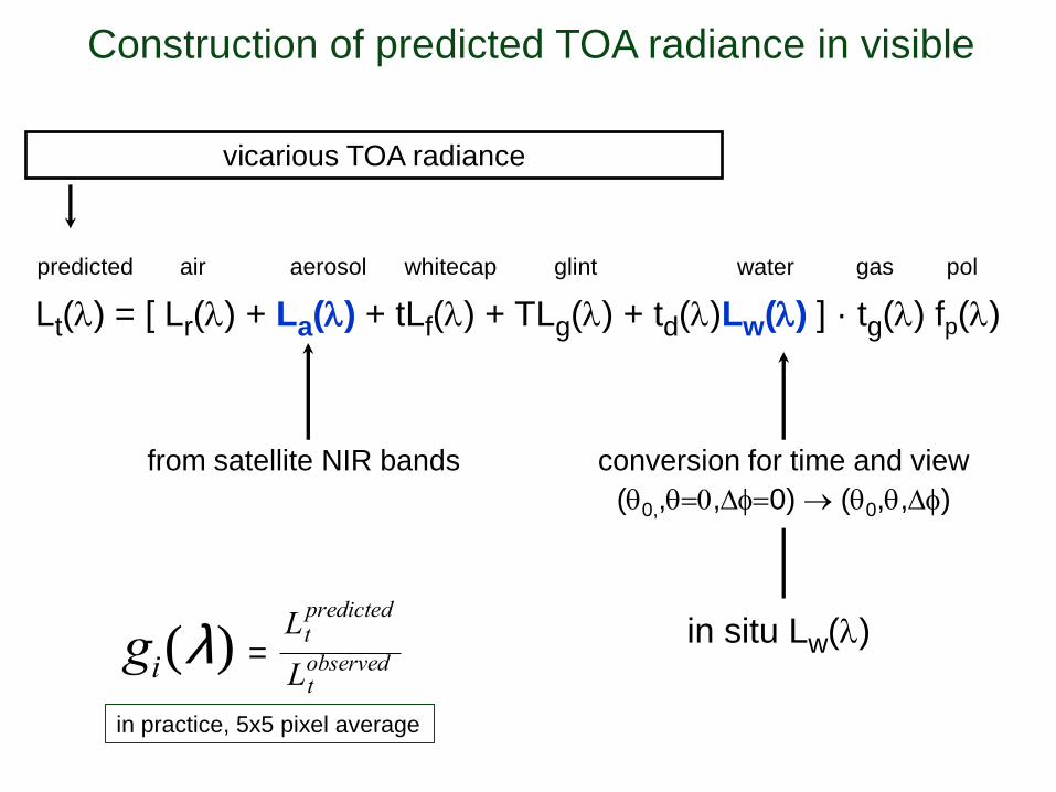
in situ Lw(l)

gas pol glint whitecap air aerosol

Lt(l) = [ Lr(l) + La(l) + tLf(l) + TLg(l) + td(l)Lw(l) ] · tg(l) fp(l)

water

conversion for time and view

(0,,=0,=0) (0,,)

from satellite NIR bands

vicarious TOA radiance

Construction of predicted TOA radiance in visible

predicted

in practice, 5x5 pixel average

 

gi(l) =Ltpredicted

Ltobserved

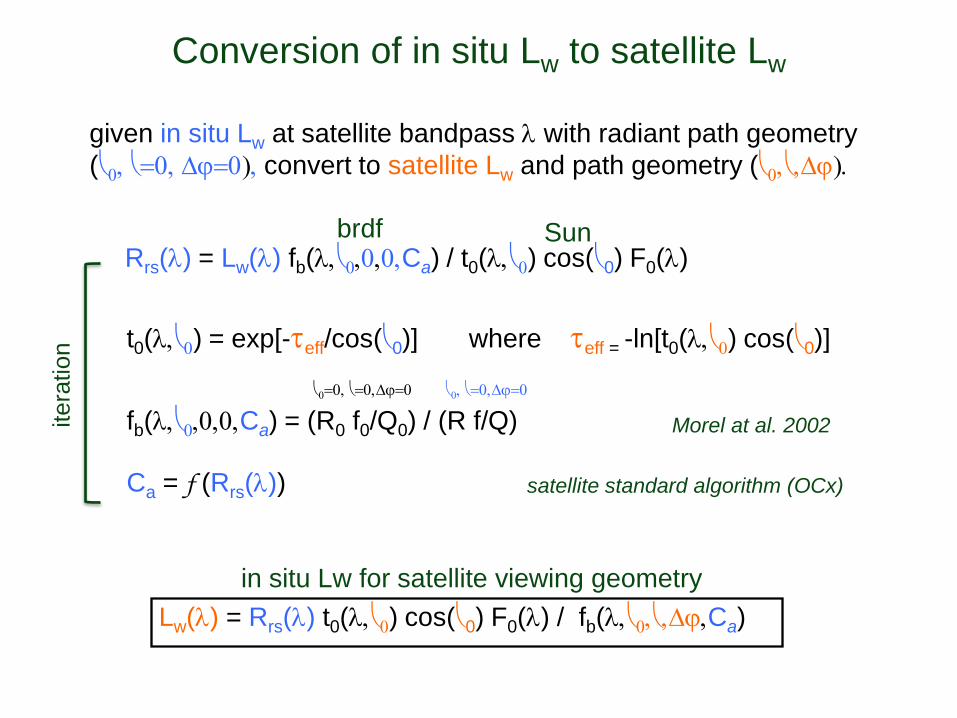
Rrs(l) = Lw(l) fb(l,0,0,0,Ca) / t0(l,0) cos(0) F0(l)

Conversion of in situ Lw to satellite Lw

fb(l,0,0,0,Ca) = (R0 f0/Q0) / (R f/Q)

Ca = f (Rrs(l))

0=0, =0,j=0 0, =0,j=0

t0(l,0) = exp[-teff/cos(0)] where teff = -ln[t0(l,0) cos(0)]

itera

tion

Lw(l) = Rrs(l) t0(l,0) cos(0) F0(l) / fb(l,0,,j,Ca)

given in situ Lw at satellite bandpass l with radiant path geometry

(0, =0, j=0), convert to satellite Lw and path geometry (0,,j).

brdf Sun

Morel at al. 2002

in situ Lw for satellite viewing geometry

satellite standard algorithm (OCx)

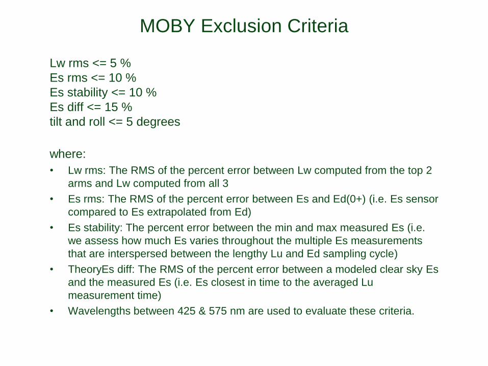
MOBY Exclusion Criteria

Lw rms <= 5 %

Es rms <= 10 %

Es stability <= 10 %

Es diff <= 15 %

tilt and roll <= 5 degrees

where:

• Lw rms: The RMS of the percent error between Lw computed from the top 2

arms and Lw computed from all 3

• Es rms: The RMS of the percent error between Es and Ed(0+) (i.e. Es sensor

compared to Es extrapolated from Ed)

• Es stability: The percent error between the min and max measured Es (i.e.

we assess how much Es varies throughout the multiple Es measurements

that are interspersed between the lengthy Lu and Ed sampling cycle)

• TheoryEs diff: The RMS of the percent error between a modeled clear sky Es

and the measured Es (i.e. Es closest in time to the averaged Lu

measurement time)

• Wavelengths between 425 & 575 nm are used to evaluate these criteria.

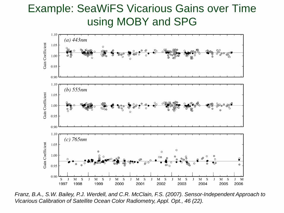
Example: SeaWiFS Vicarious Gains over Time

using MOBY and SPG

Franz, B.A., S.W. Bailey, P.J. Werdell, and C.R. McClain, F.S. (2007). Sensor-Independent Approach to

Vicarious Calibration of Satellite Ocean Color Radiometry, Appl. Opt., 46 (22).

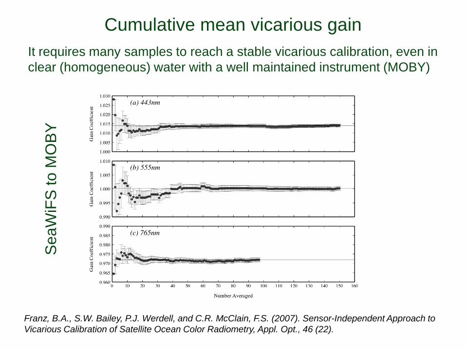
Cumulative mean vicarious gain

It requires many samples to reach a stable vicarious calibration, even in

clear (homogeneous) water with a well maintained instrument (MOBY)

SeaW

iFS

to M

OB

Y

Franz, B.A., S.W. Bailey, P.J. Werdell, and C.R. McClain, F.S. (2007). Sensor-Independent Approach to

Vicarious Calibration of Satellite Ocean Color Radiometry, Appl. Opt., 46 (22).

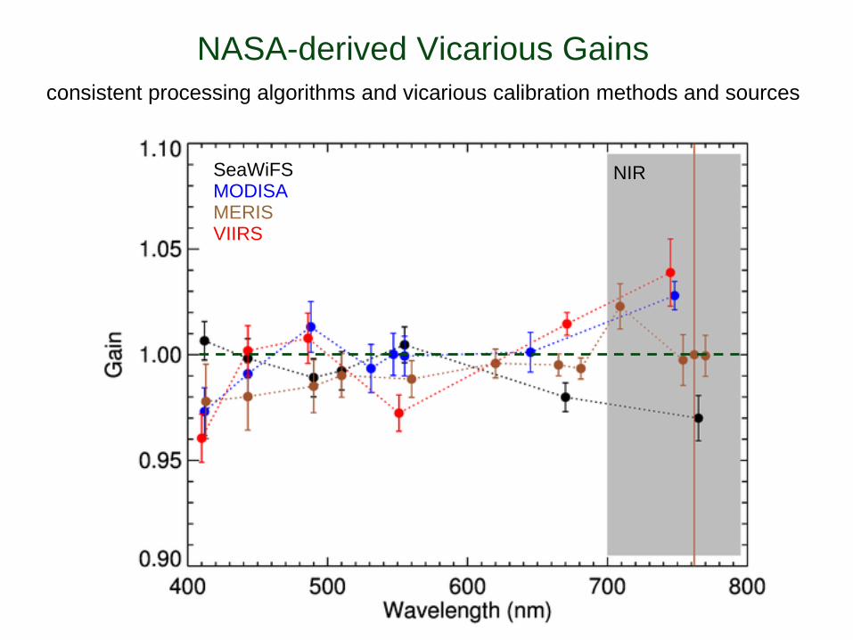
NASA-derived Vicarious Gains

consistent processing algorithms and vicarious calibration methods and sources

SeaWiFS MODISA

VIIRS MERIS

NIR

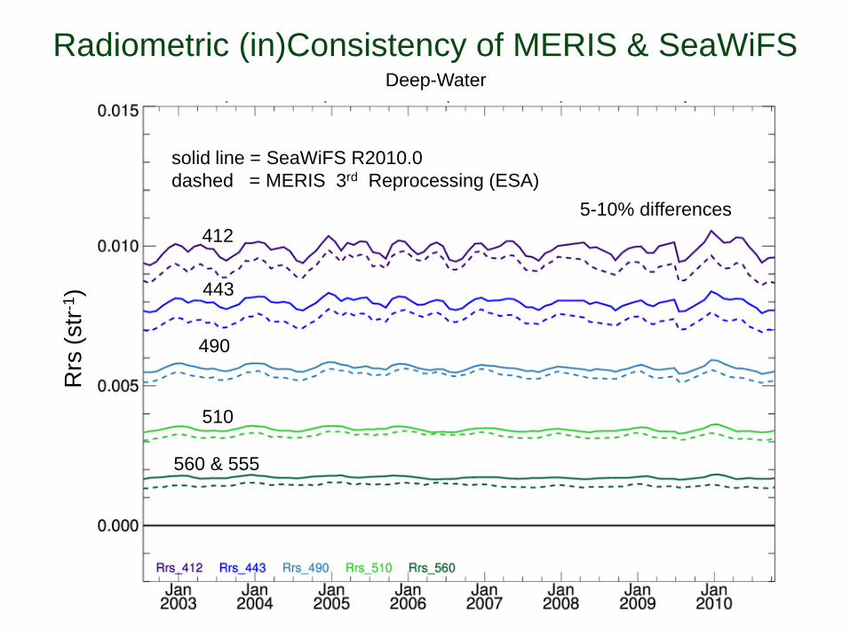
Radiometric (in)Consistency of MERIS & SeaWiFS

412

443

490

510

Deep-Water

solid line = SeaWiFS R2010.0

dashed = MERIS 3rd Reprocessing (ESA)

Rrs

(str

-1)

560 & 555

5-10% differences

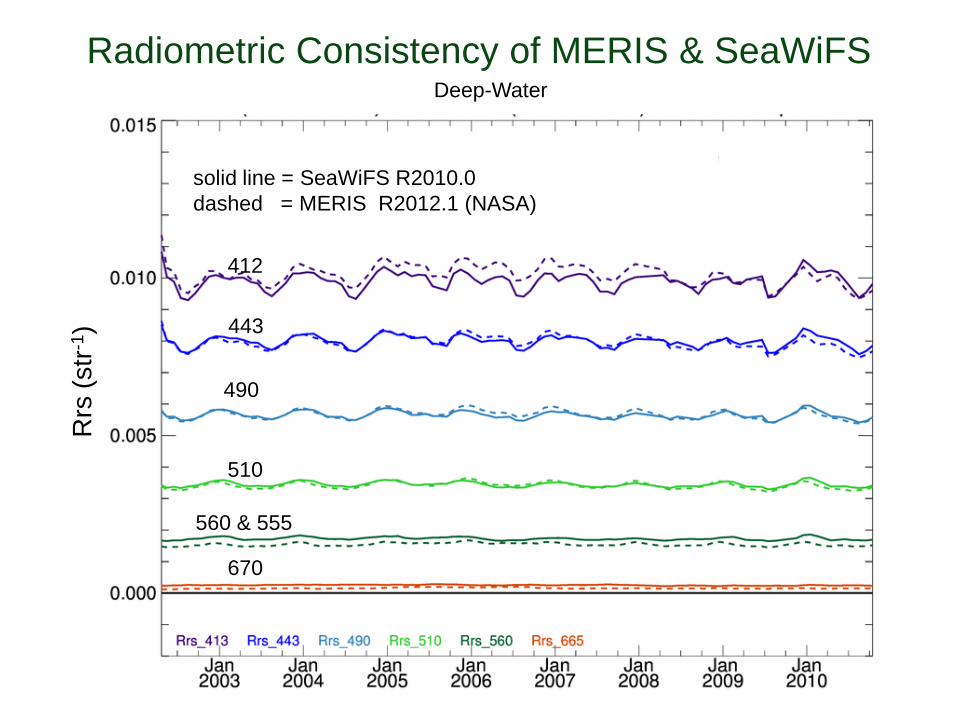
Radiometric Consistency of MERIS & SeaWiFS

412

443

490

510

Deep-Water

solid line = SeaWiFS R2010.0

dashed = MERIS R2012.1 (NASA)

Rrs

(str

-1)

560 & 555

670

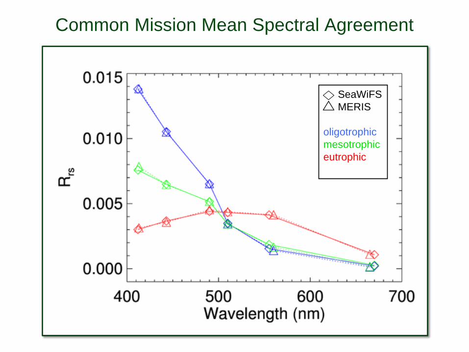
SeaWiFS

MERIS

oligotrophic

mesotrophic

eutrophic

Common Mission Mean Spectral Agreement

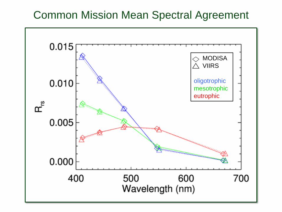
MODISA

VIIRS

oligotrophic

mesotrophic

eutrophic

Common Mission Mean Spectral Agreement

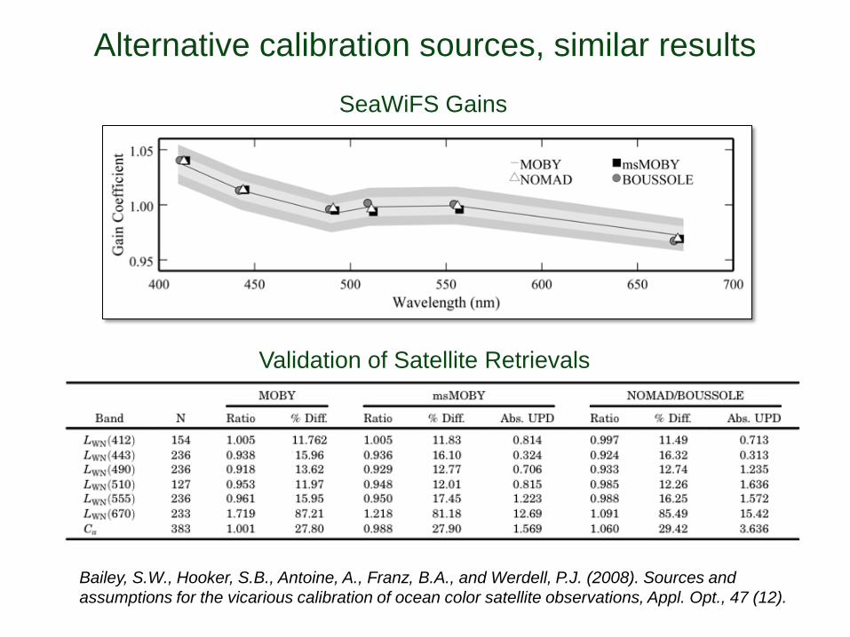
Alternative calibration sources, similar results

SeaWiFS Gains

Validation of Satellite Retrievals

Bailey, S.W., Hooker, S.B., Antoine, A., Franz, B.A., and Werdell, P.J. (2008). Sources and

assumptions for the vicarious calibration of ocean color satellite observations, Appl. Opt., 47 (12).

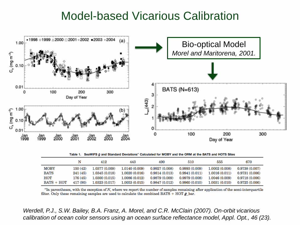
Model-based Vicarious Calibration

Werdell, P.J., S.W. Bailey, B.A. Franz, A. Morel, and C.R. McClain (2007). On-orbit vicarious

calibration of ocean color sensors using an ocean surface reflectance model, Appl. Opt., 46 (23).

Bio-optical Model Morel and Maritorena, 2001.

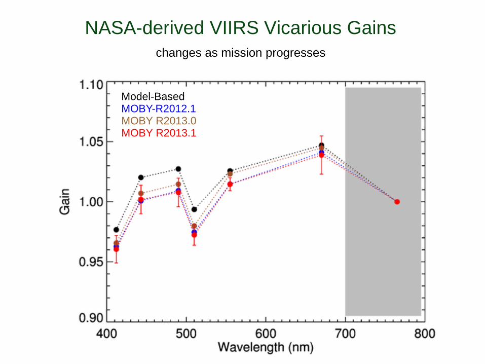
NASA-derived VIIRS Vicarious Gains

changes as mission progresses

Model-Based MOBY-R2012.1

MOBY R2013.1 MOBY R2013.0

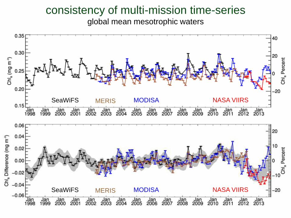
consistency of multi-mission time-series global mean mesotrophic waters

SeaWiFS MODISA NASA VIIRS MERIS

SeaWiFS MODISA NASA VIIRS MERIS

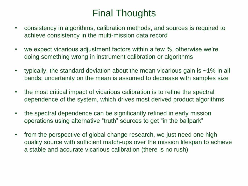
Final Thoughts

• consistency in algorithms, calibration methods, and sources is required to

achieve consistency in the multi-mission data record

• we expect vicarious adjustment factors within a few %, otherwise we’re

doing something wrong in instrument calibration or algorithms

• typically, the standard deviation about the mean vicarious gain is ~1% in all

bands; uncertainty on the mean is assumed to decrease with samples size

• the most critical impact of vicarious calibration is to refine the spectral

dependence of the system, which drives most derived product algorithms

• the spectral dependence can be significantly refined in early mission

operations using alternative “truth” sources to get “in the ballpark”

• from the perspective of global change research, we just need one high

quality source with sufficient match-ups over the mission lifespan to achieve

a stable and accurate vicarious calibration (there is no rush)

22