Embed Size (px)
Citation preview
Nanosurf FlexAFM
Operating Instructions
for
SPM Control SoftwareVersion 3.1

“NANOSURF” AND THE NANOSURF LOGO ARE TRADEMARKS OF NANOSURF AG, REGISTERED AND/OR OTHERWISE PROTECTED IN VARIOUS COUNTRIES.
COPYRIGHT © JULY 2012, NANOSURF AG, SWITZERLAND.OPERATING INSTRUCTIONS V3.1R0, BT03710-15.

Table of contents
PART A: INTRODUCTION TO THE INSTRUMENT
CHAPTER 1: The FlexAFM 151.1: Introduction.............................................................................................. 161.2: Components of the system ...................................................................... 17
1.2.1: Contents of the Tool Set .................................................................................181.3: Connectors, indicators and controls ....................................................... 19
1.3.1: The FlexAFM scan head ..................................................................................191.3.2: The Easyscan 2 Controller ..............................................................................201.3.3: The FlexAFM sample stage............................................................................22
CHAPTER 2: Installing the FlexAFM 232.1: Installing the SPM Control Software....................................................... 24
2.1.1: Preparations before installing ......................................................................242.1.2: Initiating the installation procedure ..........................................................24
2.2: Installing the hardware............................................................................ 252.2.1: Installing the Easyscan 2 controller ............................................................262.2.2: Installing the FlexAFM Video Camera........................................................262.2.3: Installing the Signal Module A .....................................................................282.2.4: Installing the FlexAFM Scan Head ..............................................................28
2.3: Hardware recognition .............................................................................. 30
CHAPTER 3: Preparing for measurement 313.1: Introduction.............................................................................................. 323.2: Initializing the Easyscan 2 Controller ..................................................... 323.3: Installing the cantilever ........................................................................... 33
3.3.1: Selecting a cantilever ......................................................................................343.3.2: Removing the Cantilever Holder.................................................................353.3.3: Inserting the cantilever in the Cantilever Holder ..................................363.3.4: Attaching the Cantilever Holder to the Scan Head ..............................38
3.4: Installing the sample................................................................................ 383.4.1: Preparing the sample ......................................................................................383.4.2: Nanosurf samples .............................................................................................393.4.3: The Sample Stage .............................................................................................423.4.4: Mounting a sample ..........................................................................................44
CHAPTER 4: A first measurement 454.1: Introduction.............................................................................................. 464.2: Running the microscope simulation....................................................... 46
4.2.1: Entering and changing parameter values ...............................................47
Table of contents
4
4.3: Preparing the instrument ........................................................................ 484.4: Approaching the sample ......................................................................... 48
4.4.1: Manual coarse approach using the FlexAFM Sample Stage .............494.4.2: Manual fine approach using the leveling screws..................................514.4.3: Automatic final approach ..............................................................................52
4.5: Starting a measurement .......................................................................... 554.6: Selecting a measurement area................................................................ 564.7: Storing the measurement........................................................................ 574.8: Creating a basic report............................................................................. 584.9: Further options......................................................................................... 58
CHAPTER 5: Improving measurement quality 615.1: Removing interfering signals.................................................................. 62
5.1.1: Mechanical vibrations .....................................................................................625.1.2: Electrical interference......................................................................................625.1.3: Infrared and other light sources ..................................................................63
5.2: Adjusting the measurement plane ......................................................... 635.3: Judging tip quality ................................................................................... 67
CHAPTER 6: Finishing measurements 696.1: Finishing scanning ................................................................................... 706.2: Turning off the instrument ...................................................................... 706.3: Storing the instrument ............................................................................ 71
PART B: SOFTWARE REFERENCE
CHAPTER 7: The user interface 757.1: General concept and layout..................................................................... 767.2: The workspace .......................................................................................... 777.3: Operating windows.................................................................................. 78
7.3.1: Entering and changing parameter values ...............................................797.4: Document space ....................................................................................... 807.5: Panels ........................................................................................................ 817.6: Ribbon ....................................................................................................... 837.7: Status bar .................................................................................................. 847.8: View tab..................................................................................................... 85
7.8.1: Workspace group..............................................................................................857.8.2: Panels group.......................................................................................................857.8.3: Window group ...................................................................................................86
7.9: SPM Parameters dialog............................................................................ 86
5
CHAPTER 8: Operating modes 898.1: Introduction.............................................................................................. 908.2: Acquisition tab ......................................................................................... 90
8.2.1: Preparation group ............................................................................................908.3: Static Force mode ..................................................................................... 938.4: Dynamic Force mode................................................................................ 938.5: Phase Contrast mode ............................................................................... 948.6: Force Modulation mode........................................................................... 968.7: Spreading Resistance mode .................................................................... 978.8: Lateral Force mode................................................................................... 988.9: Kelvin Probe Force Microscopy ............................................................... 98
8.9.1: Introduction........................................................................................................988.9.2: Operating principle..........................................................................................998.9.3: System requirements.......................................................................................998.9.4: Procedures..........................................................................................................101
8.10: Scanning Thermal mode......................................................................... 1108.10.1: SThM measurements......................................................................................1108.10.2: Nano-TA measurements ................................................................................1108.10.3: System requirements and procedures .....................................................111
8.11: SPM Parameters dialog........................................................................... 1138.11.1: Operating Mode page....................................................................................1138.11.2: Z-Controller page.............................................................................................115
8.12: Cantilever Browser dialog ...................................................................... 1178.12.1: Cantilever Editor dialog .................................................................................118
8.13: Vibration Frequency Search dialog ....................................................... 1208.13.1: General concept ...............................................................................................1208.13.2: Automated vibration frequency search...................................................1218.13.3: Manual sweep controls..................................................................................1228.13.4: Auto Frequency Config dialog ....................................................................124
8.14: Laser Alignment dialog........................................................................... 125
CHAPTER 9: Positioning 1279.1: Introduction............................................................................................. 1289.2: Video panel .............................................................................................. 128
9.2.1: Analog video camera display ......................................................................1289.2.2: Digital Video Camera display.......................................................................1299.2.3: Illumination section ........................................................................................1329.2.4: Digital Video Properties dialog ...................................................................133
9.3: Online panel............................................................................................. 1359.3.1: Scan Position section......................................................................................1359.3.2: Master Image section .....................................................................................1369.3.3: Illumination section ........................................................................................136
6
9.4: Stage panel .............................................................................................. 1379.4.1: Move Stage To dialog .....................................................................................138
9.5: Acquisition tab ........................................................................................ 1399.5.1: Approach group ...............................................................................................139
9.6: SPM Parameters dialog........................................................................... 1419.6.1: Approach page .................................................................................................141
9.7: ATS Stage and TSC 3000 driver configuration ...................................... 1439.7.1: Stage Configuration dialog ..........................................................................1459.7.2: The COM Port Configuration dialog..........................................................147
CHAPTER 10: Imaging 14910.1: Introduction............................................................................................. 15010.2: Imaging panel.......................................................................................... 15110.3: The Imaging toolbar................................................................................ 15510.4: Acquisition tab ........................................................................................ 156
10.4.1: Imaging group ..................................................................................................15710.4.2: Scripting group.................................................................................................157
10.5: SPM Parameters dialog........................................................................... 15910.5.1: Imaging page ....................................................................................................159
CHAPTER 11: Spectroscopy 16311.1: Introduction............................................................................................. 16411.2: Spectroscopy Wizard............................................................................... 166
11.2.1: Force–Distance .................................................................................................16711.2.2: Amplitude–Distance / Phase–Distance ...................................................17111.2.3: Tip current–Distance ......................................................................................17311.2.4: Tip current–Tip voltage..................................................................................17411.2.5: User Output Spectroscopy ...........................................................................176
11.3: Spectroscopy panel................................................................................. 17711.4: Spectroscopy toolbar.............................................................................. 17811.5: Acquisition tab ........................................................................................ 180
11.5.1: Spectroscopy group........................................................................................18011.6: SPM Parameters dialog........................................................................... 180
11.6.1: Spectroscopy page..........................................................................................18011.6.2: Spectroscopy page (standard level)..........................................................18111.6.3: Spectroscopy page (advanced level)........................................................184
CHAPTER 12: Lithography 18712.1: Introduction............................................................................................. 18812.2: Performing lithography.......................................................................... 18912.3: Lithography panel................................................................................... 190
12.3.1: Layer Editor dialog...........................................................................................19312.3.2: Object Editor dialog........................................................................................195
7
12.4: Acquisition tab ........................................................................................ 19612.4.1: Lithography group ..........................................................................................196
12.5: Lithography toolbar................................................................................ 19712.5.1: Vector Graphic Import dialog......................................................................19912.5.2: Pixel Graphic Import dialog .........................................................................201
12.6: Lithography preview............................................................................... 20412.7: SPM Parameters dialog........................................................................... 205
12.7.1: Lithography page ............................................................................................205
CHAPTER 13: Working with documents 20713.1: Introduction............................................................................................. 20813.2: Data Info panel ........................................................................................ 208
13.2.1: Data Info toolbar ..............................................................................................20913.3: Charts ....................................................................................................... 209
13.3.1: Working with multiple charts......................................................................21113.3.2: Chart Properties dialog..................................................................................212
13.4: Gallery panel............................................................................................ 21913.4.1: History File mask ..............................................................................................22013.4.2: Image list.............................................................................................................22013.4.3: Gallery toolbar ..................................................................................................22013.4.4: Mask Editor dialog ...........................................................................................22113.4.5: File Rename dialog ..........................................................................................223
13.5: Analysis tab.............................................................................................. 22413.5.1: Measure group..................................................................................................22513.5.2: Correction group..............................................................................................22713.5.3: Roughness group.............................................................................................22913.5.4: Filter group.........................................................................................................23113.5.5: Tools group ........................................................................................................23313.5.6: Report Group.....................................................................................................23413.5.7: Scripting group.................................................................................................236
13.6: Tool panel................................................................................................. 23613.7: File menu.................................................................................................. 238
CHAPTER 14: Options and settings 24114.1: File menu.................................................................................................. 242
14.1.1: Options dialog ..................................................................................................24314.2: Settings tab.............................................................................................. 249
14.2.1: Scan Head group..............................................................................................25014.2.2: Hardware group ...............................................................................................250
14.3: Scan Head Selector dialog ...................................................................... 25114.4: Scan Head Calibration Editor dialog...................................................... 252
14.4.1: Scan Axis .............................................................................................................25214.4.2: I/O Signals...........................................................................................................253
8
14.5: Scan Axis Correction dialog.................................................................... 25514.6: Scan Head Diagnostics dialog ................................................................ 255
14.6.1: Dialog for AFM scan heads ...........................................................................25614.6.2: Dialog for STM scan head .............................................................................256
14.7: Controller Configuration dialog............................................................. 25714.8: SPM Parameters dialog........................................................................... 259
14.8.1: Signal Access page ..........................................................................................25914.8.2: Probe/Tip page .................................................................................................262
14.9: User Signal Editor dialog ........................................................................ 263
CHAPTER 15: Quick reference 265
PART C: APPENDICES
CHAPTER 16: Maintenance 26916.1: Introduction............................................................................................. 27016.2: The FlexAFM scan head........................................................................... 27016.3: The cantilever holder .............................................................................. 27016.4: The Easyscan 2 controller ....................................................................... 270
CHAPTER 17: Problems and solutions 27317.1: Introduction............................................................................................. 27417.2: Software and driver problems ............................................................... 274
17.2.1: No connection to microscope.....................................................................27417.2.2: USB Port error....................................................................................................27417.2.3: Driver problems................................................................................................275
17.3: AFM measurement problems ................................................................. 27717.3.1: Probe Status light blinks red........................................................................27717.3.2: Automatic final approach fails ....................................................................27817.3.3: Image quality suddenly deteriorates........................................................279
17.4: Nanosurf support .................................................................................... 27917.4.1: Self help...............................................................................................................27917.4.2: Assistance ...........................................................................................................280
17.5: About dialog ............................................................................................ 281
CHAPTER 18: AFM theory 28318.1: Scanning probe microscopy ................................................................... 28418.2: The FlexAFM............................................................................................. 285
CHAPTER 19: Technical data 28719.1: Introduction............................................................................................. 288
9
1
19.2: The FlexAFM Scan Head.......................................................................... 28819.2.1: Specifications and features ..........................................................................28819.2.2: Dimensions ........................................................................................................289
19.3: The Easyscan 2 Controller....................................................................... 29119.3.1: Hardware features and specifications ......................................................29119.3.2: Software features and computer requirements ...................................291
19.4: Hardware modules and options............................................................. 29319.4.1: AFM modules ....................................................................................................29319.4.2: Signal Module A ...............................................................................................29419.4.3: The FlexAFM Video Camera .........................................................................29719.4.4: The FlexAFM Micrometer Translation Stage ..........................................297
0

About this Manual
For your convenience, this manual has been divided into three separate parts:
PART A: INTRODUCTION TO THE INSTRUMENT will familiarize you with the Nanosurf FlexAFMsystem, and will explain how to set up your system and operate it on a daily basis. Amongother things, it will also describes how to set up basic experiments and how to generallyimprove measurement quality. Part A starts with Chapter 1: The FlexAFM (page 15) and endswith Chapter 6: Finishing measurements (page 69).
PART B: SOFTWARE REFERENCE is a reference for the software that comes with the FlexAFMsystem. It starts with Chapter 7: The user interface (page 75) and ends with Chapter 15: Quickreference (page 265). Its content applies to Nanosurf Easyscan 2 software version 3.1,Nanosurf Translation Stage Controller software version 2.1, and Nanosurf Batch Mangersoftware version 1.3. If you are using newer software versions, download the latest manualfrom the Nanosurf Support pages or refer to the “What’s new in this version.pdf” file thatcame with the newer software. For more information on the Nanosurf Scripting Interface,refer to the online help files “Easyscan 2 Script Programmers Manual”. For more informationon the Nanosurf Report software, refer to the online help included with this optionalsoftware.
PART C: APPENDICES contains information that you will use less frequently, such as generalmaintenance and troubleshooting. It starts with Chapter 16: Maintenance (page 269) andends with Chapter 19: Technical data (page 287).
11

1
2
PART A:
INTRODUCTION TO THE INSTRUMENT


CHAPTER 1:
The FlexAFM0
0
CHAPTER 1: THE FLEXAFM
1
The Nanosurf FlexAFM system is an atomic force microscope that can measure thetopography and several other properties of a sample with nanometer resolution. Thesemeasurements are performed, displayed, and evaluated using the SPM Control Software.
The FlexAFM system is a modular scanning probe system that can be upgraded to obtainmore measurement capabilities. The main parts of the basic system are the FlexAFM ScanHead, the FlexAFM Sample Stage, the Easyscan 2 Controller with AFM Basic module, andthe SPM Control Software.
The content of the system and the function of its major components are described in thischapter. Detailed technical specifications and system features can be found in Chapter 19:Technical data (page 287).
Several other Nanosurf products can be used in conjunction with the FlexAFM:• AFM Dynamic Module: adds dynamic mode measurement capabilities for measuring
delicate samples.• AFM Mode Extension Module: adds phase contrast, force modulation and current
measurement capabilities.• FlexAFM Video Module: allows observation of the approach on the computer screen.
This is useful when observation using the lenses is impractical.• Signal Module A: allows monitoring of microscope signals and creating custom
operating modes. Refer to Section 19.4.2: Signal Module A (page 294) for more details.• Nanosurf FlexAFM Micrometer Translation Stage: allows locating of a position on a
sample with micrometer accuracy. Should be used together with a FlexAFM SampleStage
• Nanosurf Report: software for simple automatic evaluation and report generation ofSPM measurements.
• Nanosurf Analysis: software for detailed analysis of SPM measurements.• Scripting Interface: software for automating measurements. Refer to Section 10.4.2:
Scripting group (page 157) and the Programmer’s Manual for more details.• Lithography Option: software for professional lithography applications. Refer to Chapter
12: Lithography (page 187) for more information.• The Nanosurf Isostage: a highly compact active vibration isolation table.• The Halcyonics_i4 Active Vibration Isolation Table: a large and heavy-duty active
vibration isolation solution, which features load adjustment.
1.1: Introduction
6
COMPONENTS OF THE SYSTEM
This section describes the parts that may be delivered with an FlexAFM system. Thecontents of delivery can vary from system to system, depending on which parts wereordered. To find out which parts are included in your system, refer to the delivery noteshipped with your system. Some of the modules listed in the delivery note are built into thecontroller. Their presence is indicated by the status lights on the top surface of thecontroller when it is turned on (see Section 1.3.2: The Easyscan 2 Controller (page 20)).
Before unpacking the instrument, verify that the package contains the followingcomponents:
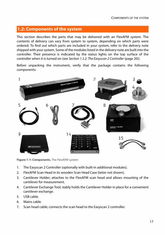
1. The Easyscan 2 Controller (optionally with built-in additional modules). 2. FlexAFM Scan Head in its wooden Scan Head Case (latter not shown).3. Cantilever Holder; attaches to the FlexAFM scan head and allows mounting of the
cantilever for measurement.4. Cantilever Exchange Tool; stably holds the Cantilever Holder in place for a convenient
cantilever exchange.5. USB cable.6. Mains cable. 7. Scan head cable; connects the scan head to the Easyscan 2 controller.
1.2: Components of the system
Figure 1-1: Components. The FlexAFM system
1
8
2
5 6 7
14915
3
4
17
CHAPTER 1: THE FLEXAFM
1
8. FlexAFM Sample Stage (option)9. FlexAFM Tool set (option). The items contained in the FlexAFM Tool set are described
in the next section.10. The Easyscan 2 Installation CD (not shown): Contains software, calibration files, and
PDF files of all manuals.11. A calibration certificate for each scan head (not shown).12. This FlexAFM Operating Instructions manual (not shown).13. AFM Extended Sample Kit (option; not shown), which comes with a set of 10 samples
and description of experiments.14. Signal Module A connector box (option; comes with Signal Module A).15. Two Signal Module cables (option; come with Signal Module A).16. Scripting Interface certificate of purchase with Activation key printed on it (option; not
shown; comes with Scripting Interface).17. Lithography Option certificate of purchase with Activation key printed on it (option;
not shown; comes with the Nanosurf Lithography Option).
Please keep the original packaging material (at least until the end of the warranty period),so that it may be used for transport at a later date, if necessary. For information on how tostore, transport, or send in the instrument for repairs, see Section 6.3: Storing the instrument(page 71).
The content of the Tool set depends on the modules and options included in your order. Itmay contain any of the following items:
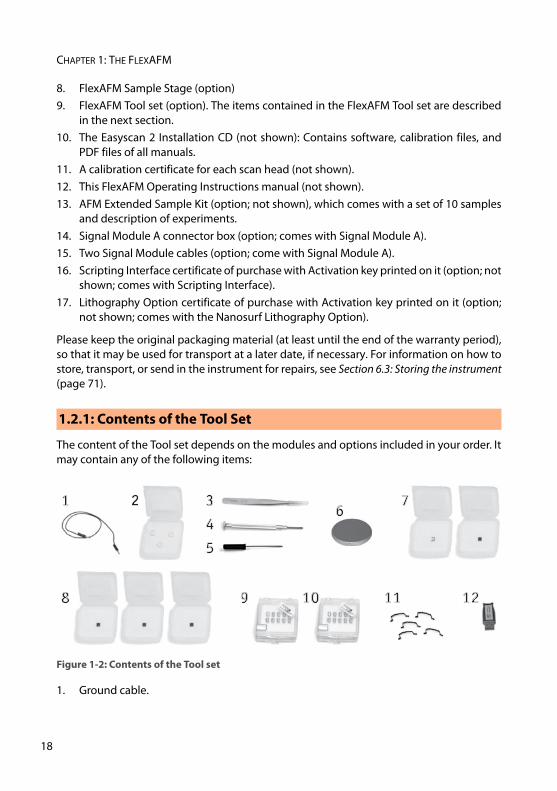
1. Ground cable.
1.2.1: Contents of the Tool Set
Figure 1-2: Contents of the Tool set
12
67
8 9
1 2 345
10 11
8
CONNECTORS, INDICATORS AND CONTROLS
2. Protection feet.3. Cantilever tweezers: (103A CA).4. Screwdriver, 2.3 mm.5. Allen key with screwdriver handle, 1.5 mm (PB-212, ball point hex).6. Sample holder (option; comes with the Flex Sample Stage).7. Samples (option). Possible combinations are:
a. AFM Large Scan Sample Kit (Grid: 10 μm / 100 nm, CD ROM piece).b. AFM High Resolution Sample Kit (Grid: 660 nm, Graphite (HOPG) sample on
sample support).c. Two calibration samples (Calibration grid: 10 μm / 100 nm, Calibration grid:
660 nm).8. AFM Calibration Samples Kit (option) with three calibration samples (Calibration grid:
10 μm / 100 nm, Calibration grid: 660 nm, Flatness sample).9. Set of 10 Static mode cantilevers (option).10. Set of 10 Dynamic mode cantilevers (option).11. Set of 5 cantilever springs.12. USB dongle for Nanosurf Report software (option).
Use this section to find the location of the parts of the FlexAFM that are referred to in thismanual.
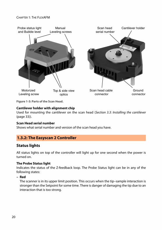
The location of the scan head parts listed below is shown in Figure 1-3: Parts of the ScanHead.
Leveling screwsFor manual fine approach of the sample (Section 4.4.2: Manual fine approach using theleveling screws (page 51)), and for aligning the plane of the scanner with the plane of thesample (Section 5.2: Adjusting the measurement plane (page 63)).
Scan Head cable connectorFor connecting the Scan Head cable that also connects to the Easyscan 2 Controller.
Ground connectorFor connecting a cable that puts the sample or the Sample Holder at the same groundpotential as the scan head.
1.3: Connectors, indicators and controls
1.3.1: The FlexAFM scan head
19
CHAPTER 1: THE FLEXAFM
2
Cantilever holder with alignment chip Used for mounting the cantilever on the scan head (Section 3.3: Installing the cantilever(page 33)).
Scan Head serial numberShows what serial number and version of the scan head you have.
Status lights
All status lights on top of the controller will light up for one second when the power isturned on.
The Probe Status lightIndicates the status of the Z-feedback loop. The Probe Status light can be in any of thefollowing states:– Red
The scanner is in its upper limit position. This occurs when the tip–sample interaction isstronger than the Setpoint for some time. There is danger of damaging the tip due to aninteraction that is too strong.
Figure 1-3: Parts of the Scan Head.
1.3.2: The Easyscan 2 Controller
Scan head cable connector
Motorized Leveling screw
Ground connector
Cantilever holderProbe status lightand Bubble level
Scan head serial number
Manual Leveling screws
Top & side viewoptics
0
CONNECTORS, INDICATORS AND CONTROLS
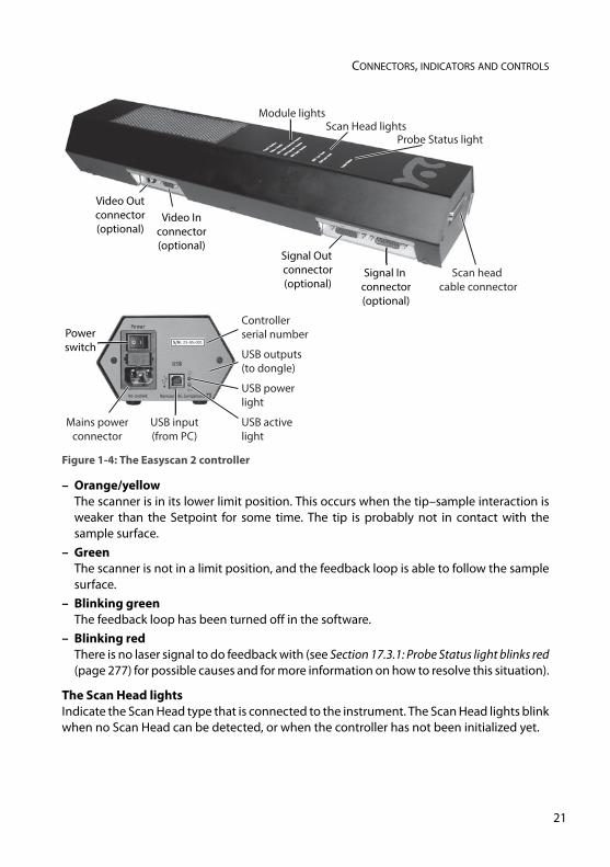
– Orange/yellowThe scanner is in its lower limit position. This occurs when the tip–sample interaction isweaker than the Setpoint for some time. The tip is probably not in contact with thesample surface.
– GreenThe scanner is not in a limit position, and the feedback loop is able to follow the samplesurface.
– Blinking greenThe feedback loop has been turned off in the software.
– Blinking redThere is no laser signal to do feedback with (see Section 17.3.1: Probe Status light blinks red(page 277) for possible causes and for more information on how to resolve this situation).
The Scan Head lightsIndicate the Scan Head type that is connected to the instrument. The Scan Head lights blinkwhen no Scan Head can be detected, or when the controller has not been initialized yet.
Figure 1-4: The Easyscan 2 controller
Video Outconnector(optional)
Probe Status light
Scan head cable connector
Video Inconnector(optional)
Signal Out connector(optional)
Signal In connector(optional)
Scan Head lightsModule lights
Powerswitch
USB activelight
Mains powerconnector
USB powerlight
USB input(from PC)
Controllerserial number
USB outputs(to dongle)
S/N: 23-05-001
21
CHAPTER 1: THE FLEXAFM
2
The Module lightsIndicate the modules that are built in into the controller. The module lights blink when thecontroller has not been initialized yet. During initialization, the module lights are turned onone after the other.
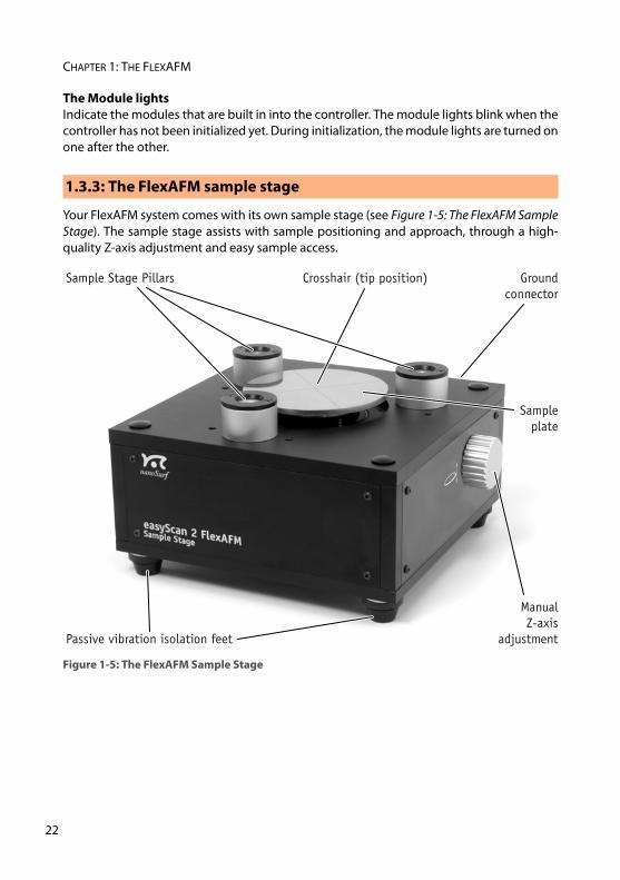
Your FlexAFM system comes with its own sample stage (see Figure 1-5: The FlexAFM SampleStage). The sample stage assists with sample positioning and approach, through a high-quality Z-axis adjustment and easy sample access.
1.3.3: The FlexAFM sample stage
Figure 1-5: The FlexAFM Sample Stage
Sampleplate
ManualZ-axis
adjustment
Sample Stage Pillars Groundconnector
Passive vibration isolation feet
Crosshair (tip position)
2

CHAPTER 2:
Installing the FlexAFM0
0
CHAPTER 2: INSTALLING THE FLEXAFM
2
Before installation, the following steps need to be performed:
1 Make sure the computer to be used meets the minimal computer requirements, asdescribed in Chapter 19: Technical data under Computer requirements (page 292).
2 Make sure none of the FlexAFM system’s hardware is connected to the computer (thisincludes the (USB) FlexAFM Video Camera).
3 Turn on the computer and start Windows.
4 Log on with Administrator privileges.
To initiate the installation procedure:
1 Insert the Easyscan 2 Installation CD into the CD drive of the computer.In most cases, the Autorun CD Menu program will open automatically. Depending onyour Autoplay settings, however, it is also possible that the Autoplay window opens,or that nothing happens at all. In these cases:> Click “Run CD_Start.exe” in the Autoplay window, or manually open the Easyscan
2 Installation CD and start the program “CD_Start.exe”.
2 Click the “Install Easyscan 2 Software” button.The CD Menu program now launches the software setup program, which will startinstallation of all components required to run the Nanosurf Easyscan 2 software. In Windows Vista/7, the User Account Control (UAC) dialog may pop up after clickingthe “Install Easyscan 2 Software” button, displaying the text “An unidentified program
2.1: Installing the SPM Control Software
2.1.1: Preparations before installing
IMPORTANTDo not run any other programs while installing the Easyscan 2 software.
2.1.2: Initiating the installation procedure
IMPORTANTThe Easyscan 2 Installation CD contains calibration information (.hed files) specific toyour instrument! Therefore, always store (a backup copy of ) the CD delivered with theinstrument in a safe place.
4
INSTALLING THE HARDWARE
wants access to your computer”. If the name of the program being displayed is“Setup.exe”:> Click the “Allow” button.
After the software setup program has started:
1 Click “Next” in the “Welcome”, “Select Destination Folder”, and “Select Start MenuFolder” windows that sequentially appear, accepting the default choices in all dialogs.
2 When the “Ready to install” window appears, click on the “Install” button.The setup program now performs its tasks without any further user interaction.Depending on the configuration of your computer, a reboot may be required at theend of the software installation process. If this is the case, the setup program willinform you of this, and will provide you with the opportunity to do so.
This completes the driver and control software installation procedure. If you wish to use theLithography features of the Easyscan 2 software and want to design your own vectorgraphics for import into the lithography module, you can opt to install the LayoutEditorsoftware by clicking the “Install CAD Program” button in the CD Menu program. This willlaunch the LayoutEditor installation program, which will guide you through the CADprogram setup. Otherwise, you may exit now by clicking the “Exit” button and continuewith Section 2.2: Installing the hardware and Section 2.3: Hardware recognition.
2.2: Installing the hardware
IMPORTANT• Make sure that the mains power connection is protected against excess voltage
surges.
• Place the instrument on a stable support in a location that has a low level of buildingvibrations, acoustic noise, electrical fields, and air currents.
IMPORTANT• Never directly touch the cantilevers tips, nor exert too much force on the Cantilever
Deflection System (central part of the disc at the bottom of the Scan Head).
• Ensure that the surface to be measured is free of dust and possible residues.
• Always put the Scan Head in the original packaging material during transport andstorage.
25
CHAPTER 2: INSTALLING THE FLEXAFM
2
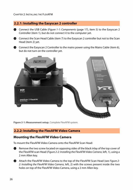
1 Connect the USB Cable (Figure 1-1: Components (page 17), item 5) to the Easyscan 2Controller (item 1), but do not connect it to the computer yet.
2 Connect the Scan Head Cable (item 7) to the Easyscan 2 controller but not to the ScanHead (item 2) yet.
3 Connect the Easyscan 2 Controller to the mains power using the Mains Cable (item 6),but do not turn on the controller yet.
Mounting the FlexAFM Video Camera
To mount the FlexAFM Video Camera onto the FlexAFM Scan Head:
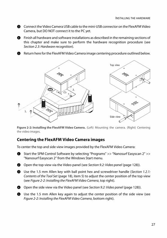
1 Remove the two screw located on opposing sides of the black inlay of the top cover ofthe FlexAFM scan Head (Figure 2-2: Installing the FlexAFM Video Camera, left, 1), using a2 mm Allen key.
2 Attach the FlexAFM Video Camera to the top of the FlexAFM Scan Head (see Figure 2-2: Installing the FlexAFM Video Camera, left, 2) with the screws present inside the twoholes on top of the FlexAFM Video Camera, using a 2 mm Allen key.
2.2.1: Installing the Easyscan 2 controller
Figure 2-1: Measurement setup. Complete FlexAFM system.
2.2.2: Installing the FlexAFM Video Camera
6
INSTALLING THE HARDWARE
3 Connect the Video Camera USB cable to the mini-USB connector on the FlexAFM VideoCamera, but DO NOT connect it to the PC yet.
4 Finish all hardware and software installations as described in the remaining sections ofthis chapter and make sure to perform the hardware recognition procedure (seeSection 2.3: Hardware recognition).
5 Return here for the FlexAFM Video Camera image centering procedure outlined below.
Centering the FlexAFM Video Camera images
To center the top and side view images provided by the FlexAFM Video Camera:
1 Start the SPM Control Software by selecting “Programs” >> “Nanosurf Easyscan 2” >>”Nanosurf Easyscan 2” from the Windows Start menu.
2 Open the top view via the Video panel (see Section 9.2: Video panel (page 128)).
3 Use the 1.5 mm Allen key with ball point hex and screwdriver handle (Section 1.2.1:Contents of the Tool Set (page 18), item 5) to adjust the center position of the top view(see Figure 2-2: Installing the FlexAFM Video Camera, top right).
4 Open the side view via the Video panel (see Section 9.2: Video panel (page 128)).
5 Use the 1.5 mm Allen key again to adjust the center position of the side view (seeFigure 2-2: Installing the FlexAFM Video Camera, bottom right).
Figure 2-2: Installing the FlexAFM Video Camera. (Left) Mounting the camera. (Right) Centeringthe video images.
1.
2.
Side view
Top view
YX
YX
27
CHAPTER 2: INSTALLING THE FLEXAFM
2
To install the Signal Module A:
1 Connect one Signal Module cable (Figure 1-1: Components (page 17), item 15) to theSignal Out connector on the Controller and to the Output connector on the SignalModule A Connector Box.
2 Connect the other Signal Module cable to the Signal In connector on the Controllerand to the Input connector on the Signal Module A Connector Box.
In case of an upgrade, the Easyscan 2 Controller must be sent in to your local Nanosurfdistributor for installation of the Signal Module A electronics in the controller housing.
To mount the Scan Head onto the Sample Stage:
1 Make sure that the height-adjustable Sample Plate with Sample Holder and anyinstalled sample is well below the level where the cantilever will be duringmeasurements.
2 Take the Scan Head in both hands and lower it onto the Sample Stage.The three Leveling Screws should fit stably into the holes of the Sample Stage Pillars.
2.2.3: Installing the Signal Module A
2.2.4: Installing the FlexAFM Scan Head
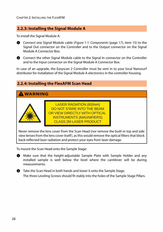
! WARNING
Never remove the lens cover from the Scan Head (nor remove the built-in top and sideview lenses from the lens cover itself ), as this would remove the optical filters that blockback-reflected laser radiation and protect your eyes from laser damage.
LASER RADIATION (650nm)DO NOT STARE INTO THE BEAM
OR VIEW DIRECTLY WITH OPTICAL INSTRUMENTS (MAGNIFIERS)CLASS 2M LASER PRODUCT
8
INSTALLING THE HARDWARE
3 Attach the Scan Head cable (Figure 1-1: Components (page 17), item 7) to the ScanHead (Figure 1-1: Components (page 17), item 2) using the screwdriver (Figure 1-2:Contents of the Tool set (page 18), item 4).
It is recommended to cover the instrument in order to shield it from near-infrared lightfrom artificial light sources, since this light may cause noise in the cantilever deflectiondetection system. The optional Nanosurf Acoustic Enclosures are optimized for this task,and additionally protects against noise and electrical interferences.
If the vibration isolation of your table is insufficient for your measurement purposes, use anactive vibration isolation table such as the Nanosurf Isostage or the Halcyoncis_i4. Refer tothe respective manuals for installation instructions.
-
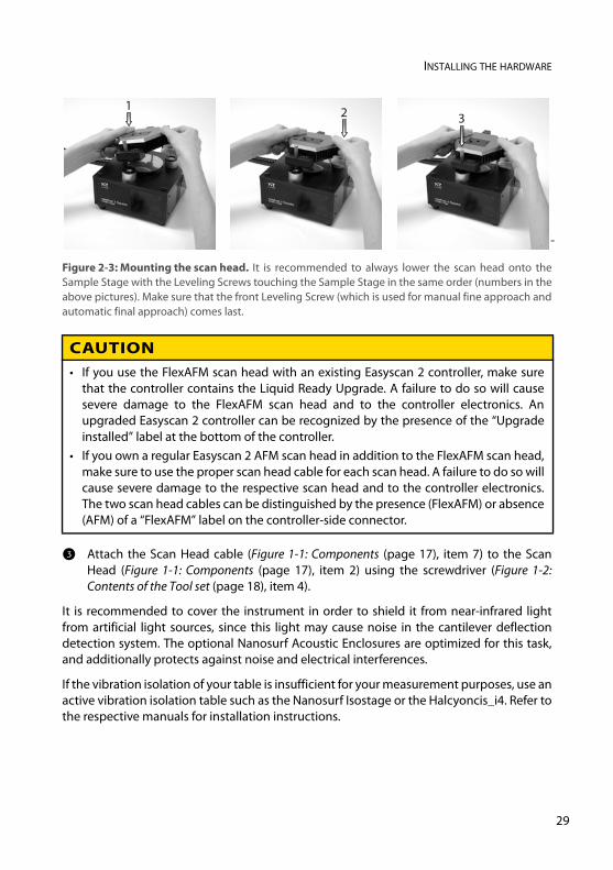
Figure 2-3: Mounting the scan head. It is recommended to always lower the scan head onto theSample Stage with the Leveling Screws touching the Sample Stage in the same order (numbers in theabove pictures). Make sure that the front Leveling Screw (which is used for manual fine approach andautomatic final approach) comes last.
CAUTION• If you use the FlexAFM scan head with an existing Easyscan 2 controller, make sure
that the controller contains the Liquid Ready Upgrade. A failure to do so will causesevere damage to the FlexAFM scan head and to the controller electronics. Anupgraded Easyscan 2 controller can be recognized by the presence of the “Upgradeinstalled” label at the bottom of the controller.
• If you own a regular Easyscan 2 AFM scan head in addition to the FlexAFM scan head,make sure to use the proper scan head cable for each scan head. A failure to do so willcause severe damage to the respective scan head and to the controller electronics.The two scan head cables can be distinguished by the presence (FlexAFM) or absence(AFM) of a “FlexAFM” label on the controller-side connector.
132
29
CHAPTER 2: INSTALLING THE FLEXAFM
3
To initiate the automatic hardware recognition process for the devices present in yoursystem:
1 Install all hardware as described in Section 2.2: Installing the hardware.
2 Power on the Easyscan 2 controller.
3 Connect the Easyscan 2 controller to the computer with the supplied USB cable (Figure1-1: Components (page 17), item 5). If you own a FlexAFM Video Camera, do notconnect it yet.A popup balloon appears in the Windows notification area, stating that new hardwaredevices have been found and drivers are being installed. Depending on theconfiguration of your controller and computer, the detection process can take quitesome time (20 seconds or more). Please be patient! After successful automaticinstallation, the popup balloon indicates that the installation has finished and that thedevices are now ready for use.
4 If you own a FlexAFM Video Camera, it is now time to connect it to a USB port on yourcomputer.On Windows 7 computers, a popup balloon in the Windows notification area maydisplay the message “Problem installing driver”. If this happens:> Disconnect and reconnect the video camera once more.
Hardware recognition will now complete successfully.
5
2.3: Hardware recognition
IMPORTANT• Always connect the FlexAFM Video Camera to a USB port on your personal computer.
The use of USB ports that are mounted directly onto the motherboard (usually locatedat the backside of the PC) is highly recommended. Ports that are not mounted directly(USB ports located at the front of the PC) can cause noise and sync errors due to thesometimes poor quality of cables and connections.
• Do not use the USB hub inside the Easyscan 2 controller (if present), as it does not havesufficient power. The latter will lead to unstable behavior of the video camera and toerratic results.
0

CHAPTER 3:
Preparing for measurement0
0
CHAPTER 3: PREPARING FOR MEASUREMENT
3
Once the system has been set up (see Chapter 2: Installing the FlexAFM (page 23)), theinstrument and the sample have to be prepared for measurement. The preparation consistsof three steps: Initializing the Easyscan 2 Controller, Installing the cantilever, and Installing thesample.
To initialize the Easyscan 2 controller:
1 Make sure that the Easyscan 2 controller is connected to the mains power and to theUSB port of the control computer.
2 Turn on the power of the Easyscan 2 controller.First all status lights on top of the controller briefly light up. Then the Scan Head lightsand the lights of the detected modules will start blinking, and all other status lightsturn off.
3 Start the SPM Control Software on the control computer.The main program window appears, and all status lights are turned off. Now a Message“Controller Startup in progress” is displayed on the computer screen, and the modulelights are turned on one after the other. When initialization is completed, a Message“Starting System” is briefly displayed on the computer screen, and the Probe Statuslight, the Scan Head status light of the detected scan head, and the Module lights ofthe detected modules will light up. If no scan head is detected, both Scan Head Statuslights blink.
4 In the Preparation group of the Acquisition tab you will see the currently selectedMeasurement environment, Operating mode and Cantilever type.
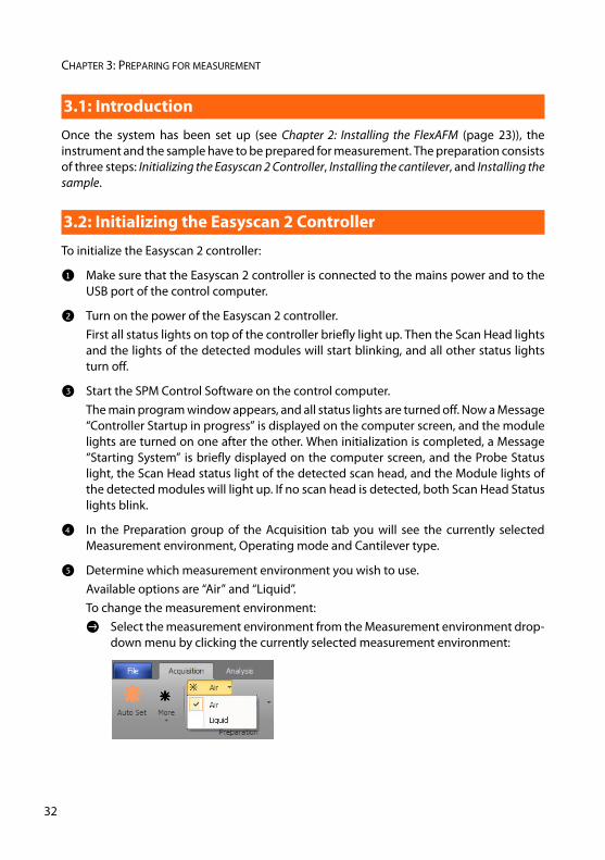
5 Determine which measurement environment you wish to use.Available options are “Air” and “Liquid”. To change the measurement environment:> Select the measurement environment from the Measurement environment drop-
down menu by clicking the currently selected measurement environment:
3.1: Introduction
3.2: Initializing the Easyscan 2 Controller
2
INSTALLING THE CANTILEVER
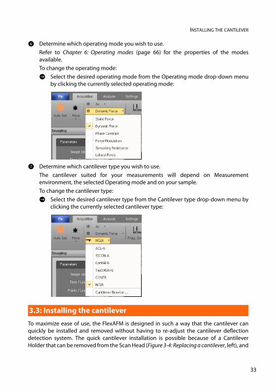
6 Determine which operating mode you wish to use.Refer to Chapter 6: Operating modes (page 66) for the properties of the modesavailable.To change the operating mode:> Select the desired operating mode from the Operating mode drop-down menu
by clicking the currently selected operating mode:
7 Determine which cantilever type you wish to use.The cantilever suited for your measurements will depend on Measurementenvironment, the selected Operating mode and on your sample.To change the cantilever type:> Select the desired cantilever type from the Cantilever type drop-down menu by
clicking the currently selected cantilever type:
To maximize ease of use, the FlexAFM is designed in such a way that the cantilever canquickly be installed and removed without having to re-adjust the cantilever deflectiondetection system. The quick cantilever installation is possible because of a CantileverHolder that can be removed from the Scan Head (Figure 3-4: Replacing a cantilever, left), and
3.3: Installing the cantilever
33
CHAPTER 3: PREPARING FOR MEASUREMENT
3
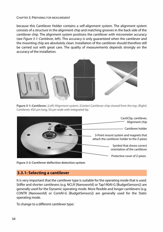
because this Cantilever Holder contains a self-alignment system. The alignment systemconsists of a structure in the alignment chip and matching grooves in the back side of thecantilever chip. The alignment system positions the cantilever with micrometer accuracy(see Figure 3-1: Cantilever, left). This accuracy is only guaranteed when the cantilever andthe mounting chip are absolutely clean. Installation of the cantilever should therefore stillbe carried out with great care. The quality of measurements depends strongly on theaccuracy of the installation.
It is very important that the cantilever type is suitable for the operating mode that is used.Stiffer and shorter cantilevers (e.g. NCLR [Nanoworld] or Tap190Al-G [BudgetSensors]) aregenerally used for the Dynamic operating mode. More flexible and longer cantilevers (e.g.CONTR [Nanoworld] or ContAl-G [BudgetSensors]) are generally used for the Staticoperating mode.
To change to a different cantilever type:
Figure 3-1: Cantilever. (Left) Alignment system. (Center) Cantilever chip viewed from the top. (Right)Cantilever, 450 μm long, 50 μm wide with integrated tip.
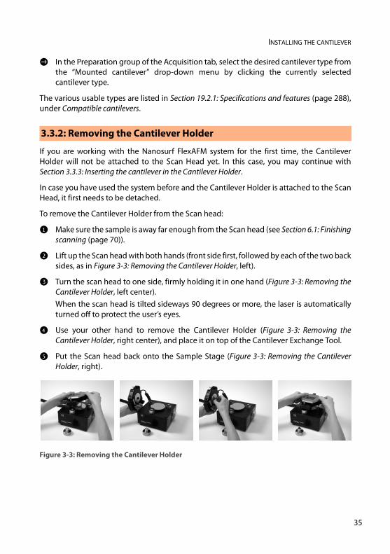
Figure 3-2: Cantilever deflection detection system
3.3.1: Selecting a cantilever
Protective cover of Z-piezo
Symbol that shows correct orientation of the cantilever
Cantilever holder
CantiClip, cantilever,Alignment chip
3-Point mount system and magnets thatattach the cantilever holder to the Z-piezo
4
INSTALLING THE CANTILEVER
> In the Preparation group of the Acquisition tab, select the desired cantilever type fromthe “Mounted cantilever” drop-down menu by clicking the currently selectedcantilever type.
The various usable types are listed in Section 19.2.1: Specifications and features (page 288),under Compatible cantilevers.
If you are working with the Nanosurf FlexAFM system for the first time, the CantileverHolder will not be attached to the Scan Head yet. In this case, you may continue withSection 3.3.3: Inserting the cantilever in the Cantilever Holder.
In case you have used the system before and the Cantilever Holder is attached to the ScanHead, it first needs to be detached.
To remove the Cantilever Holder from the Scan head:
1 Make sure the sample is away far enough from the Scan head (see Section 6.1: Finishingscanning (page 70)).
2 Lift up the Scan head with both hands (front side first, followed by each of the two backsides, as in Figure 3-3: Removing the Cantilever Holder, left).
3 Turn the scan head to one side, firmly holding it in one hand (Figure 3-3: Removing theCantilever Holder, left center).When the scan head is tilted sideways 90 degrees or more, the laser is automaticallyturned off to protect the user’s eyes.
4 Use your other hand to remove the Cantilever Holder (Figure 3-3: Removing theCantilever Holder, right center), and place it on top of the Cantilever Exchange Tool.
5 Put the Scan head back onto the Sample Stage (Figure 3-3: Removing the CantileverHolder, right).
3.3.2: Removing the Cantilever Holder
Figure 3-3: Removing the Cantilever Holder
35
CHAPTER 3: PREPARING FOR MEASUREMENT
3
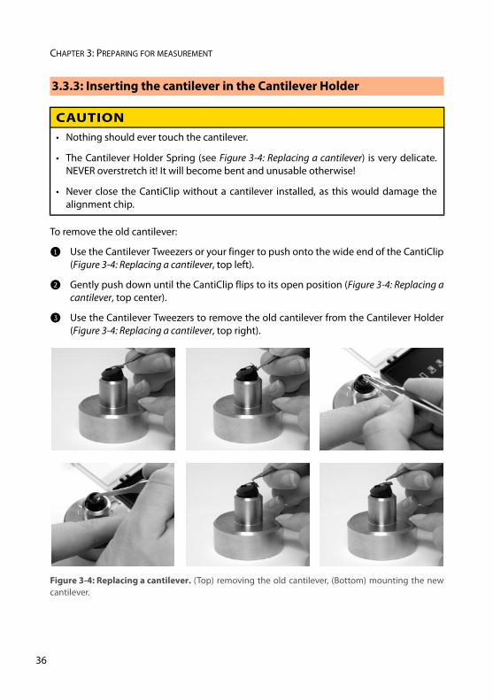
To remove the old cantilever:
1 Use the Cantilever Tweezers or your finger to push onto the wide end of the CantiClip(Figure 3-4: Replacing a cantilever, top left).
2 Gently push down until the CantiClip flips to its open position (Figure 3-4: Replacing acantilever, top center).
3 Use the Cantilever Tweezers to remove the old cantilever from the Cantilever Holder(Figure 3-4: Replacing a cantilever, top right).
3.3.3: Inserting the cantilever in the Cantilever Holder
CAUTION• Nothing should ever touch the cantilever.
• The Cantilever Holder Spring (see Figure 3-4: Replacing a cantilever) is very delicate.NEVER overstretch it! It will become bent and unusable otherwise!
• Never close the CantiClip without a cantilever installed, as this would damage thealignment chip.
Figure 3-4: Replacing a cantilever. (Top) removing the old cantilever, (Bottom) mounting the newcantilever.
6
INSTALLING THE CANTILEVER
In case the previous measurement was performed in liquid (Cantilever Holder Liquid/Air),the cantilever (if it is to be re-used) and the Cantilever Holder need to be cleaned first. Todo this:
1 Carefully remove most excess liquid from the cantilever and Cantilever Holder with apiece of paper.If the Cantilever Alignment Chip is really dirty, you can clean it with mild dish soap,followed by rinsing with clean water.
2 Use a (compressed gas) air duster to blow-dry the cantilever and Cantilever Holder.
To insert the new cantilever:
1 Take the new cantilever out of its box with the cantilever tweezers.
2 Place the cantilever carefully on the alignment chip (Figure 3-4: Replacing a cantilever,top right).
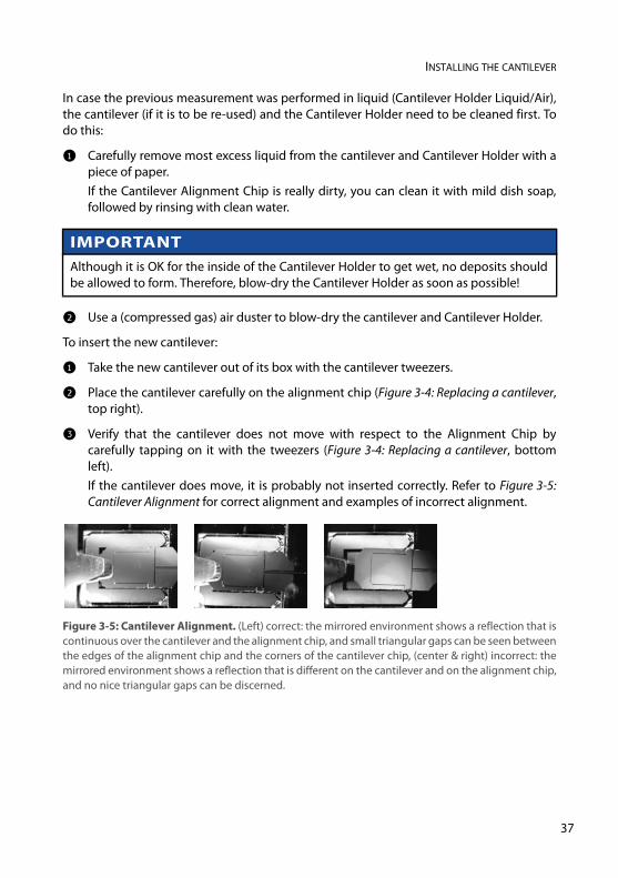
3 Verify that the cantilever does not move with respect to the Alignment Chip bycarefully tapping on it with the tweezers (Figure 3-4: Replacing a cantilever, bottomleft).If the cantilever does move, it is probably not inserted correctly. Refer to Figure 3-5:Cantilever Alignment for correct alignment and examples of incorrect alignment.
IMPORTANTAlthough it is OK for the inside of the Cantilever Holder to get wet, no deposits shouldbe allowed to form. Therefore, blow-dry the Cantilever Holder as soon as possible!
Figure 3-5: Cantilever Alignment. (Left) correct: the mirrored environment shows a reflection that iscontinuous over the cantilever and the alignment chip, and small triangular gaps can be seen betweenthe edges of the alignment chip and the corners of the cantilever chip, (center & right) incorrect: themirrored environment shows a reflection that is different on the cantilever and on the alignment chip,and no nice triangular gaps can be discerned.
37
CHAPTER 3: PREPARING FOR MEASUREMENT
3
4 Use the cantilever tweezers or your finger to gently push on the narrow end of theCantiClip (Figure 3-4: Replacing a cantilever, bottom center image).The CantiClip snaps into its closed position and firmly holds the cantliever in place (seeFigure 3-4: Replacing a cantilever, bottom right). The cantilever is now securely attachedand aligned.
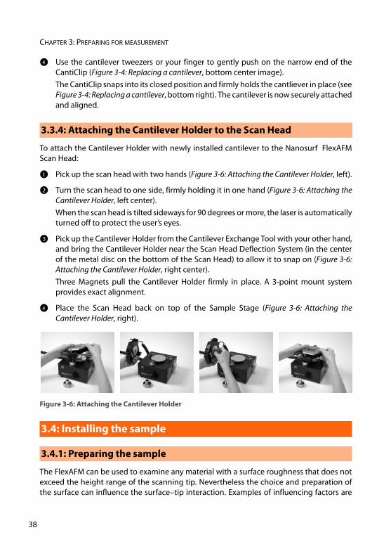
To attach the Cantilever Holder with newly installed cantilever to the Nanosurf FlexAFMScan Head:
1 Pick up the scan head with two hands (Figure 3-6: Attaching the Cantilever Holder, left).
2 Turn the scan head to one side, firmly holding it in one hand (Figure 3-6: Attaching theCantilever Holder, left center). When the scan head is tilted sideways for 90 degrees or more, the laser is automaticallyturned off to protect the user’s eyes.
3 Pick up the Cantilever Holder from the Cantilever Exchange Tool with your other hand,and bring the Cantilever Holder near the Scan Head Deflection System (in the centerof the metal disc on the bottom of the Scan Head) to allow it to snap on (Figure 3-6:Attaching the Cantilever Holder, right center). Three Magnets pull the Cantilever Holder firmly in place. A 3-point mount systemprovides exact alignment.
4 Place the Scan Head back on top of the Sample Stage (Figure 3-6: Attaching theCantilever Holder, right).
The FlexAFM can be used to examine any material with a surface roughness that does notexceed the height range of the scanning tip. Nevertheless the choice and preparation ofthe surface can influence the surface–tip interaction. Examples of influencing factors are
3.3.4: Attaching the Cantilever Holder to the Scan Head
Figure 3-6: Attaching the Cantilever Holder
3.4: Installing the sample
3.4.1: Preparing the sample
8
INSTALLING THE SAMPLE
excess moisture (during measurements in air), dust, grease or other contaminations of thesample surface. Because of this, some samples need special preparation to clean theirsurface. Generally, however, only clean your samples if this is absolutely required, and besure to clean very carefully in order not to harm the sample surface. Some contaminationsmay go away without any further cleaning when performing measurements in liquid. Youmay consider trying this instead of cleaning.
If the surface is dusty, try to measure on a clean area between the dust. Although it ispossible to blow away coarse particles with dry, oil-free air, small particles generally stickquite strongly to the surface and cannot be easily removed this way. Also note that bottled,pressurized air is generally dry, but pressurized air from an in-house supply is generally not.In this case an oil filter should be installed. Blowing away dust by breath is not advisable,because the risk of contaminating the sample even further is very high.
When the sample surface is contaminated with solid matter or substances that can bedissolved, the surface should be cleaned with a solvent. Suitable solvents are distilled ordemineralized water, alcohol or acetone, depending on the nature of the contaminant. Thesolvent should always be highly pure in order to prevent accumulation of impuritiescontained within the solvent on the sample surface. When the sample is very dirty, it shouldbe cleaned several times to completely remove partially dissolved and redepositedcontaminants. Delicate samples, which would suffer from such a treatment, canalternatively be cleaned in an ultrasonic bath.
Nanosurf delivers various optional samples, which are usually packed in the FlexAFM ToolSet. These samples are briefly described here. Further samples are available in the AFMExtended Sample Kit, which contains its own sample description.
All samples should be stored in their respective box. This way, it should not be necessary toclean them. Cleaning of the samples is generally not advisable (unless indicated below),because their surfaces are often rather delicate.
3.4.2: Nanosurf samples
39
CHAPTER 3: PREPARING FOR MEASUREMENT
4
Grid: 10 μm / 100 nm
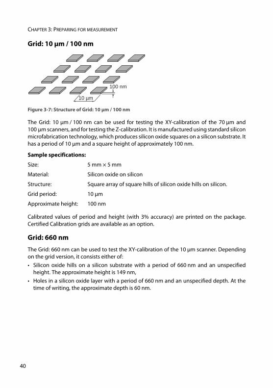
The Grid: 10 μm / 100 nm can be used for testing the XY-calibration of the 70 μm and100 μm scanners, and for testing the Z-calibration. It is manufactured using standard siliconmicrofabrication technology, which produces silicon oxide squares on a silicon substrate. Ithas a period of 10 μm and a square height of approximately 100 nm.
Sample specifications:
Calibrated values of period and height (with 3% accuracy) are printed on the package.Certified Calibration grids are available as an option.
Grid: 660 nm
The Grid: 660 nm can be used to test the XY-calibration of the 10 μm scanner. Dependingon the grid version, it consists either of:• Silicon oxide hills on a silicon substrate with a period of 660 nm and an unspecified
height. The approximate height is 149 nm,• Holes in a silicon oxide layer with a period of 660 nm and an unspecified depth. At the
time of writing, the approximate depth is 60 nm.
Figure 3-7: Structure of Grid: 10 μm / 100 nm
Size: 5 mm × 5 mm
Material: Silicon oxide on silicon
Structure: Square array of square hills of silicon oxide hills on silicon.
Grid period: 10 μm
Approximate height: 100 nm
100 nm
10 µm
0
INSTALLING THE SAMPLE
Sample specifications:
Flatness sample
The Flatness sample is a polished silicon sample. It can be used for testing the Flatness ofthe scanned plane.
Sample specifications:
CD-ROM piece
Sample for demonstrating the AFM imaging. The CD sample is a piece from a CD, withoutany coating applied to it.
Sample specifications:
Microstructure
Sample for demonstrating AFM imaging (no longer available). The microstructure isapproximately the negative of the Grid: 10μm / 100nm. It consists of holes in a silicon oxide
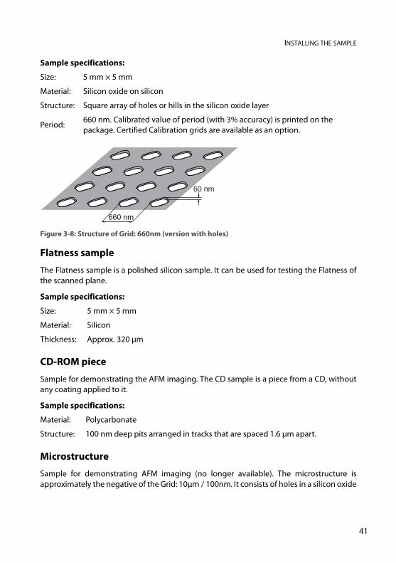
Figure 3-8: Structure of Grid: 660nm (version with holes)
Size: 5 mm × 5 mm
Material: Silicon oxide on silicon
Structure: Square array of holes or hills in the silicon oxide layer
Period:660 nm. Calibrated value of period (with 3% accuracy) is printed on the package. Certified Calibration grids are available as an option.
Size: 5 mm × 5 mm
Material: Silicon
Thickness: Approx. 320 μm
Material: Polycarbonate
Structure: 100 nm deep pits arranged in tracks that are spaced 1.6 μm apart.
660 nm
60 nm
41
CHAPTER 3: PREPARING FOR MEASUREMENT
4
layer with an unspecified period and depth. The approximate period is 10 μm, theapproximate depth is 100 nm.
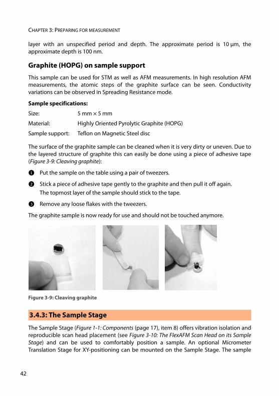
Graphite (HOPG) on sample support
This sample can be used for STM as well as AFM measurements. In high resolution AFMmeasurements, the atomic steps of the graphite surface can be seen. Conductivityvariations can be observed in Spreading Resistance mode.
Sample specifications:
The surface of the graphite sample can be cleaned when it is very dirty or uneven. Due tothe layered structure of graphite this can easily be done using a piece of adhesive tape(Figure 3-9: Cleaving graphite):
1 Put the sample on the table using a pair of tweezers.
2 Stick a piece of adhesive tape gently to the graphite and then pull it off again.The topmost layer of the sample should stick to the tape.
3 Remove any loose flakes with the tweezers.
The graphite sample is now ready for use and should not be touched anymore.
The Sample Stage (Figure 1-1: Components (page 17), item 8) offers vibration isolation andreproducible scan head placement (see Figure 3-10: The FlexAFM Scan Head on its SampleStage) and can be used to comfortably position a sample. An optional MicrometerTranslation Stage for XY-positioning can be mounted on the Sample Stage. The sample
Size: 5 mm × 5 mm
Material: Highly Oriented Pyrolytic Graphite (HOPG)
Sample support: Teflon on Magnetic Steel disc
Figure 3-9: Cleaving graphite
3.4.3: The Sample Stage
2
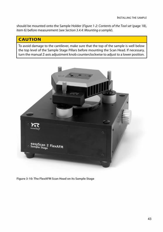
INSTALLING THE SAMPLE
should be mounted onto the Sample Holder (Figure 1-2: Contents of the Tool set (page 18),item 6) before measurement (see Section 3.4.4: Mounting a sample).
CAUTIONTo avoid damage to the cantilever, make sure that the top of the sample is well belowthe top level of the Sample Stage Pillars before mounting the Scan Head. If necessary,turn the manual Z-axis adjustment knob counterclockwise to adjust to a lower position.
Figure 3-10: The FlexAFM Scan Head on its Sample Stage
43
CHAPTER 3: PREPARING FOR MEASUREMENT
4
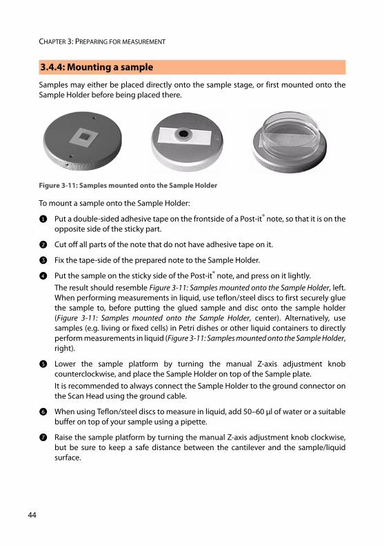
Samples may either be placed directly onto the sample stage, or first mounted onto theSample Holder before being placed there.
To mount a sample onto the Sample Holder:
1 Put a double-sided adhesive tape on the frontside of a Post-it® note, so that it is on theopposite side of the sticky part.
2 Cut off all parts of the note that do not have adhesive tape on it.
3 Fix the tape-side of the prepared note to the Sample Holder.
4 Put the sample on the sticky side of the Post-it® note, and press on it lightly.The result should resemble Figure 3-11: Samples mounted onto the Sample Holder, left.When performing measurements in liquid, use teflon/steel discs to first securely gluethe sample to, before putting the glued sample and disc onto the sample holder(Figure 3-11: Samples mounted onto the Sample Holder, center). Alternatively, usesamples (e.g. living or fixed cells) in Petri dishes or other liquid containers to directlyperform measurements in liquid (Figure 3-11: Samples mounted onto the Sample Holder,right).
5 Lower the sample platform by turning the manual Z-axis adjustment knobcounterclockwise, and place the Sample Holder on top of the Sample plate.It is recommended to always connect the Sample Holder to the ground connector onthe Scan Head using the ground cable.
6 When using Teflon/steel discs to measure in liquid, add 50–60 μl of water or a suitablebuffer on top of your sample using a pipette.
7 Raise the sample platform by turning the manual Z-axis adjustment knob clockwise,but be sure to keep a safe distance between the cantilever and the sample/liquidsurface.
3.4.4: Mounting a sample
Figure 3-11: Samples mounted onto the Sample Holder
4

CHAPTER 4:
A first measurement0
0
CHAPTER 4: A FIRST MEASUREMENT
4
In this chapter, step-by-step instructions are given to operate the microscope and toperform a simple measurement in air and in liquid. More detailed explanations of thesoftware and of the system can be found elsewhere in this manual.
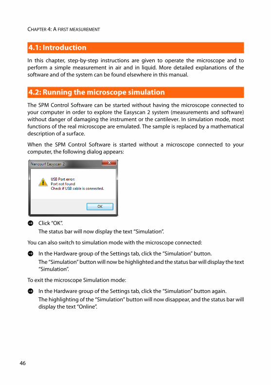
The SPM Control Software can be started without having the microscope connected toyour computer in order to explore the Easyscan 2 system (measurements and software)without danger of damaging the instrument or the cantilever. In simulation mode, mostfunctions of the real microscope are emulated. The sample is replaced by a mathematicaldescription of a surface.
When the SPM Control Software is started without a microscope connected to yourcomputer, the following dialog appears:
> Click “OK”.The status bar will now display the text “Simulation”.
You can also switch to simulation mode with the microscope connected:
> In the Hardware group of the Settings tab, click the “Simulation” button.The “Simulation” button will now be highlighted and the status bar will display the text“Simulation”.
To exit the microscope Simulation mode:
> In the Hardware group of the Settings tab, click the “Simulation” button again.The highlighting of the “Simulation” button will now disappear, and the status bar willdisplay the text “Online”.
4.1: Introduction
4.2: Running the microscope simulation
6
RUNNING THE MICROSCOPE SIMULATION
When using the Nanosurf FlexAFM and SPM control software, you may from time to timeneed to change or enter parameter values. These can be found in the parameter sectionsof the Operating windows and in various dialogs.
To change a parameter or enter a value:
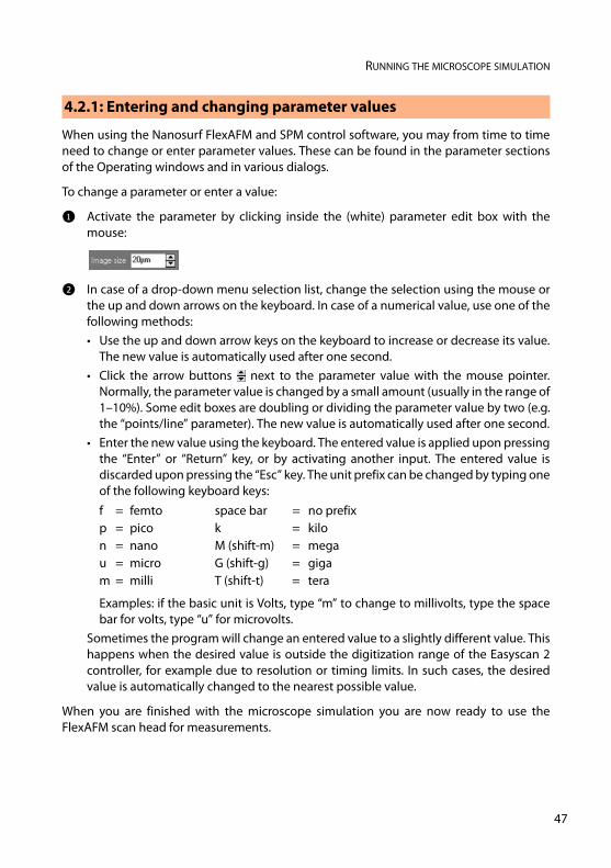
1 Activate the parameter by clicking inside the (white) parameter edit box with themouse:
2 In case of a drop-down menu selection list, change the selection using the mouse orthe up and down arrows on the keyboard. In case of a numerical value, use one of thefollowing methods:• Use the up and down arrow keys on the keyboard to increase or decrease its value.
The new value is automatically used after one second.• Click the arrow buttons next to the parameter value with the mouse pointer.
Normally, the parameter value is changed by a small amount (usually in the range of1–10%). Some edit boxes are doubling or dividing the parameter value by two (e.g.the “points/line” parameter). The new value is automatically used after one second.
• Enter the new value using the keyboard. The entered value is applied upon pressingthe “Enter” or “Return” key, or by activating another input. The entered value isdiscarded upon pressing the “Esc” key. The unit prefix can be changed by typing oneof the following keyboard keys:
Examples: if the basic unit is Volts, type “m” to change to millivolts, type the spacebar for volts, type “u” for microvolts.
Sometimes the program will change an entered value to a slightly different value. Thishappens when the desired value is outside the digitization range of the Easyscan 2controller, for example due to resolution or timing limits. In such cases, the desiredvalue is automatically changed to the nearest possible value.
When you are finished with the microscope simulation you are now ready to use theFlexAFM scan head for measurements.
4.2.1: Entering and changing parameter values
f = femto space bar = no prefixp = pico k = kilon = nano M (shift-m) = megau = micro G (shift-g) = gigam = milli T (shift-t) = tera
47
CHAPTER 4: A FIRST MEASUREMENT
4
Prepare the instrument as follows (see Chapter 3: Preparing for measurement (page 31) formore detailed instructions):
1 If your Easyscan 2 Controller has Dynamic measurement capabilities, install an NCLRtype cantilever. Otherwise install a CONTR type cantilever.
2 Install one of the samples from the Nanosurf AFM Basic Sample Kit or CalibrationSample Kit. Preferably, install the 10 μm Calibration grid.The measurement examples shown here were made with the 10 μm Calibration grid.
To make sure that the configuration is correct, do the following:
> Open the menu item “File” >> “Parameters” >> “Load...” and load the file“Default_FlexAFM.par” from the directory that holds the default Easyscan 2configurations. Usually this is “C:\Program Files\Nanosurf\Nansurf Easyscan 2\Config”.
To start measuring, the cantilever tip must come within a fraction of a nanometer of thesample without touching it with too much force. To achieve this, a very careful and sensitiveapproach of the cantilever is required. This delicate operation is carried out in three steps:Manual coarse approach using the FlexAFM Sample Stage, Manual fine approach using theleveling screws, and the Automatic final approach. The color of the Status lights on thecontroller and on the scan head show the current status of the approach:– Orange/yellow
Normal state during approach: the Z-scanner is fully extended toward the sample.– Red
The approach has gone too far: the tip was driven into the sample, and the Z-scanner isfully retracted from the sample. In this case, the tip is probably damaged and you willhave to install a new cantilever again.
– GreenThe approach has finished successfully: the Z-scanner is within the measuring range.
4.3: Preparing the instrument
IMPORTANT• Never touch the cantilever or the surface of the sample! Good results rely heavily on a
correct treatment of the tip and the sample.
• Avoid exposing the system to direct light while measuring. This could influence thecantilever deflection detection system and reduce the quality of the measurement.
4.4: Approaching the sample
8
APPROACHING THE SAMPLE
To prepare for the approach process:
1 Select the Acquisition tab.The controls for positioning the cantilever with respect to the sample are located in theApproach group.
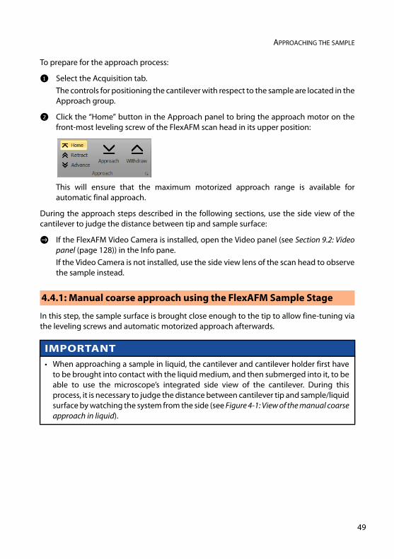
2 Click the “Home” button in the Approach panel to bring the approach motor on thefront-most leveling screw of the FlexAFM scan head in its upper position:
This will ensure that the maximum motorized approach range is available forautomatic final approach.
During the approach steps described in the following sections, use the side view of thecantilever to judge the distance between tip and sample surface:
> If the FlexAFM Video Camera is installed, open the Video panel (see Section 9.2: Videopanel (page 128)) in the Info pane. If the Video Camera is not installed, use the side view lens of the scan head to observethe sample instead.
In this step, the sample surface is brought close enough to the tip to allow fine-tuning viathe leveling screws and automatic motorized approach afterwards.
4.4.1: Manual coarse approach using the FlexAFM Sample Stage
IMPORTANT• When approaching a sample in liquid, the cantilever and cantilever holder first have
to be brought into contact with the liquid medium, and then submerged into it, to beable to use the microscope’s integrated side view of the cantilever. During thisprocess, it is necessary to judge the distance between cantilever tip and sample/liquidsurface by watching the system from the side (see Figure 4-1: View of the manual coarseapproach in liquid).
49
CHAPTER 4: A FIRST MEASUREMENT
5
To perform a manual coarse approach:
1 Use the leveling screws to bring the scan head in a position that is approximatelyparallel to the sample surface.
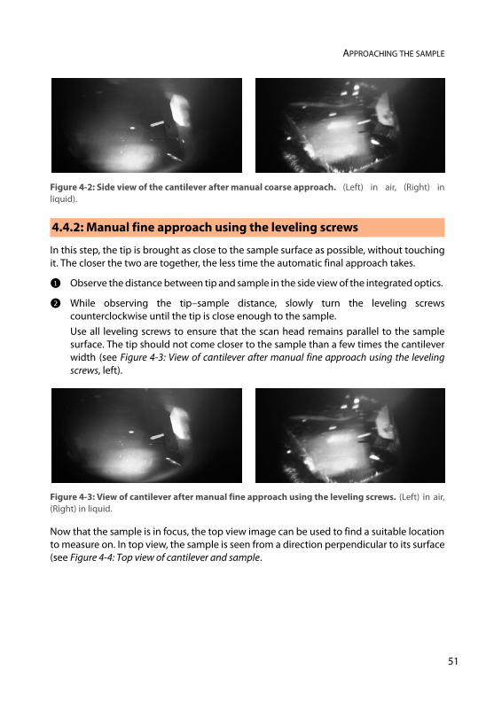
2 Slowly turn the manual Z-axis adjustment knob on the FlexAFM sample stageclockwise to bring the sample surface to within 1 mm of the cantilever tip.The side view should now look as shown in Figure 4-2: Side view of the cantilever aftermanual coarse approach. When the sample is reflective, the mirror image of thecantilever should be visible. When the sample is not reflective, the shadow of thecantilever may be visible. If neither a mirror image nor a shadow is visible, change theenvironment light until it is. You can use the cantilever as a ruler to judge distances inthe views of the integrated optics.
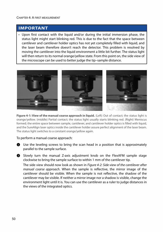
• Upon first contact with the liquid and/or during the initial immersion phase, thestatus light might start blinking red. This is due to the fact that the space betweencantilever and cantilever holder optics has not yet completely filled with liquid, andthe laser beam therefore doesn’t reach the detector. This problem is resolved bymoving the cantilever into the liquid environment a little bit further. The status lightwill then return to its normal orange/yellow state. From this point on, the side view ofthe microscope can be used to better judge the tip–sample distance.
Figure 4-1: View of the manual coarse approach in liquid. (Left) Out of contact; the status light isorange/yellow. (middle) Partial contact; the status light usually starts blinking red. (Right) Meniscusformed; the entire space between sample, cantilever, and cantilever holder optics is filled with liquid,and the SureAlign laser optics inside the cantilever holder assure perfect alignment of the laser beam.The status light switches to a constant orange/yellow again.
IMPORTANT
0
APPROACHING THE SAMPLE
In this step, the tip is brought as close to the sample surface as possible, without touchingit. The closer the two are together, the less time the automatic final approach takes.
1 Observe the distance between tip and sample in the side view of the integrated optics.
2 While observing the tip–sample distance, slowly turn the leveling screwscounterclockwise until the tip is close enough to the sample. Use all leveling screws to ensure that the scan head remains parallel to the samplesurface. The tip should not come closer to the sample than a few times the cantileverwidth (see Figure 4-3: View of cantilever after manual fine approach using the levelingscrews, left).
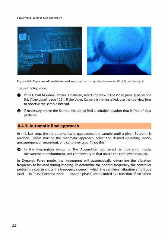
Now that the sample is in focus, the top view image can be used to find a suitable locationto measure on. In top view, the sample is seen from a direction perpendicular to its surface(see Figure 4-4: Top view of cantilever and sample.
Figure 4-2: Side view of the cantilever after manual coarse approach. (Left) in air, (Right) inliquid).
4.4.2: Manual fine approach using the leveling screws
Figure 4-3: View of cantilever after manual fine approach using the leveling screws. (Left) in air,(Right) in liquid.
51
CHAPTER 4: A FIRST MEASUREMENT
5
To use the top view:
1 If the FlexAFM Video Camera is installed, select Top view in the Video panel (see Section9.2: Video panel (page 128)). If the Video Camera is not installed, use the top view lensto observe the sample instead.
2 If necessary, move the Sample Holder to find a suitable location that is free of dustparticles.
In this last step, the tip automatically approaches the sample until a given Setpoint isreached. Before starting the automatic approach, select the desired operating mode,measurement environment, and cantilever type. To do this:
> In the Preparation group of the Acquisition tab, select an operating mode,measurement environment, and cantilever type that match the cantilever installed.
In Dynamic Force mode, the instrument will automatically determine the vibrationfrequency to be used during imaging. To determine the optimal frequency, the controllerperforms a coarse and a fine frequency sweep in which the cantilever vibration amplitude(and — in Phase Contrast mode — also the phase) are recorded as a function of excitation
Figure 4-4: Top view of cantilever and sample. (Left) chip structure in air, (Right) cells in liquid.
4.4.3: Automatic final approach
2
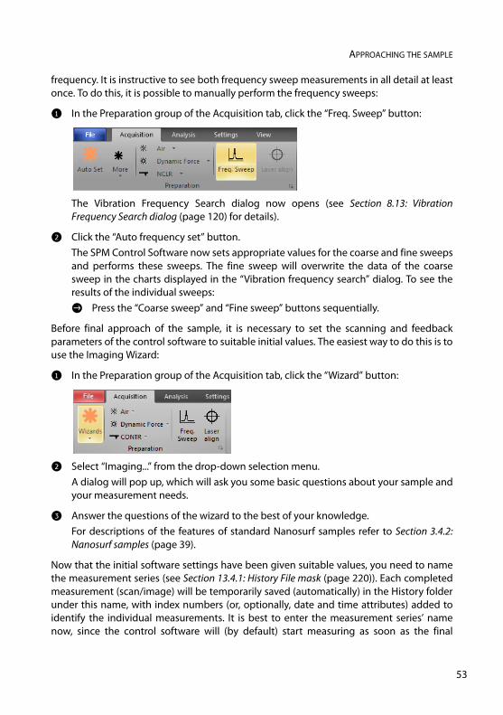
APPROACHING THE SAMPLE
frequency. It is instructive to see both frequency sweep measurements in all detail at leastonce. To do this, it is possible to manually perform the frequency sweeps:
1 In the Preparation group of the Acquisition tab, click the “Freq. Sweep” button:
The Vibration Frequency Search dialog now opens (see Section 8.13: VibrationFrequency Search dialog (page 120) for details).
2 Click the “Auto frequency set” button.The SPM Control Software now sets appropriate values for the coarse and fine sweepsand performs these sweeps. The fine sweep will overwrite the data of the coarsesweep in the charts displayed in the “Vibration frequency search” dialog. To see theresults of the individual sweeps:> Press the “Coarse sweep” and “Fine sweep” buttons sequentially.
Before final approach of the sample, it is necessary to set the scanning and feedbackparameters of the control software to suitable initial values. The easiest way to do this is touse the Imaging Wizard:
1 In the Preparation group of the Acquisition tab, click the “Wizard” button:
2 Select “Imaging...” from the drop-down selection menu.A dialog will pop up, which will ask you some basic questions about your sample andyour measurement needs.
3 Answer the questions of the wizard to the best of your knowledge.For descriptions of the features of standard Nanosurf samples refer to Section 3.4.2:Nanosurf samples (page 39).
Now that the initial software settings have been given suitable values, you need to namethe measurement series (see Section 13.4.1: History File mask (page 220)). Each completedmeasurement (scan/image) will be temporarily saved (automatically) in the History folderunder this name, with index numbers (or, optionally, date and time attributes) added toidentify the individual measurements. It is best to enter the measurement series’ namenow, since the control software will (by default) start measuring as soon as the final
53
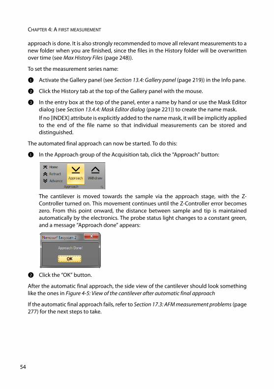
CHAPTER 4: A FIRST MEASUREMENT
5
approach is done. It is also strongly recommended to move all relevant measurements to anew folder when you are finished, since the files in the History folder will be overwrittenover time (see Max History Files (page 248)).
To set the measurement series name:
1 Activate the Gallery panel (see Section 13.4: Gallery panel (page 219)) in the Info pane.
2 Click the History tab at the top of the Gallery panel with the mouse.
3 In the entry box at the top of the panel, enter a name by hand or use the Mask Editordialog (see Section 13.4.4: Mask Editor dialog (page 221)) to create the name mask.If no [INDEX] attribute is explicitly added to the name mask, it will be implicitly appliedto the end of the file name so that individual measurements can be stored anddistinguished.
The automated final approach can now be started. To do this:
1 In the Approach group of the Acquisition tab, click the “Approach” button:
The cantilever is moved towards the sample via the approach stage, with the Z-Controller turned on. This movement continues until the Z-Controller error becomeszero. From this point onward, the distance between sample and tip is maintainedautomatically by the electronics. The probe status light changes to a constant green,and a message “Approach done” appears:
2 Click the “OK” button.
After the automatic final approach, the side view of the cantilever should look somethinglike the ones in Figure 4-5: View of the cantilever after automatic final approach
If the automatic final approach fails, refer to Section 17.3: AFM measurement problems (page277) for the next steps to take.
4
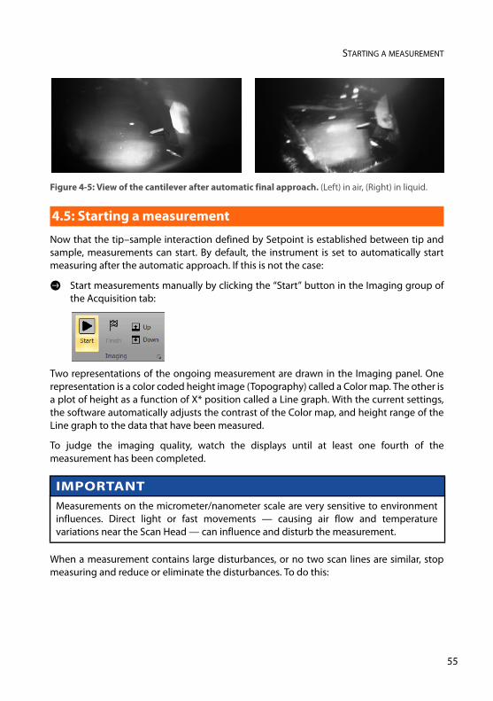
STARTING A MEASUREMENT
Now that the tip–sample interaction defined by Setpoint is established between tip andsample, measurements can start. By default, the instrument is set to automatically startmeasuring after the automatic approach. If this is not the case:
> Start measurements manually by clicking the “Start” button in the Imaging group ofthe Acquisition tab:
Two representations of the ongoing measurement are drawn in the Imaging panel. Onerepresentation is a color coded height image (Topography) called a Color map. The other isa plot of height as a function of X* position called a Line graph. With the current settings,the software automatically adjusts the contrast of the Color map, and height range of theLine graph to the data that have been measured.
To judge the imaging quality, watch the displays until at least one fourth of themeasurement has been completed.
When a measurement contains large disturbances, or no two scan lines are similar, stopmeasuring and reduce or eliminate the disturbances. To do this:
Figure 4-5: View of the cantilever after automatic final approach. (Left) in air, (Right) in liquid.
4.5: Starting a measurement
IMPORTANTMeasurements on the micrometer/nanometer scale are very sensitive to environmentinfluences. Direct light or fast movements — causing air flow and temperaturevariations near the Scan Head — can influence and disturb the measurement.
55
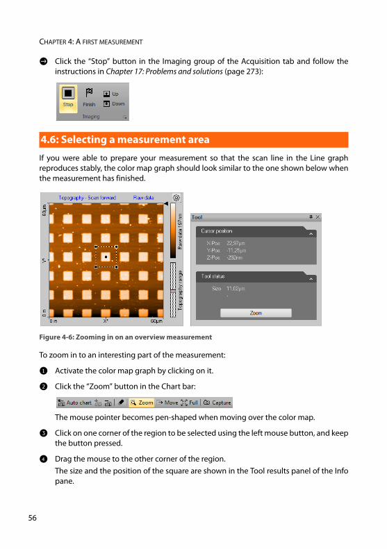
CHAPTER 4: A FIRST MEASUREMENT
5
> Click the “Stop” button in the Imaging group of the Acquisition tab and follow theinstructions in Chapter 17: Problems and solutions (page 273):
If you were able to prepare your measurement so that the scan line in the Line graphreproduces stably, the color map graph should look similar to the one shown below whenthe measurement has finished.
To zoom in to an interesting part of the measurement:
1 Activate the color map graph by clicking on it.
2 Click the “Zoom” button in the Chart bar:
The mouse pointer becomes pen-shaped when moving over the color map.
3 Click on one corner of the region to be selected using the left mouse button, and keepthe button pressed.
4 Drag the mouse to the other corner of the region.The size and the position of the square are shown in the Tool results panel of the Infopane.
4.6: Selecting a measurement area
Figure 4-6: Zooming in on an overview measurement
6
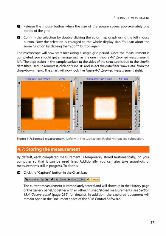
STORING THE MEASUREMENT
5 Release the mouse button when the size of the square covers approximately oneperiod of the grid.
6 Confirm the selection by double clicking the color map graph using the left mousebutton. Now the selection is enlarged to the whole display size. You can abort thezoom function by clicking the “Zoom” button again.
The microscope will now start measuring a single grid period. Once the measurement iscompleted, you should get an image such as the one in Figure 4-7: Zoomed measurement,left. The depression in the sample surface to the sides of the structure is due to the LineFitdata filter used. To remove it, click on “LineFit” and select the data filter “Raw Data” from thedrop-down menu. The chart will now look like Figure 4-7: Zoomed measurement, right.
By default, each completed measurement is temporarily stored (automatically) on yourcomputer so that it can be used later. Additionally, you can also take snapshots ofmeasurements still in progress. To do this:
> Click the “Capture” button in the Chart bar:
The current measurement is immediately stored and will show up in the History pageof the Gallery panel, together with all other finished/stored measurements (see Section13.4: Gallery panel (page 219) for details). In addition, the captured document willremain open in the Document space of the SPM Control Software.
Figure 4-7: Zoomed measurement. (Left) with line subtraction, (Right) without line subtraction.
4.7: Storing the measurement
57
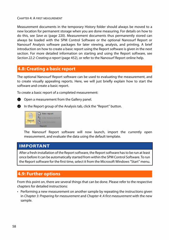
CHAPTER 4: A FIRST MEASUREMENT
5
Measurement documents in the temporary History folder should always be moved to anew location for permanent storage when you are done measuring. For details on how todo this, see Save as (page 220). Measurement documents thus permanently stored canalways be loaded with the SPM Control Software or the optional Nanosurf Report orNanosurf Analysis software packages for later viewing, analysis, and printing. A briefintroduction on how to create a basic report using the Report software is given in the nextsection. For more detailed information on starting and using the Report software, seeSection 22.2: Creating a report (page 452), or refer to the Nanosurf Report online help.
The optional Nanosurf Report software can be used to evaluating the measurement, andto create visually appealing reports. Here, we will just briefly explain how to start thesoftware and create a basic report.
To create a basic report of a completed measurement:
1 Open a measurement from the Gallery panel.
2 In the Report group of the Analysis tab, click the “Report” button.
The Nanosurf Report software will now launch, import the currently openmeasurement, and evaluate the data using the default template.
From this point on, there are several things that can be done. Please refer to the respectivechapters for detailed instructions:• Performing a new measurement on another sample by repeating the instructions given
in Chapter 3: Preparing for measurement and Chapter 4: A first measurement with the newsample.
4.8: Creating a basic report
IMPORTANTAfter a fresh installation of the Report software, the Report software has to be run at leastonce before it can be automatically started from within the SPM Control Software. To runthe Report software for the first time, select it from the Microsoft Windows “Start” menu.
4.9: Further options
8
FURTHER OPTIONS
• Performing a new measurement in a different measurement environment by adding/removing liquid to/from the sample and repeating the instructions given in Chapter 3:Introduction and Chapter 4: A first measurement for the new measurement environment.
• Improving measurement quality, as described in Chapter 5: Improving measurementquality (page 61).
• Performing a different type of measurement by choosing a different operating mode, asdescribed in Chapter 6: Operating modes (page 66).
• Finishing measurements, turning off the instrument, and/or storing the instrument, asdescribed in Chapter 6: Finishing measurements (page 69).
TipIf you want to measure a single sample in air as well as in liquid, always perform themeasurements in air first. This way, you will be able to judge sample height and performsample approach more easily, as the manual coarse approach is more easily performedin air. It is also better for the cantilever to change from air to liquid than the reverse. Acantilever that has been exposed to liquid will — even when properly dried — neverhave the exact same physical properties as a cantilever that has never been exposed toliquid before. Therefore, only use cantilevers that have been exposed to liquidenvironments for new measurements in liquid.
59

CHAPTER 4: A FIRST MEASUREMENT
6
0
CHAPTER 5:
Improving measurement quality0
0
CHAPTER 5: IMPROVING MEASUREMENT QUALITY
6
Interfering signals can be recognized because they have a fixed frequency, usually amultiple of the local mains frequency (50 or 60 Hz) throughout the image. Thus, they aremanifested by straight lines that run throughout the entire image.
Possible interference sources are:• Mechanical vibrations from machines or heavy transformers in direct vicinity (e.g.
pumps).• Electrical interference (in the electronics, or in electrical forces of the tip–sample
interaction).• Infrared and other light sources (light bulbs, sample illumination in an inverted
microscope).
Measure the frequency of the vibrations to find out if the interference is due to mechanicalvibrations. Such vibrations have a frequency that is (a multiple of ) the rotation frequencyof the source. This frequency is usually not a multiple of the local mains frequency, and maychange slightly over time. Try the following to find out if the interfering signal is due tomechanical vibrations:
1 If possible, turn off all rotating machines (i.e. pumps) in the room.
2 Change the vibration isolation by putting the Scan Head directly on the table, insteadof on the Sample stage.
To reduce the influence of these vibrations, either improve the isolation of these machines,or improve the isolation of the instrument by using an active vibration isolation table (e.g.the optional Nanosurf Isostage or halcyonics_i4.
Electrical interference may be caused by interference in the electronics, or by electrostaticforces acting between the tip and the sample. Try the following in order to reduce theinfluence of electrical interference:
1 Connect the instrument to the mains power supply using sockets with line filters andsurge protection.
2 Connect the sample, the sample support, the Sample Holder to the ground connectoron the Scan Head using the ground cable (Figure 1-2: Contents of the Tool set (page 18),item 1).
5.1: Removing interfering signals
5.1.1: Mechanical vibrations
5.1.2: Electrical interference
2
ADJUSTING THE MEASUREMENT PLANE
3 Remove interfering electromagnetic field sources, such cathode ray tube displays,loudspeakers, etc.
Infrared and other light sources can influence the cantilever deflection detection system.This problem is especially severe when measuring in the Static Force mode. Try thefollowing in order to reduce the influence of infrared light sources:
1 Turn off the light.
2 Shield the instrument from external light sources.
3 When using the instrument with an inverted microscope, use filters that filter outinfrared light.
Ideally, the sample surface and the XY-plane of the scanner run parallel to each other. Inmost cases, however, the sample plane is tilted with respect to the XY-plane of the scanner.In this case, the sample cross section in the X* measurement direction has a certain slope.The Line graph chart in Figure 5-1: Maladjusted slope is an example.
This slope depends on the direction of the X* direction and therefore on the rotation of themeasurement, as shown in Figure 5-2: Sample and measurement orientation before slopeadjustment.
This slope is undesirable for several reasons:• It makes it difficult to see small details on the sample surface, because the Average, Plane
fit, or higher order filters cannot be used properly.• The Z-Controller functions less accurately, because it continuously has to compensate for
the sample slope.
Ideally, the XY-plane of the scanner has already been correctly aligned with the sampleplane using the three leveling screws on the Scan Head. This alignment can, however, noteasily be performed once the automatic approach has been done, as this would damagethe tip. After approach, the measurement plane should therefore be adjustedelectronically. This can be done automatically or manually. Both procedures are describedbelow.
5.1.3: Infrared and other light sources
5.2: Adjusting the measurement plane
63
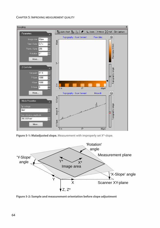
CHAPTER 5: IMPROVING MEASUREMENT QUALITY
6
Figure 5-1: Maladjusted slope. Measurement with improperly set X*-slope.
Figure 5-2: Sample and measurement orientation before slope adjustment
XY
Z, Z*
Scanner XY-plane
'X-Slope' angle
'Y-Slope' angle
'Rotation' angle
Measurement plane
Image areaX*Y*
4
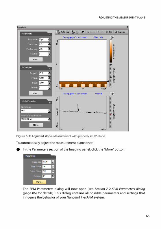
ADJUSTING THE MEASUREMENT PLANE
To automatically adjust the measurement plane once:
1 In the Parameters section of the Imaging panel, click the “More” button:
The SPM Parameters dialog will now open (see Section 7.9: SPM Parameters dialog(page 86) for details). This dialog contains all possible parameters and settings thatinfluence the behavior of your Nanosurf FlexAFM system.
Figure 5-3: Adjusted slope. Measurement with properly set X*-slope.
65
CHAPTER 5: IMPROVING MEASUREMENT QUALITY
6
2 Make sure that “Imaging” is selected in the SPM Parameters dialog:
3 Click the “Adjust slope” button:
The SPM Control Software will automatically perform a slope determinationprocedure similar to the manual procedure described below and will enter the slopeangles into the X- and Y-Slope parameters.
To automatically adjust the measurement plane before each measurement:
> Check the “Auto set” checkbox next to the “Adjust slope” button.
To manually adjust the measurement plane:
1 Measure the slope for X in the Line graph using the angle tool (see Measure Angle(page 227)). Use a single click instead of dragging the first line to create a horizontal line andmeasure the angle relative to the X*-Axis.
2 Enter the result of the angle determination as X-Slope (see Imaging options (page 160))and fine-tune its value until the X-axis of the scan line lies parallel to the X-axis of thesample.
3 Set Rotation to 90° to scan along the Y-direction of the scanner.
4 If the scan line in Y-direction is not horizontal, perform the same procedure asdescribed for correction of the slope in X but now for Y.
5 Reset “Rotation” to 0°. The scanner scans in X-direction again.
IMPORTANTIf the sample surface contains large jumps or steps in height, the line fitting procedureused to determine the slope in X- and Y-direction may not deliver the best possibleresults. In such cases it is recommended to perform a manual slope adjustment asdescribed below.
6
JUDGING TIP QUALITY
When all prerequisites for measurement are optimal, the measurement quality mainlydepends on the quality of the tip. A good tip quality is essential for high quality images andhigh resolution.
When the image quality deteriorates dramatically during a previously good measurement,the tip has most probably picked up some material from the sample. As a result, the imagein the color map charts consist of uncorrelated lines or the image appear blurred (seeChapter 5: Measurement containing tip artifacts). In such cases:
> Follow the suggestions in Section 17.3.3: Image quality suddenly deteriorates (page 279). If these do not help, the cantilever should be replaced.
When all peaks in the image have the same, usually triangular shape, the sharp end of thetip may have broken off. The measured structure reflects the shape of the tip rather thanthat of the sample and is called a tip artefact. In such cases:
> Replace the cantilever.
5.3: Judging tip quality
Figure 5-4: Measurement containing tip artifacts
67

CHAPTER 5: IMPROVING MEASUREMENT QUALITY
6
8
CHAPTER 6:
Finishing measurements0
0
CHAPTER 6: FINISHING MEASUREMENTS
7
Once you are done measuring:
1 In the Imaging group of the Acquisition tab, click the “Stop” button to stop measuring.
2 Open the positioning window.
3 If the FlexAFM Video Camera is installed, activate “Side view” in the Video panel (seeSection 9.2: Video panel (page 128)). If the Video Camera is not installed, use the side view lens of the scan head to observethe sample instead.
4 Retract the cantilever to a safe distance from the sample by clicking and holding the“Retract” button in the Approach group of the Acquisition tab until the tip–sampledistance is at least as large as shown in Figure 6-1: Side view of the cantilever afterretracting or by clicking the “Home” button and waiting for the automatic fullwithdrawal process to finish.
5 Turn down the sample platform of the FlexAFM sample stage.
6 Remove the sample or sample holder from the sample stage.
7 In case the measurement was performed in liquid, remove and clean sample holder,cantilever, and sample as described in Section 3.3.2: Removing the Cantilever Holder(page 35) and follow the instructions describing the removal of a used cantilever inSection 3.3.3: Inserting the cantilever in the Cantilever Holder (page 36).
To turn off the instrument:
1 Finish as described in Section 6.1: Finishing scanning
6.1: Finishing scanning
Figure 6-1: Side view of the cantilever after retracting. Minimal distance required for safe removalof the scan head and sample. (Left) in air, (Right) in liquid.
6.2: Turning off the instrument
0
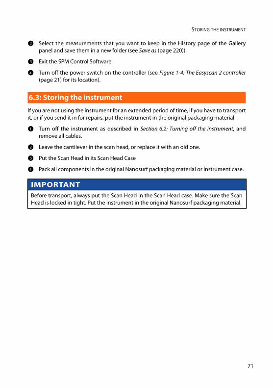
STORING THE INSTRUMENT
2 Select the measurements that you want to keep in the History page of the Gallerypanel and save them in a new folder (see Save as (page 220)).
3 Exit the SPM Control Software.
4 Turn off the power switch on the controller (see Figure 1-4: The Easyscan 2 controller(page 21) for its location).
If you are not using the instrument for an extended period of time, if you have to transportit, or if you send it in for repairs, put the instrument in the original packaging material.
1 Turn off the instrument as described in Section 6.2: Turning off the instrument, andremove all cables.
2 Leave the cantilever in the scan head, or replace it with an old one.
3 Put the Scan Head in its Scan Head Case
4 Pack all components in the original Nanosurf packaging material or instrument case.
6.3: Storing the instrument
IMPORTANTBefore transport, always put the Scan Head in the Scan Head case. Make sure the ScanHead is locked in tight. Put the instrument in the original Nanosurf packaging material.
71

CHAPTER 6: FINISHING MEASUREMENTS
7
2
PART B:
SOFTWARE REFERENCE


CHAPTER 7:
The user interface0
0
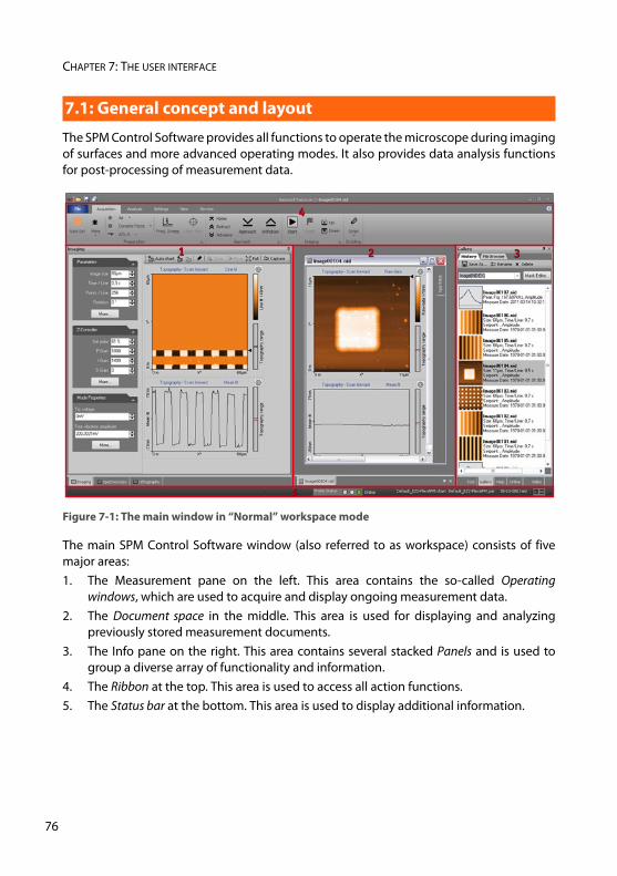
CHAPTER 7: THE USER INTERFACE
7
The SPM Control Software provides all functions to operate the microscope during imagingof surfaces and more advanced operating modes. It also provides data analysis functionsfor post-processing of measurement data.
The main SPM Control Software window (also referred to as workspace) consists of fivemajor areas:1. The Measurement pane on the left. This area contains the so-called Operating
windows, which are used to acquire and display ongoing measurement data.2. The Document space in the middle. This area is used for displaying and analyzing
previously stored measurement documents.3. The Info pane on the right. This area contains several stacked Panels and is used to
group a diverse array of functionality and information.4. The Ribbon at the top. This area is used to access all action functions.5. The Status bar at the bottom. This area is used to display additional information.
7.1: General concept and layout
Figure 7-1: The main window in “Normal” workspace mode
11 22 33
44
55
6
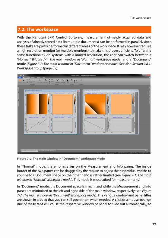
THE WORKSPACE
With the Nanosurf SPM Control Software, measurement of newly acquired data andanalysis of already stored data (in multiple documents) can be performed in parallel, sincethese tasks are partly performed in different areas of the workspace. It may however requirea high resolution monitor (or multiple monitors) to make this process efficient. To offer thesame functionality on systems with a limited resolution, the user can switch between a“Normal” (Figure 7-1: The main window in “Normal” workspace mode) and a “Document”mode (Figure 7-2: The main window in “Document” workspace mode). See also Section 7.8.1:Workspace group (page 85).
In “Normal” mode, the emphasis lies on the Measurement and Info panes. The insideborder of the two panes can be dragged by the mouse to adjust their individual widths toyour needs. Document space on the other hand is rather limited (see Figure 7-1: The mainwindow in “Normal” workspace mode). This mode is most suited for measurements.
In “Document” mode, the Document space is maximized while the Measurement and Infopanes are minimized to the left and right side of the main window, respectively (see Figure7-2: The main window in “Document” workspace mode). The various window and panel titlesare shown in tabs so that you can still open them when needed. A click or a mouse-over onone of these tabs will cause the respective window or panel to slide out automatically, so
7.2: The workspace
Figure 7-2: The main window in “Document” workspace mode
77
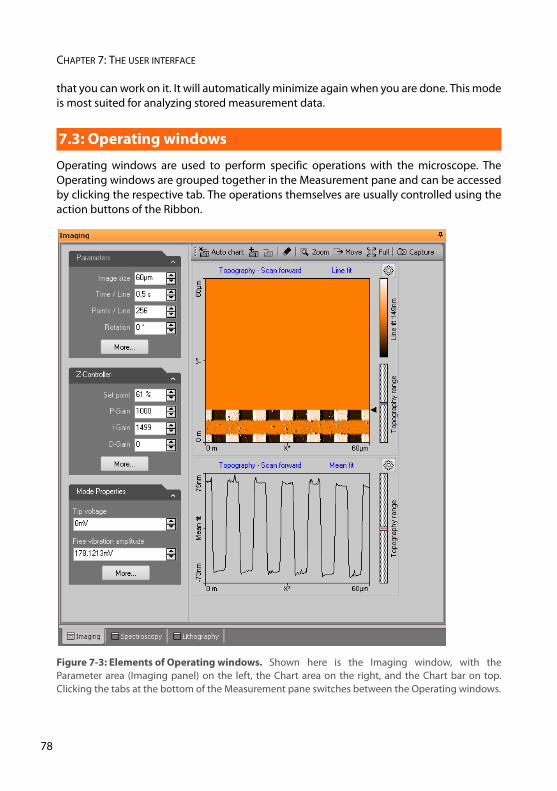
CHAPTER 7: THE USER INTERFACE
7
that you can work on it. It will automatically minimize again when you are done. This modeis most suited for analyzing stored measurement data.
Operating windows are used to perform specific operations with the microscope. TheOperating windows are grouped together in the Measurement pane and can be accessedby clicking the respective tab. The operations themselves are usually controlled using theaction buttons of the Ribbon.
7.3: Operating windows
Figure 7-3: Elements of Operating windows. Shown here is the Imaging window, with theParameter area (Imaging panel) on the left, the Chart area on the right, and the Chart bar on top.Clicking the tabs at the bottom of the Measurement pane switches between the Operating windows.
8
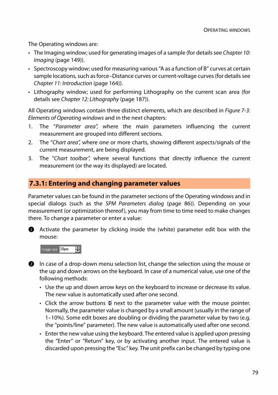
OPERATING WINDOWS
The Operating windows are:• The Imaging window; used for generating images of a sample (for details see Chapter 10:
Imaging (page 149)).• Spectroscopy window; used for measuring various “A as a function of B” curves at certain
sample locations, such as force–Distance curves or current-voltage curves (for details seeChapter 11: Introduction (page 164)).
• Lithography window; used for performing Lithography on the current scan area (fordetails see Chapter 12: Lithography (page 187)).
All Operating windows contain three distinct elements, which are described in Figure 7-3:Elements of Operating windows and in the next chapters:1. The “Parameter area”, where the main parameters influencing the current
measurement are grouped into different sections.2. The “Chart area”, where one or more charts, showing different aspects/signals of the
current measurement, are being displayed.3. The “Chart toolbar”, where several functions that directly influence the current
measurement (or the way its displayed) are located.
Parameter values can be found in the parameter sections of the Operating windows and inspecial dialogs (such as the SPM Parameters dialog (page 86)). Depending on yourmeasurement (or optimization thereof), you may from time to time need to make changesthere. To change a parameter or enter a value:
1 Activate the parameter by clicking inside the (white) parameter edit box with themouse:
2 In case of a drop-down menu selection list, change the selection using the mouse orthe up and down arrows on the keyboard. In case of a numerical value, use one of thefollowing methods:• Use the up and down arrow keys on the keyboard to increase or decrease its value.
The new value is automatically used after one second.• Click the arrow buttons next to the parameter value with the mouse pointer.
Normally, the parameter value is changed by a small amount (usually in the range of1–10%). Some edit boxes are doubling or dividing the parameter value by two (e.g.the “points/line” parameter). The new value is automatically used after one second.
• Enter the new value using the keyboard. The entered value is applied upon pressingthe “Enter” or “Return” key, or by activating another input. The entered value isdiscarded upon pressing the “Esc” key. The unit prefix can be changed by typing one
7.3.1: Entering and changing parameter values
79
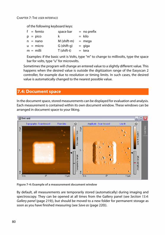
CHAPTER 7: THE USER INTERFACE
8
of the following keyboard keys:
Examples: if the basic unit is Volts, type “m” to change to millivolts, type the spacebar for volts, type “u” for microvolts.
Sometimes the program will change an entered value to a slightly different value. Thishappens when the desired value is outside the digitization range of the Easyscan 2controller, for example due to resolution or timing limits. In such cases, the desiredvalue is automatically changed to the nearest possible value.
In the document space, stored measurements can be displayed for evaluation and analysis.Each measurement is contained within its own document window. These windows can bearranged in document space to your liking.
By default, all measurements are temporarily stored (automatically) during imaging andspectroscopy. They can be opened at all times from the Gallery panel (see Section 13.4:Gallery panel (page 219)), but should be moved to a new folder for permanent storage assoon as you have finished measuring (see Save as (page 220)).
f = femto space bar = no prefixp = pico k = kilon = nano M (shift-m) = megau = micro G (shift-g) = gigam = milli T (shift-t) = tera
7.4: Document space
Figure 7-4: Example of a measurement document window
0
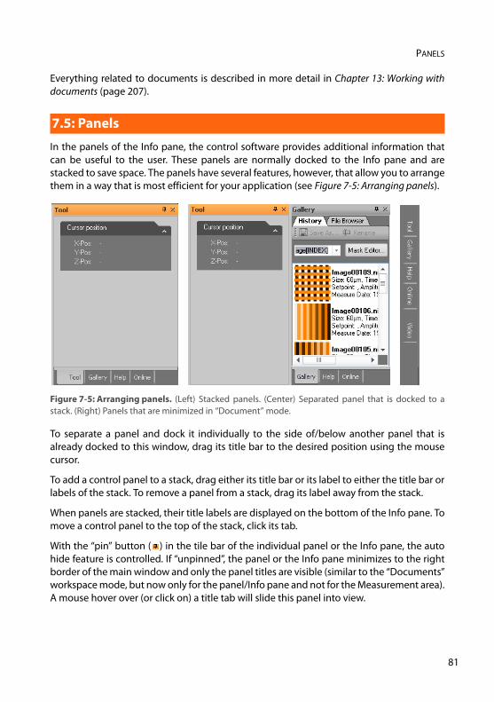
PANELS
Everything related to documents is described in more detail in Chapter 13: Working withdocuments (page 207).
In the panels of the Info pane, the control software provides additional information thatcan be useful to the user. These panels are normally docked to the Info pane and arestacked to save space. The panels have several features, however, that allow you to arrangethem in a way that is most efficient for your application (see Figure 7-5: Arranging panels).
To separate a panel and dock it individually to the side of/below another panel that isalready docked to this window, drag its title bar to the desired position using the mousecursor.
To add a control panel to a stack, drag either its title bar or its label to either the title bar orlabels of the stack. To remove a panel from a stack, drag its label away from the stack.
When panels are stacked, their title labels are displayed on the bottom of the Info pane. Tomove a control panel to the top of the stack, click its tab.
With the “pin” button ( ) in the tile bar of the individual panel or the Info pane, the autohide feature is controlled. If “unpinned”, the panel or the Info pane minimizes to the rightborder of the main window and only the panel titles are visible (similar to the “Documents”workspace mode, but now only for the panel/Info pane and not for the Measurement area).A mouse hover over (or click on) a title tab will slide this panel into view.
7.5: Panels
Figure 7-5: Arranging panels. (Left) Stacked panels. (Center) Separated panel that is docked to astack. (Right) Panels that are minimized in “Document” mode.
81
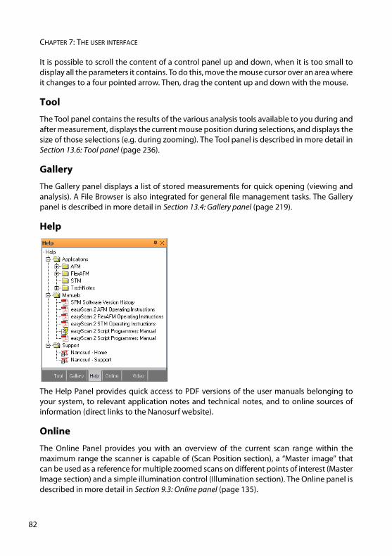
CHAPTER 7: THE USER INTERFACE
8
It is possible to scroll the content of a control panel up and down, when it is too small todisplay all the parameters it contains. To do this, move the mouse cursor over an area whereit changes to a four pointed arrow. Then, drag the content up and down with the mouse.
Tool
The Tool panel contains the results of the various analysis tools available to you during andafter measurement, displays the current mouse position during selections, and displays thesize of those selections (e.g. during zooming). The Tool panel is described in more detail inSection 13.6: Tool panel (page 236).
Gallery
The Gallery panel displays a list of stored measurements for quick opening (viewing andanalysis). A File Browser is also integrated for general file management tasks. The Gallerypanel is described in more detail in Section 13.4: Gallery panel (page 219).
Help
The Help Panel provides quick access to PDF versions of the user manuals belonging toyour system, to relevant application notes and technical notes, and to online sources ofinformation (direct links to the Nanosurf website).
Online
The Online Panel provides you with an overview of the current scan range within themaximum range the scanner is capable of (Scan Position section), a “Master image” thatcan be used as a reference for multiple zoomed scans on different points of interest (MasterImage section) and a simple illumination control (Illumination section). The Online panel isdescribed in more detail in Section 9.3: Online panel (page 135).
2
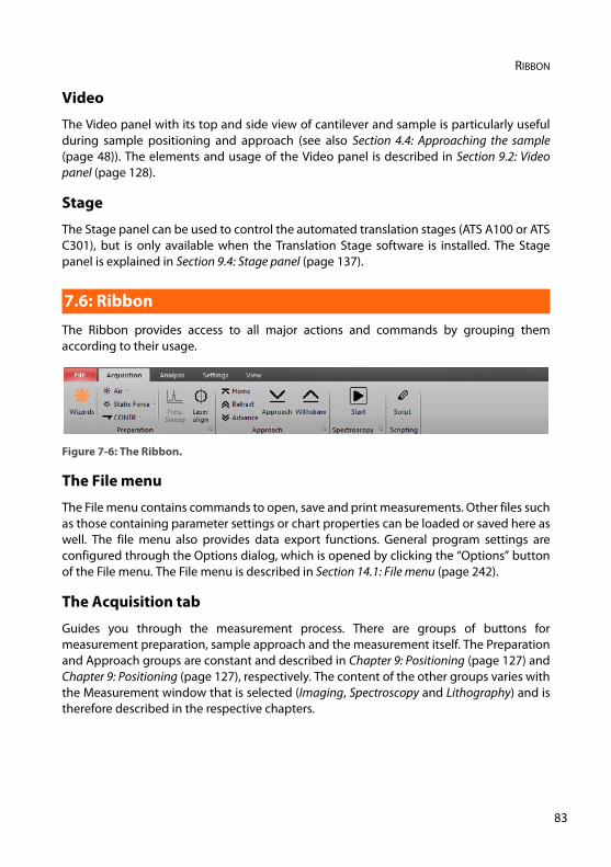
RIBBON
Video
The Video panel with its top and side view of cantilever and sample is particularly usefulduring sample positioning and approach (see also Section 4.4: Approaching the sample(page 48)). The elements and usage of the Video panel is described in Section 9.2: Videopanel (page 128).
Stage
The Stage panel can be used to control the automated translation stages (ATS A100 or ATSC301), but is only available when the Translation Stage software is installed. The Stagepanel is explained in Section 9.4: Stage panel (page 137).
The Ribbon provides access to all major actions and commands by grouping themaccording to their usage.
The File menu
The File menu contains commands to open, save and print measurements. Other files suchas those containing parameter settings or chart properties can be loaded or saved here aswell. The file menu also provides data export functions. General program settings areconfigured through the Options dialog, which is opened by clicking the “Options” buttonof the File menu. The File menu is described in Section 14.1: File menu (page 242).
The Acquisition tab
Guides you through the measurement process. There are groups of buttons formeasurement preparation, sample approach and the measurement itself. The Preparationand Approach groups are constant and described in Chapter 9: Positioning (page 127) andChapter 9: Positioning (page 127), respectively. The content of the other groups varies withthe Measurement window that is selected (Imaging, Spectroscopy and Lithography) and istherefore described in the respective chapters.
7.6: Ribbon
Figure 7-6: The Ribbon.
83
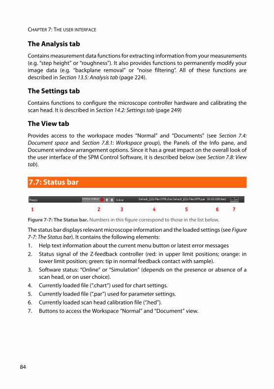
CHAPTER 7: THE USER INTERFACE
8
The Analysis tab
Contains measurement data functions for extracting information from your measurements(e.g. “step height” or “roughness”). It also provides functions to permanently modify yourimage data (e.g. “backplane removal” or “noise filtering”. All of these functions aredescribed in Section 13.5: Analysis tab (page 224).
The Settings tab
Contains functions to configure the microscope controller hardware and calibrating thescan head. It is described in Section 14.2: Settings tab (page 249)
The View tab
Provides access to the workspace modes “Normal” and “Documents” (see Section 7.4:Document space and Section 7.8.1: Workspace group), the Panels of the Info pane, andDocument window arrangement options. Since it has a great impact on the overall look ofthe user interface of the SPM Control Software, it is described below (see Section 7.8: Viewtab).
The status bar displays relevant microscope information and the loaded settings (see Figure7-7: The Status bar). It contains the following elements:1. Help text information about the current menu button or latest error messages2. Status signal of the Z-feedback controller (red: in upper limit positions; orange: in
lower limit position; green: tip in normal feedback contact with sample). 3. Software status: “Online” or “Simulation” (depends on the presence or absence of a
scan head, or on user choice).4. Currently loaded file (“.chart”) used for chart settings.5. Currently loaded file (“.par”) used for parameter settings.6. Currently loaded scan head calibration file (“.hed”).7. Buttons to access the Workspace “Normal” and “Document” view.
7.7: Status bar
1 2 3 4 5 6 7
Figure 7-7: The Status bar. Numbers in this figure correspond to those in the list below.
4
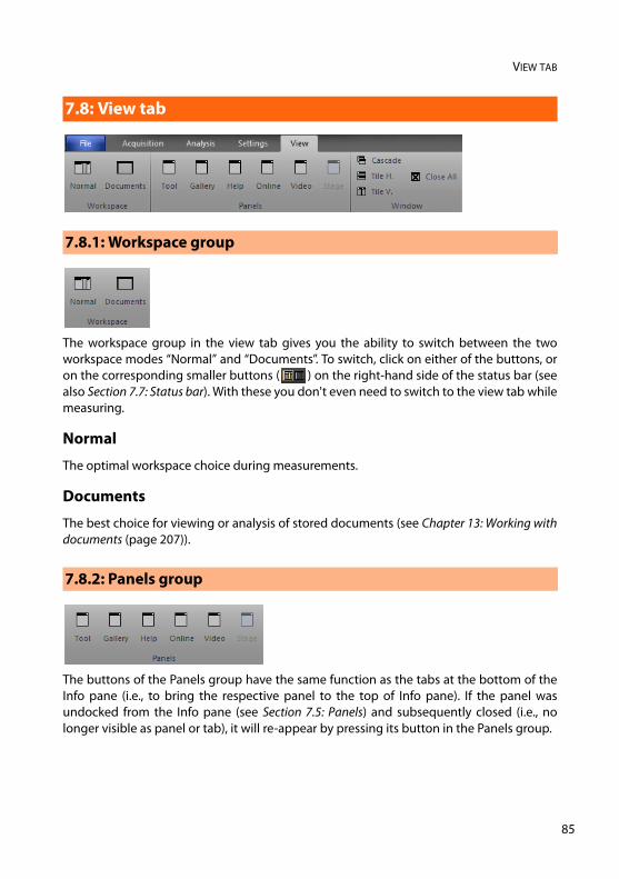
VIEW TAB
The workspace group in the view tab gives you the ability to switch between the twoworkspace modes “Normal” and “Documents”. To switch, click on either of the buttons, oron the corresponding smaller buttons ( ) on the right-hand side of the status bar (seealso Section 7.7: Status bar). With these you don't even need to switch to the view tab whilemeasuring.
Normal
The optimal workspace choice during measurements.
Documents
The best choice for viewing or analysis of stored documents (see Chapter 13: Working withdocuments (page 207)).
The buttons of the Panels group have the same function as the tabs at the bottom of theInfo pane (i.e., to bring the respective panel to the top of Info pane). If the panel wasundocked from the Info pane (see Section 7.5: Panels) and subsequently closed (i.e., nolonger visible as panel or tab), it will re-appear by pressing its button in the Panels group.
7.8: View tab
7.8.1: Workspace group
7.8.2: Panels group
85
CHAPTER 7: THE USER INTERFACE
8
The window group provides you with tools to arrange open measurement documents indifferent ways or quickly close them all.
Cascade
Open document windows are stacked on top of each other and slightly offset with respectto each other so that individual windows can be easily accessed. Width and position of thewindows is optimized by the control software.
Tile H.
Tiles the open document windows horizontally, so that individual measurements can beeasily compared. Width of the document windows is maximized. Height is evenlydistributed over the available document space.
Tile V.
Tiles the open document windows vertically, so that individual measurements can be easilycompared. Height of the document windows is maximized. Width is evenly distributedover the available document space.
Close all
Closes all open document windows. If unsaved data exists, you will be asked to save it.
While not directly visible upon starting the Nanosurf SPM Control software, the SPMParameters dialog is essential for controlling many advanced parameters duringmeasuring. The dialog is opened by clicking the “More” button that can be found in manyof the parameter sections of the measurement panels. It can stay open during all
IMPORTANTThe “Video” and “Stage” buttons are only available when the appropriate hardware ispresent.
7.8.3: Window group
7.9: SPM Parameters dialog
6
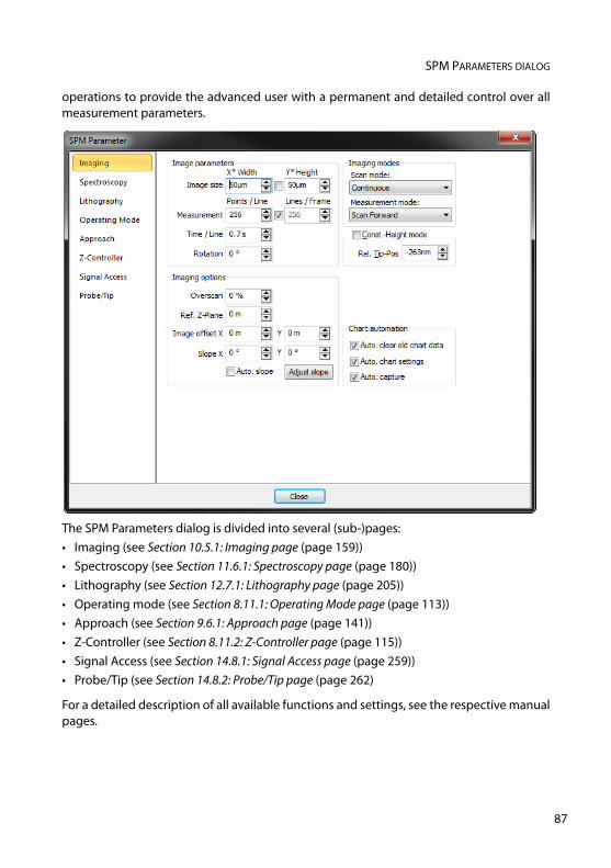
SPM PARAMETERS DIALOG
operations to provide the advanced user with a permanent and detailed control over allmeasurement parameters.
The SPM Parameters dialog is divided into several (sub-)pages:• Imaging (see Section 10.5.1: Imaging page (page 159))• Spectroscopy (see Section 11.6.1: Spectroscopy page (page 180))• Lithography (see Section 12.7.1: Lithography page (page 205))• Operating mode (see Section 8.11.1: Operating Mode page (page 113))• Approach (see Section 9.6.1: Approach page (page 141))• Z-Controller (see Section 8.11.2: Z-Controller page (page 115))• Signal Access (see Section 14.8.1: Signal Access page (page 259))• Probe/Tip (see Section 14.8.2: Probe/Tip page (page 262)
For a detailed description of all available functions and settings, see the respective manualpages.
87

CHAPTER 7: THE USER INTERFACE
8
8
CHAPTER 8:
Operating modes
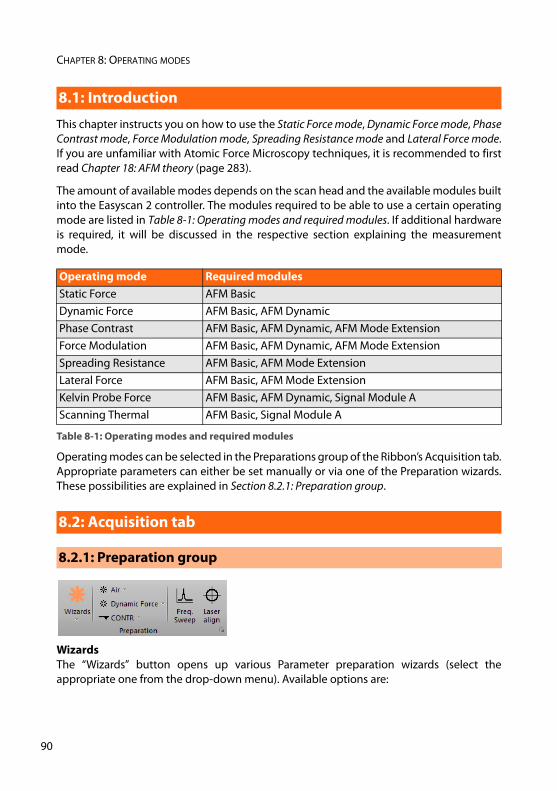
CHAPTER 8: OPERATING MODES
9
This chapter instructs you on how to use the Static Force mode, Dynamic Force mode, PhaseContrast mode, Force Modulation mode, Spreading Resistance mode and Lateral Force mode.If you are unfamiliar with Atomic Force Microscopy techniques, it is recommended to firstread Chapter 18: AFM theory (page 283).
The amount of available modes depends on the scan head and the available modules builtinto the Easyscan 2 controller. The modules required to be able to use a certain operatingmode are listed in Table 8-1: Operating modes and required modules. If additional hardwareis required, it will be discussed in the respective section explaining the measurementmode.
Operating modes can be selected in the Preparations group of the Ribbon’s Acquisition tab.Appropriate parameters can either be set manually or via one of the Preparation wizards.These possibilities are explained in Section 8.2.1: Preparation group.
WizardsThe “Wizards” button opens up various Parameter preparation wizards (select theappropriate one from the drop-down menu). Available options are:
8.1: Introduction
Operating mode Required modulesStatic Force AFM BasicDynamic Force AFM Basic, AFM DynamicPhase Contrast AFM Basic, AFM Dynamic, AFM Mode ExtensionForce Modulation AFM Basic, AFM Dynamic, AFM Mode ExtensionSpreading Resistance AFM Basic, AFM Mode ExtensionLateral Force AFM Basic, AFM Mode ExtensionKelvin Probe Force AFM Basic, AFM Dynamic, Signal Module AScanning Thermal AFM Basic, Signal Module A
Table 8-1: Operating modes and required modules
8.2: Acquisition tab
8.2.1: Preparation group
0
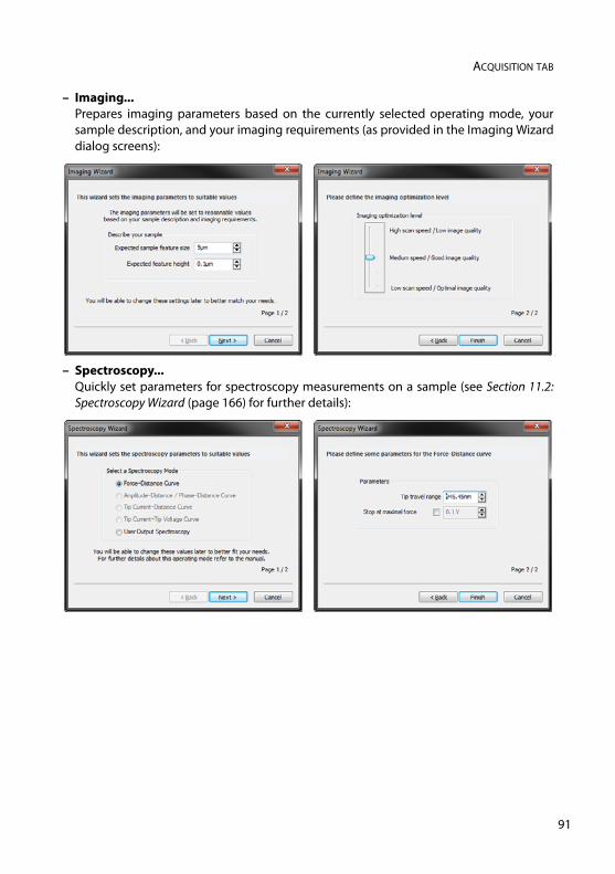
ACQUISITION TAB
– Imaging...Prepares imaging parameters based on the currently selected operating mode, yoursample description, and your imaging requirements (as provided in the Imaging Wizarddialog screens):
– Spectroscopy...Quickly set parameters for spectroscopy measurements on a sample (see Section 11.2:Spectroscopy Wizard (page 166) for further details):
91
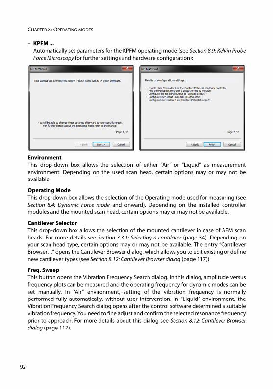
CHAPTER 8: OPERATING MODES
9
– KPFM ...Automatically set parameters for the KPFM operating mode (see Section 8.9: Kelvin ProbeForce Microscopy for further settings and hardware configuration):
Environment This drop-down box allows the selection of either “Air” or “Liquid” as measurementenvironment. Depending on the used scan head, certain options may or may not beavailable.
Operating Mode This drop-down box allows the selection of the Operating mode used for measuring (seeSection 8.4: Dynamic Force mode and onward). Depending on the installed controllermodules and the mounted scan head, certain options may or may not be available.
Cantilever SelectorThis drop-down box allows the selection of the mounted cantilever in case of AFM scanheads. For more details see Section 3.3.1: Selecting a cantilever (page 34). Depending onyour scan head type, certain options may or may not be available. The entry “CantileverBrowser…” opens the Cantilever Browser dialog, which allows you to edit existing or definenew cantilever types (see Section 8.12: Cantilever Browser dialog (page 117))
Freq. SweepThis button opens the Vibration Frequency Search dialog. In this dialog, amplitude versusfrequency plots can be measured and the operating frequency for dynamic modes can beset manually. In “Air” environment, setting of the vibration frequency is normallyperformed fully automatically, without user intervention. In “Liquid” environment, theVibration Frequency Search dialog opens after the control software determined a suitablevibration frequency. You need to fine adjust and confirm the selected resonance frequencyprior to approach. For more details about this dialog see Section 8.12: Cantilever Browserdialog (page 117).
2
STATIC FORCE MODE
Laser AlignThis button opens the Laser Align dialog. In this dialog, laser power and the currentposition of the laser beam on the detector are monitored. It is used to check for gooddetector and laser alignment. With FlexAFM scan heads it guides the user to manuallyadjust these positions if required or desired (see FlexAFM Laser and detector alignment).
Launcher iconMore advanced settings are available through the “Dialog Launcher” icon ( at the bottomright corner of the Preparation group), which opens up the SPM Parameters dialog on theOperating Mode page (see Section 8.11.1: Operating Mode page (page 113)).
In the Static Force mode, the “static” deflection of the cantilever is used as the error signalfor the Z-Controller. The Setpoint in Newton is calculated by multiplying the deflection withthe spring constant of the selected cantilever. In order to minimize tip/sample wear, theforce Setpoint should be made as small as possible. In some cases, even a negative Setpoint(i.e. an adhesive force) may work, but when the tip momentarily loses contact with thesample due to some disturbance, the Z-Controller will always fully retract the cantileverfrom the sample. Moreover, working in this range may cause image artifacts due toinstabilities in the tip–sample contact.
Both the Force Modulation mode and the Spreading Resistance mode are an extension ofthe Static Force mode.
The procedure for a first Static Force mode measurement is almost identical to theprocedure described for the Dynamic Force mode in Chapter 4: A first measurement (page45). In contrast to the description given there, however, do the following:
1 Select a cantilever suitable for static force mode (e.g. CONTR).
2 Install the cantilever as described in Section 3.3: Installing the cantilever (page 33).
3 Select this cantilever type in the Preparation group of the Acquisition tab.
4 Select the Static Force mode in this group as well.
5 Set the force Setpoint in the Z-Controller section of the Imaging window.
For a more detailed description of the parameters that can be set, refer to Section 8.11.1:Operating Mode page (page 113).
In the Dynamic Force mode, changes in the dynamic behavior of the cantilever aredetected by measuring changes in its vibration amplitude when it is excited with a
8.3: Static Force mode
8.4: Dynamic Force mode
93
CHAPTER 8: OPERATING MODES
9
sinusoidal signal with a frequency close to the free resonance frequency of the cantilever.When the cantilever tip comes close to the sample surface, this vibration amplitude willgenerally go down. Thus the Setpoint is the percentage of the vibration amplitude thatremains when the cantilever is close to the sample surface compared to the vibrationamplitude when the cantilever is far away from the surface. A small percentage means a bigreduction, and a large percentage means a small reduction. To minimize tip/sample wear,the Setpoint should be set as large as possible. However, when the Set-point becomes toolarge, the Z-Controller may not be able to optimally follow the sample surface, and artifactsmay occur due to instabilities in the cantilever vibration.
The procedure for a first Dynamic Force mode measurement is described for the DynamicForce mode in Chapter 4: A first measurement (page 45). For more information on how thevibration amplitude and frequency are set, refer to Section 8.11.1: Operating Mode page andSection 8.13: Vibration Frequency Search dialog.
The Phase Contrast mode is an extension of the Dynamic Force mode. Therefore, the samecantilevers can be used as for Dynamic force mode. In addition to the vibration amplitude,the phase shift between the cantilever vibration and a reference signal is measured. Thisphase shift changes when the resonance characteristic of the cantilever changes due tochanges in the tip–sample interaction. Thus, the Phase contrast mode can be used toproduce material contrast when there is a significant difference in the tip sampleinteraction of these materials. This section gives a brief description of how to operate theFlexAFM in phase contrast mode. For a more detailed description of the parameters thatcan be, refer to section Section 8.11.1: Operating Mode page (page 113).
The phase contrast mode can also be used to do Magnetic and Electrostatic ForceMicroscopy. For more information on how to do Magnetic Force Microscopy, refer totechnical note TN00031 Magnetic Force Microscopy, which can be downloaded from thesupport section of the Nanosurf web site at www.nanosurf.com.
Phase measurement
In Phase contrast mode, the phase of the measured cantilever vibration is compared to thephase of a reference sine wave. The phase comparison is performed by multiplying themeasured vibration signal with the reference. The measured phase, φmeasured , is the outputof this multiplication, and is related to the actual phase shift between the measuredvibration and the excitation sine wave, φactual , according to the following equation:
φmeasured = 90° sin ( φactual – φreference ) ,
where φreference is a reference phase that can be set by the user. This has two importantconsequences:
8.5: Phase Contrast mode
4
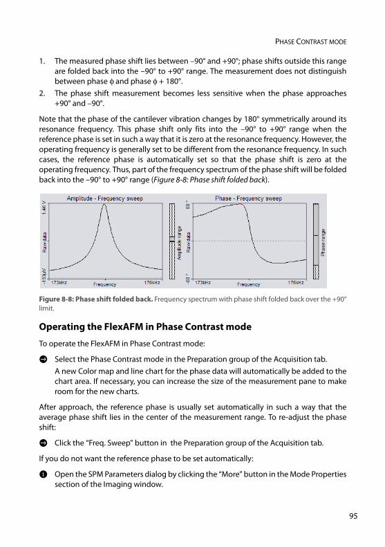
PHASE CONTRAST MODE
1. The measured phase shift lies between –90° and +90°; phase shifts outside this rangeare folded back into the –90° to +90° range. The measurement does not distinguishbetween phase φ and phase φ + 180°.
2. The phase shift measurement becomes less sensitive when the phase approaches+90° and –90°.
Note that the phase of the cantilever vibration changes by 180° symmetrically around itsresonance frequency. This phase shift only fits into the –90° to +90° range when thereference phase is set in such a way that it is zero at the resonance frequency. However, theoperating frequency is generally set to be different from the resonance frequency. In suchcases, the reference phase is automatically set so that the phase shift is zero at theoperating frequency. Thus, part of the frequency spectrum of the phase shift will be foldedback into the –90° to +90° range (Figure 8-8: Phase shift folded back).
Operating the FlexAFM in Phase Contrast mode
To operate the FlexAFM in Phase Contrast mode:
> Select the Phase Contrast mode in the Preparation group of the Acquisition tab.A new Color map and line chart for the phase data will automatically be added to thechart area. If necessary, you can increase the size of the measurement pane to makeroom for the new charts.
After approach, the reference phase is usually set automatically in such a way that theaverage phase shift lies in the center of the measurement range. To re-adjust the phaseshift:
> Click the “Freq. Sweep” button in the Preparation group of the Acquisition tab.
If you do not want the reference phase to be set automatically:
1 Open the SPM Parameters dialog by clicking the “More” button in the Mode Propertiessection of the Imaging window.
Figure 8-8: Phase shift folded back. Frequency spectrum with phase shift folded back over the +90°limit.
95
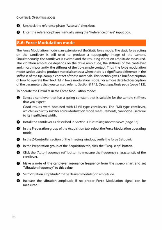
CHAPTER 8: OPERATING MODES
9
2 Uncheck the reference phase “Auto set” checkbox.
3 Enter the reference phase manually using the “Reference phase” input box.
The Force Modulation mode is an extension of the Static force mode. The static force actingon the cantilever is still used to produce a topography image of the sample.Simultaneously, the cantilever is excited and the resulting vibration amplitude measured.The vibration amplitude depends on the drive amplitude, the stiffness of the cantileverand, most importantly, the stiffness of the tip–sample contact. Thus, the force modulationmode can be used to produce material contrast when there is a significant difference in thestiffness of the tip–sample contact of these materials. This section gives a brief descriptionof how to operate the FlexAFM in force modulation mode. For a more detailed descriptionof the parameters that you can set, refer to Section 8.11.1: Operating Mode page (page 113).
To operate the FlexAFM in the Force Modulation mode:
1 Select a cantilever that has a spring constant that is suitable for the sample stiffnessthat you expect.Good results were obtained with LFMR-type cantilevers. The FMR type cantilever,which is explicitly sold for Force Modulation mode measurements, cannot be used dueto its insufficient width.
2 Install the cantilever as described in Section 3.3: Installing the cantilever (page 33).
3 In the Preparation group of the Acquisition tab, select the Force Modulation operatingmode.
4 In the Z-Controller section of the Imaging window, verify the force Setpoint.
5 In the Preparation group of the Acquisition tab, click the “Freq. seep” button.
6 Click the “Auto frequency set” button to measure the frequency characteristic of thecantilever.
7 Make a note of the cantilever resonance frequency from the sweep chart and set“Vibration frequency” to this value.
8 Set “Vibration amplitude” to the desired modulation amplitude.
9 Increase the vibration amplitude if no proper Force Modulation signal can bemeasured.
8.6: Force Modulation mode
6
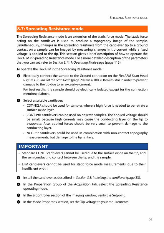
SPREADING RESISTANCE MODE
The Spreading Resistance mode is an extension of the static force mode. The static forceacting on the cantilever is used to produce a topography image of the sample.Simultaneously, changes in the spreading resistance from the cantilever tip to a groundcontact on a sample can be imaged by measuring changes in tip current while a fixedvoltage is applied to the tip. This section gives a brief description of how to operate theFlexAFM in Spreading Resistance mode. For a more detailed description of the parametersthat you can set, refer to Section 8.11.1: Operating Mode page (page 113).
To operate the FlexAFM in the Spreading Resistance mode:
1 Electrically connect the sample to the Ground connector on the FlexAFM Scan Head(Figure 1-3: Parts of the Scan Head (page 20)) via a 100 kOhm resistor in order to preventdamage to the tip due to an excessive current.For best results, the sample should be electrically isolated except for the connectionmentioned above.
2 Select a suitable cantilever:• CDT-NCLR should be used for samples where a high force is needed to penetrate a
surface oxide layer.• CONT-PtIr cantilevers can be used on delicate samples. The applied voltage should
be small, because high currents may cause the conducting layer on the tip toevaporate. Also, applied forces should be very small to prevent damage to theconducting layer.
• NCL-PtIr cantilevers could be used in combination with non-contact topographymeasurements, but damage to the tip is likely.
3 Install the cantilever as described in Section 3.3: Installing the cantilever (page 33).
4 In the Preparation group of the Acquisition tab, select the Spreading Resistanceoperating mode.
5 In the Z-Controller section of the Imaging window, verify the Setpoint.
6 In the Mode Properties section, set the Tip voltage to your requirements.
8.7: Spreading Resistance mode
IMPORTANT• Standard CONTR cantilevers cannot be used due to the surface oxide on the tip, and
the semiconducting contact between the tip and the sample.
• EFM cantilevers cannot be used for static force mode measurements, due to theirinsufficient width.
97
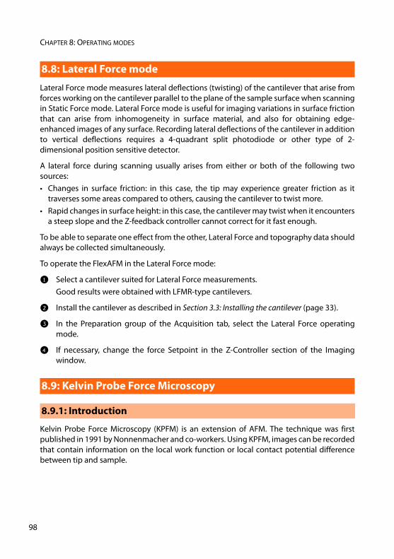
CHAPTER 8: OPERATING MODES
9
Lateral Force mode measures lateral deflections (twisting) of the cantilever that arise fromforces working on the cantilever parallel to the plane of the sample surface when scanningin Static Force mode. Lateral Force mode is useful for imaging variations in surface frictionthat can arise from inhomogeneity in surface material, and also for obtaining edge-enhanced images of any surface. Recording lateral deflections of the cantilever in additionto vertical deflections requires a 4-quadrant split photodiode or other type of 2-dimensional position sensitive detector.
A lateral force during scanning usually arises from either or both of the following twosources: • Changes in surface friction: in this case, the tip may experience greater friction as it
traverses some areas compared to others, causing the cantilever to twist more. • Rapid changes in surface height: in this case, the cantilever may twist when it encounters
a steep slope and the Z-feedback controller cannot correct for it fast enough.
To be able to separate one effect from the other, Lateral Force and topography data shouldalways be collected simultaneously.
To operate the FlexAFM in the Lateral Force mode:
1 Select a cantilever suited for Lateral Force measurements.Good results were obtained with LFMR-type cantilevers.
2 Install the cantilever as described in Section 3.3: Installing the cantilever (page 33).
3 In the Preparation group of the Acquisition tab, select the Lateral Force operatingmode.
4 If necessary, change the force Setpoint in the Z-Controller section of the Imagingwindow.
Kelvin Probe Force Microscopy (KPFM) is an extension of AFM. The technique was firstpublished in 1991 by Nonnenmacher and co-workers. Using KPFM, images can be recordedthat contain information on the local work function or local contact potential differencebetween tip and sample.
8.8: Lateral Force mode
8.9: Kelvin Probe Force Microscopy
8.9.1: Introduction
8
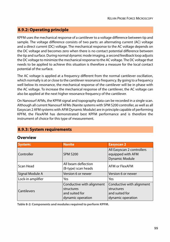
KELVIN PROBE FORCE MICROSCOPY
KPFM uses the mechanical response of a cantilever to a voltage difference between tip andsample. The voltage difference consists of two parts: an alternating current (AC) voltageand a direct current (DC) voltage. The mechanical response to the AC voltage depends onthe DC voltage and becomes zero when there is no contact potential difference betweenthe tip and surface. During normal dynamic mode imaging, a second feedback loop adjuststhe DC voltage to minimize the mechanical response to the AC voltage. The DC voltage thatneeds to be applied to achieve this situation is therefore a measure for the local contactpotential of the surface.
The AC voltage is applied at a frequency different from the normal cantilever oscillation,which normally is at or close to the cantilever resonance frequency. By going to a frequencywell below its resonance, the mechanical response of the cantilever will be in phase withthe AC voltage. To increase the mechanical response of the cantilever, the AC voltage canalso be applied at the next higher resonance frequency of the cantilever.
On Nanosurf AFMs, the KPFM signal and topography data can be recorded in a single scan.Although all current Nanosurf AFMs (Nanite systems with SPM S200 controller, as well as allEasyscan 2 AFM systems with AFM Dynamic Module) are in principle capable of performingKPFM, the FlexAFM has demonstrated best KPFM performance and is therefore theinstrument of choice for this type of measurement.
Overview
8.9.2: Operating principle
8.9.3: System requirements
System: Nanite Easyscan 2
Controller SPM S200All Easyscan 2 controllers equipped with AFM Dynamic Module
Scan HeadAll beam deflection(B-type) scan heads
AFM or FlexAFM
Signal Module A Version 6 or newer Version 6 or newerLock-in amplifier Yes Yes
Cantilevers
Conductive with alignment structuresand suited fordynamic operation
Conductive with alignment structuresand suited fordynamic operation
Table 8-2: Components and modules required to perform KPFM.
99
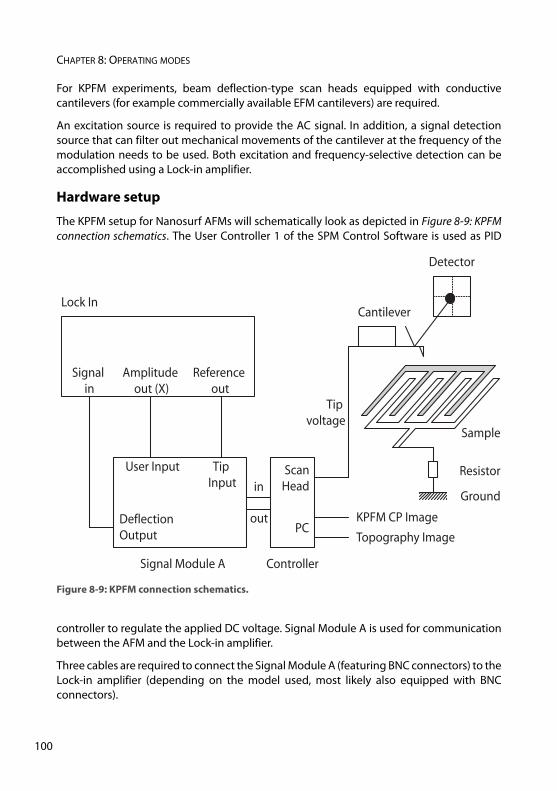
CHAPTER 8: OPERATING MODES
10
For KPFM experiments, beam deflection-type scan heads equipped with conductivecantilevers (for example commercially available EFM cantilevers) are required.
An excitation source is required to provide the AC signal. In addition, a signal detectionsource that can filter out mechanical movements of the cantilever at the frequency of themodulation needs to be used. Both excitation and frequency-selective detection can beaccomplished using a Lock-in amplifier.
Hardware setup
The KPFM setup for Nanosurf AFMs will schematically look as depicted in Figure 8-9: KPFMconnection schematics. The User Controller 1 of the SPM Control Software is used as PID
controller to regulate the applied DC voltage. Signal Module A is used for communicationbetween the AFM and the Lock-in amplifier.
Three cables are required to connect the Signal Module A (featuring BNC connectors) to theLock-in amplifier (depending on the model used, most likely also equipped with BNCconnectors).
Figure 8-9: KPFM connection schematics.
Lock In
Signal in
Amplitude out (X)
Reference out
Cantilever
Sample
Detector
Deflection Output
KPFM CP Image
Topography Image
Tip Input
User Input
Signal Module A Controller
PC
Tip voltage
ScanHead
Resistor
Groundin
out
0
KELVIN PROBE FORCE MICROSCOPY
The reference output of the Lock-in amplifier is used to generate the AC voltage. This wireis connected to the cantilever via the “Tip Voltage” connector on the input side of SignalModule A.
The mechanical response of the cantilever is measured on the cantilever deflectionchannel by connecting “Current or Deflection” on the output side of Signal Module A to the“Signal in” of the Lock-in amplifier.
The X-channel output of the Lock-in is connected to the User 1 connector on the input sideof Signal Module A (see the last sentence of the Lock-in settings section for an explanationas to why the X-channel is used).
If the alternating voltage is applied to the cantilever, the sample has to be grounded.Nanosurf can supply thin cables that can be inserted into the ground connector of the scanhead. A resistor between sample and ground can help prevent short circuits occurringbetween tip and sample.
Alternative setup
Instead of applying the alternating voltage to the cantilever tip, it can also be applied to thesample support. In this case the ground connection has to be removed from the samplesupport and needs to be replaced by a direct connection to the “Reference out” connectorof the Lock-in amplifier, which in turn should no longer be connected to “Tip Voltage” ofSignal Module A.
Lock-in settings
There are several approaches for selecting the reference frequency of the Lock-in: – AC frequency below the resonance frequency of the cantilever
At these low frequencies, the cantilever is in a forced oscillation and the mechanicalresponse of the cantilever and the excitation are almost at the same phase or close to theopposite phase (depending on whether the forces between tip and surface are attractiveor repulsive).
– AC frequency at a higher oscillation mode of the cantileverIn these situations, the cantilever oscillation is self-amplifying.
Note that in both cases, the frequency that can be applied to the tip is limited by a filterpresent in the “Tip Voltage” channel of Signal Module A. The maximum frequency that canbe applied depends on the version number of your Signal Module A.
8.9.4: Procedures
101
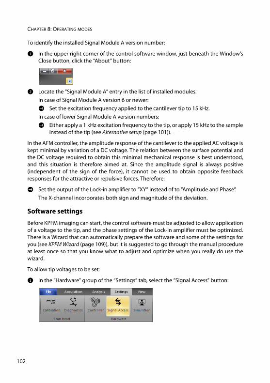
CHAPTER 8: OPERATING MODES
10
To identify the installed Signal Module A version number:
1 In the upper right corner of the control software window, just beneath the Window’sClose button, click the “About” button:
2 Locate the “Signal Module A” entry in the list of installed modules.In case of Signal Module A version 6 or newer:> Set the excitation frequency applied to the cantilever tip to 15 kHz.In case of lower Signal Module A version numbers:> Either apply a 1 kHz excitation frequency to the tip, or apply 15 kHz to the sample
instead of the tip (see Alternative setup (page 101)).
In the AFM controller, the amplitude response of the cantilever to the applied AC voltage iskept minimal by variation of a DC voltage. The relation between the surface potential andthe DC voltage required to obtain this minimal mechanical response is best understood,and this situation is therefore aimed at. Since the amplitude signal is always positive(independent of the sign of the force), it cannot be used to obtain opposite feedbackresponses for the attractive or repulsive forces. Therefore:
> Set the output of the Lock-in amplifier to “XY” instead of to “Amplitude and Phase”.The X-channel incorporates both sign and magnitude of the deviation.
Software settings
Before KPFM imaging can start, the control software must be adjusted to allow applicationof a voltage to the tip, and the phase settings of the Lock-in amplifier must be optimized.There is a Wizard that can automatically prepare the software and some of the settings foryou (see KPFM Wizard (page 109)), but it is suggested to go through the manual procedureat least once so that you know what to adjust and optimize when you really do use thewizard.
To allow tip voltages to be set:
1 In the “Hardware” group of the “Settings” tab, select the “Signal Access” button:
2
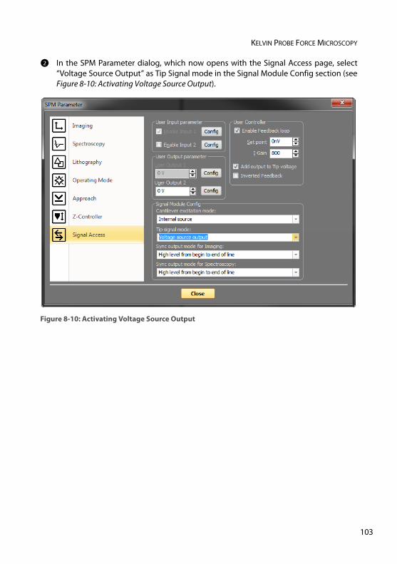
KELVIN PROBE FORCE MICROSCOPY
2 In the SPM Parameter dialog, which now opens with the Signal Access page, select“Voltage Source Output” as Tip Signal mode in the Signal Module Config section (seeFigure 8-10: Activating Voltage Source Output).
Figure 8-10: Activating Voltage Source Output
103
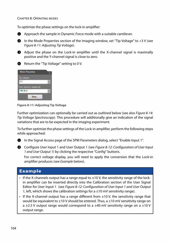
CHAPTER 8: OPERATING MODES
10
To optimize the phase settings on the lock-in amplifier:
1 Approach the sample in Dynamic Force mode with a suitable cantilever.
2 In the Mode Properties section of the Imaging window, set “Tip Voltage” to +3 V (seeFigure 8-11: Adjusting Tip Voltage).
3 Adjust the phase on the Lock-in amplifier until the X-channel signal is maximallypositive and the Y-channel signal is close to zero.
4 Return the “Tip Voltage” setting to 0 V.
Further optimization can optionally be carried out as outlined below (see also Figure 8-14:Tip Voltage Spectroscopy). This procedure will additionally give an indication of the signalvariations that are to be expected in the imaging experiment.
To further optimize the phase settings of the Lock-in amplifier, perform the following stepswhile approached:
1 In the Signal Access page of the SPM Parameters dialog, select “Enable Input 1”.
2 Configure User Input 1 and User Output 1 (see Figure 8-12: Configuration of User Input1 and User Output 1) by clicking the respective “Config” buttons. For correct voltage display, you will need to apply the conversion that the Lock-inamplifier produces (see Example below).
Figure 8-11: Adjusting Tip Voltage
Example• If the X-channels output has a range equal to ±10 V, the sensitivity range of the lock-
in amplifier can be inserted directly into the Calibration section of the User SignalEditor for User Input 1 (see Figure 8-12: Configuration of User Input 1 and User Output1, left, which shows the calibration settings for a ±10 mV sensitivity range).
• If the X-channel output has a range different from ±10 V, the sensitivity range thatwould be equivalent to ±10 V should be entered. Thus, a ±10 mV sensitivity range ona ±2.5 V output range would correspond to a ±40 mV sensitivity range on a ±10 Voutput range.
4
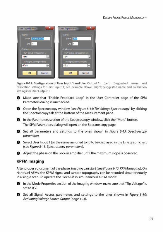
KELVIN PROBE FORCE MICROSCOPY
3 Make sure that “Enable Feedback Loop” in the User Controller page of the SPMParameters dialog is unchecked.
4 Open the Spectroscopy window (see Figure 8-14: Tip Voltage Spectroscopy) by clickingthe Spectroscopy tab at the bottom of the Measurement pane.
5 In the Parameters section of the Spectroscopy window, click the “More” button.The SPM Parameters dialog will open on the Spectroscopy page.
6 Set all parameters and settings to the ones shown in Figure 8-13: Spectroscopyparameters
7 Select User Input 1 (or the name assigned to it) to be displayed in the Line graph chart(see Figure 8-13: Spectroscopy parameters).
8 Adjust the phase on the Lock-in amplifier until the maximum slope is observed.
KPFM Imaging
After proper adjustment of the phase, imaging can start (see Figure 8-15: KPFM imaging). OnNanosurf AFMs, the KPFM signal and sample topography can be recorded simultaneouslyin a single scan. To operate the FlexAFM in simultaneous KPFM mode:
1 In the Mode Properties section of the Imaging window, make sure that “Tip Voltage” isset to 0 V.
2 Set all Signal Access parameters and settings to the ones shown in Figure 8-10:Activating Voltage Source Output (page 103).
Figure 8-12: Configuration of User Input 1 and User Output 1. (Left) Suggested name andcalibration settings for User Input 1; see example above. (Right) Suggested name and calibrationsettings for User Output 1.
105
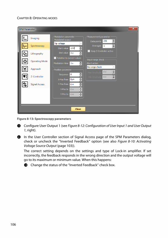
CHAPTER 8: OPERATING MODES
10
3 Configure User Output 1 (see Figure 8-12: Configuration of User Input 1 and User Output1, right).
4 In the User Controller section of Signal Access page of the SPM Parameters dialog,check or uncheck the “Inverted Feedback” option (see also Figure 8-10: ActivatingVoltage Source Output (page 103)).The correct setting depends on the settings and type of Lock-in amplifier. If setincorrectly, the feedback responds in the wrong direction and the output voltage willgo to its maximum or minimum value. When this happens:> Change the status of the “Inverted Feedback” check box.
Figure 8-13: Spectroscopy parameters
6
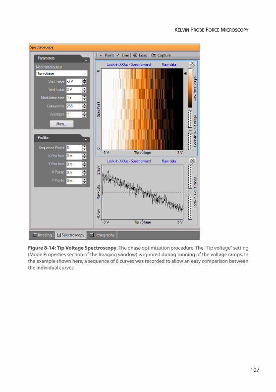
KELVIN PROBE FORCE MICROSCOPY
Figure 8-14: Tip Voltage Spectroscopy. The phase optimization procedure. The “Tip voltage” setting(Mode Properties section of the Imaging window) is ignored during running of the voltage ramps. Inthe example shown here, a sequence of 8 curves was recorded to allow an easy comparison betweenthe individual curves.
107
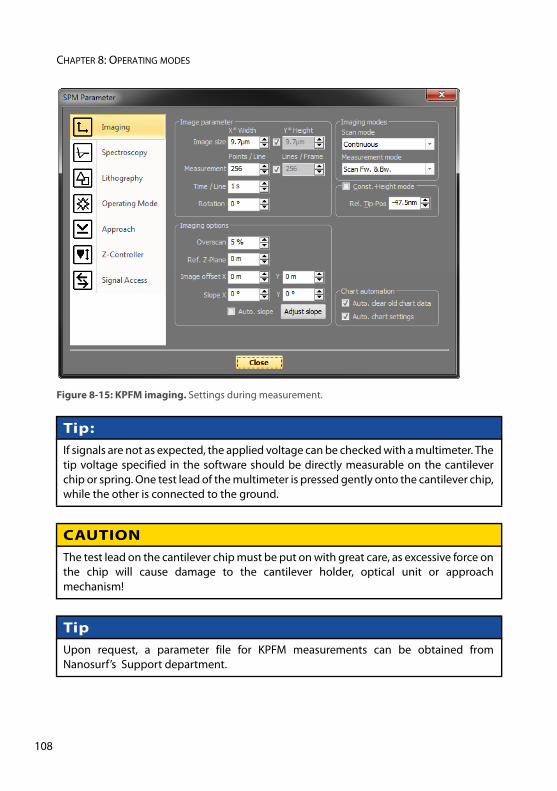
CHAPTER 8: OPERATING MODES
10
Figure 8-15: KPFM imaging. Settings during measurement.
Tip: If signals are not as expected, the applied voltage can be checked with a multimeter. Thetip voltage specified in the software should be directly measurable on the cantileverchip or spring. One test lead of the multimeter is pressed gently onto the cantilever chip,while the other is connected to the ground.
CAUTIONThe test lead on the cantilever chip must be put on with great care, as excessive force onthe chip will cause damage to the cantilever holder, optical unit or approachmechanism!
TipUpon request, a parameter file for KPFM measurements can be obtained fromNanosurf’s Support department.
8
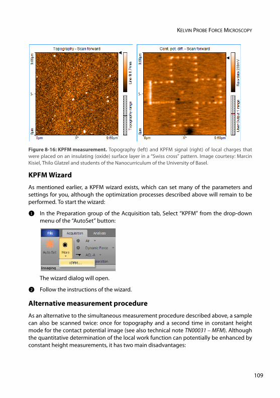
KELVIN PROBE FORCE MICROSCOPY
KPFM Wizard
As mentioned earlier, a KPFM wizard exists, which can set many of the parameters andsettings for you, although the optimization processes described above will remain to beperformed. To start the wizard:
1 In the Preparation group of the Acquisition tab, Select “KPFM” from the drop-downmenu of the “AutoSet” button:
The wizard dialog will open.
2 Follow the instructions of the wizard.
Alternative measurement procedure
As an alternative to the simultaneous measurement procedure described above, a samplecan also be scanned twice: once for topography and a second time in constant heightmode for the contact potential image (see also technical note TN00031 – MFM). Althoughthe quantitative determination of the local work function can potentially be enhanced byconstant height measurements, it has two main disadvantages:
Figure 8-16: KPFM measurement. Topography (left) and KPFM signal (right) of local charges thatwere placed on an insulating (oxide) surface layer in a “Swiss cross” pattern. Image courtesy: MarcinKisiel, Thilo Glatzel and students of the Nanocurriculum of the University of Basel.
109
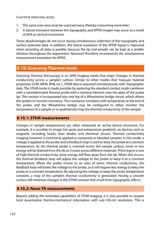
CHAPTER 8: OPERATING MODES
11
1. The same scan area must be scanned twice, thereby consuming more time.2. A lateral mismatch between the topography and KPFM images may occur as a result
of drift or vertical movement.
These disadvantages do not occur during simultaneous collection of the topography andsurface potential data. In addition, the lateral resolution of the KPFM signal is improvedwhen recording all data in parallel, because the tip and sample can be kept at a smallerdistance throughout the experiment. Nanosurf therefore recommends the simultaneousmeasurement procedure for KPFM.
Scanning Thermal Microscopy is an AFM imaging mode that maps changes in thermalconductivity across a sample’s surface. Similar to other modes that measure materialproperties (LFM, MFM, EFM, etc.), SThM data is acquired simultaneously with Topographicdata. The SThM mode is made possible by replacing the standard contact mode cantileverwith a nanofabricated thermal probe with a resistive element near the apex of the probetip. This resistor is incorporated into one leg of a Wheatstone bridge circuit, which allowsthe system to monitor resistance. This resistance correlates with temperature at the end ofthe probe, and the Wheatstone bridge may be configured to either monitor thetemperature of a sample or to qualitatively map the thermal conductivity of the sample.
Changes in sample temperatures are often measured on active device structures. Forexample, it is possible to image hot spots and temperature gradients on devices such asmagnetic recording heads, laser diodes, and electrical circuits. Thermal conductivityimaging, however, is commonly applied to composite or blended samples. In this mode, avoltage is applied to the probe and a feedback loop is used to keep the probe at a constanttemperature. As the thermal probe is scanned across the sample surface, more or lessenergy will be drained from the tip as it scans across different materials. If the region is oneof high thermal conductivity, more energy will flow away from the tip. When this occurs,the thermal feedback loop will adjust the voltage to the probe to keep it at a constanttemperature. When the probe moves to an area of lower thermal conductivity, thefeedback loop will lower the voltage to the probe, as it will require less energy to keep theprobe at a constant temperature. By adjusting the voltage to keep the probe temperatureconstant, a map of the sample’s thermal conductivity is generated. Having a smoothsurface will minimize changes in the SThM contrast that result from topographic effects.
Beyond adding the extended capabilities of SThM imaging, it is also possible to acquirelocal quantitative thermo-mechanical information with sub-100-nm resolution. This is
8.10: Scanning Thermal mode
8.10.1: SThM measurements
8.10.2: Nano-TA measurements
0
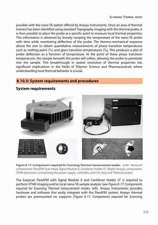
SCANNING THERMAL MODE
possible with the nano-TA option offered by Anasys Instruments. Once an area of thermalinterest has been identified using standard Topography imaging with the thermal probe, itis then possible to place the probe at a specific point to measure local thermal properties.This information is obtained by linearly ramping the temperature of the nano-TA probewith time while monitoring deflection of the probe. The thermo-mechanical responseallows the user to obtain quantitative measurements of phase transition temperaturessuch as melting point (Tm) and glass transition temperatures (Tg). This produces a plot ofprobe deflection as a function of temperature. At the point of these phase transitiontemperatures, the sample beneath the probe will soften, allowing the probe to penetrateinto the sample. This breakthrough in spatial resolution of thermal properties hassignificant implications in the fields of Polymer Science and Pharmaceuticals whereunderstanding local thermal behavior is crucial.
System requirements
The Easyscan FlexAFM with Signal Module A and Cantilever Holder ST is required toperform SThM imaging and/or local nano-TA sample analysis (see Figure 8-17: Componentsrequired for Scanning Thermal measurement modes, left). Anasys Instruments provideshardware and software that easily integrate with the FlexAFM system. Anasys thermalprobes are premounted on supports (Figure 8-17: Components required for Scanning
8.10.3: System requirements and procedures
Figure 8-17: Components required for Scanning Thermal measurement modes. (Left) Nanosurfcomponents: FlexAFM Scan Head, Signal Module A, Cantilever Holder ST. (Right) Anasys components:SThM electronics (comprising the power supply, controller, and CAL box) and Thermal probes
111
CHAPTER 8: OPERATING MODES
11
Thermal measurement modes, right) that are compatible with the FlexAFM CantileverHolder ST. The Anasys SThM system (Figure 8-17: Components required for Scanning Thermalmeasurement modes, right) includes a simple software interface that controls the thermalanalysis electronics via a USB connection. This interface is capable of outputting a low-noise, high-resolution voltage to the probe. The voltage may be varied over a wide rangedepending on the probe type and the desired temperature of the probe (<0.1°Cresolution). The other components in the bridge circuit are easily changed if required forcustom experiments, and the system includes an input connection to apply AC voltages tothe probe. The resistance of the probe is output on a BNC, which is then connected to UserInput 1 on the Easyscan 2 Signal Module A. For SThM imaging, the control software isconfigured to collect the resistance data on User Input 1, allowing SThM information to berecorded and displayed as a chart in the imaging window of the control software. Duringnano-TA experiments, the Anasys software allows the User to set Nano-TA2 controllerparameters such as heating rates and temperature range. Typically, AFM feedback is turnedoff during the acquisition of nano-TA data.
Procedures
To operate the FlexAFM in the Scanning Thermal mode:
1 Set up the hardware as described in Technical Note “TN00475 — How to operate theEasyscan 2 FlexAFM with Anasys thermal probes” (contact Nanosurf Support fordetails). Good results were obtained with Anasys GLA-1 and AN2-200 probes.
2 In the Preparation group of the Acquisition tab, select the Dynamic Force operatingmode.
3 Set the Z-Controller parameters to appropriate values for the measurement.
4 In the “User Input parameter” section of the Signal Access page of the SPM Parametersdialog (opened by clicking the “More” button in any of the section of the Imagingwindow), check the “Enable User Input 1” checkbox.
5 Configure User Input 1 as required (see Section 14.9: User Signal Editor dialog (page263)).
2
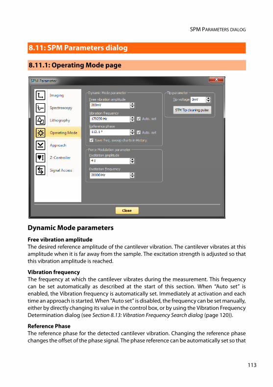
SPM PARAMETERS DIALOG
Dynamic Mode parameters
Free vibration amplitude The desired reference amplitude of the cantilever vibration. The cantilever vibrates at thisamplitude when it is far away from the sample. The excitation strength is adjusted so thatthis vibration amplitude is reached.
Vibration frequencyThe frequency at which the cantilever vibrates during the measurement. This frequencycan be set automatically as described at the start of this section. When “Auto set” isenabled, the Vibration frequency is automatically set. Immediately at activation and eachtime an approach is started. When “Auto set” is disabled, the frequency can be set manually,either by directly changing its value in the control box, or by using the Vibration FrequencyDetermination dialog (see Section 8.13: Vibration Frequency Search dialog (page 120)).
Reference Phase The reference phase for the detected cantilever vibration. Changing the reference phasechanges the offset of the phase signal. The phase reference can be automatically set so that
8.11: SPM Parameters dialog
8.11.1: Operating Mode page
113
CHAPTER 8: OPERATING MODES
11
the phase signal is zero. When “Auto set” is enabled the phase reference is automatically setafter finishing the approach.
Force Modulation parameters
Excitation amplitude The amplitude of the sensor excitation during a force modulation mode measurement.
Excitation frequency The frequency of the sensor excitation during a force modulation mode measurement.
Tip Parameter
Tip Voltage This parameter defines the potential to be applied to the tip. The voltage that can be usedlies between -10V and +10V.
Info:With the STM scan head the sample is automatically connected to the ground of theinstrument. With AFM scan heads the sample has to be electrically connected to theinstrument chassis ground for accurate measurements.
4
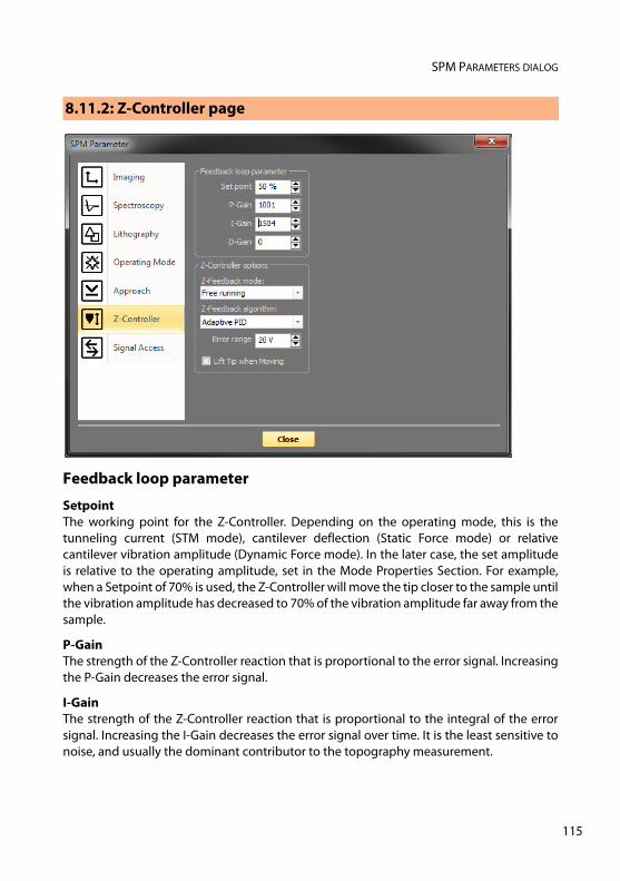
SPM PARAMETERS DIALOG
Feedback loop parameter
SetpointThe working point for the Z-Controller. Depending on the operating mode, this is thetunneling current (STM mode), cantilever deflection (Static Force mode) or relativecantilever vibration amplitude (Dynamic Force mode). In the later case, the set amplitudeis relative to the operating amplitude, set in the Mode Properties Section. For example,when a Setpoint of 70% is used, the Z-Controller will move the tip closer to the sample untilthe vibration amplitude has decreased to 70% of the vibration amplitude far away from thesample.
P-Gain The strength of the Z-Controller reaction that is proportional to the error signal. Increasingthe P-Gain decreases the error signal.
I-Gain The strength of the Z-Controller reaction that is proportional to the integral of the errorsignal. Increasing the I-Gain decreases the error signal over time. It is the least sensitive tonoise, and usually the dominant contributor to the topography measurement.
8.11.2: Z-Controller page
115
CHAPTER 8: OPERATING MODES
11
D-Gain The strength of the Z-Controller reaction that is proportional to the derivative of the errorsignal. Increasing the D-Gain decreases fast changes in the error signal, but also amplifieshigh frequency noise.
Z-Controller options
Z-Feedback Mode The following modes are available: – Free Running
The Z-Controller is active. – Freeze Position
The Z-Controller is not active, the scanner remains in its current Z-position. – Stop and Clear
The Z-Controller is not active, the scanner is moved to the “Ref. Z Plane”, set in theImaging page of the SPM Parameters dialog. The Probe Status Light will blink green aslong as the Z-Controller is deactivated.
Z-Feedback algorithm The following algorithms are available: – Standard PID
A standard PID controller is used for Z-Feedback. – Adaptive PID
A standard PID controller is used for Z-feedback. In addition, the bandwidth of theTopography measurement is adapted to the number of measured points per second. Theadaptive PID controller thus reduces noise in the measurement. However, topographychanges that happen faster than the time between two measured points are also lost.This makes it more difficult to detect vibrations due to instability of the feedback loop.These vibrations remain visible in the Current, Amplitude, or Deflection signal, however,so always monitor these signals when optimizing Z-Controller settings, especially whenusing the Adaptive PID.
Error Range The range of the error signal used to control the Z-Position. The error signal is the differencebetween the signal used for topography feedback and the current Setpoint. When thevalue of “Error Range” is reduced, the resolution of the error signal is increased.
CAUTIONThe tip may be damaged when the Z-Controller is not active during scanning. This willhappen when Ref. Z Plane is much lower than the current position of the tip, or whenthe scan range contains large height differences.
6
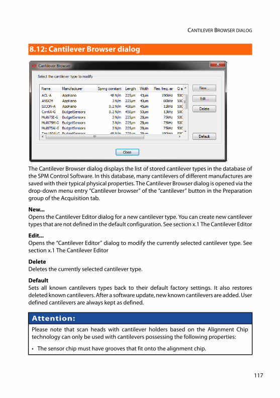
CANTILEVER BROWSER DIALOG
The Cantilever Browser dialog displays the list of stored cantilever types in the database ofthe SPM Control Software. In this database, many cantilevers of different manufactures aresaved with their typical physical properties. The Cantilever Browser dialog is opened via thedrop-down menu entry “Cantilever browser” of the “cantilever” button in the Preparationgroup of the Acquisition tab.
New... Opens the Cantilever Editor dialog for a new cantilever type. You can create new cantilevertypes that are not defined in the default configuration. See section x.1 The Cantilever Editor
Edit...Opens the “Cantilever Editor” dialog to modify the currently selected cantilever type. Seesection x.1 The Cantilever Editor
Delete Deletes the currently selected cantilever type.
Default Sets all known cantilevers types back to their default factory settings. It also restoresdeleted known cantilevers. After a software update, new known cantilevers are added. Userdefined cantilevers are always kept as defined.
8.12: Cantilever Browser dialog
Attention:Please note that scan heads with cantilever holders based on the Alignment Chiptechnology can only be used with cantilevers possessing the following properties:
• The sensor chip must have grooves that fit onto the alignment chip.
117
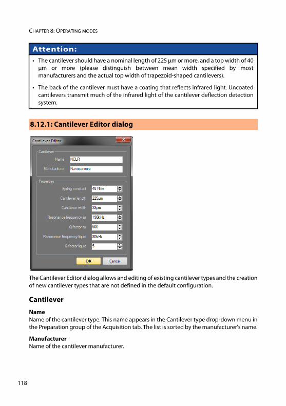
CHAPTER 8: OPERATING MODES
11
The Cantilever Editor dialog allows and editing of existing cantilever types and the creationof new cantilever types that are not defined in the default configuration.
Cantilever
NameName of the cantilever type. This name appears in the Cantilever type drop-down menu inthe Preparation group of the Acquisition tab. The list is sorted by the manufacturer's name.
ManufacturerName of the cantilever manufacturer.
• The cantilever should have a nominal length of 225 μm or more, and a top width of 40μm or more (please distinguish between mean width specified by mostmanufacturers and the actual top width of trapezoid-shaped cantilevers).
• The back of the cantilever must have a coating that reflects infrared light. Uncoatedcantilevers transmit much of the infrared light of the cantilever deflection detectionsystem.
8.12.1: Cantilever Editor dialog
Attention:
8
CANTILEVER BROWSER DIALOG
Properties
Spring constant This parameter defines the nominal spring constant of the cantilever type. This value isused to calculate the correct force used for Z-Controller Setpoint and chart signals in alloperating modes that use the Static Force for Z-control.
Cantilever length The nominal length of this cantilever type (for information only, currently not used by thecontrol software).
Cantilever width The mean width of this cantilever type (for information only, currently not used by thecontrol software).
Resonance frequency air / Resonance frequency liquidThe nominal resonance frequency of the cantilever type in air or in liquid measurementenvironment. This frequency is used for calculation of the automatic coarse frequencysweep search range (see Section 8.13: Vibration Frequency Search dialog (page 120)).
Q-factor air / Q-factor liquid The apparent quality factor of the cantilever in air or in liquid measurement environment.The higher the number, the sharper the peak. By default, this number is 500 in air and 5 inliquid. The quality factor is used for calculation of the automatic fine frequency sweepsearch range (see Section 8.13: Vibration Frequency Search dialog (page 120)).
IMPORTANTThe deflection calibration value of the current scan head calibration file is used tocalculate the force:
Force [N] = Spring Constant [N/m] * Deflection [m]
119
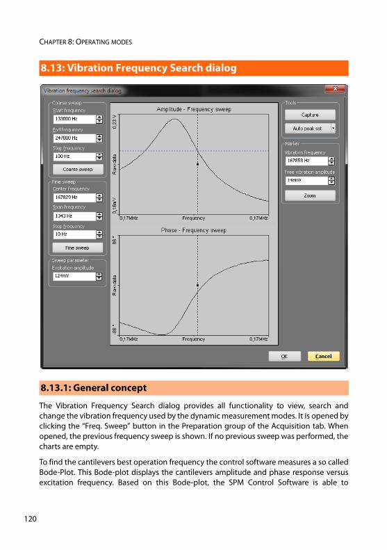
CHAPTER 8: OPERATING MODES
12
The Vibration Frequency Search dialog provides all functionality to view, search andchange the vibration frequency used by the dynamic measurement modes. It is opened byclicking the “Freq. Sweep” button in the Preparation group of the Acquisition tab. Whenopened, the previous frequency sweep is shown. If no previous sweep was performed, thecharts are empty.
To find the cantilevers best operation frequency the control software measures a so calledBode-Plot. This Bode-plot displays the cantilevers amplitude and phase response versusexcitation frequency. Based on this Bode-plot, the SPM Control Software is able to
8.13: Vibration Frequency Search dialog
8.13.1: General concept
0
VIBRATION FREQUENCY SEARCH DIALOG
automatically detect the cantilever resonance peak and adjust the operating frequencyaccordingly. In some cases (mostly in Liquid environment) it is necessary for the user toadjust the operating frequency manually (based on the Bode-plot result), because theautomatic algorithm is not able to find the right frequency peak.
For recording the Bode-plot, the SPM Control Software tunes the cantilever excitation froma start frequency slowly up to a higher frequency. During this tuning (or sweeping) thecantilevers amplitude and phase response is measured and saved. The result is plotted inan Amplitude and a Phase versus Frequency chart. The Excitation amplitude is heldconstant during the sweep. Therefore, any change in detector amplitude and phase signalis a result of cantilever response.
Resonance frequencies vary greatly between cantilevers, depending on the cantilever’srespective physical properties. Cantilever manufacturers provide information on theresonance frequency range of each cantilever type. The SPM Control Software thereforehas a built-in database of commonly used cantilevers. Other cantilever can be manuallyadded by the user (see Section 8.12: Cantilever Browser dialog (page 117)). Based on thisdatabase information, the control software selects the frequency sweep range.
After a coarse and a fine sweep, the optimal operating frequency is chosen close to theresonance frequency of the cantilever.
Tools
Auto frequency setA click to this button starts an automated vibration frequency peak search andoptimization procedure. This procedure consists of four phases: 1. First a coarse frequency sweep based on the database information of the currently
selected cantilever is performed. The frequency range of this sweep is shown in thecoarse sweep section.
2. Based on the best frequency peak found in this coarse sweep a narrow band finesweep is done. The frequency peak and sweep range used for the fine sweep is shownin the fine sweep section.
3. Based on the amplitude reduction settings (accessed by choosing “Config...” from the“Auto frequency set” buttons drop-down menu) the optimal vibration frequency is
IMPORTANTThe Phase measurement and chart plot is performed only if a Mode Extension Moduleis installed in the SPM controller. The Phase is always measured, independent on theselected Operating Mode.
8.13.2: Automated vibration frequency search
121
CHAPTER 8: OPERATING MODES
12
selected and the excitation amplitude tuned to get the desired free vibrationamplitude at this frequency.
4. After the amplitude tuning, a final fine sweep is performed with the new excitationamplitude.
At the end of the procedure, the new operating frequency is shown by the marker (bothgraphically and in numbers). Additionally, the “excitation amplitude” parameter shows theamplitude required to obtain the desired free vibration amplitude.
The user may now just leave the dialog and accept the new frequency using the “OK”button, reset to previous values with the “Cancel” button, do manual adjustment with themarker, or change amplitude settings and/or customize frequency sweep ranges throughuse of the edit boxes and action buttons.
CaptureStores a copy of the current Bode-plot in the History page of the Gallery panel. The data isstored as a new measurement and remains open in the Document space of the SPMControl Software.
Config...Selected from the “Auto frequency set” button’s drop-down menu, this menu option opensthe Auto frequency config dialog (see Section 8.13.4: Auto Frequency Config dialog (page124)).
Marker
The marker represents the currently selected frequency. It is shown as a dotted vertical linein the amplitude and phase chart. The corresponding “Vibration frequency” and “Freevibration amplitude” values (see below) are shown as automatically updating numbers inthe Vibration frequency and Free vibration amplitude edit boxes as well.
To move the marker by mouse, click and hold the line's handle (small black box in the centerof the line) and move it around. The vibration frequency is updated immediately during themovement. At release of the marker the amplitude is measured and drawn as a horizontalline in the amplitude chart and its value is displayed in the Free vibration amplitude editbox.
To use the currently shown frequency as the new vibration frequency, leave the dialog withthe “OK” button.
Vibration frequency This parameter shows the frequency at the marker's position. It is used as the actualvibration frequency during operation of the microscope in the Dynamic operating modes.The value of this frequency can be changed manually by typing in the desired value, by
8.13.3: Manual sweep controls
2
VIBRATION FREQUENCY SEARCH DIALOG
using the arrow keys beside the parameter field, or by dragging the frequency marker linein the charts as described above.
Free vibration amplitude This parameter shows the actual amplitude at the current marker frequency. If the userenters a new value, the excitation amplitude is adjusted to obtain a free cantileveramplitude with this new value. A new frequency sweep is immediately performed and itsresults displayed. If the desired amplitude could not be set, an error dialog is shown.
Zoom A click on this button starts a new frequency sweep with a smaller frequency range thancurrently displayed in the charts. The center of the sweep is at the markers position. Thenew sweep range and center position is shown in the Fine sweep parameter section.
Coarse sweep
Start / End FrequencyThese parameters defines the sweep range of a coarse frequency sweep. This range isnormally set large enough to search for the initial resonance peak. “Auto frequency set”sets these parameters to the range found in the Cantilever database for the currentlyselected cantilever.
Step FrequencyThis parameter defines the frequency steps used during the sweep. Therefore, the numberof data points of the sweep is defined as:
Datapoint = (End – Start) / Step.
Typical step sizes during a coarse sweep are 100 Hz or more.
Coarse s weepThe “Coarse sweep” button performs a coarse frequency sweep according to the coarsesweep parameters entered (see above).
Fine sweep section
Center / Span FrequencyThese parameters defines the sweep range of a fine frequency sweep. The range isnormally smaller than the coarse sweep range. “Auto frequency set” sets the centerfrequency to the resonance peak found during the coarse sweep. The span is set accordingto the quality factor found in the Cantilever database for the currently selected cantilever.Span defines the start and end frequencies for the fine sweep as follows:
123
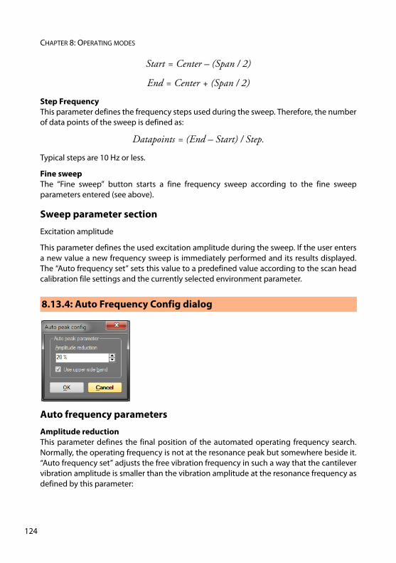
CHAPTER 8: OPERATING MODES
12
Start = Center – (Span / 2)
End = Center + (Span / 2)
Step FrequencyThis parameter defines the frequency steps used during the sweep. Therefore, the numberof data points of the sweep is defined as:
Datapoints = (End – Start) / Step.
Typical steps are 10 Hz or less.
Fine sweepThe “Fine sweep” button starts a fine frequency sweep according to the fine sweepparameters entered (see above).
Sweep parameter section
Excitation amplitude
This parameter defines the used excitation amplitude during the sweep. If the user entersa new value a new frequency sweep is immediately performed and its results displayed.The “Auto frequency set” sets this value to a predefined value according to the scan headcalibration file settings and the currently selected environment parameter.
Auto frequency parameters
Amplitude reductionThis parameter defines the final position of the automated operating frequency search.Normally, the operating frequency is not at the resonance peak but somewhere beside it.“Auto frequency set” adjusts the free vibration frequency in such a way that the cantilevervibration amplitude is smaller than the vibration amplitude at the resonance frequency asdefined by this parameter:
8.13.4: Auto Frequency Config dialog
4
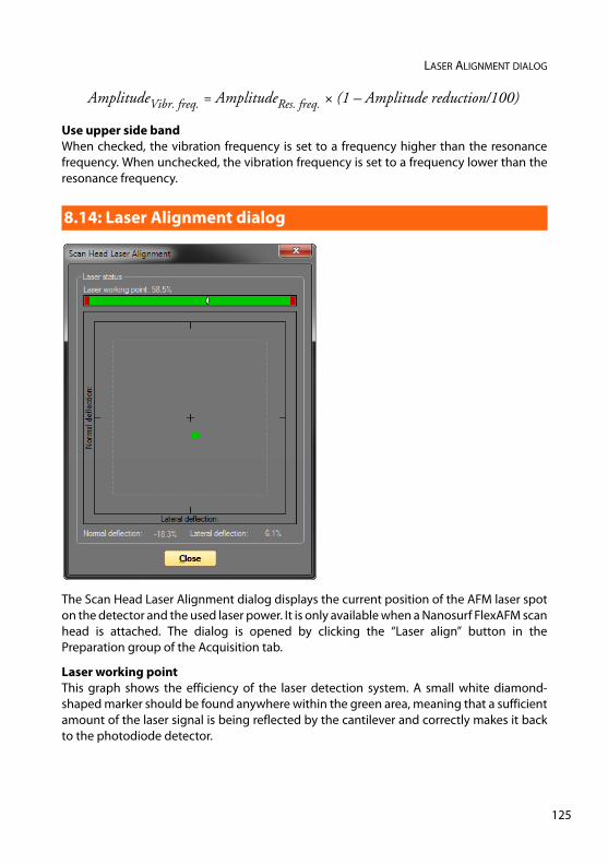
LASER ALIGNMENT DIALOG
AmplitudeVibr. freq. = AmplitudeRes. freq. × (1 – Amplitude reduction/100)
Use upper side band When checked, the vibration frequency is set to a frequency higher than the resonancefrequency. When unchecked, the vibration frequency is set to a frequency lower than theresonance frequency.
The Scan Head Laser Alignment dialog displays the current position of the AFM laser spoton the detector and the used laser power. It is only available when a Nanosurf FlexAFM scanhead is attached. The dialog is opened by clicking the “Laser align” button in thePreparation group of the Acquisition tab.
Laser working point This graph shows the efficiency of the laser detection system. A small white diamond-shaped marker should be found anywhere within the green area, meaning that a sufficientamount of the laser signal is being reflected by the cantilever and correctly makes it backto the photodiode detector.
8.14: Laser Alignment dialog
125
CHAPTER 8: OPERATING MODES
12
If the marker resides in the red area to the right, it will turn red too, signaling that too littlelaser light is being detected. This can be caused by a misaligned cantilever, or by somethingblocking the optical path of the laser.
If the marker resides in the red area to the left, too much light is being detected by thephotodiode detector, usually caused by strong environmental light. This condition is veryrare, however.
Laser position This graphical area shows where the deflected laser beam hits the photodiode detector. Agreen spot anywhere within the area enclosed by the dotted square means that thecantilever deflection detection system (consisting of laser, cantilever, and detector) isproperly aligned. If the laser spot falls outside this area, it will become red, meaning thatthe alignment does not allow proper measurements to take place. Usually this is caused bya misaligned cantilever, which can be easily corrected. The position of the laser spot is alsogiven as a percentage of the maximum deflection the detector can identify.
6

CHAPTER 9:
Positioning0
0
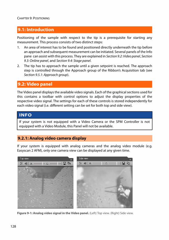
CHAPTER 9: POSITIONING
12
Positioning of the sample with respect to the tip is a prerequisite for starting anymeasurement. This process consists of two distinct steps:1. An area of interest has to be found and positioned directly underneath the tip before
an approach and subsequent measurement can be initiated. Several panels of the Infopane can assist with this process. They are explained in Section 9.2: Video panel, Section9.3: Online panel, and Section 9.4: Stage panel.
2. The tip has to approach the sample until a given setpoint is reached. The approachstep is controlled through the Approach group of the Ribbon’s Acquisition tab (seeSection 9.5.1: Approach group).
The Video panel displays the available video signals. Each of the graphical sections used forthis contains a toolbar with control options to adjust the display properties of therespective video signal. The settings for each of these controls is stored independently foreach video signal (i.e. different setting can be set for both top and side view).
If your system is equipped with analog cameras and the analog video module (e.g.Easyscan 2 AFM), only one camera view can be displayed at any given time.
9.1: Introduction
9.2: Video panel
INFOIf your system is not equipped with a Video Camera or the SPM Controller is notequipped with a Video Module, this Panel will not be available.
9.2.1: Analog video camera display
Figure 9-1: Analog video signal in the Video panel. (Left) Top view. (Right) Side view.
8
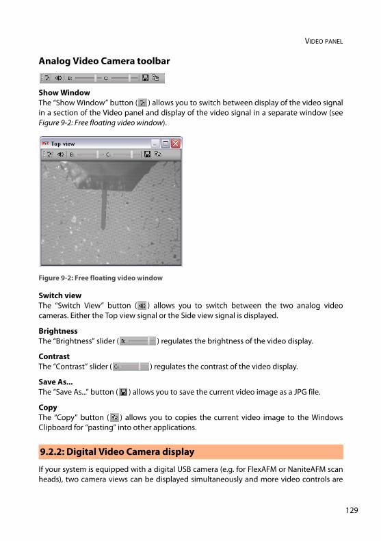
VIDEO PANEL
Analog Video Camera toolbar
Show WindowThe “Show Window” button ( ) allows you to switch between display of the video signalin a section of the Video panel and display of the video signal in a separate window (seeFigure 9-2: Free floating video window).
Switch viewThe “Switch View” button ( ) allows you to switch between the two analog videocameras. Either the Top view signal or the Side view signal is displayed.
BrightnessThe “Brightness” slider ( ) regulates the brightness of the video display.
ContrastThe “Contrast” slider ( ) regulates the contrast of the video display.
Save As... The “Save As...” button ( ) allows you to save the current video image as a JPG file.
CopyThe “Copy” button ( ) allows you to copies the current video image to the WindowsClipboard for “pasting” into other applications.
If your system is equipped with a digital USB camera (e.g. for FlexAFM or NaniteAFM scanheads), two camera views can be displayed simultaneously and more video controls are
Figure 9-2: Free floating video window
9.2.2: Digital Video Camera display
129
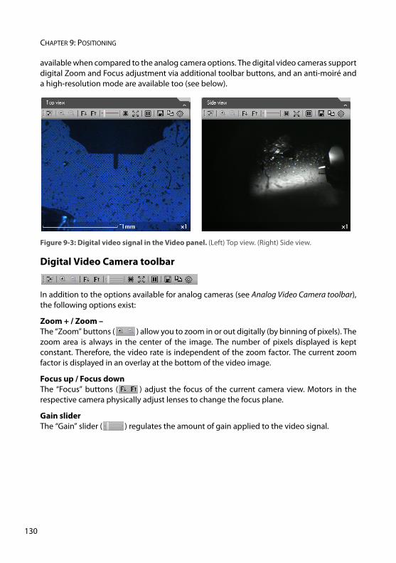
CHAPTER 9: POSITIONING
13
available when compared to the analog camera options. The digital video cameras supportdigital Zoom and Focus adjustment via additional toolbar buttons, and an anti-moiré anda high-resolution mode are available too (see below).
Digital Video Camera toolbar
In addition to the options available for analog cameras (see Analog Video Camera toolbar),the following options exist:
Zoom + / Zoom –The “Zoom” buttons ( ) allow you to zoom in or out digitally (by binning of pixels). Thezoom area is always in the center of the image. The number of pixels displayed is keptconstant. Therefore, the video rate is independent of the zoom factor. The current zoomfactor is displayed in an overlay at the bottom of the video image.
Focus up / Focus downThe “Focus” buttons ( ) adjust the focus of the current camera view. Motors in therespective camera physically adjust lenses to change the focus plane.
Gain sliderThe “Gain” slider ( ) regulates the amount of gain applied to the video signal.
Figure 9-3: Digital video signal in the Video panel. (Left) Top view. (Right) Side view.
0
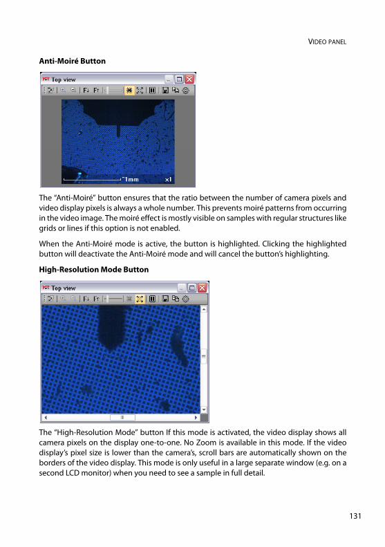
VIDEO PANEL
Anti-Moiré Button
The “Anti-Moiré” button ensures that the ratio between the number of camera pixels andvideo display pixels is always a whole number. This prevents moiré patterns from occurringin the video image. The moiré effect is mostly visible on samples with regular structures likegrids or lines if this option is not enabled.
When the Anti-Moiré mode is active, the button is highlighted. Clicking the highlightedbutton will deactivate the Anti-Moiré mode and will cancel the button’s highlighting.
High-Resolution Mode Button
The “High-Resolution Mode” button If this mode is activated, the video display shows allcamera pixels on the display one-to-one. No Zoom is available in this mode. If the videodisplay’s pixel size is lower than the camera’s, scroll bars are automatically shown on theborders of the video display. This mode is only useful in a large separate window (e.g. on asecond LCD monitor) when you need to see a sample in full detail.
131
CHAPTER 9: POSITIONING
13
When the High Resolution mode is active, the button is highlighted. Clicking thehighlighted button will deactivate the High-Resolution mode and will cancel the button’shighlighting.
Pause ButtonIf the “Pause” button ( ) is activated the video image update is stopped and the frozenimage (last frame received) is shown continuously. A second click on this button restartsthe real time video display.
Video Properties ButtonA click on this button opens the Digital Video Properties Dialog. See the next section(Section 9.2.4: Digital Video Properties dialog) for details.
The Illumination section of the Video panel contains an Illumination slider that controls theintensity of the sample illumination LED. It may be used to adjust the amount of light onthe sample, thereby optimizing the video image.
If you have an analog camera installed in your system, the illumination settings will dependon the selected camera view (top or side view) and will be stored individually.
In case you have a digital camera in your system, where top and side view are shownsimultaneously, only one illumination setting is used.
If no camera is installed, the Video panel will not be accessible, and the Illumination sliderwill therefore be present in the Online panel (see Section 9.3.3: Illumination section).
IMPORTANTIn high-resolution mode the amount of (video pixel) data that needs to be transferredover the USB connection is huge. As a result, the video frame rate typically drops below5 Hz and a high-performance PC is required to keep the system stable.
9.2.3: Illumination section
2
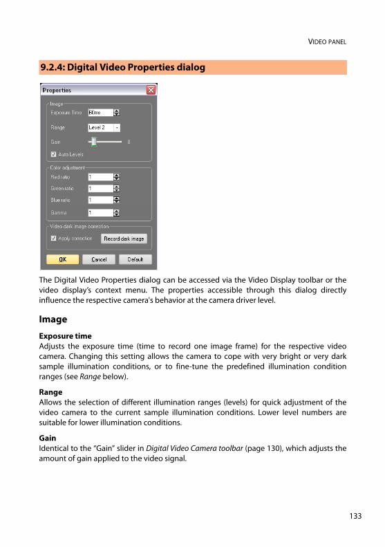
VIDEO PANEL
The Digital Video Properties dialog can be accessed via the Video Display toolbar or thevideo display’s context menu. The properties accessible through this dialog directlyinfluence the respective camera's behavior at the camera driver level.
Image
Exposure timeAdjusts the exposure time (time to record one image frame) for the respective videocamera. Changing this setting allows the camera to cope with very bright or very darksample illumination conditions, or to fine-tune the predefined illumination conditionranges (see Range below).
RangeAllows the selection of different illumination ranges (levels) for quick adjustment of thevideo camera to the current sample illumination conditions. Lower level numbers aresuitable for lower illumination conditions.
GainIdentical to the “Gain” slider in Digital Video Camera toolbar (page 130), which adjusts theamount of gain applied to the video signal.
9.2.4: Digital Video Properties dialog
133
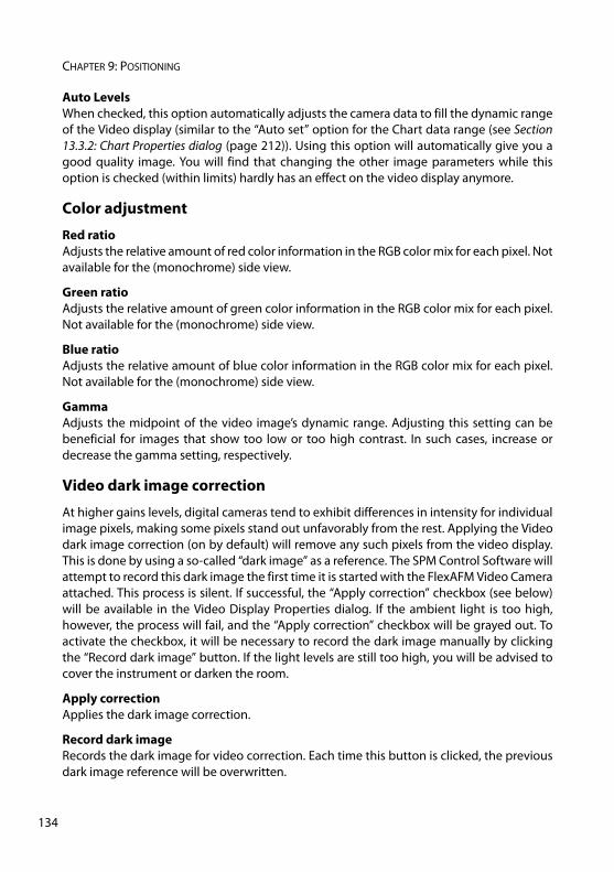
CHAPTER 9: POSITIONING
13
Auto LevelsWhen checked, this option automatically adjusts the camera data to fill the dynamic rangeof the Video display (similar to the “Auto set” option for the Chart data range (see Section13.3.2: Chart Properties dialog (page 212)). Using this option will automatically give you agood quality image. You will find that changing the other image parameters while thisoption is checked (within limits) hardly has an effect on the video display anymore.
Color adjustment
Red ratioAdjusts the relative amount of red color information in the RGB color mix for each pixel. Notavailable for the (monochrome) side view.
Green ratioAdjusts the relative amount of green color information in the RGB color mix for each pixel.Not available for the (monochrome) side view.
Blue ratioAdjusts the relative amount of blue color information in the RGB color mix for each pixel.Not available for the (monochrome) side view.
GammaAdjusts the midpoint of the video image’s dynamic range. Adjusting this setting can bebeneficial for images that show too low or too high contrast. In such cases, increase ordecrease the gamma setting, respectively.
Video dark image correction
At higher gains levels, digital cameras tend to exhibit differences in intensity for individualimage pixels, making some pixels stand out unfavorably from the rest. Applying the Videodark image correction (on by default) will remove any such pixels from the video display.This is done by using a so-called “dark image” as a reference. The SPM Control Software willattempt to record this dark image the first time it is started with the FlexAFM Video Cameraattached. This process is silent. If successful, the “Apply correction” checkbox (see below)will be available in the Video Display Properties dialog. If the ambient light is too high,however, the process will fail, and the “Apply correction” checkbox will be grayed out. Toactivate the checkbox, it will be necessary to record the dark image manually by clickingthe “Record dark image” button. If the light levels are still too high, you will be advised tocover the instrument or darken the room.
Apply correctionApplies the dark image correction.
Record dark imageRecords the dark image for video correction. Each time this button is clicked, the previousdark image reference will be overwritten.
4
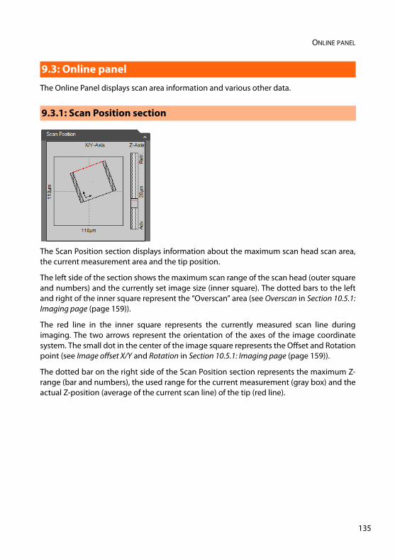
ONLINE PANEL
The Online Panel displays scan area information and various other data.
The Scan Position section displays information about the maximum scan head scan area,the current measurement area and the tip position.
The left side of the section shows the maximum scan range of the scan head (outer squareand numbers) and the currently set image size (inner square). The dotted bars to the leftand right of the inner square represent the “Overscan” area (see Overscan in Section 10.5.1:Imaging page (page 159)).
The red line in the inner square represents the currently measured scan line duringimaging. The two arrows represent the orientation of the axes of the image coordinatesystem. The small dot in the center of the image square represents the Offset and Rotationpoint (see Image offset X/Y and Rotation in Section 10.5.1: Imaging page (page 159)).
The dotted bar on the right side of the Scan Position section represents the maximum Z-range (bar and numbers), the used range for the current measurement (gray box) and theactual Z-position (average of the current scan line) of the tip (red line).
9.3: Online panel
9.3.1: Scan Position section
135
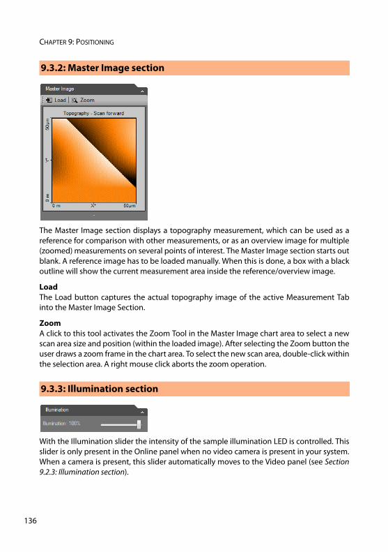
CHAPTER 9: POSITIONING
13
The Master Image section displays a topography measurement, which can be used as areference for comparison with other measurements, or as an overview image for multiple(zoomed) measurements on several points of interest. The Master Image section starts outblank. A reference image has to be loaded manually. When this is done, a box with a blackoutline will show the current measurement area inside the reference/overview image.
LoadThe Load button captures the actual topography image of the active Measurement Tabinto the Master Image Section.
ZoomA click to this tool activates the Zoom Tool in the Master Image chart area to select a newscan area size and position (within the loaded image). After selecting the Zoom button theuser draws a zoom frame in the chart area. To select the new scan area, double-click withinthe selection area. A right mouse click aborts the zoom operation.
With the Illumination slider the intensity of the sample illumination LED is controlled. Thisslider is only present in the Online panel when no video camera is present in your system.When a camera is present, this slider automatically moves to the Video panel (see Section9.2.3: Illumination section).
9.3.2: Master Image section
9.3.3: Illumination section
6
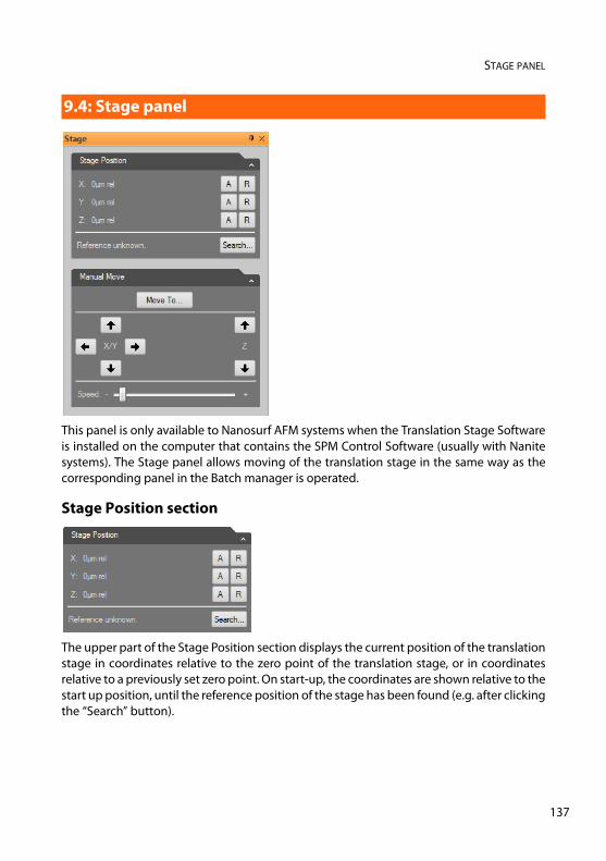
STAGE PANEL
This panel is only available to Nanosurf AFM systems when the Translation Stage Softwareis installed on the computer that contains the SPM Control Software (usually with Nanitesystems). The Stage panel allows moving of the translation stage in the same way as thecorresponding panel in the Batch manager is operated.
Stage Position section
The upper part of the Stage Position section displays the current position of the translationstage in coordinates relative to the zero point of the translation stage, or in coordinatesrelative to a previously set zero point. On start-up, the coordinates are shown relative to thestart up position, until the reference position of the stage has been found (e.g. after clickingthe “Search” button).
9.4: Stage panel
137
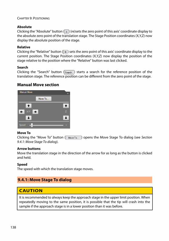
CHAPTER 9: POSITIONING
13
AbsoluteClicking the “Absolute” button ( ) (re)sets the zero point of this axis’ coordinate display tothe absolute zero point of the translation stage. The Stage Position coordinates (X,Y,Z) nowdisplay the absolute position of the stage.
RelativeClicking the “Relative” button ( ) sets the zero point of this axis’ coordinate display to thecurrent position. The Stage Position coordinates (X,Y,Z) now display the position of thestage relative to the position where the “Relative” button was last clicked.
SearchClicking the “Search” button ( ) starts a search for the reference position of thetranslation stage. The reference position can be different from the zero point of the stage.
Manual Move section
Move ToClicking the “Move To” button ( ) opens the Move Stage To dialog (see Section9.4.1: Move Stage To dialog).
Arrow buttonsMove the translation stage in the direction of the arrow for as long as the button is clickedand held.
SpeedThe speed with which the translation stage moves.
9.4.1: Move Stage To dialog
CAUTIONIt is recommended to always keep the approach stage in the upper limit position. Whenrepeatedly moving to the same position, it is possible that the tip will crash into thesample if the approach stage is in a lower position than it was before.
8
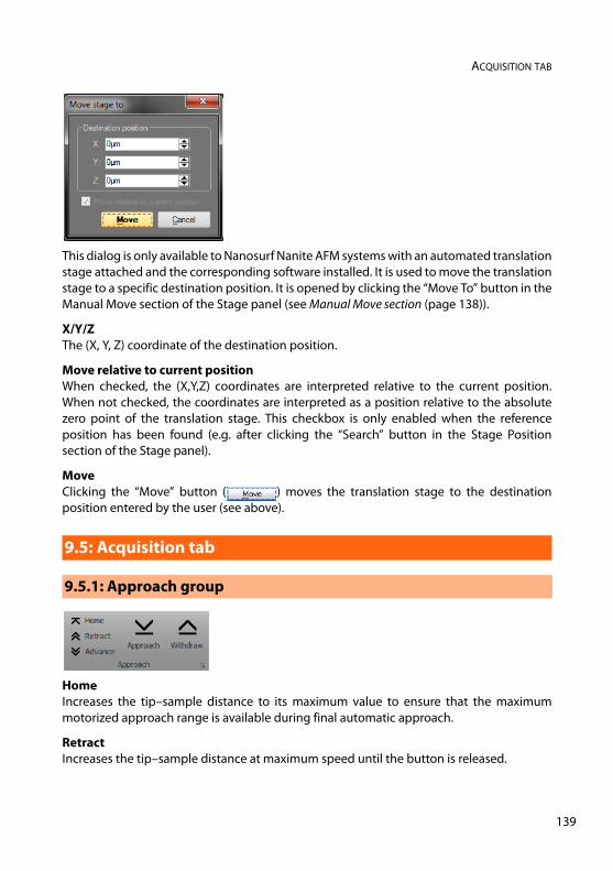
ACQUISITION TAB
This dialog is only available to Nanosurf Nanite AFM systems with an automated translationstage attached and the corresponding software installed. It is used to move the translationstage to a specific destination position. It is opened by clicking the “Move To” button in theManual Move section of the Stage panel (see Manual Move section (page 138)).
X/Y/ZThe (X, Y, Z) coordinate of the destination position.
Move relative to current positionWhen checked, the (X,Y,Z) coordinates are interpreted relative to the current position.When not checked, the coordinates are interpreted as a position relative to the absolutezero point of the translation stage. This checkbox is only enabled when the referenceposition has been found (e.g. after clicking the “Search” button in the Stage Positionsection of the Stage panel).
MoveClicking the “Move” button ( ) moves the translation stage to the destinationposition entered by the user (see above).
HomeIncreases the tip–sample distance to its maximum value to ensure that the maximummotorized approach range is available during final automatic approach.
RetractIncreases the tip–sample distance at maximum speed until the button is released.
9.5: Acquisition tab
9.5.1: Approach group
139
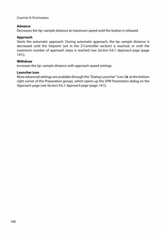
CHAPTER 9: POSITIONING
14
AdvanceDecreases the tip–sample distance at maximum speed until the button is released.
ApproachStarts the automatic approach. During automatic approach, the tip–sample distance isdecreased until the Setpoint (set in the Z-Controller section) is reached, or until themaximum number of approach steps is reached (see Section 9.6.1: Approach page (page141)).
WithdrawIncreases the tip–sample distance with approach speed settings.
Launcher iconMore advanced settings are available through the “Dialog Launcher” icon ( at the bottomright corner of the Preparation group), which opens up the SPM Parameters dialog on theApproach page (see Section 9.6.1: Approach page (page 141)).
0
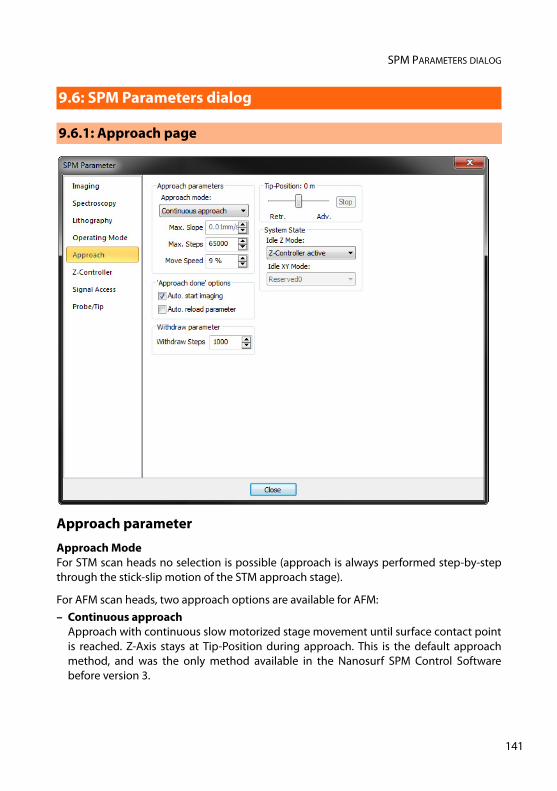
SPM PARAMETERS DIALOG
Approach parameter
Approach ModeFor STM scan heads no selection is possible (approach is always performed step-by-stepthrough the stick-slip motion of the STM approach stage).
For AFM scan heads, two approach options are available for AFM:– Continuous approach
Approach with continuous slow motorized stage movement until surface contact pointis reached. Z-Axis stays at Tip-Position during approach. This is the default approachmethod, and was the only method available in the Nanosurf SPM Control Softwarebefore version 3.
9.6: SPM Parameters dialog
9.6.1: Approach page
141
CHAPTER 9: POSITIONING
14
– Step-By-Step approachApproach is performed by moving the motorized stage quickly over a distance that isless than the scanner’s Z-range. During the movement of the motorized stage, the tip isfully retracted. When the motorized movement is finished, the scanner extends the tipalong the Z-axis to probe for the sample surface. The approach is considered done whenthe Setpoint (defined in the Z-Controller page of the SPM Parameters dialog, or in the Z-Controller section of the Imaging panel of the Imaging window) has been reached. If it isnot reached within the Z-range of the scanner, the tip is again fully retracted and the nextmotorized step is performed. This process of ‘step-and-probe’ is repeated until theSetpoint has been reached (and approach is done). This approach method is consideredto be more ‘gentle’ to tip and sample and should be considered for very sharp tips and/or very soft samples. In general, it does however take more time than Continuousapproach.
Max. SlopeThis parameter defines the speed of extending the z-axis. This parameter is only availablein Step-By-Step approach mode. Slower speeds help to preserve sharp tips.
Max. StepsThis parameter defines the maximal duration of an automatic approach: • In Continuous approach mode it defines the maximum time. • In Step-By-Step approach mode it defines the maximum number of cycles.
Move SpeedThis parameter defines the move speed during automatic approach and withdraw:• In Continuous Approach mode this value should be small. If the approach is too fast, the
tip or the sample surface can be damaged. On the other hand, the motor will not movewhen the move speed is too small.
• In Step-By-Step Approach mode should be around full speed. Lower values help to stopin the z-range of the scanner. On the other hand the approach time increases.
Approach done options
Auto Start imagingWhen selected, the system automatically starts imaging after a successful approach.Scanning automatically stops the approach motor is moved.
Auto Reload parameterWhen selected, the control software reloads the default startup parameter file for eachapproach.
2
ATS STAGE AND TSC 3000 DRIVER CONFIGURATION
Withdraw parameter
Withdraw StepsThe number of steps to use for withdrawing the tip from the sample (see Withdraw (page140)).
Tip-Position
This value determines the Z-Position of the scanner when the approach motor stops. Whenthe Tip-Position is changed when the tip is already approached to the sample, the motorwill move the approach stage so, that the Z-Position of the tip becomes equal to the set Z-Position. When a high resolution scanner is used, the Tip-Position before approach is set toapproximately +500 nm (advanced) by default. This compensates for the residual motionof the approach stage that occurs after the approach motor has stopped.
System State
Idle Z ModeDefines the state of the Z-feedback loop while not measuring. Available options are:– Z-Controller active
Keep the Z-feedback active; the tip is tracking the sample surface.– Retract Tip
This causes the tip to be retracted to the scanner’s upper-most Z-position (farthest awayfrom the sample).
The configuration of the ATS Stage and TSC 3000 Controller is accessed through the TSC3000 driver software. It is only required for AFM systems equipped with such stages andcontrollers (usually Nanite systems).
Starting the TSC 3000 driver
Usually, the TSC 3000 driver start together with the Easyscan 2 control software and will berunning in the background. If this is the case, the tray icon will be visible in theWindows Notification Area (bottom right part of the Windows desktop, also known asSystem Tray).
When the driver is not running:
1 Open the Microsoft Windows “Start” menu.
9.7: ATS Stage and TSC 3000 driver configuration
143
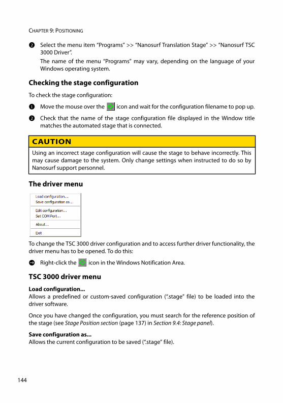
CHAPTER 9: POSITIONING
14
2 Select the menu item “Programs” >> “Nanosurf Translation Stage” >> “Nanosurf TSC3000 Driver”.The name of the menu “Programs” may vary, depending on the language of yourWindows operating system.
Checking the stage configuration
To check the stage configuration:
1 Move the mouse over the icon and wait for the configuration filename to pop up.
2 Check that the name of the stage configuration file displayed in the Window titlematches the automated stage that is connected.
The driver menu
To change the TSC 3000 driver configuration and to access further driver functionality, thedriver menu has to be opened. To do this:
> Right-click the icon in the Windows Notification Area.
TSC 3000 driver menu
Load configuration...Allows a predefined or custom-saved configuration (“.stage” file) to be loaded into thedriver software.
Once you have changed the configuration, you must search for the reference position ofthe stage (see Stage Position section (page 137) in Section 9.4: Stage panel).
Save configuration as...Allows the current configuration to be saved (“.stage” file).
CAUTIONUsing an incorrect stage configuration will cause the stage to behave incorrectly. Thismay cause damage to the system. Only change settings when instructed to do so byNanosurf support personnel.
4
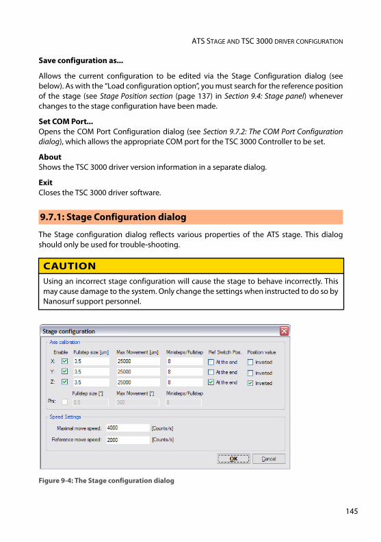
ATS STAGE AND TSC 3000 DRIVER CONFIGURATION
Save configuration as...
Allows the current configuration to be edited via the Stage Configuration dialog (seebelow). As with the “Load configuration option”, you must search for the reference positionof the stage (see Stage Position section (page 137) in Section 9.4: Stage panel) wheneverchanges to the stage configuration have been made.
Set COM Port...Opens the COM Port Configuration dialog (see Section 9.7.2: The COM Port Configurationdialog), which allows the appropriate COM port for the TSC 3000 Controller to be set.
AboutShows the TSC 3000 driver version information in a separate dialog.
ExitCloses the TSC 3000 driver software.
The Stage configuration dialog reflects various properties of the ATS stage. This dialogshould only be used for trouble-shooting.
9.7.1: Stage Configuration dialog
Figure 9-4: The Stage configuration dialog
CAUTIONUsing an incorrect stage configuration will cause the stage to behave incorrectly. Thismay cause damage to the system. Only change the settings when instructed to do so byNanosurf support personnel.
145
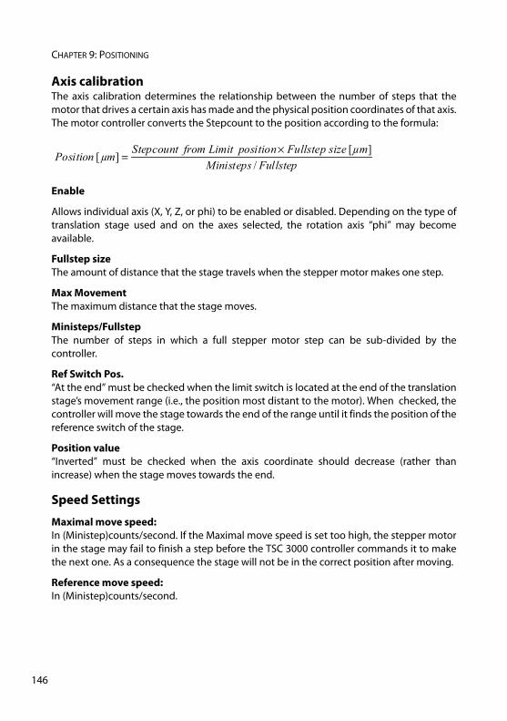
CHAPTER 9: POSITIONING
14
Axis calibrationThe axis calibration determines the relationship between the number of steps that themotor that drives a certain axis has made and the physical position coordinates of that axis.The motor controller converts the Stepcount to the position according to the formula:
Enable
Allows individual axis (X, Y, Z, or phi) to be enabled or disabled. Depending on the type oftranslation stage used and on the axes selected, the rotation axis “phi” may becomeavailable.
Fullstep sizeThe amount of distance that the stage travels when the stepper motor makes one step.
Max MovementThe maximum distance that the stage moves.
Ministeps/FullstepThe number of steps in which a full stepper motor step can be sub-divided by thecontroller.
Ref Switch Pos.“At the end” must be checked when the limit switch is located at the end of the translationstage’s movement range (i.e., the position most distant to the motor). When checked, thecontroller will move the stage towards the end of the range until it finds the position of thereference switch of the stage.
Position value“Inverted” must be checked when the axis coordinate should decrease (rather thanincrease) when the stage moves towards the end.
Speed Settings
Maximal move speed:In (Ministep)counts/second. If the Maximal move speed is set too high, the stepper motorin the stage may fail to finish a step before the TSC 3000 controller commands it to makethe next one. As a consequence the stage will not be in the correct position after moving.
Reference move speed:In (Ministep)counts/second.
FullstepMinistepsµmsizeFullsteppositionLimitfromStepcountµmPosition
/][
][×
=
6
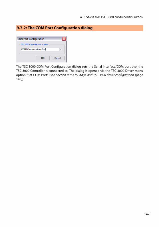
ATS STAGE AND TSC 3000 DRIVER CONFIGURATION
The TSC 3000 COM Port Configuration dialog sets the Serial Interface/COM port that theTSC 3000 Controller is connected to. The dialog is opened via the TSC 3000 Driver menuoption “Set COM Port” (see Section 9.7: ATS Stage and TSC 3000 driver configuration (page143)).
9.7.2: The COM Port Configuration dialog
147

CHAPTER 9: POSITIONING
14
8
CHAPTER 10:
Imaging0
0
CHAPTER 10: IMAGING
15
Imaging measurements of the sample are controlled using the Imaging window. Thischapter describes all elements of the Imaging window in detail. For procedures describinga basic measurements, refer to Chapter 4: A first measurement (page 45). For details on howto use the charts see Section 13.3: Charts (page 209). For advanced imaging settings seeSection 10.5.1: Imaging page.
The Imaging window is contained within the Measurement pane and can be opened byclicking the Imaging tab. The largest part of the Imaging window consists of a number ofcharts that display the data from the ongoing measurement: the Chart area. The imagingwindow can display as many charts as required. Scroll bars will appear automatically assoon as the content is larger than the window can accommodate. By default, two chartsgroups are displayed: 2 color maps of the sample and their corresponding line graphs.Usually, these show Topography on the left and another measurement signal on the right(e.g. Deflection), depending on the current operating mode. For more information onadding and changing charts, which basically works the same for charts in Operatingwindows and in stored measurements documents, see Chapter 13: Working with documents(page 207).
The Parameter area on the left side of the Imaging window, the so-called Imaging panel, isorganized in 3 sections: the “Parameters”, “Z-Controller” and “Mode Properties” section.These sections are an integral part of the Imaging window and represent the mostcommonly used parameters for the currently selected operating mode. Possibleparameters in these sections are described in Section 10.2: Imaging panel. Advancedparameters can be accessed via the “More” button in each section, which will open the SPMParameters dialog on the respective page (see Section 7.9: SPM Parameters dialog (page86)).
At the top, the Imaging window contains a toolbar with commands to control the imagingprocess: the Imaging toolbar. It is described in Section 10.3: The Imaging toolbar.
Apart from the necessary settings, several actions have to be performed before being ableto image a sample. These are accessed via the Acquisition tab of the Ribbon, the elementsof which are described in detail in Section 10.4: Acquisition tab.
Before and during imaging, several panels of the Info pane provide additional informationfor your reference. The relevant panels are explained in Section 9.2: Video panel (page 128)and Section 9.3: Online panel (page 135). A description of the other panels is foundelsewhere in this manual. Please refer to the Chapter 15: Quick reference (page 265) to locatethem.
10.1: Introduction
0
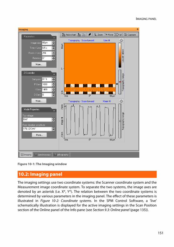
IMAGING PANEL
The imaging settings use two coordinate systems: the Scanner coordinate system and theMeasurement image coordinate system. To separate the two systems, the image axes aredenoted by an asterisk (i.e. X*, Y*). The relation between the two coordinate systems isdetermined by various parameters in the imaging panel. The effect of these parameters isillustrated in Figure 10-2: Coordinate systems. In the SPM Control Software, a ‘live’schematically illustration is displayed for the active imaging settings in the Scan Positionsection of the Online panel of the Info pane (see Section 9.3: Online panel (page 135)).
Figure 10-1: The Imaging window
10.2: Imaging panel
151
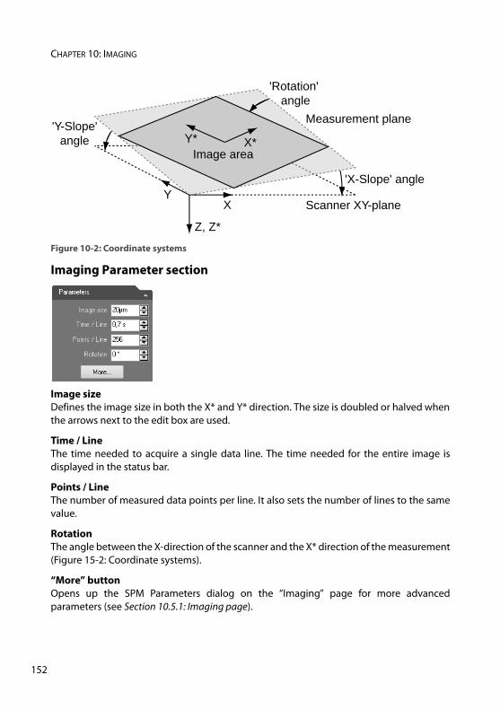
CHAPTER 10: IMAGING
15
Imaging Parameter section
Image size Defines the image size in both the X* and Y* direction. The size is doubled or halved whenthe arrows next to the edit box are used.
Time / Line The time needed to acquire a single data line. The time needed for the entire image isdisplayed in the status bar.
Points / Line The number of measured data points per line. It also sets the number of lines to the samevalue.
Rotation The angle between the X-direction of the scanner and the X* direction of the measurement(Figure 15-2: Coordinate systems).
“More” buttonOpens up the SPM Parameters dialog on the “Imaging” page for more advancedparameters (see Section 10.5.1: Imaging page).
Figure 10-2: Coordinate systems
XY
Z, Z*
Scanner XY-plane
'X-Slope' angle
'Y-Slope' angle
'Rotation' angle
Measurement plane
Image areaX*Y*
2
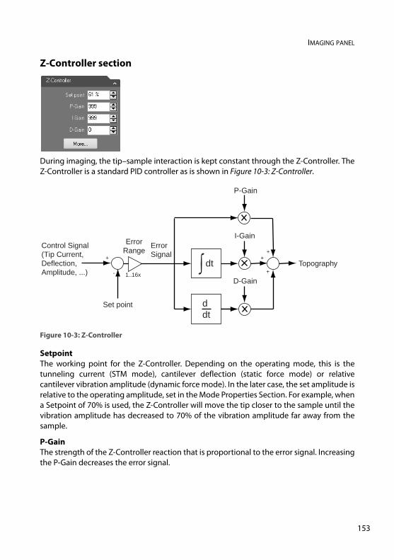
IMAGING PANEL
Z-Controller section
During imaging, the tip–sample interaction is kept constant through the Z-Controller. TheZ-Controller is a standard PID controller as is shown in Figure 10-3: Z-Controller.
SetpointThe working point for the Z-Controller. Depending on the operating mode, this is thetunneling current (STM mode), cantilever deflection (static force mode) or relativecantilever vibration amplitude (dynamic force mode). In the later case, the set amplitude isrelative to the operating amplitude, set in the Mode Properties Section. For example, whena Setpoint of 70% is used, the Z-Controller will move the tip closer to the sample until thevibration amplitude has decreased to 70% of the vibration amplitude far away from thesample.
P-Gain The strength of the Z-Controller reaction that is proportional to the error signal. Increasingthe P-Gain decreases the error signal.
Figure 10-3: Z-Controller
Set point
Topography
ErrorSignal+
-
+Control Signal (Tip Current,Deflection, Amplitude, ...) 1..16x
ErrorRange
P-Gain
D-Gain
I-Gain
dt
d dt
+
+
153
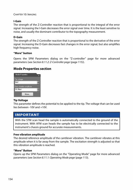
CHAPTER 10: IMAGING
15
I-Gain The strength of the Z-Controller reaction that is proportional to the integral of the errorsignal. Increasing the I-Gain decreases the error signal over time. It is the least sensitive tonoise, and usually the dominant contributor to the topography measurement.
D-Gain The strength of the Z-Controller reaction that is proportional to the derivative of the errorsignal. Increasing the D-Gain decreases fast changes in the error signal, but also amplifieshigh frequency noise.
“More” button
Opens the SPM Parameters dialog on the “Z-controller” page for more advancedparameters (see Section 8.11.2: Z-Controller page (page 115)).
Mode Properties section
Tip Voltage This parameter defines the potential to be applied to the tip. The voltage that can be usedlies between -10V and +10V.
Free vibration amplitudeThe desired reference amplitude of the cantilever vibration. The cantilever vibrates at thisamplitude when it is far away from the sample. The excitation strength is adjusted so thatthis vibration amplitude is reached.
“More” ButtonOpens up the SPM Parameters dialog on the “Operating Mode” page for more advancedparameters (see Section 8.11.1: Operating Mode page (page 113).
IMPORTANTWith the STM scan head the sample is automatically connected to the ground of theinstrument. With AFM scan heads the sample has to be electrically connected to theinstrument’s chassis ground for accurate measurements.
4
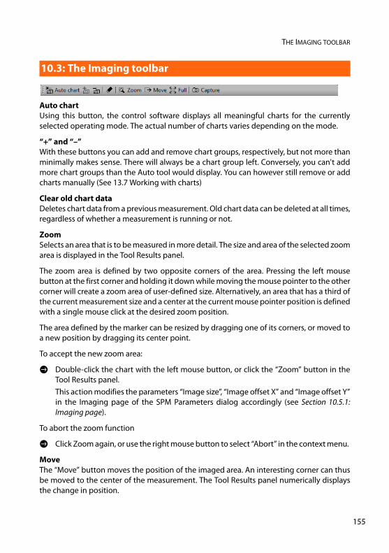
THE IMAGING TOOLBAR
Auto chartUsing this button, the control software displays all meaningful charts for the currentlyselected operating mode. The actual number of charts varies depending on the mode.
“+” and “–”With these buttons you can add and remove chart groups, respectively, but not more thanminimally makes sense. There will always be a chart group left. Conversely, you can't addmore chart groups than the Auto tool would display. You can however still remove or addcharts manually (See 13.7 Working with charts)
Clear old chart dataDeletes chart data from a previous measurement. Old chart data can be deleted at all times,regardless of whether a measurement is running or not.
Zoom Selects an area that is to be measured in more detail. The size and area of the selected zoomarea is displayed in the Tool Results panel.
The zoom area is defined by two opposite corners of the area. Pressing the left mousebutton at the first corner and holding it down while moving the mouse pointer to the othercorner will create a zoom area of user-defined size. Alternatively, an area that has a third ofthe current measurement size and a center at the current mouse pointer position is definedwith a single mouse click at the desired zoom position.
The area defined by the marker can be resized by dragging one of its corners, or moved toa new position by dragging its center point.
To accept the new zoom area:
> Double-click the chart with the left mouse button, or click the “Zoom” button in theTool Results panel. This action modifies the parameters “Image size”, “Image offset X” and “Image offset Y”in the Imaging page of the SPM Parameters dialog accordingly (see Section 10.5.1:Imaging page).
To abort the zoom function
> Click Zoom again, or use the right mouse button to select “Abort” in the context menu.
MoveThe “Move” button moves the position of the imaged area. An interesting corner can thusbe moved to the center of the measurement. The Tool Results panel numerically displaysthe change in position.
10.3: The Imaging toolbar
155
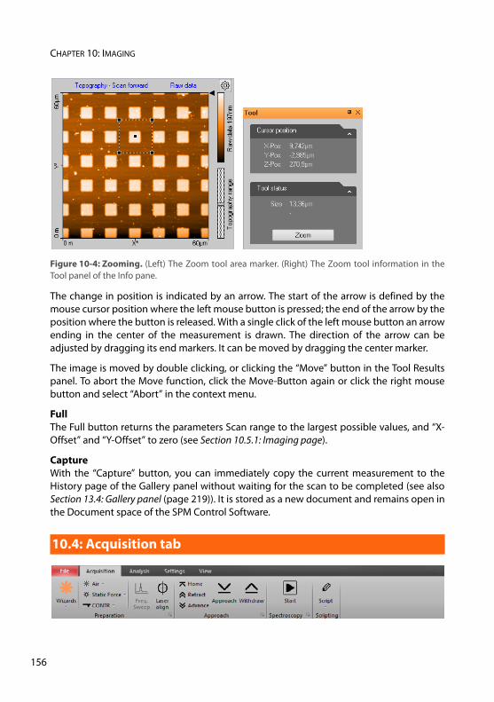
CHAPTER 10: IMAGING
15
The change in position is indicated by an arrow. The start of the arrow is defined by themouse cursor position where the left mouse button is pressed; the end of the arrow by theposition where the button is released. With a single click of the left mouse button an arrowending in the center of the measurement is drawn. The direction of the arrow can beadjusted by dragging its end markers. It can be moved by dragging the center marker.
The image is moved by double clicking, or clicking the “Move” button in the Tool Resultspanel. To abort the Move function, click the Move-Button again or click the right mousebutton and select “Abort” in the context menu.
FullThe Full button returns the parameters Scan range to the largest possible values, and “X-Offset” and “Y-Offset” to zero (see Section 10.5.1: Imaging page).
CaptureWith the “Capture” button, you can immediately copy the current measurement to theHistory page of the Gallery panel without waiting for the scan to be completed (see alsoSection 13.4: Gallery panel (page 219)). It is stored as a new document and remains open inthe Document space of the SPM Control Software.
Figure 10-4: Zooming. (Left) The Zoom tool area marker. (Right) The Zoom tool information in theTool panel of the Info pane.
10.4: Acquisition tab
6
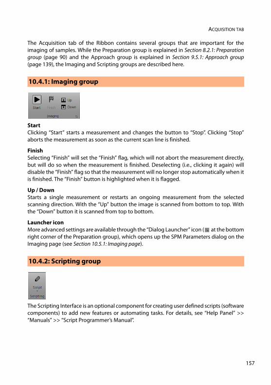
ACQUISITION TAB
The Acquisition tab of the Ribbon contains several groups that are important for theimaging of samples. While the Preparation group is explained in Section 8.2.1: Preparationgroup (page 90) and the Approach group is explained in Section 9.5.1: Approach group(page 139), the Imaging and Scripting groups are described here.
StartClicking “Start” starts a measurement and changes the button to “Stop”. Clicking “Stop”aborts the measurement as soon as the current scan line is finished.
Finish Selecting “Finish” will set the “Finish” flag, which will not abort the measurement directly,but will do so when the measurement is finished. Deselecting (i.e., clicking it again) willdisable the “Finish” flag so that the measurement will no longer stop automatically when itis finished. The “Finish” button is highlighted when it is flagged.
Up / DownStarts a single measurement or restarts an ongoing measurement from the selectedscanning direction. With the “Up” button the image is scanned from bottom to top. Withthe “Down” button it is scanned from top to bottom.
Launcher iconMore advanced settings are available through the “Dialog Launcher” icon ( at the bottomright corner of the Preparation group), which opens up the SPM Parameters dialog on theImaging page (see Section 10.5.1: Imaging page).
The Scripting Interface is an optional component for creating user defined scripts (softwarecomponents) to add new features or automating tasks. For details, see “Help Panel” >>“Manuals” >> “Script Programmer’s Manual”.
10.4.1: Imaging group
10.4.2: Scripting group
157
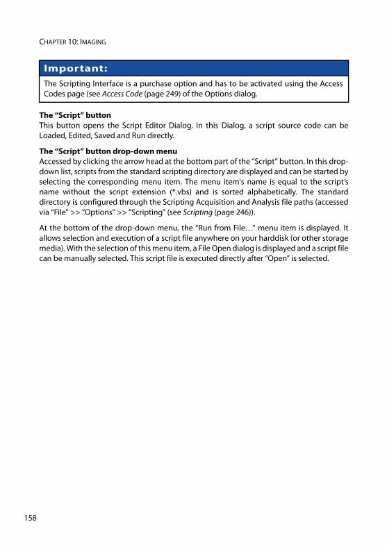
CHAPTER 10: IMAGING
15
The “Script” button This button opens the Script Editor Dialog. In this Dialog, a script source code can beLoaded, Edited, Saved and Run directly.
The “Script” button drop-down menuAccessed by clicking the arrow head at the bottom part of the “Script” button. In this drop-down list, scripts from the standard scripting directory are displayed and can be started byselecting the corresponding menu item. The menu item's name is equal to the script’sname without the script extension (*.vbs) and is sorted alphabetically. The standarddirectory is configured through the Scripting Acquisition and Analysis file paths (accessedvia “File” >> “Options” >> “Scripting” (see Scripting (page 246)).
At the bottom of the drop-down menu, the “Run from File…” menu item is displayed. Itallows selection and execution of a script file anywhere on your harddisk (or other storagemedia). With the selection of this menu item, a File Open dialog is displayed and a script filecan be manually selected. This script file is executed directly after “Open” is selected.
Important:The Scripting Interface is a purchase option and has to be activated using the AccessCodes page (see Access Code (page 249) of the Options dialog.
8
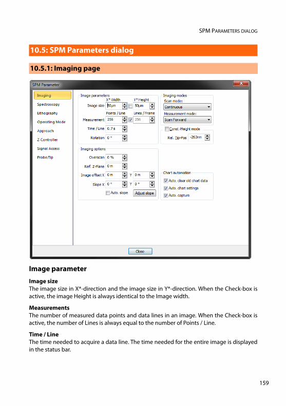
SPM PARAMETERS DIALOG
Image parameter
Image sizeThe image size in X*-direction and the image size in Y*-direction. When the Check-box isactive, the image Height is always identical to the Image width.
MeasurementsThe number of measured data points and data lines in an image. When the Check-box isactive, the number of Lines is always equal to the number of Points / Line.
Time / Line The time needed to acquire a data line. The time needed for the entire image is displayedin the status bar.
10.5: SPM Parameters dialog
10.5.1: Imaging page
159
CHAPTER 10: IMAGING
16
Rotation The angle between the X-direction of the scanner and the X* direction of the measurement(Figure 15-2: Coordinate systems).
Imaging options
Overscan The “Overscan” determines how much the effective scan range is increased relative to theimage width. This will eliminate edge effects caused by the reversal of the scanning motionby not recording or displaying them in the measurement image. Disadvantages of usingOverscan are that the maximum scan range is reduced, the tip moves slightly faster overthe sample with the same “Time/Line” setting, and the tip may hit large features outside themeasured image.
Ref. Z-Plane The height of the reference plane. This height reference is used when the Z-Controlleroutput is cleared, and when the Z-position is not modulated relative to the current surfaceposition during spectroscopy measurements.
The reference plane for the image can be aligned to the surface of the sample using theslope parameters (see Figure 5-2: Sample and measurement orientation before slopeadjustment (page 64) or Figure 10-2: Coordinate systems (page 152)).
Image offset X/YThe center position of the measured area.
Slope XA positive value rotates the image plane around the Y-axis counterclockwise.
Slope YA positive value rotates the image plane around the X-axis counterclockwise.
The center position of the measured area can be changed by typing its position as well asby using the Move tool in the Imaging toolbar. The zero position corresponds to the centerposition of the scanner.
Adjust slopeThe “Adjust slope” button will cause the control software to set appropriate values for X-and Y-slope by performing two single line scans (one in X- and one in Y-direction) anddetermining the respective slopes via line fitting, thus electronically compensating forthese measurement plane slopes (see Section 5.2: Adjusting the measurement plane (page63) for details).
Auto slope Automatically performs the same action as the “Adjust slope” button does. It adjusts theslopes with each new “Start” of imaging.
0
SPM PARAMETERS DIALOG
Imaging modes
Scan mode This parameter defines how the images are acquired and displayed: – Continuous
The acquisition direction is reversed after each scan: from bottom to top and vice versa.– Cont.Up
The acquisition direction is always from bottom to top.– Cont.Down
The acquisition direction is always from top to bottom.
Measurement modeThis parameter defines how each imaging line is acquired and stored: – Forward
During forward scan only (left to right in the image). – Backward
During backward scan only (right to left in the image). – Forw.&Backw.
During both forward and backward scan.
Const. Height mode
When the Constant Height imaging mode is enabled, the Z-Controller is turned off duringthe scan (as a consequence, the Probe Status light will blink green). Instead, the scannerscans along a straight line, that should be parallel to the surface. The slope of the line isdefined by the X- and Y-Slope parameters. These parameters should be set as described inSection 5.2: Adjusting the measurement plane (page 63). The height of the line is determinedat the start of each scan line: First the Z-Controller is turned on. Once the tip position isstable, the Z-Controller is turned off and the tip is moved away from the sample by thedistance set by the parameter Rel. Tip-Pos.
The Constant Height Imaging mode is mainly useful for EFM and MFM measurements. Formore information on how to do Magnetic Force Microscopy, refer to technical note“TN00031 — Operating Nanosurf AFMs in MFM mode” which can be found in the“Technote” section of the Help panel.
Rel. Tip-Pos This parameter defines the distance by which the Tip is moved towards the sample fromthe position that corresponds to the Setpoint. A negative setting will move the tip awayfrom the sample.
161
CHAPTER 10: IMAGING
16
Chart automation
Auto clear old chart dataAutomatically clear the chart data from a measurement when a measurement is restarted(either when a scan is restarted manually, or when a previous scan has finished andmeasurement recommences as determined by the scan mode (see Scan mode (page 161).
Auto chart settingsIf checked, the chart arrangement is automatically updated (see also Auto chart (page 155)).
Auto CaptureIf checked, all measurements are automatically stored in the history Gallery. If unchecked,you have to click the “Capture” button in the Imaging tool bar to manually save yourmeasurement data.
2

CHAPTER 11:
Spectroscopy0
0
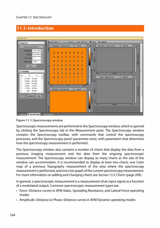
CHAPTER 11: SPECTROSCOPY
16
Spectroscopic measurements are performed in the Spectroscopy window, which is openedby clicking the Spectroscopy tab in the Measurement pane. The Spectroscopy windowcontains the Spectroscopy toolbar, with commands that control the spectroscopyprocesses, and the Spectroscopy panel (parameter area), with parameters that determinehow the spectroscopy measurement is performed.
The Spectroscopy window also contains a number of charts that display the data from aprevious imaging measurement and the data from the ongoing spectroscopicmeasurement. The Spectroscopy window can display as many charts as the size of thewindow can accommodate. It is recommended to display at least two charts, one Colormap of a previous Topography measurement of the area where the spectroscopymeasurement is performed, and one Line graph of the current spectroscopy measurement.For more information on adding and changing charts see Section 13.3: Charts (page 209).
In general, a spectroscopic measurement is a measurement of an input signal as a functionof a modulated output. Common spectroscopic measurement types are:• Force–Distance curves in AFM Static, Spreading Resistance, and Lateral Force operating
modes• Amplitude–Distance or Phase–Distance curves in AFM Dynamic operating modes
Figure 11-1: Spectroscopy window
11.1: Introduction
4
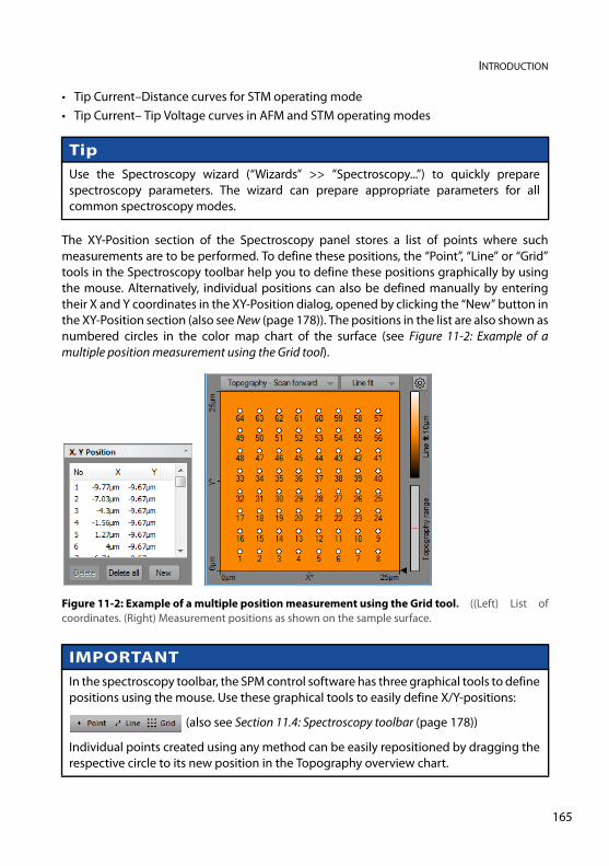
INTRODUCTION
• Tip Current–Distance curves for STM operating mode• Tip Current– Tip Voltage curves in AFM and STM operating modes
The XY-Position section of the Spectroscopy panel stores a list of points where suchmeasurements are to be performed. To define these positions, the “Point”, “Line” or “Grid”tools in the Spectroscopy toolbar help you to define these positions graphically by usingthe mouse. Alternatively, individual positions can also be defined manually by enteringtheir X and Y coordinates in the XY-Position dialog, opened by clicking the “New” button inthe XY-Position section (also see New (page 178)). The positions in the list are also shown asnumbered circles in the color map chart of the surface (see Figure 11-2: Example of amultiple position measurement using the Grid tool).
TipUse the Spectroscopy wizard (“Wizards” >> ”Spectroscopy...”) to quickly preparespectroscopy parameters. The wizard can prepare appropriate parameters for allcommon spectroscopy modes.
Figure 11-2: Example of a multiple position measurement using the Grid tool. ((Left) List ofcoordinates. (Right) Measurement positions as shown on the sample surface.
IMPORTANTIn the spectroscopy toolbar, the SPM control software has three graphical tools to definepositions using the mouse. Use these graphical tools to easily define X/Y-positions:
(also see Section 11.4: Spectroscopy toolbar (page 178))
Individual points created using any method can be easily repositioned by dragging therespective circle to its new position in the Topography overview chart.
165
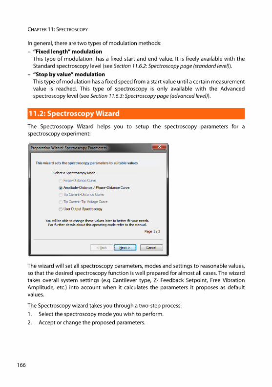
CHAPTER 11: SPECTROSCOPY
16
In general, there are two types of modulation methods:– “Fixed length” modulation
This type of modulation has a fixed start and end value. It is freely available with theStandard spectroscopy level (see Section 11.6.2: Spectroscopy page (standard level)).
– “Stop by value” modulationThis type of modulation has a fixed speed from a start value until a certain measurementvalue is reached. This type of spectroscopy is only available with the Advancedspectroscopy level (see Section 11.6.3: Spectroscopy page (advanced level)).
The Spectroscopy Wizard helps you to setup the spectroscopy parameters for aspectroscopy experiment:
The wizard will set all spectroscopy parameters, modes and settings to reasonable values,so that the desired spectroscopy function is well prepared for almost all cases. The wizardtakes overall system settings (e.g Cantilever type, Z- Feedback Setpoint, Free VibrationAmplitude, etc.) into account when it calculates the parameters it proposes as defaultvalues.
The Spectroscopy wizard takes you through a two-step process:1. Select the spectroscopy mode you wish to perform. 2. Accept or change the proposed parameters.
11.2: Spectroscopy Wizard
6
SPECTROSCOPY WIZARD
After clicking the “Finish” button, the Wizard sets all spectroscopy parameters. These canbe viewed in the Spectroscopy page of the SPM Parameters dialog (see Section 11.6.1:Spectroscopy page) and may be adjusted at any time to better fit your needs.
If already approached to the surface, you are ready to start the Spectroscopy by clicking the“Start” button in the Spectroscopy group of the Acquisition ribbon (see Section 11.5.1:Spectroscopy group). If no X/Y-Position is defined, spectroscopy will be performed in thecenter of the image, respecting the selected XY-offset in the imaging parameters.
6.1.1
The Force–Distance curve is a spectroscopy mode where the cantilever is moved while thedeflection signal is measured. With Force–Distance spectroscopy, the typical snap-in andrelease effect of the tip–sample interaction can be measured. Additionally, the cantileverspring constant and the system’s deflection sensitivity can be precisely calibrated (seeSection 14.8.2: Probe/Tip page (page 262)).
A “fixed length” modulation can be safely performed with the Standard Spectroscopy levelwhen the tip starts at the surface (and the Z-position of the surface is therefore alreadyknown) and is subsequently moved away to a retracted position and then back again.
A “stop by value” modulation can only be performed with the Advanced Spectroscopy levelsince only there the it is possible to enter an appropriate stop value. Here it is also possibleto start from a retracted position and then move towards the surface until a given Stopcriterion is reached and to retract again afterwards.
A “fixed length” Force–Distance spectroscopy experiment is typically divided into 4 distinctphases (see Figure 11-3, Left):1. Tip is approached (i.e. in contact with the surface).2. Move the tip to a defined position (Range) above the surface while measuring the
deflection signal (and any other input signals that the current measurement modemay allow). This is called the “Forward Modulation phase”.
IMPORTANT• A disabled spectroscopy mode means that this mode is not available for the currently
selected operating mode. “Amplitude–Distance curve”, for example, is only possible in“Dynamic Force” or “Phase Contrast” operating modes and not in “Static Force”operating mode.
• A disabled parameter means that it is only available if the Advanced SpectroscopyLevel is activated by a correct Access code (see Access Code (page 249)).
11.2.1: Force–Distance
167
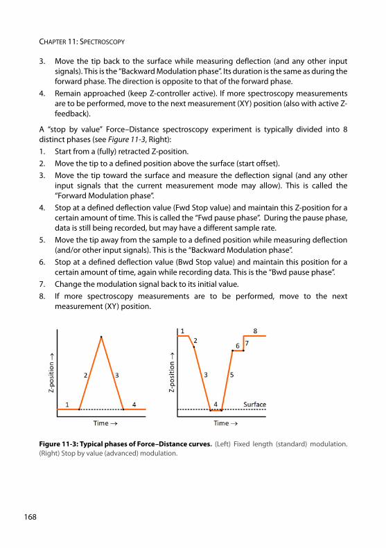
CHAPTER 11: SPECTROSCOPY
16
3. Move the tip back to the surface while measuring deflection (and any other inputsignals). This is the “Backward Modulation phase”. Its duration is the same as during theforward phase. The direction is opposite to that of the forward phase.
4. Remain approached (keep Z-controller active). If more spectroscopy measurementsare to be performed, move to the next measurement (XY) position (also with active Z-feedback).
A “stop by value” Force–Distance spectroscopy experiment is typically divided into 8distinct phases (see Figure 11-3, Right):1. Start from a (fully) retracted Z-position.2. Move the tip to a defined position above the surface (start offset).3. Move the tip toward the surface and measure the deflection signal (and any other
input signals that the current measurement mode may allow). This is called the“Forward Modulation phase”.
4. Stop at a defined deflection value (Fwd Stop value) and maintain this Z-position for acertain amount of time. This is called the “Fwd pause phase”. During the pause phase,data is still being recorded, but may have a different sample rate.
5. Move the tip away from the sample to a defined position while measuring deflection(and/or other input signals). This is the “Backward Modulation phase”.
6. Stop at a defined deflection value (Bwd Stop value) and maintain this position for acertain amount of time, again while recording data. This is the “Bwd pause phase”.
7. Change the modulation signal back to its initial value. 8. If more spectroscopy measurements are to be performed, move to the next
measurement (XY) position.
Figure 11-3: Typical phases of Force–Distance curves. (Left) Fixed length (standard) modulation.(Right) Stop by value (advanced) modulation.
8
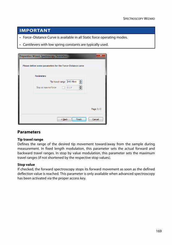
SPECTROSCOPY WIZARD
Parameters
Tip travel rangeDefines the range of the desired tip movement toward/away from the sample duringmeasurement. In fixed length modulation, this parameter sets the actual forward andbackward travel ranges. In stop by value modulation, this parameter sets the maximumtravel ranges (if not shortened by the respective stop values).
Stop valueIf checked, the forward spectroscopy stops its forward movement as soon as the defineddeflection value is reached. This parameter is only available when advanced spectroscopyhas been activated via the proper access key.
IMPORTANT• Force–Distance Curve is available in all Static force operating modes.
• Cantilevers with low spring constants are typically used.
169
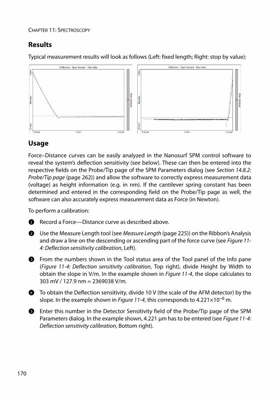
CHAPTER 11: SPECTROSCOPY
17
Results
Typical measurement results will look as follows (Left: fixed length; Right: stop by value):
Usage
Force–Distance curves can be easily analyzed in the Nanosurf SPM control software toreveal the system’s deflection sensitivity (see below). These can then be entered into therespective fields on the Probe/Tip page of the SPM Parameters dialog (see Section 14.8.2:Probe/Tip page (page 262)) and allow the software to correctly express measurement data(voltage) as height information (e.g. in nm). If the cantilever spring constant has beendetermined and entered in the corresponding field on the Probe/Tip page as well, thesoftware can also accurately express measurement data as Force (in Newton).
To perform a calibration:
1 Record a Force—Distance curve as described above.
2 Use the Measure Length tool (see Measure Length (page 225)) on the Ribbon’s Analysisand draw a line on the descending or ascending part of the force curve (see Figure 11-4: Deflection sensitivity calibration, Left).
3 From the numbers shown in the Tool status area of the Tool panel of the Info pane(Figure 11-4: Deflection sensitivity calibration, Top right), divide Height by Width toobtain the slope in V/m. In the example shown in Figure 11-4, the slope calculates to303 mV / 127.9 nm = 2369038 V/m.
4 To obtain the Deflection sensitivity, divide 10 V (the scale of the AFM detector) by theslope. In the example shown in Figure 11-4, this corresponds to 4.221×10⁻⁶ m.
5 Enter this number in the Detector Sensitivity field of the Probe/Tip page of the SPMParameters dialog. In the example shown, 4.221 μm has to be entered (see Figure 11-4:Deflection sensitivity calibration, Bottom right).
0
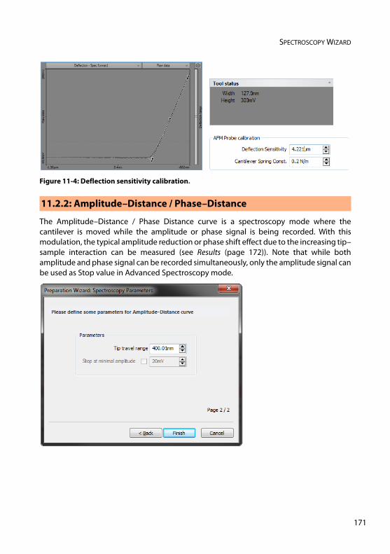
SPECTROSCOPY WIZARD
6.1.2
The Amplitude–Distance / Phase Distance curve is a spectroscopy mode where thecantilever is moved while the amplitude or phase signal is being recorded. With thismodulation, the typical amplitude reduction or phase shift effect due to the increasing tip–sample interaction can be measured (see Results (page 172)). Note that while bothamplitude and phase signal can be recorded simultaneously, only the amplitude signal canbe used as Stop value in Advanced Spectroscopy mode.
Figure 11-4: Deflection sensitivity calibration.
11.2.2: Amplitude–Distance / Phase–Distance
171
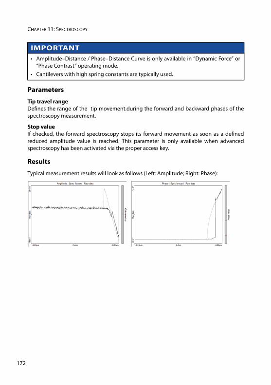
CHAPTER 11: SPECTROSCOPY
17
Parameters
Tip travel rangeDefines the range of the tip movement.during the forward and backward phases of thespectroscopy measurement.
Stop valueIf checked, the forward spectroscopy stops its forward movement as soon as a definedreduced amplitude value is reached. This parameter is only available when advancedspectroscopy has been activated via the proper access key.
Results
Typical measurement results will look as follows (Left: Amplitude; Right: Phase):
IMPORTANT• Amplitude–Distance / Phase–Distance Curve is only available in “Dynamic Force” or
“Phase Contrast” operating mode. • Cantilevers with high spring constants are typically used.
2
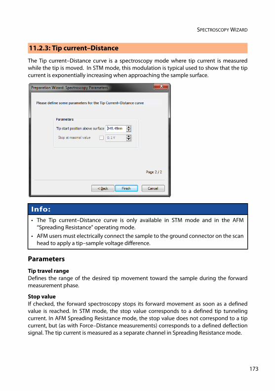
SPECTROSCOPY WIZARD
6.1.3
The Tip current–Distance curve is a spectroscopy mode where tip current is measuredwhile the tip is moved. In STM mode, this modulation is typical used to show that the tipcurrent is exponentially increasing when approaching the sample surface.
Parameters
Tip travel rangeDefines the range of the desired tip movement toward the sample during the forwardmeasurement phase.
Stop valueIf checked, the forward spectroscopy stops its forward movement as soon as a definedvalue is reached. In STM mode, the stop value corresponds to a defined tip tunnelingcurrent. In AFM Spreading Resistance mode, the stop value does not correspond to a tipcurrent, but (as with Force–Distance measurements) corresponds to a defined deflectionsignal. The tip current is measured as a separate channel in Spreading Resistance mode.
11.2.3: Tip current–Distance
Info:• The Tip current–Distance curve is only available in STM mode and in the AFM
“Spreading Resistance” operating mode.• AFM users must electrically connect the sample to the ground connector on the scan
head to apply a tip–sample voltage difference.
173
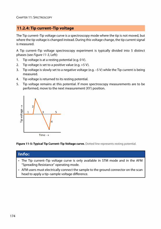
CHAPTER 11: SPECTROSCOPY
17
6.1.4
The Tip current–Tip voltage curve is a spectroscopy mode where the tip is not moved, butwhere the tip voltage is changed instead. During this voltage change, the tip current signalis measured.
A Tip current–Tip voltage spectroscopy experiment is typically divided into 5 distinctphases (see Figure 11-3, Left):1. Tip voltage is at a resting potential (e.g. 0 V).2. Tip voltage is set to a positive value (e.g. +5 V).3. Tip voltage is slowly set to a negative voltage (e.g. –5 V) while the Tip current is being
measured.4. Tip voltage is returned to its resting potential.5. Tip voltage remains at this potential. If more spectroscopy measurements are to be
performed, move to the next measurement (XY) position.
11.2.4: Tip current–Tip voltage
Figure 11-5: Typical Tip Current–Tip Voltage curve. Dotted line represents resting potential.
Info:• The Tip current–Tip voltage curve is only available in STM mode and in the AFM
“Spreading Resistance” operating mode.• AFM users must electrically connect the sample to the ground connector on the scan
head to apply a tip–sample voltage difference.
4
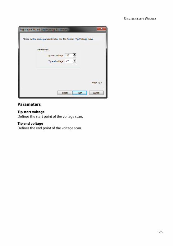
SPECTROSCOPY WIZARD
Parameters
Tip start voltageDefines the start point of the voltage scan.
Tip end voltageDefines the end point of the voltage scan.
175
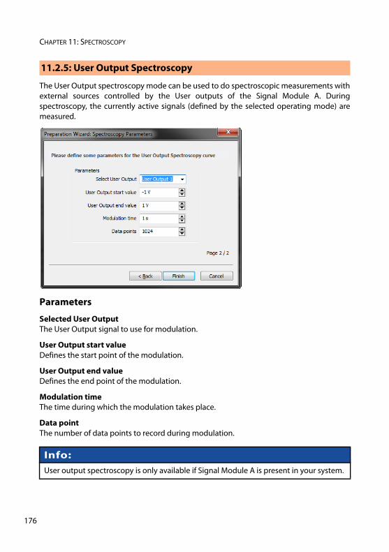
CHAPTER 11: SPECTROSCOPY
17
6.1.5
The User Output spectroscopy mode can be used to do spectroscopic measurements withexternal sources controlled by the User outputs of the Signal Module A. Duringspectroscopy, the currently active signals (defined by the selected operating mode) aremeasured.
Parameters
Selected User OutputThe User Output signal to use for modulation.
User Output start valueDefines the start point of the modulation.
User Output end valueDefines the end point of the modulation.
Modulation timeThe time during which the modulation takes place.
Data pointThe number of data points to record during modulation.
11.2.5: User Output Spectroscopy
Info:User output spectroscopy is only available if Signal Module A is present in your system.
6
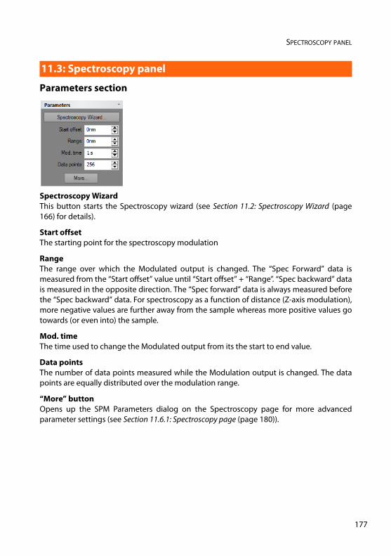
SPECTROSCOPY PANEL
Parameters section
Spectroscopy WizardThis button starts the Spectroscopy wizard (see Section 11.2: Spectroscopy Wizard (page166) for details).
Start offsetThe starting point for the spectroscopy modulation
RangeThe range over which the Modulated output is changed. The “Spec Forward” data ismeasured from the “Start offset” value until “Start offset” + “Range”. “Spec backward” datais measured in the opposite direction. The “Spec forward” data is always measured beforethe “Spec backward” data. For spectroscopy as a function of distance (Z-axis modulation),more negative values are further away from the sample whereas more positive values gotowards (or even into) the sample.
Mod. time The time used to change the Modulated output from its the start to end value.
Data points The number of data points measured while the Modulation output is changed. The datapoints are equally distributed over the modulation range.
“More” buttonOpens up the SPM Parameters dialog on the Spectroscopy page for more advancedparameter settings (see Section 11.6.1: Spectroscopy page (page 180)).
11.3: Spectroscopy panel
177
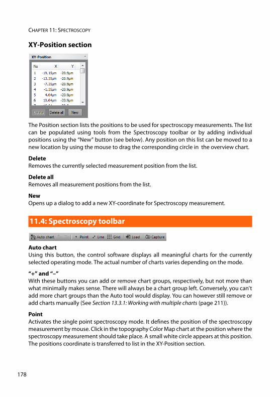
CHAPTER 11: SPECTROSCOPY
17
XY-Position section
The Position section lists the positions to be used for spectroscopy measurements. The listcan be populated using tools from the Spectroscopy toolbar or by adding individualpositions using the “New” button (see below). Any position on this list can be moved to anew location by using the mouse to drag the corresponding circle in the overview chart.
DeleteRemoves the currently selected measurement position from the list.
Delete allRemoves all measurement positions from the list.
NewOpens up a dialog to add a new XY-coordinate for Spectroscopy measurement.
Auto chartUsing this button, the control software displays all meaningful charts for the currentlyselected operating mode. The actual number of charts varies depending on the mode.
“+” and “–”With these buttons you can add or remove chart groups, respectively, but not more thanwhat minimally makes sense. There will always be a chart group left. Conversely, you can'tadd more chart groups than the Auto tool would display. You can however still remove oradd charts manually (See Section 13.3.1: Working with multiple charts (page 211)).
PointActivates the single point spectroscopy mode. It defines the position of the spectroscopymeasurement by mouse. Click in the topography Color Map chart at the position where thespectroscopy measurement should take place. A small white circle appears at this position.The positions coordinate is transferred to list in the XY-Position section.
11.4: Spectroscopy toolbar
8
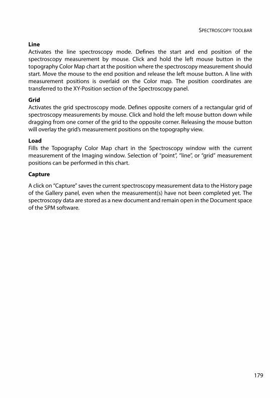
SPECTROSCOPY TOOLBAR
LineActivates the line spectroscopy mode. Defines the start and end position of thespectroscopy measurement by mouse. Click and hold the left mouse button in thetopography Color Map chart at the position where the spectroscopy measurement shouldstart. Move the mouse to the end position and release the left mouse button. A line withmeasurement positions is overlaid on the Color map. The position coordinates aretransferred to the XY-Position section of the Spectroscopy panel.
GridActivates the grid spectroscopy mode. Defines opposite corners of a rectangular grid ofspectroscopy measurements by mouse. Click and hold the left mouse button down whiledragging from one corner of the grid to the opposite corner. Releasing the mouse buttonwill overlay the grid’s measurement positions on the topography view.
LoadFills the Topography Color Map chart in the Spectroscopy window with the currentmeasurement of the Imaging window. Selection of “point”, “line”, or “grid” measurementpositions can be performed in this chart.
Capture
A click on “Capture” saves the current spectroscopy measurement data to the History pageof the Gallery panel, even when the measurement(s) have not been completed yet. Thespectroscopy data are stored as a new document and remain open in the Document spaceof the SPM software.
179
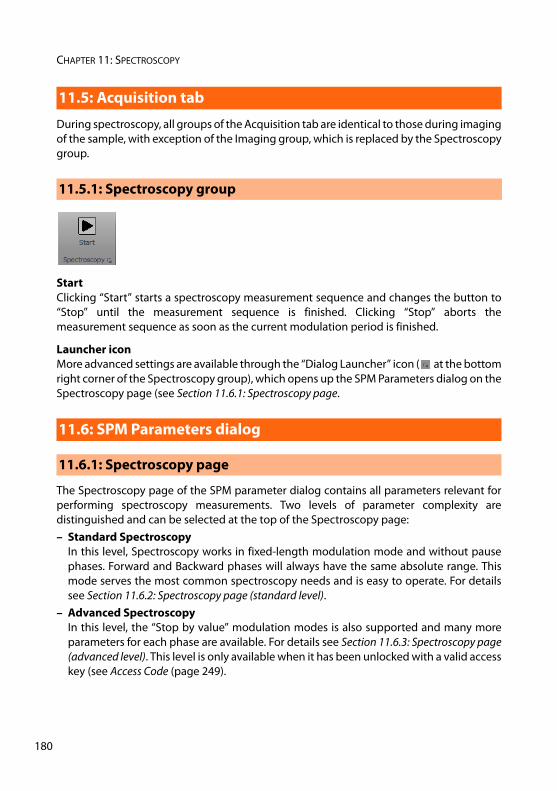
CHAPTER 11: SPECTROSCOPY
18
During spectroscopy, all groups of the Acquisition tab are identical to those during imagingof the sample, with exception of the Imaging group, which is replaced by the Spectroscopygroup.
StartClicking “Start” starts a spectroscopy measurement sequence and changes the button to“Stop” until the measurement sequence is finished. Clicking “Stop” aborts themeasurement sequence as soon as the current modulation period is finished.
Launcher iconMore advanced settings are available through the “Dialog Launcher” icon ( at the bottomright corner of the Spectroscopy group), which opens up the SPM Parameters dialog on theSpectroscopy page (see Section 11.6.1: Spectroscopy page.
The Spectroscopy page of the SPM parameter dialog contains all parameters relevant forperforming spectroscopy measurements. Two levels of parameter complexity aredistinguished and can be selected at the top of the Spectroscopy page:– Standard Spectroscopy
In this level, Spectroscopy works in fixed-length modulation mode and without pausephases. Forward and Backward phases will always have the same absolute range. Thismode serves the most common spectroscopy needs and is easy to operate. For detailssee Section 11.6.2: Spectroscopy page (standard level).
– Advanced SpectroscopyIn this level, the “Stop by value” modulation modes is also supported and many moreparameters for each phase are available. For details see Section 11.6.3: Spectroscopy page(advanced level). This level is only available when it has been unlocked with a valid accesskey (see Access Code (page 249).
11.5: Acquisition tab
11.5.1: Spectroscopy group
11.6: SPM Parameters dialog
11.6.1: Spectroscopy page
0
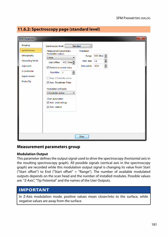
SPM PARAMETERS DIALOG
Measurement parameters group
Modulation OutputThis parameter defines the output signal used to drive the spectroscopy (horizontal axis inthe resulting spectroscopy graph). All possible signals (vertical axis in the spectroscopygraph) are recorded while this modulation output signal is changing its value from Start(“Start offset”) to End (“Start offset” + “Range”). The number of available modulatedoutputs depends on the scan head and the number of installed modules. Possible valuesare: “Z-Axis”, “Tip Potential” and the names of the User Outputs.
11.6.2: Spectroscopy page (standard level)
IMPORTANTIn Z-Axis modulation mode, positive values mean closer/into to the surface, whilenegative values are away from the surface.
181
CHAPTER 11: SPECTROSCOPY
18
Start OffsetDefines the absolute or relative start value of the modulated output signal during a newmodulation.
Relative to current valueIf checked, the start offset value is used as a value relative to the current value. If uncheckedthe Start Offset is used as an absolute value for the start of a new modulation. In case of Z-Axis modulation, the last known surface position is used as reference point. This means thatif the tip was at some point retracted after approach, it still uses the Z-height at whichcontact was established.
RepetitionThis value defines the number of times a modulation measurement is repeated at each XY-Position. Each measurement is stored individually.
Keep Z Controller activeWhen checked, the Z-Controller will continue to change the Z-position to keep the tip–sample interaction constant. This option is not available when the Modulated output is setto Z-Axis. This setting can for example be used to measure Tip current as a function ofapplied voltage while keeping the tip–sample force constant. If unchecked, the Z-Axis iskept at its last value prior to the start of the modulation.
Auto readjust probeIf checked, the offset of the probe signal is readjusted prior to each modulation. With thisreadjustment, changes of the probe’s properties over time (e.g. temperature-induced drift)can be compensated.
Modulation End ModeWhile moving from one X/Y-Position to the next, this parameter defines the tip’s Z-Axisbehavior. “Keep last Z-Pos” deactivates Z-feedback while moving and keeps the Z-Axis atthe last Z-height. This selection is recommended for positive Range values (in particularduring Advanced spectroscopy). “Z-Controller active” activates the feedback during themovement; the surface is tracked. This selection is recommended for negative Rangevalues.
Modulation
RangeThis value defines the range over which the output value is changed during the forwardmodulation phase, starting from Start Offset. The range can be positive or negative (alsosee IMPORTANT (page 181)). The backward modulation automatically follows the reversedirection range. After both (fwd/bwd) modulation phases, the modulation output will beat the Start offset value again.
2

SPM PARAMETERS DIALOG
Mod. timeThis value defines the time used to move over the range set by the Range parameter duringboth modulation phases.
Data pointsThis value defines the number of data points that will be measured during eachmodulation phase. The data points are equally distributed over the complete modulationrange.
Chart automation
Auto chart settingsIf checked, the chart arrangement is automatically updated (see also Auto chart (page 178)).
Auto CaptureIf checked, all spectroscopy measurements are automatically stored in the history Gallery.If unchecked, you have to click the “Capture” button in the Spectroscopy tool bar tomanually save your measurement data.
183
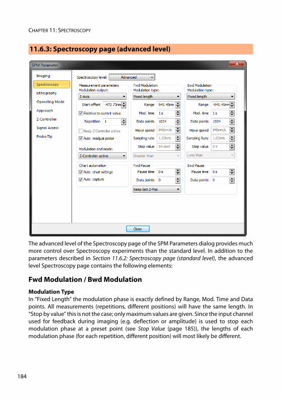
CHAPTER 11: SPECTROSCOPY
18
The advanced level of the Spectroscopy page of the SPM Parameters dialog provides muchmore control over Spectroscopy experiments than the standard level. In addition to theparameters described in Section 11.6.2: Spectroscopy page (standard level), the advancedlevel Spectroscopy page contains the following elements:
Fwd Modulation / Bwd Modulation
Modulation TypeIn “Fixed Length” the modulation phase is exactly defined by Range, Mod. Time and Datapoints. All measurements (repetitions, different positions) will have the same length. In“Stop by value” this is not the case; only maximum values are given. Since the input channelused for feedback during imaging (e.g. deflection or amplitude) is used to stop eachmodulation phase at a preset point (see Stop Value (page 185)), the lengths of eachmodulation phase (for each repetition, different position) will most likely be different.
11.6.3: Spectroscopy page (advanced level)
4
SPM PARAMETERS DIALOG
RangeIn “Fixed length” modulation, this value defines the change of the output value during themodulation phase. For forward modulation it starts from Start offset. The range can bepositive or negative (also see IMPORTANT (page 181)). For the backward modulation itstarts from the last value of the forward pause phase and with its own Range settings.Therefore, the modulation output value at the end of the backward modulation phase canbe different from the start value of the forward phase. In “Stop by value” modulation, thisfield shows a maximum value, calculated from the Data points, Move speed, and Samplingrate parameters (see below).
Mod. timeIn “Fixed length” modulation, this value defines the time used to move over the modulationrange during the respective modulation phase. In “Stop by value” modulation, this fieldshows a maximum value, calculated from the Data points and Sampling rate parameters(see below).
Data pointsThis value defines how many data points will be measured during the respectivemodulation phase. Data points will be equally distributed over the entire modulationrange. In “Fixed length” modulation, the number of data points are exactly defined by thisvalue. In “Stop by value” modulation, this is the maximum is number of datapoints that willbe recorded.
Move speedIn “Stop by value” modulation, this value defines the speed at which the modulationoutput is changed. The move speed can be positive or negative (also see IMPORTANT (page181)). For the backward modulation it can have a different value than for the forwardmodulation. Therefore the modulation output value at the end of the backwardmodulation phase can be different from the start value (Start offset). In “Fixed length”modulation mode, this value is calculated from the Range and Mod. time parameters (seeabove).
Sampling rateIn ”Stop by value” modulation, this value (in Hz) defines the number of data pointsmeasured per second during the respective modulation phase. In “Fixed length”modulation, this value is calculated form the Data points and Mod. time parameters.
Stop ValueIn “Stop by value” modulation, this value defines the abort criterion that has to be reachedin order to stop the respective modulation phase. The signal which is monitored is the Z-controller input signal (e.g. deflection or amplitude) and depends on the selectedOperating mode. The value may be positive or negative. In “Fixed length” modulationmode the value shown here has no meaning.
185
CHAPTER 11: SPECTROSCOPY
18
Stop ModeIf “Greater than” is selected the modulation is stopped if the measured value is morepositive than “Stop value”. If “Less than” is selected the measured value has to be morenegative. For Z-Axis modulations, “Greater than” should be selected for Static operatingmodes and “Less than” for Dynamic operating modes.
Fwd Pause / Bwd Pause
Pause timeThis value defines the waiting time after the respective modulation phase before the nextphase is initiated.
Data PointsThis value defines the number of data points that will be recorded during the respectivepause phase. The number of data point recorded during a pause phase can be differentfrom the number of data points recorded during the respective modulation phase. If set tozero, the respective Pause time will be automatically set to zero as well (and vice-versa).
Z-Axis Pause ModeIn “Z-Axis Modulation” Mode (see Modulation Output (page 181)), it is possible to select thePause-Phase behavior via this selector. With “Keep last Z-Pos” it maintains the final value ofthe modulation phase. With “Z-Controller active” it activates Z-controller feedback duringthe pause; the surface is tracked.
6

CHAPTER 12:
Lithography
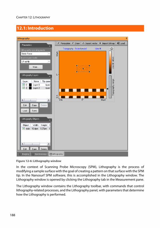
CHAPTER 12: LITHOGRAPHY
18
In the context of Scanning Probe Microscopy (SPM), Lithography is the process ofmodifying a sample surface with the goal of creating a pattern on that surface with the SPMtip. In the Nanosurf SPM software, this is accomplished in the Lithography window. TheLithography window is opened by clicking the Lithography tab in the Measurement pane.
The Lithography window contains the Lithography toolbar, with commands that controllithography-related processes, and the Lithography panel, with parameters that determinehow the Lithography is performed.
Figure 12-6: Lithography window
12.1: Introduction
8
PERFORMING LITHOGRAPHY
By default, the Lithography window also contains the Lithography Preview display (seeSection 12.6: Lithography preview (page 204)) and a Color map chart of the currentTopography measurement. The Lithography window can however display more charts,should this be desirable. For more information on adding and changing charts, see Section13.3.1: Working with multiple charts (page 211).
Lithography can be performed provided that suitable samples, tips, and lithographyparameters are used. Depending on the operating mode and operating parameters usedduring the Lithography process, the surface modifications fall into two distinct categories: 1. Mechanical surface modification through “scratching”, “indenting” (both Static Force
mode), or through “hammering” (Dynamic Force mode). This type of modificationrequire higher tip-sample interactions then normally used during imaging tomechanically transfer the desired pattern into the sample surface. The width anddepth of the scratches or indentations made mainly depend on the force exerted onthe cantilever tip and on the tip’s shape.
2. Electrochemical surface modification through voltage-dependent surface reactions.This type of modification requires a voltage difference between sample and tip, andwill add molecules to the surface (e.g. through oxidation). The width and height of theoxidative surface modifications depend on the relative humidity of the ambient air, onthe strength of the electric field, and on the tip speed.
A typical lithography process is performed as follows: 1. The sample surface is imaged to identify an area that is suitable for transfer of a
pattern. Suitable areas should preferentially be flat and dust-free. 2. The Lithography window is opened and the “Load” button of the Lithography toolbar
is clicked to import the imaged sample surface.3. A pattern that was previously designed is imported. Suitable sources for patterns can
either be (multi-layered) vector graphics files (GDS II, DXF, CIF, OAS, OASIS) or (multi-color/grayscale) pixel graphics files (BMP, DIB, GIF, TIFF, PNG, JPEG). After import of avector or pixel graphics file, the pattern is referred to as a “Lithography object” in theLithography window.
IMPORTANTLithography of objects drawn by hand and direct manipulation of the tip is available asstandard. Issuing of lithography commands through the Scripting Interface requires alicense for the Scripting Interface. Import of vector or pixel graphics files to be used aspatterns in the lithography process requires the licensed Lithography Option. Forinformation on how to activate the scripting interface or the Lithography Option, referto Access Code (page 249).
12.2: Performing lithography
189
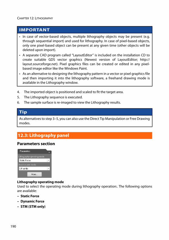
CHAPTER 12: LITHOGRAPHY
19
4. The imported object is positioned and scaled to fit the target area. 5. The Lithography sequence is executed. 6. The sample surface is re-imaged to view the Lithography results.
Parameters section
Lithography operating mode Used to select the operating mode during lithography operation:. The following optionsare available: – Static Force– Dynamic Force– STM (STM only)
IMPORTANT • In case of vector-based objects, multiple lithography objects may be present (e.g.
through sequential import) and used for lithography. In case of pixel-based objects,only one pixel-based object can be present at any given time (other objects will bedeleted upon import).
• A separate CAD program called “LayoutEditor” is included on the installation CD tocreate suitable GDS vector graphics (Newest version of LayoutEditor; http://layout.sourceforge.net). Pixel graphics files can be created or edited in any pixel-based image editor like the Windows Paint.
• As an alternative to designing the lithography pattern in a vector or pixel graphics fileand then importing it into the lithography software, a freehand drawing mode isavailable in the Lithography window.
TipAs alternatives to step 3–5, you can also use the Direct Tip Manipulation or Free Drawingmodes.
12.3: Lithography panel
0
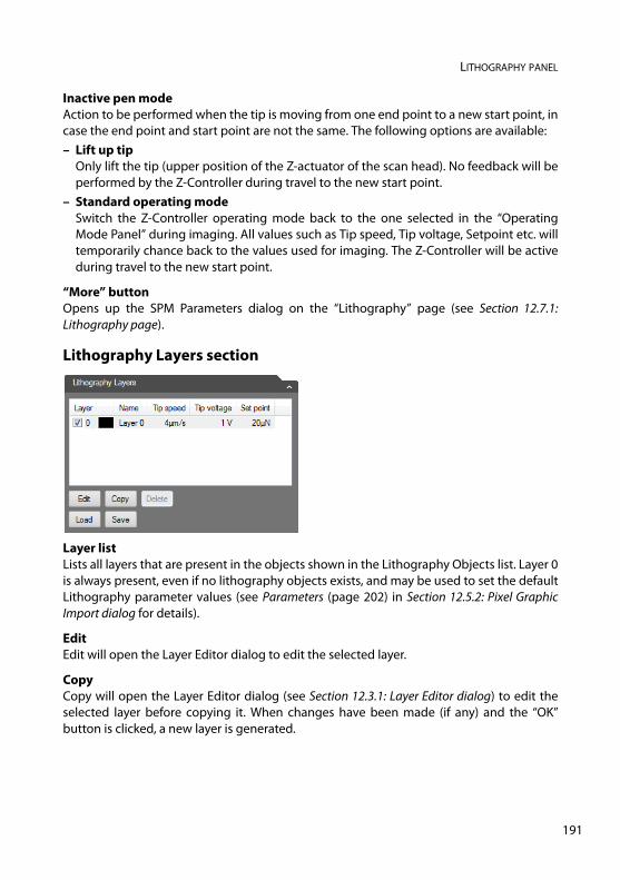
LITHOGRAPHY PANEL
Inactive pen mode Action to be performed when the tip is moving from one end point to a new start point, incase the end point and start point are not the same. The following options are available: – Lift up tip
Only lift the tip (upper position of the Z-actuator of the scan head). No feedback will beperformed by the Z-Controller during travel to the new start point.
– Standard operating modeSwitch the Z-Controller operating mode back to the one selected in the “OperatingMode Panel” during imaging. All values such as Tip speed, Tip voltage, Setpoint etc. willtemporarily chance back to the values used for imaging. The Z-Controller will be activeduring travel to the new start point.
“More” buttonOpens up the SPM Parameters dialog on the “Lithography” page (see Section 12.7.1:Lithography page).
Lithography Layers section
Layer list Lists all layers that are present in the objects shown in the Lithography Objects list. Layer 0is always present, even if no lithography objects exists, and may be used to set the defaultLithography parameter values (see Parameters (page 202) in Section 12.5.2: Pixel GraphicImport dialog for details).
Edit Edit will open the Layer Editor dialog to edit the selected layer.
CopyCopy will open the Layer Editor dialog (see Section 12.3.1: Layer Editor dialog) to edit theselected layer before copying it. When changes have been made (if any) and the “OK”button is clicked, a new layer is generated.
191
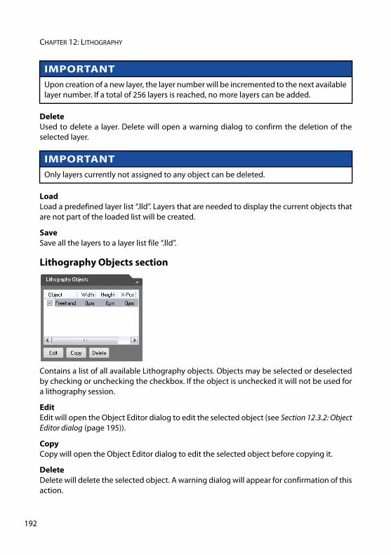
CHAPTER 12: LITHOGRAPHY
19
DeleteUsed to delete a layer. Delete will open a warning dialog to confirm the deletion of theselected layer.
LoadLoad a predefined layer list “.lld”. Layers that are needed to display the current objects thatare not part of the loaded list will be created.
SaveSave all the layers to a layer list file “.lld”.
Lithography Objects section
Contains a list of all available Lithography objects. Objects may be selected or deselectedby checking or unchecking the checkbox. If the object is unchecked it will not be used fora lithography session.
EditEdit will open the Object Editor dialog to edit the selected object (see Section 12.3.2: ObjectEditor dialog (page 195)).
CopyCopy will open the Object Editor dialog to edit the selected object before copying it.
Delete Delete will delete the selected object. A warning dialog will appear for confirmation of thisaction.
IMPORTANTUpon creation of a new layer, the layer number will be incremented to the next availablelayer number. If a total of 256 layers is reached, no more layers can be added.
IMPORTANTOnly layers currently not assigned to any object can be deleted.
2
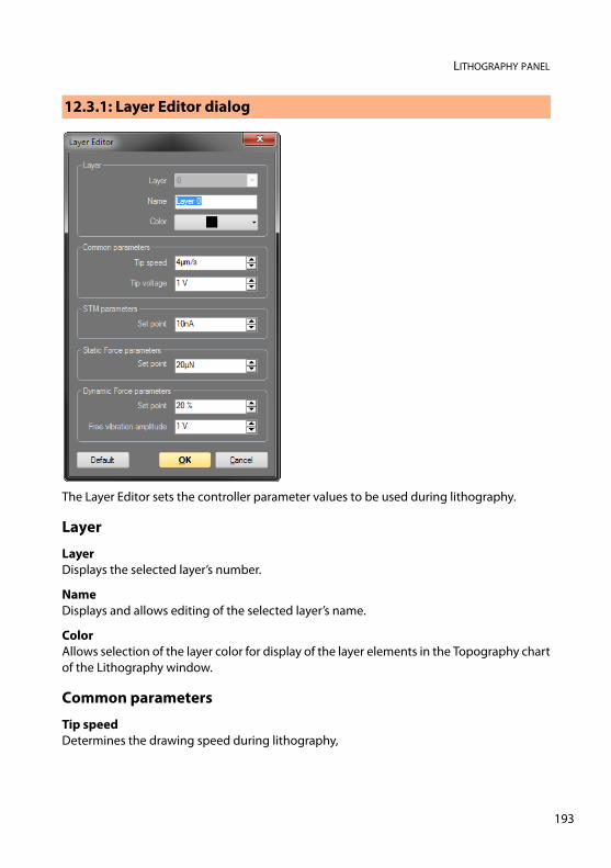
LITHOGRAPHY PANEL
The Layer Editor sets the controller parameter values to be used during lithography.
Layer
LayerDisplays the selected layer’s number.
NameDisplays and allows editing of the selected layer’s name.
ColorAllows selection of the layer color for display of the layer elements in the Topography chartof the Lithography window.
Common parameters
Tip speedDetermines the drawing speed during lithography,
12.3.1: Layer Editor dialog
193
CHAPTER 12: LITHOGRAPHY
19
Tip voltageDetermines the voltage set to the tip during oxidative Lithography.
STM parameters
SetpointUsed to set the tunnelling current Setpoint of the Z-Controller during STM Lithography.
Static Force parameters
SetpointUsed to set the force Setpoint of a lithography sequence performed in the Static Force AFMmode.
Dynamic Force parameters
SetpointUsed to set the amplitude Setpoint of a lithography sequence performed in Dynamic ForceAFM mode.
Free vibration amplitudeUsed to set the Free vibration amplitude of a lithography sequence performed in DynamicMode
“Default” buttonLoads the default Lithography parameter values.
4
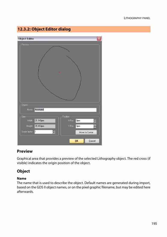
LITHOGRAPHY PANEL
Preview
Graphical area that provides a preview of the selected Lithography object. The red cross (ifvisible) indicates the origin position of the object.
Object
Name The name that is used to describe the object. Default names are generated during import,based on the GDS II object names, or on the pixel graphic filename, but may be edited hereafterwards.
12.3.2: Object Editor dialog
195
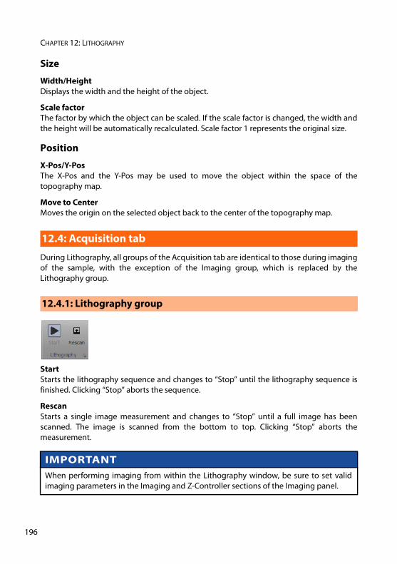
CHAPTER 12: LITHOGRAPHY
19
Size
Width/Height Displays the width and the height of the object.
Scale factor The factor by which the object can be scaled. If the scale factor is changed, the width andthe height will be automatically recalculated. Scale factor 1 represents the original size.
Position
X-Pos/Y-Pos The X-Pos and the Y-Pos may be used to move the object within the space of thetopography map.
Move to Center Moves the origin on the selected object back to the center of the topography map.
During Lithography, all groups of the Acquisition tab are identical to those during imagingof the sample, with the exception of the Imaging group, which is replaced by theLithography group.
StartStarts the lithography sequence and changes to “Stop” until the lithography sequence isfinished. Clicking “Stop” aborts the sequence.
RescanStarts a single image measurement and changes to “Stop” until a full image has beenscanned. The image is scanned from the bottom to top. Clicking “Stop” aborts themeasurement.
12.4: Acquisition tab
12.4.1: Lithography group
IMPORTANT When performing imaging from within the Lithography window, be sure to set validimaging parameters in the Imaging and Z-Controller sections of the Imaging panel.
6
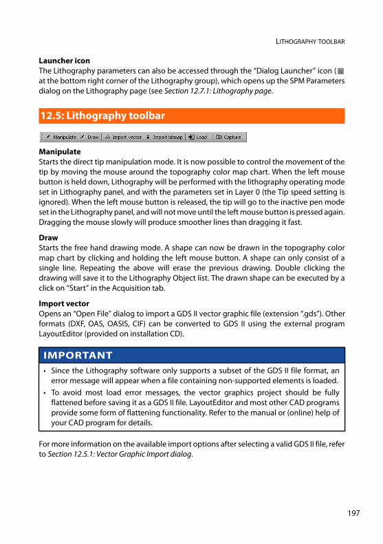
LITHOGRAPHY TOOLBAR
Launcher iconThe Lithography parameters can also be accessed through the “Dialog Launcher” icon (at the bottom right corner of the Lithography group), which opens up the SPM Parametersdialog on the Lithography page (see Section 12.7.1: Lithography page.
ManipulateStarts the direct tip manipulation mode. It is now possible to control the movement of thetip by moving the mouse around the topography color map chart. When the left mousebutton is held down, Lithography will be performed with the lithography operating modeset in Lithography panel, and with the parameters set in Layer 0 (the Tip speed setting isignored). When the left mouse button is released, the tip will go to the inactive pen modeset in the Lithography panel, and will not move until the left mouse button is pressed again.Dragging the mouse slowly will produce smoother lines than dragging it fast.
DrawStarts the free hand drawing mode. A shape can now be drawn in the topography colormap chart by clicking and holding the left mouse button. A shape can only consist of asingle line. Repeating the above will erase the previous drawing. Double clicking thedrawing will save it to the Lithography Object list. The drawn shape can be executed by aclick on “Start” in the Acquisition tab.
Import vectorOpens an “Open File” dialog to import a GDS II vector graphic file (extension “.gds”). Otherformats (DXF, OAS, OASIS, CIF) can be converted to GDS II using the external programLayoutEditor (provided on installation CD).
For more information on the available import options after selecting a valid GDS II file, referto Section 12.5.1: Vector Graphic Import dialog.
12.5: Lithography toolbar
IMPORTANT• Since the Lithography software only supports a subset of the GDS II file format, an
error message will appear when a file containing non-supported elements is loaded.• To avoid most load error messages, the vector graphics project should be fully
flattened before saving it as a GDS II file. LayoutEditor and most other CAD programsprovide some form of flattening functionality. Refer to the manual or (online) help ofyour CAD program for details.
197
CHAPTER 12: LITHOGRAPHY
19
Import bitmapOpens a “Open File” dialog for importing a BMP, DIB, GIF, TIFF, PNG, or JPEG pixel graphicsfile.
For more information on the available import options after selecting a valid pixel graphicsfile, refer to Section 12.5.2: Pixel Graphic Import dialog.
LoadLoads the Topography image from the Imaging window into the Lithography Topographychart.
CaptureThis button captures the measurement currently displayed in the “Lithography window” tothe History page of the Gallery panel. If clicked during a measurement, a copy is generatedas soon as the measurement in progress is finished. The capture process is cancelled byclicking second time. The captured measurement is stored as a new document and remainsopen in the Document space of the SPM Control Software.
IMPORTANTThe Lithography software supports files with 256 pixels or less in width and height.
8
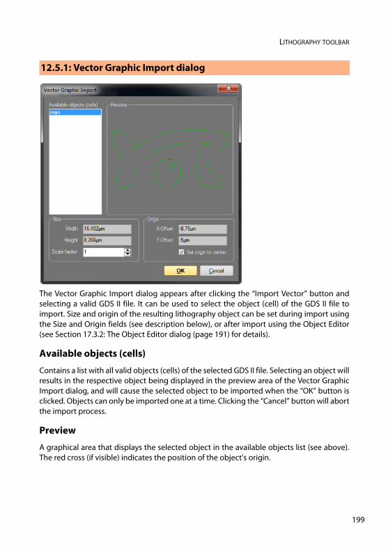
LITHOGRAPHY TOOLBAR
The Vector Graphic Import dialog appears after clicking the “Import Vector” button andselecting a valid GDS II file. It can be used to select the object (cell) of the GDS II file toimport. Size and origin of the resulting lithography object can be set during import usingthe Size and Origin fields (see description below), or after import using the Object Editor(see Section 17.3.2: The Object Editor dialog (page 191) for details).
Available objects (cells)
Contains a list with all valid objects (cells) of the selected GDS II file. Selecting an object willresults in the respective object being displayed in the preview area of the Vector GraphicImport dialog, and will cause the selected object to be imported when the “OK” button isclicked. Objects can only be imported one at a time. Clicking the “Cancel” button will abortthe import process.
Preview
A graphical area that displays the selected object in the available objects list (see above).The red cross (if visible) indicates the position of the object's origin.
12.5.1: Vector Graphic Import dialog
199
CHAPTER 12: LITHOGRAPHY
20
Size
Width / Height Displays width and height of the selected object (cell).
Scale factor The factor by which the selected object (cell) will be scaled. A scale factor of 1 correspondsto the original object size. If the scale factor is changed manually, the object's width andheight will be recalculated and displayed automatically.
Origin
X-Offset / Y-Offset The X-Offset and the Y-Offset of the origin of the selected object (cell).
Set origin to centerWhen enabled, the origin of the object (cell) will be set to the center of the rectangle thatencloses the object. When disabled, the origin will remain at the position that is defined inthe object.
0
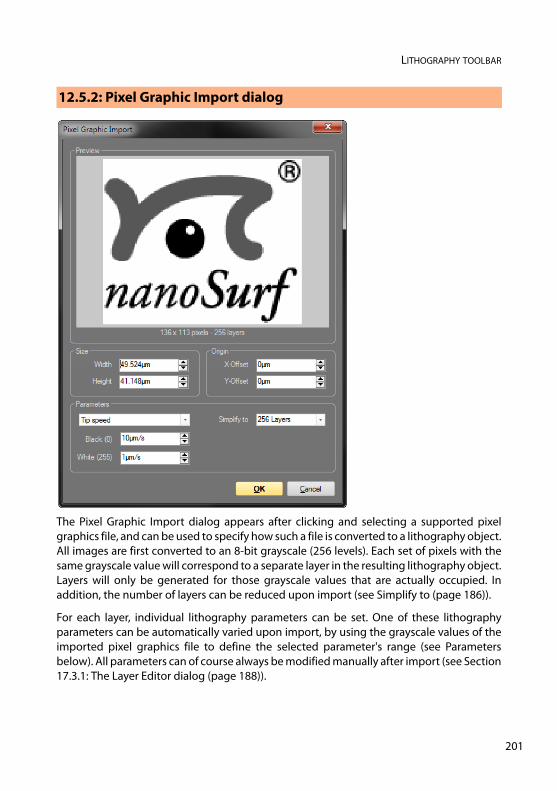
LITHOGRAPHY TOOLBAR
The Pixel Graphic Import dialog appears after clicking and selecting a supported pixelgraphics file, and can be used to specify how such a file is converted to a lithography object.All images are first converted to an 8-bit grayscale (256 levels). Each set of pixels with thesame grayscale value will correspond to a separate layer in the resulting lithography object.Layers will only be generated for those grayscale values that are actually occupied. Inaddition, the number of layers can be reduced upon import (see Simplify to (page 186)).
For each layer, individual lithography parameters can be set. One of these lithographyparameters can be automatically varied upon import, by using the grayscale values of theimported pixel graphics file to define the selected parameter's range (see Parametersbelow). All parameters can of course always be modified manually after import (see Section17.3.1: The Layer Editor dialog (page 188)).
12.5.2: Pixel Graphic Import dialog
201
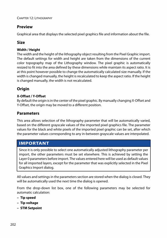
CHAPTER 12: LITHOGRAPHY
20
Preview
Graphical area that displays the selected pixel graphics file and information about the file.
Size
Width / Height The width and the height of the lithography object resulting from the Pixel Graphic import.The default settings for width and height are taken from the dimensions of the currentcolor topography map of the Lithography window. The pixel graphic is automaticallyresized to fit into the area defined by these dimensions while maintain its aspect ratio. It isat this point however possible to change the automatically calculated size manually. If thewidth is changed manually, the height is recalculated to keep the aspect ratio. If the heightis changed manually, the width is not recalculated.
Origin
X-Offset / Y-Offset By default the origin is in the center of the pixel graphic. By manually changing X-Offset andY-Offset, the origin may be moved to a different position.
Parameters
This area allows selection of the lithography parameter that will be automatically varied,based on the different grayscale values of the imported pixel graphics file. The parametervalues for the black and white pixels of the imported pixel graphic can be set, after whichthe parameter values corresponding to any in-between grayscale values are interpolated.
All values and settings in the parameters section are stored when the dialog is closed. Theywill be automatically used the next time the dialog is opened.
From the drop-down list box, one of the following parameters may be selected forautomatic calculation: – Tip speed – Tip voltage – STM Setpoint
IMPORTANT Since it is only possible to select one automatically adjusted lithography parameter perimport, the other parameters must be set elsewhere. This is achieved by setting theLayer 0 parameters before import. The values entered here will be used as default valuesfor all imported layers, except for the parameter that was explicitly selected in the PixelGraphics Import dialog.
2
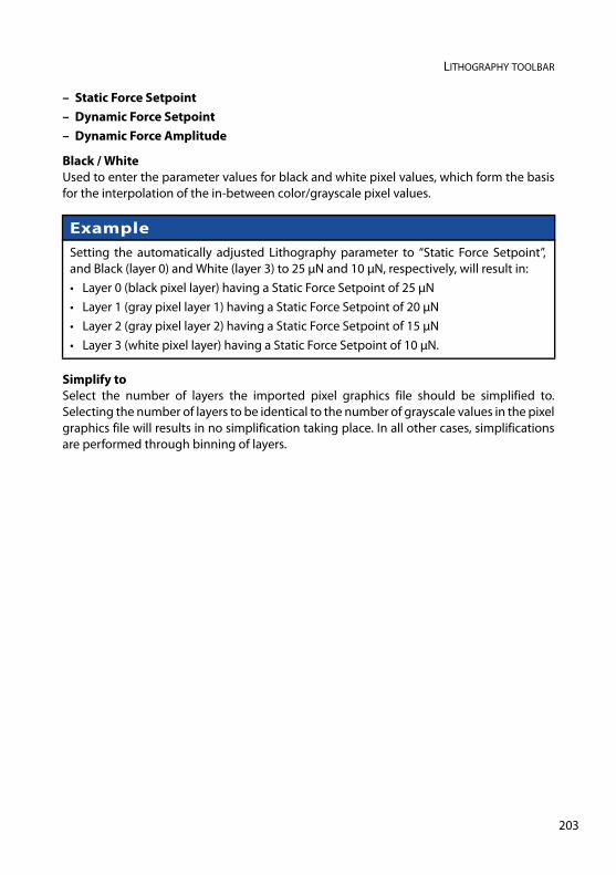
LITHOGRAPHY TOOLBAR
– Static Force Setpoint – Dynamic Force Setpoint – Dynamic Force Amplitude
Black / White Used to enter the parameter values for black and white pixel values, which form the basisfor the interpolation of the in-between color/grayscale pixel values.
Simplify to Select the number of layers the imported pixel graphics file should be simplified to.Selecting the number of layers to be identical to the number of grayscale values in the pixelgraphics file will results in no simplification taking place. In all other cases, simplificationsare performed through binning of layers.
Example Setting the automatically adjusted Lithography parameter to “Static Force Setpoint”,and Black (layer 0) and White (layer 3) to 25 μN and 10 μN, respectively, will result in:• Layer 0 (black pixel layer) having a Static Force Setpoint of 25 μN• Layer 1 (gray pixel layer 1) having a Static Force Setpoint of 20 μN• Layer 2 (gray pixel layer 2) having a Static Force Setpoint of 15 μN• Layer 3 (white pixel layer) having a Static Force Setpoint of 10 μN.
203
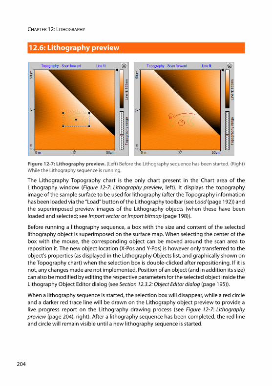
CHAPTER 12: LITHOGRAPHY
20
The Lithography Topography chart is the only chart present in the Chart area of theLithography window (Figure 12-7: Lithography preview, left). It displays the topographyimage of the sample surface to be used for lithography (after the Topography informationhas been loaded via the “Load” button of the Lithography toolbar (see Load (page 192)) andthe superimposed preview images of the Lithography objects (when these have beenloaded and selected; see Import vector or Import bitmap (page 198)).
Before running a lithography sequence, a box with the size and content of the selectedlithography object is superimposed on the surface map. When selecting the center of thebox with the mouse, the corresponding object can be moved around the scan area toreposition it. The new object location (X-Pos and Y-Pos) is however only transferred to theobject's properties (as displayed in the Lithography Objects list, and graphically shown onthe Topography chart) when the selection box is double-clicked after repositioning. If it isnot, any changes made are not implemented. Position of an object (and in addition its size)can also be modified by editing the respective parameters for the selected object inside theLithography Object Editor dialog (see Section 12.3.2: Object Editor dialog (page 195)).
When a lithography sequence is started, the selection box will disappear, while a red circleand a darker red trace line will be drawn on the Lithography object preview to provide alive progress report on the Lithography drawing process (see Figure 12-7: Lithographypreview (page 204), right). After a lithography sequence has been completed, the red lineand circle will remain visible until a new lithography sequence is started.
12.6: Lithography preview
Figure 12-7: Lithography preview. (Left) Before the Lithography sequence has been started. (Right)While the Lithography sequence is running.
4
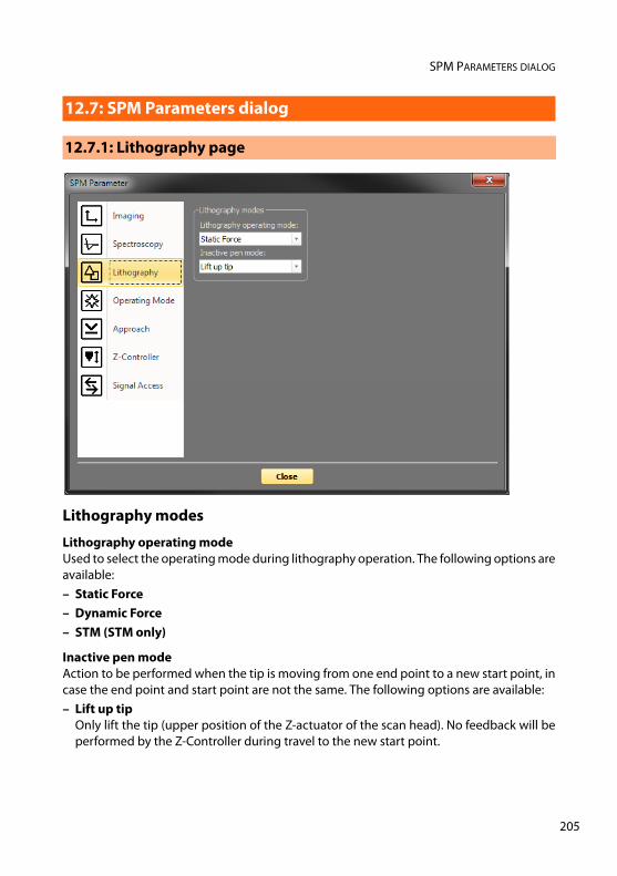
SPM PARAMETERS DIALOG
Lithography modes
Lithography operating mode Used to select the operating mode during lithography operation. The following options areavailable: – Static Force– Dynamic Force – STM (STM only)
Inactive pen mode Action to be performed when the tip is moving from one end point to a new start point, incase the end point and start point are not the same. The following options are available: – Lift up tip
Only lift the tip (upper position of the Z-actuator of the scan head). No feedback will beperformed by the Z-Controller during travel to the new start point.
12.7: SPM Parameters dialog
12.7.1: Lithography page
205
CHAPTER 12: LITHOGRAPHY
20
– Standard operating modeSwitch the Z-Controller operating mode back to the one selected in the “OperatingMode Panel” during imaging. All values such as Tip speed, Tip voltage, Setpoint etc. willtemporarily chance back to the values used for imaging. The Z-Controller will be activeduring travel to the new start point.
Chart automation
Auto chart settingsIf checked, the chart arrangement is automatically updated (see also Auto chart settings(page 206)).
Auto CaptureIf checked, all Lithography measurements are automatically stored in the history Gallery. Ifunchecked, you have to click the “Capture” button in the Lithography tool bar to manuallysave your measurement data.
6

CHAPTER 13:
Working with documents0
0
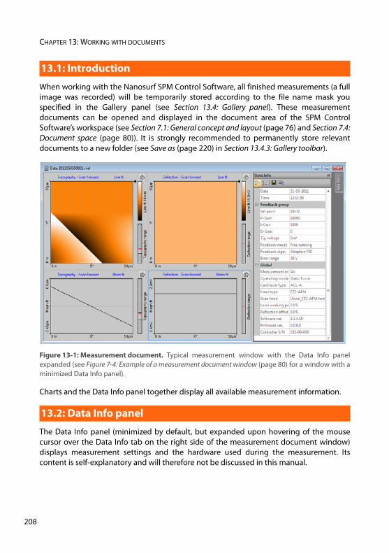
CHAPTER 13: WORKING WITH DOCUMENTS
20
When working with the Nanosurf SPM Control Software, all finished measurements (a fullimage was recorded) will be temporarily stored according to the file name mask youspecified in the Gallery panel (see Section 13.4: Gallery panel). These measurementdocuments can be opened and displayed in the document area of the SPM ControlSoftware’s workspace (see Section 7.1: General concept and layout (page 76) and Section 7.4:Document space (page 80)). It is strongly recommended to permanently store relevantdocuments to a new folder (see Save as (page 220) in Section 13.4.3: Gallery toolbar).
Charts and the Data Info panel together display all available measurement information.
The Data Info panel (minimized by default, but expanded upon hovering of the mousecursor over the Data Info tab on the right side of the measurement document window)displays measurement settings and the hardware used during the measurement. Itscontent is self-explanatory and will therefore not be discussed in this manual.
13.1: Introduction
Figure 13-1: Measurement document. Typical measurement window with the Data Info panelexpanded (see Figure 7-4: Example of a measurement document window (page 80) for a window with aminimized Data Info panel).
13.2: Data Info panel
8
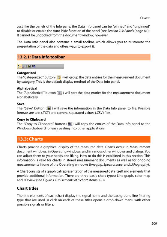
CHARTS
Just like the panels of the Info pane, the Data Info panel can be “pinned” and “unpinned”to disable or enable the Auto-hide function of the panel (see Section 7.5: Panels (page 81)).It cannot be undocked from the document window, however.
The Data Info panel also contains a small toolbar, which allows you to customize thepresentation of the data and offers ways to export it.
CategorizedThe “Categorized” button ( ) will group the data entries for the measurement documentby category. This is the default display method of the Data Info panel.
AlphabeticalThe “Alphabetical” button ( ) will sort the data entries for the measurement documentalphabetically.
SaveThe “Save” button ( ) will save the information in the Data Info panel to file. Possibleformats are text (.TXT) and comma separated values (.CSV) files.
Copy to ClipboardThe “Copy to Clipboard” button ( ) will copy the entries of the Data Info panel to theWindows clipboard for easy pasting into other applications.
Charts provide a graphical display of the measured data. Charts occur in Measurementdocument windows, in Operating windows, and in various other windows and dialogs. Youcan adjust them to your needs and liking. How to do this is explained in this section. Thisinformation is valid for charts in stored measurement documents as well as for ongoingmeasurements in one of the Operating windows (Imaging, Spectroscopy, and Lithography).
A Chart consists of a graphical representation of the measured data itself and elements thatprovide additional information. There are three basic chart types: Line graph, color mapand 3D view (see Figure 13-2: Elements of a chart, items 1–3).
Chart titles
The title elements of each chart display the signal name and the background line filteringtype that are used. A click on each of these titles opens a drop-down menu with otherpossible signals or filters:
13.2.1: Data Info toolbar
13.3: Charts
209
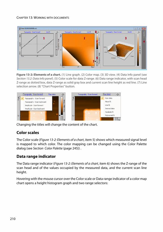
CHAPTER 13: WORKING WITH DOCUMENTS
21
Changing the titles will change the content of the chart.
Color scales
The Color scale (Figure 13-2: Elements of a chart, item 5) shows which measured signal levelis mapped to which color. The color mapping can be changed using the Color Palettedialog (see Section Color Palette (page 245)) .
Data range indicator
The Data range indicator (Figure 13-2: Elements of a chart, item 6) shows the Z-range of thescan head and of the values occupied by the measured data, and the current scan lineheight.
Hovering with the mouse cursor over the Color scale or Data range indicator of a color mapchart opens a height histogram graph and two range selectors:
Figure 13-2: Elements of a chart. (1) Line graph. (2) Color map. (3) 3D view. (4) Data Info panel (seeSection 13.2: Data Info panel). (5) Color scale for data Z-range. (6) Data range indicator, with scan headZ-range as dotted box, data Z-range as solid gray box and current scan line height as red line. (7) Lineselection arrow. (8) “Chart Properties” button.
11 2222 334455555
6666677777
88
0
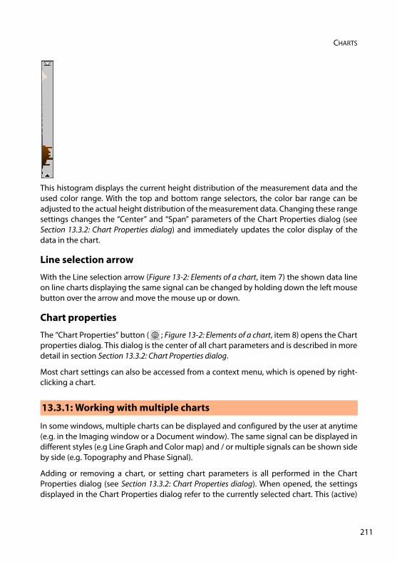
CHARTS
This histogram displays the current height distribution of the measurement data and theused color range. With the top and bottom range selectors, the color bar range can beadjusted to the actual height distribution of the measurement data. Changing these rangesettings changes the “Center” and “Span” parameters of the Chart Properties dialog (seeSection 13.3.2: Chart Properties dialog) and immediately updates the color display of thedata in the chart.
Line selection arrow
With the Line selection arrow (Figure 13-2: Elements of a chart, item 7) the shown data lineon line charts displaying the same signal can be changed by holding down the left mousebutton over the arrow and move the mouse up or down.
Chart properties
The “Chart Properties” button ( ; Figure 13-2: Elements of a chart, item 8) opens the Chartproperties dialog. This dialog is the center of all chart parameters and is described in moredetail in section Section 13.3.2: Chart Properties dialog.
Most chart settings can also be accessed from a context menu, which is opened by right-clicking a chart.
In some windows, multiple charts can be displayed and configured by the user at anytime(e.g. in the Imaging window or a Document window). The same signal can be displayed indifferent styles (e.g Line Graph and Color map) and / or multiple signals can be shown sideby side (e.g. Topography and Phase Signal).
Adding or removing a chart, or setting chart parameters is all performed in the ChartProperties dialog (see Section 13.3.2: Chart Properties dialog). When opened, the settingsdisplayed in the Chart Properties dialog refer to the currently selected chart. This (active)
13.3.1: Working with multiple charts
211
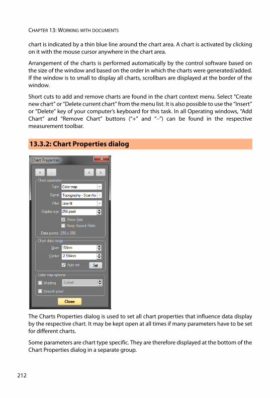
CHAPTER 13: WORKING WITH DOCUMENTS
21
chart is indicated by a thin blue line around the chart area. A chart is activated by clickingon it with the mouse cursor anywhere in the chart area.
Arrangement of the charts is performed automatically by the control software based onthe size of the window and based on the order in which the charts were generated/added.If the window is to small to display all charts, scrollbars are displayed at the border of thewindow.
Short cuts to add and remove charts are found in the chart context menu. Select “Createnew chart” or “Delete current chart” from the menu list. It is also possible to use the “Insert”or “Delete” key of your computer’s keyboard for this task. In all Operating windows, “AddChart“ and “Remove Chart” buttons (“+” and “–”) can be found in the respectivemeasurement toolbar.
The Charts Properties dialog is used to set all chart properties that influence data displayby the respective chart. It may be kept open at all times if many parameters have to be setfor different charts.
Some parameters are chart type specific. They are therefore displayed at the bottom of theChart Properties dialog in a separate group.
13.3.2: Chart Properties dialog
2
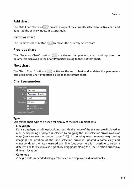
CHARTS
Add chart
The “Add Chart” button ( ) creates a copy of the currently selected or active chart andadds it to the active window in last position.
Remove chart
The “Remove Chart” button ( ) removes the currently active chart.
Previous chart
The “Previous Chart” button ( ) activates the previous chart and updates theparameters displayed in the Chart Properties dialog to those of that chart.
Next chart
The “Next Chart” button ( ) activates the next chart and updates the parametersdisplayed in the Chart Properties dialog to those of that chart.
Chart parameters
TypeSelects the chart type to be used for display of the measurement data:– Line graph
Data is displayed as a line plot. Points outside the range of the scanner are displayed inred. The line being displayed is selected by dragging the Line selection arrow in a Colormap (see Line selection arrow (page 211)). In ongoing measurements (e.g. duringimaging) the position of the Line selection arrow is updated automatically andcorresponds to the last measured scan line (but even here it is possible to select adifferent line for view in a line graph by dragging/holding the Line selection arrow in adifferent location).
– Color mapZ-height data is encoded using a color scale and displayed 2-dimensionally.
213
CHAPTER 13: WORKING WITH DOCUMENTS
21
– 3D viewData is shown in a 3-dimensional representation in parallel perspective. Colorinformation (such as implemented in the Color map) is maintained.
SignalSelects the input channel (signal data) to be used for the chart. The available signalsdepend on the operating mode (selected or used) and the status of the User inputs.
FilterSelects the line filter method. The control software applies this filter to the measured databefore displaying it (see Figure 13-3: Data filter types). No modification of the originalmeasurement data occurs (selecting another filter is always possible). Available data filtersare:– Raw data
No data processing.– Mean fit
Calculates the mean value of each line of data points and subtracts this number from theraw measurement data for each data point of that line.
– Line fitCalculates the first order least squares fit (mean value and slope) for each line of datapoints and subtracts the fitted values from the raw measurement data for each datapoint of that line.
– Derived dataCalculates the difference between two consecutive data points (derivative) and displaysthis instead of the raw image data.
– Parabola fitCalculates the second order least squares fit for each line of data points and subtracts thefitted values from the raw measurement data for each data point of that line.
– Polynomial fitCalculates the fourth order least squares fit for each line of data points and subtracts thefitted values from the raw measurement data for each data point of that line.
Display sizeThe size of the chart in pixels.
Show AxisWhen checked (default), the axis labels, color and range scales, and titles are displayedalongside the graph. When unchecked, they are hidden.
Keep Aspect ratioWhen checked, the axis in the color map are drawn in their correct size-relation (accordingto their value and unit). When unchecked (default), the size of the display is always a squareand data pixels are stretched if necessary.
4
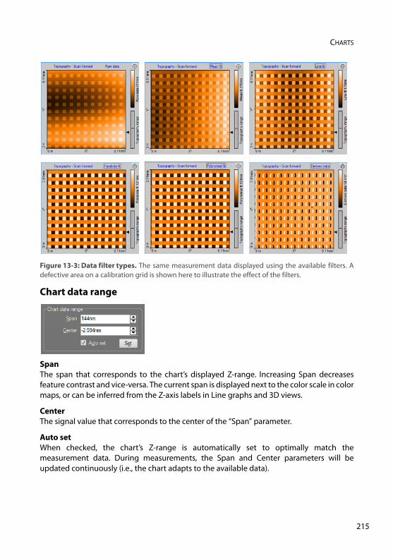
CHARTS
Chart data range
SpanThe span that corresponds to the chart’s displayed Z-range. Increasing Span decreasesfeature contrast and vice-versa. The current span is displayed next to the color scale in colormaps, or can be inferred from the Z-axis labels in Line graphs and 3D views.
CenterThe signal value that corresponds to the center of the “Span” parameter.
Auto setWhen checked, the chart’s Z-range is automatically set to optimally match themeasurement data. During measurements, the Span and Center parameters will beupdated continuously (i.e., the chart adapts to the available data).
Figure 13-3: Data filter types. The same measurement data displayed using the available filters. Adefective area on a calibration grid is shown here to illustrate the effect of the filters.
215
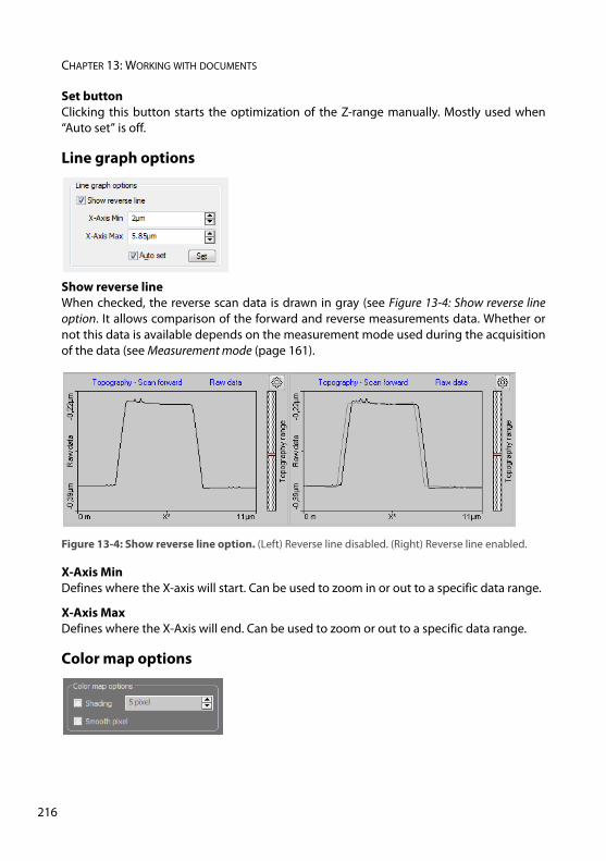
CHAPTER 13: WORKING WITH DOCUMENTS
21
Set buttonClicking this button starts the optimization of the Z-range manually. Mostly used when“Auto set” is off.
Line graph options
Show reverse lineWhen checked, the reverse scan data is drawn in gray (see Figure 13-4: Show reverse lineoption. It allows comparison of the forward and reverse measurements data. Whether ornot this data is available depends on the measurement mode used during the acquisitionof the data (see Measurement mode (page 161).
X-Axis MinDefines where the X-axis will start. Can be used to zoom in or out to a specific data range.
X-Axis MaxDefines where the X-Axis will end. Can be used to zoom or out to a specific data range.
Color map options
Figure 13-4: Show reverse line option. (Left) Reverse line disabled. (Right) Reverse line enabled.
6
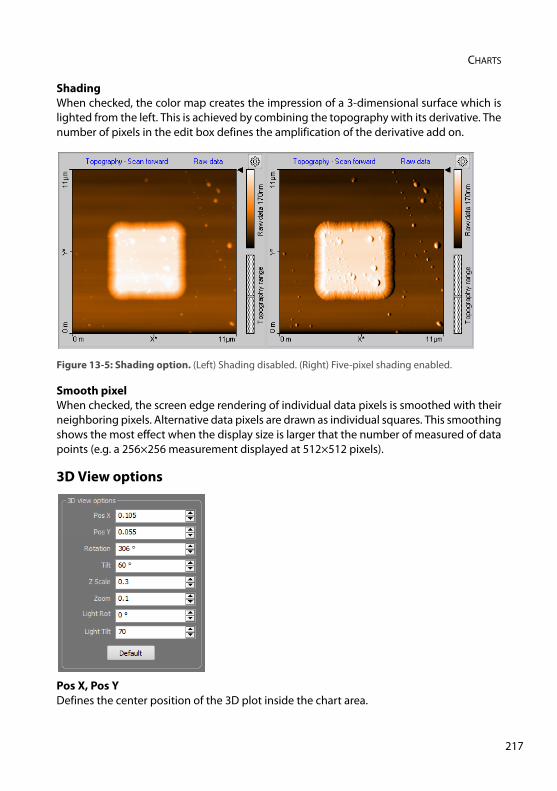
CHARTS
ShadingWhen checked, the color map creates the impression of a 3-dimensional surface which islighted from the left. This is achieved by combining the topography with its derivative. Thenumber of pixels in the edit box defines the amplification of the derivative add on.
Smooth pixelWhen checked, the screen edge rendering of individual data pixels is smoothed with theirneighboring pixels. Alternative data pixels are drawn as individual squares. This smoothingshows the most effect when the display size is larger that the number of measured of datapoints (e.g. a 256×256 measurement displayed at 512×512 pixels).
3D View options
Pos X, Pos YDefines the center position of the 3D plot inside the chart area.
Figure 13-5: Shading option. (Left) Shading disabled. (Right) Five-pixel shading enabled.
217
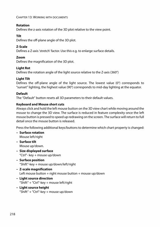
CHAPTER 13: WORKING WITH DOCUMENTS
21
RotationDefines the z-axis rotation of the 3D plot relative to the view point.
TiltDefines the off-plane angle of the 3D plot.
Z-ScaleDefines a Z-axis ‘stretch’ factor. Use this e.g. to enlarge surface details.
ZoomDefines the magnification of the 3D plot.
Light RotDefines the rotation angle of the light source relative to the Z-axis (360°)
Light TiltDefines the off-plane angle of the light source. The lowest value (0°) corresponds to“sunset” lighting, the highest value (90°) corresponds to mid-day lighting at the equator.
DefaultThe “Default” button resets all 3D parameters to their default values.
Keyboard and Mouse short cutsAlways click and hold the left mouse button on the 3D view chart while moving around themouse to change the 3D view. The surface is reduced in feature complexity once the leftmouse button is pressed to speed up redrawing on the screen. The surface will return to fulldetail once the mouse button is released.
Press the following additional keys/buttons to determine which chart property is changed:– Surface rotation
Mouse left/right– Surface tilt
Mouse up/down.– Size displayed surface
“Ctrl”- key + mouse up/down– Surface position
“Shift”-key + mouse up/down/left/right– Z-scale magnification
Left mouse button + right mouse button + mouse up/down– Light source direction
“Shift” + ”Ctrl”-key + mouse left/right– Light source height
“Shift” + ”Ctrl”-key + mouse up/down
8
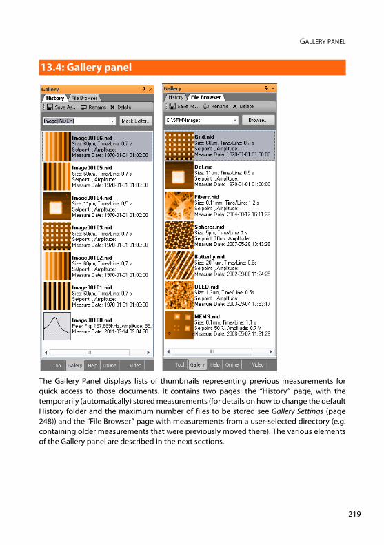
GALLERY PANEL
The Gallery Panel displays lists of thumbnails representing previous measurements forquick access to those documents. It contains two pages: the “History” page, with thetemporarily (automatically) stored measurements (for details on how to change the defaultHistory folder and the maximum number of files to be stored see Gallery Settings (page248)) and the “File Browser” page with measurements from a user-selected directory (e.g.containing older measurements that were previously moved there). The various elementsof the Gallery panel are described in the next sections.
13.4: Gallery panel
219
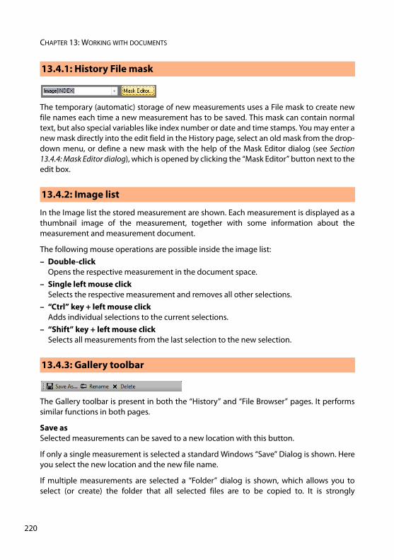
CHAPTER 13: WORKING WITH DOCUMENTS
22
The temporary (automatic) storage of new measurements uses a File mask to create newfile names each time a new measurement has to be saved. This mask can contain normaltext, but also special variables like index number or date and time stamps. You may enter anew mask directly into the edit field in the History page, select an old mask from the drop-down menu, or define a new mask with the help of the Mask Editor dialog (see Section13.4.4: Mask Editor dialog), which is opened by clicking the “Mask Editor” button next to theedit box.
In the Image list the stored measurement are shown. Each measurement is displayed as athumbnail image of the measurement, together with some information about themeasurement and measurement document.
The following mouse operations are possible inside the image list:– Double-click
Opens the respective measurement in the document space.– Single left mouse click
Selects the respective measurement and removes all other selections.– “Ctrl” key + left mouse click
Adds individual selections to the current selections.– “Shift” key + left mouse click
Selects all measurements from the last selection to the new selection.
The Gallery toolbar is present in both the “History” and “File Browser” pages. It performssimilar functions in both pages.
Save asSelected measurements can be saved to a new location with this button.
If only a single measurement is selected a standard Windows “Save” Dialog is shown. Hereyou select the new location and the new file name.
If multiple measurements are selected a “Folder” dialog is shown, which allows you toselect (or create) the folder that all selected files are to be copied to. It is strongly
13.4.1: History File mask
13.4.2: Image list
13.4.3: Gallery toolbar
0
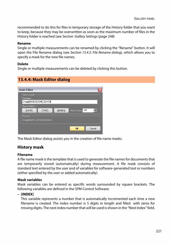
GALLERY PANEL
recommended to do this for files in temporary storage of the History folder that you wantto keep, because they may be overwritten as soon as the maximum number of files in theHistory folder is reached (see Section Gallery Settings (page 248)
RenameSingle or multiple measurements can be renamed by clicking the “Rename” button. It willopen the File Rename dialog (see Section 13.4.5: File Rename dialog), which allows you tospecify a mask for the new file names.
DeleteSingle or multiple measurements can be deleted by clicking this button.
The Mask Editor dialog assists you in the creation of file name masks.
History mask
FilenameA file name mask is the template that is used to generate the file names for documents thatare temporarily stored (automatically) during measurement. A file mask consists ofstandard text entered by the user and of variables for software-generated text or numbers(either specified by the user or added automatically).
Mask variablesMask variables can be entered as specific words surrounded by square brackets. Thefollowing variables are defined in the SPM Control Software:– [INDEX]
This variable represents a number that is automatically incremented each time a newfilename is created. The index number is 5 digits in length and filled with zeros formissing digits. The next index number that will be used is shown in the “Next Index” field.
13.4.4: Mask Editor dialog
221
CHAPTER 13: WORKING WITH DOCUMENTS
22
– [TIME]This variable represents the actual time of file name creation. It is formatted with twodigit numbers for the hours, minutes and seconds (HHMMSS). This time format is usedregardless of the Regional Settings of the Windows operating system.
– [DATE]This variable represents the date of the day the file was created (i.e., the day themeasurement was performed). It contains four digit numbers for the year and two digitnumbers for month and day (YYYYMMDD). This date format is used regardless of theRegional Settings of the Windows operating system.
To quickly insert a Mask variable at the current cursor position in the mask edit box, clickthe corresponding button.
Next IndexThis entry field defines the next index number to be used. By default this value is identicalto the highest number present in the History files, increased by one.
Preview
The filename that will be used for the next measurement document to be saved (asspecified by your entries) is shown here.
IMPORTANTIf no Mask variable is used, an index is automatically added to the text string defined inthe filename mask.
2
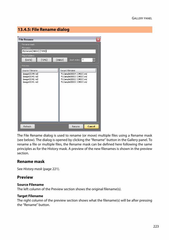
GALLERY PANEL
The File Rename dialog is used to rename (or move) multiple files using a Rename mask(see below). The dialog is opened by clicking the “Rename” button in the Gallery panel. Torename a file or multiple files, the Rename mask can be defined here following the sameprinciples as for the History mask. A preview of the new filenames is shown in the previewsection.
Rename mask
See History mask (page 221).
Preview
Source FilenameThe left column of the Preview section shows the original filename(s).
Target FilenameThe right column of the preview section shows what the filename(s) will be after pressingthe “Rename” button.
13.4.5: File Rename dialog
223
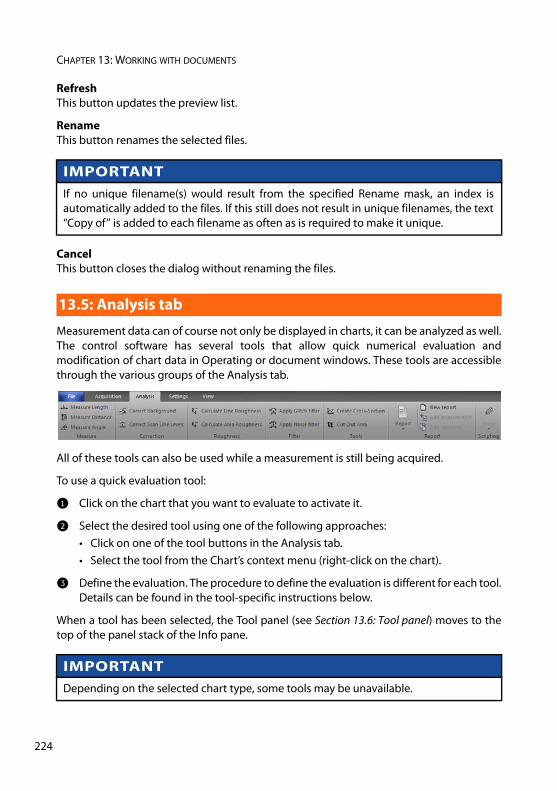
CHAPTER 13: WORKING WITH DOCUMENTS
22
RefreshThis button updates the preview list.
RenameThis button renames the selected files.
CancelThis button closes the dialog without renaming the files.
Measurement data can of course not only be displayed in charts, it can be analyzed as well.The control software has several tools that allow quick numerical evaluation andmodification of chart data in Operating or document windows. These tools are accessiblethrough the various groups of the Analysis tab.
All of these tools can also be used while a measurement is still being acquired.
To use a quick evaluation tool:
1 Click on the chart that you want to evaluate to activate it.
2 Select the desired tool using one of the following approaches: • Click on one of the tool buttons in the Analysis tab. • Select the tool from the Chart’s context menu (right-click on the chart).
3 Define the evaluation. The procedure to define the evaluation is different for each tool.Details can be found in the tool-specific instructions below.
When a tool has been selected, the Tool panel (see Section 13.6: Tool panel) moves to thetop of the panel stack of the Info pane.
IMPORTANTIf no unique filename(s) would result from the specified Rename mask, an index isautomatically added to the files. If this still does not result in unique filenames, the text“Copy of” is added to each filename as often as is required to make it unique.
13.5: Analysis tab
IMPORTANTDepending on the selected chart type, some tools may be unavailable.
4
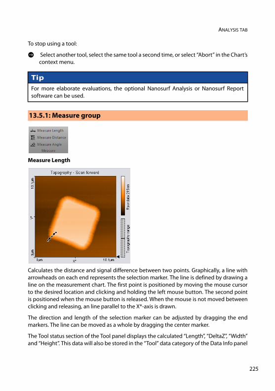
ANALYSIS TAB
To stop using a tool:
> Select another tool, select the same tool a second time, or select “Abort” in the Chart’scontext menu.
Measure Length
Calculates the distance and signal difference between two points. Graphically, a line witharrowheads on each end represents the selection marker. The line is defined by drawing aline on the measurement chart. The first point is positioned by moving the mouse cursorto the desired location and clicking and holding the left mouse button. The second pointis positioned when the mouse button is released. When the mouse is not moved betweenclicking and releasing, an line parallel to the X*-axis is drawn.
The direction and length of the selection marker can be adjusted by dragging the endmarkers. The line can be moved as a whole by dragging the center marker.
The Tool status section of the Tool panel displays the calculated “Length”, “DeltaZ”, “Width”and “Height”. This data will also be stored in the “Tool” data category of the Data Info panel
TipFor more elaborate evaluations, the optional Nanosurf Analysis or Nanosurf Reportsoftware can be used.
13.5.1: Measure group
225
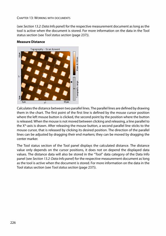
CHAPTER 13: WORKING WITH DOCUMENTS
22
(see Section 13.2: Data Info panel) for the respective measurement document as long as thetool is active when the document is stored. For more information on the data in the Toolstatus section (see Tool status section (page 237)).
Measure Distance
Calculates the distance between two parallel lines. The parallel lines are defined by drawingthem in the chart. The first point of the first line is defined by the mouse cursor positionwhere the left mouse button is clicked, the second point by the position where the buttonis released. When the mouse is not moved between clicking and releasing, a line parallel tothe X*axis is drawn. After releasing the mouse button, a second parallel line sticks to themouse cursor, that is released by clicking its desired position. The direction of the parallellines can be adjusted by dragging their end markers; they can be moved by dragging thecenter marker.
The Tool status section of the Tool panel displays the calculated distance. The distancevalue only depends on the cursor positions, it does not on depend the displayed datavalues. The distance data will also be stored in the “Tool” data category of the Data Infopanel (see Section 13.2: Data Info panel) for the respective measurement document as longas the tool is active when the document is stored. For more information on the data in theTool status section (see Tool status section (page 237)).
6
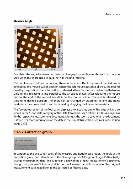
ANALYSIS TAB
Measure Angle
Calculates the angle between two lines. In Line graph-type displays, this tool can only beused when the chart displays data that has the unit “meters”.
The two lines are defined by drawing them in the chart. The first point of the first line isdefined by the mouse cursor position where the left mouse button is clicked, the secondpoint by the position where the button is released. When the mouse is not moved betweenclicking and releasing, a line parallel to the X*-axis is drawn. After releasing the mousebutton, the end of the second line sticks to the mouse pointer. The end is released byclicking its desired position. The angle can be changed by dragging the line end pointmarkers or the corner mark; it can be moved by dragging the line center markers.
The Tool status section of the Tool panel displays the calculated angle. This data will also bestored in the “Tool” data category of the Data Info panel (see Section 13.2: Data Info panel)for the respective measurement document as long as the tool is active when the documentis stored. For more information on the data in the Tool status section (see Tool status section(page 237)).
In contrast to the evaluation tools of the Measure and Roughness groups, the tools of theCorrection group (and also those of the Filter group (see Filter group (page 231)) actuallychange measurement data. This is done in a copy of the original measurement document,though, so you won’t lose any data and will always be able to access the originalmeasurement data in addition to the corrected or filtered data.
13.5.2: Correction group
227
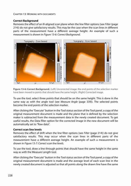
CHAPTER 13: WORKING WITH DOCUMENTS
22
Correct Background Removes the effect of an ill-aligned scan plane when the line filter options (see Filter (page214)) do not give satisfactory results. This may be the case when the scan lines in differentparts of the measurement have a different average height. An example of such ameasurement is shown in Figure 13-6: Correct Background.
To use the tool, select three points that should be on the same height. This is done in thesame way as with the angle tool (see Measure Angle (page 339)). The selected pointsbecome the end points of the selection marker.
After clicking the “Execute” button in the Tool status section of the Tool panel, a copy of theoriginal measurement document is made and the plane that is defined by the selectionmaker is subtracted from the measurement data in the newly created document. To getuseful results, the Data filter option for the corrected image in the new document will beautomatically set to “Raw data”.
Correct scan line levels Removes the effect of drift when the line filter options (see Filter (page 214)) do not givesatisfactory results. This may occur when the scan lines in different parts of themeasurement have a different average height. An example of such a measurement isshown in Figure 13-7: Correct scan line levels.
To use the tool, draw a line through points that should have the same height in the sameway as with the Measure Length tool.
After clicking the “Execute” button in the Tool status section of the Tool panel, a copy of theoriginal measurement document is made and the average level of each scan line in thenewly created document is adjusted so that all points along the drawn line have the same
Figure 13-6: Correct Background. (Left) Uncorrected image; the end points of the selection markerhave been moved to points that should have the same height. (Right) Corrected image.
8
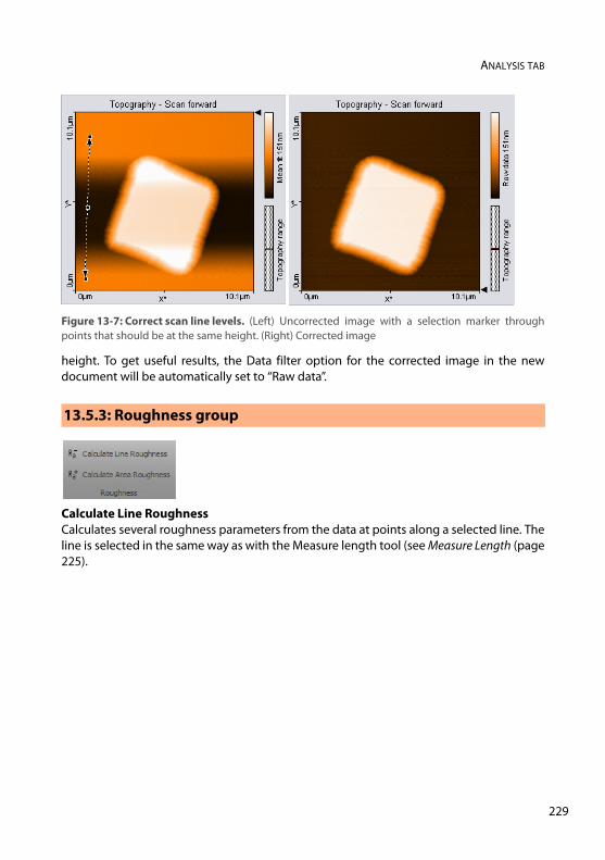
ANALYSIS TAB
height. To get useful results, the Data filter option for the corrected image in the newdocument will be automatically set to “Raw data”.
Calculate Line Roughness Calculates several roughness parameters from the data at points along a selected line. Theline is selected in the same way as with the Measure length tool (see Measure Length (page225).
Figure 13-7: Correct scan line levels. (Left) Uncorrected image with a selection marker throughpoints that should be at the same height. (Right) Corrected image
13.5.3: Roughness group
229
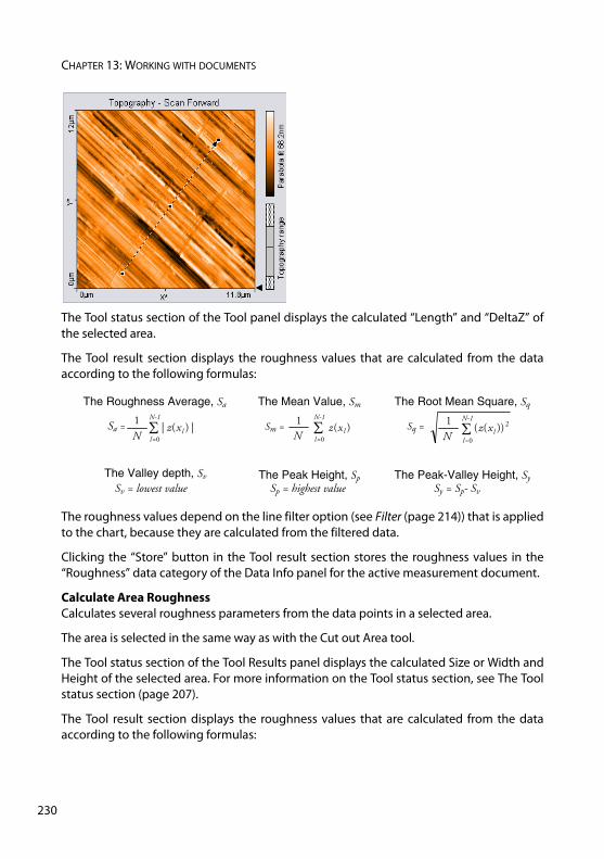
CHAPTER 13: WORKING WITH DOCUMENTS
23
The Tool status section of the Tool panel displays the calculated “Length” and “DeltaZ” ofthe selected area.
The Tool result section displays the roughness values that are calculated from the dataaccording to the following formulas:
The roughness values depend on the line filter option (see Filter (page 214)) that is appliedto the chart, because they are calculated from the filtered data.
Clicking the “Store” button in the Tool result section stores the roughness values in the“Roughness” data category of the Data Info panel for the active measurement document.
Calculate Area Roughness Calculates several roughness parameters from the data points in a selected area.
The area is selected in the same way as with the Cut out Area tool.
The Tool status section of the Tool Results panel displays the calculated Size or Width andHeight of the selected area. For more information on the Tool status section, see The Toolstatus section (page 207).
The Tool result section displays the roughness values that are calculated from the dataaccording to the following formulas:
The Roughness Average, Sa
The Valley depth, Sv
Sv = lowest value
|)(|1
0=
N-1
llxz
NSa =
The Mean Value, Sm
The Peak Height, SpSp = highest value
0=
N-1
l
)(1
lxz N
Sm =
The Root Mean Square, Sq
The Peak-Valley Height, SySy = Sp- Sv
0=
N-1
l
2))((1
lxzN
Sq =
0
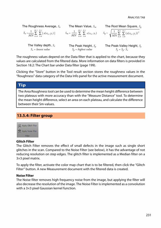
ANALYSIS TAB
The roughness values depend on the Data filter that is applied to the chart, because theyvalues are calculated from the filtered data. More information on data filters is provided inSection 18.2: The Chart bar under Data filter (page 199).
Clicking the “Store” button in the Tool result section stores the roughness values in the“Roughness” data category of the Data Info panel for the active measurement document.
Glitch FilterThe Glitch Filter removes the effect of small defects in the image such as single shortglitches in the scan. Compared to the Noise Filter (see below), it has the advantage of notreducing resolution on step edges. The glitch filter is implemented as a Median filter on a3×3 pixel matrix.
To apply the filter, activate the color map chart that is to be filtered, then click the “GlitchFilter” button. A new Measurement document with the filtered data is created.
Noise Filter The Noise filter removes high frequency noise from the image, but applying the filter willalso decrease the resolution of the image. The Noise Filter is implemented as a convolutionwith a 3×3 pixel Gaussian kernel function.
Tip The Area Roughness tool can be used to determine the mean height difference betweentwo plateaus with more accuracy than with the “Measure Distance” tool. To determinethe mean height difference, select an area on each plateau, and calculate the differencebetween their Sm-values.
13.5.4: Filter group
The Roughness Average, Sa
The Valley depth, Sv
Sv = lowest value
|),(|1
0 0= =
M-1
k
N-1
llk yxz
MNSa =
The Mean Value, Sm
The Peak Height, SpSp = highest value
0 0= =
M-1
k
N-1
l
),(1
lk yxz MN
Sm =
The Root Mean Square, Sq
The Peak-Valley Height, SySy = Sp- Sv
0 0= =
M-1
k
N-1
l
2)),((1
lk yxzMN
Sq =
231
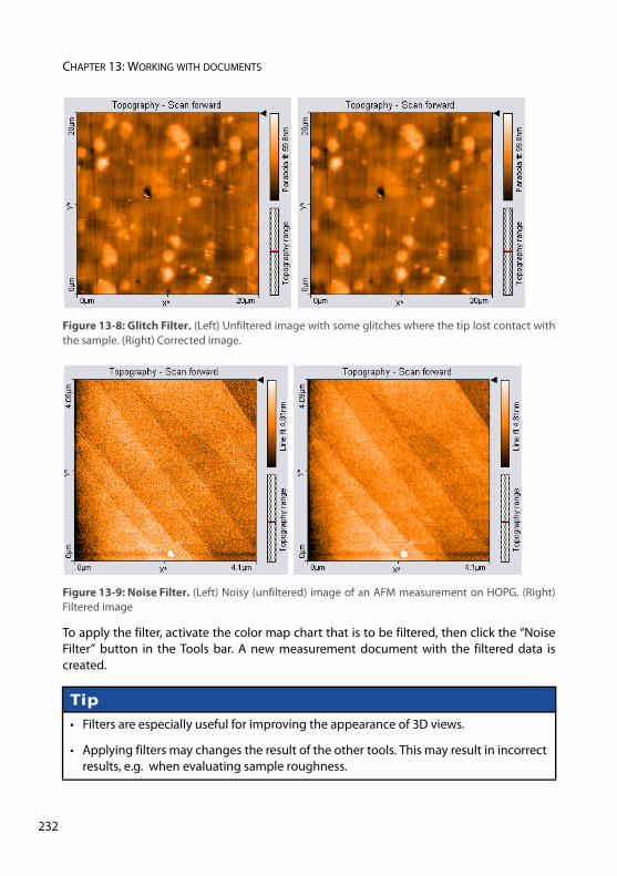
CHAPTER 13: WORKING WITH DOCUMENTS
23
To apply the filter, activate the color map chart that is to be filtered, then click the “NoiseFilter” button in the Tools bar. A new measurement document with the filtered data iscreated.
Figure 13-8: Glitch Filter. (Left) Unfiltered image with some glitches where the tip lost contact withthe sample. (Right) Corrected image.
Figure 13-9: Noise Filter. (Left) Noisy (unfiltered) image of an AFM measurement on HOPG. (Right)Filtered image
Tip• Filters are especially useful for improving the appearance of 3D views.
• Applying filters may changes the result of the other tools. This may result in incorrectresults, e.g. when evaluating sample roughness.
2
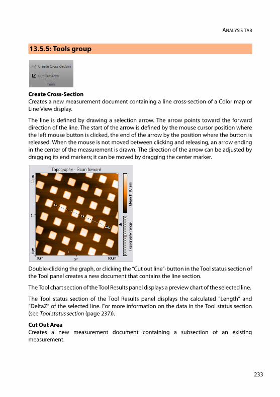
ANALYSIS TAB
Create Cross-Section Creates a new measurement document containing a line cross-section of a Color map orLine View display.
The line is defined by drawing a selection arrow. The arrow points toward the forwarddirection of the line. The start of the arrow is defined by the mouse cursor position wherethe left mouse button is clicked, the end of the arrow by the position where the button isreleased. When the mouse is not moved between clicking and releasing, an arrow endingin the center of the measurement is drawn. The direction of the arrow can be adjusted bydragging its end markers; it can be moved by dragging the center marker.
Double-clicking the graph, or clicking the “Cut out line”-button in the Tool status section ofthe Tool panel creates a new document that contains the line section.
The Tool chart section of the Tool Results panel displays a preview chart of the selected line.
The Tool status section of the Tool Results panel displays the calculated “Length” and“DeltaZ” of the selected line. For more information on the data in the Tool status section(see Tool status section (page 237)).
Cut Out Area Creates a new measurement document containing a subsection of an existingmeasurement.
13.5.5: Tools group
233
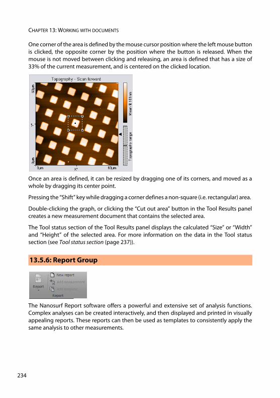
CHAPTER 13: WORKING WITH DOCUMENTS
23
One corner of the area is defined by the mouse cursor position where the left mouse buttonis clicked, the opposite corner by the position where the button is released. When themouse is not moved between clicking and releasing, an area is defined that has a size of33% of the current measurement, and is centered on the clicked location.
Once an area is defined, it can be resized by dragging one of its corners, and moved as awhole by dragging its center point.
Pressing the “Shift” key while dragging a corner defines a non-square (i.e. rectangular) area.
Double-clicking the graph, or clicking the “Cut out area” button in the Tool Results panelcreates a new measurement document that contains the selected area.
The Tool status section of the Tool Results panel displays the calculated “Size” or “Width”and “Height” of the selected area. For more information on the data in the Tool statussection (see Tool status section (page 237)).
The Nanosurf Report software offers a powerful and extensive set of analysis functions.Complex analyses can be created interactively, and then displayed and printed in visuallyappealing reports. These reports can then be used as templates to consistently apply thesame analysis to other measurements.
13.5.6: Report Group
4
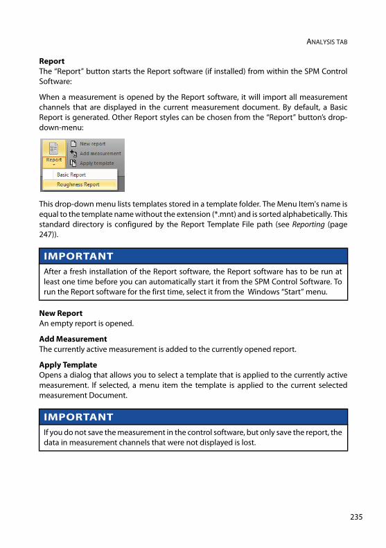
ANALYSIS TAB
ReportThe “Report” button starts the Report software (if installed) from within the SPM ControlSoftware:
When a measurement is opened by the Report software, it will import all measurementchannels that are displayed in the current measurement document. By default, a BasicReport is generated. Other Report styles can be chosen from the “Report” button’s drop-down-menu:
This drop-down menu lists templates stored in a template folder. The Menu Item's name isequal to the template name without the extension (*.mnt) and is sorted alphabetically. Thisstandard directory is configured by the Report Template File path (see Reporting (page247)).
New Report An empty report is opened.
Add Measurement The currently active measurement is added to the currently opened report.
Apply TemplateOpens a dialog that allows you to select a template that is applied to the currently activemeasurement. If selected, a menu item the template is applied to the current selectedmeasurement Document.
IMPORTANT After a fresh installation of the Report software, the Report software has to be run atleast one time before you can automatically start it from the SPM Control Software. Torun the Report software for the first time, select it from the Windows “Start” menu.
IMPORTANT If you do not save the measurement in the control software, but only save the report, thedata in measurement channels that were not displayed is lost.
235
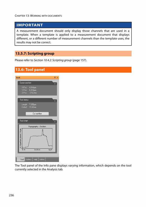
CHAPTER 13: WORKING WITH DOCUMENTS
23
Please refer to Section 10.4.2: Scripting group (page 157).
The Tool panel of the Info pane displays varying information, which depends on the toolcurrently selected in the Analysis tab.
A measurement document should only display those channels that are used in atemplate. When a template is applied to a measurement document that displaysdifferent, or a different number of measurement channels than the template uses, theresults may not be correct.
13.5.7: Scripting group
13.6: Tool panel
IMPORTANT
6
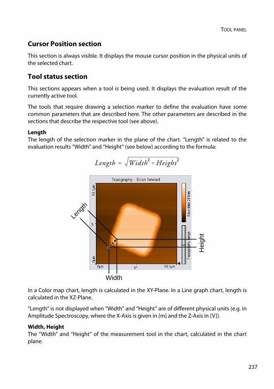
TOOL PANEL
Cursor Position section
This section is always visible. It displays the mouse cursor position in the physical units ofthe selected chart.
Tool status section
This sections appears when a tool is being used. It displays the evaluation result of thecurrently active tool.
The tools that require drawing a selection marker to define the evaluation have somecommon parameters that are described here. The other parameters are described in thesections that describe the respective tool (see above).
Length The length of the selection marker in the plane of the chart. “Length” is related to theevaluation results “Width” and “Height” (see below) according to the formula:
In a Color map chart, length is calculated in the XY-Plane. In a Line graph chart, length iscalculated in the XZ-Plane.
“Length” is not displayed when “Width” and “Height” are of different physical units (e.g. inAmplitude Spectroscopy, where the X-Axis is given in [m] and the Z-Axis in [V]).
Width, Height The “Width” and “Height” of the measurement tool in the chart, calculated in the chartplane.
Length Width2 Height2+=
Width
Hei
ght
Leng
th
237
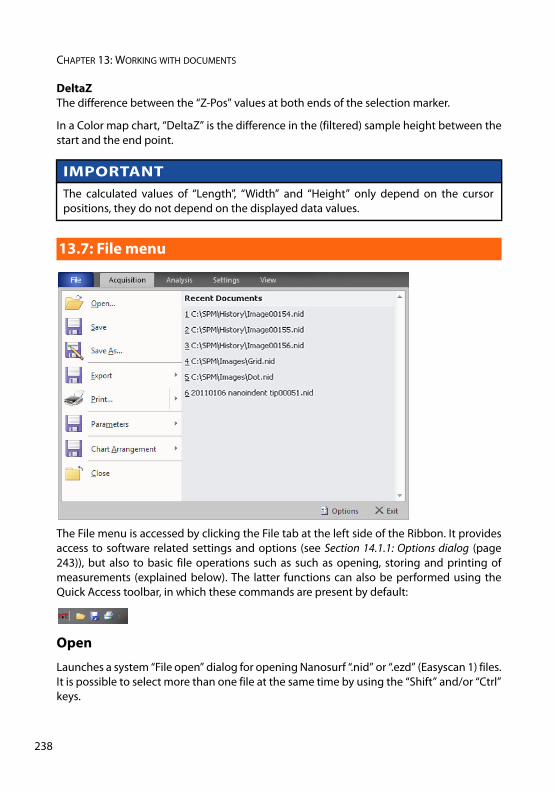
CHAPTER 13: WORKING WITH DOCUMENTS
23
DeltaZ The difference between the “Z-Pos” values at both ends of the selection marker.
In a Color map chart, “DeltaZ” is the difference in the (filtered) sample height between thestart and the end point.
The File menu is accessed by clicking the File tab at the left side of the Ribbon. It providesaccess to software related settings and options (see Section 14.1.1: Options dialog (page243)), but also to basic file operations such as such as opening, storing and printing ofmeasurements (explained below). The latter functions can also be performed using theQuick Access toolbar, in which these commands are present by default:
Open
Launches a system “File open” dialog for opening Nanosurf “.nid” or “.ezd” (Easyscan 1) files.It is possible to select more than one file at the same time by using the “Shift” and/or “Ctrl”keys.
IMPORTANT The calculated values of “Length”, “Width” and “Height” only depend on the cursorpositions, they do not depend on the displayed data values.
13.7: File menu
8
FILE MENU
Selected files will open in document windows, which contains a chart area and a data infopanel. There is no Imaging toolbar like there is for ongoing measurements in the Imagingwindow. You can however still customize the charts through a context menu, which opensthrough a right-click. The data info Panel displays all significant parameters were used forthe measurement. For more information on Measurement document functionality, seeSection 13.1: Introduction.
Save / Save as...
Save a measurement document in Nanosurf image data format (file extension “.nid”). Thesame dialog is opened for both menu items.
Close
Closes the currently active document, but not the SPM control software. If you haveunsaved data in the current document, you will be asked to save it.
Export
Exports either the active chart or the whole active measurement document for use in otherprograms or image-processing software. Available data types for documents are taggedimage file format (.tif ), portable network graphics (.png), Windows bitmap (.bmp), 16 bitdata file (.dat), and plot file (.plt). For Charts, additional available data types are commaseparated z values (.csv), and (X,Y,Z)points (.csv).
When the data is exported using the function “Export” >> “Current document as...”, everyChart in the measurement document is stored in the export file consecutively. In the binaryformat, the blocks of data from each Chart are stored directly one behind the other. In the“ASCII” text format the blocks of data for each Chart are separated by two empty lines.
Tagged image file format (.tif), portable network graphics (.png), and Windowsbitmap (.bmp) All of these image file formats are suitable for inclusion of images in electronic documents,e.g. in Word, PowerPoint or image-processing software. The exact image as seen on thecomputer screen will be saved in the exported file (similar to a screenshot of the respectivechart).
Data file 16Bit (.dat) A binary data file that can be processed in data processing software. This “binary” dataformat only contains the measured data. The data is stored consecutively, line by lineupwards, as 16-bit values (–32768 to +32767). Before being stored, the data is processedusing the settings chosen in the Correction and Filter groups of the Analysis tab (see Section13.5: Analysis tab for details).
239
CHAPTER 13: WORKING WITH DOCUMENTS
24
Plotfile ASCII (.plt) This is an “ASCII” text format which contains the measured data as well as a small headerwith a description of the scan. A plotfile can be used for detailed data analysis by variousmathematical software packages such as MathLab, or for plotting by software such asGnuPlot. Before being stored, the data is processed using the settings chosen in theCorrection and Filter groups of the Analysis tab (see Section 13.5: Analysis tab for details).
If “Line graph” is selected as “Display” in the “Chart bar”, only the visualized lines will bestored. Each data point is stored as a pair of floating point numbers on a separate line. Thenumber pairs are separated by a blank character (SPACE).
If any other chart type is selected, all measured values are stored. All values in a data lineare stored on a separate line in the text file. An empty line is inserted after every data line.The data lines are stored from the bottom to the top. A small header at the beginning of thefirst data line contains the names of the channel and frame, as well as X-, Y-, and Z-rangeswith their physical units.
Comma separated z values (.csv) This format stores all the measured data in a chart, as a matrix of floating point numbers inASCII format separated by a “comma” and “SPACE” character. This enables easy dataexchange with commonly used spread sheet and database applications.
(X, Y, Z)-Points (.csv) This format stores the coordinates of all measured points in a chart as a list of floating pointnumber pairs. For Line graphs, only X and Z points are exported.
Print / Print preview...
Prints the currently selected measurement document together with the values shown inthe Data Info panel.
Exit
With exit you can close the SPM Control Software. If you exit the program while still havingunsaved data, you will be asked to save it.
0

CHAPTER 14:
Options and settings0
0
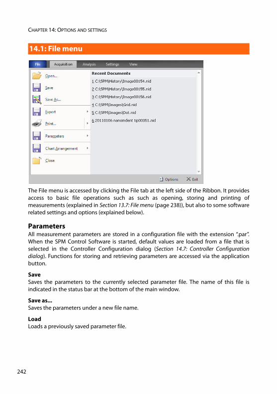
CHAPTER 14: OPTIONS AND SETTINGS
24
The File menu is accessed by clicking the File tab at the left side of the Ribbon. It providesaccess to basic file operations such as such as opening, storing and printing ofmeasurements (explained in Section 13.7: File menu (page 238)), but also to some softwarerelated settings and options (explained below).
ParametersAll measurement parameters are stored in a configuration file with the extension “.par”.When the SPM Control Software is started, default values are loaded from a file that isselected in the Controller Configuration dialog (Section 14.7: Controller Configurationdialog). Functions for storing and retrieving parameters are accessed via the applicationbutton.
SaveSaves the parameters to the currently selected parameter file. The name of this file isindicated in the status bar at the bottom of the main window.
Save as...Saves the parameters under a new file name.
LoadLoads a previously saved parameter file.
14.1: File menu
2
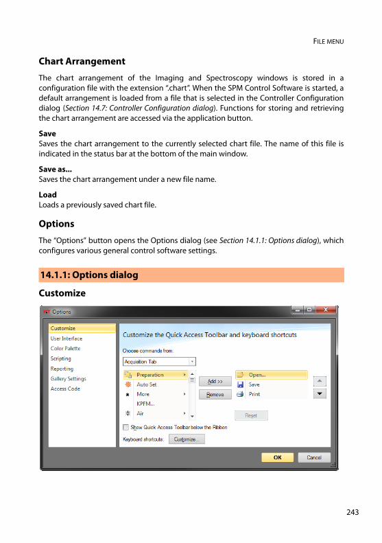
FILE MENU
Chart Arrangement
The chart arrangement of the Imaging and Spectroscopy windows is stored in aconfiguration file with the extension “.chart”. When the SPM Control Software is started, adefault arrangement is loaded from a file that is selected in the Controller Configurationdialog (Section 14.7: Controller Configuration dialog). Functions for storing and retrievingthe chart arrangement are accessed via the application button.
SaveSaves the chart arrangement to the currently selected chart file. The name of this file isindicated in the status bar at the bottom of the main window.
Save as...Saves the chart arrangement under a new file name.
LoadLoads a previously saved chart file.
Options
The “Options” button opens the Options dialog (see Section 14.1.1: Options dialog), whichconfigures various general control software settings.
Customize
14.1.1: Options dialog
243
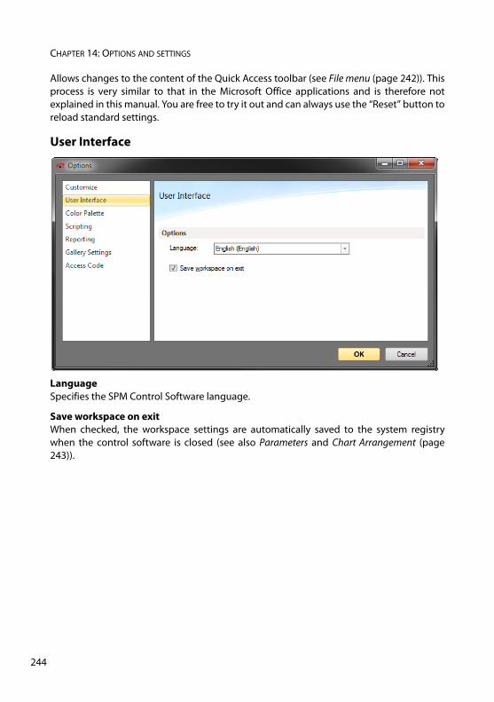
CHAPTER 14: OPTIONS AND SETTINGS
24
Allows changes to the content of the Quick Access toolbar (see File menu (page 242)). Thisprocess is very similar to that in the Microsoft Office applications and is therefore notexplained in this manual. You are free to try it out and can always use the “Reset” button toreload standard settings.
User Interface
LanguageSpecifies the SPM Control Software language.
Save workspace on exitWhen checked, the workspace settings are automatically saved to the system registrywhen the control software is closed (see also Parameters and Chart Arrangement (page243)).
4
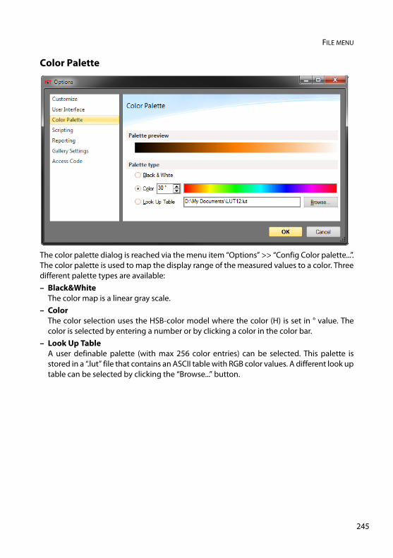
FILE MENU
Color Palette
The color palette dialog is reached via the menu item “Options” >> “Config Color palette...”.The color palette is used to map the display range of the measured values to a color. Threedifferent palette types are available: – Black&White
The color map is a linear gray scale.– Color
The color selection uses the HSB-color model where the color (H) is set in ° value. Thecolor is selected by entering a number or by clicking a color in the color bar.
– Look Up TableA user definable palette (with max 256 color entries) can be selected. This palette isstored in a “.lut” file that contains an ASCII table with RGB color values. A different look uptable can be selected by clicking the “Browse...” button.
245
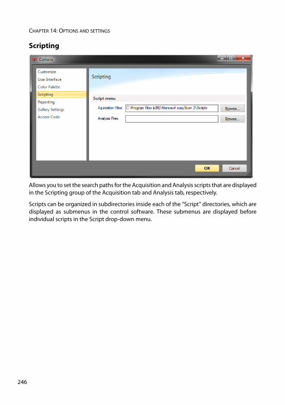
CHAPTER 14: OPTIONS AND SETTINGS
24
Scripting
Allows you to set the search paths for the Acquisition and Analysis scripts that are displayedin the Scripting group of the Acquisition tab and Analysis tab, respectively.
Scripts can be organized in subdirectories inside each of the “Script” directories, which aredisplayed as submenus in the control software. These submenus are displayed beforeindividual scripts in the Script drop-down menu.
6
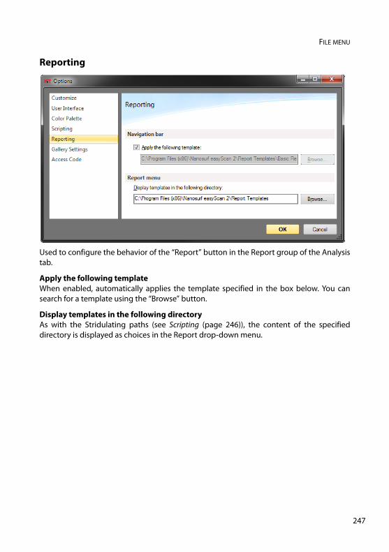
FILE MENU
Reporting
Used to configure the behavior of the “Report” button in the Report group of the Analysistab.
Apply the following templateWhen enabled, automatically applies the template specified in the box below. You cansearch for a template using the “Browse” button.
Display templates in the following directoryAs with the Stridulating paths (see Scripting (page 246)), the content of the specifieddirectory is displayed as choices in the Report drop-down menu.
247
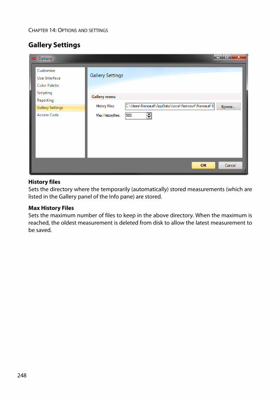
CHAPTER 14: OPTIONS AND SETTINGS
24
Gallery Settings
History filesSets the directory where the temporarily (automatically) stored measurements (which arelisted in the Gallery panel of the Info pane) are stored.
Max History FilesSets the maximum number of files to keep in the above directory. When the maximum isreached, the oldest measurement is deleted from disk to allow the latest measurement tobe saved.
8
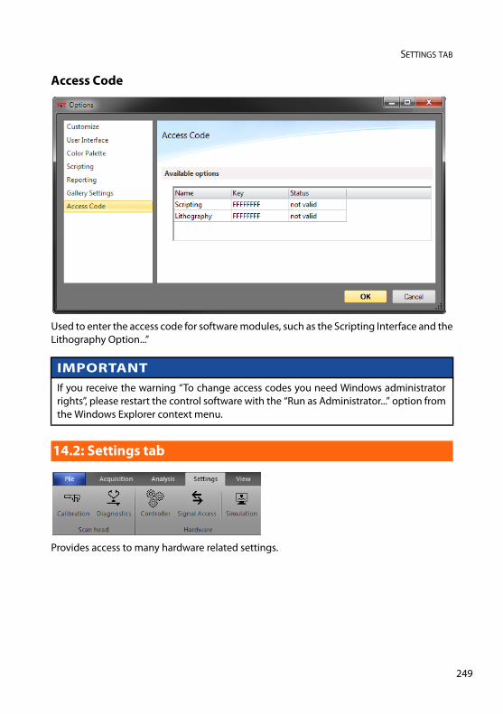
SETTINGS TAB
Access Code
Used to enter the access code for software modules, such as the Scripting Interface and theLithography Option...”
Provides access to many hardware related settings.
IMPORTANTIf you receive the warning “To change access codes you need Windows administratorrights”, please restart the control software with the “Run as Administrator...” option fromthe Windows Explorer context menu.
14.2: Settings tab
249
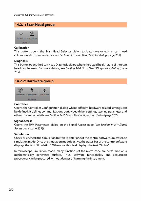
CHAPTER 14: OPTIONS AND SETTINGS
25
Calibration This button opens the Scan Head Selector dialog to load, save or edit a scan headcalibration file. For more details, see Section 14.3: Scan Head Selector dialog (page 251).
DiagnosisThis button opens the Scan Head Diagnosis dialog where the actual health state of the scanhead can be seen. For more details, see Section 14.6: Scan Head Diagnostics dialog (page255).
ControllerOpens the Controller Configuration dialog where different hardware related settings canbe defined. It defines communications port, video driver settings, start up parameter andothers. For more details, see Section 14.7: Controller Configuration dialog (page 257).
Signal AccessOpens the SPM Parameters dialog on the Signal Access page (see Section 14.8.1: SignalAccess page (page 259)).
SimulationCheck or uncheck the Simulation button to enter or exit the control software’s microscopesimulation mode. Once the simulation mode is active, the status bar of the control softwaredisplays the text “Simulation”. Otherwise, this field displays the text “Online”.
In microscope simulation mode, many functions of the microscope are performed on amathematically generated surface. Thus, software functionality and acquisitionprocedures can be practised without danger of harming the instrument.
14.2.1: Scan Head group
14.2.2: Hardware group
0
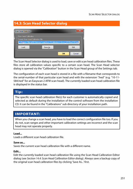
SCAN HEAD SELECTOR DIALOG
The Scan Head Selector dialog is used to load, save or edit scan head calibration files. Thesefiles store all calibration values specific to a certain scan head. The Scan Head selectordialog is opened via the “Calibration” button in the Scan Head group of the Settings tab.
The configuration of each scan head is stored in a file with a filename that corresponds tothe serial-number of that particular scan head and with the extension “.hed” (e.g. “10-11-584.hed” for an Easyscan 2 AFM scan head). The currently loaded scan head calibration fileis displayed in the status bar.
Load... Loads a different scan head calibration file.
Save as... Saves the current scan head calibration file with a different name.
Edit... Edit the currently loaded scan head calibration file using the Scan Head Calibration Editordialog (see Section 14.4: Scan Head Calibration Editor dialog). Always save a backup copy ofthe original scan head calibration files by clicking 'Save As...' first.
14.3: Scan Head Selector dialog
Tip:The specific scan head calibration file(s) for each customer is automatically copied andselected as default during the installation of the control software from the installationCD. It can be found in the “Calibrations” sub directory of your installation path.
IMPORTANT:When you change a scan head, you have to load the correct configuration file too. If youdo not, scan ranges and other important calibration settings are incorrect and the scanhead may not operate properly.
251
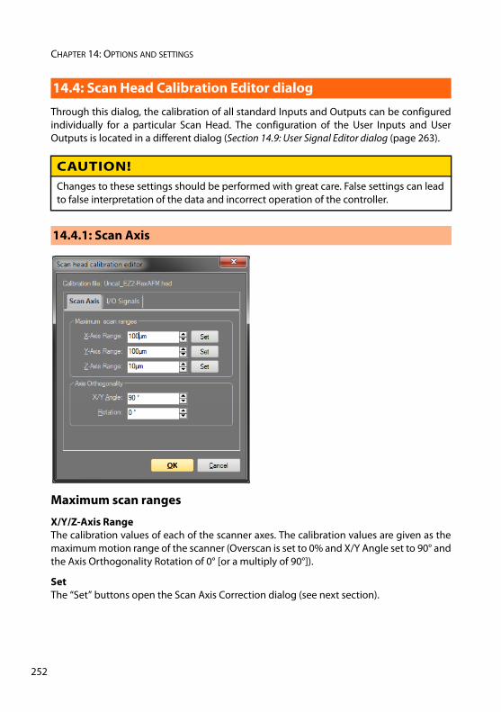
CHAPTER 14: OPTIONS AND SETTINGS
25
Through this dialog, the calibration of all standard Inputs and Outputs can be configuredindividually for a particular Scan Head. The configuration of the User Inputs and UserOutputs is located in a different dialog (Section 14.9: User Signal Editor dialog (page 263).
Maximum scan ranges
X/Y/Z-Axis Range The calibration values of each of the scanner axes. The calibration values are given as themaximum motion range of the scanner (Overscan is set to 0% and X/Y Angle set to 90° andthe Axis Orthogonality Rotation of 0° [or a multiply of 90°]).
Set The “Set” buttons open the Scan Axis Correction dialog (see next section).
14.4: Scan Head Calibration Editor dialog
CAUTION!Changes to these settings should be performed with great care. False settings can leadto false interpretation of the data and incorrect operation of the controller.
14.4.1: Scan Axis
2
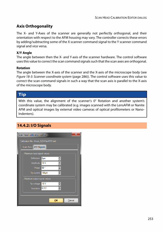
SCAN HEAD CALIBRATION EDITOR DIALOG
Axis Orthogonality
The X- and Y-Axes of the scanner are generally not perfectly orthogonal, and theirorientation with respect to the AFM housing may vary. The controller corrects these errorsby adding/subtracting some of the X scanner command signal to the Y scanner commandsignal and vice versa.
X/Y Angle The angle between then the X- and Y-axis of the scanner hardware. The control softwareuses this value to correct the scan command signals such that the scan axes are orthogonal.
Rotation The angle between the X-axis of the scanner and the X-axis of the microscope body (seeFigure 18-3: Scanner coordinate system (page 286)). The control software uses this value tocorrect the scan command signals in such a way that the scan axis is parallel to the X-axisof the microscope body.
TipWith this value, the alignment of the scanner's 0° Rotation and another system’scoordinate system may be calibrated (e.g. images scanned with the LensAFM or NaniteAFM and optical images by external video cameras of optical profilometers or Nano-Indenters).
14.4.2: I/O Signals
253
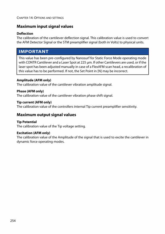
CHAPTER 14: OPTIONS AND SETTINGS
25
Maximum input signal values
Deflection The calibration of the cantilever deflection signal. This calibration value is used to convertthe AFM Detector Signal or the STM preamplifier signal (both in Volts) to physical units.
Amplitude (AFM only)The calibration value of the cantilever vibration amplitude signal.
Phase (AFM only)The calibration value of the cantilever vibration phase shift signal.
Tip current (AFM only)The calibration value of the controllers internal Tip current preamplifier sensitivity.
Maximum output signal values
Tip Potential The calibration value of the Tip voltage setting.
Excitation (AFM only)The calibration value of the Amplitude of the signal that is used to excite the cantilever indynamic force operating modes.
IMPORTANTThis value has been pre-configured by Nanosurf for Static Force Mode operating modewith CONTR Cantilever and a Laser Spot at 225 μm. If other Cantilevers are used, or if thelaser spot has been adjusted manually in case of a FlexAFM scan head, a recalibration ofthis value has to be performed. If not, the Set Point in [N] may be incorrect.
4
SCAN AXIS CORRECTION DIALOG
This dialog can be used to correct the scan range by entering a correction factor based ona measured distance and a known real distance.
This correction factor could for example be determined by evaluating the heightinformation in a measurement of a calibration grid with known properties.
Scan axis correction
Correction coefficientThe scan range is multiplied with this number when the “Set” button is clicked.
The Scan Head Diagnostics dialog displays the current status of the scan head. It is openedby clicking the “Diagnostics” button in Scan Head group of the Settings tab.
14.5: Scan Axis Correction dialog
14.6: Scan Head Diagnostics dialog
TipThe Scan Head Diagnostics dialog cannot be accessed once the tip has beenapproached to the sample. In this case, retract the tip first.
255
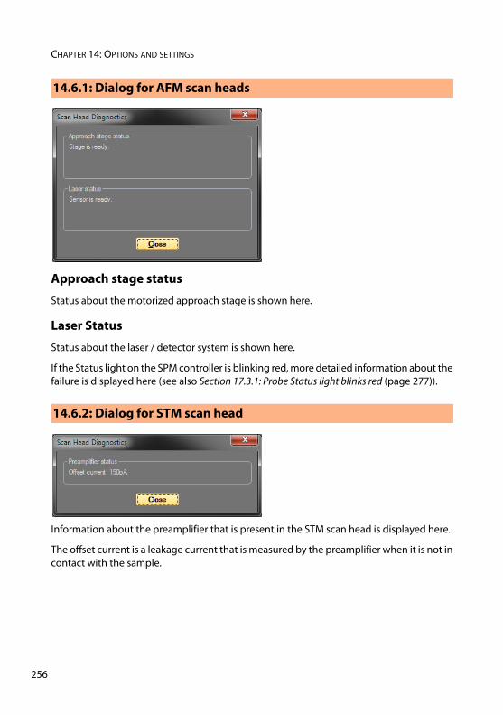
CHAPTER 14: OPTIONS AND SETTINGS
25
Approach stage status
Status about the motorized approach stage is shown here.
Laser Status
Status about the laser / detector system is shown here.
If the Status light on the SPM controller is blinking red, more detailed information about thefailure is displayed here (see also Section 17.3.1: Probe Status light blinks red (page 277)).
Information about the preamplifier that is present in the STM scan head is displayed here.
The offset current is a leakage current that is measured by the preamplifier when it is not incontact with the sample.
14.6.1: Dialog for AFM scan heads
14.6.2: Dialog for STM scan head
6
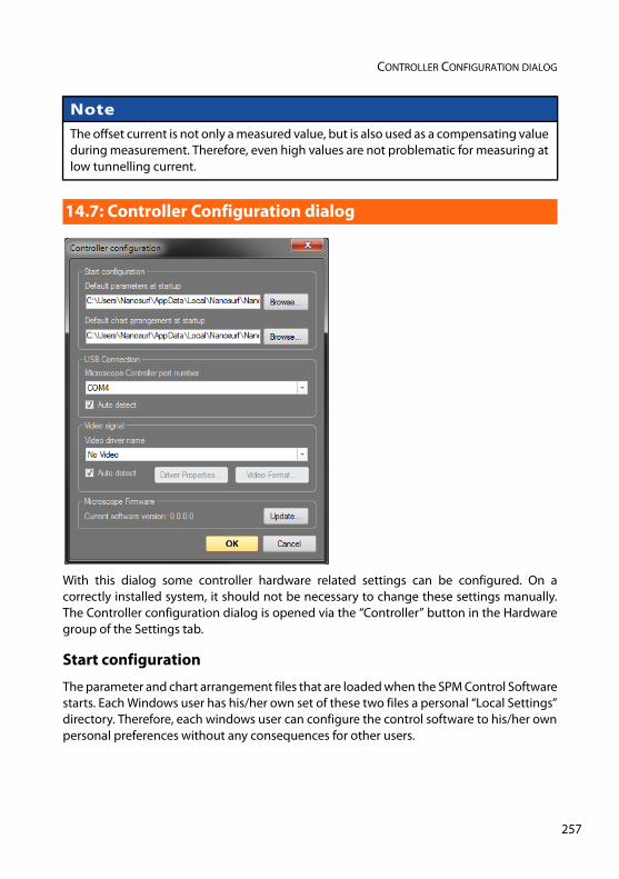
CONTROLLER CONFIGURATION DIALOG
?
With this dialog some controller hardware related settings can be configured. On acorrectly installed system, it should not be necessary to change these settings manually.The Controller configuration dialog is opened via the “Controller” button in the Hardwaregroup of the Settings tab.
Start configuration
The parameter and chart arrangement files that are loaded when the SPM Control Softwarestarts. Each Windows user has his/her own set of these two files a personal “Local Settings”directory. Therefore, each windows user can configure the control software to his/her ownpersonal preferences without any consequences for other users.
NoteThe offset current is not only a measured value, but is also used as a compensating valueduring measurement. Therefore, even high values are not problematic for measuring atlow tunnelling current.
14.7: Controller Configuration dialog
257
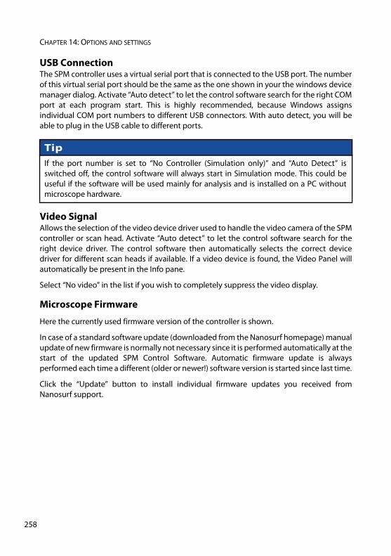
CHAPTER 14: OPTIONS AND SETTINGS
25
USB Connection The SPM controller uses a virtual serial port that is connected to the USB port. The numberof this virtual serial port should be the same as the one shown in your the windows devicemanager dialog. Activate “Auto detect” to let the control software search for the right COMport at each program start. This is highly recommended, because Windows assignsindividual COM port numbers to different USB connectors. With auto detect, you will beable to plug in the USB cable to different ports.
Video Signal Allows the selection of the video device driver used to handle the video camera of the SPMcontroller or scan head. Activate “Auto detect” to let the control software search for theright device driver. The control software then automatically selects the correct devicedriver for different scan heads if available. If a video device is found, the Video Panel willautomatically be present in the Info pane.
Select “No video” in the list if you wish to completely suppress the video display.
Microscope Firmware
Here the currently used firmware version of the controller is shown.
In case of a standard software update (downloaded from the Nanosurf homepage) manualupdate of new firmware is normally not necessary since it is performed automatically at thestart of the updated SPM Control Software. Automatic firmware update is alwaysperformed each time a different (older or newer!) software version is started since last time.
Click the “Update” button to install individual firmware updates you received fromNanosurf support.
TipIf the port number is set to “No Controller (Simulation only)” and “Auto Detect” isswitched off, the control software will always start in Simulation mode. This could beuseful if the software will be used mainly for analysis and is installed on a PC withoutmicroscope hardware.
8
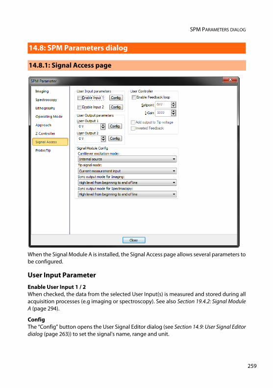
SPM PARAMETERS DIALOG
When the Signal Module A is installed, the Signal Access page allows several parameters tobe configured.
User Input Parameter
Enable User Input 1 / 2 When checked, the data from the selected User Input(s) is measured and stored during allacquisition processes (e.g imaging or spectroscopy). See also Section 19.4.2: Signal ModuleA (page 294).
ConfigThe “Config” button opens the User Signal Editor dialog (see Section 14.9: User Signal Editordialog (page 263)) to set the signal's name, range and unit.
14.8: SPM Parameters dialog
14.8.1: Signal Access page
259
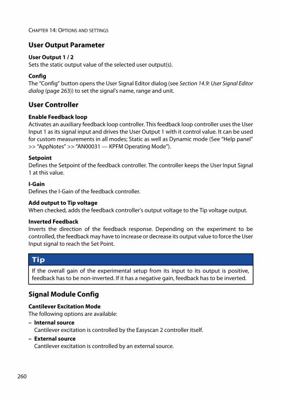
CHAPTER 14: OPTIONS AND SETTINGS
26
User Output Parameter
User Output 1 / 2 Sets the static output value of the selected user output(s).
ConfigThe “Config” button opens the User Signal Editor dialog (see Section 14.9: User Signal Editordialog (page 263)) to set the signal's name, range and unit.
User Controller
Enable Feedback loop Activates an auxiliary feedback loop controller. This feedback loop controller uses the UserInput 1 as its signal input and drives the User Output 1 with it control value. It can be usedfor custom measurements in all modes; Static as well as Dynamic mode (See “Help panel”>> “AppNotes” >> “AN00031 — KPFM Operating Mode”).
Setpoint Defines the Setpoint of the feedback controller. The controller keeps the User Input Signal1 at this value.
I-Gain Defines the I-Gain of the feedback controller.
Add output to Tip voltage When checked, adds the feedback controller's output voltage to the Tip voltage output.
Inverted Feedback Inverts the direction of the feedback response. Depending on the experiment to becontrolled, the feedback may have to increase or decrease its output value to force the UserInput signal to reach the Set Point.
Signal Module Config
Cantilever Excitation Mode The following options are available: – Internal source
Cantilever excitation is controlled by the Easyscan 2 controller itself. – External source
Cantilever excitation is controlled by an external source.
TipIf the overall gain of the experimental setup from its input to its output is positive,feedback has to be non-inverted. If it has a negative gain, feedback has to be inverted.
0
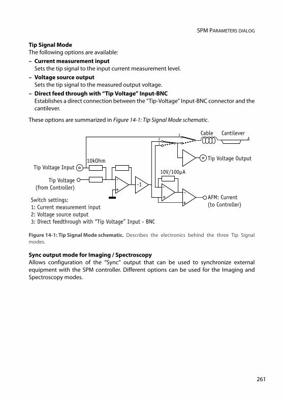
SPM PARAMETERS DIALOG
Tip Signal Mode The following options are available:– Current measurement input
Sets the tip signal to the input current measurement level. – Voltage source output
Sets the tip signal to the measured output voltage. – Direct feed through with “Tip Voltage” Input-BNC
Establishes a direct connection between the “Tip-Voltage” Input-BNC connector and thecantilever.
These options are summarized in Figure 14-1: Tip Signal Mode schematic.
Sync output mode for Imaging / SpectroscopyAllows configuration of the “Sync” output that can be used to synchronize externalequipment with the SPM controller. Different options can be used for the Imaging andSpectroscopy modes.
Figure 14-1: Tip Signal Mode schematic. Describes the electronics behind the three Tip Signalmodes.
Tip Voltage(from Controller)
Tip Voltage Input
-
+
10kOhm
10V/100µA
AFM: Current (to Controller)
-
+
-
+
-1
Cable Cantilever
12
Tip Voltage Output
3
Switch settings:1: Current measurement input2: Voltage source output3: Direct feedthrough with “Tip Voltage” Input - BNC
261
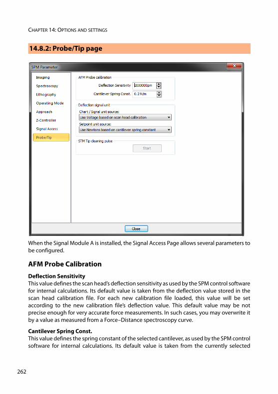
CHAPTER 14: OPTIONS AND SETTINGS
26
When the Signal Module A is installed, the Signal Access Page allows several parameters tobe configured.
AFM Probe Calibration
Deflection SensitivityThis value defines the scan head’s deflection sensitivity as used by the SPM control softwarefor internal calculations. Its default value is taken from the deflection value stored in thescan head calibration file. For each new calibration file loaded, this value will be setaccording to the new calibration file’s deflection value. This default value may be notprecise enough for very accurate force measurements. In such cases, you may overwrite itby a value as measured from a Force–Distance spectroscopy curve.
Cantilever Spring Const.This value defines the spring constant of the selected cantilever, as used by the SPM controlsoftware for internal calculations. Its default value is taken from the currently selected
14.8.2: Probe/Tip page
2
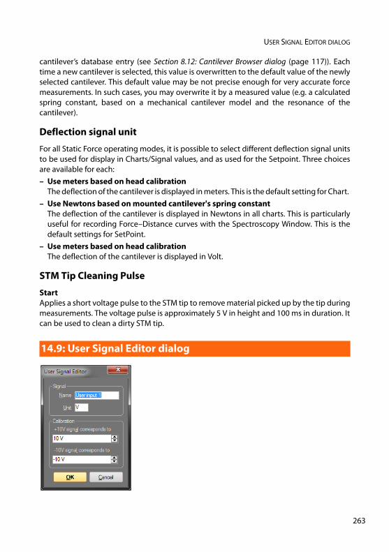
USER SIGNAL EDITOR DIALOG
cantilever’s database entry (see Section 8.12: Cantilever Browser dialog (page 117)). Eachtime a new cantilever is selected, this value is overwritten to the default value of the newlyselected cantilever. This default value may be not precise enough for very accurate forcemeasurements. In such cases, you may overwrite it by a measured value (e.g. a calculatedspring constant, based on a mechanical cantilever model and the resonance of thecantilever).
Deflection signal unit
For all Static Force operating modes, it is possible to select different deflection signal unitsto be used for display in Charts/Signal values, and as used for the Setpoint. Three choicesare available for each: – Use meters based on head calibration
The deflection of the cantilever is displayed in meters. This is the default setting for Chart. – Use Newtons based on mounted cantilever's spring constant
The deflection of the cantilever is displayed in Newtons in all charts. This is particularlyuseful for recording Force–Distance curves with the Spectroscopy Window. This is thedefault settings for SetPoint.
– Use meters based on head calibrationThe deflection of the cantilever is displayed in Volt.
STM Tip Cleaning Pulse
StartApplies a short voltage pulse to the STM tip to remove material picked up by the tip duringmeasurements. The voltage pulse is approximately 5 V in height and 100 ms in duration. Itcan be used to clean a dirty STM tip.
14.9: User Signal Editor dialog
263

CHAPTER 14: OPTIONS AND SETTINGS
26
The User Signal Editor dialog is used for editing the calibration of the User Input/Outputsignals. The settings made in this dialog are stored in the active Scan Head calibration file.
Name The name of the user signal. The entered name is used throughout the control software.
Unit The base unit of the physical signal, without prefix (i.e. ‘m’, not ‘nm’ or ‘μm’).
Calibration The physical signal values that correspond to the maximum and minimum signal voltagesshould be entered here. Prefixes can be used.
4

CHAPTER 15:
Quick reference
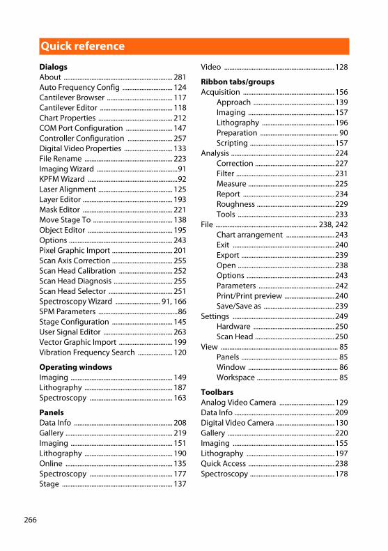
26
DialogsAbout ............................................................... 281Auto Frequency Config ............................. 124Cantilever Browser ...................................... 117Cantilever Editor .......................................... 118Chart Properties ........................................... 212COM Port Configuration ........................... 147Controller Configuration .......................... 257Digital Video Properties ............................ 133File Rename ................................................... 223Imaging Wizard ...............................................91KPFM Wizard ....................................................92Laser Alignment ........................................... 125Layer Editor .................................................... 193Mask Editor .................................................... 221Move Stage To .............................................. 138Object Editor ................................................. 195Options ............................................................ 243Pixel Graphic Import ................................... 201Scan Axis Correction ................................... 255Scan Head Calibration ............................... 252Scan Head Diagnosis .................................. 255Scan Head Selector ..................................... 251Spectroscopy Wizard .......................... 91, 166SPM Parameters ..............................................86Stage Configuration ................................... 145User Signal Editor ........................................ 263Vector Graphic Import ............................... 199Vibration Frequency Search .................... 120
Operating windowsImaging ........................................................... 149Lithography ................................................... 187Spectroscopy ................................................ 163
PanelsData Info ......................................................... 208Gallery .............................................................. 219Imaging ........................................................... 151Lithography ................................................... 190Online .............................................................. 135Spectroscopy ................................................ 177Stage ................................................................ 137
Video ................................................................128
Ribbon tabs/groupsAcquisition .....................................................156
Approach ...............................................139Imaging ..................................................157Lithography ..........................................196Preparation ............................................. 90Scripting .................................................157
Analysis ............................................................224Correction ..............................................227Filter .........................................................231Measure ..................................................225Report .....................................................234Roughness .............................................229Tools ........................................................233
File ........................................................... 238, 242Chart arrangement ............................243Exit ...........................................................240Export ......................................................239Open ........................................................238Options ...................................................243Parameters ............................................242Print/Print preview .............................240Save/Save as .........................................239
Settings ...........................................................249Hardware ...............................................250Scan Head ..............................................250
View .................................................................... 85Panels ........................................................ 85Window .................................................... 86Workspace ............................................... 85
ToolbarsAnalog Video Camera ................................129Data Info ..........................................................209Digital Video Camera ..................................130Gallery ..............................................................220Imaging ...........................................................155Lithography ...................................................197Quick Access ..................................................238Spectroscopy .................................................178
Quick reference
6

PART C:
APPENDICES


CHAPTER 16:
Maintenance0
0

CHAPTER 16: MAINTENANCE
27
To ensure fault-free operation of the microscope, the maintenance instructions below haveto be observed.
It is important to keep the open parts of the scan head clean. Therefore, always store thescan head in a dust-free and dry environment when it is not in use. If exposed to moisture(high humidity) over a prolonged period, corrosion will occur.
The cantilever holder should be cleaned after each use in liquid environment. If it shouldstill become dirty over time, use the following procedure to clean it:
1 Use a mild dish soap to clean the cantilever chip and SureAlign optics on the outsideof the cantilever holder. Avoid wetting the inside of the cantilever holder, unless the optical components aredirty on the inside as well. In this case:A Use a slightly wettened cotton bud to clean dirty parts on the inside of the
cantilever holder.B Use a fresh cotton bud to dry the clean surfaces.A cotton bud may be used on the outside of the cantilever holder as well to assist inremoving sticky residues.
2 Wash the outside of the cantilever holder with water.
3 Wash the outside of the cantilever holder with 70% ethanol or 100% iso-propanol(sometimes written as 2-propanol).Both solvents can remove most non-water-soluble residues, such as the onesdeposited by air dusters (if these are not used properly). The 70% ethanol treatment isalso a good way to sterilize the cantilever holder when it has been used with liquidsand biological samples (e.g. living microorganisms).
4 Air-dry the cantilever holder and store it dust-free.
To clean the case and the controls of the controller:
16.1: Introduction
16.2: The FlexAFM scan head
16.3: The cantilever holder
16.4: The Easyscan 2 controller
0

THE EASYSCAN 2 CONTROLLER
> Use a soft cloth, lightly moistened with a mild detergent solution. Do not use anyabrasive pads or solvents like alcohol or spirits.
271

CHAPTER 16: MAINTENANCE
27
2
CHAPTER 17:
Problems and solutions0
0
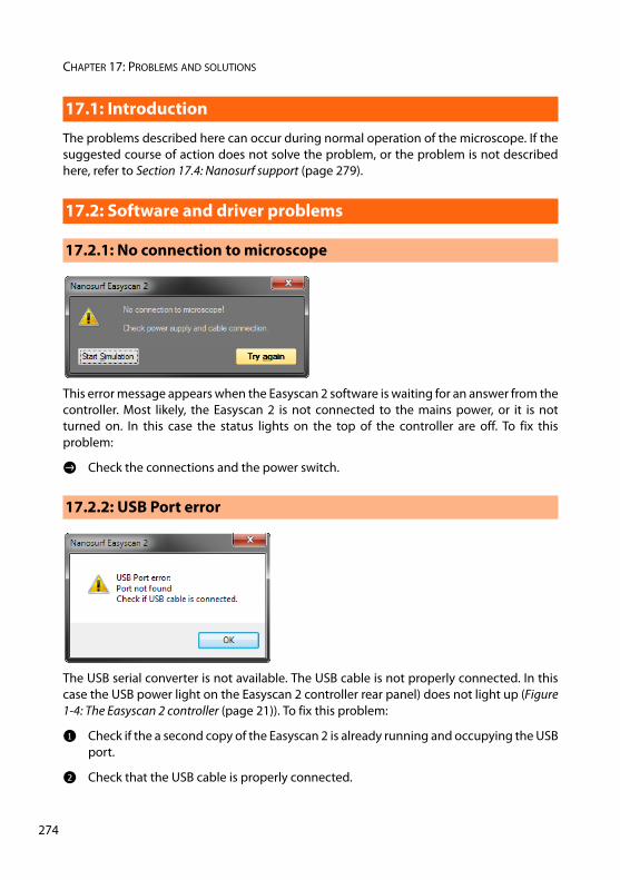
CHAPTER 17: PROBLEMS AND SOLUTIONS
27
The problems described here can occur during normal operation of the microscope. If thesuggested course of action does not solve the problem, or the problem is not describedhere, refer to Section 17.4: Nanosurf support (page 279).
This error message appears when the Easyscan 2 software is waiting for an answer from thecontroller. Most likely, the Easyscan 2 is not connected to the mains power, or it is notturned on. In this case the status lights on the top of the controller are off. To fix thisproblem:
> Check the connections and the power switch.
The USB serial converter is not available. The USB cable is not properly connected. In thiscase the USB power light on the Easyscan 2 controller rear panel) does not light up (Figure1-4: The Easyscan 2 controller (page 21)). To fix this problem:
1 Check if the a second copy of the Easyscan 2 is already running and occupying the USBport.
2 Check that the USB cable is properly connected.
17.1: Introduction
17.2: Software and driver problems
17.2.1: No connection to microscope
17.2.2: USB Port error
4
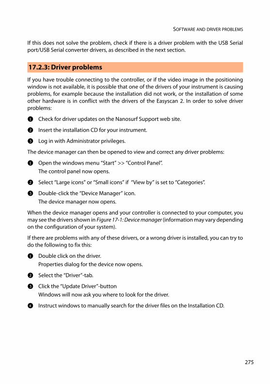
SOFTWARE AND DRIVER PROBLEMS
If this does not solve the problem, check if there is a driver problem with the USB Serialport/USB Serial converter drivers, as described in the next section.
If you have trouble connecting to the controller, or if the video image in the positioningwindow is not available, it is possible that one of the drivers of your instrument is causingproblems, for example because the installation did not work, or the installation of someother hardware is in conflict with the drivers of the Easyscan 2. In order to solve driverproblems:
1 Check for driver updates on the Nanosurf Support web site.
2 Insert the installation CD for your instrument.
3 Log in with Administrator privileges.
The device manager can then be opened to view and correct any driver problems:
1 Open the windows menu “Start” >> “Control Panel”.The control panel now opens.
2 Select “Large icons” or “Small icons” if “View by” is set to “Categories”.
3 Double-click the “Device Manager” icon.The device manager now opens.
When the device manager opens and your controller is connected to your computer, youmay see the drivers shown in Figure 17-1: Device manager (information may vary dependingon the configuration of your system).
If there are problems with any of these drivers, or a wrong driver is installed, you can try todo the following to fix this:
1 Double click on the driver.Properties dialog for the device now opens.
2 Select the “Driver”-tab.
3 Click the “Update Driver”-buttonWindows will now ask you where to look for the driver.
4 Instruct windows to manually search for the driver files on the Installation CD.
17.2.3: Driver problems
275
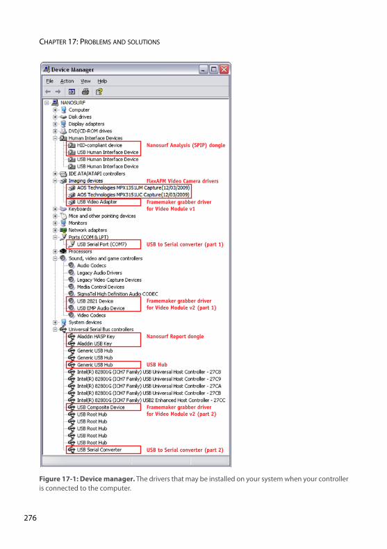
CHAPTER 17: PROBLEMS AND SOLUTIONS
27
Figure 17-1: Device manager. The drivers that may be installed on your system when your controlleris connected to the computer.
Nanosurf Analysis (SPIP) dongle
Framemaker grabber driverfor Video Module v1
USB to Serial converter (part 1)
Framemaker grabber driverfor Video Module v2 (part 1)
Nanosurf Report dongle
USB Hub
Framemaker grabber driverfor Video Module v2 (part 2)
USB to Serial converter (part 2)
FlexAFM Video Camera drivers
6
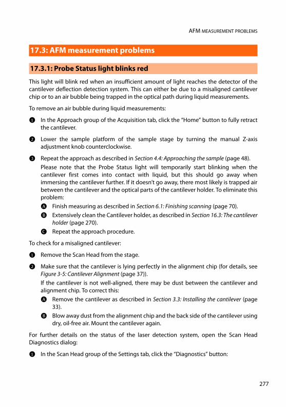
AFM MEASUREMENT PROBLEMS
This light will blink red when an insufficient amount of light reaches the detector of thecantilever deflection detection system. This can either be due to a misaligned cantileverchip or to an air bubble being trapped in the optical path during liquid measurements.
To remove an air bubble during liquid measurements:
1 In the Approach group of the Acquisition tab, click the “Home” button to fully retractthe cantilever.
2 Lower the sample platform of the sample stage by turning the manual Z-axisadjustment knob counterclockwise.
3 Repeat the approach as described in Section 4.4: Approaching the sample (page 48).Please note that the Probe Status light will temporarily start blinking when thecantilever first comes into contact with liquid, but this should go away whenimmersing the cantilever further. If it doesn’t go away, there most likely is trapped airbetween the cantilever and the optical parts of the cantilever holder. To eliminate thisproblem:A Finish measuring as described in Section 6.1: Finishing scanning (page 70).B Extensively clean the Cantilever holder, as described in Section 16.3: The cantilever
holder (page 270).C Repeat the approach procedure.
To check for a misaligned cantilever:
1 Remove the Scan Head from the stage.
2 Make sure that the cantilever is lying perfectly in the alignment chip (for details, seeFigure 3-5: Cantilever Alignment (page 37)).If the cantilever is not well-aligned, there may be dust between the cantilever andalignment chip. To correct this:A Remove the cantilever as described in Section 3.3: Installing the cantilever (page
33).B Blow away dust from the alignment chip and the back side of the cantilever using
dry, oil-free air. Mount the cantilever again.
For further details on the status of the laser detection system, open the Scan HeadDiagnostics dialog:
1 In the Scan Head group of the Settings tab, click the “Diagnostics” button:
17.3: AFM measurement problems
17.3.1: Probe Status light blinks red
277
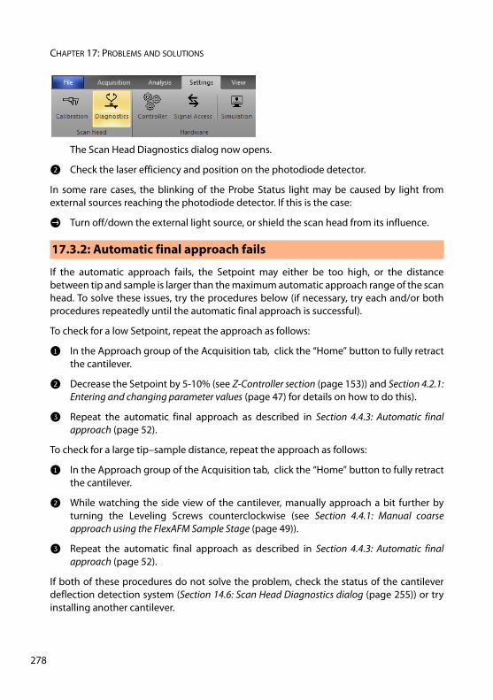
CHAPTER 17: PROBLEMS AND SOLUTIONS
27
The Scan Head Diagnostics dialog now opens.
2 Check the laser efficiency and position on the photodiode detector.
In some rare cases, the blinking of the Probe Status light may be caused by light fromexternal sources reaching the photodiode detector. If this is the case:
> Turn off/down the external light source, or shield the scan head from its influence.
If the automatic approach fails, the Setpoint may either be too high, or the distancebetween tip and sample is larger than the maximum automatic approach range of the scanhead. To solve these issues, try the procedures below (if necessary, try each and/or bothprocedures repeatedly until the automatic final approach is successful).
To check for a low Setpoint, repeat the approach as follows:
1 In the Approach group of the Acquisition tab, click the “Home” button to fully retractthe cantilever.
2 Decrease the Setpoint by 5-10% (see Z-Controller section (page 153)) and Section 4.2.1:Entering and changing parameter values (page 47) for details on how to do this).
3 Repeat the automatic final approach as described in Section 4.4.3: Automatic finalapproach (page 52).
To check for a large tip–sample distance, repeat the approach as follows:
1 In the Approach group of the Acquisition tab, click the “Home” button to fully retractthe cantilever.
2 While watching the side view of the cantilever, manually approach a bit further byturning the Leveling Screws counterclockwise (see Section 4.4.1: Manual coarseapproach using the FlexAFM Sample Stage (page 49)).
3 Repeat the automatic final approach as described in Section 4.4.3: Automatic finalapproach (page 52).
If both of these procedures do not solve the problem, check the status of the cantileverdeflection detection system (Section 14.6: Scan Head Diagnostics dialog (page 255)) or tryinstalling another cantilever.
17.3.2: Automatic final approach fails
8
NANOSURF SUPPORT
Tip picks up material
When a scan line suddenly starts reproducing badly, the tip may have picked up someparticles.
To get rid of these particles, follow the procedure below until the image quality improves:
1 Continue measuring for a while (1–2 images), as the tip may eventually lose theseparticles again.
2 In the Approach group of the Acquisition tab, click the “Withdraw” button to retractthe cantilever, and then perform a new approach.
3 Try to induce changes in the tip end: A While measuring, increase the force “Setpoint”, or decrease the amplitude
“Setpoint” in the Z-Controller section of the Imaging window. B Restore the Setpoint to its old value when the contrast improves, or if nothing
happens after scanning several lines.
4 Change the cantilever if no improvement occurs after following the steps above.
Setpoint drift
When part of the scan line in the Line graph is drawn red, the tip has moved to its maximumor minimum Z-position. This should also be visible in the range display on the right handside of the graph. The tip will move to its maximum Z-position when it has lost contact withthe sample. To correct this:
1 In the Static Force based modes, increase the force Setpoint, in the Dynamic Forcebased modes, reduce the amplitude Setpoint.
2 If this does not help, retract and re-approach the tip.
The fastest way to solve a problem is often to solve it yourself. If the previously suggestedactions did not help, or the problem is not described here, refer to the Nanosurf supportpages:
1 Open www.nanosurf.com.
2 Click on “Support”.
17.3.3: Image quality suddenly deteriorates
17.4: Nanosurf support
17.4.1: Self help
279
CHAPTER 17: PROBLEMS AND SOLUTIONS
28
3 Enter the login and password combination that you received upon registering.
4 Select the Easyscan 2 link.
5 If the problem is software related, try to upgrade to the latest version and/or read the“SPM Software Version History” to see if the problem was solved. For the solution toother problems, refer to the Frequently Asked Questions (FAQ).
If your instrument has not been registered yet, you will first have to register to receive apassword.
If the standard solutions are not sufficient, contact your local distributor for help. In orderto resolve the problem as fast as possible, please provide as much information as possible,such as:• A detailed description of what happened before the problem occurred. For example:
“When I click the ‘Approach’ button, then quickly click abort, the controller will not reactto anything I do anymore. This only happens when measuring in Dynamic Force Mode.”
• If an error message was displayed: The exact text of the message, or at least the start ofthe message.
• The serial number of your scan head and/or controller.• A description of the computer hardware and software on which the control software is
running: computer brand, type (laptop or desktop), operating system, software versionetc.
• Original Nanosurf image data (.nid) files that show the problem, rather than bitmapscreen shots, because these files contain all the settings that were used to make them.
• Parameter (.par) files with the instrument settings that were used when the problemoccurred.
• Script files, if the problem occurs during the operation of a script.
17.4.2: Assistance
IMPORANTSending “.vbs” scripts by e-mail often does not work, because these files are usuallyblocked as a security measure. To successfully e-mail a script, you may either:• Add the script text to the body of the e-mail.• Change the extension of the script file to “.txt” and attach it to the e-mail.• Compress the script file to a “.zip” archive and attach it to the e-mail.
0
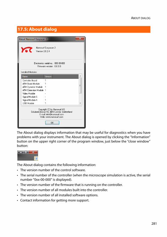
ABOUT DIALOG
The About dialog displays information that may be useful for diagnostics when you haveproblems with your instrument. The About dialog is opened by clicking the “Information”button on the upper right corner of the program window, just below the “close window”button:
The About dialog contains the following information: • The version number of the control software. • The serial number of the controller (when the microscope simulation is active, the serial
number “0xx-00-000” is displayed). • The version number of the firmware that is running on the controller.• The version number of all modules built into the controller.• The version number of all installed software options.• Contact information for getting more support.
17.5: About dialog
281

CHAPTER 17: PROBLEMS AND SOLUTIONS
28
2
CHAPTER 18:
AFM theory0
0
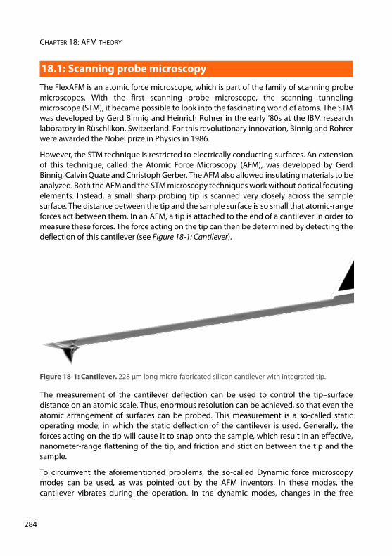
CHAPTER 18: AFM THEORY
28
The FlexAFM is an atomic force microscope, which is part of the family of scanning probemicroscopes. With the first scanning probe microscope, the scanning tunnelingmicroscope (STM), it became possible to look into the fascinating world of atoms. The STMwas developed by Gerd Binnig and Heinrich Rohrer in the early ’80s at the IBM researchlaboratory in Rüschlikon, Switzerland. For this revolutionary innovation, Binnig and Rohrerwere awarded the Nobel prize in Physics in 1986.
However, the STM technique is restricted to electrically conducting surfaces. An extensionof this technique, called the Atomic Force Microscopy (AFM), was developed by GerdBinnig, Calvin Quate and Christoph Gerber. The AFM also allowed insulating materials to beanalyzed. Both the AFM and the STM microscopy techniques work without optical focusingelements. Instead, a small sharp probing tip is scanned very closely across the samplesurface. The distance between the tip and the sample surface is so small that atomic-rangeforces act between them. In an AFM, a tip is attached to the end of a cantilever in order tomeasure these forces. The force acting on the tip can then be determined by detecting thedeflection of this cantilever (see Figure 18-1: Cantilever).
The measurement of the cantilever deflection can be used to control the tip–surfacedistance on an atomic scale. Thus, enormous resolution can be achieved, so that even theatomic arrangement of surfaces can be probed. This measurement is a so-called staticoperating mode, in which the static deflection of the cantilever is used. Generally, theforces acting on the tip will cause it to snap onto the sample, which result in an effective,nanometer-range flattening of the tip, and friction and stiction between the tip and thesample.
To circumvent the aforementioned problems, the so-called Dynamic force microscopymodes can be used, as was pointed out by the AFM inventors. In these modes, thecantilever vibrates during the operation. In the dynamic modes, changes in the free
18.1: Scanning probe microscopy
Figure 18-1: Cantilever. 228 μm long micro-fabricated silicon cantilever with integrated tip.
4
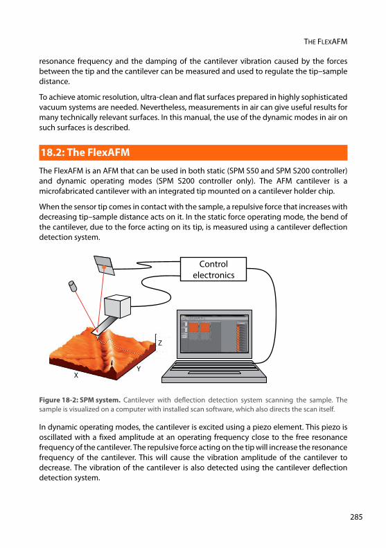
THE FLEXAFM
resonance frequency and the damping of the cantilever vibration caused by the forcesbetween the tip and the cantilever can be measured and used to regulate the tip–sampledistance.
To achieve atomic resolution, ultra-clean and flat surfaces prepared in highly sophisticatedvacuum systems are needed. Nevertheless, measurements in air can give useful results formany technically relevant surfaces. In this manual, the use of the dynamic modes in air onsuch surfaces is described.
The FlexAFM is an AFM that can be used in both static (SPM S50 and SPM S200 controller)and dynamic operating modes (SPM S200 controller only). The AFM cantilever is amicrofabricated cantilever with an integrated tip mounted on a cantilever holder chip.
When the sensor tip comes in contact with the sample, a repulsive force that increases withdecreasing tip–sample distance acts on it. In the static force operating mode, the bend ofthe cantilever, due to the force acting on its tip, is measured using a cantilever deflectiondetection system.
In dynamic operating modes, the cantilever is excited using a piezo element. This piezo isoscillated with a fixed amplitude at an operating frequency close to the free resonancefrequency of the cantilever. The repulsive force acting on the tip will increase the resonancefrequency of the cantilever. This will cause the vibration amplitude of the cantilever todecrease. The vibration of the cantilever is also detected using the cantilever deflectiondetection system.
18.2: The FlexAFM
Figure 18-2: SPM system. Cantilever with deflection detection system scanning the sample. Thesample is visualized on a computer with installed scan software, which also directs the scan itself.
Controlelectronics
XY
Z
285
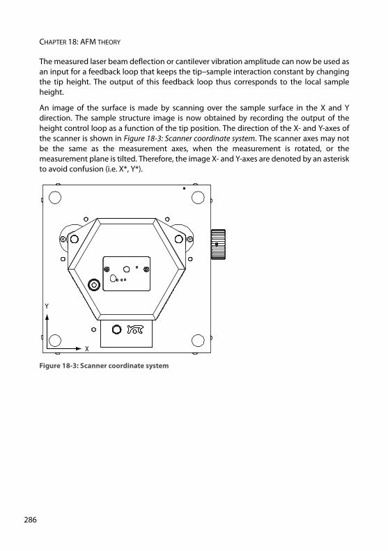
CHAPTER 18: AFM THEORY
28
The measured laser beam deflection or cantilever vibration amplitude can now be used asan input for a feedback loop that keeps the tip–sample interaction constant by changingthe tip height. The output of this feedback loop thus corresponds to the local sampleheight.
An image of the surface is made by scanning over the sample surface in the X and Ydirection. The sample structure image is now obtained by recording the output of theheight control loop as a function of the tip position. The direction of the X- and Y-axes ofthe scanner is shown in Figure 18-3: Scanner coordinate system. The scanner axes may notbe the same as the measurement axes, when the measurement is rotated, or themeasurement plane is tilted. Therefore, the image X- and Y-axes are denoted by an asteriskto avoid confusion (i.e. X*, Y*).
Figure 18-3: Scanner coordinate system
X
Y
6

CHAPTER 19:
Technical data0
0
0
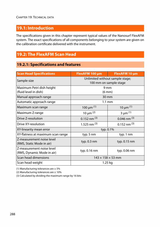
CHAPTER 19: TECHNICAL DATA
28
The specifications given in this chapter represent typical values of the Nanosurf FlexAFMsystem. The exact specifications of all components belonging to your system are given onthe calibration certificate delivered with the instrument.
19.1: Introduction
19.2: The FlexAFM Scan Head
19.2.1: Specifications and features
Scan Head Specifications FlexAFM 100 μm FlexAFM 10 μm
Sample sizeUnlimited without sample stage;
100 mm on sample stageMaximum Petri dish height(fluid level in dish)
9 mm(6 mm)
Manual approach range 30 mmAutomatic approach range 1.1 mm
Maximum scan range 100 μm (1) 10 μm (1)
Maximum Z-range 10 μm (2) 3 μm (1)
Drive Z-resolution 0.152 nm (3) 0.046 nm (3)
Drive XY-resolution 1.525 nm (3) 0.152 nm (3)
XY-linearity mean error typ. 0.1%XY-flatness at maximum scan range typ. 5 nm typ. 1 nmZ-measurement noise level (RMS, Static Mode in air)
typ. 0.3 nm typ. 0.15 nm
Z-measurement noise level (RMS, Dynamic Mode in air)
typ. 0.16 nm typ. 0.06 nm
Scan head dimensions 143 × 158 × 53 mmScan head weight 1.25 kg
(1) Manufacturing tolerances are ± 5%(2) Manufacturing tolerances are ± 10%(3) Calculated by dividing the maximum range by 16 bits
8
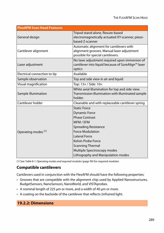
THE FLEXAFM SCAN HEAD
Compatible cantilevers
Cantilevers used in conjunction with the FlexAFM should have the following properties: • Grooves that are compatible with the alignment chip used by Applied Nanostructures,
BudgetSensors, NanoSensors, NanoWorld, and VISTAprobes.• A nominal length of 225 μm or more, and a width of 40 μm or more.• A coating on the backside of the cantilever that reflects (infra)red light.
FlexAFM Scan Head Features
General designTripod stand-alone, flexure-based electromagnetically actuated XY-scanner, piezo-based Z-scanner
Cantilever alignmentAutomatic alignment for cantilevers with alignment grooves. Manual laser adjustment possible for special cantilevers.
Laser adjustmentNo laser adjustment required upon immersion of cantilever into liquid because of SureAlign™ laser optics
Electrical connection to tip AvailableSample observation Top and side view in air and liquidVisual magnification Top: 13× / Side: 10×
Sample illuminationWhite axial illumination for top and side view. Transmission illumination with illuminated sample holder.
Cantilever holder Cleanable and with replaceable cantilever spring
Operating modes (1)
Static ForceDynamic ForcePhase ContrastMFM / EFMSpreading ResistanceForce ModulationLateral ForceKelvin Probe ForceScanning ThermalMultiple Spectroscopy modesLithography and Manipulation modes
(1) See Table 8-1: Operating modes and required modules (page 90) for required modules
19.2.2: Dimensions
289
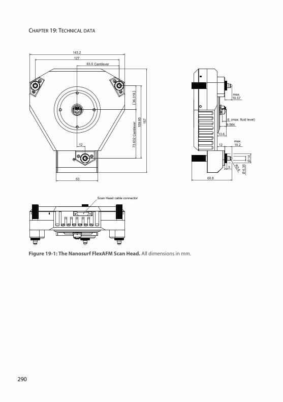
CHAPTER 19: TECHNICAL DATA
29
Figure 19-1: The Nanosurf FlexAFM Scan Head. All dimensions in mm.
6 (max. fluid level)
10.57max.
10.2max.
60.8
12
3
13.6
Ø14
Ø6.
35
R2.4
9.564
127
143.2
12
63
73.6
32 C
antil
ever 15
710
9.95
36.3
18
63.5 Cantilever
Scan Head cable connector
0
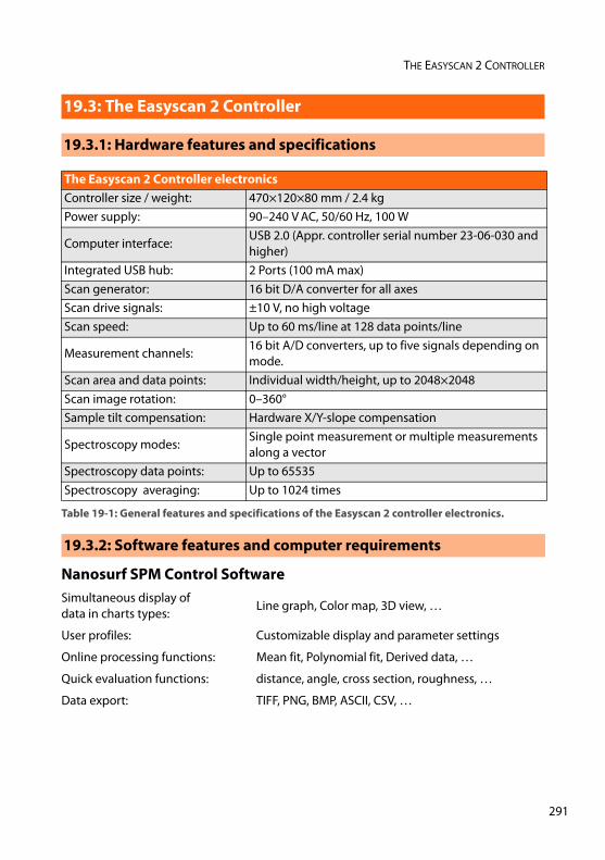
THE EASYSCAN 2 CONTROLLER
Nanosurf SPM Control Software
19.3: The Easyscan 2 Controller
19.3.1: Hardware features and specifications
The Easyscan 2 Controller electronicsController size / weight: 470×120×80 mm / 2.4 kgPower supply: 90–240 V AC, 50/60 Hz, 100 W
Computer interface:USB 2.0 (Appr. controller serial number 23-06-030 and higher)
Integrated USB hub: 2 Ports (100 mA max)Scan generator: 16 bit D/A converter for all axesScan drive signals: ±10 V, no high voltageScan speed: Up to 60 ms/line at 128 data points/line
Measurement channels:16 bit A/D converters, up to five signals depending on mode.
Scan area and data points: Individual width/height, up to 2048×2048 Scan image rotation: 0–360°Sample tilt compensation: Hardware X/Y-slope compensation
Spectroscopy modes:Single point measurement or multiple measurements along a vector
Spectroscopy data points: Up to 65535Spectroscopy averaging: Up to 1024 times
Table 19-1: General features and specifications of the Easyscan 2 controller electronics.
19.3.2: Software features and computer requirements
Simultaneous display ofdata in charts types:
Line graph, Color map, 3D view, …
User profiles: Customizable display and parameter settings
Online processing functions: Mean fit, Polynomial fit, Derived data, …
Quick evaluation functions: distance, angle, cross section, roughness, …
Data export: TIFF, PNG, BMP, ASCII, CSV, …
291
CHAPTER 19: TECHNICAL DATA
29
Nanosurf Scripting Interface
The Scripting Interface has to be purchased separately for Easyscan 2 systems.
Lithography can also be performed via the scripting interface, but is more easily performedvia the Lithography Window of the control software, or (when more advanced options arerequired) by purchasing the Lithography Option.
Computer requirements
For a detailed description of computer hardware requirements and supported operatingsystems, see Nanosurf technical note “TN00477 — Computer requirements for NanosurfProducts”. The technical note can be downloaded from the Support section of the Nanosurfwebsite by all registered users.
Applications:Automating measurement tasks, custom evaluation functions, using third party measurement equipment, …
Included control software:Windows Scripting Host: Visual Basic Script, Java Script, …
Remote control by:COM compatible languages: LabView, MathLab, Visual Basic, Delphi, C++, …
2
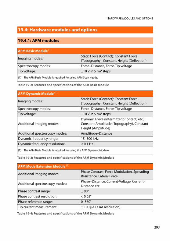
HARDWARE MODULES AND OPTIONS
19.4: Hardware modules and options
19.4.1: AFM modules
AFM Basic Module (1)
Imaging modes:Static Force (Contact): Constant Force (Topography), Constant Height (Deflection)
Spectroscopy modes: Force–Distance, Force-Tip voltageTip voltage: ±10 V in 5 mV steps
(1) The AFM Basic Module is required for using AFM Scan Heads.
Table 19-2: Features and specifications of the AFM Basic Module
AFM Dynamic Module (1)
Imaging modes:Static Force (Contact): Constant Force (Topography), Constant Height (Deflection)
Spectroscopy modes: Force–Distance, Force-Tip voltageTip voltage: ±10 V in 5 mV steps
Additional imaging modes:Dynamic Force (Intermittent Contact, etc.): Constant Amplitude (Topography), Constant Height (Amplitude)
Additional spectroscopy modes: Amplitude–DistanceDynamic frequency range: 15–500 kHzDynamic frequency resolution: < 0.1 Hz
(1) The AFM Basic Module is required for using the AFM Dynamic Module.
Table 19-3: Features and specifications of the AFM Dynamic Module
AFM Mode Extension Module (1)
Additional imaging modes:Phase Contrast, Force Modulation, Spreading Resistance, Lateral Force
Additional spectroscopy modes:Phase–Distance, Current-Voltage, Current–Distance etc.
Phase contrast range: ± 90°Phase contrast resolution: < 0.05°Phase reference range: 0–360°Tip current measurement: ± 100 μA (3 nA resolution)
Table 19-4: Features and specifications of the AFM Dynamic Module
293
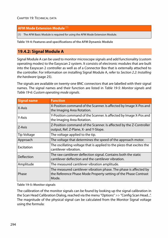
CHAPTER 19: TECHNICAL DATA
29
Signal Module A can be used to monitor microscope signals and add functionality (customoperating modes) to the Easyscan 2 system. It consists of electronic modules that are builtinto the Easyscan 2 controller as well as of a Connector Box that is externally attached tothe controller. For information on installing Signal Module A, refer to Section 2.2: Installingthe hardware (page 25).
The signals are available on twenty-one BNC connectors that are labelled with their signalnames. The signal names and their function are listed in Table 19-5: Monitor signals andTable 19-6: Custom operating mode signals.
The calibration of the monitor signals can be found by looking up the signal calibration inthe Scan Head Calibration Dialog, reached via the menu “Options” >> “Config Scan Head...”.The magnitude of the physical signal can be calculated from the Monitor Signal voltageusing the formula:
(1) The AFM Basic Module is required for using the AFM Mode Extension Module.
19.4.2: Signal Module A
Signal name Function
X-AxisX-Position command of the Scanner. Is affected by Image X-Pos and the Imaging Area Rotation.
Y-AxisY-Position command of the Scanner. Is affected by Image X-Pos and the Imaging Area Rotation.
Z-AxisZ-Position command of the Scanner. Is affected by the Z-Controller output, Ref. Z-Plane, X- and Y-Slope.
Tip Voltage The voltage applied to the tip.Approach The voltage that determines the speed of the approach motor.
ExcitationThe oscillating voltage that is applied to the piezo that excites the cantilever vibration.
DeflectionThe raw cantilever deflection signal. Contains both the static cantilever deflection and the cantilever vibration.
Amplitude The measured cantilever vibration amplitude.
PhaseThe measured cantilever vibration phase. The phase is affected by the Reference Phase Mode Property setting of the Phase Contrast Mode.
Table 19-5: Monitor signals
AFM Mode Extension Module (1)
Table 19-4: Features and specifications of the AFM Dynamic Module
4
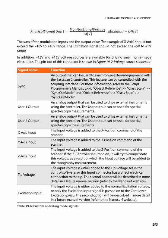
HARDWARE MODULES AND OPTIONS
The sum of the modulation inputs and the output value (for example of X-Axis) should notexceed the –10V to +10V range. The Excitation signal should not exceed the –5V to +5Vrange.
In addition, –15V and +15V voltage sources are available for driving small home-madeelectronics. The pin-out of this connector is shown in Figure 19-2: Voltage source connector.
Signal name Function
Sync
An output that can be used to synchronize external equipment with the Easyscan 2 controller. This feature can be controlled with the scripting interface. For more information, refer to the Script Programmers Manual, topic “Object Reference” >> “Class Scan” >> “SyncOutMode” and “Object Reference” >> “Class Spec” >> “SyncOutMode”
User 1 OutputAn analog output that can be used to drive external instruments using the controller. The User output can be used for special spectroscopy measurements.
User 2 OutputAn analog output that can be used to drive external instruments using the controller. The User output can be used for special spectroscopy measurements.
X-Axis InputThe Input voltage is added to the X-Position command of the scanner.
Y-Axis InputThe Input voltage is added to the Y-Position command of the scanner.
Z-Axis Input
The Input voltage is added to the Z-Position command of the scanner. If the Z-Controller is turned on, it will try to compensate this voltage, as a result of which the Input voltage will be added to the topography measurement.
Tip Voltage
The input voltage is either added to the Tip-voltage set in the control software, or this Input connector has a direct electrical connection to the tip. The second option will be described in more detail in a future manual version (refer to the Nanosurf website).
Excitation Input
The input voltage is either added to the normal Excitation voltage, or only the Excitation Input signal is passed on to the Cantilever Excitation piezo. The second option will be described in more detail in a future manual version (refer to the Nanosurf website).
Table 19-6: Custom operating mode signals.
PhysicalSignal Unit[ ] MonitorSignalVoltage10 V[ ]
----------------------------------------------------------- Maximum Offset+⋅=
295
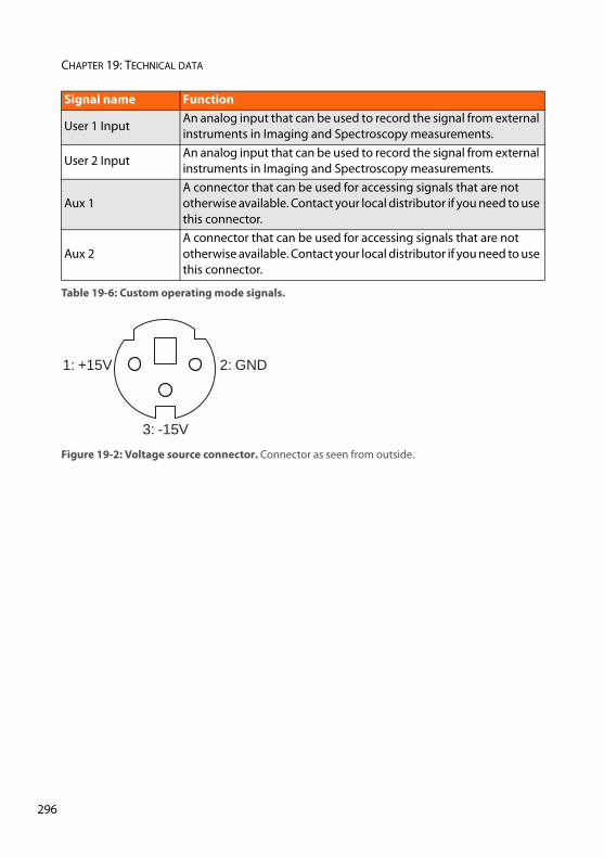
CHAPTER 19: TECHNICAL DATA
29
User 1 InputAn analog input that can be used to record the signal from external instruments in Imaging and Spectroscopy measurements.
User 2 InputAn analog input that can be used to record the signal from external instruments in Imaging and Spectroscopy measurements.
Aux 1A connector that can be used for accessing signals that are not otherwise available. Contact your local distributor if you need to use this connector.
Aux 2A connector that can be used for accessing signals that are not otherwise available. Contact your local distributor if you need to use this connector.
Figure 19-2: Voltage source connector. Connector as seen from outside.
Signal name Function
Table 19-6: Custom operating mode signals.
2: GND
3: -15V
1: +15V
6
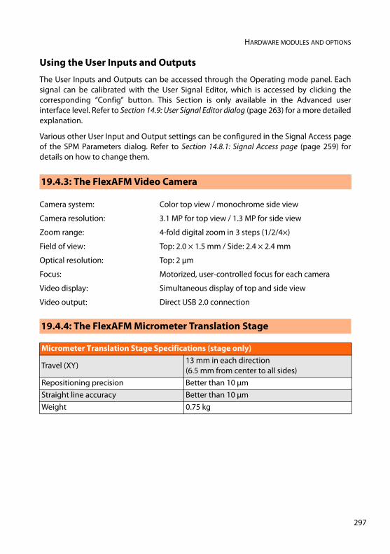
HARDWARE MODULES AND OPTIONS
Using the User Inputs and Outputs
The User Inputs and Outputs can be accessed through the Operating mode panel. Eachsignal can be calibrated with the User Signal Editor, which is accessed by clicking thecorresponding “Config” button. This Section is only available in the Advanced userinterface level. Refer to Section 14.9: User Signal Editor dialog (page 263) for a more detailedexplanation.
Various other User Input and Output settings can be configured in the Signal Access pageof the SPM Parameters dialog. Refer to Section 14.8.1: Signal Access page (page 259) fordetails on how to change them.
19.4.3: The FlexAFM Video Camera
Camera system: Color top view / monochrome side view
Camera resolution: 3.1 MP for top view / 1.3 MP for side view
Zoom range: 4-fold digital zoom in 3 steps (1/2/4×)
Field of view: Top: 2.0 × 1.5 mm / Side: 2.4 × 2.4 mm
Optical resolution: Top: 2 μm
Focus: Motorized, user-controlled focus for each camera
Video display: Simultaneous display of top and side view
Video output: Direct USB 2.0 connection
19.4.4: The FlexAFM Micrometer Translation Stage
Micrometer Translation Stage Specifications (stage only)
Travel (XY)13 mm in each direction(6.5 mm from center to all sides)
Repositioning precision Better than 10 μmStraight line accuracy Better than 10 μmWeight 0.75 kg
297

CHAPTER 19: TECHNICAL DATA
29
8


![UEL Library Search [Catalogue]](https://img.pdfslide.us/doc/110x75/56812d9d550346895d92bb8a/uel-library-search-catalogue.jpg)