Embed Size (px)
Citation preview
Nanoscale structure and mechanical properties of a Soft Material
by
Hossein Salahshoor Pirsoltan
A Thesis
of the
WORCESTER POLYTECHNIC INSTITUTE
in partial fulfillment of the requirements for the
Degree of Master of Science
In
Civil Engineering
May 2013
APPROVED:
Dr. Nima Rahbar, Thesis Advisor
Dr. Nathaniel A. Deskins, Committee Member
Dr. Qi Wen, Committee Member
Dr. Mazdak P. Tootkaboni, Committee Member
i
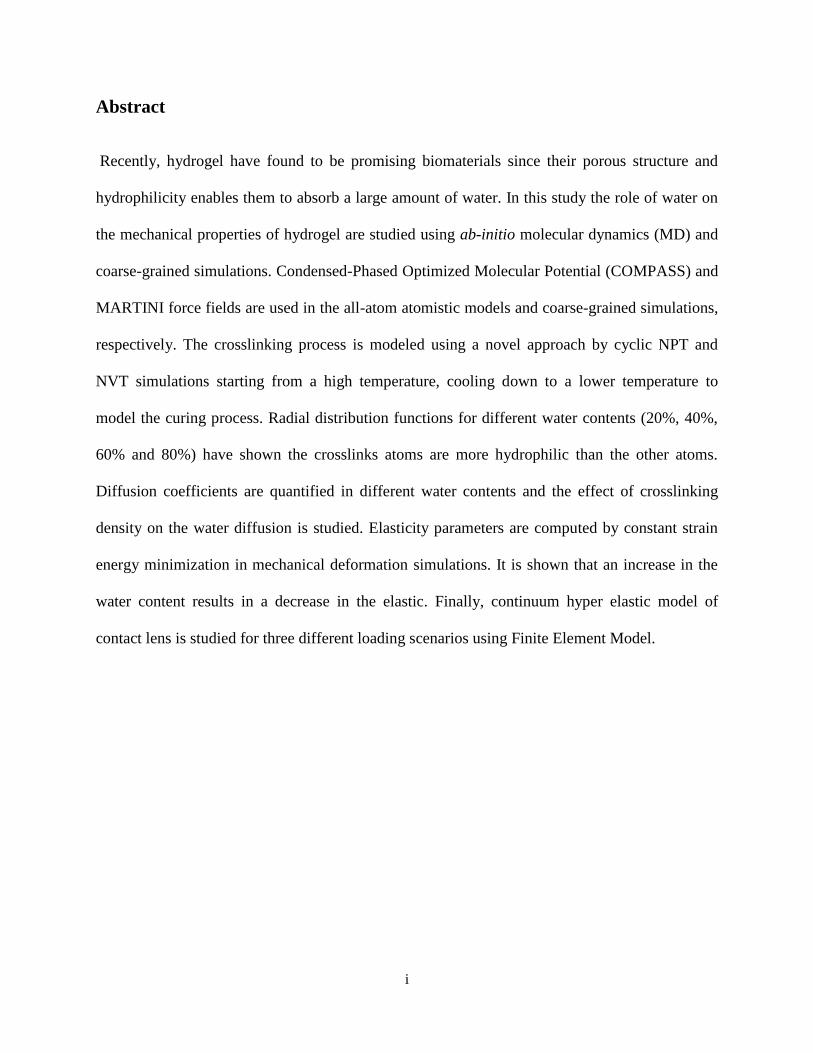
Abstract
Recently, hydrogel have found to be promising biomaterials since their porous structure and
hydrophilicity enables them to absorb a large amount of water. In this study the role of water on
the mechanical properties of hydrogel are studied using ab-initio molecular dynamics (MD) and
coarse-grained simulations. Condensed-Phased Optimized Molecular Potential (COMPASS) and
MARTINI force fields are used in the all-atom atomistic models and coarse-grained simulations,
respectively. The crosslinking process is modeled using a novel approach by cyclic NPT and
NVT simulations starting from a high temperature, cooling down to a lower temperature to
model the curing process. Radial distribution functions for different water contents (20%, 40%,
60% and 80%) have shown the crosslinks atoms are more hydrophilic than the other atoms.
Diffusion coefficients are quantified in different water contents and the effect of crosslinking
density on the water diffusion is studied. Elasticity parameters are computed by constant strain
energy minimization in mechanical deformation simulations. It is shown that an increase in the
water content results in a decrease in the elastic. Finally, continuum hyper elastic model of
contact lens is studied for three different loading scenarios using Finite Element Model.
ii
Acknowledgements
I would like to thank my thesis advisor Dr. Nima Rahbar for all his help, support, and
guidance throughout the last two years of conducting research. I also would like to thank Dr.
Mazdak Tootkaboni, as my previous major advisor in University of Massachusetts Dartmouth,
for all his support and guidance. Also thanks to the committee members, Dr. Deskins and Dr.
Wen for their guidance.
I would also like to thank the rest of the faculty and my friends especially my lab mates,
for allowing me to have a great experience.
Lastly, I would like to thank my parents and siblings, for their continued support over the
last 24 years. I wouldn’t have been able to accomplish all that I have without their support and
advice.
iii
Table of Contents
Abstract ………………………………………………………………………………………… i
Acknowledgments ……………………………………………………………………………... ii
Table of Contents ……………………………………………………………………………… iii
List of Tables …………………………………………………………………………………... vi
List of Figures ………………………………………………………………………………….. vii
1. Introduction …………………………………………………………………………………. 1
1.1. Hydrogel …………………………………………………………………………... 1
1.2. Atomistic Modeling ……………………………………………………………….. 2
1.3 Objectives ………………………………………………………………………….. 6
2. Computational Backgrounds ………………………………………………………………... 7
2.1. Molecular Dynamics Simulations ………………………………………………… 7
2.1.1. Verlet Algorithm ………………………………………………………... 7
2.1.2. Ensembles ………………………………………………………………. 9
2.1.3. Energy Minimization …………………………………………………….9
2.1.4. Force Fields ……………………………………………………………...10
3. Atomistic Modeling of Crosslinked Polymers ……………………………………………....16
iv
3.1. Crosslinking Protocol ………………………………………………………………17
3.2. Results ………………………………………………………………………………19
4. All-Atom Molecular Dynamics Simulation…………………………………………………...23
4.1. Introduction …………………………………………………………………………23
4.2. Simulation Details …………………………………………………………………..24
4.2.1. Model Construction ………………………………………………………24
4.2.2. Crosslinking Process ……………………………………………………...25
4.2.3. Force Field and Simulation Parameters …………………………………..25
4.3. Results and Discussion ……………………………………………………………..28
4.3.1. Crosslinking Process ……………………………………………………...28
4.3.2. Equilibrated Structure and the Role of Water …………………………….30
4.3.3. Elastic Properties of Hydrogels …………………………………………..37
4.4. Conclusion ………………………………………………………………………….40
5. Coarse-Grained Model of Hydrogel ………………………………………………………….41
5.1. Introduction …………………………………………………………………………41
5.2. MARTINI Model ………………………………………………………………….. 41
5.2.1. Interaction Sites …………………………………………………………. 41
v
5.2.2. Bonded and Nonbonded Interactions …………………………………..42
5.3. Coarse-Grained Model for the Hydrogel ………………………………………….43
5.4. Results and Discussion …………………………………………………………….45
6. Hydrogels in Continuum Scale ………………………………………………………………50
6.1. Introduction ………………………………………………………………………..50
6.2 Mechanical Scenarios ……………………………………………………………….50
6.2.1. Case I: Point Load ………………………………………………………..50
6.2.2. Case II: Contact by a Rigid Plate …………………………………………54
6.2.3. Case III: Uniform Side Pressure ………………………………………….58
7. Summary…….…………………...…………………………………..………………………..62
8. Recommendations and Future Work …………………………………………………………63
9. References ……………………………………………………………………………………64

vi
List of Tables
Table 5-1: Cell dimensions, before and after the initial 10 ns minimization.
vii
List of Figures
Figure 1.The hierarchical multi-scale paradigm in molecular simulation……………………....3
Figure 2. Numerical Approach for MD Simulation…………………………………………….10
Figure 3. Bond Angle Bend…………………………………………………………………….12
Figure 4. Torsion Angle…………………………………………………………………………13
Figure 5. Scheme of Inversion…………………………………………………………………..13
Figure 6. The chemical structure of: (a) Diglycidyl Ether of Bisphenol-A (DGEBA); (b)
Aminoethyl Piperazine (AEP)…………………………………………………………………...17
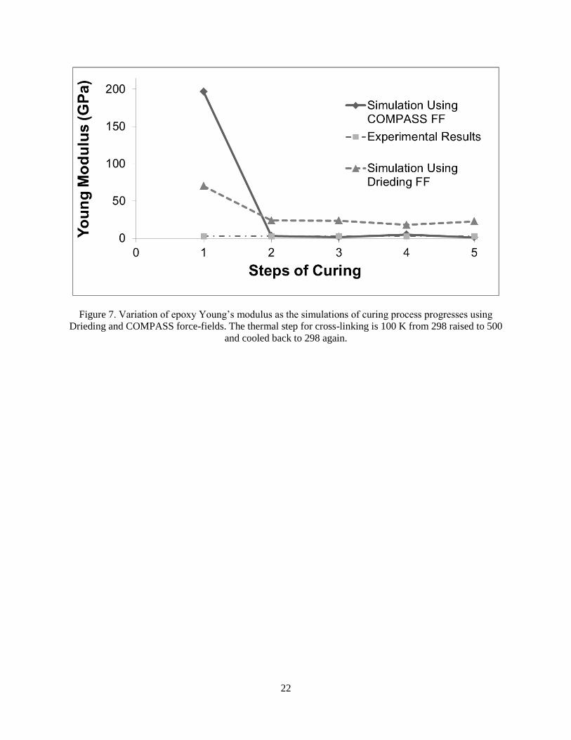
Figure 7. Variation of epoxy Young’s modulus as the simulations of curing process progresses
using Drieding and COMPASS force-fields. The thermal step for cross-linking is 100 K from
298 raised to 500 and cooled back to 298 again…………………………………………………22
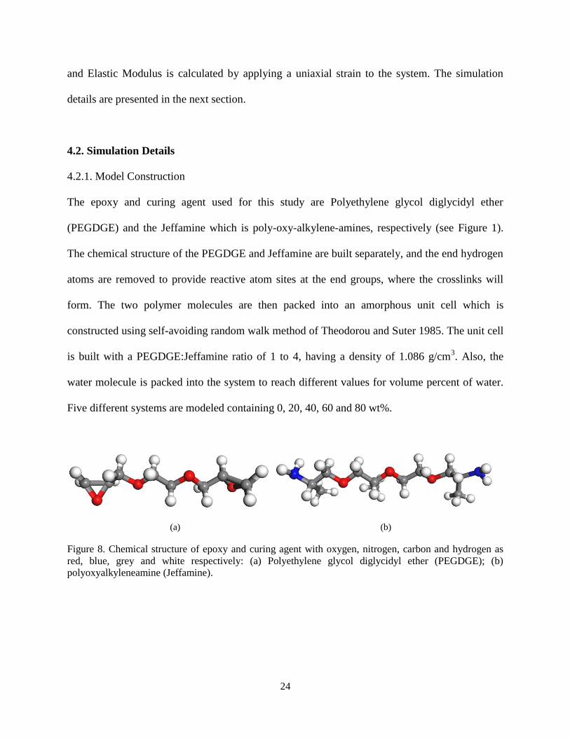
Figure 8. Chemical structure of epoxy and curing agent with oxygen, nitrogen, carbon and
hydrogen as red, blue, grey and white respectively: (a) Polyethylene glycol diglycidyl ether
(PEGDGE); (b) polyoxyalkyleneamine (Jeffamine)…………………………………………….24
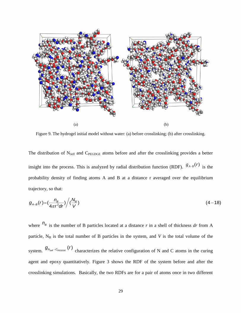
Figure 9. The hydrogel initial model without water: (a) before crosslinking; (b) after
crosslinking………………………………………………………………………………………29
Figure 10. Radial Distribution Function of NJeff – CPEGDGE pair for the initial model: (a)
before crosslinking; (b) after crosslinking……………………………………………………….30
viii
Figure 11. Equilibrated hydrogel structures: (a) 20 wt% before crosslinking ; (b) 20 wt% after
crosslinking; (c) 40 wt% before crosslinking ; (d) 40 wt% after crosslinking; (e) 60 wt% before
crosslinking ; (f) 60 wt% after crosslinking; (g) 80 wt% before crosslinking; (h) 80 wt% after
crosslinking………………………………………………………………………………………32
Figure 12. Radial Distribution Function for Oxygen-O(Water, Nitrogen-O(Water) and Carbon-
O(Water) pairs for different water contents: (a) 20 wt%; (b) 40 wt%; (c) 60 wt%; (d) 80 wt%..35
Figure 13. Diffusion coefficients for water molecules in different water contents, both before and
after crosslinking…………………………………………………………………………………37
Figure 14. Change in elastic modulus vs water content…………………………………………39
Figure 15. Coarse-Grain model for: (a) Jefffamine. (b) PEGDGE. The Nitrogen, Oxygen, Carbon
and Hydrogen atoms are shown in blue, red, grey and white, respectively……………………..44
Figure 16. CG model for the: (a) Jeffamine. (b)PEGDGE………………………………………45
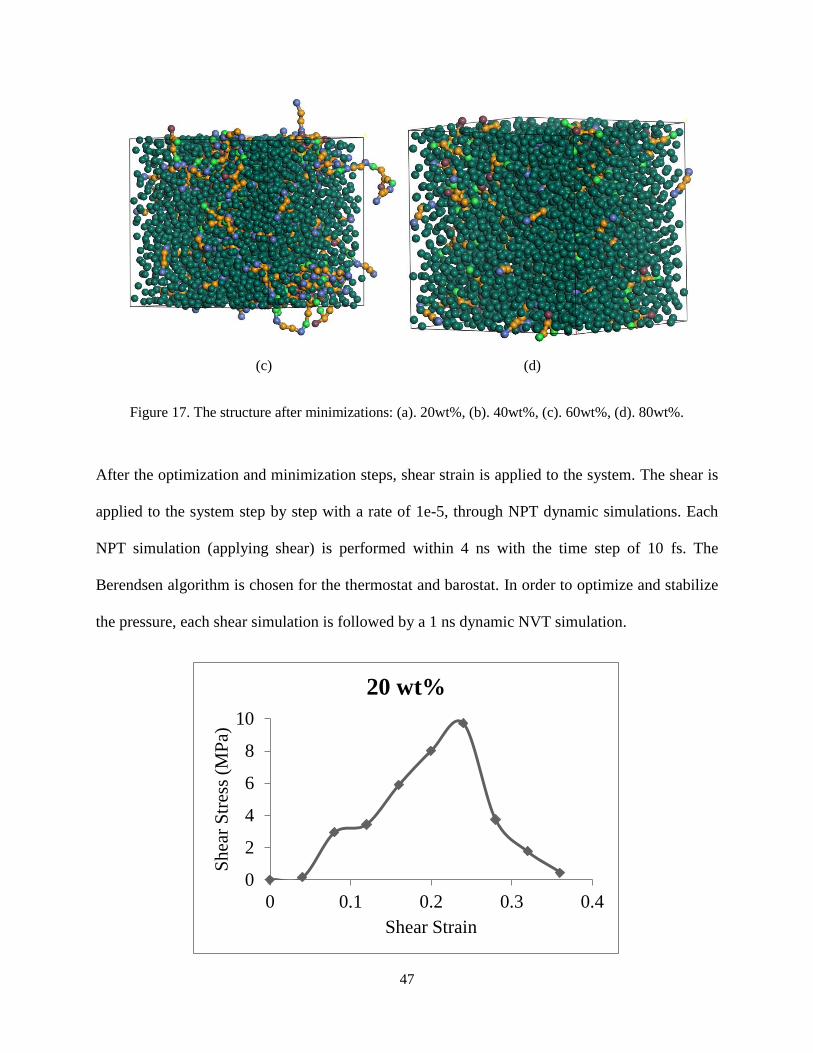
Figure 17. The structure after minimizations: (a). 20wt%, (b). 40wt%, (c). 60wt%, (d). 80wt%.47
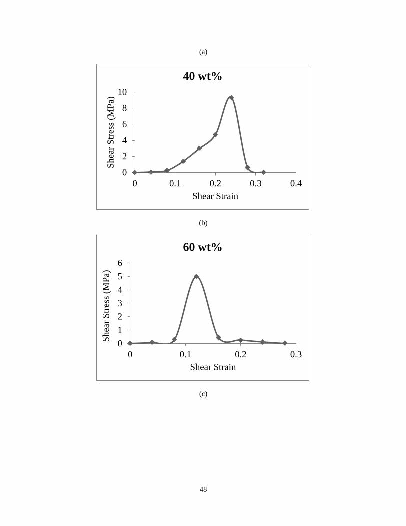
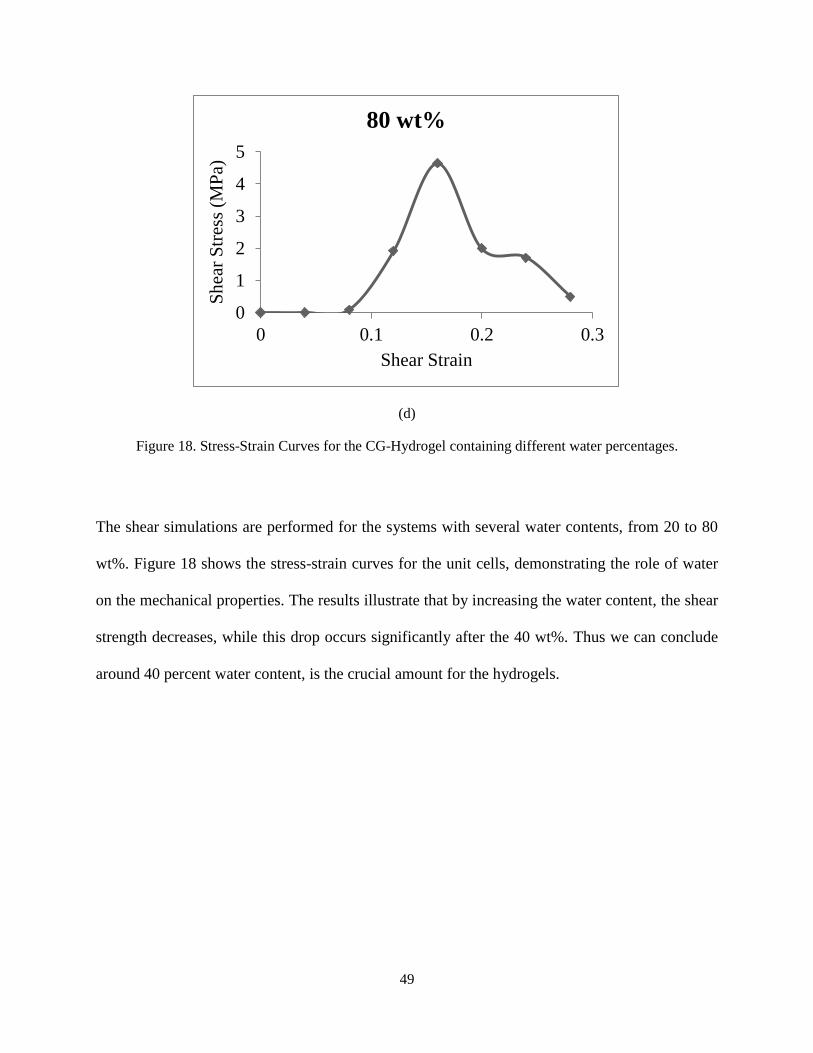
Figure 18. Stress-Strain Curves for the CG-Hydrogel containing different water percentages…49
Figure 19. Mesh assigned model and the load direction………………………………………...51
Figure 20. Hydrogel Deformation Due to The Point Load………………………………………53
Figure 21. Load-Displacement for the Hydrogel Due to The Point Load……………………….54
Figure 22. Initial Contact Model…………………………………………………………………55
Figure 23. Stress distribution due to the contact between hydrogel and rigid plate……………..57
ix
Figure 1. Force.vs.Displacement for the contact scenario……………………………………………….58
Figure 25. Uniform displacement model………………………………………………………………….59
Figure 26. Stress contour for the deformed hydrogel……………………………………………………..60
Figure 27. Force s Displacement for the hydrogel in the uniform displacement scenario………………..61
1
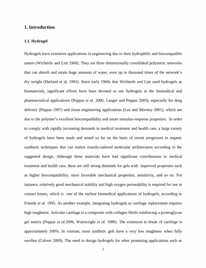
1. Introduction
1.1. Hydrogel
Hydrogels have extensive applications in engineering due to their hydrophilic and biocompatible
nature (Wichterle and Lim 1960). They are three dimensionally crosslinked polymeric networks
that can absorb and retain huge amounts of water, even up to thousand times of the network’s
dry weight (Harland et al, 1992). Since early 1960s that Wichterle and Lim used hydrogels as
biomaterials, significant efforts have been devoted to use hydrogels in the biomedical and
pharmaceutical applications (Peppas et al. 2000, Langer and Peppas 2003), especially for drug
delivery (Peppas 1997) and tissue engineering applications (Lee and Mooney 2001), which are
due to the polymer’s excellent biocompatibility and smart stimulus-response properties. In order
to comply with rapidly increasing demands in medical treatment and health care, a large variety
of hydrogels have been made and tested so far on the basis of recent progresses in organic
synthesis techniques that can realize exactly-tailored molecular architectures according to the
suggested design. Although these materials have had significant contributions to medical
treatment and health care, there are still strong demands for gels with improved properties such
as higher biocompatibility, more favorable mechanical properties, sensitivity, and so on. For
instance, relatively good mechanical stability and high oxygen permeability is required for use in
contact lenses, which is one of the earliest biomedical applications of hydrogels, according to
Friends et al. 1995. As another example, integrating hydrogels as cartilage replacement requires
high toughness. Articular cartilage is a composite with collagen fibrils reinforcing a proteoglycan
gel matrix (Peppas et al.2006, Wainwright et al. 1986). The extension to break of cartilage is
approximately 100%. In contrast, most synthetic gels have a very low toughness when fully
swollen (Calvert 2009). The need to design hydrogels for other promising applications such as
2
wound-healing bioadhesives, artificial kidney membranes, artificial skin, maxillofacial, sexual
organ reconstruction materials, and drug delivery vehicles is getting critical. There are various
approaches to improve properties of hydrogels: to redesign given synthetic materials, to
hybridize synthetic materials with biomaterials, and to modify given biomaterials. In order to
accomplish any of these, molecular mechanisms leading to physical properties of each class of
biomaterials need to be understood. Thus, we will focus on the understanding of the molecular
mechanisms at an atomic/molecular level to provide valuable information to design new
materials using computational approaches to obtain various desirable properties.
1.2. Atomistic Modeling
Computational science is one of the most promising and rapidly expanding branches of science.
Computers provide the opportunity to model different materials and study their chemical and
physical properties. Prior to the advent of computational approaches, various properties could
only be predicted using theoretical approaches that provided a crude description of materials.
Computer simulations, however, have provided useful information for problems in various fields
such as biology, chemistry, and physics, as well as economics and psychology after it played an
essential role in developing nuclear weapons and code breaking in the early 1950s (Frenkel and
Smith 2001), demonstrating its various capabilities. High performance computers have since
accelerated the growth of computational methods in almost every field of science and
technology.
Among various computer simulation methods, molecular and ab-initio simulation
methods have provided direct routes from the microscopic structural details of materials to the
3
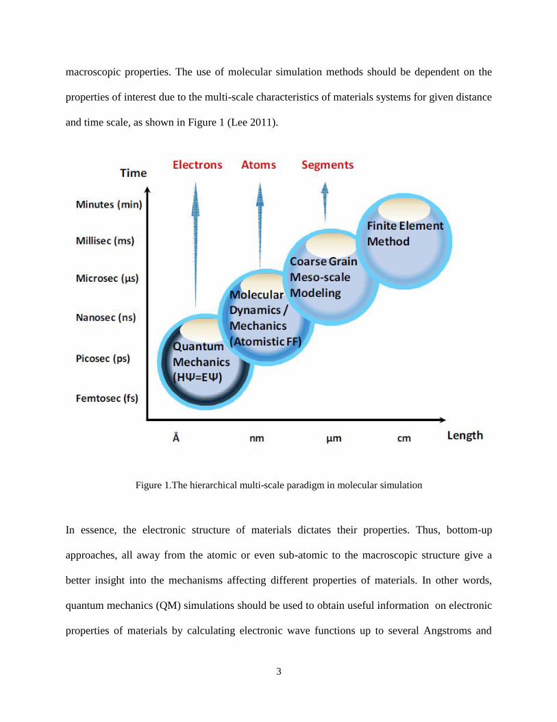
macroscopic properties. The use of molecular simulation methods should be dependent on the
properties of interest due to the multi-scale characteristics of materials systems for given distance
and time scale, as shown in Figure 1 (Lee 2011).
Figure 1.The hierarchical multi-scale paradigm in molecular simulation
In essence, the electronic structure of materials dictates their properties. Thus, bottom-up
approaches, all away from the atomic or even sub-atomic to the macroscopic structure give a
better insight into the mechanisms affecting different properties of materials. In other words,
quantum mechanics (QM) simulations should be used to obtain useful information on electronic
properties of materials by calculating electronic wave functions up to several Angstroms and
4
picoseconds. Since QM methods determine state of all electrons, QM results in accurate
geometries and energies of the system. Since, QM simulations are computationally expensive
and nearly impractical given today’s technology for systems containing over several hundreds
and thousands of atoms, a different approach is considered.
Quantum mechanics can be approximated with molecular mechanics (MM) and molecular
dynamics (MD) by averaging over the electron wave functions. This method allows us to
investigate the structure and energetic of larger systems with up to hundred nanometers in
dimension or even micron scales. In MM or MD, the atoms are considered as soft spheres
bonded to each other with springs. Energies and forces derived from this approximation can be
used in classical physics formulas to obtain dynamic trajectories, conformations or optimized
geometries. MD simulations allow for the study of comparatively large systems and have
emerged as an effective tool for the characterization of the mechanical and thermal behavior of
nanostructures.
Further up in the hierarchy, lie simulation methods requiring even more crude approximations to
maintain computational feasibility for systems operating on longer time and distance. Since
polymeric systems are complex, it is still not feasible to completely describe them using MD
technique. Chapter two discusses MD approach in more detail.
MD simulations have been extensively employed to characterize the molecular structure of
biomaterials. It should be noted however, that there have been only a limited number of MD
simulation studies on hydrogel systems.
Tamai and Tanaka carried out MD simulations for hydrogel models of poly(vinyl alcohol),
poly(vinyl methyl ether), and poly(N-isopropylacrylamide) hydrogels to study polymer-water
5
interaction in hydrogels by analyzing the hydrogen bond structure and dynamics. The range for
degree of polymerization (DP) of the polymer chain is 11-161 and the range for number of water
molecules is 5 to 215. They have also performed MD simulations of poly(vinyl alcohol) with 81
or 161 DP and pure water over a wide temperature range of 150-400 K to study effects of
polymer chains on structure and dynamics of supercooled water in hydrogels. They used 150 to
216 water molecules and a simulation time range of 1 to 40 ns.
Oldiges et al. have simulated poly(acrylamide) hydrogels to investigate the local structural and
mobility effects between dilute aqueous acetonitrile solution, water, and crosslinked
poly(acrylamide). They used 12 to 59 DP of acrylamide molecules with the range of 300 to 390
for water molecules.
Recently, Jang et al. have also applied full-atomistic simulations to hydrogel systems made of
poly(ethylene glycol) and poly(acrylic acid) double network to investigate its structure and
mechanical properties. They built a three dimensional nanostructured interpenetrating network of
poly(ethylene glycol) and poly(acrylic acid) in presence of water molecules to find a network
structure that can achieve excellent mechanical properties to replace human cornea (Lee 2011).
However, there is not much systematic investigation available in the literature. Thus, it is critical
to study the equilibrated structure, mechanical properties, and transport properties of hydrogels
with various water contents and the effects of water percentage on the mechanical properties of
hydrogel. The water content of a hydrogel can be described as a percentage of the weight of
water (Dumitriu 2002) as follows
Water content (%) = (weight of water/ (weight of water + weight of dry gel)) × 100
The water content of hydrogel plays an important role in the use of hydrogels in biomedical
applications, because it affects the solute diffusion and the optical and mechanical properties of
6
the hydrogels. In general, the low water content of the hydrogel ranges from 20 to 50%. A
hydrogel with over 90% water content is considered a super-absorbent hydrogel. For instance,
the U.S. Food and Drug Administration (FDA) classifies the water content of the hydrogel
contact lenses as low water content (>50%) and high water content (<50%).
1.3. Objectives
The objective of this research is to understand the structure-property relationships of hydrogels
using MD simulations intended to create new material design guidelines for the construction of
fine-tuned nanostructured hydrogel systems. The detailed research objectives are as follows:
1. Defining crosslinking protocols for hydrogels: Since hydrogels are crosslinked polymers
and crosslinking process needs bond creation, a crosslinking protocol needs to be defined.
2. Investigating the role of water molecules on the equilibrated structure
3. Investigating the effect of water on the mechanical properties.
4. Proposing a coarse-grained model for the hydrogel, which allows for longer simulations.
5. Contact lens, as a remarkable application of hydrogels, is modeled in continuum scale
using Finite Element Method.
7
Chapter 2: Computational Backgrounds
2.1. Molecular Dynamics Simulations
Molecular Dynamics (MD) simulations study the evolution of a system throughout the time.
Molecules in the real world are constantly fluctuating and changing conformation to respond to
external environment. MD simulations consist of the numerical solution of classical equations of
motion to determine the positions and velocities of atoms at finite temperatures. At a given
temperature, initial velocity of a particle is usually estimated by a random distribution (Maxwell-
Boltzmann distribution). Once an initial velocity is prescribed, it is updated using the calculated
accelerations. MD techniques usually use Cartesian coordinates, resulting in 3N degrees of
freedom for N particles in the system. Thus, the forces, velocities, and accelerations are
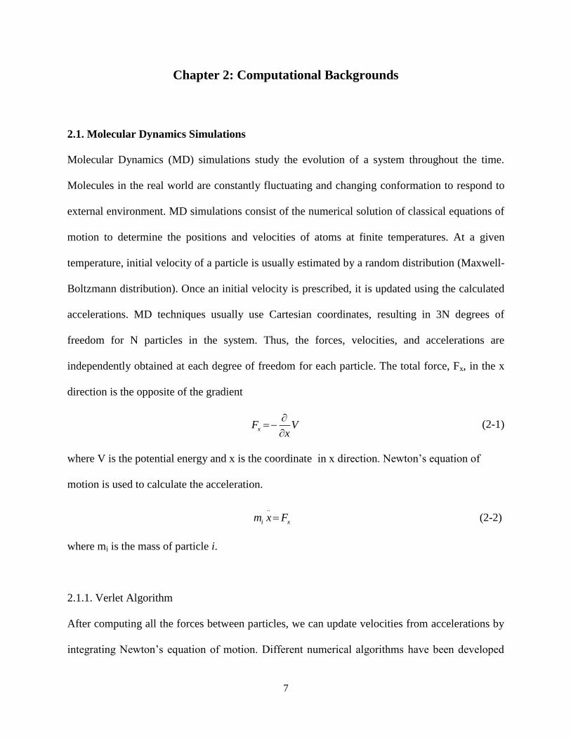
independently obtained at each degree of freedom for each particle. The total force, Fx, in the x
direction is the opposite of the gradient
xF V
x
(2-1)
where V is the potential energy and x is the coordinate in x direction. Newton’s equation of
motion is used to calculate the acceleration.
..
i xm x F (2-2)
where mi is the mass of particle i.
2.1.1. Verlet Algorithm
After computing all the forces between particles, we can update velocities from accelerations by
integrating Newton’s equation of motion. Different numerical algorithms have been developed
8
for integrating Newton’s equation of motion, such as Verlet algorithm (Verlet 1967), leap-frog
algorithm (Potter 1973), velocity-verlet algorithm (Swope 1982).
Verlet, initially used method of integrating the equations of motion using Taylor series expansion
which uses the positions r(t), accelerations a(t), and the previous position r(t-δt) to predict new
positions r(t+δt). Modifications to the basic Verlet algorithm have been proposed by Potter. In
this scheme, so called leap frog scheme, the current position r(t) and accelerations a(t) with the
midstep velocities v(t-(δt/2)) are used to obtain the next mid-step velocities v(t+(δt/2)). The
velocities leap over the positions and the positions leap over the velocities. Swope et al.
introduced the velocity-Verlet algorithm, because both the basic Verlet and leap frog algorithms
do not describe the velocities in a satisfactory manner. The velocity-Verlet algorithm needs to
store positions, accelerations, and velocities at the same time to minimize round-off error. This
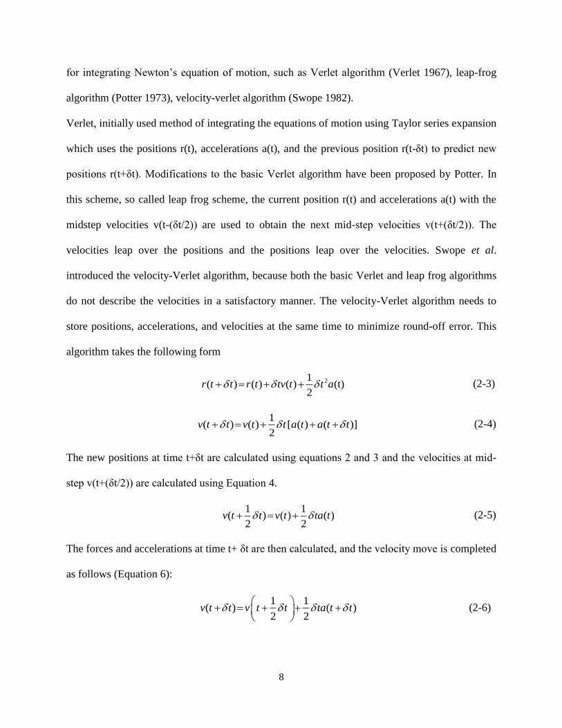
algorithm takes the following form
21( ) ( ) ( ) (t)
2r t t r t tv t t a (2-3)
1
( ) ( ) [ ( ) ( )]2
v t t v t t a t a t t (2-4)
The new positions at time t+δt are calculated using equations 2 and 3 and the velocities at mid-
step v(t+(δt/2)) are calculated using Equation 4.
) (1
)1
2) ((
2t v t tv t a t (2-5)
The forces and accelerations at time t+ δt are then calculated, and the velocity move is completed
as follows (Equation 6):
1 1
) ( )2
(2
t v t t ta t tv t
(2-6)
9
2.1.2. Ensembles
Ensemble is an assembly of all possible microstates, defined by given constraints. For example, a
simple way to create a thermodynamic ensemble is to maintain a constant total energy, volume,
and number of particles in a system to produce a microcanonical (NVE) ensemble of
conformations. In the same way, canonical (NVT) ensemble assembly of all states with fixed
number of particles, volume, and temperature and isobaric-isothermal (NPT) ensemble fixed
number of particles, pressure, and temperature. Once ensemble is formed, relative free energies,
average densities, and other thermodynamic properties can be calculated.
2.1.3. Energy Minimization
Energy minimization is typically performed by perturbing atoms in order to reduce the net force
applied to atoms by the force field potentials. Since a minimized structure usually has a well-
mannered geometry and rarely has large forces on any atom, it is preferred to start a molecular
dynamics simulation with a minimized structure. Energy minimization can be carried out in
Cartesian coordinates by optimizing in 3N-dimensional space where N is the number of particles
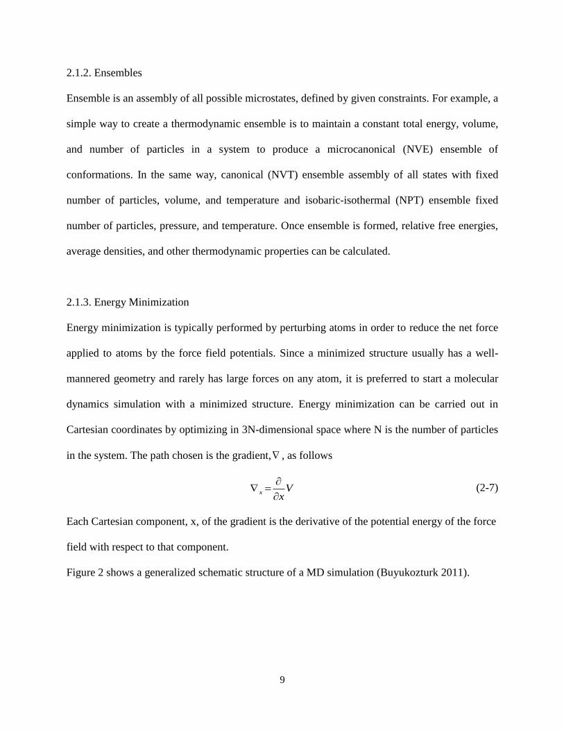
in the system. The path chosen is the gradient, , as follows
x V
x
(2-7)
Each Cartesian component, x, of the gradient is the derivative of the potential energy of the force
field with respect to that component.
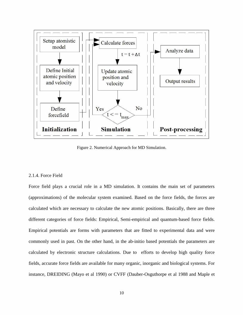
Figure 2 shows a generalized schematic structure of a MD simulation (Buyukozturk 2011).
10
Figure 2. Numerical Approach for MD Simulation.
2.1.4. Force Field
Force field plays a crucial role in a MD simulation. It contains the main set of parameters
(approximations) of the molecular system examined. Based on the force fields, the forces are
calculated which are necessary to calculate the new atomic positions. Basically, there are three
different categories of force fields: Empirical, Semi-empirical and quantum-based force fields.
Empirical potentials are forms with parameters that are fitted to experimental data and were
commonly used in past. On the other hand, in the ab-initio based potentials the parameters are
calculated by electronic structure calculations. Due to efforts to develop high quality force
fields, accurate force fields are available for many organic, inorganic and biological systems. For
instance, DREIDING (Mayo et al 1990) or CVFF (Dauber-Osguthorpe et al 1988 and Maple et
11
al 1988) are well-known generic force fields and CHARMM (Brooks et al 1983) or AMBER
(Weiner et al 1984 and Weiner et al 1986) are well developed force fields to describe biological
systems. The force field used in the all-atom MD simulations in this study is Condensed-Phased
Optimized Molecular Potential (COMPASS) developed by Sun et al 1998, which is explained in
detail in Chapter 3. In this section, we only mention the overall structure of all force field types.
The total energy is expressed by force field for a molecular system as a sum of valence (or
bonded) interactions and nonbonded interactions
ETotal = Evalence + Enonbonded (2-7)
The valence interactions can be broken down into bond stretch, bond angle bending, dihedral
angle torsion, and inversion term
Evalence = Ebond + Eangle + Etorsion + Einversion (2-8)
The first valence term in a force field is a bond stretch term. The simplest form for it is harmonic
bond potential:
2
0
1( )
2b bE K R R (2-9)
where R is the bond distance in units of Angstrom (A°), Ro is the equilibrium bond distance and
Kb is the force constant in unit of (kcal/mol)/A°2. In harmonic bond potential, the bond is
considered as a spring with equilibrium bond length of R0 and spring constant Kb. Also, there are
other forms for expressing stretch bond potential, which can also capture the R=∞ (interpreted as
a broken bond). Morse potential is one of the most famous potentials for this purpose:
0( ) 2
00
[ 1] ,2
R R bb
KE D e
D
(2-10)
12
R0 and Kb are the same as in harmonic bond potential. D0 is the bond energy in units of kcal/mol
and α is the Morse scaling parameter. The scaling parameter allows the bond energy to go to D0
for large R.
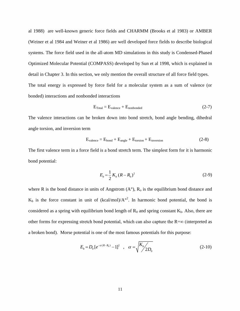
The second valence term in a force field is a bond angle bend as illustrated in Figure 3. The most
basic and common bond angle form is a harmonic potential
2
0
1( )
2aE K (2-11)
where θ, θ0 and Kθ are the bond angle, equilibrium bond angle and the force constant in units of
(kcal/mol)/A°2.
Figure 3. Bond Angle Bend.
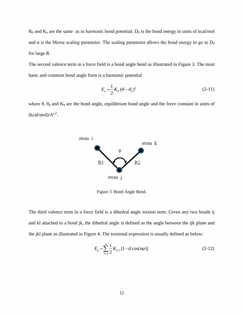
The third valence term in a force field is a dihedral angle torsion term. Given any two bonds ij
and kl attached to a bond jk, the dihedral angle is defined as the angle between the ijk plane and
the jkl plane as illustrated in Figure 4. The torsional expression is usually defined as below:
,
1
1[1 cos( )]
2
p
n
n
E K d n
(2-12)
13
where each Kθ,n is one half the rotational barrier in units of kcal/mol, n=1,2,3,4,5,6 is the
periodicity of the potential and d=±1 is the phase factor. For d=+1, the conformation is in the
minimum value while for the d=-1, it is in the maximum value.
Figure 4. Torsion Angle.
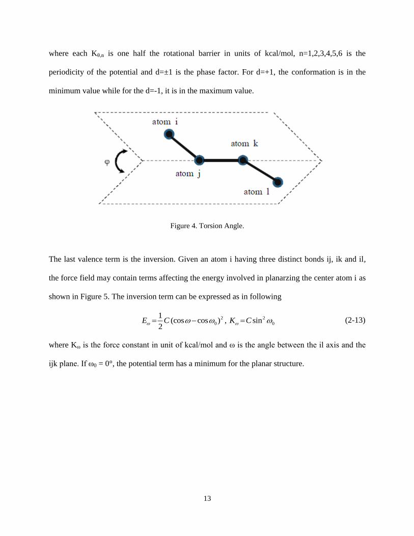
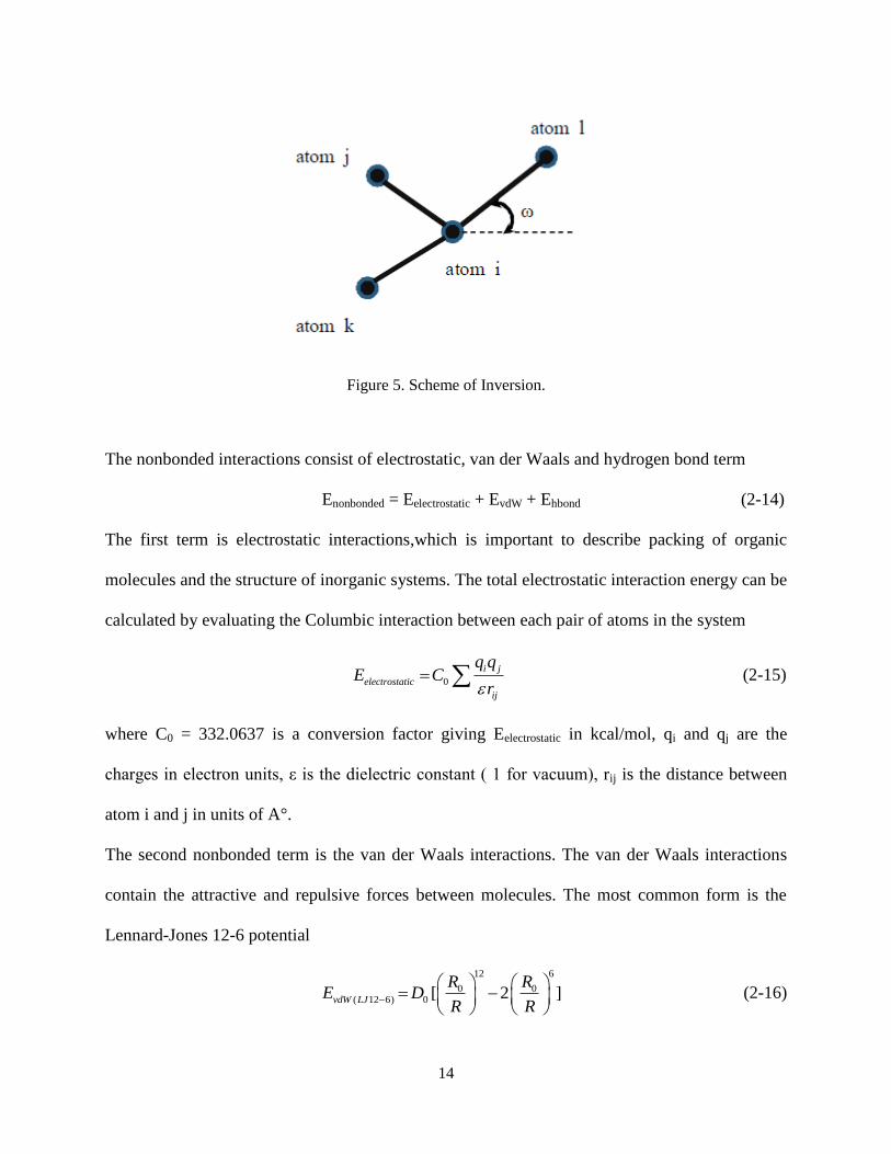
The last valence term is the inversion. Given an atom i having three distinct bonds ij, ik and il,
the force field may contain terms affecting the energy involved in planarzing the center atom i as
shown in Figure 5. The inversion term can be expressed as in following
2 2
0 0
1(cos cos ) , sin
2E C K C (2-13)
where Kω is the force constant in unit of kcal/mol and ω is the angle between the il axis and the
ijk plane. If ω0 = 0°, the potential term has a minimum for the planar structure.
14
Figure 5. Scheme of Inversion.
The nonbonded interactions consist of electrostatic, van der Waals and hydrogen bond term
Enonbonded = Eelectrostatic + EvdW + Ehbond (2-14)
The first term is electrostatic interactions,which is important to describe packing of organic
molecules and the structure of inorganic systems. The total electrostatic interaction energy can be
calculated by evaluating the Columbic interaction between each pair of atoms in the system
0
i j
electrostatic
ij
q qE C
r (2-15)
where C0 = 332.0637 is a conversion factor giving Eelectrostatic in kcal/mol, qi and qj are the
charges in electron units, ε is the dielectric constant ( 1 for vacuum), rij is the distance between
atom i and j in units of A°.
The second nonbonded term is the van der Waals interactions. The van der Waals interactions
contain the attractive and repulsive forces between molecules. The most common form is the
Lennard-Jones 12-6 potential
12 6
0 0( 12 6) 0 [ 2 ]vdW LJ
R RE D
R R
(2-16)
15
where D0 is well depth and R0 is the equilibrium distance (in A°). The main drawback of this
from is that it requires only two parameters, D0 and R0. For R<R0, the Lennard-Jones potential
may be too repulsive at short ranges. A more reasonable form, the exponential-6 potential and
Morse potential (Equations 16 and 17, respectively) allows three parameters to describe the
inner wall (short ranges) more realistically.
0
61
0(exp 6) 0
6 6exp
6 6
R
R
vdW
RE D
R
(2-17)
2
( ) 0
0
( 2 ) , exp 12
vdW Morse
RE D
R
(2-18)
The last nonboned term in a force field is H bond. Some force fields like CHARMM and
DREIDING use a hydrogen bond potential to describe the interaction between atoms involved in
hydrogen bonds. The general form of hydrogen bond is Lennard-Jones 10-12 potential, as
expressed below:
12 10
0 0( 12 10) 5 6hbond LJ
R RE D
R R
(2-19)
where D0 is the hydrogen bond strength in kcal/mol and R0 is equilibrium distance in A° (Lee
2011).
16
Chapter 3: Atomistic Modeling of Crosslinked Polymers
Crosslinked polymers are one of the main types of compounds that are usually consisted of an
epoxy group and a curing agent. They exhibit excellent properties, i.e. high modulus and fracture
strength, low creep and high-temperature resistance and thus widely used as coatings, adhesives,
composites, etc. In order to design and manipulate these properties, we need to gain a better
understanding of the molecular structure. MD simulations can shed light on the atomic structure
of the crosslinked polymers and how the macro properties are affected by the microstructure. For
this purpose, we need a crosslinking protocol that can be used to model the crosslinked
polymers. In this thesis, a crosslinking protocol is described in detail which is proposed by Wu
and Xu 2006.
This crosslinking algorithm is performed on a set of resin epoxies and the results are validated by
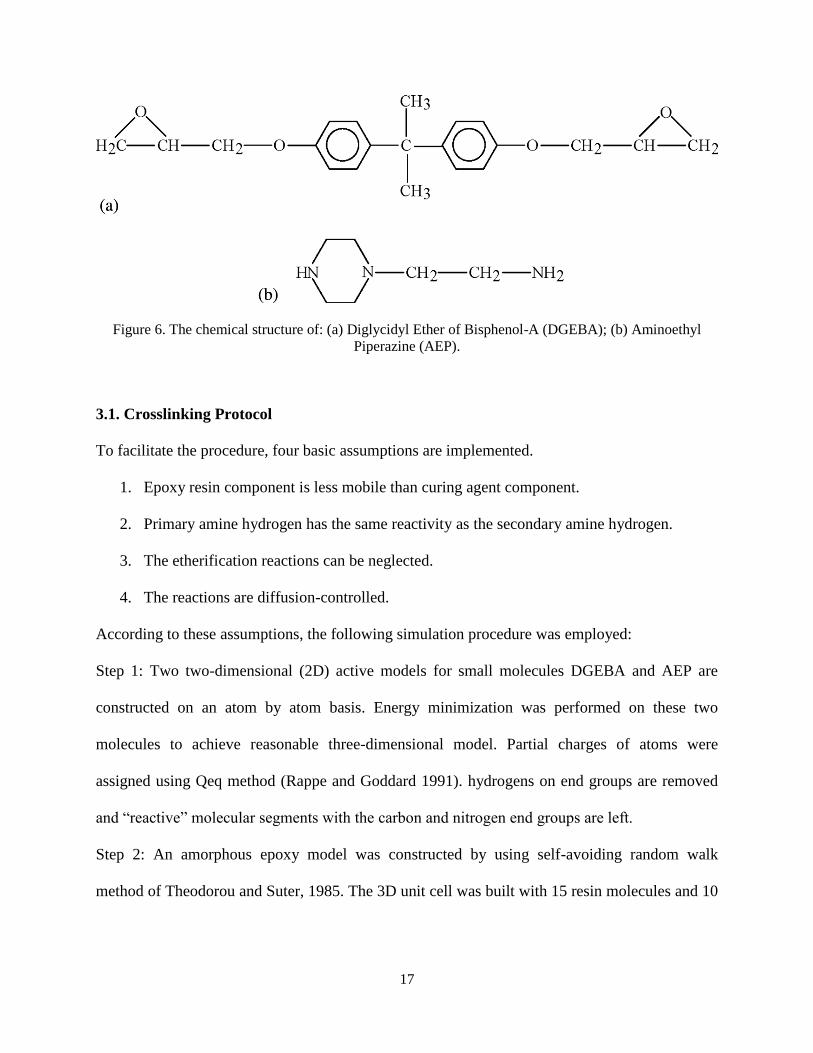
experiment. The epoxy system used in this study is based on Diglycidyl Ether of Bisphenol-A
(DGEBA), which is commercially known as EPON 828. The curing agent used with the epoxy
(DGEBA) is Aminoethyl Piperazine (AEP), commercially known as EPICURE 3200, as shown
in Figure 6.
17
Figure 6. The chemical structure of: (a) Diglycidyl Ether of Bisphenol-A (DGEBA); (b) Aminoethyl
Piperazine (AEP).
3.1. Crosslinking Protocol
To facilitate the procedure, four basic assumptions are implemented.
1. Epoxy resin component is less mobile than curing agent component.
2. Primary amine hydrogen has the same reactivity as the secondary amine hydrogen.
3. The etherification reactions can be neglected.
4. The reactions are diffusion-controlled.
According to these assumptions, the following simulation procedure was employed:
Step 1: Two two-dimensional (2D) active models for small molecules DGEBA and AEP are
constructed on an atom by atom basis. Energy minimization was performed on these two
molecules to achieve reasonable three-dimensional model. Partial charges of atoms were
assigned using Qeq method (Rappe and Goddard 1991). hydrogens on end groups are removed
and “reactive” molecular segments with the carbon and nitrogen end groups are left.
Step 2: An amorphous epoxy model was constructed by using self-avoiding random walk
method of Theodorou and Suter, 1985. The 3D unit cell was built with 15 resin molecules and 10
18
agents. The molecules were packed into the cell with a density of 1.16 g/cm3. Periodic Boundary
Conditions (PBC) are imposed to the system to eliminate the boundary effects.
Step 3: An energy minimization is performed for 1000 steps. Then a cyclic isothermal (NVT)
and isothermal-isobaric (NPT) is performed in the room temperature (298 K) to relax the initial
unit cell model. The resulting physical mixture was analyzed in order to identify the reactive
sites in close proximity. One of the reactive site’s carbons in DGEBAs was first chosen. Then a
search of nearby reactive site’s nitrogen in AEP is conducted. The reaction occurs between a pair
of such reactive sites when their distance is within a reaction cutoff distance of 4 A°.
Step 4: The temperature is raised to 500K and then the system is further cooled down by a rate of
100 K/ 100 ps. At each step, NVT and NPT dynamic simulations are performed. The time length
of both NVT and NPT simulations are 100ps. Then the system is checked for the distance
between the reactive sites and if they are closer than the cutoff distance, bonds are created.
Step 5: The cooling down process is repeated (Step 4) and at each step, the reactive site’s
distances are measured. This process is repeated until the temperature reaches the initial room
temperature. The time step for all the dynamic simulations are assumed as 1 fs.
Crosslinking protocol is then applied to the unit cell, elastic properties of the systems are studied
through a uniaxial deformation. The Young Modulus of the polymer was computed performing a
dynamic simulation, while applying a force of 0.5 kcal/mol/A. This force was exerted to the
system by applying a strain amplitude of 0.003 to the cell. Drieding (Mayo et al 1990) and
Condensed-Phased Optimized Molecular Potential (COMPASS) (Sun 1998) force-fields are
among the most common force-fields in simulations of epoxy polymers. They have been
previously used to study the mechanical properties of epoxy polymers (Wu and Xu 2006,
19
Grujicic et al 2007, Lu and Dunn 2010). Both force-fields were used in this study and the results
are presented and compared in the proceeding section.
3.2. Results
Molecular modeling of the polymer was performed by the methodology prescribed earlier. The
temperature of the system was initially raised to 500K and then, the system was cooled down to
room temperature with a rate of 100 K/20 ps. The cyclic NVT and NPT simulations were
performed at each cooling step, which helped the system to relax and reach to its minimum
energy configuration. Using this procedure, the bonds between the epoxy and the agents were
established through the reactive sites. COMPASS and DRIEDING force-fields have been
previously used to study mechanical properties of epoxies. In this study, we have used both
force-fields to model the DGEBA/AEP polymer and derive the mechanical properties. The
results in each case are compared with experimental values.
Once the molecules have been placed within the super cell, a series of alternating MD
simulations and static energy minimizations (molecular mechanics simulations) were used to
establish the equilibrated molecular structure at the corresponding density. The molecular
structures were gradually equilibrated to minimize any residual stresses in the model. After
constructing the super cell and a preliminary dynamics simulation, the second step was initiated
to simulate the crosslinking procedure. 20,000 time steps of NVT simulations were performed at
room temperature (298 K). Afterwards, the system’s temperature was gradually raised to 500 K.
It can be observed that after relaxing the system in the 500 K (third simulation) the Young’s
20
Modulus values decrease as illustrated in Figure 7. This process was repeated for the
temperatures at 400K and 300K.
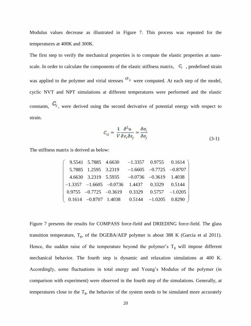
The first step to verify the mechanical properties is to compute the elastic properties at nano-
scale. In order to calculate the components of the elastic stiffness matrix, , predefined strain
was applied to the polymer and virial stresses were computed. At each step of the model,
cyclic NVT and NPT simulations at different temperatures were performed and the elastic
constants, , were derived using the second derivative of potential energy with respect to
strain.
(3-1)
The stiffness matrix is derived as below:
4.6630 1.3357 0.9755 0.16149.5541 5.7885
3.2319 1.6605 0.7725 0.87075.7885 1.2595
5.5935 0.0736 0.3619 1.40384.6630 3.2319
1.3357 1.6605 0.0736 1.4437 0.3329 0.5144
0.9755 0.7725 0.3619 0.3329 0.5757 1.0205
0.1614 0
.8707 1.4038 0.5144 1.0205 0.8290
Figure 7 presents the results for COMPASS force-field and DRIEDING force-field. The glass
transition temperature, Tg, of the DGEBA/AEP polymer is about 388 K (Garcia et al 2011).
Hence, the sudden raise of the temperature beyond the polymer’s Tg will impose different
mechanical behavior. The fourth step is dynamic and relaxation simulations at 400 K.
Accordingly, some fluctuations in total energy and Young’s Modulus of the polymer (in
comparison with experiment) were observed in the fourth step of the simulations. Generally, at
temperatures close to the Tg, the behavior of the system needs to be simulated more accurately
21
with a different approach. In terms of mechanical behavior, the material is in a transition state
which leads to these fluctuations. Hence, these fluctuations were expected and were not
considered in this study.
In the last step the temperature was set back to the room temperature. There is a remarkable
difference observed between the Young’s modulus in second and fifth step which were both
performed at the room temperature. This difference clearly shows the effect of the crosslinking
process in the mechanical behavior of the polymer, Figure 7.
Figure 7 present the computed Young’s modulus as a function of the simulations step for both
COMPASS and DREIDING force field. The DREIDING force field shows fewer fluctuations
but the results are significantly different from the experimental data. Meanwhile, the computed
Young’s modulus using the COMPASS force field approached to the experimental values as the
simulation progressed. It is also clear from these results that the DREIDING force field is not
suitable for modeling cross-linking process in the cross-linked epoxy studied here, since the
Young’s modulus does not significantly change as the simulation progresses.
Using COMPASS force field, the final computed Young Modulus is about 2.31 GPa. The
experimental data (Grujicic et al 2007) show the Young’s Modulus of DGEBA/AEP polymer is
in the range of 2.7-2.9 GPa. Hence, the suggested simulation process is capable of modeling the
mechanical properties of cross-linked polymers.
22
Figure 7. Variation of epoxy Young’s modulus as the simulations of curing process progresses using
Drieding and COMPASS force-fields. The thermal step for cross-linking is 100 K from 298 raised to 500
and cooled back to 298 again.
23
Chapter 4: All-Atom Molecular Dynamics Simulation
4.1. Introduction
Hydrogels are three-dimensionally crosslinked polymer networks that can absorb and retain large
amount of water, even up to thousands of theirs dry weight (Lowman et al 1999 and Hoffman
2012). They do not dissolve in water due to the presence of covalent bonds in the crosslinks
zones. Among different properties of hydrogels, we are interested in the mechanical properties.
Toughness and strength are required for many functional applications of gels.
Molecular Dynamics (MD) simulations have been employed to study various properties of
hydrogels including the equilibrated structure, mechanical properties, diffusivity of water and
ions. Jang et al. have studied mechanical properties of double network (DN) hydrogels. They
obtained stress-strain curves for DN hydrogels by applying uniaxial deformation up to 300%.
Lee et al. have studied the structure and mechanical properties of crosslinked hydrogels in both
blocky and random hydrogels. E. Chiessi et al. have studied dynamics of polymer and water in
hydrogels. Swelling of hydrogels is one of the most characteristic properties of hydrogels which
occurs in an aqueous solution by absorbing the solvent. This process is influenced by many
factors. J .Walter et al. have studied swelling behavior of hydrogels by proposing a realistic MD
model of hydrogels obtained by the experiments on freeze-dried hydrogel. Also, Y. Wu. et al.
focused on the diffusivity of water and ions in hydrogels. They have shown in their studies that
by increasing the crosslinking density, the diffusion coefficients decrease.
In this study, a novel method is applied to model the crosslinking process and studying
mechanical properties of hydrogels using molecular dynamics simulations. Stiffness matrices
24
and Elastic Modulus is calculated by applying a uniaxial strain to the system. The simulation
details are presented in the next section.
4.2. Simulation Details
4.2.1. Model Construction
The epoxy and curing agent used for this study are Polyethylene glycol diglycidyl ether
(PEGDGE) and the Jeffamine which is poly-oxy-alkylene-amines, respectively (see Figure 1).
The chemical structure of the PEGDGE and Jeffamine are built separately, and the end hydrogen
atoms are removed to provide reactive atom sites at the end groups, where the crosslinks will
form. The two polymer molecules are then packed into an amorphous unit cell which is
constructed using self-avoiding random walk method of Theodorou and Suter 1985. The unit cell
is built with a PEGDGE:Jeffamine ratio of 1 to 4, having a density of 1.086 g/cm3. Also, the
water molecule is packed into the system to reach different values for volume percent of water.
Five different systems are modeled containing 0, 20, 40, 60 and 80 wt%.
(a) (b)
Figure 8. Chemical structure of epoxy and curing agent with oxygen, nitrogen, carbon and hydrogen as
red, blue, grey and white respectively: (a) Polyethylene glycol diglycidyl ether (PEGDGE); (b)
polyoxyalkyleneamine (Jeffamine).
25
4.2.2. Crosslinking process
Conventional MD is not capable of modeling the crosslinking process which involves formation
and breaking of bonds. On the other hand, with the present computational resources,
sophisticated electronic structure calculation methods, such as ab-initio method, are very costly
and impractical, if not impossible, for macromolecules (e.g. polymers) and large systems. New
statistical methods have therefore been developed that allow for such calculations in a more
tractable way. The method developed by Wu and Xu et al 2006, is an example of such methods.
The main simplifying hypothesis in this technique is that it considers same reactivity for all the
end groups. The charge distribution is calculated using QEq method (Rappe and Goddard, 1991).
The process is modeled through cyclic canonical (NVT) and isothermal-isobaric (NPT)
ensembles. First a geometry optimization and energy minimization is performed in the room
temperature (298 K). Next, the system’s temperature is raised to 358K. The system is then
cooled down step by step at a rate of 10K/50ps. In each step, after the completion of NVT and
NPT simulations, the proximity of reactive sites are examined and if they are within a radius of 2
A° from each other, bonds are created. This process is repeated until the system reaches the
initial temperature. Nose-Hoover and Andersen algorithms are used as thermostat and barostat,
respectively.
4.2.3. Force field and simulation parameters
A crucial point in atomistic simulations is choosing a forcefield that result in an accurate enough
approximation of the potential energy hypersurface in which the nuclei moves. The potential
energy can be described as follows:
(4 1) total valence cross term non bondedE E E E
26
The valence energy consists of the bond-stretching term, bending energy and the four body terms
including a dihedral bond-torsion angle term and an inversion (out-of plane interaction) term:
4 2valence stretching bendeing dihedral torsion inversionE E E E E
The cross-term accounts for the energy changes induced by the change in the bond length and the
angle changes in the surrounding atoms as illustrated in the equation 3:
_ _
cross term bond bond angle angle bond angle end bond torsion middle bond torsion
angle torsion angle angle to
E E E E E E
E E 4 3
rsion
The last term in the Eq. 1 (the non-bonded term) consists of Inter and Intra-molecular
interactions, including hydrogen bonds (H-bonds), van der Waals interactions which are the
induced dipole-dipole interactions (also named as London forces) and finally, the Coulomb
interactions which account for electrostatic interactions.
4 4non bonded vdW Coulomb H bondE E E E
The condensed-phased optimized molecular potential (COMPASS) which has proved to be a
promising force field for organic and inorganic systems, is used in this study (Sun 1998, Sun et
al 1998 and Grujicic et al 2007). It is well parametrized for non-bonded interactions which
makes it a good fit for long chain molecules like biomaterials or polymers and systems where the
vdW is the governing interaction (Lu and Dunn 2010, Salahshoor and Rahbar 2012). The
COMPASS force field uses the following expressions for various components of the potential
energy:
27
'
2 3 4
2 0 3 0 4 0
2 3 4
2 0 3 0 4 0
0 0 0
1 1 2 2 3 3
2
'
0
[ ( ) ( ) ( ) ] (4 5)
[ ( ) ( ) ( ) ] (4 6)
[ [1 cos( )] [1 cos(2 )] [1 cos(3 )]] (4 7)
(4 8)
( )(
bond
b
angle
torsion
oop x
x
bond bond bb
E K b b K b b K b b
E H H H
E V V V
E K
E F b b b
'
'
'
'
'
0
' '
0 0
0 0
_ 0 1 2 3
' '
_ 0 1 2
) (4 9)
( )( ) (4 10)
( )( ) (4 11)
( )[ cos cos2 cos3 ] (4 12)
( )[ cos cos
b b
angle angle
bond angle b
b
end bond torsion b
b
middle bond torsion b
b
E F
E F b b
E F b b V V V
E F b b F F
'
'
'
3
0 1 2 3
' '
0 0
9 6
2 cos3 ] (4 13)
( ) [ cos cos2 cos3 ] (4 14)
cos ( )( ) (4 15)
(4 16)
[ ] (4 17)
b
angle torsion
angle angle torsion
i j
Coulumb
i j ij
ij ij
vdW
i j ij ij
F
E F V V V
E K
q qE
r
A BE
r r
Where b, θ, Ф and χ are the bond length, bond-angle, dihedral torsion angle and the inversion or
out of plane angle respectively. Also, q is the atomic charge, ε is dielectric constant and rij is the
28
interatomic distance between the atoms i and j. Finally, b0, Ki (i=2-4), θ0, Hi (i=2-4), Фi0 (i=1-3),
Vi (i=1-3),' ' ' '
' '
0 0, , , , , , , ( 1 3), , ,b b i ijbb bF b F F F F F i F K A
and Bij are the system
dependent parameters implemented in the Material Studio 6.0 software package , which is used
in this study.
4.3. Results and Discussion
4.3.1. Crosslinking process
As mentioned before, the crosslinking process is performed by creating reactive sites and cyclic
NVT and NPT dynamics simulations.To this end, H-atoms are removed from NJeff (end nitrogen
atoms in the Jeffamine) and CPEGDGE (end carbon atoms in the PEGDGE). These are shown in
blue and grey in Fig 1. Figure 2 shows the hydrogel structure before and after crosslinking. In
order to mimic the natural crosslinking process, a probability of 70% is imposed when creating
bonds. In other words, about 70 percent of crosslinks are created. This is clearly seen in the
Figure2. (b) where some NJeff atoms are still not connected to any carbon atoms of PEGDGE.
29
(a) (b)
Figure 9. The hydrogel initial model without water: (a) before crosslinking; (b) after crosslinking.
The distribution of NJeff and CPEGDGE atoms before and after the crosslinking provides a better
insight into the process. This is analyzed by radial distribution function (RDF). ( )A Bg r is the
probability density of finding atoms A and B at a distance r averaged over the equilibrium
trajectory, so that:
2
( ) ( ) ( ) (4 18)4
B BA B
n Ng r
r dr V
where Bn is the number of B particles located at a distance r in a shell of thickness dr from A
particle, NB is the total number of B particles in the system, and V is the total volume of the
system. ( )
Jeff PEGDGEN Cg r characterizes the relative configuration of N and C atoms in the curing
agent and epoxy quantitatively. Figure 3 shows the RDF of the system before and after the
crosslinking simulations. Basically, the two RDFs are for a pair of atoms once in two different
30
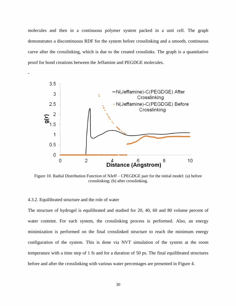
molecules and then in a continuous polymer system packed in a unit cell. The graph
demonstrates a discontinuous RDF for the system before crosslinking and a smooth, continuous
curve after the crosslinking, which is due to the created crosslinks. The graph is a quantitative
proof for bond creations between the Jeffamine and PEGDGE molecules.
-
Figure 10. Radial Distribution Function of NJeff – CPEGDGE pair for the initial model: (a) before
crosslinking; (b) after crosslinking.
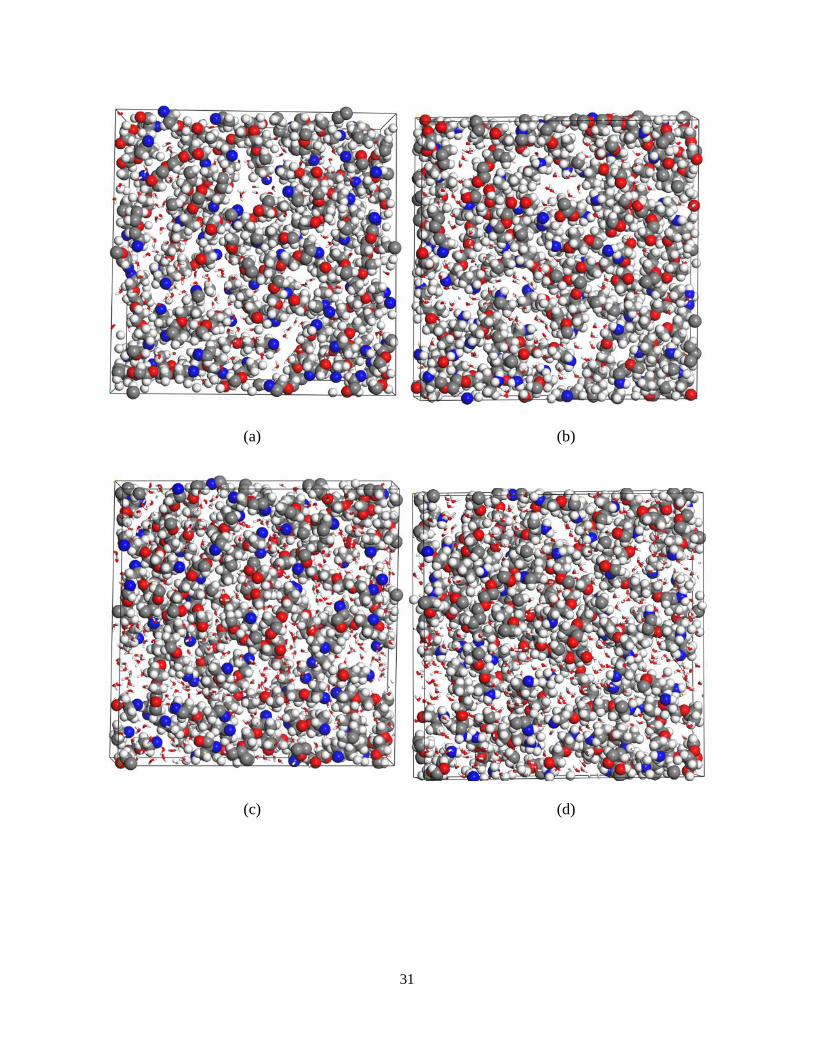
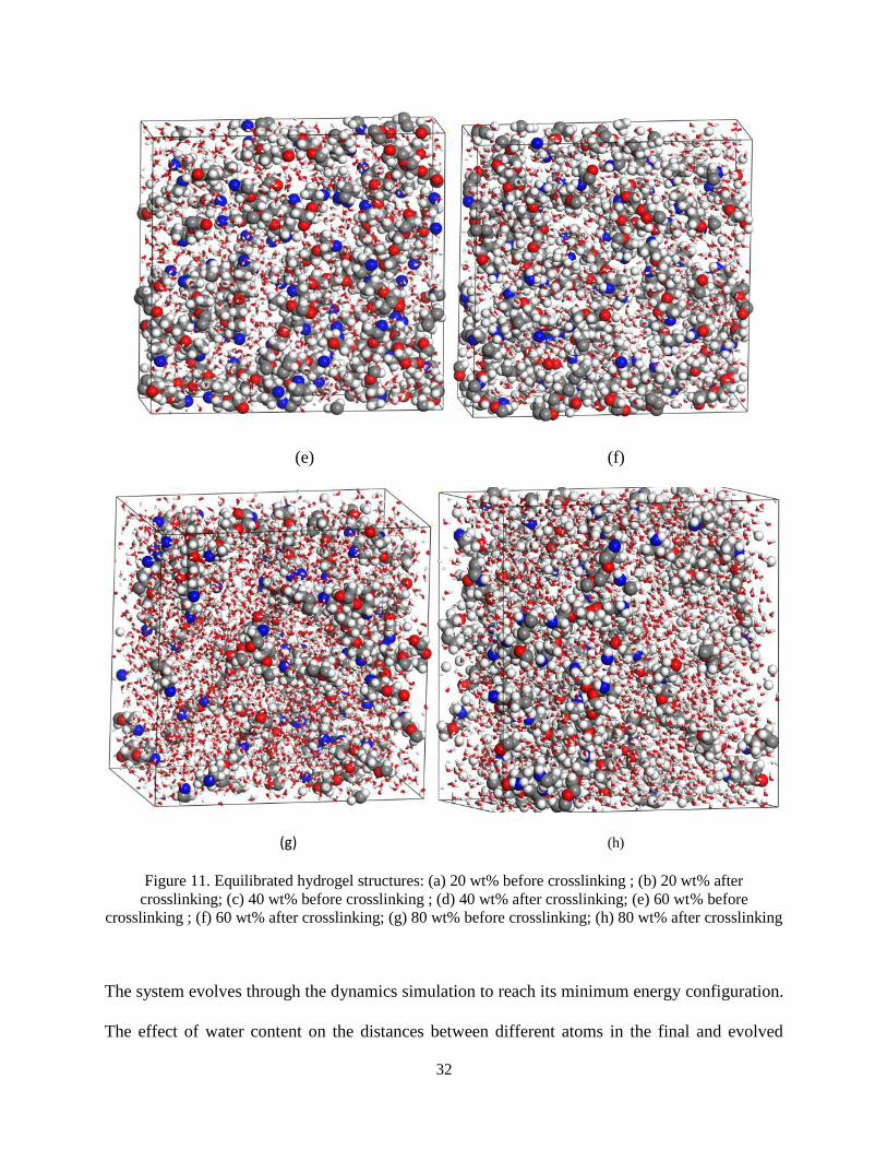
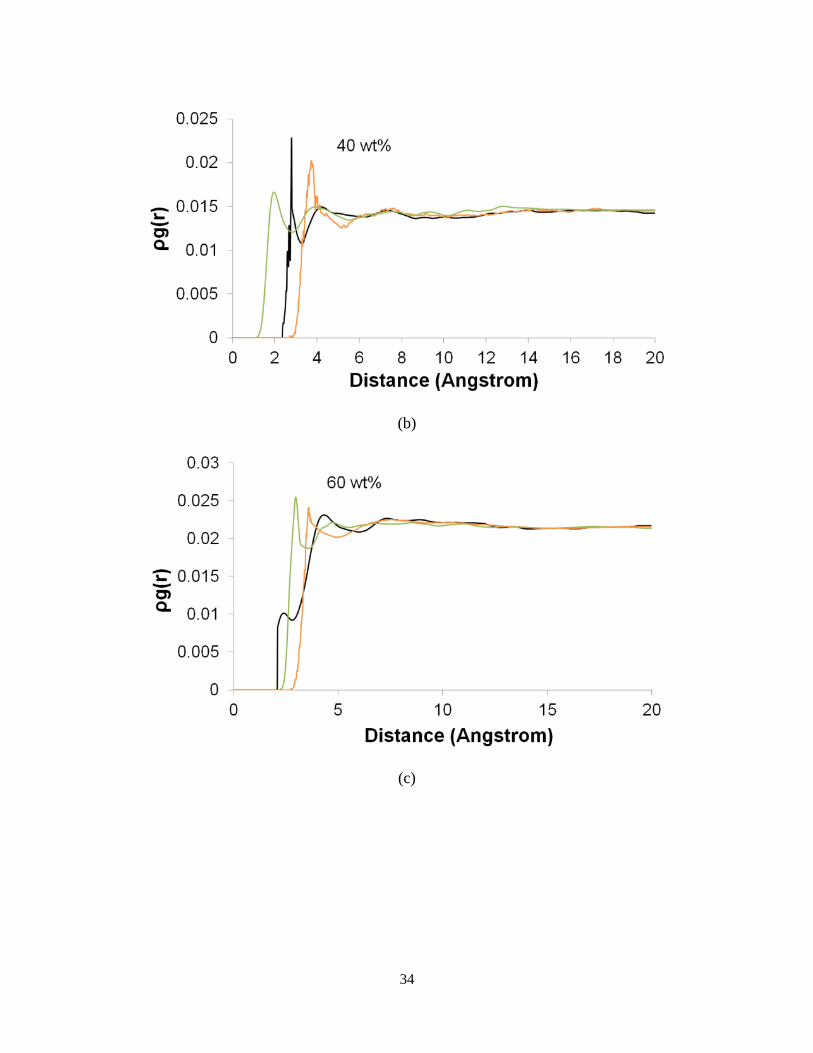
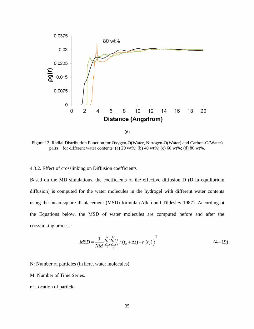
4.3.2. Equilibrated structure and the role of water
The structure of hydrogel is equilibrated and studied for 20, 40, 60 and 80 volume percent of
water contetnt. For each system, the crosslinking process is performed. Also, an energy
minimization is performed on the final crosslinked structure to reach the minimum energy
configuration of the system. This is done via NVT simulation of the system at the room
temperature with a time step of 1 fs and for a duration of 50 ps. The final equilibrated structures
before and after the crosslinking with various water percentages are presented in Figure 4.
31
(a) (b)
(c) (d)
32
(e) (f)
(g) (h)
Figure 11. Equilibrated hydrogel structures: (a) 20 wt% before crosslinking ; (b) 20 wt% after
crosslinking; (c) 40 wt% before crosslinking ; (d) 40 wt% after crosslinking; (e) 60 wt% before
crosslinking ; (f) 60 wt% after crosslinking; (g) 80 wt% before crosslinking; (h) 80 wt% after crosslinking
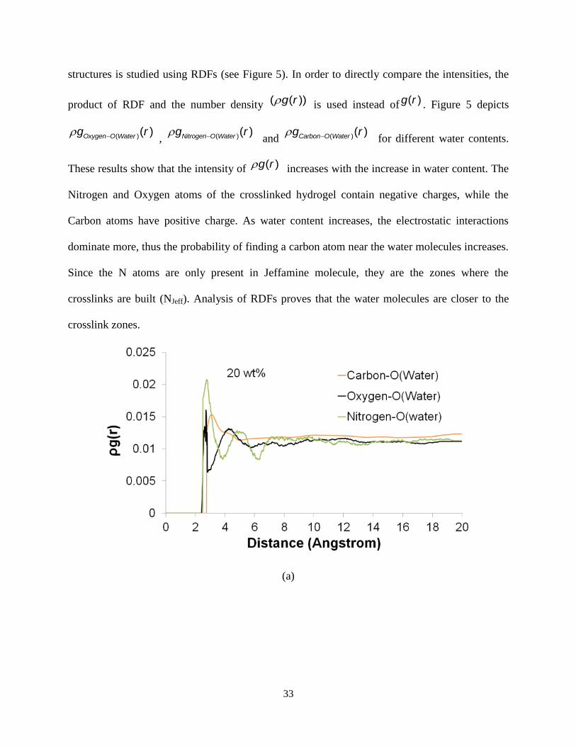
The system evolves through the dynamics simulation to reach its minimum energy configuration.
The effect of water content on the distances between different atoms in the final and evolved
33
structures is studied using RDFs (see Figure 5). In order to directly compare the intensities, the
product of RDF and the number density ( ( ))g r is used instead of ( )g r . Figure 5 depicts
( )( )Oxygen O Waterg r , ( )( )Nitrogen O Waterg r
and ( )( )Carbon O Waterg r for different water contents.
These results show that the intensity of ( )g r increases with the increase in water content. The
Nitrogen and Oxygen atoms of the crosslinked hydrogel contain negative charges, while the
Carbon atoms have positive charge. As water content increases, the electrostatic interactions
dominate more, thus the probability of finding a carbon atom near the water molecules increases.
Since the N atoms are only present in Jeffamine molecule, they are the zones where the
crosslinks are built (NJeff). Analysis of RDFs proves that the water molecules are closer to the
crosslink zones.
(a)
34
(b)
(c)
35
(d)
Figure 12. Radial Distribution Function for Oxygen-O(Water, Nitrogen-O(Water) and Carbon-O(Water)
pairs for different water contents: (a) 20 wt%; (b) 40 wt%; (c) 60 wt%; (d) 80 wt%.
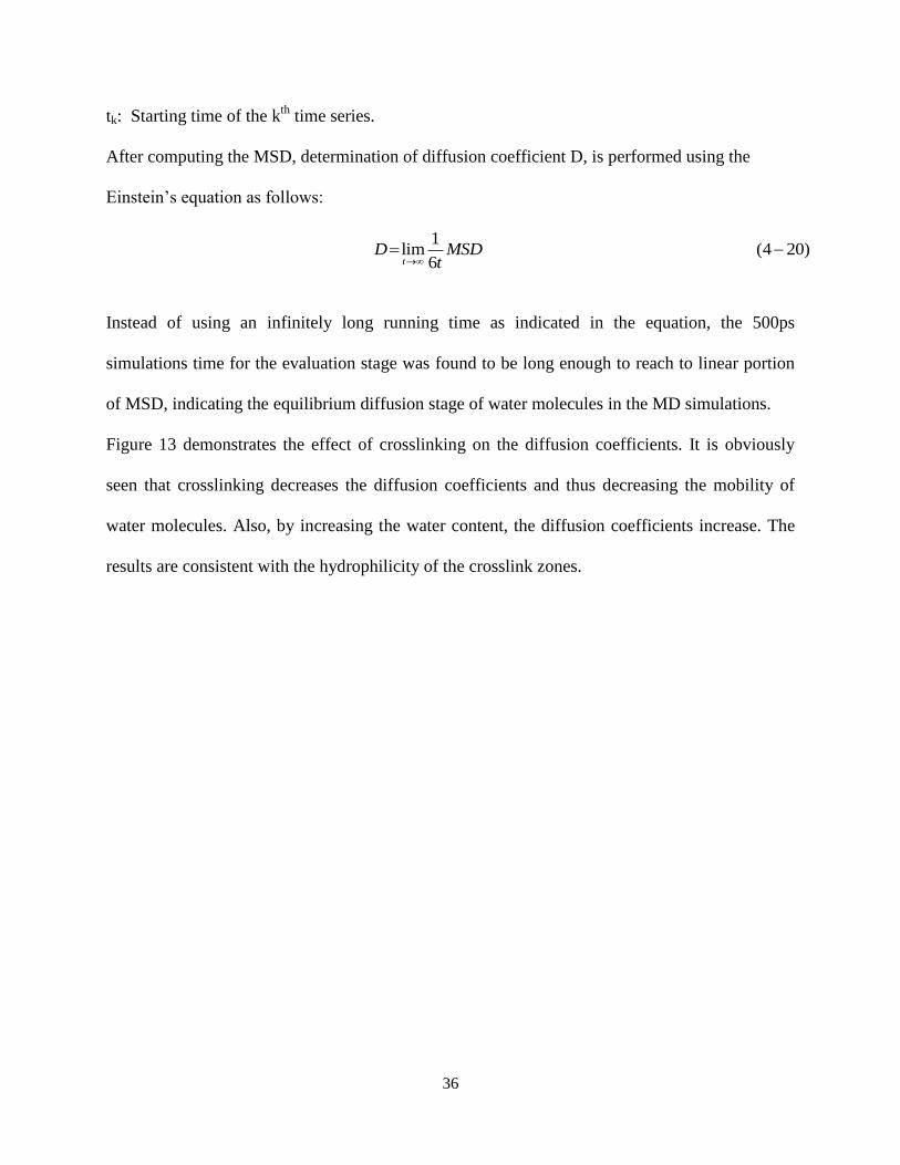
4.3.2. Effect of crosslinking on Diffusion coefficients
Based on the MD simulations, the coefficients of the effective diffusion D (D in equilibrium
diffusion) is computed for the water molecules in the hydrogel with different water contents
using the mean-square displacement (MSD) formula (Allen and Tildesley 1987). According ot
the Equations below, the MSD of water molecules are computed before and after the
crosslinking process:
21
( ) ( ) (4 19)N M
i k i k
i k
MSD r t t r tNM
N: Number of particles (in here, water molecules)
M: Number of Time Series.
ri: Location of particle.
36
tk: Starting time of the kth
time series.
After computing the MSD, determination of diffusion coefficient D, is performed using the
Einstein’s equation as follows:
1lim (4 20)
6tD MSD
t
Instead of using an infinitely long running time as indicated in the equation, the 500ps
simulations time for the evaluation stage was found to be long enough to reach to linear portion
of MSD, indicating the equilibrium diffusion stage of water molecules in the MD simulations.
Figure 13 demonstrates the effect of crosslinking on the diffusion coefficients. It is obviously
seen that crosslinking decreases the diffusion coefficients and thus decreasing the mobility of
water molecules. Also, by increasing the water content, the diffusion coefficients increase. The
results are consistent with the hydrophilicity of the crosslink zones.
37
Figure 13. Diffusion coefficients for water molecules in different water contents, both before and after
crosslinking.
4.3.3. Elastic Properties of hydrogels
Mechanical properties of hydrogel are studied by applying a predefined strain to unit cell. For a
uniaxial testing, a total strain amplitude of 0.003 is applied to the simulation box which is
enforced equally at each simulation step (every 1 fs). The stress is calculated from the uniaxial
test in the x-direction using the virial relation:
( )
1(4 21)
2ij ij iji
j i
r f
where i is a small volume around an atom i. The interatomic force fij applied on atom i by atom
j is:
38
( )(4 22)
ij ij
ij
ij ij
E r rf
r r
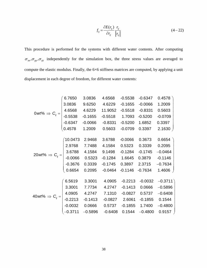
This procedure is performed for the systems with different water contents. After computing
, ,xx yy zz independently for the simulation box, the three stress values are averaged to
compute the elastic modulus. Finally, the 6×6 stiffness matrices are computed, by applying a unit
displacement in each degree of freedom, for different water contents:
6.7650 3.0836 4.6568 -0.5538 -0.6347
3.0836 9.6250 4.6229 -0.1655 -0.0066
4.6568 4.6229 11.9052 -0.5518 -0.83310 %
-0.5538 -0.1655 -0.5518 1.7093 -0.52
-0.6347 -0.0066 -0.8331 -0.5200
0.4578 1.2009 0.5603 -0.0709
ijwt C
0.4578
1.2009
0.5603
00 -0.0709
1.6852 0.3397
0.3397 2.1630
10.0473 2.9468 3.6788 -0.0066 0.3673
2.9768 7.7488 4.1584 0.5323 0.3339
3.6788 4.1584 9.1498 -0.1284 -0.174520 %
-0.0066 0.5323 -0.1284 1.6645 0.3879
-0.3676 0.3339 -0.1745 0.3897 2.3715
0.6654 0.2095 -0.0464 -0.1146
ijwt C
0.6654
0.2095
0.0464
-0.1146
0.7634
-0.7634 1.4606
6.5619 3.3001 4.0905 -0.2213 -0.0032
3.3001 7.7734 4.2747 -0.1413 0.0666
4.0905 4.2747 7.1310 -0.0827 0.573740 %
-0.2213 -0.1413 -0.0827 2.6061 -0.1855
-0.0032 0.0666 0.5737 -0.1855 1.740
0.3711 0.5896 -0.6408 0.1544
ijwt C
0.3711
0.5896
0.6408
0.1544
0 0.4800
0.4800 0.9157
39
5.7631 3.4711 3.3436 -0.0054 -0.1865
3.4711 4.7573 3.8203 -0.0708 -0.4171
3.3436 3.8203 6.9301 -0.2693 0.013260 %
-0.0054 -0.0708 0.2693 1.5602 -0.2298
-0.1865 -0.4171 0.0132 -0.2298 1.878
0.1339 0.3931 -0.1272 0.1333
ijwt C
0.1339
0.3931
0.1272
0.1333
8 0.3903
0.3903 2.4970
4.9663 4.5360 3.3063 0.3025 0.6299
4.5360 6.5612 4.6907 -0.6374 0.1067
3.3063 4.6907 5.7067 -0.0107 0.687880 %
0.3025 -0.6374 0.0107 1.6099 0.4820
0.6299 0.1067 0.6878 0.4820 0.7627
0.1029 0.2596 0.6421 0.2120 0.9780
ijwt C
0.1029
0.2596
0.6421
0.2120
0.9780
0.5030
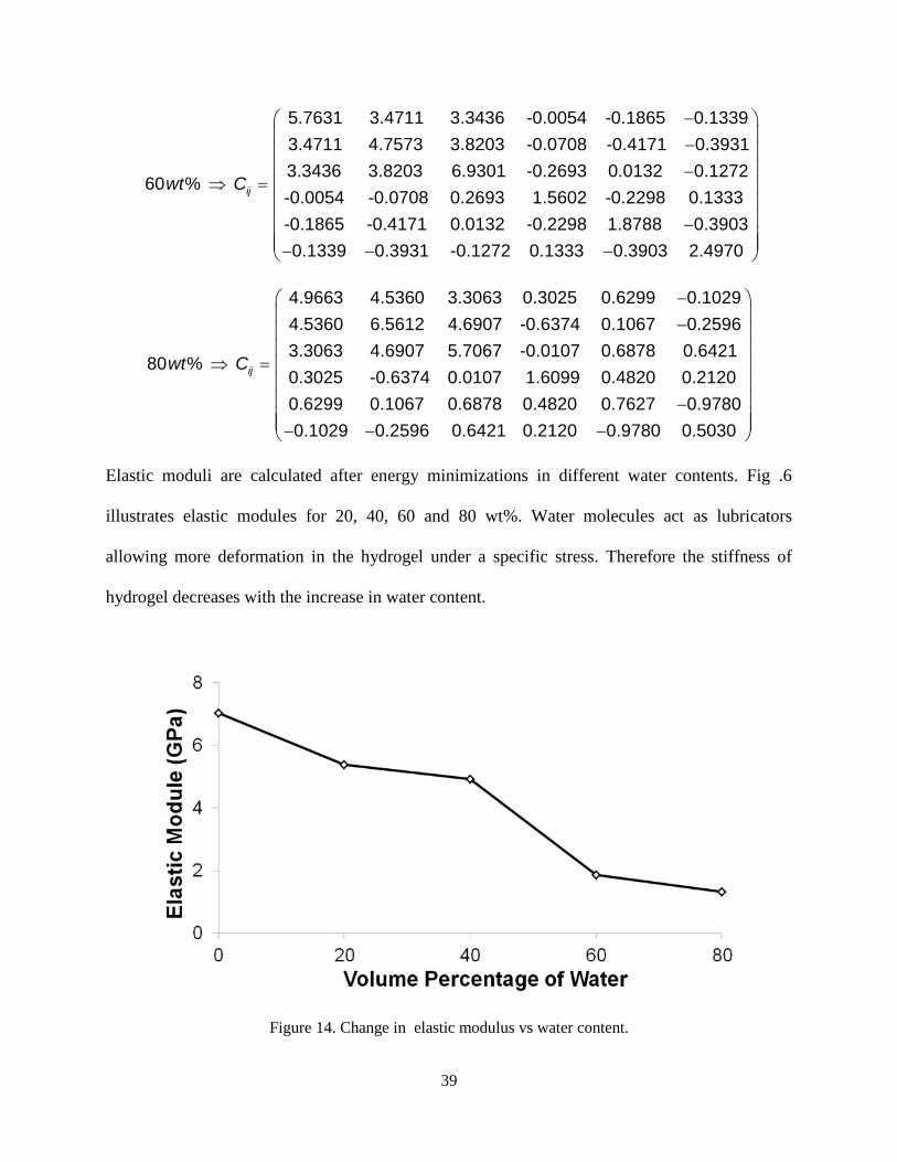
Elastic moduli are calculated after energy minimizations in different water contents. Fig .6
illustrates elastic modules for 20, 40, 60 and 80 wt%. Water molecules act as lubricators
allowing more deformation in the hydrogel under a specific stress. Therefore the stiffness of
hydrogel decreases with the increase in water content.
Figure 14. Change in elastic modulus vs water content.
40
4.4. Conclusion
Molecular dynamic simulation is used to study the effect of water on the equilibrated structure
and mechanical properties of crosslinked hydrogel. The hydrogel consisted of Polyethylene
glycol diglycidyl ether (PEGDGE) as epoxy and the Jeffamine which is poly-oxy-alkylene-
amines as curing agent. Different water contents (from 0 to 80 wt%) are examined. COMPASS
forcefield is employed for the simulations. Radial distribution functions, calculated for systems
with various water contents, indicate that the crosslinks are more hydrophilic within the hydrogel
structure. Mechanical properties are studied by applying strain to the system and the stiffness
matrices and elastic modulus are calculated for different water percentages. The results show that
the elastic modulus decreases by increasing the water content.
41
Chapter 5: Coarse-Grained model of Hydrogel
5.1. Introduction
The use of coarse grained (CG) models in a variety of simulation techniques has proven to be a
valuable tool to probe the time and length scales of systems beyond what is feasible with
traditional all atom (AA) models. Using all-atom methods, long simulations are very costly and
even close to impossible and they limit us to small length and especially time scales. A
promising strategy to overcome these limitations is to decrease number of degrees of freedom by
grouping atoms into pseudoatoms (or particles) referred to as beads (Gautieri et al 2010). This
represents the basis of the so-called coarse-grained approach, where, starting at the nanoscale, it
is possible to derive parameters for higher hierarchical levels, up to the macroscale by
systematically feeding information from smaller, more accurate to larger, coarser levels. Coarse-
Graining models were initiated for modeling huge biomolecules (Marrink et al, 2007).
Among different CG models, MARTINI coarse-grained model, developed by Marrink and co-
workers is used in this study. The MARTINI model provides suitable level of coarse-graining, as
it retains information about the chemistry. In the following section, the MARTINI approach for
the CG modeling is described.
5.2. MARTINI Model
5.2.1. Interaction Sites
The general mapping rule is that four heavy atoms (that is non-hydrogen atoms) are grouped
together into one bead, i.e. on average four heavy atoms are represented by a single interaction

42
center. For ring structures a different mapping is introduced, as will be explained below. In order
to keep the model simple, we still consider only four main types of interaction sites: polar (P),
nonpolar (N), apolar (C), and charged (Q). Each particle type has a number of subtypes, which
allow for a more accurate representation of the chemical nature of the underlying atomic
structure. Within a main type, subtypes are either distinguished by a letter denoting the
hydrogen-bonding capabilities (d=donor, a=acceptor, da=both, 0=none), or by a number
indicating the degree of polarity (from 1, low polarity, to 5, high polarity).
5.2.2. Bonded and Nonbonded Interactions
The form of the nonbonded interactions is the Lennard-Jones 12-6 potential energy function. In
addition to the LJ interaction, charged groups bear a full charge qi,j interacting via a shifted
Coulombic potential energy function:
0
( ) (5 1)4
i j
el
r
q qU r
r
with relative dielectric constant εr=15 for explicit screening.
Among bonded interactions, the form for the bond stretch is weak harmonic potential with an
equilibrium distance Rbond = σ = 0.47 nm and a force constant of Kbond= 1250 kJ mol-1
nm-2
. The
LJ interaction is excluded between bonded particles, because they are on average somewhat
closer to each other than neighboring nonbonded particles.
Also for bending potential, weak harmonic potential of the cosine type is used. Again, a set of
parameters are defined for this form. Also for most of linear chainlike molecules, a standard
43
force constant of Kangle= 25 kJ mol-1
with an equilibrium bond angle θ0 = 180° is the best initial
choice.
Basically, the force graining recipe consists of three steps:
1. Mapping onto CG representation: The first step is to divide the molecule into small
chemical building blocks, ideally of four heavy atoms each. Because most molecules
cannot be entirely mapped onto groups of four heavy atoms, however, some groups will
represent a smaller or larger number of atoms. There are different strategies for
modulation of building blocks, especially for certain compounds like those having ring
structures, described in Marrink et al. 2007.
2. Selecting bonded interactions: For most molecules the use of a standard bond length
(0.47 nm) and force constant of Kbond = 1250 kJ mol-1
nm-2
seems to work well. Ring
structures needs additional adjusting. Also, the values defined before for the bending
parameters are also working for most molecules.
3. Optimization: Since, coarse graining procedure does not lead to a unique assignment of
particle types and bonded interactions, the structure should be optimized. Validating the
results with the all-atom model is also popular.
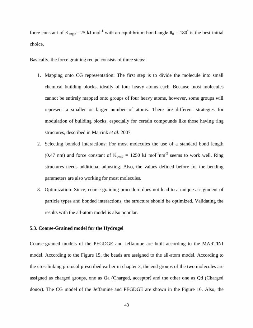
5.3. Coarse-Grained model for the Hydrogel
Coarse-grained models of the PEGDGE and Jeffamine are built according to the MARTINI
model. According to the Figure 15, the beads are assigned to the all-atom model. According to
the crosslinking protocol prescribed earlier in chapter 3, the end groups of the two molecules are
assigned as charged groups, one as Qa (Charged, acceptor) and the other one as Qd (Charged
donor). The CG model of the Jeffamine and PEGDGE are shown in the Figure 16. Also, the
44
water molecules are assigned as one bead. Since, water is highly polar molecules, it is assigned
as type P4 (Very Polar).
(a)
(b)
Figure 15. Coarse-Grain model for: (a) Jefffamine. (b) PEGDGE. The Nitrogen, Oxygen, Carbon and
Hydrogen atoms are shown in blue, red, grey and white, respectively.
45
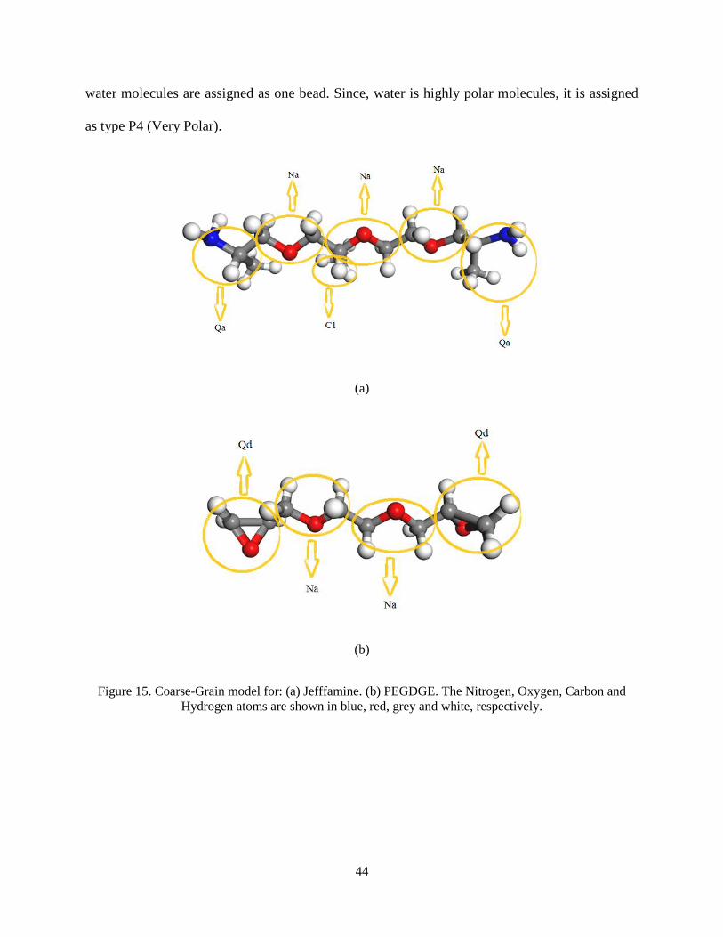
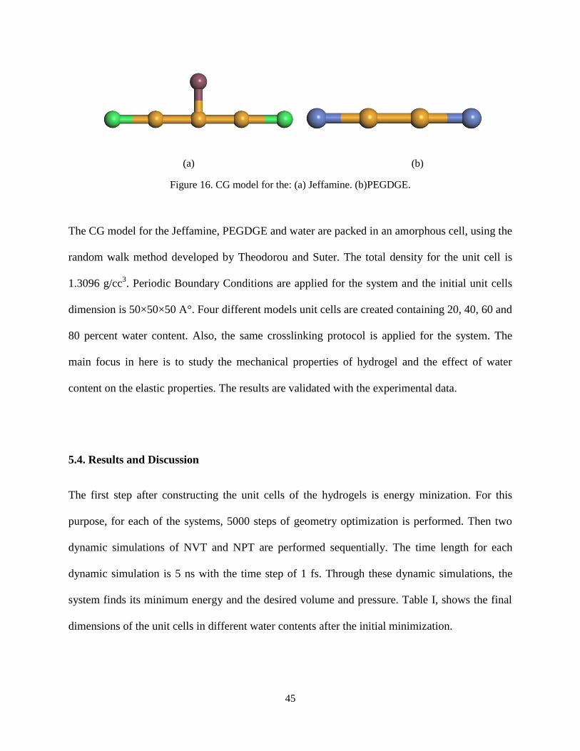
(a) (b)
Figure 16. CG model for the: (a) Jeffamine. (b)PEGDGE.
The CG model for the Jeffamine, PEGDGE and water are packed in an amorphous cell, using the
random walk method developed by Theodorou and Suter. The total density for the unit cell is
1.3096 g/cc3. Periodic Boundary Conditions are applied for the system and the initial unit cells
dimension is 50×50×50 A°. Four different models unit cells are created containing 20, 40, 60 and
80 percent water content. Also, the same crosslinking protocol is applied for the system. The
main focus in here is to study the mechanical properties of hydrogel and the effect of water
content on the elastic properties. The results are validated with the experimental data.
5.4. Results and Discussion
The first step after constructing the unit cells of the hydrogels is energy minization. For this
purpose, for each of the systems, 5000 steps of geometry optimization is performed. Then two
dynamic simulations of NVT and NPT are performed sequentially. The time length for each
dynamic simulation is 5 ns with the time step of 1 fs. Through these dynamic simulations, the
system finds its minimum energy and the desired volume and pressure. Table I, shows the final
dimensions of the unit cells in different water contents after the initial minimization.
46
Table 5-1. Cell dimenstions, Before and after the initial 10 ns minimizaion.
Water Content
(%)
Initial Dimension (A°)
Final Dimension After the
minimizations (A°)
20 50×50×50 63.99×63.99×63.99
40 50×50×50 68.58×68.58×68.58
60 50×50×50 72.54×72.54×72.54
80 50×50×50 76.61×76.61×76.61
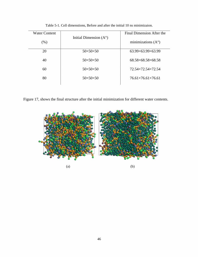
Figure 17, shows the final structure after the initial minimization for different water contents.
(a) (b)
47
(c) (d)
Figure 17. The structure after minimizations: (a). 20wt%, (b). 40wt%, (c). 60wt%, (d). 80wt%.
After the optimization and minimization steps, shear strain is applied to the system. The shear is
applied to the system step by step with a rate of 1e-5, through NPT dynamic simulations. Each
NPT simulation (applying shear) is performed within 4 ns with the time step of 10 fs. The
Berendsen algorithm is chosen for the thermostat and barostat. In order to optimize and stabilize
the pressure, each shear simulation is followed by a 1 ns dynamic NVT simulation.
0
2
4
6
8
10
0 0.1 0.2 0.3 0.4
Sh
ear
Str
ess
(MP
a)
Shear Strain
20 wt%
48
(a)
(b)
(c)
0
2
4
6
8
10
0 0.1 0.2 0.3 0.4
Sh
ear
Str
ess
(MP
a)
Shear Strain
40 wt%
0
1
2
3
4
5
6
0 0.1 0.2 0.3
Sh
ear
Str
ess
(MP
a)
Shear Strain
60 wt%
49
(d)
Figure 18. Stress-Strain Curves for the CG-Hydrogel containing different water percentages.
The shear simulations are performed for the systems with several water contents, from 20 to 80
wt%. Figure 18 shows the stress-strain curves for the unit cells, demonstrating the role of water
on the mechanical properties. The results illustrate that by increasing the water content, the shear
strength decreases, while this drop occurs significantly after the 40 wt%. Thus we can conclude
around 40 percent water content, is the crucial amount for the hydrogels.
0
1
2
3
4
5
0 0.1 0.2 0.3
Sh
ear
Str
ess
(MP
a)
Shear Strain
80 wt%
50
Chapter 6: Hydrogels in Continuum Scale
6.1. Introduction
Contact lenses are one of the most popular applications of hydrogels. They are generally grouped
in four categories based on the water content as low water content (below 50 wt%), high water
content (greater than 50 wt%) and on whether the lens surface is considered to be ionic (reactive)
or non-ionic (less reactive). Most daily used lenses are in the low water content category, having
around 40% water content. In this chapter, mechanical behavior of contact lenses in continuum
scale is studied using Finite-Element Method (FEM).
The stress-strain curve derived from the CG model for the 40 wt% hydrogel is implemented as
the material behavior of the contact lens. Three different scenarios based on the loading
situations are considered for contact lens, each representing a simplified situation which happens
in reality: Contact lens under a point load, Contact lens in a contact by a rigid plate and when a
uniform displacement is applied to the perimeter of the contact lens.
A diameter of 12 mm and a thickness of 0.5 mm is considered for the contact lens. All the
simulations are performed using ABAQUS 6.12.
6.2. Mechanical Scenarios
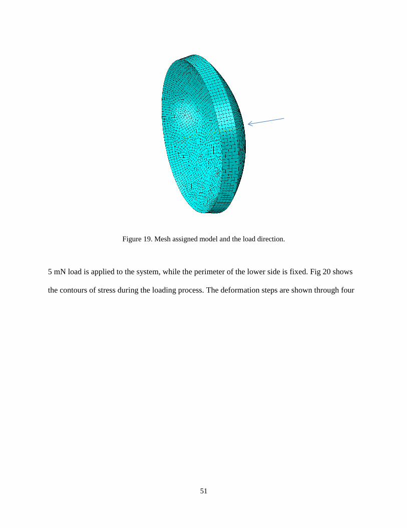
6.2.1. Case I: Point Load
In this scenario, a point nodal force is applied to the model. Material behavior is hyperelastic and
the values are implemented according to the results of the CG simulation. Fig. 19 shows the
initial model after meshing. Quad meshes are assigned with the total number of 6582 elements.
51
Figure 19. Mesh assigned model and the load direction.
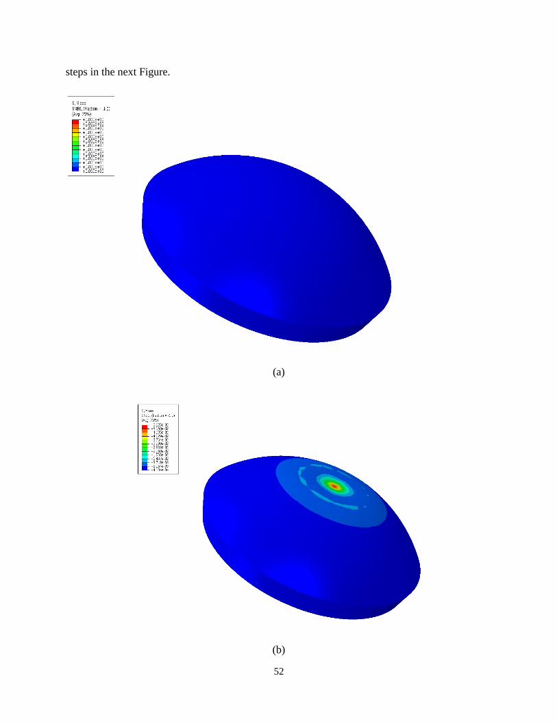
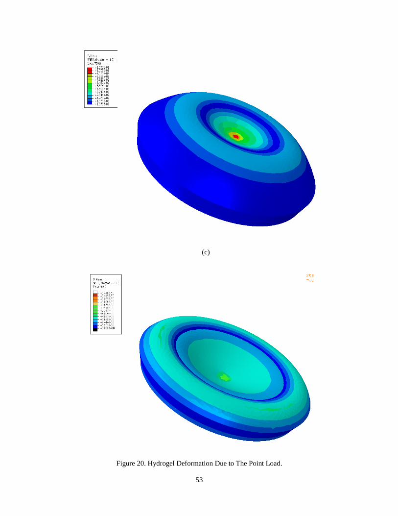
5 mN load is applied to the system, while the perimeter of the lower side is fixed. Fig 20 shows
the contours of stress during the loading process. The deformation steps are shown through four
52
steps in the next Figure.
(a)
(b)
53
(c)
Figure 20. Hydrogel Deformation Due to The Point Load.
54
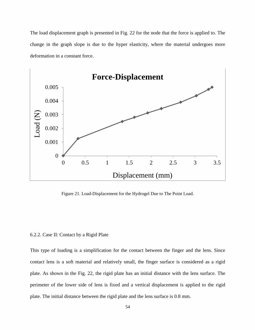
The load displacement graph is presented in Fig. 22 for the node that the force is applied to. The
change in the graph slope is due to the hyper elasticity, where the material undergoes more
deformation in a constant force.
Figure 21. Load-Displacement for the Hydrogel Due to The Point Load.
6.2.2. Case II: Contact by a Rigid Plate
This type of loading is a simplification for the contact between the finger and the lens. Since
contact lens is a soft material and relatively small, the finger surface is considered as a rigid
plate. As shown in the Fig. 22, the rigid plate has an initial distance with the lens surface. The
perimeter of the lower side of lens is fixed and a vertical displacement is applied to the rigid
plate. The initial distance between the rigid plate and the lens surface is 0.8 mm.
0
0.001
0.002
0.003
0.004
0.005
0 0.5 1 1.5 2 2.5 3 3.5
Load
(N
)
Displacement (mm)
Force-Displacement
55
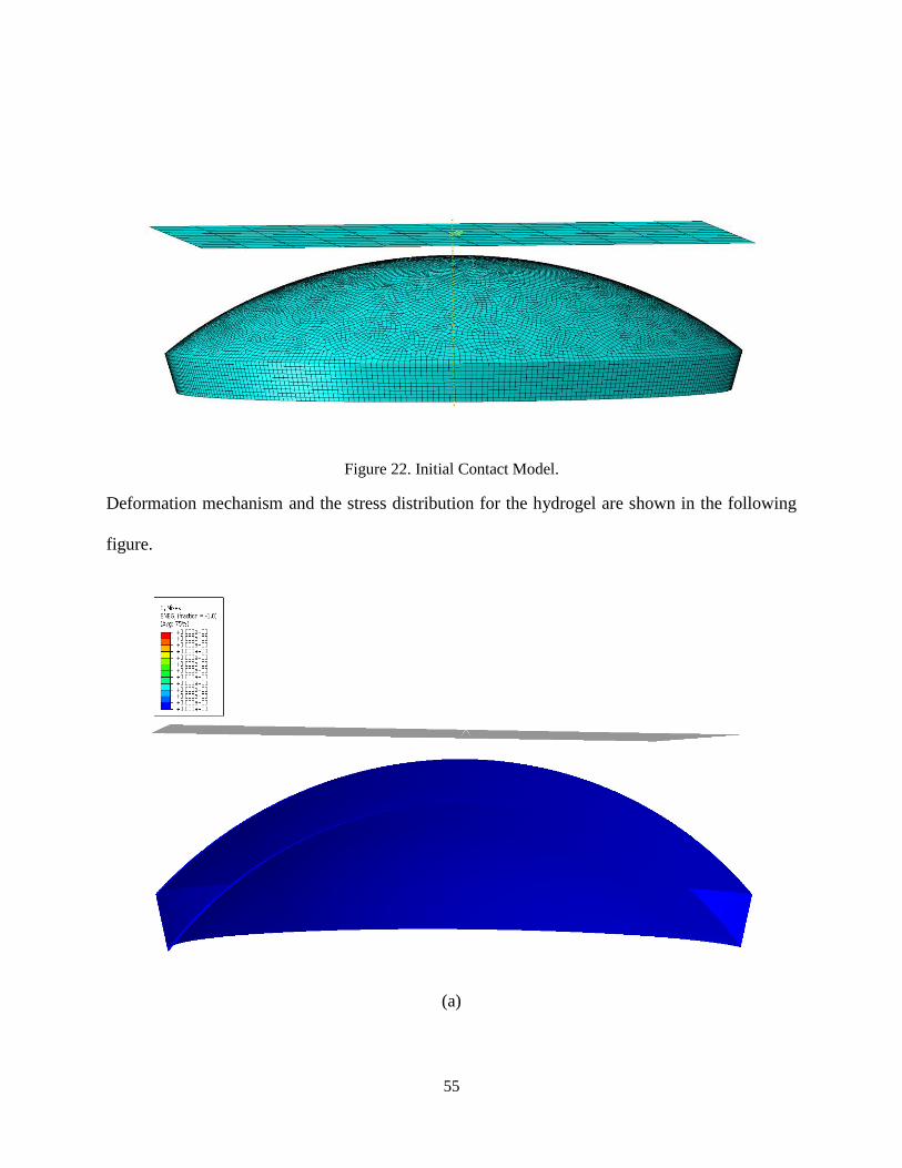
Figure 22. Initial Contact Model.
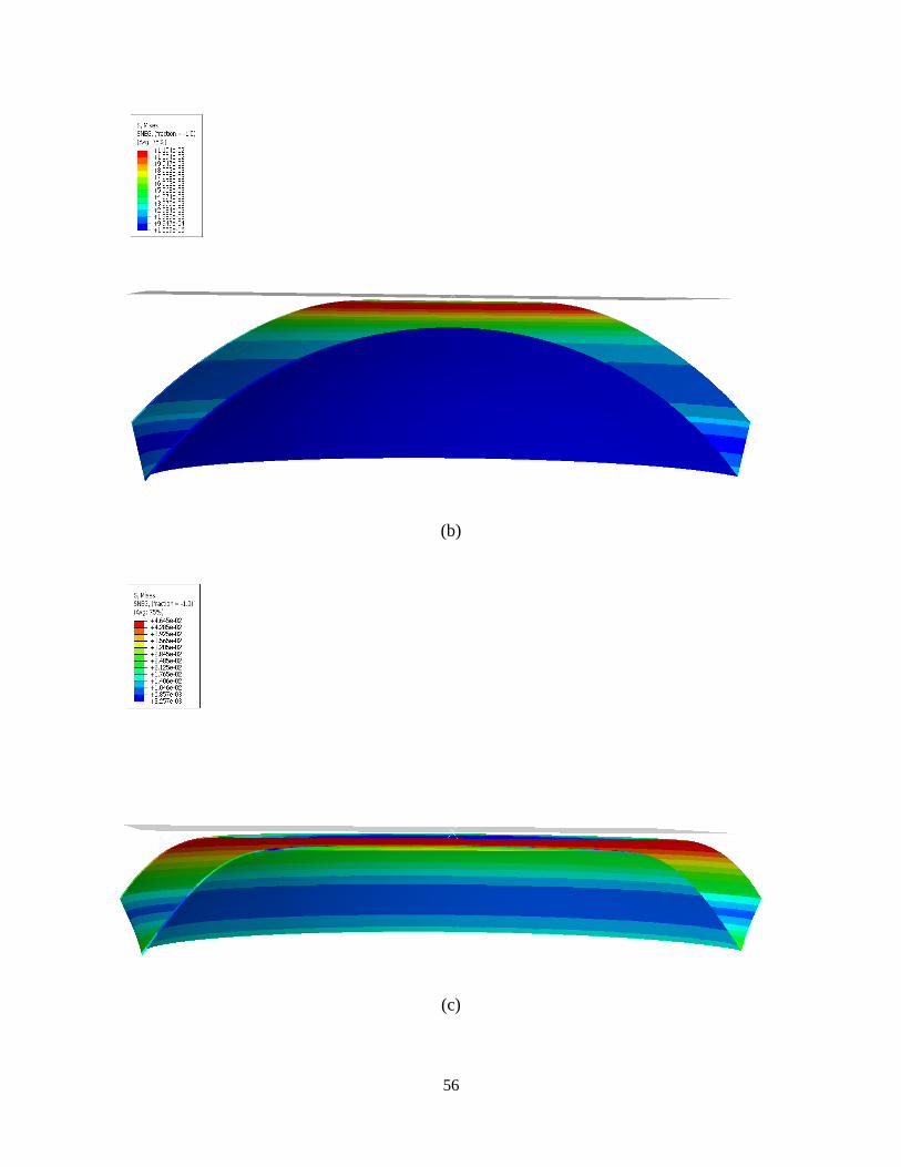
Deformation mechanism and the stress distribution for the hydrogel are shown in the following
figure.
(a)
56
(b)
(c)
57
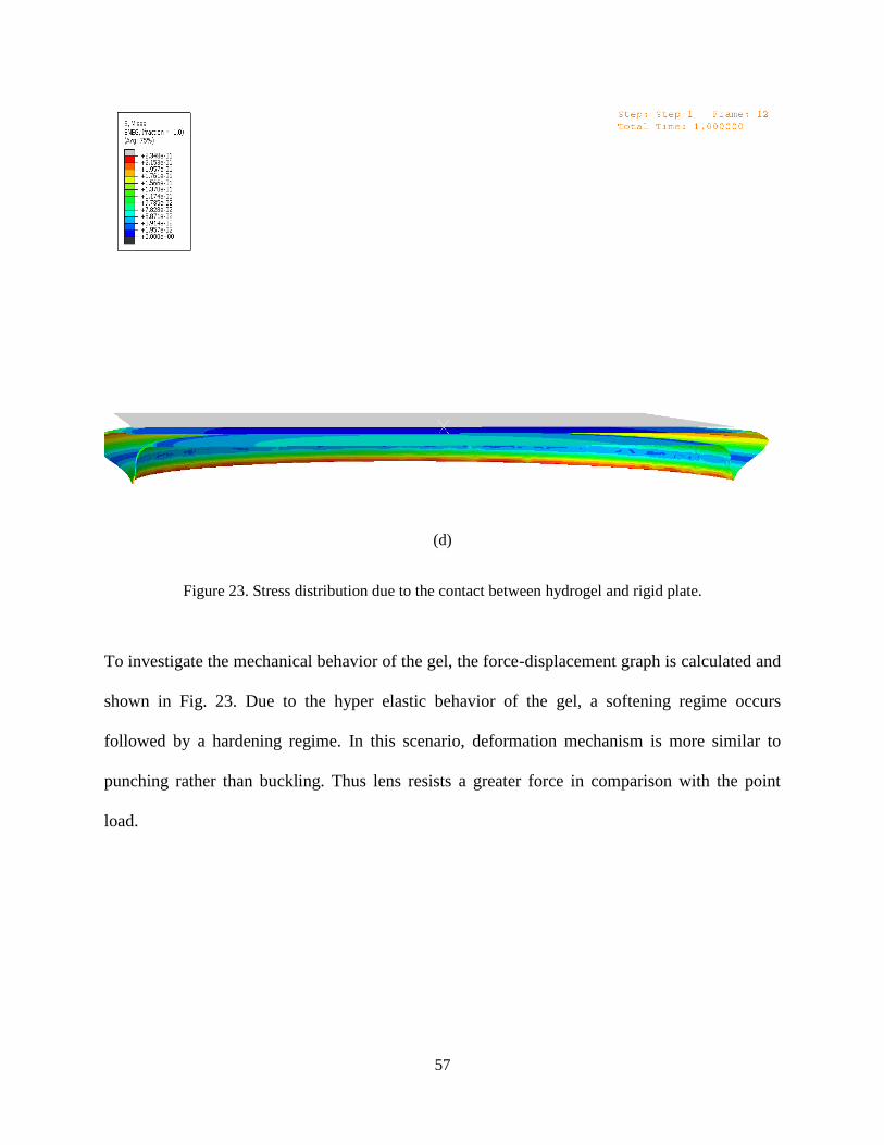
(d)
Figure 23. Stress distribution due to the contact between hydrogel and rigid plate.
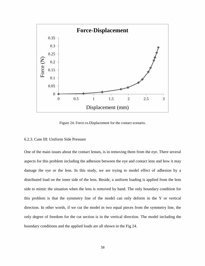
To investigate the mechanical behavior of the gel, the force-displacement graph is calculated and
shown in Fig. 23. Due to the hyper elastic behavior of the gel, a softening regime occurs
followed by a hardening regime. In this scenario, deformation mechanism is more similar to
punching rather than buckling. Thus lens resists a greater force in comparison with the point
load.
58
Figure 24. Force.vs.Displacement for the contact scenario.
6.2.3. Case III: Uniform Side Pressure
One of the main issues about the contact lenses, is in removing them from the eye. There several
aspects for this problem including the adhesion between the eye and contact lens and how it may
damage the eye or the lens. In this study, we are trying to model effect of adhesion by a
distributed load on the inner side of the lens. Beside, a uniform loading is applied from the lens
side to mimic the situation when the lens is removed by hand. The only boundary condition for
this problem is that the symmetry line of the model can only deform in the Y or vertical
direction. In other words, if we cut the model in two equal pieces from the symmetry line, the
only degree of freedom for the cut section is in the vertical direction. The model including the
boundary conditions and the applied loads are all shown in the Fig 24.
0
0.05
0.1
0.15
0.2
0.25
0.3
0.35
0 0.5 1 1.5 2 2.5 3
Fo
rce
(N)
Displacement (mm)
Force-Displacement
59
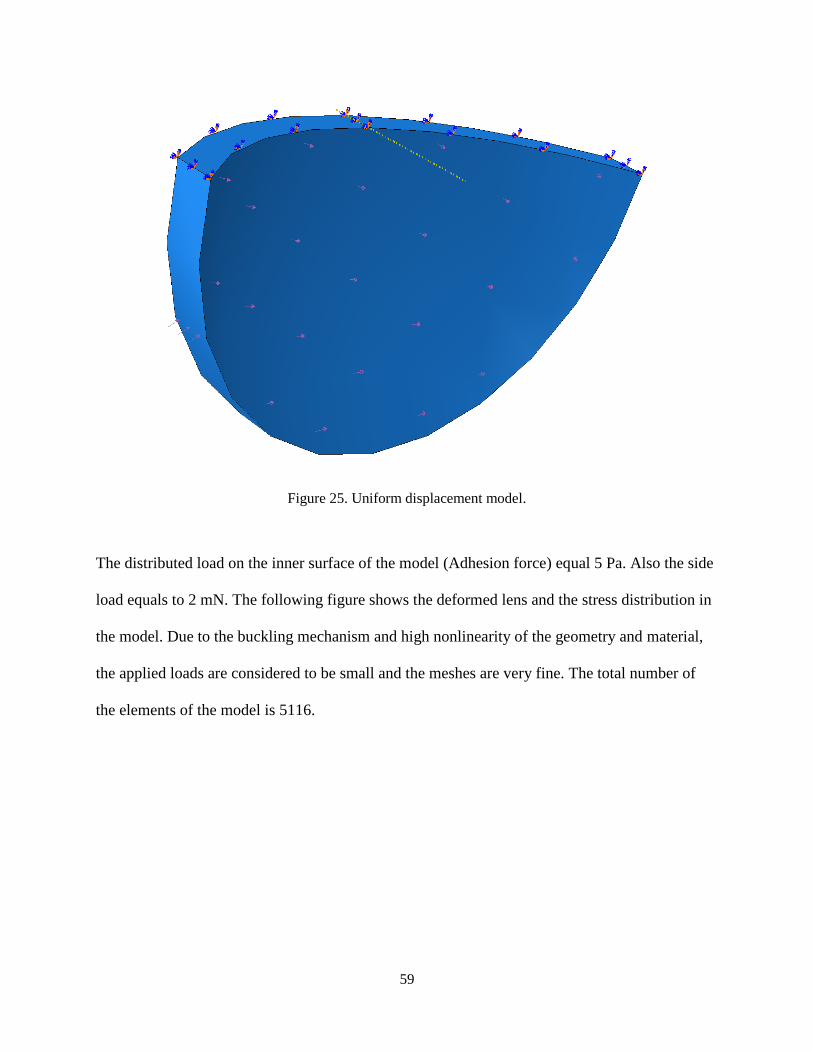
Figure 25. Uniform displacement model.
The distributed load on the inner surface of the model (Adhesion force) equal 5 Pa. Also the side
load equals to 2 mN. The following figure shows the deformed lens and the stress distribution in
the model. Due to the buckling mechanism and high nonlinearity of the geometry and material,
the applied loads are considered to be small and the meshes are very fine. The total number of
the elements of the model is 5116.
60
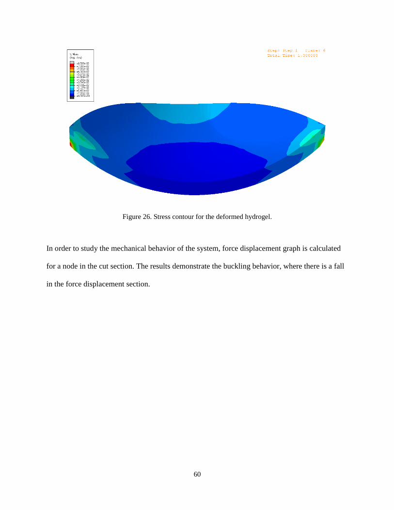
Figure 26. Stress contour for the deformed hydrogel.
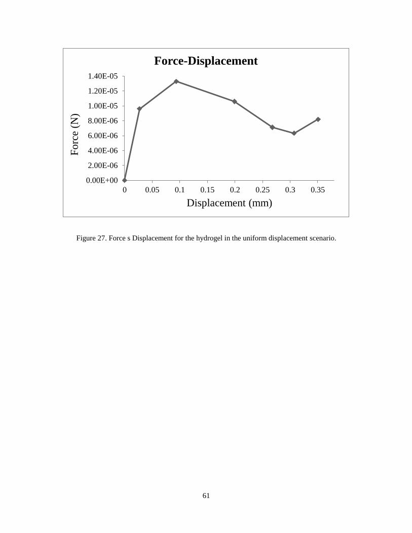
In order to study the mechanical behavior of the system, force displacement graph is calculated
for a node in the cut section. The results demonstrate the buckling behavior, where there is a fall
in the force displacement section.
61
Figure 27. Force s Displacement for the hydrogel in the uniform displacement scenario.
0.00E+00
2.00E-06
4.00E-06
6.00E-06
8.00E-06
1.00E-05
1.20E-05
1.40E-05
0 0.05 0.1 0.15 0.2 0.25 0.3 0.35
Fo
rce
(N)
Displacement (mm)
Force-Displacement
62
7. Summary
In this research, crosslinked hydrogels are studied through different scales. Molecular dynamics
simulations are performed to study the equilibrium structure and the effect of water on the elastic
properties of hydrogels. Analysis of structure through radial distribution functions shows that the
crosslink zones are the more hydrophilic parts of hydrogel. Also, the diffusion coefficients are
quantified for different water percentages, before and after the crosslinking. The elastic
properties are calculated. Since water molecules act as lubricators, an increase in water content
results in a decrease in Young Modulus. Coarse-Grained simulations are employed to study the
mechanical properties. A coarse-grained model is developed for the hydrogel using MARTINI
force-field. Shear simulation are performed for different water contents and the stress strain
curves are reported. The results show that the coarse-grained model captures the mechanical
properties more accurately and it has a good agreement with the experiment. Moreover, the
results show that the 40% water content is a crucial point and greater amounts of water leads to a
decrease in mechanical properties. Finally, continuum model of contact lens is studied under
three different loading scenarios of: point load, contact and uniform side pressure.
63
8. Recommendations and Future Work
There are several recommendations to continue the current research, among which is:
1. In this study effect of water on the mechanical properties are studied using atomistic
simulations. This research could be expanded to investigate the effect of temperature on the
elastic properties.
2. Coarse-Grained simulations are performed using the existing parameters of MARTINI
forcefield for polymers. DFT simulations could provide more accurate model of the hydrogels
and the parameters for the non-bonded interactions could be modified.
3. Tough hydrogels will be the ultimate solution for the cartilage replacement, as one the biggest
issues in biomedical engineering. In order to enhance the mechanical properties of hydrogels,
reinforcements could be applied. Studying adhesion mechanisms between the fibers and the
hydrogel using atomistic simulations will help to improve the toughening mechanisms.
4. Employing bottom-up approaches for designing hydrogels can’t be done, unless multi-scale
models are developed. In an up scaling paradigm, micro structure of the hydrogels will be
manipulated to reach to desired macro scale properties.
64
References
Allen, M. P, Tildesley, D. J, “Computer Simulation of Liquids”, New York: Oxford University
Press, 1987.
Brooks, B. R., Bruccoleri, R. E., Olafson, B. D., States, D. J., Swaminathan, S. and Karplus, M.
“Charmm: a Program for Macromolecular Energy, Minimization, and Dynamics Calculations,”
Journal of Computational Chemistry, 4:187-217, 1983.
Büyüköztürk, O., Buehler, M. J., Lau, D, Tuakta, C. “Structural Solution Using Molecular
Dynamics: Fundamentals and a Case study of Epoxy-Silica Interface” International Journal of
Solids and Structures. 48:2131–2140, 2011.
Calvert P. “Hydrogels for soft machines”. Adv Mater, 743–56, 2009.
Chiessi, E, Cavalieri. F, Paradossi, G, “Water and Polymer Dynamics in Chemically Cross-
Linked Hydrogels of Poly(vinyl alchohol): A Molecular Dynamics Simulation Study”, J. Phys.
Chem. B. 111:2820-2827, 2007.
P. Dauber-Osguthorpe, V.A. Roberts, D.J. Osguthorpe, J. Wolff, M. Genest, A.T. Hagler.
“Structure and energetics of ligand binding to proteins: E. coli dihydrofolate reductase-
trimethoprim, a drug-receptor system”, Proteins: Structure, Function and Genetics, 4:31–47,
1988.
Dumitriu, S. Dekker. M, “Polymeric Biomaterials,” New York, 2002.
Frenkel, D. and Smith, B. “Understanding molecular simulation “, Academic Press, San Diego,
2001.
65
Friends, G. D., Kunzler, J. F. and Ozark, R. M. “Recent Advances in the Design of Polymers for
Contact-Lenses,” Macromolecular Symposia, 98:619-631, 1995.
Garcia, F. G, Leyva, M. E, Alencar de Queiroz, A. A., Simoes, A. Z., “Durability of Adhesives
Based on Different Epoxy/Aliphatic Amine Networks”, International Journal of Adhesion and
Adhesives, 31:177, 2011.
Gautieri, A, Russo, A, Vesentini, S, Redaelli, A, Buhler, M. J, “Coarse-Grained Model of
Collagen Molecules Using an Extended MARTINI Force Field”, Journal of Chemical Theory
and Computations, 6:1210-1218, 2010.
Grujicic, M, Sun, Y. P, Koudela, K. L, “The effect of Covalent Functionalization of Carbon
Nanotube Reinforcements on The Atomic-Level Mechanical Properties of Poly-Vinyl-Ester-
Epoxy”, Applied Surface Science, 253:3009, 2007.
Harland, R. S., Prud’Homme, R. K., Eds. “Polyelectrolyte Gels: Properties, Preparation and
Applications”. American Chemical Society. Washington, DC, 1992.
Hoffman, A. S, “Hydrogels for Biomedical Applications”, Advanced Drug Delivery Reviews;
64:18–23 (2012).
Jang, S. S., Goddard, W. A. and Kalani, M. Y. S. “Mechanical and transport properties of the
poly(ethylene oxide)-poly(acrylic acid) double network hydrogel from molecular dynamic
simulations,” Journal of Physical Chemistry B, vol. 111:1729-1737, 2007.
Jang, S. S., Goddard, W. A., Kalani, M. Y. S., Myung, D. and Frank, C. W. “Mechanical and
transport properties of the poly(ethylene oxide)- poly(acrylic acid) double network hydrogel
from molecular dynamic Simulations,” Journal of Physical Chemistry B, 111:14440, 2007.
66
Langer, R. and Peppas, N. A. “Advances in biomaterials, drug delivery, and bionanotechnology,”
AIChE Journal, 49:2990-3006, 2003.
Lee, K. Y. and Mooney, D. J. “Hydrogels for tissue engineering,” Chemical Reviews, 101:1869-
1879, 2001.
Lee, S. G, Brunello. G. F, Jang, S. S, Bucknall, D. G. “Molecular Dynamics Simulation Study of
P(VP-co-HEMA) Hydrogels: Effect of Water Content on Equilibrium Structures and Mechanical
Properties” Biomaterials, 30:6130–6141, 2009.
Lee, S. G. “Structure-property Relationship of Hydrogel: Molecular Dynamics Simulation
Approach” PhD Dissertation, Georgia Institute of Technology, 2011.
Lowman, A. M, Peppas, N. A, Mathiowitz, E. “Hydrogels” Encyclopedia of controlled drug
delivery. John Wiley & Sons, 397–406, 1999.
Lu, Z, Dunn, M. L, “van der Waals Adhesion of Graphene Membranes”, Journal of Applied
Physics, 107:044301, 2010.
Maple, J. R, Dinur, U, Hagler, A. T, “Derivation of force fields for molecular mechanics and
dynamics from ab initio energy surfaces”, Progress of National Academy of Sciences of the
United States of America, 85: 5350–5354, 1988.
Marrink, S. J, Risselada, H. J, Yefimov, S, Tieleman, D. P, de Vries, A. H, “The MARTINI
Force Field: Coarse Grained Model For Biomolecular Simulations”, Journal of Physical
Chemistry B, 111:7812-7824, 2007.
67
Mayo, S. L., Olafson, B. D. and Goddard, W. A. “Dreiding - a generic force-field for molecular
simulations,” Journal of Physical Chemistry, 94: 8897-8909, 1990.
Oldiges, C. and Tonsing, T. “Molecular dynamic simulation of structural, mobility effects
between dilute aqueous CH3CN solution and crosslinked PAA - Part 1. Structure,” Physical
Chemistry Chemical Physics, 4: 1628-1636, 2002.
Oldiges, C., Tonsing, T. and Wittler, K. “Molecular dynamics simulation of structural, mobility
effects between dilute aqueous CH3CN solution and crosslinked PAA - Part 2. Dynamics,”
Physical Chemistry Chemical Physics, 4: 5135-5141, 2002.
Oldiges, C., Wittler, K., Tonsing, T. and Alijah, A. “MD calculated structural properties of
clusters in liquid acetonitrile/water mixtures with various contents of acetonitrile,” Journal of
Physical Chemistry A, 106: 7147-7154, 2002.
Peppas, N. A., Huang, Y., Torres-Lugo, M., Ward, J. H. and Zhang, J. “Physicochemical,
foundations and structural design of hydrogels in medicine and biology,” Annual Review of
Biomedical Engineering, 2: 9-29, 2000.
Peppas, N. A. “Hydrogels and drug delivery,” Current Opinion in Colloid & Interface Science,
2: 531-537, 1997.
Peppas NA, Hilt JZ, Khademhosseini A, Langer R. “Hydrogels in biology and medicine: from
fundamentals to bionanotechnology”. Adv Mater , 1345-60, 2006.
Potter, D. E. “Computational Physics,” John Wiley & Sons, New York, 1973.
Rappe, A. K, Goddard, W. A, “Charge Equilibration For Molecular Dynamics Simulations”, The
Journal of Physical Chemistry, 95, 3358, 1991.
68
Salahshoor, H, Rahbar, N, “Nano-scale Fracture Toughness and Behavior of Graphene/Epoxy
Interface”, Journal of Applied Physics,112:023510-1-6, 2012.
Sun, H. “COMPASS: An ab initio force field optimized for condensed-phase applications
overview with details on alkane and benzene compounds”. Phys. Chem. B 102:7338, 1998.
Sun, H, Ren, P, Fried, J. R, “The COMPASS force field: Parameterization and Validation for
Phosphazens”, Computational and Theoretical Polymer Science, 8 (1/2) 229, 1998.
Swope, W. C., Andersen, H. C., Berens, P. H. and Wilson, K. R. “A computer-simulation
method for the calculation of equilibrium-constants for the formation of physical clusters of
molecules - application to small water clusters,” J Chem Phys, 76: 637-649, 1982.
Tamai, Y., Tanaka, H. and Nakanishi, K. “Molecular dynamics study of polymer-water
interaction in hydrogels .2. Hydrogen-bond dynamics,” Macromolecules, 29: 6761-6769, 1996.
Tamai, Y. and Tanaka, H. “Effects of polymer chains on structure and dynamics of supercooled
water in poly(vinyl alcohol),” Physical Review E, 59: 5647-5654, 1999.
Tamai, Y. and Tanaka, H. “Structure and dynamics of poly(vinyl alcohol) hydrogel,” Molecular
Simulation, 21: 283-301, 1999.
Theodorou, D. N, Suter, U. W, “Detailed Molecular Structure of a Vinyl Polymer Glass”,
Macromolecules. 18, 1467, 1985.
Verlet, L. “Computer Experiments on Classical Fluids .I. Thermodynamical Properties of
Lennard-Jones Molecules,” Physical Review, 159: 98, 1967.
Wainwright SA, Biggs WD, Currey JD, Gosline JM. Mechanical design in organism. Princeton,
NY: Princeton University Press; 1986.
69
Walter, J, Ermatchkov, V, Vrabec, J, Hasse, H., “Molecular Dynamics and Experimental Study
of Conformation Change of Poly (N-isopropylacylamide) Hydrogels in Water” Fluid Phase
Equilibria. 296:164–172, 2010.
Weiner, S. J., Kollman, P. A., Case, D. A., Singh, U. C., Ghio, C., Alagona, G., Profeta, S. and
Weiner, P. “A New Force-Field for Molecular Mechanical Simulation of Nucleic-Acids and
Proteins,” Journal of the American Chemical Society, 106: 765-784, 1984.
Weiner, S. J., Kollman, P. A., Nguyen, D. T. and Case, D. A. “An All Atom Force-Field for
Simulations of Proteins and Nucleic-Acids,” Journal of Computational Chemistry, 7:230-252,
1986.
Wichterle, O. and Lim, D. “Hydrophilic gels for biological use”, Nature, 185: 117-118, 1960.
Wu, Y, Joseph, S, Aluru, N. R, “Effect of Cross-Linking on The Diffusion of Water, Ions, and
Small Molecules in Hydrogels” J. Phys. Chem. B. 113:3512–3520, 2009.
Wu, C, Xu, W, “Atomistic Molecular Modeling of Crosslinked Epoxy Resin”, Polymer,
47:6004-6009, 2006.