1

Paper presented at the Population Association of America 2011 Annual Meeting - Washington, DC. Session 125: Formal Demography I: Mathematical Models and Methods (Friday 1 April 2011, 12:30 PM - 2:20 PM)

Latest revision 6 April 2011

Modifying the Lee-Carter method to project mortality changes up to 2100 Nan Li and Patrick Gerland1 United Nations Population Division. Department for Economic and Social Affairs, United Nations, New York, NY 10017, USA. In the last half century and in countries without mortality crises, the common pattern of mortality decline is that death rate declined faster at younger ages than at older ages. In the future and in low mortality countries, however, such a pattern is believed to change. More specifically, the decline of infant and child mortality is expected to decelerate, and the reduction of old-age mortality to accelerate. In terms of the Lee-Carter method (1992), this change would require a rotation on the age pattern of mortality-decline rates. In projections of 50 years or so, dealing with the rotation was not found necessary. When the horizon extends to a century, however, the effects of this rotation remained largely unknown. In this paper, we investigate the necessity of modifying the Lee-Carter method to deal with this rotation, and provide an acceptable solution to extend the horizon of projection to year 2100. The background

In 1992, Lee and Carter published a method to forecast mortality change, which simplifies the change of a vector of age-specific death rates to the change of a scalar, and hence has been applied to many countries. Let the death rate for age x at time t be m(x,t), for t =0, 1, 2, …, T, and let the over-time average of log[m(x,t)] be a(x). The Lee-Carter method first uses the singular-value decomposition (SVD) on {log[m(x,t)]-a(x)} to obtain

),()()()()],(log[ txtkxbxatxm ε++= . (1) Equation (1) transfers the task of forecasting a vector log[m(x,t)] into forecasting a scalar k(t), with small errors ),( txε . The k(t) is then described by a standard time-series model, which further produces forecast of m(x,t) according to (1). In most applications, it has been found that a random walk with drift works well for k(t):

0))()((),1,0(~)(,)()1()( =++−= teseENtetedtktk σ . (2)

To utilise the Bayesian probabilistic projections on life expectancy (Chunn et al., 2010), we modified the Lee-Carter method by adjusting the k(t) to fit the project life

1 The views expressed in this paper are those of the authors and do not necessarily reflect those of the United Nations. Its contents has not been formally edited and cleared by the United Nations.

2

expectancy. In this paper, we rotate the age pattern of mortality-decline rates, which is the b(x) in (1), to make the projection more plausible in the long run. According to (1) and (2), the mean of mortality-decline rate at age x,

)],(/)1,([ txmtxmLog +− , is projected as )()()]1()([ xbdxbtktkmean ⋅−=−−− , which is also the average mortality-decline rate observed from the recent history. Standing on this objective basis, the Lee-Carter method could always provide reasonable projections of 50 years or so, for countries with smooth mortality declines in the recent history.

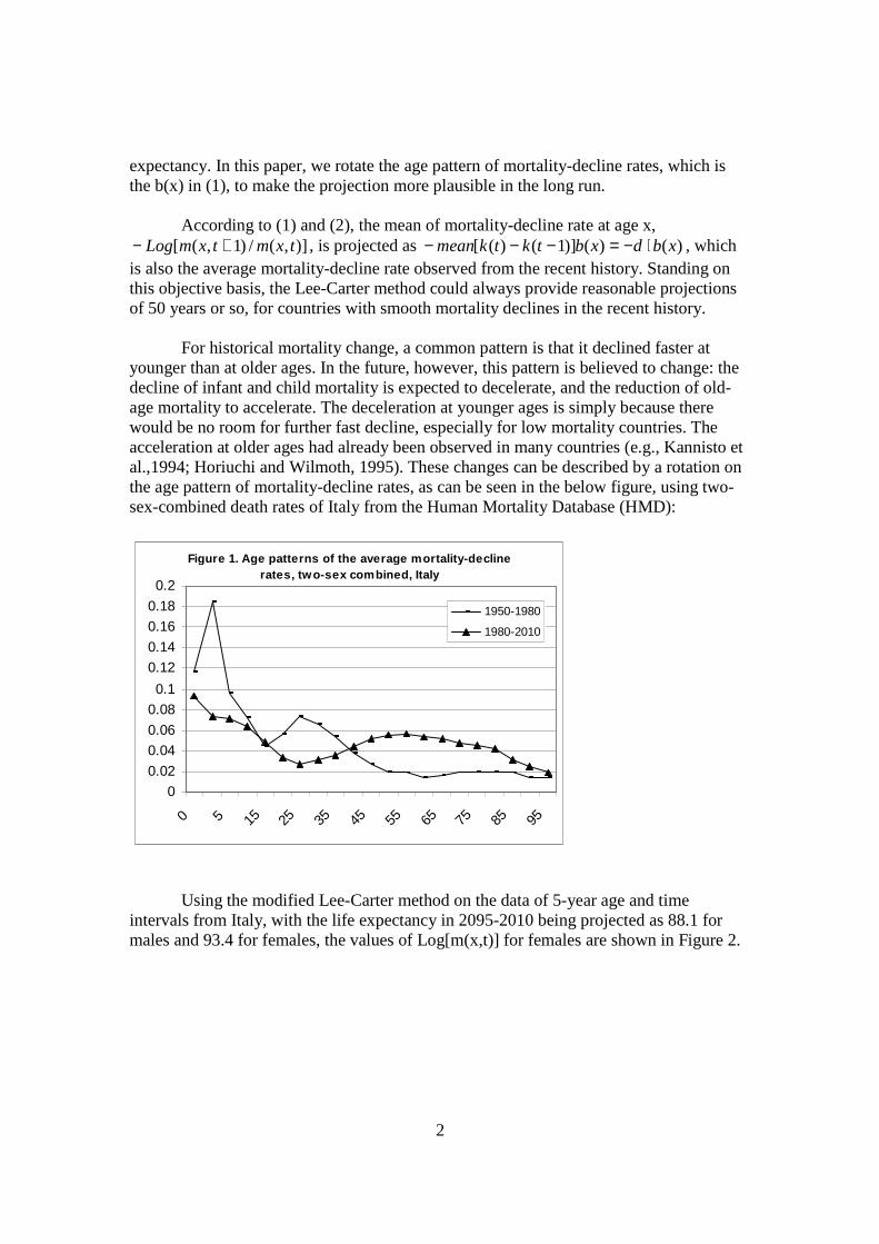
For historical mortality change, a common pattern is that it declined faster at younger than at older ages. In the future, however, this pattern is believed to change: the decline of infant and child mortality is expected to decelerate, and the reduction of old-age mortality to accelerate. The deceleration at younger ages is simply because there would be no room for further fast decline, especially for low mortality countries. The acceleration at older ages had already been observed in many countries (e.g., Kannisto et al.,1994; Horiuchi and Wilmoth, 1995). These changes can be described by a rotation on the age pattern of mortality-decline rates, as can be seen in the below figure, using two-sex-combined death rates of Italy from the Human Mortality Database (HMD):

Figure 1. Age patterns of the average mortality-decline rates, two-sex combined, Italy

0

0.02

0.04

0.06

0.08

0.1

0.12

0.14

0.16

0.18

0.2

0 5 15

25

35

45

55

65

75

85

95

1950-1980

1980-2010

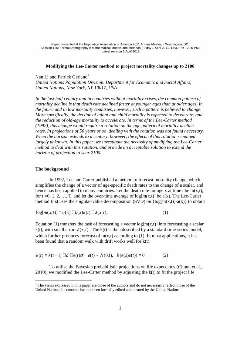
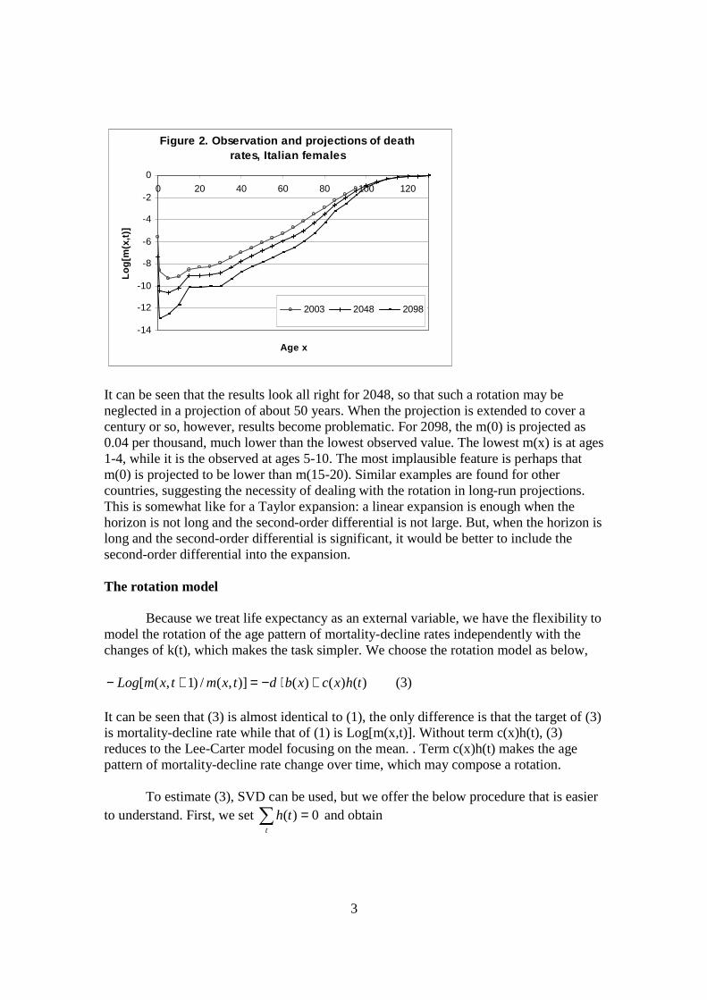
Using the modified Lee-Carter method on the data of 5-year age and time intervals from Italy, with the life expectancy in 2095-2010 being projected as 88.1 for males and 93.4 for females, the values of Log[m(x,t)] for females are shown in Figure 2.

3

Figure 2. Observation and projections of death rates, Italian females

-14

-12

-10

-8

-6

-4

-2

0

0 20 40 60 80 100 120

Age x

Lo

g[m

(x,t

)]

2003 2048 2098

It can be seen that the results look all right for 2048, so that such a rotation may be neglected in a projection of about 50 years. When the projection is extended to cover a century or so, however, results become problematic. For 2098, the m(0) is projected as 0.04 per thousand, much lower than the lowest observed value. The lowest m(x) is at ages 1-4, while it is the observed at ages 5-10. The most implausible feature is perhaps that m(0) is projected to be lower than m(15-20). Similar examples are found for other countries, suggesting the necessity of dealing with the rotation in long-run projections. This is somewhat like for a Taylor expansion: a linear expansion is enough when the horizon is not long and the second-order differential is not large. But, when the horizon is long and the second-order differential is significant, it would be better to include the second-order differential into the expansion. The rotation model

Because we treat life expectancy as an external variable, we have the flexibility to

model the rotation of the age pattern of mortality-decline rates independently with the changes of k(t), which makes the task simpler. We choose the rotation model as below,

)()()()],(/)1,([ thxcxbdtxmtxmLog +⋅−=+− (3) It can be seen that (3) is almost identical to (1), the only difference is that the target of (3) is mortality-decline rate while that of (1) is Log[m(x,t)]. Without term c(x)h(t), (3) reduces to the Lee-Carter model focusing on the mean. . Term c(x)h(t) makes the age pattern of mortality-decline rate change over time, which may compose a rotation. To estimate (3), SVD can be used, but we offer the below procedure that is easier to understand. First, we set 0)( =∑

t

th and obtain

4

T

txmtxmLogxbd

T

t∑

−

=

+=⋅

1

0

)],(/)1,([)( . (4)

Setting∑ = 1)(xb , we can separate d and b(x). Second, by setting ∑ −= 1)(xc , we

have

dtxmtxmLogthx

−+=∑ )],(/)1,([)( . (5)

Finally, c(x) is obtained using ordinary least square:

∑

∑ +=

t

t

th

txmtxmLogthxc

2)(

)],(/)1,([)()( . (6)

Applications to individual countries

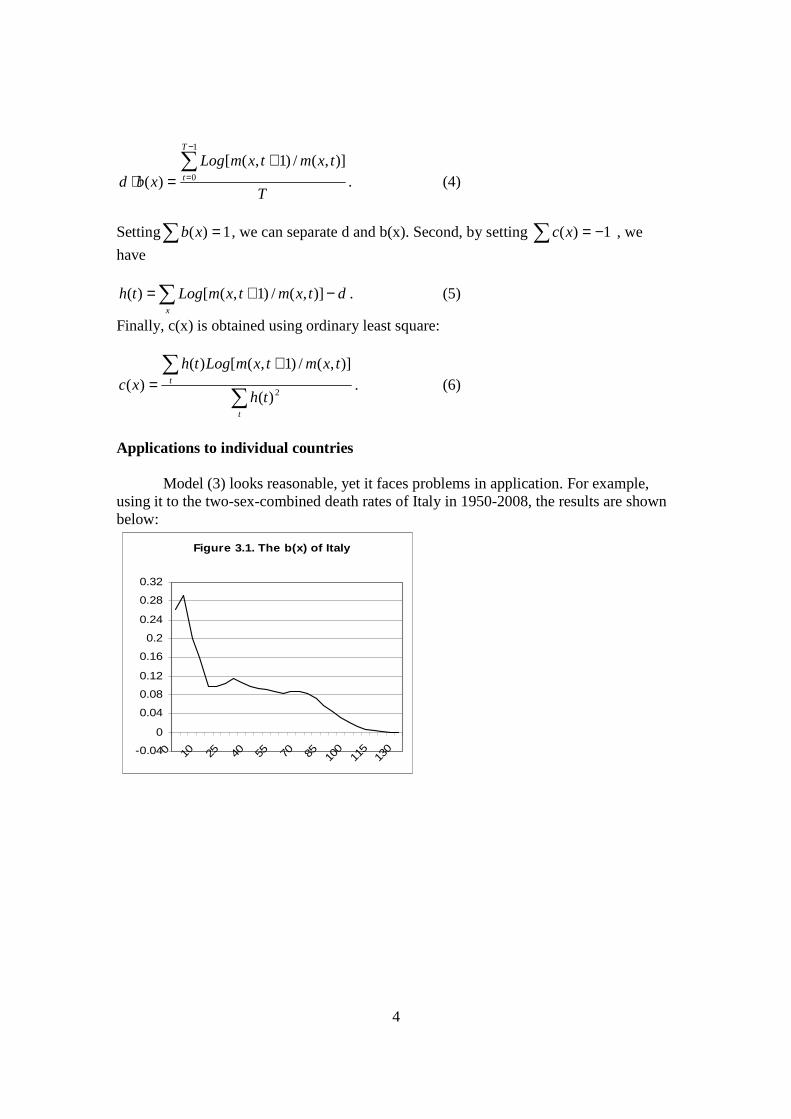
Model (3) looks reasonable, yet it faces problems in application. For example,

using it to the two-sex-combined death rates of Italy in 1950-2008, the results are shown below:

Figure 3.1. The b(x) of Italy

-0.04

0

0.04

0.08

0.12

0.16

0.2

0.24

0.28

0.32

0 10 25 40 55 70 85 100

115

130

5

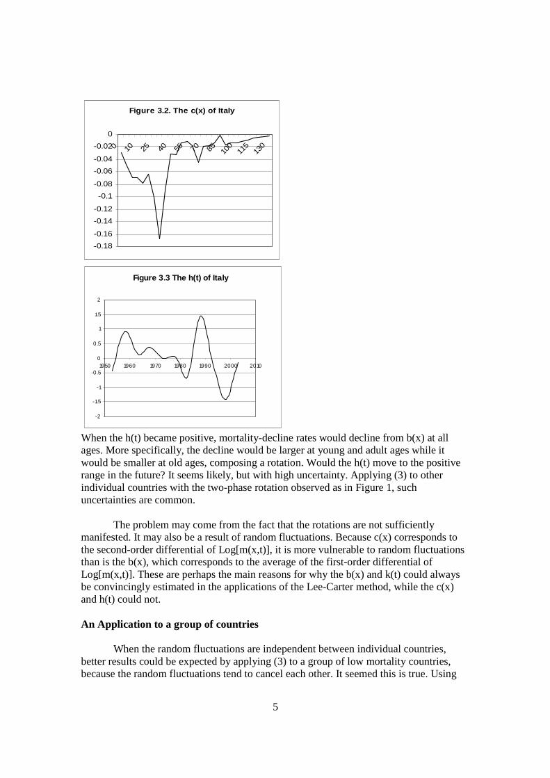
Figure 3.2. The c(x) of Italy

-0.18

-0.16

-0.14

-0.12

-0.1

-0.08

-0.06

-0.04

-0.02

0

0 10 25 40 55 70 85 100

115

130

Figure 3.3 The h(t) of Italy

-2

-1.5

-1

-0.5

0

0.5

1

1.5

2

1950 1960 1970 1980 1990 2000 2010

When the h(t) became positive, mortality-decline rates would decline from b(x) at all ages. More specifically, the decline would be larger at young and adult ages while it would be smaller at old ages, composing a rotation. Would the h(t) move to the positive range in the future? It seems likely, but with high uncertainty. Applying (3) to other individual countries with the two-phase rotation observed as in Figure 1, such uncertainties are common.

The problem may come from the fact that the rotations are not sufficiently manifested. It may also be a result of random fluctuations. Because c(x) corresponds to the second-order differential of Log[m(x,t)], it is more vulnerable to random fluctuations than is the b(x), which corresponds to the average of the first-order differential of Log[m(x,t)]. These are perhaps the main reasons for why the b(x) and k(t) could always be convincingly estimated in the applications of the Lee-Carter method, while the c(x) and h(t) could not. An Application to a group of countries When the random fluctuations are independent between individual countries, better results could be expected by applying (3) to a group of low mortality countries, because the random fluctuations tend to cancel each other. It seemed this is true. Using

6

the two-sex-combined death rates of the 11 countries2 weighted by population from HMD, results are shown in Figure 4:

Figure 4.1. The b(x) of 10 Europeran countries and New Zealand

0

0.04

0.08

0.12

0.16

0.2

0.24

0.28

0 10 25 40 55 70 85 100

115

130

Figure 4.2. The c(x) of 10 Europeran countries and New Zealand

-0.16

-0.14

-0.12

-0.1

-0.08

-0.06

-0.04

-0.02

0

0.02

0 10 25 40 55 70 85 100

115

130

2 Among all the 37 countries and areas listed in HMD, we found 23 have data for period 1950-2008 and experienced normal mortality changes. Among the 23 countries, we found 12 whose data showed the two-phase rotation as in Figure 1, of which Japan will be discussed separately for reasons to be seen. The left 11 countries are Belgium, Czech Republic, Finland, Ireland, Italy, New Zealand, Norway, Slovakia, Spain, Sweden, and Switzerland.

7

Figure 4.3 The h(t) of 10 Europeran countries and New Zealand

-2

-1.5

-1

-0.5

0

0.5

1

1.5

1950 1960 1970 1980 1990 2000 2010

Here the sharp of c(x) is similar to that of Italy, but the trend in h(t) is different: it looks to stay in the positive range more certain than the case of Italy. Moreover, 47% of the variance of using b(x) to describe mortality-decline rates is explained by c(x)h(t), comparing to 38% of Italy. Above results are obtained from two-sex combined data. Applying model (3) to the data of males or females of these countries, similar results are observed. A solution: the robust rotation How to model the h(t) for this group of countries is still a problem, because potential models are not unique. It will be more difficult, however, when requiring such a model be useful for individual countries.

Nonetheless, it is clear that if h(t) converges to values higher than 0.67, mortality-decline rates would become negative at adult ages. It is also clear that the rotation would be opposite, if h(t) drops to negative values. Given the upper and lower bounds, we may assume that after time T in the recent future, h(t) would converge to some value with declining fluctuations. Denoting by

)()()()( ThxcxbdxBr +⋅−= , (7)

we show the potential rotations in Figure 5, in which all Br(x) are rescaled to

1)( =∑x

xBr :

8

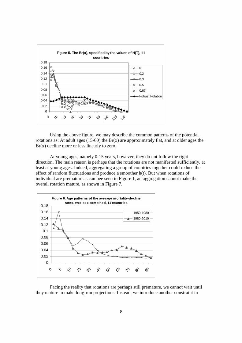
Figure 5. The Br(x), specified by the values of H(T), 11 countries

0

0.02

0.04

0.06

0.08

0.1

0.12

0.14

0.16

0.18

0 10 25 40 55 70 85 100

115

130

0

0.2

0.3

0.5

0.67

Robust Rotation

Using the above figure, we may describe the common patterns of the potential rotations as: At adult ages (15-60) the Br(x) are approximately flat, and at older ages the Br(x) decline more or less linearly to zero.

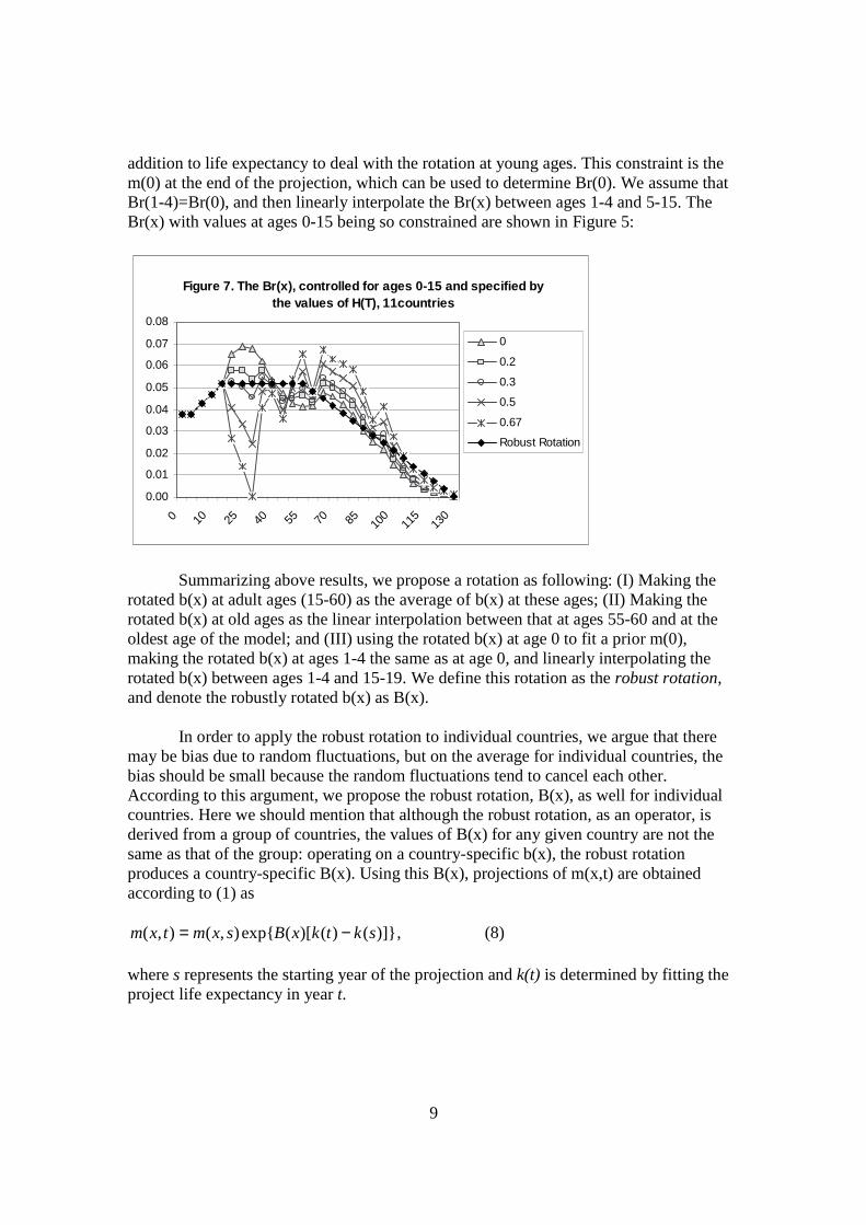
At young ages, namely 0-15 years, however, they do not follow the right direction. The main reason is perhaps that the rotations are not manifested sufficiently, at least at young ages. Indeed, aggregating a group of countries together could reduce the effect of random fluctuations and produce a smoother h(t). But when rotations of individual are premature as can bee seen in Figure 1, an aggregation cannot make the overall rotation mature, as shown in Figure 7.

Figure 6. Age patterns of the average mortality-decline rates, two-sex combined, 11 countries

0

0.02

0.04

0.06

0.08

0.1

0.12

0.14

0.16

0.18

0 5 15

25

35

45

55

65

75

85

95

1950-1980

1980-2010

Facing the reality that rotations are perhaps still premature, we cannot wait until

they mature to make long-run projections. Instead, we introduce another constraint in

9

addition to life expectancy to deal with the rotation at young ages. This constraint is the m(0) at the end of the projection, which can be used to determine Br(0). We assume that Br(1-4)=Br(0), and then linearly interpolate the Br(x) between ages 1-4 and 5-15. The Br(x) with values at ages 0-15 being so constrained are shown in Figure 5:

Figure 7. The Br(x), controlled for ages 0-15 and specified by the values of H(T), 11countries

0.00

0.01

0.02

0.03

0.04

0.05

0.06

0.07

0.08

0 10 25 40 55 70 85 100

115

130

0

0.2

0.3

0.5

0.67

Robust Rotation

Summarizing above results, we propose a rotation as following: (I) Making the

rotated b(x) at adult ages (15-60) as the average of b(x) at these ages; (II) Making the rotated b(x) at old ages as the linear interpolation between that at ages 55-60 and at the oldest age of the model; and (III) using the rotated b(x) at age 0 to fit a prior m(0), making the rotated b(x) at ages 1-4 the same as at age 0, and linearly interpolating the rotated b(x) between ages 1-4 and 15-19. We define this rotation as the robust rotation, and denote the robustly rotated b(x) as B(x).

In order to apply the robust rotation to individual countries, we argue that there may be bias due to random fluctuations, but on the average for individual countries, the bias should be small because the random fluctuations tend to cancel each other. According to this argument, we propose the robust rotation, B(x), as well for individual countries. Here we should mention that although the robust rotation, as an operator, is derived from a group of countries, the values of B(x) for any given country are not the same as that of the group: operating on a country-specific b(x), the robust rotation produces a country-specific B(x). Using this B(x), projections of m(x,t) are obtained according to (1) as

)]}()()[(exp{),(),( sktkxBsxmtxm −= , (8) where s represents the starting year of the projection and k(t) is determined by fitting the project life expectancy in year t.

10

The prior input How to input the prior m(0,2100)? Using the robust rotation, we first extended the Coale-Demeny model life tables to the life expectancy of 100 years (see annex), at which the m(0) are input as about 0.3 per thousand. Compared to the most recently observed lowest m(0) that is about 1 per thousand3, this input may not be entirely baseless. Given the project life expectancy for year 2100, we can find the corresponding m(0) from the West family of the Coale-Demeny model life tables, and use it as a reference for inputting m(0) in 2100. By doing so, we connect the prior input to observation, and also produce a consistent guideline for the input of individual countries. The case of Japan We mentioned above that the data of Japan also show a 2 two-phase rotation as in Figure 1, but we treated the case of Japan separately because its rotation is the most advanced among all other HMD countries. Applying (3) to the data of Japan, results are shown in Figure 8.

Figure 8.1. The b(x) of Japan

0

0.04

0.08

0.12

0.16

0.2

0.24

0.28

0.32

0.36

0 10 25 40 55 70 85 100

115

130

3 The lowest m(0) across the 101,232 annual life tables in the Human Mortality Database (as of 5 May 2010) covering 44 countries or areas from 1751 until 2008 was recorded in Iceland: 0.9 per thousand for female in 2007 and 1.3 per thousand for male in 2006 (Human Mortality Database, 2010).

11

Figure 8.2. The c(x) of Japan

-0.2

-0.15

-0.1

-0.05

0

0.05

0 10 25 40 55 70 85 100

115

130

Figure 8.3 The h(t) of Japan

-2

-1.5

-1

-0.5

0

0.5

1

1.5

2

1950 1960 1970 1980 1990 2000 2010

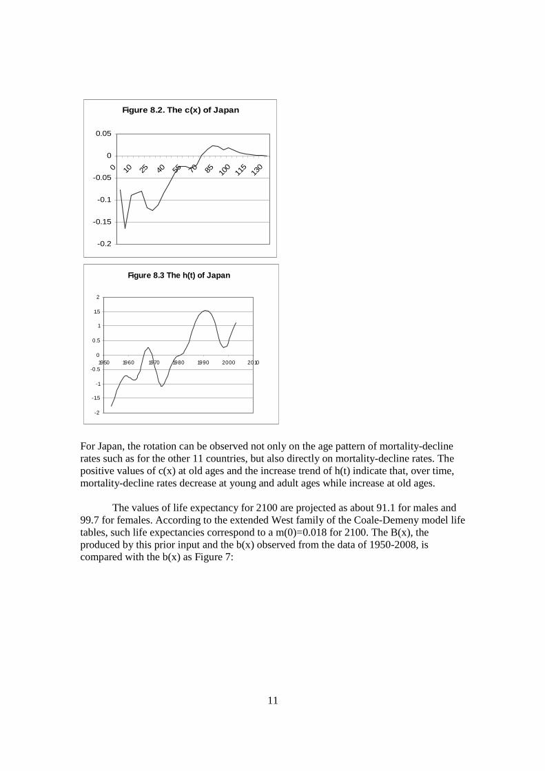
For Japan, the rotation can be observed not only on the age pattern of mortality-decline rates such as for the other 11 countries, but also directly on mortality-decline rates. The positive values of c(x) at old ages and the increase trend of h(t) indicate that, over time, mortality-decline rates decrease at young and adult ages while increase at old ages. The values of life expectancy for 2100 are projected as about 91.1 for males and 99.7 for females. According to the extended West family of the Coale-Demeny model life tables, such life expectancies correspond to a m(0)=0.018 for 2100. The B(x), the produced by this prior input and the b(x) observed from the data of 1950-2008, is compared with the b(x) as Figure 7:

12

Figure 9. The age patterns mortality-decline rates, Japan

0

0.01

0.02

0.03

0.04

0.05

0.06

0.07

0.08

0.09

0.1

0 10 25 40 55 70 85 100

115

130

The b(x) of 1950-2008

B(x)

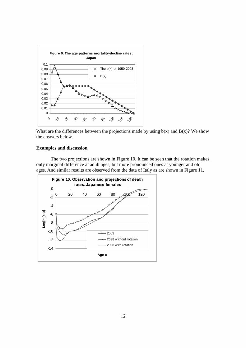
What are the differences between the projections made by using b(x) and B(x)? We show the answers below. Examples and discussion The two projections are shown in Figure 10. It can be seen that the rotation makes only marginal difference at adult ages, but more pronounced ones at younger and old ages. And similar results are observed from the data of Italy as are shown in Figure 11.

Figure 10. Observation and projections of death rates, Japanese females

-14

-12

-10

-8

-6

-4

-2

0

0 20 40 60 80 100 120

Age x

Lo

g[m

(x,t

)]

2003

2098 w ithout rotation

2098 w ith rotation

13

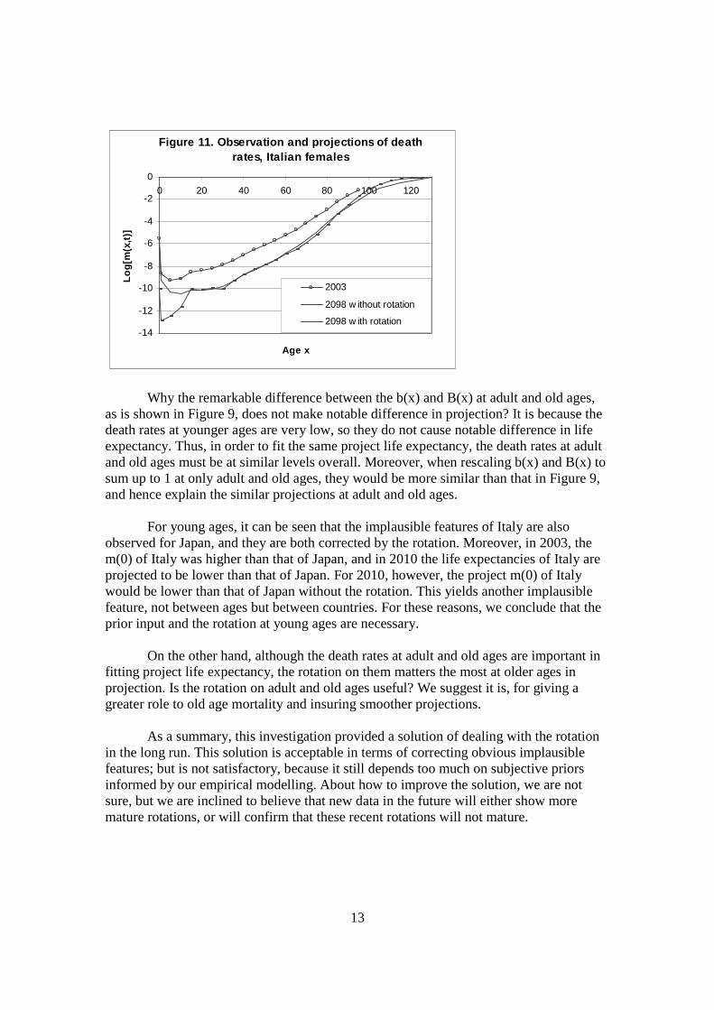
Figure 11. Observation and projections of death rates, Italian females

-14

-12

-10

-8

-6

-4

-2

0

0 20 40 60 80 100 120

Age x

Lo

g[m

(x,t

)]

2003

2098 w ithout rotation

2098 w ith rotation

Why the remarkable difference between the b(x) and B(x) at adult and old ages, as is shown in Figure 9, does not make notable difference in projection? It is because the death rates at younger ages are very low, so they do not cause notable difference in life expectancy. Thus, in order to fit the same project life expectancy, the death rates at adult and old ages must be at similar levels overall. Moreover, when rescaling b(x) and B(x) to sum up to 1 at only adult and old ages, they would be more similar than that in Figure 9, and hence explain the similar projections at adult and old ages.

For young ages, it can be seen that the implausible features of Italy are also observed for Japan, and they are both corrected by the rotation. Moreover, in 2003, the m(0) of Italy was higher than that of Japan, and in 2010 the life expectancies of Italy are projected to be lower than that of Japan. For 2010, however, the project m(0) of Italy would be lower than that of Japan without the rotation. This yields another implausible feature, not between ages but between countries. For these reasons, we conclude that the prior input and the rotation at young ages are necessary.

On the other hand, although the death rates at adult and old ages are important in

fitting project life expectancy, the rotation on them matters the most at older ages in projection. Is the rotation on adult and old ages useful? We suggest it is, for giving a greater role to old age mortality and insuring smoother projections. As a summary, this investigation provided a solution of dealing with the rotation in the long run. This solution is acceptable in terms of correcting obvious implausible features; but is not satisfactory, because it still depends too much on subjective priors informed by our empirical modelling. About how to improve the solution, we are not sure, but we are inclined to believe that new data in the future will either show more mature rotations, or will confirm that these recent rotations will not mature.

14

References Buettner, T. 2002. "Approaches and experiences in projecting mortality patterns for the oldest-old." North American Actuarial Journal 6(3):14-29. Chunn, J. L., Raftery, A. E., Gerland, P. 2010. Bayesian Probabilistic Projections of Mortality. Presented at the Annual Meeting of the Population Association of America. 15-17 April 2010, Dallas, TX. http://paa2010.princeton.edu/download.aspx?submissionId=101753 Coale, A. J. and P. Demeny. 1966. Regional Model Life Tables and Stable Populations. Princeton University Press. Coale, A. J. and G. Guo. 1989. Revised regional model life tables at very low levels of mortality." Population Index 55(4):613-643. Horiuchi, S. and J.R. Wilmoth. 1995. The Aging of Mortality Decline. Presented at the Annual Meeting of the Population Association of America, April 6, San Francisco. Human Mortality Database. University of California, Berkeley (USA), and Max Planck Institute for Demographic Research (Germany). Available at www.mortality.org or www.humanmortality.de (data downloaded on 5 May 2010). Kannisto, V., J. Lauristsen, A.R. Thatcher, and J.W. Vaupel. 1994. Reductions in Mortality at Advanced Ages: Several Decades of Evidence From 27 Countries. Population and Development Review 20:793-810. Lee, R. D. and L. Carter, 1992. Modeling and Forecasting the Time Series of U.S. Mortality. Journal of the American Statistical Association 87: 659—71. Li, N. and R. Lee, 2005. Coherent Mortality Forecasts for a Group of Populations - An Extension of the Lee-Carter Method. Demography, 42(3):575-594. United Nations. 1982. Model life tables for developing countries. Population Studies, 77. New York: United Nations. Wilmoth, J., V. Canudas-Romo, S. Zureick, M. Inoue, and C. Sawyer. 2009. "A Flexible Two-Dimensional Mortality Model for Use in Indirect Estimation." Presented at the Annual Meeting for the Population Association of America.

15

Annex: extension of the standard model life tables from 75 to 100 years of life expectancy at birth Background: two sets of standard model life table families (Coale-Demeny 1966 and 1989, and United Nations, 1982) are commonly used to derive a variety of mortality indicators and as underlying mortality patterns for estimation and projection by the United Nations and the demographic research community at large. But these two sets of model life tables - designed primarily to be used in developing countries or for historical populations – cover mortality patterns for life span only from age 20 to 75. A first extension of these model life tables was produced by Thomas Buettner in 1998 which extended the initials sets of model life tables from e(0)=75.0 up to 92.5 using both a limit life table as asymptotic pattern and the classic Lee-Carter approach to derive intermediate age patterns (Buettner, 2002). With the extension of the projection horizon for all countries up to 2100 as part of the 2010 revision of the UN World Population Prospects, it was necessary to allow life expectancy at birth to go beyond 92.5 years. In addition, additional in-depth analysis of the initial 1998 extension revealed substantial deviation for out-of-sample predictions compared to the Human Mortality Database experience at very low mortality levels (especially for Coale-Demeny models, see Figure 1 in Willmoth et al., 2009), and the need to improve a smoother transition between the existing set of model life tables up to age 75 and their extension. A new set extended model life tables were computed in Spring 2010 by staff of the Population Division (Gerland and Li) based on the modified Lee-Carter approach presented herein, and after extensive cross-validation against the Human Mortality Database (HMD) performed by Kirill Andreev, we imposed some constraints to insure some convergence toward the HMD mortality experience at high levels of e(0). The nine families of model life tables extended up to e(0)=100 were smoothly blended to the existing ones to insure smooth mortality surfaces by age and sex and e(0) levels. Synoptic of the analytical approach used:

1. This new series of model life tables is based on the original published set of mortality rates age and sex by Coale-Demeny (extended by Coale-Guo up to 75) and the United Nations (1982) from age 20 up to age 75 by 2.5 years increments.

2. For each sex and each of the nine model life table families, the initial set of mortality rates were refitted using first a classic Lee-Carter model developed by Nan Li which introduces the time dimension into the network of model life tables so that the corresponding k(t) appears linear between life expectancy at birth varying from 20 to 75.

3. The extension from age 75 to 100 years of life expectancy at birth was done using initially a non-divergent Lee-Carter model (Li and Lee, 2005) with linear k(t) and the age pattern a(x) at the highest level of life expectancy (i.e. 75) was used for projection up to age 100.

16

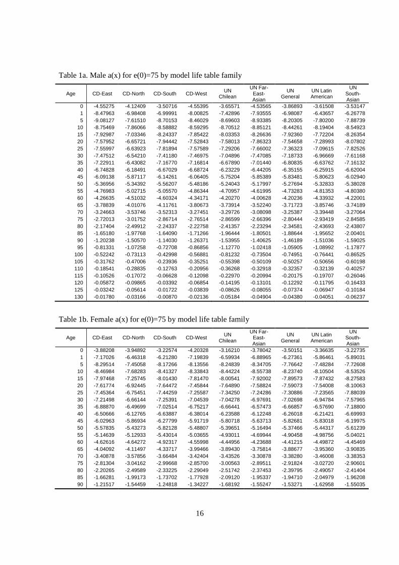
Table 1a. Male a(x) for e(0)=75 by model life table family

Age CD-East CD-North CD-South CD-West UN Chilean

UN Far-East-Asian

UN General

UN Latin American

UN South-Asian

0 -4.55275 -4.12409 -3.50716 -4.55395 -3.65571 -4.53565 -3.86893 -3.61508 -3.53147 1 -8.47963 -6.98408 -6.99991 -8.00825 -7.42896 -7.93555 -6.98087 -6.43657 -6.26778 5 -9.08127 -7.61510 -8.70153 -8.46029 -8.69603 -8.93385 -8.20305 -7.80200 -7.88739

10 -8.75469 -7.86066 -8.58882 -8.59295 -8.70512 -8.85121 -8.44261 -8.19404 -8.54923 15 -7.92987 -7.03346 -8.24337 -7.85422 -8.03353 -8.26636 -7.92360 -7.72204 -8.26354 20 -7.57952 -6.65721 -7.94442 -7.52843 -7.58013 -7.86323 -7.54658 -7.28993 -8.07802 25 -7.55997 -6.63923 -7.81894 -7.57589 -7.29206 -7.66002 -7.36323 -7.09615 -7.82526 30 -7.47512 -6.54210 -7.41180 -7.46975 -7.04896 -7.47085 -7.18733 -6.96669 -7.61168 35 -7.22911 -6.43082 -7.16770 -7.16814 -6.67890 -7.01440 -6.80835 -6.63762 -7.16132 40 -6.74828 -6.18491 -6.67029 -6.68724 -6.23229 -6.44205 -6.35155 -6.25915 -6.62004 45 -6.09138 -5.87117 -6.14261 -6.06405 -5.75204 -5.85389 -5.83481 -5.80623 -6.02940 50 -5.36956 -5.34392 -5.56207 -5.48186 -5.24043 -5.17997 -5.27694 -5.32833 -5.38028 55 -4.76983 -5.02715 -5.05570 -4.86344 -4.70957 -4.61995 -4.73283 -4.81353 -4.80380 60 -4.26635 -4.51032 -4.60324 -4.34171 -4.20270 -4.00628 -4.20236 -4.33932 -4.22001 65 -3.78839 -4.01076 -4.11761 -3.80673 -3.73914 -3.52240 -3.71723 -3.85746 -3.74189 70 -3.24663 -3.53746 -3.52313 -3.27451 -3.29726 -3.08098 -3.25387 -3.39448 -3.27064 75 -2.72013 -3.01752 -2.86714 -2.76514 -2.86599 -2.66396 -2.80444 -2.93419 -2.84585 80 -2.17404 -2.49912 -2.24337 -2.22758 -2.41357 -2.23294 -2.34581 -2.43693 -2.43807 85 -1.65180 -1.97768 -1.64090 -1.71266 -1.96444 -1.80501 -1.88644 -1.95652 -2.00401 90 -1.20238 -1.50570 -1.14030 -1.26371 -1.53955 -1.40625 -1.46189 -1.51036 -1.59025 95 -0.81331 -1.07258 -0.72708 -0.86856 -1.12770 -1.02418 -1.05905 -1.08992 -1.17877

100 -0.52242 -0.73113 -0.42998 -0.56881 -0.81232 -0.73504 -0.74951 -0.76441 -0.86525 105 -0.31762 -0.47006 -0.23936 -0.35251 -0.55398 -0.50109 -0.50257 -0.50656 -0.60198 110 -0.18541 -0.28835 -0.12763 -0.20956 -0.36268 -0.32918 -0.32357 -0.32139 -0.40257 115 -0.10526 -0.17072 -0.06628 -0.12098 -0.22970 -0.20994 -0.20175 -0.19707 -0.26046 120 -0.05872 -0.09865 -0.03392 -0.06854 -0.14195 -0.13101 -0.12292 -0.11795 -0.16433 125 -0.03242 -0.05614 -0.01722 -0.03839 -0.08626 -0.08055 -0.07374 -0.06947 -0.10184 130 -0.01780 -0.03166 -0.00870 -0.02136 -0.05184 -0.04904 -0.04380 -0.04051 -0.06237

Table 1b. Female a(x) for e(0)=75 by model life table family

Age CD-East CD-North CD-South CD-West UN Chilean

UN Far-East-Asian

UN General

UN Latin American

UN South-Asian

0 -3.88208 -3.94892 -3.22574 -4.20328 -3.16210 -3.78042 -3.50151 -3.36635 -3.22735 1 -7.17026 -6.46318 -6.21280 -7.19839 -6.59934 -6.88965 -6.27361 -5.86461 -5.89031 5 -8.29514 -7.45058 -8.17266 -8.13556 -8.24839 -8.34705 -7.76642 -7.48284 -7.72608

10 -8.46984 -7.68283 -8.41327 -8.33843 -8.44224 -8.55738 -8.23740 -8.10504 -8.53526 15 -7.97468 -7.25745 -8.01430 -7.81470 -8.00541 -7.92002 -7.89573 -7.87432 -8.27583 20 -7.61774 -6.92445 -7.64472 -7.45844 -7.64890 -7.58824 -7.59073 -7.54008 -8.10063 25 -7.45364 -6.75451 -7.44259 -7.25587 -7.34250 -7.24286 -7.30886 -7.23565 -7.88039 30 -7.21498 -6.66144 -7.25391 -7.04539 -7.04278 -6.97691 -7.02698 -6.94784 -7.57965 35 -6.88870 -6.49699 -7.02514 -6.75217 -6.66441 -6.57473 -6.66857 -6.57690 -7.18800 40 -6.50666 -6.12765 -6.63887 -6.38014 -6.23588 -6.12248 -6.26018 -6.21421 -6.69993 45 -6.02963 -5.86934 -6.27799 -5.91719 -5.80718 -5.63713 -5.82681 -5.83018 -6.19975 50 -5.57835 -5.43273 -5.82128 -5.48807 -5.39651 -5.16494 -5.37466 -5.44317 -5.61239 55 -5.14639 -5.12933 -5.43014 -5.03655 -4.93011 -4.69944 -4.90458 -4.98756 -5.04021 60 -4.62616 -4.64272 -4.92317 -4.55998 -4.44956 -4.23688 -4.41215 -4.49872 -4.45469 65 -4.04092 -4.11497 -4.33717 -3.99466 -3.89430 -3.75814 -3.88677 -3.95360 -3.90835 70 -3.40878 -3.57856 -3.66484 -3.42404 -3.43526 -3.30878 -3.38280 -3.46008 -3.38353 75 -2.81304 -3.04162 -2.99668 -2.85700 -3.00563 -2.89511 -2.91824 -3.02720 -2.90601 80 -2.20265 -2.49589 -2.33225 -2.29049 -2.51742 -2.37453 -2.39795 -2.49057 -2.41404 85 -1.66281 -1.99173 -1.73702 -1.77928 -2.09120 -1.95337 -1.94710 -2.04979 -1.96208 90 -1.21517 -1.54459 -1.24818 -1.34227 -1.68192 -1.55247 -1.53271 -1.62958 -1.55035

17

Age CD-East CD-North CD-South CD-West UN Chilean

UN Far-East-Asian

UN General

UN Latin American

UN South-Asian

95 -0.84749 -1.14355 -0.85293 -0.96799 -1.28581 -1.17587 -1.15070 -1.23335 -1.16787 100 -0.54458 -0.80208 -0.52819 -0.65301 -0.96393 -0.86924 -0.83366 -0.90864 -0.84924 105 -0.33504 -0.53674 -0.31172 -0.42159 -0.69015 -0.61459 -0.57752 -0.63877 -0.59083 110 -0.19789 -0.34377 -0.17586 -0.26118 -0.47573 -0.41890 -0.38480 -0.43169 -0.39539 115 -0.11361 -0.21263 -0.09628 -0.15690 -0.31724 -0.27678 -0.24827 -0.28212 -0.25618 120 -0.06405 -0.12823 -0.05176 -0.09230 -0.20604 -0.17851 -0.15633 -0.17964 -0.16194 125 -0.03572 -0.07605 -0.02754 -0.05357 -0.13122 -0.11313 -0.09676 -0.11227 -0.10061 130 -0.01980 -0.04462 -0.01457 -0.03084 -0.08244 -0.07084 -0.05922 -0.06928 -0.06178

Figure 13. a(x) by sex for e(0)=75 by model life table family

-10.00000

-9.00000

-8.00000

-7.00000

-6.00000

-5.00000

-4.00000

-3.00000

-2.00000

-1.00000

0.00000

0 20 40 60 80 100 120

Male CD-East

CD-North

CD-South

CD-West

UN Chilean

UN Far-East-Asian

UN General

UN Latin American

UN South-Asian

-9.00000

-8.00000

-7.00000

-6.00000

-5.00000

-4.00000

-3.00000

-2.00000

-1.00000

0.00000

0 20 40 60 80 100 120

Female CD-East

CD-North

CD-South

CD-West

UN Chilean

UN Far-East-Asian

UN General

UN Latin American

UN South-Asian

18

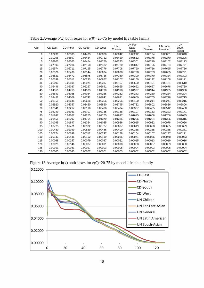
Table 2.Average b(x) both sexes for e(0)=20-75 by model life table family

Age CD-East CD-North CD-South CD-West UN Chilean

UN Far-East-Asian

UN General

UN Latin American

UN South-Asian

0 0.07239 0.06303 0.04473 0.06880 0.05042 0.05212 0.05124 0.05081 0.05048 1 0.10298 0.08897 0.08454 0.09712 0.08420 0.08512 0.08378 0.08270 0.08226 5 0.08803 0.08063 0.08454 0.07750 0.08233 0.08301 0.08219 0.08162 0.08173

10 0.07193 0.07016 0.07158 0.07482 0.07780 0.07847 0.07795 0.07754 0.07771 15 0.06574 0.05711 0.07165 0.06776 0.07708 0.07760 0.07726 0.07695 0.07726 20 0.06526 0.05438 0.07144 0.06674 0.07678 0.07728 0.07703 0.07665 0.07721 25 0.06521 0.05472 0.06875 0.06736 0.07340 0.07390 0.07370 0.07334 0.07393 30 0.06399 0.05511 0.06293 0.06677 0.07107 0.07160 0.07142 0.07108 0.07171 35 0.06093 0.05501 0.05971 0.06317 0.06457 0.06500 0.06491 0.06461 0.06519 40 0.05446 0.05087 0.05257 0.05691 0.05665 0.05692 0.05697 0.05678 0.05720 45 0.04555 0.04713 0.04573 0.04790 0.04918 0.04927 0.04944 0.04935 0.04966 50 0.03843 0.04055 0.04034 0.04266 0.04262 0.04243 0.04280 0.04284 0.04294 55 0.03452 0.04009 0.03742 0.03641 0.03691 0.03660 0.03705 0.03718 0.03715 60 0.03169 0.03648 0.03686 0.03356 0.03206 0.03150 0.03214 0.03241 0.03215 65 0.02920 0.03357 0.03450 0.02850 0.02795 0.02732 0.02802 0.02836 0.02806 70 0.02541 0.03217 0.03118 0.02476 0.02474 0.02397 0.02465 0.02512 0.02468 75 0.02249 0.02961 0.02707 0.02165 0.02188 0.02107 0.02163 0.02223 0.02171 80 0.01847 0.02667 0.02255 0.01765 0.01697 0.01615 0.01658 0.01706 0.01685 85 0.01451 0.02297 0.01764 0.01379 0.01335 0.01256 0.01284 0.01336 0.01316 90 0.01095 0.01897 0.01324 0.01035 0.00986 0.00915 0.00932 0.00978 0.00966 95 0.00775 0.01471 0.00932 0.00727 0.00677 0.00619 0.00628 0.00665 0.00659

100 0.00480 0.01049 0.00559 0.00446 0.00400 0.00358 0.00355 0.00385 0.00381 105 0.00274 0.00698 0.00312 0.00247 0.00188 0.00164 0.00157 0.00177 0.00171 110 0.00143 0.00435 0.00162 0.00119 0.00085 0.00071 0.00066 0.00078 0.00073 115 0.00068 0.00257 0.00079 0.00047 0.00021 0.00015 0.00013 0.00019 0.00016 120 0.00029 0.00146 0.00037 0.00011 0.00010 0.00008 0.00007 0.00009 0.00008 125 0.00011 0.00081 0.00017 0.00003 0.00005 0.00004 0.00003 0.00005 0.00004 130 0.00005 0.00043 0.00007 0.00001 0.00003 0.00002 0.00002 0.00002 0.00002

Figure 13.Average b(x) both sexes for e(0)=20-75 by model life table family

0.00000

0.02000

0.04000

0.06000

0.08000

0.10000

0.12000

0 20 40 60 80 100 120

CD-East

CD-North

CD-South

CD-West

UN Chilean

UN Far-East-Asian

UN General

UN Latin American

UN South-Asian

19

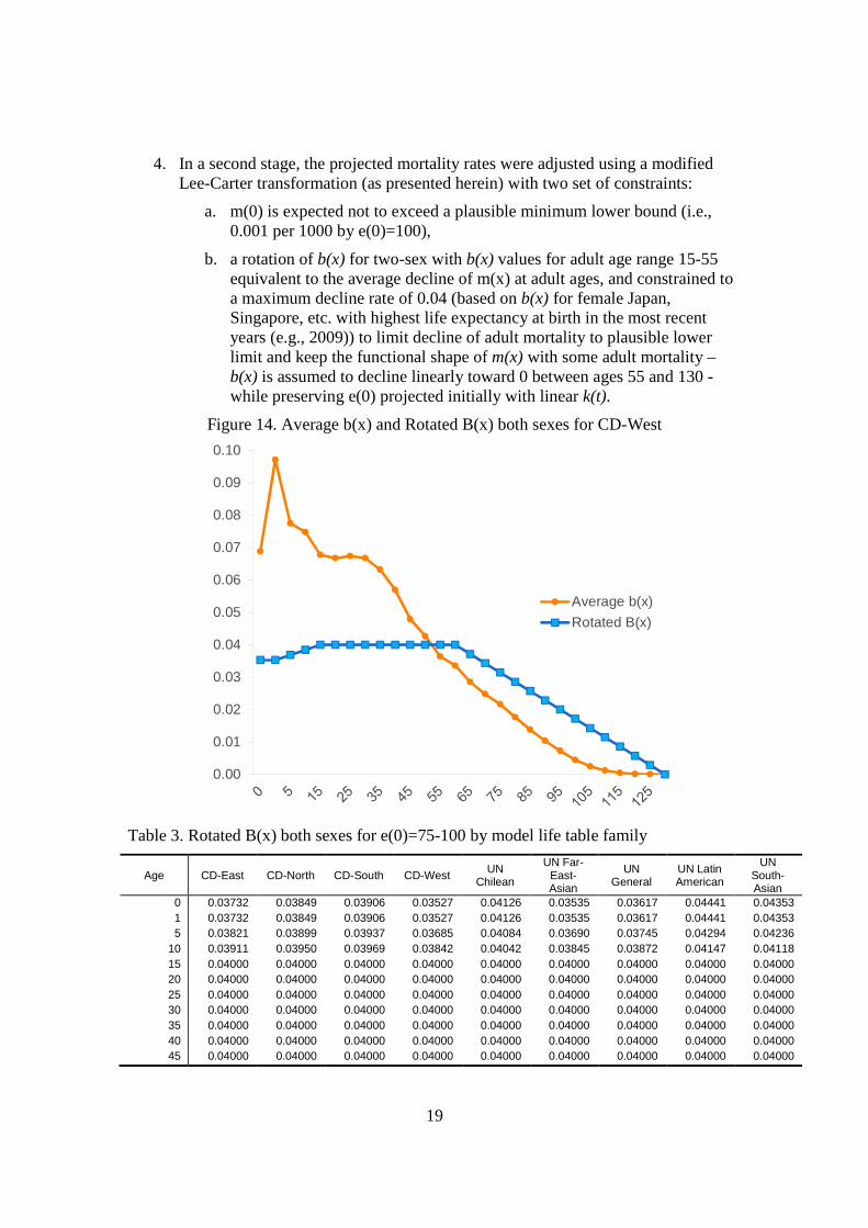
4. In a second stage, the projected mortality rates were adjusted using a modified Lee-Carter transformation (as presented herein) with two set of constraints:

a. m(0) is expected not to exceed a plausible minimum lower bound (i.e., 0.001 per 1000 by e(0)=100),

b. a rotation of b(x) for two-sex with b(x) values for adult age range 15-55 equivalent to the average decline of m(x) at adult ages, and constrained to a maximum decline rate of 0.04 (based on b(x) for female Japan, Singapore, etc. with highest life expectancy at birth in the most recent years (e.g., 2009)) to limit decline of adult mortality to plausible lower limit and keep the functional shape of m(x) with some adult mortality – b(x) is assumed to decline linearly toward 0 between ages 55 and 130 - while preserving e(0) projected initially with linear k(t).

Figure 14. Average b(x) and Rotated B(x) both sexes for CD-West

0.00

0.01

0.02

0.03

0.04

0.05

0.06

0.07

0.08

0.09

0.10

Average b(x)

Rotated B(x)

Table 3. Rotated B(x) both sexes for e(0)=75-100 by model life table family

Age CD-East CD-North CD-South CD-West UN Chilean

UN Far-East-Asian

UN General

UN Latin American

UN South-Asian

0 0.03732 0.03849 0.03906 0.03527 0.04126 0.03535 0.03617 0.04441 0.04353 1 0.03732 0.03849 0.03906 0.03527 0.04126 0.03535 0.03617 0.04441 0.04353 5 0.03821 0.03899 0.03937 0.03685 0.04084 0.03690 0.03745 0.04294 0.04236

10 0.03911 0.03950 0.03969 0.03842 0.04042 0.03845 0.03872 0.04147 0.04118 15 0.04000 0.04000 0.04000 0.04000 0.04000 0.04000 0.04000 0.04000 0.04000 20 0.04000 0.04000 0.04000 0.04000 0.04000 0.04000 0.04000 0.04000 0.04000 25 0.04000 0.04000 0.04000 0.04000 0.04000 0.04000 0.04000 0.04000 0.04000 30 0.04000 0.04000 0.04000 0.04000 0.04000 0.04000 0.04000 0.04000 0.04000 35 0.04000 0.04000 0.04000 0.04000 0.04000 0.04000 0.04000 0.04000 0.04000 40 0.04000 0.04000 0.04000 0.04000 0.04000 0.04000 0.04000 0.04000 0.04000 45 0.04000 0.04000 0.04000 0.04000 0.04000 0.04000 0.04000 0.04000 0.04000

20

Age CD-East CD-North CD-South CD-West UN Chilean

UN Far-East-Asian

UN General

UN Latin American

UN South-Asian

50 0.04000 0.04000 0.04000 0.04000 0.04000 0.04000 0.04000 0.04000 0.04000 55 0.04000 0.04000 0.04000 0.04000 0.04000 0.04000 0.04000 0.04000 0.04000 60 0.04000 0.04003 0.04001 0.04000 0.04000 0.04000 0.04000 0.04000 0.04000 65 0.03715 0.03720 0.03715 0.03714 0.03715 0.03715 0.03715 0.03715 0.03715 70 0.03430 0.03438 0.03430 0.03429 0.03429 0.03429 0.03429 0.03429 0.03429 75 0.03144 0.03155 0.03145 0.03143 0.03144 0.03143 0.03143 0.03144 0.03143 80 0.02859 0.02873 0.02860 0.02858 0.02858 0.02858 0.02858 0.02858 0.02858 85 0.02573 0.02590 0.02574 0.02572 0.02573 0.02572 0.02572 0.02572 0.02572 90 0.02288 0.02307 0.02289 0.02286 0.02287 0.02287 0.02287 0.02287 0.02287 95 0.02003 0.02025 0.02004 0.02001 0.02001 0.02001 0.02001 0.02001 0.02001

100 0.01717 0.01742 0.01719 0.01715 0.01716 0.01715 0.01715 0.01716 0.01716 105 0.01432 0.01460 0.01434 0.01430 0.01430 0.01430 0.01430 0.01430 0.01430 110 0.01147 0.01177 0.01148 0.01144 0.01145 0.01144 0.01144 0.01145 0.01144 115 0.00861 0.00894 0.00863 0.00858 0.00859 0.00859 0.00859 0.00859 0.00859 120 0.00576 0.00612 0.00578 0.00573 0.00574 0.00573 0.00573 0.00574 0.00573 125 0.00290 0.00329 0.00293 0.00287 0.00288 0.00288 0.00287 0.00288 0.00288 130 0.00005 0.00047 0.00008 0.00002 0.00003 0.00002 0.00002 0.00003 0.00002

Figure 15. Rotated B(x) both sexes for e(0)=75-100 by model life table family

0.00000

0.00500

0.01000

0.01500

0.02000

0.02500

0.03000

0.03500

0.04000

0.04500

0.05000

0 20 40 60 80 100 120

CD-East

CD-North

CD-South

CD-West

UN Chilean

UN Far-East-Asian

UN General

UN Latin American

UN South-Asian

Table 4. m(0) both sexes per 1000 by model life table family for selected level of e(0)

CD-East CD-North CD-South CD-West UN Chilean

UN Far-

East-Asian

UN

General

UN Latin

American

UN South-

Asian

e(0)=75 17.89 18.96 36.84 14.88 32.58 16.32 24.92 29.42 32.89

e(0)=100 0.36 0.60 0.67 0.42 1.02 0.70 0.99 0.66 0.78

5. A lowess smoother (alpha=0.2) was applied to the new series of m(x) by e(0) level to insure a smooth transition across the whole range of e(0) from 20 to 100, and to remove problems with Coale-Guo extension at younger ages for advanced e(0) compared to the Human Mortality Database experience.

21

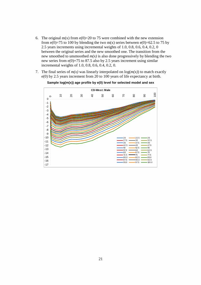
6. The original m(x) from e(0)=20 to 75 were combined with the new extension from e(0)=75 to 100 by blending the two m(x) series between e(0)=62.5 to 75 by 2.5 years increments using incremental weights of 1.0, 0.8, 0.6, 0.4, 0.2, 0 between the original series and the new smoothed one. The transition from the new smoothed to unsmoothed m(x) is also done progressively by blending the two new series from e(0)=75 to 87.5 also by 2.5 years increment using similar incremental weights of 1.0, 0.8, 0.6, 0.4, 0.2, 0.

7. The final series of m(x) was linearly interpolated on log(m(x)) to match exactly e(0) by 2.5 years increment from 20 to 100 years of life expectancy at birth.

Sample log(m(x)) age profile by e(0) level for selected model and sex

CD-West: Male

-17

-16-15

-14

-13-12

-11

-10-9

-8-7

-6

-5-4

-3

-2-1

0

0 10 20 30 40 50 60 70 80 90 100

20 22.5 2527.5 30 32.535 37.5 4042.5 45 47.550 52.5 5557.5 60 62.565 67.5 7072.5 75 77.580.0 82.5 85.087.5 90.0 92.595.0 97.5 100.0

22

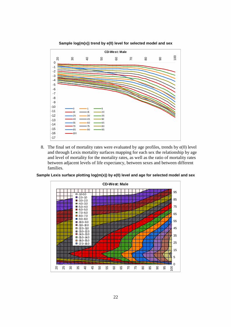
Sample log(m(x)) trend by e(0) level for selected model and sex

CD-West: Male

-17

-16-15

-14-13

-12

-11-10

-9-8

-7-6

-5

-4-3

-2-1

0

20 30 40 50 60 70 80 90 100

0 1 5

10 15 20

25 30 35

40 45 50

55 60 65

70 75 80

85 90 95

100

8. The final set of mortality rates were evaluated by age profiles, trends by e(0) level and through Lexis mortality surfaces mapping for each sex the relationship by age and level of mortality for the mortality rates, as well as the ratio of mortality rates between adjacent levels of life expectancy, between sexes and between different families.

Sample Lexis surface plotting log(m(x)) by e(0) level and age for selected model and sex

20 25 30 35 40 45 50 55 60 65 70 75 80 85 90 95 100

0

5

15

25

35

45

55

65

75

85

95

CD-West: Male

-1.0-0.0-2.0--1.0-3.0--2.0-4.0--3.0-5.0--4.0-6.0--5.0-7.0--6.0-8.0--7.0-9.0--8.0-10.0--9.0-11.0--10.0-12.0--11.0-13.0--12.0-14.0--13.0-15.0--14.0-16.0--15.0-17.0--16.0

23

Lexis surfaces plotting log(ratio of Mx between adjacent levels) by level and age for each model and sex

20 25 30 35 40 45 50 55 60 65 70 75 80 85 90 95

0

5

15

25

35

45

55

65

75

85

95

CD-West: Male

0.18-0.280.08-0.18-0.02-0.08-0.12--0.02-0.22--0.12-0.32--0.22-0.42--0.32-0.52--0.42-0.62--0.52-0.72--0.62-0.82--0.72-0.92--0.82-1.02--0.92-1.12--1.02

Sample Lexis surface plotting log(ratio of Mx for Male/Female) by level and age

for selected model

20 25 30 35 40 45 50 55 60 65 70 75 80 85 90 95 100

0

5

15

25

35

45

55

65

75

85

95

CD-West: Male/Female

1.6-1.81.4-1.61.2-1.41.0-1.20.8-1.00.6-0.80.4-0.60.2-0.40.0-0.2-0.2-0.0-0.4--0.2-0.6--0.4-0.8--0.6-1.0--0.8-1.2--1.0-1.4--1.2

24

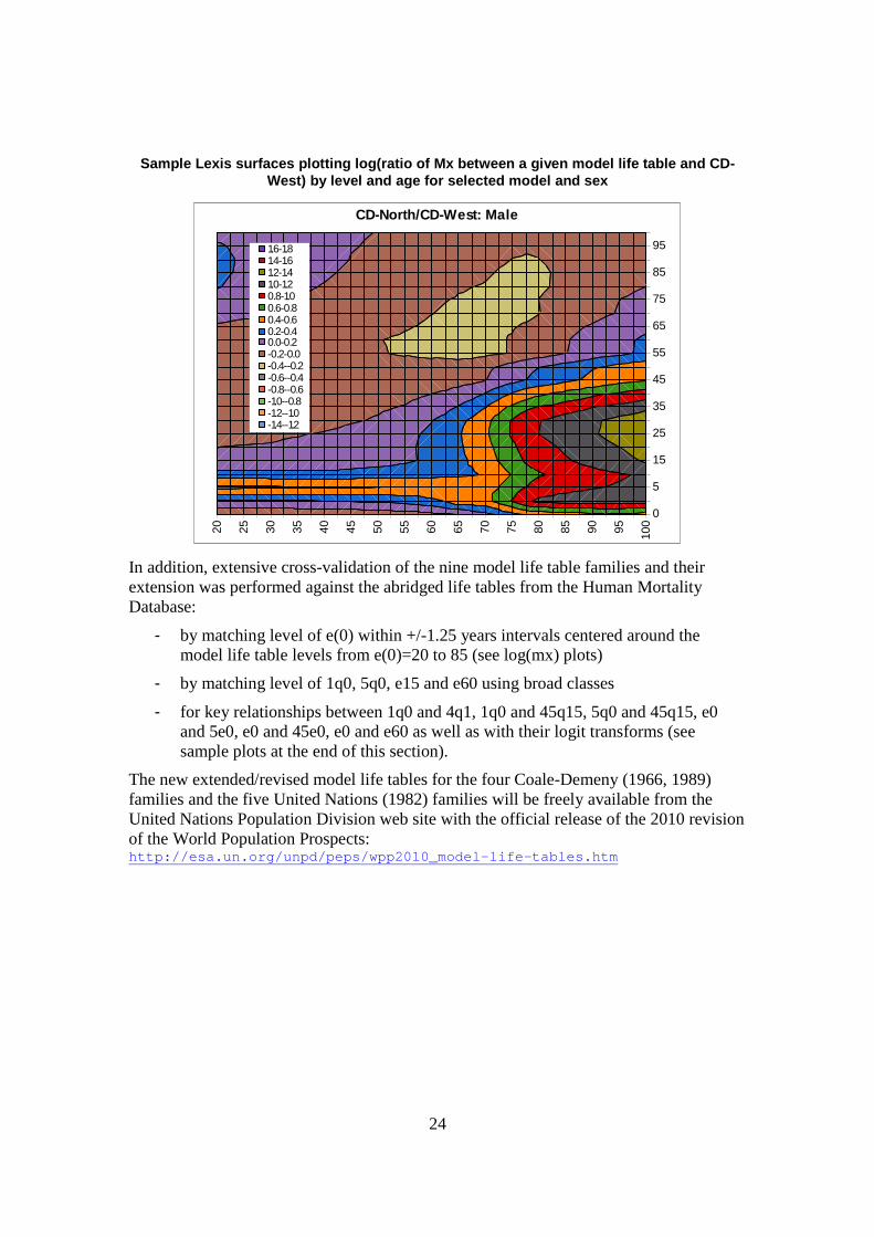
Sample Lexis surfaces plotting log(ratio of Mx between a given model life table and CD-West) by level and age for selected model and sex

20 25 30 35 40 45 50 55 60 65 70 75 80 85 90 95 100

0

5

15

25

35

45

55

65

75

85

95

CD-North/CD-West: Male

1.6-1.81.4-1.61.2-1.41.0-1.20.8-1.00.6-0.80.4-0.60.2-0.40.0-0.2-0.2-0.0-0.4--0.2-0.6--0.4-0.8--0.6-1.0--0.8-1.2--1.0-1.4--1.2

In addition, extensive cross-validation of the nine model life table families and their extension was performed against the abridged life tables from the Human Mortality Database:

- by matching level of e(0) within +/-1.25 years intervals centered around the model life table levels from e(0)=20 to 85 (see log(mx) plots)

- by matching level of 1q0, 5q0, e15 and e60 using broad classes

- for key relationships between 1q0 and 4q1, 1q0 and 45q15, 5q0 and 45q15, e0 and 5e0, e0 and 45e0, e0 and e60 as well as with their logit transforms (see sample plots at the end of this section).

The new extended/revised model life tables for the four Coale-Demeny (1966, 1989) families and the five United Nations (1982) families will be freely available from the United Nations Population Division web site with the official release of the 2010 revision of the World Population Prospects: http://esa.un.org/unpd/peps/wpp2010_model-life-tables.htm

25

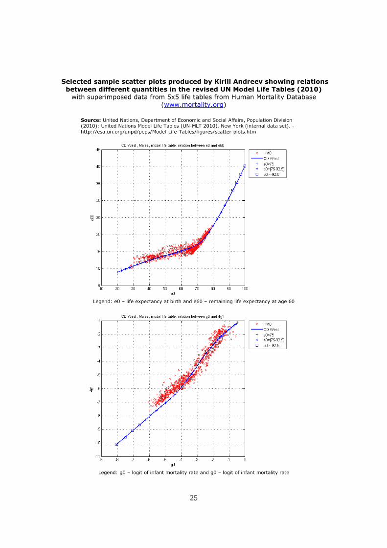
Selected sample scatter plots produced by Kirill Andreev showing relations

between different quantities in the revised UN Model Life Tables (2010)

with superimposed data from 5x5 life tables from Human Mortality Database

(www.mortality.org)

Source: United Nations, Department of Economic and Social Affairs, Population Division (2010): United Nations Model Life Tables (UN-MLT 2010). New York (internal data set). -

http://esa.un.org/unpd/peps/Model-Life-Tables/figures/scatter-plots.htm

Legend: e0 – life expectancy at birth and e60 – remaining life expectancy at age 60

Legend: g0 – logit of infant mortality rate and g0 – logit of infant mortality rate

26

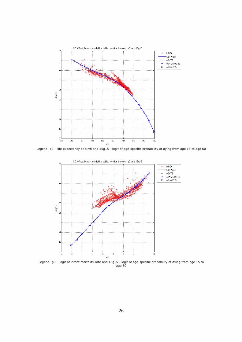
Legend: e0 – life expectancy at birth and 45g15 - logit of age-specific probability of dying from age 15 to age 60

Legend: g0 – logit of infant mortality rate and 45g15 - logit of age-specific probability of dying from age 15 to

age 60

4/6/2011

1

Modifying the Lee-Carter method to project mortality changes up to 2100

for all the 196 countries and areas with 100 thousand or more population in 2009with or without accurate, sufficient and regular data on ASDR.

Nan Li and Patrick GerlandUnited Nations Population Division. Department for Economic and Social Affairs, United Nations, New York, NY 10017, USA.

The views expressed in this paper are those of the authors and do not necessarily reflect those of the United Nations.

Population Association of America 2011 Annual Meeting - Washington, DC. Session 125: Formal Demography I: Mathematical Models and Methods (Friday 1 April 2011, 12:30 PM - 2:20 PM)

Outline

• Background context• Rotation model• Application to individual

and group of countries and issues• Robust Rotation• Application: Italy and Rep. of Korea,

(and in paper: Japan and extended model life tables up to e(0)=100)

2

4/6/2011

2

1. BACKGROUND CONTEXT

Why do we choose the Lee-Carter method?

[ ]

( )

(0)

log[ ( , )] ( , ),

log[ (0,1) ... log[ (0, )

... ... ...

log[ ( ,1) ... log

( )

(0)

..

[ ( , )

,

... (0)

... ... ...

( ) ... (

( )

(0) ... ( )

( ) ( 1) ( ( ) ~ ()

()

.

)

m b x

b

k t

k k T

k t

x t x

b

a x

a a

a

k t d e t

t

m m T

m n m n bT

e

n

t N

n a

σ

ε

= + +

= − +

≈ +

+

log[ (0, )]

..

0,1), ( ( )

.

log

(0)

...

( )

( )) 0

log[ (0, )

[ ( , )

]

...

log[ ( , )]

( ) ( )}

]

{

m T

m

E e s e t

m t

m n t

k t

n

k

T

b

b

T

n

=

= +

−

Why do we need to modify the Lee-Carter method?(1)Using “historical” b(x) and m(x,0,T) and adjusting k(t), we can fit any

value of e(t), the life expectancy at time t. Thus, stochastic projections of e(t) (Chunn et al, 2010) are transformed into stochastic projections of m(x,t) which can be used for stochastic population projections for all countries and areas of the world.

(2) To have reasonable age structure of projected m(x,t), several issues mostly related to constant b(x) must be addressed…

a(x) = most recent age pattern log(m(x))

b(x) = rate of change by age groups

k(t) = overall time trend

4/6/2011

3

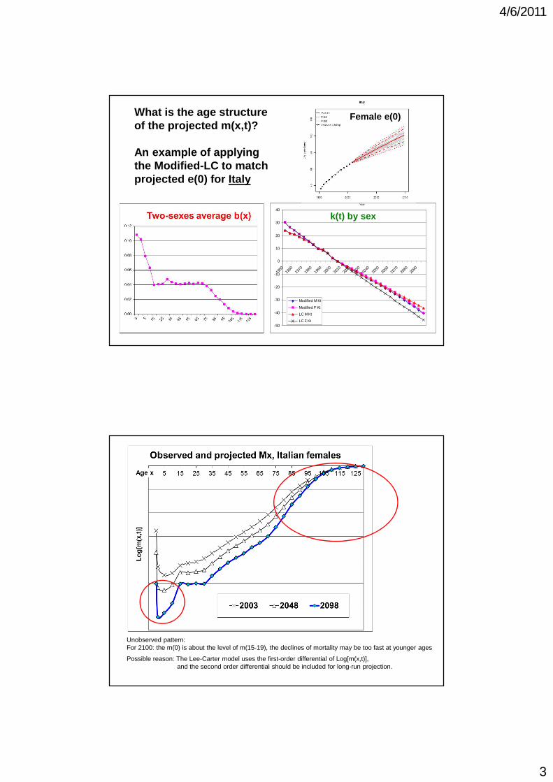
What is the age structure of the projected m(x,t)?

An example of applying the Modified-LC to match projected e(0) for Italy

-50

-40

-30

-20

-10

0

10

20

30

40

1950

1960

1970

1980

1990

2000

2010

2020

2030

2040

2050

2060

2070

2080

2090

Modified M Kt

Modified F Kt

LC M Kt

LC F Kt

Female e(0)

k(t) by sex

Unobserved pattern:For 2100: the m(0) is about the level of m(15-19), the declines of mortality may be too fast at younger ages

Possible reason: The Lee-Carter model uses the first-order differential of Log[m(x,t)], and the second order differential should be included for long-run projection.

4/6/2011

4

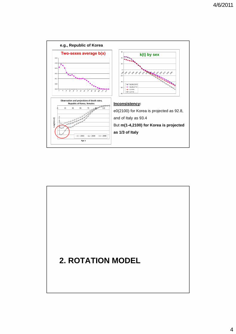
e.g., Republic of Korea

-80

-60

-40

-20

0

20

40

60

1950

1960

1970

1980

1990

2000

2010

2020

2030

2040

2050

2060

2070

2080

2090

Modif ied M Kt

Modif ied F Kt

LC M Kt

LC F Kt

Observation and projections of death rates, Republic of Korea, females

-5 15 35 55 75 95 115

Age x

Lo

g[m

(x,t

)]

2003 2048 2098

Inconsistency:

e0(2100) for Korea is projected as 92.8,

and of Italy as 93.4

But m(1-4,2100) for Korea is projected

as 1/3 of Italy

k(t) by sex

2. ROTATION MODEL

4/6/2011

5

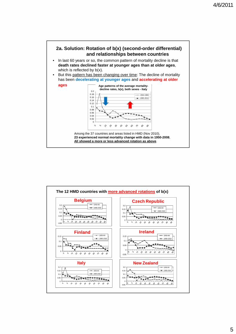
2a. Solution: Rotation of b(x) (second-order differential)and relationships between countries

• In last 60 years or so, the common pattern of mortality decline is that death rates declined faster at younger ages than at older ages, which is reflected by b(x).

• But this pattern has been changing over time: The decline of mortality has been decelerating at younger ages and accelerating at older ages

Figure 1. Age patterns of the average mortality-decline rates, two-sex combined, Italy

0

0.02

0.04

0.06

0.08

0.1

0.12

0.14

0.16

0.18

0.2

0 5 15

25

35

45

55

65

75

85

95

1950-1980

1980-2010

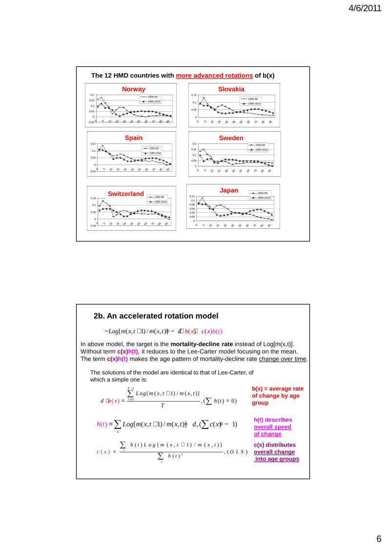
Among the 37 countries and areas listed in HMD (Nov 2010), 23 experienced normal mortality change with data in 1950-2008, All showed a more or less advanced rotation as above.

Age patterns of the average mortality-decline rates, b(x), both sexes - Italy

-0.05

0

0.05

0.1

0.15

0.2

Belgium1950-80

1980-2010

0

0.05

0.1

0.15

0.2

Czech Republic1950-80

1980-2010

0

0.05

0.1

0.15

Finland1950-80

1980-2010

-0.05

0

0.05

0.1

0.15

Ireland1950-80

1980-2010

0

0.05

0.1

0.15

0.2

Italy

1950-80

1980-2010

-0.05

0

0.05

0.1

0.15

0.2

New Zealand1950-80

1980-2010

The 12 HMD countries with more advanced rotations of b(x)

4/6/2011

6

Norway

-0.05

0

0.05

0.1

0.15

0.2

0 5 15 25 35 45 55 65 75 85 95

1950-80

1980-2010

Slovakia

0

0.05

0.1

0.15

0 5 15 25 35 45 55 65 75 85 95

1950-80

1980-2010

Spain

-0.05

0

0.05

0.1

0.15

0 5 15 25 35 45 55 65 75 85 95

1950-80

1980-2010

Sweden

0

0.05

0.1

0.15

0.2

0 5 15 25 35 45 55 65 75 85 95

1950-80

1980-2010

Switzerland

-0.05

0

0.05

0.1

0.15

0 5 15 25 35 45 55 65 75 85 95

1950-80

1980-2010

Japan

0

0.02

0.04

0.06

0.08

0.1

0.12

0 5 15 25 35 45 55 65 75 85 95

1950-80

1980-2010

The 12 HMD countries with more advanced rotations of b(x)

Norway

Spain

Switzerland Japan

Sweden

Slovakia

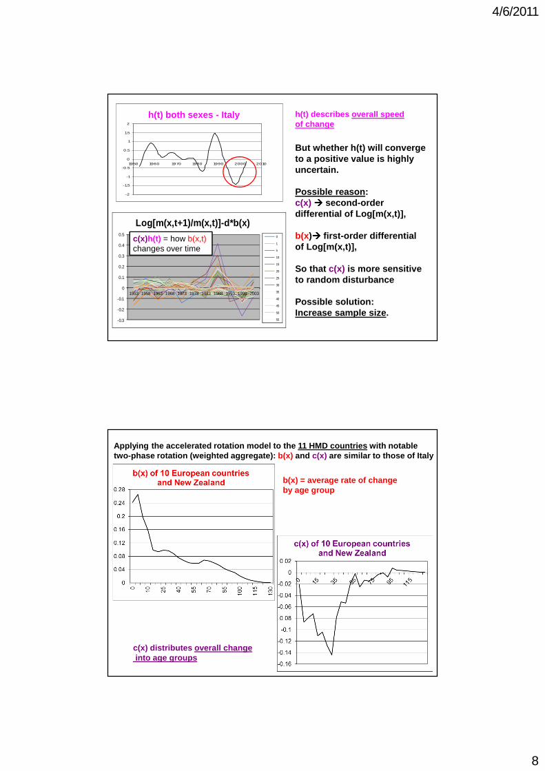
2b. An accelerated rotation model

[ ( , 1) / ( , ) ( )) ( )] (Log m x t m x t d c x hb x t− + = − ⋅ +

In above model, the target is the mortality-decline rate instead of Log[m(x,t)]. Without term c(x)h(t), it reduces to the Lee-Carter model focusing on the mean. The term c(x)h(t) makes the age pattern of mortality-decline rate change over time.

The solutions of the model are identical to that of Lee-Carter, of which a simple one is:

1

0

[ ( , 1( )

) / ( , )], ( ( ) 0)

T

t

L og m x t m x td h tb x

T

−

=

+⋅ = =

∑∑

[ ( , 1) / ( , )] , ( ( ) 1)( )x

Log m x t m x t d c xh t = + − = −∑ ∑

2

( ) [ ( , 1 ) / ( , ) ], ( )

()

)( t

t

h t L o g m x t m x tO L S

hc x

t

+=∑

∑

h(t) describes overall speed of change

c(x) distributes overall changeinto age groups

b(x) = average rate of change by age group

4/6/2011

7

3. ROTATION MODEL: APPLICATION

Figure 3.1. The b(x) of Italy

-0.04

0

0.04

0.08

0.12

0.16

0.2

0.24

0.28

0.32

0 10 25 40 55 70 85 100

115

130

Figure 3.2. The c(x) of Italy

-0.18

-0.16

-0.14

-0.12

-0.1

-0.08

-0.06

-0.04

-0.02

0

0 10 25 40 55 70 85 100

115

130 c(x) shape looks plausible

If h(t) converges to a positive value:Mortality-decline rate will be reduced more at young ages.

b(x) is identical to the Lee-Carter version

c(x) distributes overall changeinto age groups

b(x) = average rate of change by age group

b(x) both sexes - Italy

c(x) both sexes - Italy

4/6/2011

8

Figure 3.3 The h(t) of Italy

-2

-1.5

-1

-0.5

0

0.5

1

1.5

2

1950 1960 1970 1980 1990 2000 2010

-0.3

-0.2

-0.1

0

0.1

0.2

0.3

0.4

0.5

1953 1958 1963 1968 1973 1978 1983 1988 1993 1998 2003

Log[m(x,t+1)/m(x,t)]-d*b(x)0

1

5

10

15

20

25

30

35

40

45

50

55

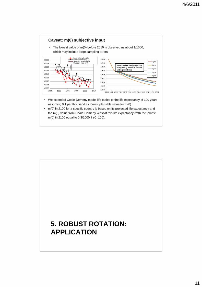
But whether h(t) will converge to a positive value is highly uncertain.

Possible reason:c(x) ���� second-order differential of Log[m(x,t)],

b(x)���� first-order differential of Log[m(x,t)],

So that c(x) is more sensitive to random disturbance

Possible solution:Increase sample size.

h(t) describes overall speed of change

h(t) both sexes - Italy

c(x)h(t) = how b(x,t)changes over time

Applying the accelerated rotation model to the 11 HMD countries with notable two-phase rotation (weighted aggregate): b(x) and c(x) are similar to those of Italy

c(x) distributes overall changeinto age groups

b(x) = average rate of change by age group

4/6/2011

9

Log[m(x,t+1)/m(x,t)]-d*b(x)

-0.3

-0.2

-0.1

0

0.1

0.2

0.3

0.4

1953 1958 1963 1968 1973 1978 1983 1988 1993 1998 2003

015101520253035404550556065707580859095100105110115120125130

But h(t) for these 11 HMD countries is smoother and looks more certain to converge to a positive value

h(t) describes overall speed of change in b(x,t)

c(x)h(t) = how b(x,t)changes over time

Using the potential converging levels of h(t), the rotated b(x)looks plausible at age 15 and over.

At ages younger than 15, the rotation may be still premature.

Figure 6. Age patterns of the average mortality-decline rates, tw o-sex combined, 11 countries

0

0.02

0.04

0.06

0.08

0.1

0.12

0.14

0.16

0.18

0 5 15 25 35 45 55 65 75 85 95

1950-1980

1980-2010

We conclude that we cannot establish a data-driven rotation model now.We turn to a rotation model based on subjectively inputting ultimate m(0).

Observed b(x), 11 HMD countries

4/6/2011

10

4. ROBUST ROTATION MODEL

This subjective model is based on the following assumptions:1. At adult ages (15-60), B(x) is the average of b(x) over these ages;2. At old ages, B(x) is the linear interpolation between that at ages 55-60

and at the oldest age of the model;3. At young ages, B(0) is a subjective input,

B(1-4)=B(0) and other B(x) are linear interpolations between B(1-4) and B(15-19).

The robust rotation model B(x)

B(0) is determined by fitting an ultimate m(0), just like k(t) can be adjusted to fit e0(t).

12

3

4/6/2011

11

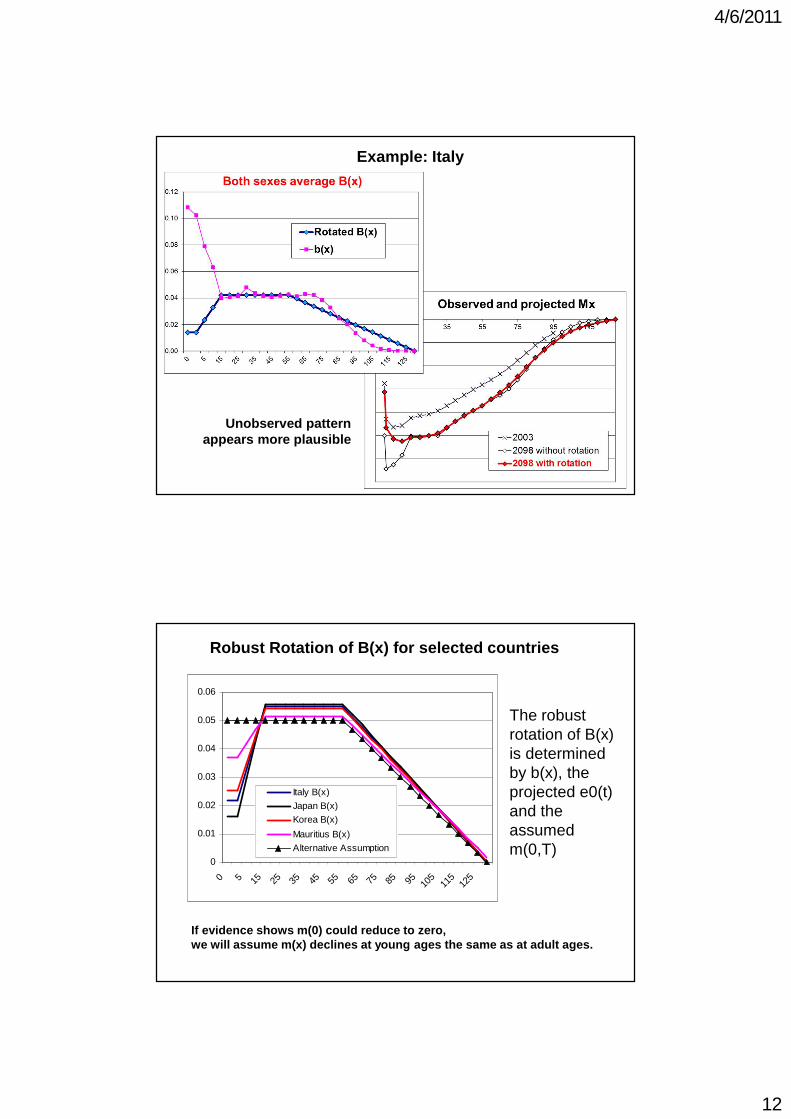
Caveat: m(0) subjective input

• The lowest value of m(0) before 2010 is observed as about 1/1000, which may include large sampling errors.

• We extended Coale-Demeny model life tables to the life expectancy of 100 years assuming 0.1 per thousand as lowest plausible value for m(0)

• m(0) in 2100 for a specific country is based on its projected life expectancy and the m(0) value from Coale-Demeny West at this life expectancy (with the lowest m(0) in 2100 equal to 0.3/1000 if e0=100).

0.0005

0.0015

0.0025

0.0035

0.0045

0.0055

0.0065

0.0075

0.0085

1985 1990 1995 2000 2005 2010

Iceland female m(0) Iceland male m(0)Sw eden female m(0)Sw eden male m(0)

Japan female m(0) projection using AR(3) model of decline and n-period data

5. ROBUST ROTATION: APPLICATION

4/6/2011

12

Example: Italy

Unobserved pattern appears more plausible

The robust rotation of B(x) is determined by b(x), the projected e0(t) and the assumed m(0,T)

0

0.01

0.02

0.03

0.04

0.05

0.06

0 5 15 25 35 45 55 65 75 85 95 105

115

125

Italy B(x)

Japan B(x)

Korea B(x)

Mauritius B(x)

Alternative Assumption

If evidence shows m(0) could reduce to zero, we will assume m(x) declines at young ages the same as at adult ages.

Robust Rotation of B(x) for selected countries

4/6/2011

13

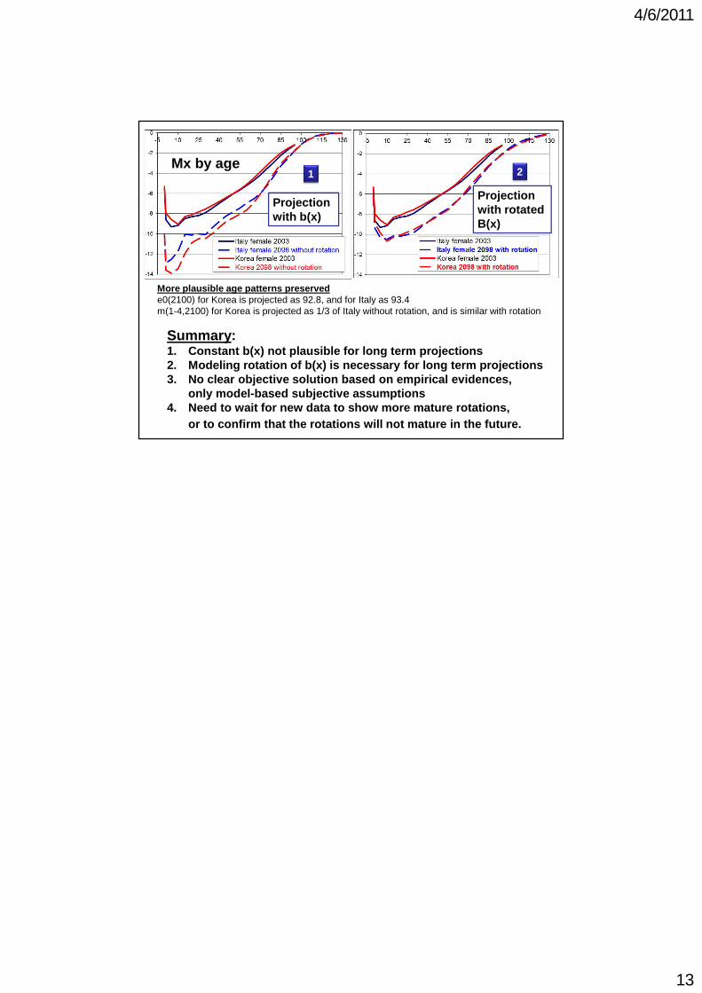
More plausible age patterns preservede0(2100) for Korea is projected as 92.8, and for Italy as 93.4m(1-4,2100) for Korea is projected as 1/3 of Italy without rotation, and is similar with rotation

Summary:1. Constant b(x) not plausible for long term projections2. Modeling rotation of b(x) is necessary for long term projections3. No clear objective solution based on empirical evidences,

only model-based subjective assumptions4. Need to wait for new data to show more mature rotations,

or to confirm that the rotations will not mature in the future.

1 2Mx by age

Projection with rotated B(x)

Projection with b(x)