Name: ___________________________________Period____Date________________

ESS 101: UW in the HS, Mercer Island High School

Lab – Topographic Maps

Introduction and instructional material are from Dr. Terry Swanson, University of

Washington, Dr. David Kendrick, Hobart and William Smith Colleges, Geneva, NY,

the US Geological Survey, and the Science Education and Research Consortium

(serc.carleton.edu).

Geoscientists utilize many different techniques to study the Earth. Many of these techniques do not

always involve fieldwork or direct sampling of the earth’s surface. Before a geoscientist completes work

in the field he or she will often review maps or remote images to provide important information relevant

to a given study area. For example, when a geoscientist is retained to assess landslide hazards for a

proposed housing development located proximal to a steep bluff slope, he or she would certainly want to

review topographic maps, geologic substrate maps, and aerial photography prior to completing a field

visit to the study area. Since topography and substrate geology play important roles in landslide

processes, it is important for a geoscientist to review the slope conditions and the underlying substrate

geology to better understand potential landslide hazards for a given study area. Aerial photography, or

other remote imagery, may provide the geoscientist with important historical data, such as vegetation age

structure or other evidence quantifying the frequency of landslide activity and related hillslope erosion.

Geoscientists also utilize maps and remote imagery to record their field data so that it can be synthesized

and interpreted within a spatial context and shared with other geoscientists or the general public.

In today’s laboratory we will explore map-reading techniques that are utilized by geoscientists to study

the geologic landscapes and processes operating at Earth’s surface. Many of these techniques will be

integrated into future laboratory exercises.

Goals – your goals in this lab are twofold. 1) Understand how a topographic map represents the

Earth’s surface and be able to create and interpret such a map. 2) Solve problems using published

topographic maps and your newly discovered map-reading abilities.

BACKGROUND INFORMATION

History of Maps A map is a two-dimensional representation of a portion of the Earth’s surface. Maps have been used by

ancient and modern civilizations for over three thousand years. The Egyptians, Ancient Greeks, Babylonians

and Roman civilizations drew the earliest recorded maps. These earliest maps were largely drawn to denote

place names and general directions, often neglecting accuracy and scale. Figures 1-1A and 1-1B illustrate the

simplicity of these early maps.

Name: ___________________________________Period____Date________________

Figures 1-1A and 1-1B: Babylonian map of the world (Fig. 1-1A) drawn on a clay tablet circa 500 B.C. The map represents

ancient Babylon, the Euphrates River and surrounding ocean, which today comprises modern Iraq. Fig. 1-1B is a representation

of an original Roman map entitled, Orbis Terrarum, drawn by Marcus Vipsanius Agrippa in 20 A.D. The ancient Roman map

shows Europe, Asia and Africa surrounding the Mediterranean Sea.

Figure 1-1A taken from History of Cartography Volume One: Cartography in Prehistoric, Ancient, and Medieval Europe and

the Mediterranean. Edited by J. B. Harley and David Woodward (1987), The University of Chicago Press, Chicago and London.

Figure 1-1B redrawn from Erwin Raisz, 1948. General Cartography. McGraw Hill.

Following the decline of the Roman Empire, near the end of the 5th

century A.D., innovation and

advancement in cartography declined for almost 1000 years until the start of the Renaissance Period in the

late 14th

century. During the Renaissance Period the Age of Exploration and Discovery brought about a need

for increased accuracy in maps, particularly for navigational purposes as global trade and colonization

increased. Figure 1-2 shows a world map, originally published by the Flemish cartographer Gerard Mercator

in 1595, and subsequently published in Henricus Hondius’ Atlas in 1633 (image taken from the U.S. Library

of Congress web site. An Illustrated Guide Geography and Maps., URL:

www.loc.gov/rr/geogmap/guide/gmillatl.html). Such maps provided valuable navigational information,

such as latitude and longitude coordinates and the seasonal position of the overhead sun for sea faring

explorers and traders.

Figure 1-2: Hondius’ map of the world was depicted in two hemispheres bordered by the representation of the four elements of

fire, air, water and land. Portraits of the Roman Emperor Julius Caesar, Claudius Ptolemy, a 2nd

century A.D. geographer,

and the atlas’s first two publishers, Mercator and Hondius also adorn the map’s border.

Name: ___________________________________Period____Date________________

Over the subsequent 500 years the accuracy and detail of maps has improved greatly with technological

advances in surveying equipment and the advent of aerial and satellite imagery. Most maps used today are

planometric, which convey data on a two-dimensional surface (Figure 1-3). Planometric maps may provide

information about transportation routes, geographic location, nominal data, vegetation patterns or other

forms of data requiring spatial representation.

Location Latitude and Longitude

Most maps have a geographic coordinate grid, which can be used to determine location. The most

commonly used coordinate system is latitude and longitude. Latitude is an angular distance measured

north or south of the Earth’s equator, which is 0° latitude. It varies from 0° to 90° north and from 0° to

90° south (Figure 1-4). Lines of latitude encircle the Earth parallel to the equator and are called parallels

because they are parallel to one another. Lines of longitude represent the angular distance measured east

or west from the prime meridian (0° longitude), which passes through the Royal Astronomical

Observatory in Greenwich, England. Lines of longitude range from 0° to 180° east and 0° to 180° west

(Figure 1-4). The international date line is the line represented by both 180° east and 180° west

longitude. Lines of longitude are termed meridians and encircle the Earth in a direction perpendicular to

the equator. Meridians of longitude converge at the North and South poles; thus, they are neither parallel

nor equally spaced except along a given line of latitude. Ground distance represented by a degree or

minute of longitude decreases poleward from the equator because of this convergence.

Name: ___________________________________Period____Date________________

Units of latitude and longitude are expressed in degrees (°), and further subdivided into minutes [60

minutes (') = one degree], and seconds (60 seconds ('') = one minute). For example, Seattle is located at

47°27'00'' N, 122°18'00'' W. To accurately convey a specific location on the earth’s surface, it is important

to state whether its latitude lies north or south of the equator and longitude lies east or west of the prime

meridian. By convention, a location’s latitude is stated first, followed by its longitude coordinate.

Figure 1-4: World globe showing latitude and longitude coordinates.

Topographic Maps

Maps are fundamental geological tools. We use maps to represent a host of information, including rock

distribution, water tables, and, most commonly, the shape of the Earth’s surface. Topography is the

shape of the Earth’s surface; maps that represent this surface are called topographic maps. Topographic

maps depict the Earth’s surface by means of contour lines, or lines of constant elevation.

Name: ___________________________________Period____Date________________

An Introduction to Topographic Maps

To use topographic maps, you need to understand several basic map features:

Location: Location information identifies the area covered by a map. United States Geological Survey

(USGS) maps cover rectangular areas and are identified by a quadrangle name. A state index map

shows the locations and names of all the quadrangles in a state and can be used to find the quadrangle

that covers a particular area. In addition to quadrangle names, USGS maps are marked with latitude and

longitude and other coordinate systems that can be used to locate a map area or feature relative to larger

geographic features.

Scale Map Scale: Maps are representations of an area. This means that the distance between two points on a

map corresponds to some true distance on the ground. The ratio of map distance to true distance is the

map scale. Most maps represent a reduced image of a larger area. The amount of reduction is defined by a

map’s scale and may be expressed in the following ways:

Graphic Scale: Scale is indicated by a calibrated bar or line. For example, the bar scale shown in Figure 1-5

represents a distance of two kilometers on the Earth’s surface.

Figure 1-5:

Most people are familiar with a map’s scale bar. A scale bar is a line or bar of some predetermined map

length, 2 cm for example, which is labeled with the corresponding true distance, for example, 2

kilometers.

Fractional Scale: Scale is expressed as a fixed ratio between a distance measured on a map and an equal

distance measured on the Earth’s surface. This ratio is termed the representative fraction. For example, a

fractional scale of 1:24,000 indicates that one distance unit on the map (inches, feet, centimeters, etc.) equals

24,000 of the same distance units on the surface of the Earth.

Verbal Scale: is used to verbally convey the map scale, but is rarely written on the map. For example, a

verbal scale of “1 inch equals 1 mile” represents a fractional scale of 1:63,360, as 63,360 inches equals one

mile.

Many topographic maps, for instance, have a scale of 1:24,000. This means that one cm on the map

equals 24,000 cm on the ground, one foot on the map equals 24,000 feet on the ground, etc. The scale

1:24,000 can also be expressed as a decimal fraction, 1/24000 =0.000041666. While scale bars are

handy for a rough approximation of lengths, fractional scales allow precise calculations of lengths. Two

equations are particularly useful:

True Distance = (Map Distance) * (Fractional Scale)

Map Distance = (True Distance) / (Fractional Scale)

Note: These expressions assume that map and true distances are expressed in the same units! Thus if you

Name: ___________________________________Period____Date________________

measure map distance in cm and calculate true distance, the calculated distance will be in cm. If true

distance is in miles and you calculate map distance, the calculated distance will be in miles.

Orientation: Most maps have a North arrow. When the map is oriented so that the North arrow on the

map points to north on the Earth, directions on the map are the same as directions on the ground and the

map can be used for navigation. In addition to showing true geographic North, USGS maps show

magnetic north. In most of Washington, the discrepancy is about 20o east; compass needles point to a

direction that is 20o east of due North. This “magnetic declination” changes with location—in the

eastern United States, magnetic declinations are west of due North. Besides North arrows, lines of

longitude and latitude or other similar coordinate systems can be used to orient a map.

Magnetic Declination

Figure 1-6: USGS magnetic declination symbol. The star represents geographic north, GN is grid north, and MN is magnetic

north. This symbol shows a magnetic declination of 16½°.

On the surface of the earth the magnetic north pole (where a compass needle will point) is not the same

location as the “true” or geographic north pole, which defines the earth’s axis of rotation. The angular

distance between geographic and magnetic north at a given location represents its magnetic declination.

Because magnetic declination varies over time and space, a symbol and explanation is provided on the lower

margin of most U.S. Geological Survey (USGS) topographic maps (Figure 1-6). This symbol shows the

magnetic declination for the center area of a topographic map at the time it was published or revised.

Within the conterminous United States, magnetic declination varies between 20° west in Maine and 20° east

in Washington (Figure 1-7). Up to date magnetic declination measurements provide important information in

order to determine accurate directions when mapping and navigating over large distances. Geoscientists and

Name: ___________________________________Period____Date________________

backpackers alike require accurate magnetic declination data to set their compasses appropriately when using

base maps.

Up to date declination data within the conterminous United States can be acquired using an online

declination calculator found on the National Geophysical Data Center’s (NGDC) web site:

www.ngdc.noaa.gov/geomagmodels/Declination.jsp Figure 1-7: Map of magnetic declination for the conterminous United States (U.S. Geological Survey).

Contour Lines Topographic maps are important tools used by earth scientists because they show the three-dimensional

configuration of the Earth’s surface by means of contour lines, which connect points of equal elevation.

Contour lines may be visualized as the intersection of a series of equally spaced, horizontal planes with the

Earth’s surface. The relationship between a topographic map and the land surface it represents is illustrated

in Figures 1-8 and 1-9

Name: ___________________________________Period____Date________________

Figure 1-8: Example of contour lines on a 3-dimensional block diagram.

.

Figure 1-9: Block diagram illustrating the relationship between a topographic map and the land surface it represents.

Name: ___________________________________Period____Date________________

There are some simple rules to follow when reading or constructing topographic maps. Figure 1-9

graphically illustrates how these rules apply to contour maps.

(1) Contour lines connect points of equal elevation.

(2) Contour lines do not cross (except in the rare case of an overhanging cliff).

(3) Contour lines never diverge.

(4) Contour lines do not end except at the edges of a map or by closing on themselves.

(5) The spacing of contour lines is related to the steepness of a slope: Widely spaced contour lines

characterize gentle slopes and closely spaced contour lines indicate steep slopes.

(6) A rounded hill is represented by a concentric series of closed contours.

(7) A “closed depression” is represented by a concentric series of closed contours that have hachure marks

(tick marks) on the downhill side.

(8) Contour lines form V's which point upstream when they cross stream valleys.

The vertical distance of separation between adjacent contour lines is called the contour interval. Selection

of a contour interval is a function of map scale and the extent of topographic variation within an area.

Typically, the greater the vertical relief that is represented on a map, the greater the contour interval. The

contour interval, shown at the bottom of the map, remains constant throughout the map area.

On most topographic maps, every fifth contour line is printed darker for easy recognition and is labeled with

its elevation. These index contours appear dark brown on U.S. Geological Survey topographic maps.

Intermediate contour lines are lighter brown and elevation data are not given. Elevations of intermediate

contour lines may be determined by interpolating between the nearest index contour and adding or

subtracting the appropriate elevation as determined by the map’s contour interval. If a point lies between two

contour lines, then its elevation must also be interpolated. Elevations of specific points (tops of peaks, survey

points, etc.) are sometimes indicated directly on the map. The notation "BM" denotes the location of a

benchmark, a permanent marker placed by the U.S. Geological Survey or other governmental agencies at

the point indicated on the map. Elevations are usually given for benchmarks.

Slope and Gradients

Topographic maps permit measurement of the slope, defined as the change in vertical distance divided by

the horizontal distance (rise over run). For example, to calculate the slope of a hill that has a vertical rise of

80 feet and a horizontal run of 800 feet:

Note that the units of measurement (in feet) cancel each other out; thus, the calculated slope is

dimensionless. To calculate the slope in degrees you would take arctangent of rise over the run and convert

radians to degrees.

Name: ___________________________________Period____Date________________

The gradient of a slope is most often expressed as a change in vertical height (measured in feet or meters)

compared to the horizontal length of the sloping surface (measured in miles or kilometers). Measurement of

the gradient requires accurate determination of elevations and effective use of map scales. For example, if

two separate points have elevations of 182 and 118 feet respectively, and are separated by a distance of 1.8

miles, the gradient between the two points may be calculated as follows:

Stream and river gradients may be calculated in a similar fashion; however, map distances must be measured

along stream channels, rather than as a straight line. This can be facilitated by using a piece of string and

measuring along the course of the stream channel.

Relief

Relief refers to the difference between the highest and lowest point in a given area. Relief can be expressed

either numerically (e.g. a mountain has 865 ft of relief above the valley floor), or in a relative sense (e.g. a

plain would have low relief while a mountain range would have high relief).

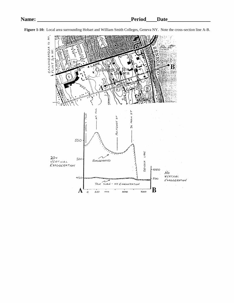
Topographic Profiles

To better visualize topography, it is often advantageous to construct a topographic profile, which

presents a "side-view," or cross-section, of the Earth's surface. Construction of a topographic profile is

not difficult if the following guidelines are followed:

(1) Place a strip of paper along a selected profile line

(2) Mark on the paper the exact location where each index contour line, hill crest, and valley crosses the

profile line. Label each mark with its elevation. For very steep topography, where contour lines are very

close together (e.g., a steep cliff), you may decide to only label the base of steep cliff and its top elevation

before continuing to label the index contours.

(3) Make a vertical grid on graph paper. The horizontal axis should show units of horizontal distance along

the profile line and be the same length as your profile line. The vertical axis should show elevation units

ranging from the lowest to highest points on your profile line.

(4) Place the paper strip above the vertical grid and project each marked topographic feature downward to its

proper elevation.

(5) Connect all the points on the grid with a smooth line, which is consistent with topographic trends. The

result is a silhouette of the topography along the profile line.

Name: ___________________________________Period____Date________________

Figure 1-10: Illustrations of how to make a topographic profile.

Map Symbols In the lower right corner of most U.S. Geological Survey (USGS) topographic maps, a legend is given that

shows a few of the important symbols used on the map. The USGS has adopted standardized map symbols

and color-coding to represent physiographic, cultural, and survey features shown on the map. A complete

list of these symbols can be found at: pubs.usgs.gov/gip/TopographicMapSymbols/topomapsymbols.pdf

Name: ___________________________________Period____Date________________

Figure 1-10: Local area surrounding Hobart and William Smith Colleges, Geneva NY. Note the cross-section line A-B.