Discussion Paper No. 1021

NAKED EXCLUSION UNDER

EXCLUSIVE-OFFER COMPETITION

Hiroshi Kitamura Noriaki Matsushima

Misato Sato

March 2018

The Institute of Social and Economic Research Osaka University

6-1 Mihogaoka, Ibaraki, Osaka 567-0047, Japan

Naked Exclusion under Exclusive-offer Competition∗

Hiroshi Kitamura† Noriaki Matsushima‡ Misato Sato§

March 2, 2018

Abstract

This study constructs a model of anticompetitive exclusive-offer competition be-

tween two existing upstream firms. Under exclusive-offer competition, the upstream

firm’s profit depends on the rival’s exclusive offer. If the rival makes an exclusive offer

acceptable for the downstream firm, the upstream firm is excluded unless it succeeds in

exclusion. Consequently, the upper bound of exclusive offers becomes higher than when

one of the upstream firms is a potential entrant that cannot make any exclusive offer.

Thus, the exclusion of the existing upstream firm can be an equilibrium outcome even in

the case where the potential entrant is never excluded.

JEL classification codes: L12, L41, L42.

Keywords: Antitrust policy; Exclusive dealing; Exclusive-offer competition; Imperfect com-

petition.

∗We thank Takanori Adachi, Masaki Aoyagi, Jay Pil Choi, Susumu Imai, Akifumi Ishihara, Atsushi Ka-

jii, Simon Loertscher, Toshihiro Matsumura, Stuart McDonald, Masao Ogaki, Johannes Paha, Jerome Pouyet,

Takeharu Sogo, and Zhiyong Yao as well as the conference participants at the 2nd Asia-Pacific Industrial Organ-

isation Conference (University of Auckland), 44th European Association for Research in Industrial Economics

Annual Conference (Maastricht University), 15th Annual International Industrial Organization Conference (Re-

naissance Boston Waterfront Hotel), and XXXII Jornadas de Economıa Industrial (Universidad de Navarra)

and seminar participants at Keio University, Kyoto Sangyo University, Osaka University, Sapporo Gakuin Uni-

versity, and Tohoku University. We gratefully acknowledge the financial support from JSPS KAKENHI grant

numbers JP15H03349, JP15H05728, JP15K17060, JP17H00984, JP17J03400, and JP17K13729. The usual

disclaimer applies.†Faculty of Economics, Kyoto Sangyo University, Motoyama, Kamigamo, Kita-Ku, Kyoto, Kyoto 603-8555,

Japan. E-mail: hiroshikitamura@cc.kyoto-su.ac.jp‡Institute of Social and Economic Research, Osaka University, 6-1 Mihogaoka, Ibaraki, Osaka 567-0047,

Japan. E-mail: nmatsush@iser.osaka-u.ac.jp§Postdoctoral Research Fellow of the Japan Society for the Promotion of Science (JSPS), Faculty of Eco-

nomics, Kyoto Sangyo University, Motoyama, Kamigamo, Kita-Ku, Kyoto, Kyoto 603-8555, Japan. E-mail:

smisato@gwmail.gwu.edu

1 Introduction

Exclusive contracts have been a controversial issue in competition policy because they are

seemingly anticompetitive due to the exclusion of rival firms. However, by taking into ac-

count all members’ participation constraints for such exclusive dealing in the contract party

under a one-seller-one-buyer framework, Posner (1976) and Bork (1978) show that such

contracts do not exist and conclude that rational economic agents do not engage in anti-

competitive exclusive dealing.1 In rebuttal to the Chicago School argument, post-Chicago

economists indicate specific circumstances under which anticompetitive exclusive dealing

occurs (Aghion and Bolton, 1987; Rasmusen, Ramseyer, and Wiley, 1991; Segal and Whin-

ston, 2000; Simpson and Wickelgren, 2007; Abito and Wright, 2008).

The common feature of these studies by the post-Chicago economists is that the entrant

is a potential entrant, which cannot make an exclusive offer. However, in real business sit-

uations, exclusive contracts can be signed to deter existing firms. For example, in the Intel

antitrust case, AMD and Transmeta, which were already in the market, were excluded.2 Fur-

thermore, in the case of Virgin Atlantic Airways vs. British Airways, the former charged

that it was excluded through British Airways’ exclusive dealing with corporate customers

and travel agents.3 In these cases, the excluded firms might also be able to make exclusive

offers.4 More importantly, in the “cola wars” between PepsiCo and Coca-Cola, both firms ac-

1 For the analysis of the impact of this argument on antitrust policies, see Motta (2004), Whinston (2006),

and Fumagalli, Motta, and Calcagno (2018).2 Intel was accused of awarding rebates and making various other payments to major original equipment

manufacturers (e.g., Dell and HP). See Gans (2013) for an excellent case study of the Intel case.

3 Virgin Atlantic Airways charged that British Airways granted rebates to travel agents or corporate cus-

tomers only if they purchase all or a certain percentage of their travel requirements from British Airways. See

“Virgin Atlantic Airways v. British Airways, 872 F. Supp. 52 (S.D.N.Y. 1994)” JUSTIA US LAW, December

30, 1994 (link).

4 The other example of excluding existing rivals is found in aviation industry. The Boeing Company and

Airbus sometimes award exclusivity to one or two jet engine makers over the others. For example, The Boeing

Company selects General Electric as the exclusive engine supplier for Boeing 777X in 1999. Airbus grants an

exclusive contract to Rolls-Royce for the A330neo in 2014. See “GE Unit Lands Exclusive Boeing Pact For

Developing Commercial Jet Engine” The Wall Street Journal, July 8, 1999 (link) and “Airbus selects Rolls-

1

tually make exclusive offers and retailers, restaurants, cinemas, and universities choose one

exclusive offer over the other to obtain a large monetary transfer from either supplier.5 Thus,

this study aims to ascertain how exclusive-offer competition affects anticompetitive exclusive

dealing.

In this study, we construct a model of anticompetitive exclusive contracts that deter an

existing upstream firm. Although most previous studies assume that upstream firms produce

perfectly homogeneous products, we assume that upstream firms produce horizontally differ-

entiated products so that they earn positive profits under upstream duopoly. This modeling

strategy is close to that of Wright (2008). Although Wright (2008) assumes that multiple

downstream firms play an essential role in exclusion, we assume the presence of only a sin-

gle downstream firm to clarify the role of exclusive-offer competition. Following previous

studies, an exclusive offer involves a fixed compensation. After the downstream firm’s de-

cision on whether to accept exclusive offers, the industry profit allocation is determined by

negotiations between the downstream firm and each existing upstream firm through general-

ized Nash bargaining. In this setting, we compare the case where one of the upstream firms

is a potential entrant that cannot make exclusive offers (benchmark analysis) with the case

where both upstream firms are existing firms (main analysis).

By introducing non-linear wholesale pricing and a general demand function, we first show

that exclusion never occurs and that the upstream market always becomes a duopoly in the

benchmark analysis; that is, the Chicago School argument can be applied. When the ex-

clusive offer is rejected, upstream competition induces the downstream firm to earn higher

profits. By considering the industry profit allocation under upstream duopoly, exclusive deal-

ing is not profitable for the upstream incumbent because the exclusive offer acceptable for the

downstream firm is costly for any bargaining power allocation.

We then show that in the main analysis, exclusion can be an equilibrium outcome. Under

Royce Trent 7000 as exclusive engine for the A330neo” Rolls-Royce, July 14, 2014 (link).

5 See, for example, “‘Cola Wars’ Foaming On College Campuses” Chicago Tribune, November 6, 1994

(link). The cola wars at restaurants, cinemas, and universities are discussed in Section 4.2.

2

exclusive-offer competition, an upstream firm’s profit depends on the rival’s offer. When

the rival upstream firm makes an exclusive offer acceptable for the downstream firm, the

upstream firm is excluded unless it succeeds in exclusion. That is, exclusive-offer competition

prevents the upstream firm from enjoying positive profits under upstream duopoly. As a

result, compared with the benchmark analysis, the upstream firm has a strong incentive for

exclusive dealing; the upper bound of the exclusive offer increases. Therefore, there exists a

possibility that each upstream firm can profitably make a higher exclusive offer acceptable for

the downstream firm. We find that this exclusion mechanism works if the downstream firm

has relatively weak bargaining power because it earns lower profits for which the upstream

firm can compensate easily.

We also check the robustness of the above exclusion outcome by extending the model.

First, our exclusion logic can be applied in the case of linear wholesale pricing. The ex-

clusion equilibrium exists when upstream firms are sufficiently differentiated. Second, in

Appendix D, we show that the exclusion equilibrium exists for the case where downstream

firms competing in quantity make exclusive supply offers to a single upstream firm. Note that

in both cases, exclusion cannot be an equilibrium outcome in the absence of exclusive-offer

competition. Therefore, the exclusion outcome identified in this study can be widely applied

to diverse real-world vertical relationships.

This study is related to the literature on anticompetitive exclusive contracts that deter

the socially efficient entry of a potential entrant. By extending the Chicago School argu-

ment’s single-buyer model to a multiple-buyer model, mainstream studies introduce scale

economies, wherein the entrant needs a certain number of buyers to cover its fixed costs

(Rasmusen, Ramseyer, and Wiley, 1991; Segal and Whinston, 2000), and competition be-

tween buyers (Simpson and Wickelgren, 2007; Abito and Wright, 2008).6 In these studies,

negative externalities exist; signing exclusive contracts reduces the possibility of entry under

6 In the literature on exclusion with downstream competition, Fumagalli and Motta (2006) show that the

existence of participation fees to remain active in the downstream market plays a crucial role in exclusion if

buyers are undifferentiated Bertrand competitors. See also Wright (2009), who corrects the result of Fumagalli

and Motta (2006) in the case of two-part tariffs.

3

scale economies and upstream entry reduces industry profits in the presence of downstream

competition.7 By contrast, this study shows that anticompetitive exclusive contracts can be

signed even under a single-buyer model because of a negative externality that the high exclu-

sive offer by an upstream firm reduces the rival upstream firm’s profits for the case of failing

exclusive dealing.

In the framework of a single downstream firm, this study is related to the literature on

anticompetitive exclusive contracts that deter the potential entrant focusing on the nature of

upstream competition.8 The studies in this strand of the literature point out that the intensity

of upstream competition plays a crucial role in the Chicago School critique. They show that

the exclusion result is obtained in the cases where the incumbent sets liquidated damages for

the case of entry (Aghion and Bolton, 1987), where the entrant is capacity constrained (Yong,

1996), where upstream firms compete a la Cournot (Farrell, 2005), and where upstream firms

can merge (Fumagalli, Motta, and Persson, 2009).9 Our study complements these works in

the sense that we show an alternative route through which the lower intensity of upstream

competition due to product differentiation leads to anticompetitive exclusive dealing in the

presence of exclusive-offer competition.

Few studies address exclusive dealing that aims to exclude existing firms.10 By extend-

ing the model of exclusion with downstream competition, DeGraba (2013) and Shen (2014)

7 For extended models of exclusion with downstream competition, see Wright (2008), Argenton (2010),

and Kitamura (2010). Whereas these studies all show that the resulting exclusive contracts are anticompetitive,

Gratz and Reisinger (2013) show potentially procompetitive effects if downstream firms compete imperfectly

and contract breaches are possible.

8 For another mechanism of anticompetitive exclusive dealing, see Fumagalli, Motta, and Rønde (2012),

who focus on the incumbent’s relationship-specific investments. See also Kitamura, Matsushima, and Sato

(2018), who focus on the existence of a complementary input supplier with market power.

9 See also Kitamura, Matsushima, and Sato (2017a), who show that anticompetitive exclusive dealing can

occur if the downstream buyer bargains with suppliers sequentially.

10 Choi and Stefanadis (2017) explore the exclusive-offer competition between upstream firms before they

enter the market. By extending the model of exclusion with scale economies, they point out that exclusion

becomes a unique coalition-proof subgame-perfect equilibrium outcome when a derivative innovator can enter

the market only if the incumbent innovator enters the market.

4

explore exclusive-offer competition. In their studies, exclusion arises because of downstream

competition. By contrast, this study explores anticompetitive exclusive dealing in the absence

of downstream competition and shows that exclusive-offer competition leads to anticompeti-

tive exclusive dealing.

In terms of exclusive-offer competition, this study is also close to the benchmark model

of Bernheim and Whinston (1998, Sections II and III).11 In their study, the exclusive offer

involves wholesale prices for the case where the downstream firm rejects the exclusive of-

fer, which is suitable for exploring short-term exclusive contracts.12 In such offers, upstream

firms can commit not to sell their products to the downstream firm by setting considerably

high wholesale prices for the case of rejection, which removes the downstream firm’s oppor-

tunity to deal with both upstream firms. By contrast, following the standard naked exclusion

literature, we assume that each upstream firm cannot commit to wholesale prices when its

exclusive offer is rejected, which is suitable for long-term exclusive contracts.13 In reality, as

shown by one of the cola wars’ examples, PepsiCo outbid Coca-Cola for a $14 million, 12-

year monopoly contract at Pennsylvania State University in 1992, which implies that it is a

long-term exclusive contract. In this setting, when the downstream firm rejects both exclusive

offers, it can deal with both upstream firms and earn considerably higher profits, under which

the Chicago School model does not lead to anticompetitive exclusive dealing. Therefore, this

study is suitable for long-term exclusive dealing and it clarifies the role of exclusive-offer

competition in the literature on naked exclusion.

The remainder of this paper is organized as follows. Section 2 constructs the model.

Section 3 analyzes the existence of exclusion outcomes under two-part tariffs. Section 4

provides a discussion and Section 5 offers concluding remarks. Appendix A provides the

proofs of the results. Appendix B provides the parametric results when manufacturers operate

11 See also Calzolari and Denicolo (2013, 2015), who explore upstream firms making exclusive offers in the

presence of adverse selection, while we assume complete information.

12 See the discussion by Whinston (2006, p. 166).

13 In addition to the commitment problem, we also consider cases in which each upstream firm does not

always have full bargaining power over the downstream firm when it determines its wholesale price.

5

at the same marginal costs under linear demand. Appendix C introduces the parametric results

when manufacturers operate at different marginal costs under linear demand. Appendix D

explores the case of exclusive supply agreements.

2 Model

This section develops the basic setting of the model. The upstream market consists of two

manufacturers U1 and U2. Each manufacturer operates at the same marginal cost c ≥ 0

and produces a final product, which is differentiated. We explore the case of the asym-

metric cost function in Section 3.4. The downstream market is composed of a downstream

retailer D, which sells the manufacturers’ products. This modeling strategy clarifies the role

of exclusive-offer competition because we can easily compare the result of this study with

that of the Chicago School argument; exclusion never occurs in the benchmark analysis.14

To simplify the analysis, we assume that D incurs no operating cost aside from paying for

the product of Ui. Therefore, given wholesale price wi, the resale cost of D when it sells qi

amount of Ui’s final product to final consumers is given by CD(q1, q2) =∑

i wiqi.

The demand system has the following properties. Given the pair of manufacturers’ prod-

uct prices (p1, p2), demand for U1’s product is denoted by Q(p1, p2). By assuming symmetric

demand, demand for U2’s product is denoted by Q(p2, p1). When the prices of these manu-

facturers’ products are sufficiently close, both obtain positive demand. However, when these

prices differ sufficiently, the higher priced manufacturer loses demand, while the lower priced

manufacturer obtains all demand. The degree of product substitution between manufacturers’

products is represented by γ ∈ (0, 1). Manufacturers’ products become homogeneous as the

value of γ increases. For γ = 0, manufacturers produce independent goods. Alternatively,

for γ = 1, manufacturers produce perfectly substitutes. In addition, when U j is excluded,

demand for Ui’s product does not depend on γ, where i, j ∈ {1, 2} and i , j. We denote

demand for Ui’s product in the monopoly case by Q(pi) ≡ Q(pi,∞).

14 Although a buyer is the final consumer in the Chicago School model, the results in all the propositions in

this paper do not change if we assume that the buyer is a downstream monopolist.

6

For the sake of the analysis under generalized Nash bargaining, we assume that in-

dustry profits under exclusive dealing (pi − c)Q(pi) and those under non-exclusion cases

(pi − c)Q(pi, p j) + (p j − c)Q(p j, pi) are globally and strictly concave and satisfy the second-

order conditions. We define pm and pd as follows:

pm ≡ arg maxpi

(pi − c)Q(pi),

(pd, pd) ≡ arg maxpi,p j

(pi − c)Q(pi, p j) + (p j − c)Q(p j, pi).

We define Πm and Πd as the net profit of each vertical chain under upstream monopoly and

under upstream duopoly:

Πm ≡ (pm − c)Q(pm), Πd ≡ (pd − c)Q(pd , pd).

We assume the following relationship:

Assumption 1. For all 0 < γ < 1,

2Πd > Πm > Πd, (1)

where ∂Πm/∂γ = 0, ∂Πd/∂γ < 0, Πd → Πm as γ → 0, and 2Πd → Πm as γ → 1.

The first inequality of Condition (1) is the key property in this study, which implies that

an increase in the number of product varieties generates an additional industry value except

when γ = 1. In addition, the second inequality in Condition (1) implies that an increase in

the number of product varieties reduces the net profit per vertical chain except when γ = 0.

Note that the properties introduced above hold under standard linear demand with a represen-

tative consumer, which is introduced when we explore the case of linear wholesale pricing in

Section 4.

The model contains three stages. In Stage 1, U1 and U2 make an exclusive offer to D

with fixed compensation xi ≥ 0. Following the standard literature on naked exclusion, we

7

assume that each exclusive offer does not contain the term of wholesale prices.15 D can reject

both offers or it can accept one of the offers. Let ω ∈ {R, E1, E2} be D’s decision in Stage

1. D immediately receives xi if it accepts Ui’s exclusive offer. If D is indifferent between

two exclusive offers and acceptance leads to higher profits, it accepts one of the offers with

probability 1/2. In Stage 2, active manufacturers offer a two-part tariff contract. We extend

the model to the case of linear wholesale pricing in Section 4. In Stage 3, D orders the final

product and sells it to consumers at pωi

. Ui’s profit is denoted by πωUi

. Likewise, D’s profit is

denoted by πωD

.

3 Two-part tariffs

This section analyzes the existence of anticompetitive exclusive contracts under two-part

tariffs, which consist of a linear wholesale price and an upfront fixed fee; the two-part tariff

offered by Ui when D’s decision is ω ∈ {R, E1, E2} is denoted by (wωi, Fω

i), where i ∈ {1, 2}.

We assume that the industry profit allocation after Stage 1 is given by the Nash bargaining

solution and that the net joint surplus is divided between D and each manufacturer in the

proportion β to 1 − β, where β ∈ (0, 1) represents D’s bargaining power.

The rest of this section is organized as follows. Section 3.1 derives the equilibrium out-

comes after the game in Stage 1 by using backward induction. Section 3.2 examines the

game in Stage 1 by introducing the benchmark analysis in which one of the manufacturers

is a potential entrant as in the Chicago School model. Section 3.3 then explores the case

where both manufacturers make exclusive offers. Section 3.4 finally examines the effect of

cost asymmetry on the existence of an exclusion equilibrium.

15 Rasmusen, Ramseyer, and Wiley (1991) and Segal and Whinston (2000) point out that price commitments

are unlikely if the product’s nature is not precisely described in advance. In the naked exclusion literature, it is

known that if the incumbent can commit to wholesale prices, then the possibility of anticompetitive exclusive

dealing is enhanced. See Yong (1999) and Appendix B of Fumagalli and Motta (2006).

8

3.1 Equilibrium outcomes after Stage 1

We first consider the case in which Ui’s exclusive offer is accepted in Stage 1. Note that for

notational simplicity, we do not discuss explicitly how the wholesale price is determined in

each instance of bargaining because we can easily show that marginal cost pricing is achieved

in all cases by using the envelope theorem. In Stage 2, D negotiates with Ui and makes a two-

part tariff contract, (c, FEii

). The bargaining problem between D and Ui is described by the

payoff pairs (Πm − FEii, FEi

i) and the disagreement point (0, 0). The solution is given by

FEii = arg max

Fi

β log[Πm − Fi] + (1 − β) log Fi.

The maximization problem leads to

FEii = (1 − β)Πm.

The firms’ equilibrium profits, excluding the fixed compensation xi, are

πEiUi = (1 − β)Πm, π

EiU j = 0, πEi

D = βΠm. (2)

Depending on the bargaining power β, Ui and D split the monopoly profit, Πm.

We next consider the case in which D rejects both exclusive offers in Stage 1. In this case,

D sells both manufacturers’ products. We assume that the bargaining in Stage 2 takes the

form of simultaneous bilateral negotiation; that is, when negotiating with two manufacturers,

D simultaneously and separately negotiates with each of them. D and Ui then make a two-

part tariff contract, (c, FRi). The outcome of each negotiation is given by the Nash bargaining

solution based on the belief that the outcome of the bargaining with the other party is deter-

mined in the same way. The bargaining problem between D and Ui is described by the payoff

pairs (2Πd −FRj−FR

i, FR

i) and the disagreement point (z j, 0), where z j ≡ Πm−FR

jis D’s profit

when it sells only U j’s product under two-part tariff contract (c, FRj). The solution is given by

FRi = arg max

Fi

β log[2Πd − F j − Fi − z j] + (1 − β) log Fi.

The maximization problem leads to

FRi = (1 − β)(2Πd − Πm),

9

for each i ∈ {1, 2}. The resulting profits of the firms are given as

πRUi = (1 − β)(2Πd − Πm), πR

D = 2((1 − β)(Πm − Πd) + βΠd). (3)

Ui obtains its additional contribution weighted by its bargaining power 1−β, and D earns the

remaining industry profit under upstream duopoly after subtracting the payments for U1 and

U2 (that is, 2Πd − πRU1 − π

RU2).

3.2 Benchmark analysis

Assume that U j is a potential entrant and only Ui can make an exclusive offer as in the

Chicago School model. In this subsection, we modify the timing of Stage 1 as follows. In

Stage 1.1, Ui makes an exclusive offer xi and D decides whether to accept the offer. After

observing D’s decision, U j decides whether to enter the upstream market in Stage 1.2. The

fixed cost of entry is sufficiently small so that U j earns positive profits.

To start the analysis, we derive the essential conditions for an exclusive contract when

only one manufacturer makes exclusive offers. For an exclusion equilibrium to exist, the

equilibrium transfer x∗i must satisfy the following two conditions.

First, the exclusive contract must satisfy individual rationality for D; that is, the amount

of compensation x∗i induces D to accept the exclusive offer:

πEiD + x∗i ≥ π

RD or x∗i ≥ ∆πD ≡ π

RD − π

EiD , (4)

where ∆πD is the absolute value of D’s profit loss under exclusive dealing.

Second, it must satisfy individual rationality for Ui; that is, Ui earns higher profits under

exclusive dealing:

πEiUi − x∗i ≥ π

RUi or x∗i ≤ ∆πU ≡ π

EiUi − π

RUi, (5)

where ∆πU is Ui’s profit increase under exclusive dealing. Note that ∆πU = πE1U1 − π

RU1 =

πE2U2 − π

RU2.

From the above conditions, it is evident that an exclusion equilibrium exists if and only if

inequalities (4) and (5) simultaneously hold. This is equivalent to the following condition:

∆πU ≥ ∆πD or πEiUi + π

EiD ≥ π

RUi + π

RD. (6)

10

Condition (6) implies that anticompetitive exclusive contracts are attained if exclusive con-

tracts increase the joint profits of Ui and D or equivalently if Ui’s profit increase is higher

than D’s profit loss under exclusive dealing.

By using the subgame outcomes derived in the previous subsection, we now consider the

game in Stage 1. By substituting Equations (2) and (3), we find that under Condition (1)

∆πU − ∆πD = −β(2Πd − Πm) < 0,

which implies that exclusion never occurs.

Proposition 1. Suppose both manufacturers adopt two-part tariffs. If U j is a potential entrant

and only Ui can make an exclusive offer, Ui cannot exclude U j through exclusive contracts.

Proposition 1 confirms the robustness of the Chicago School argument when we extend

its model to the case where manufacturers produce differentiated products and adopt two-part

tariffs. Under the non-linear pricing scheme, following the bargaining procedure, the firms

split the total industry profit. Except for the cases of β = 0 and γ = 1, entry by U j generates

some additional profits for D, those of which are sufficient to eliminate the incentives of D

and Ui to reach exclusion.16 Therefore, exclusion does not occur when only one manufacturer

can make the exclusive offer.

3.3 When exclusive-offer competition exists

In contrast to the previous subsection, we now assume that both manufacturers are existing

firms and can make exclusive offers. Compared with the case where exclusive-offer competi-

tion does not exist, the difference arises in the upper bound of Ui’s exclusive offer xmaxi

, which

depends on U j’s offer, where

xmaxi ≡

{

πEiUi

if x j ≥ ∆πD,

∆πU if x j < ∆πD.(7)

16 When β = 0, U j obtains all its additional contribution, implying that entry leaves nothing to D. When

γ = 1, U j does not add any contribution to the industry because of the perfect substitutability of products.

11

Note that πEiUi> ∆πU and that xmax

i= ∆πU in the benchmark case. The feature of xmax

iis ex-

plained by D’s decision on whether to accept the exclusive offer by U j. Figure 1 summarizes

D’s decision in response to both manufacturers’ offers in Stage 1. When both exclusive offers

are lower than ∆πD, D rejects both. By contrast, when at least one of the exclusive offers is

higher than or equal to ∆πD, D accepts the better offer; more concretely, at least one of xi and

x j satisfies Condition (4) in the shadowed area of Figure 1. Hence, D’s behaviors affect both

manufacturers’ exclusive offers as follows. When U j offers x j < ∆πD, Ui can be active and

earn πRUi

(> 0) even when it fails to exclude U j. By comparing this profit with its net profit

under exclusion πEiUi− xi, Ui does not offer xi(> ∆πU) as in the benchmark case. On the con-

trary, when U j’s exclusive offer satisfies x j ≥ ∆πD, Ui is out of the market and earns πE j

Ui= 0

if it fails to exclude U j. In this case, the exclusion of U j is profitable for Ui if πEiUi− xi ≥ 0.

Therefore, Ui makes a higher exclusive offer if x j ≥ ∆πD.

[Figure 1 about here]

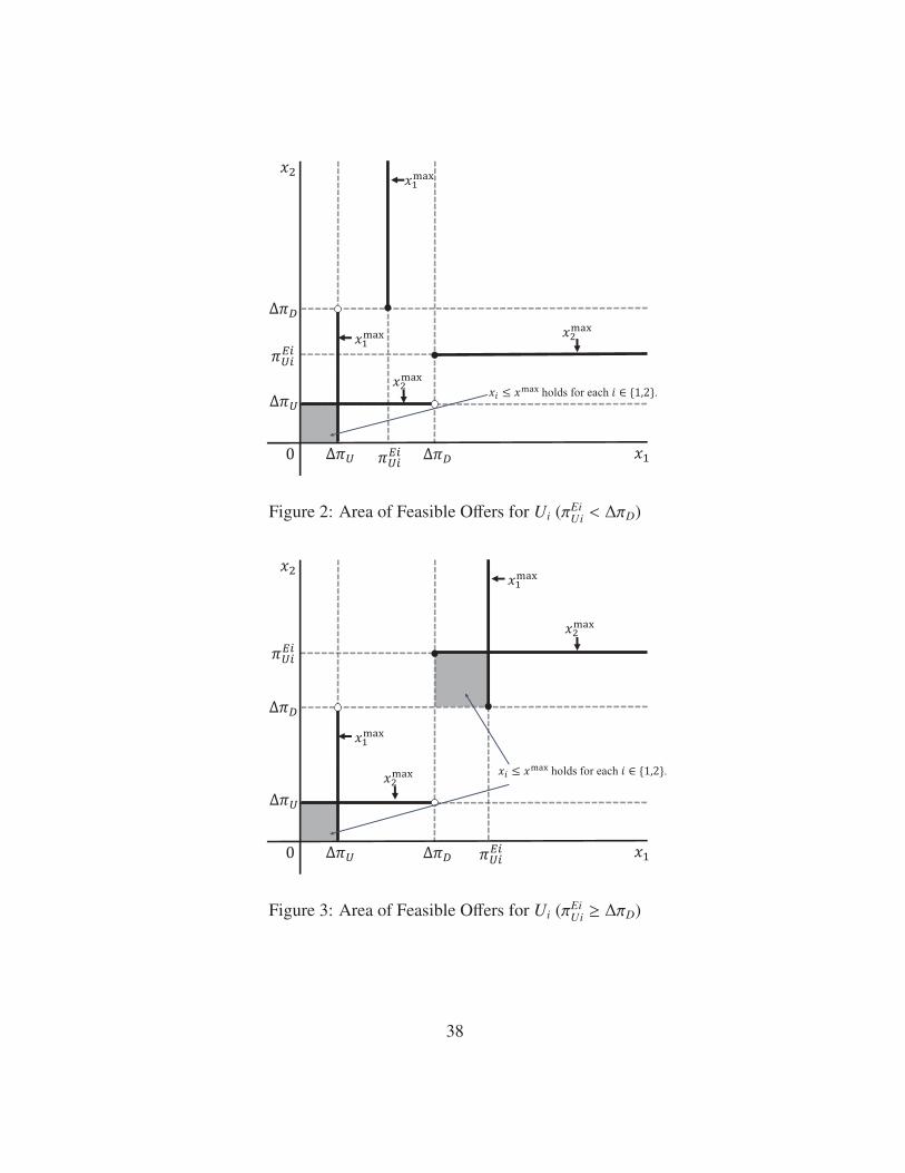
Figures 2 and 3 summarize the set of each manufacturer’s feasible offer (x1, x2) that sat-

isfies xi ∈ [0, xmax] for each i ∈ {1, 2}. Each manufacturer’s offer is feasible in the shadowed

area of Figures 2 and 3, which can be a candidate for the set of exclusion offers in the exclu-

sion equilibrium (x∗∗1 , x∗∗2 ); in other words, other areas cannot be the exclusion equilibrium.

Depending on the magnitude relationship between πEiUi

and ∆πD, we have two cases. First,

if πEiUi< ∆πD, summarized in Figure 2, each manufacturer’s exclusive offer is feasible in only

one region because D’s rejection profit is considerably high and each manufacturer cannot

compensate D profitably when its rival makes the higher offer. Second, if πEiUi≥ ∆πD, sum-

marized in Figure 3, each manufacturer’s exclusive offer is feasible in two regions. Because

D’s rejection profit is not too high in this case, Ui can profitably offer xi(≥ ∆πD) when U j

makes the high offer x j ≥ (∆πD).

[Figures 2 and 3 about here]

To explore the existence of an exclusion equilibrium, we now combine the results in

Figures 1, 2, and 3. Figures 4 and 5 combine these figures and D’s decision in the shadowed

12

areas in Figures 2 and 3. Figure 4 implies that exclusion never occurs if πEiUi< ∆πD. In this

case, there exist only non-exclusion equilibria in which each manufacturer offers xi ∈ [0,∆πD)

and D rejects both offers. By contrast, Figure 5 shows that an exclusion equilibrium exists if

πEiUi≥ ∆πD. The candidate for the equilibrium offer is the area in which (x1, x2) ∈ [∆πD, π

EiUi

]2

holds. Obviously, xi > x j ≥ ∆πD and xi = x j < πEiUi

cannot be an equilibrium because at least

one of the manufacturers has an incentive to deviate. There exists the exclusion equilibrium

in which each manufacturer offers x∗∗i= πEi

Uiand D accepts one of the offers. Note that even

when πEiUi≥ ∆πD, there also exists the non-exclusion equilibria in which each manufacturer

offers xi ∈ [0,∆πD) and D rejects both offers.

[Figures 4 and 5 about here]

We finally consider the existence of an exclusion equilibrium. From the above discussion,

we need to check whether πEiUi≥ ∆πD holds. By substituting Equations (2) and (3), we obtain

πEiUi − ∆πD = (1 − 2β)(2Πd − Πm) ≥ 0,

if and only if β ∈ (0, 1/2], which implies that an exclusion equilibrium exists for the weak

bargaining power of D.

Proposition 2. Suppose that both manufacturers make exclusive offers in Stage 1 and adopt

two-part tariffs in Stage 2. If D has strong bargaining power (β > 1/2), exclusion cannot be

an equilibrium outcome. By contrast, if D has weak bargaining power (β ≤ 1/2), there exist

both an exclusion equilibrium and non-exclusion equilibria.

Proposition 2 shows that under exclusive-offer competition, an exclusion equilibrium ex-

ists depending on the bargaining power of D over manufacturers. For the weak bargaining

power of D, D earns a lower profit when it rejects both exclusive offers in Stage 1. Therefore,

each manufacturer can compensate D profitably. Moreover, the existence of an exclusion

equilibrium does not depend on the degree of product substitution γ under non-linear whole-

sale pricing. Note that the result here highly depends on the assumption that manufacturers’

13

costs are symmetric. In the following subsection, we explore the case of an asymmetric cost

structure and show that the exclusion equilibrium is more likely to be observed for lower γ.

Note that Proposition 2 shows that exclusion is not a unique equilibrium outcome. By

comparing the two types of equilibria, the manufacturers strictly prefer the non-exclusion

equilibria to the exclusion equilibrium. Seemingly, the cola wars capture the exclusion equi-

librium because both Coca-Cola and PepsiCo pay a large monetary transfer. The likelihood

of exclusion here may depend on the market history. If a president of one upstream firm has

a managerial incentive to maximize market share rather than profit, exclusion is more likely

to occur. Once exclusion occurs, it is more likely to be observed continuously—even when

the managerial incentive changes. In addition, D has a strong incentive to yield the exclusion

outcome. Because Condition (4) holds with strict inequality under the exclusion equilibrium,

D prefers the exclusion equilibrium to the non-exclusion equilibrium. Hence, D may try to

do something to yield the exclusion outcome.

3.4 Cost asymmetry

This subsection briefly discusses the effect of cost asymmetry on the existence of an exclusion

equilibrium. Thus far, we have assumed that each manufacturer operates at the same marginal

cost c ≥ 0. We now extend the model to the case in which manufacturers operate at different

marginal costs. Without loss of generality, we assume that the marginal cost of U1 is lower

than that of U2, namely 0 ≤ c1 < c2. We define pmi and pdi as follows:

pmi ≡ arg maxpi

(pi − ci)Q(pi),

(pdi, pd j) ≡ arg maxpi,p j

(pi − ci)Q(pi, p j) + (p j − c j)Q(p j, pi).

We define Πmi and Πdi as the net profit of Ui’s vertical chain under upstream monopoly and

upstream duopoly:

Πmi ≡ (pmi − ci)Q(pmi), Πdi ≡ (pdi − ci)Q(pdi, pd j).

14

Since our focus is the existence of anticompetitive exclusive dealing, we only consider the

case where the upstream market becomes a duopoly in the absence of exclusive dealing,

namely Πdi > 0 for each i ∈ {1, 2}. For the sake of notational convenience, we define

∆Πi ≡ Πdi + Πd j − Πm j,

which can be interpreted as the level of increment in the industry profit when Ui’s product is

also launched in the upstream market monopolized by U j. As in Assumption 1, we assume

the following relationships:

Assumption 2. Πmi and Πdi have the following properties:

1. Trading with U1 leads to higher profits than that with U2;

Πm1 > Πm2, Πd1 > Πd2. (8)

2. For each i ∈ {1, 2} and γ ∈ (0, 1),

Πd1 + Πd2 > Πmi > Πdi, (9)

where ∂Πmi/∂γ = 0, ∂Πdi/∂γ < 0, Πdi → Πmi as γ → 0, and Πd2 → 0 and Πd1 → Πm1

for sufficiently high γ.

3. ∆Π1 is decreasing in c1 but ∆Π2 is increasing in c1:

∂∆Π1

∂c1

< 0,∂∆Π2

∂c1

> 0. (10)

Note that Conditions (8) and (9) imply that

∆Π1 > ∆Π2 > 0. (11)

By using the above definitions, we can derive the equilibrium profits under asymmetric

costs. As in Section 3.1, the negotiation between Di and Ui leads to marginal cost pricing in

15

all cases. Under generalized Nash bargaining, the firms’ equilibrium profits under exclusive

dealing, excluding the fixed compensation xi, are

πEiUi = (1 − β)Πmi, π

EiU j = 0, πEi

D = βΠmi. (12)

By contrast, the firms’ equilibrium profits under non-exclusive dealing are

πRUi = (1 − β)∆Πi, π

RD = (1 − β)(Πmi − Πdi + Πm j − Πd j) + β(Πdi + Πd j). (13)

From Condition (10), we have ∂πRU1/∂c1 < 0 but ∂πR

U2/∂c1 > 0, which is observed in the

linear demand model.17

We now consider the existence of an exclusion equilibrium. We first explore the case in

which only Ui can make an exclusive offer. By substituting Equations (12) and (13), we find

that under Condition (9)

πEiUi + π

EiD − (πR

Ui + πRD) = −β∆Π j < 0,

which implies that exclusion never occurs.

Proposition 3. Suppose both manufacturers adopt two-part tariffs. If U j is a potential entrant

and only Ui can make an exclusive offer, Ui cannot exclude U j through exclusive contracts

even under asymmetric costs.

Proposition 3 implies that U1 cannot deter the entry of U2 as long as entry increases the

industry profit. Therefore, the result confirms the robustness of the Chicago School argument

in the case where the incumbent manufacturer cannot deter the entry of a potential entrant

manufacturer, which is even less efficient.

We next consider the case in which both manufacturers make exclusive offers. Note that

the exclusion equilibrium exists if and only if πEiUi+ πEi

D≥ πR

D holds for each i ∈ {1, 2}. By

substituting Equations (12) and (13), we have πEiUi+ πEi

D− πR

D ≥ 0 if and only if

β ≤ βi ≡∆Πi

∆Πi + ∆Π j

(14)

17 See Appendix C, which introduces the results under the linear demand model.

16

for each i ∈ {1, 2}. From Conditions (11) and (14), βi have the following relationships:

0 < β2 <1

2< β1 < 1, (15)

where β1 → 1 and β2 → 0 as ∆Π2 → 0. Condition (15) shows that β1 > β2 always holds;

thus, the exclusion equilibrium exists if and only if β ≤ β2. Because β2 < 1/2 always holds,

cost asymmetry reduces the possibility of the exclusion equilibrium. More precisely, by

differentiating βi with respect to c1, we have

∂βi

∂c1

=1

(∆Πi + ∆Π j)2

(

∂∆Πi

∂c1

∆Π j −∂∆Π j

∂c1

∆Πi

)

.

Under Condition (10), we have ∂β1/∂c1 < 0 and ∂β2/∂c1 > 0. Therefore, as U1 becomes

more efficient, β2 decreases; in other words, the exclusion equilibrium is less likely to exist.

The following proposition summarizes the results provided above.

Proposition 4. Suppose that both manufacturers make exclusive offers in Stage 1 and adopt

two-part tariffs in Stage 2. As the degree of cost asymmetry increases, exclusion is less likely

to be an equilibrium outcome.

The result in Proposition 4 implies that the exclusion mechanism in this study is more

likely to work well when each manufacturer has a similar cost structure. When U1’s efficiency

increases, the industry profit under duopoly Πd1 + Πd2 increases, which allows D to earn

higher profits under upstream duopoly because ∂πRD/∂c1 = −(1−β)∂∆Π2/∂c1 +β(∂Πd1/∂c1 +

∂Πd2/∂c2) < 0. By contrast, the increase in U1’s efficiency does not affect U2’s monopoly

profit under exclusive dealing; hence, U2 has difficulty in compensating D. Therefore, the

possibility of exclusion becomes lower under cost asymmetry.

Finally, we explore the relationship between the existence of an exclusion equilibrium

and the degree of product substitution γ. By differentiating βi with respect to γ, we have

∂βi

∂γ=Πm j − Πmi

(∆Πi + ∆Π j)2

(

∂Πdi

∂γ+∂Πd j

∂γ

)

> 0 if and only if Πmi > Πm j.

From Condition (8), we have ∂β1/∂γ > 0 and ∂β2/∂γ < 0, which lead to the following

proposition.

17

Proposition 5. Suppose that both manufacturers make exclusive offers in Stage 1 and adopt

two-part tariffs in Stage 2. Under cost asymmetry, the exclusion equilibrium is more likely to

be observed for the cases in which the manufacturers produce highly differentiated products.

The result in Proposition 5 implies that under cost asymmetry, the existence of an exclu-

sion equilibrium is determined by the degree of product substitution γ; in other words, the

result in Proposition 2 highly depends on the symmetric cost structure. The result here is ex-

plained by the property of bargaining when D rejects both exclusive offers. By differentiating

πRD

with respect to γ, we have

∂πRD

∂γ= (2β − 1)

(

∂Πd1

∂γ+∂Πd2

∂γ

)

> 0 for β < 1/2,

which implies that as the manufacturers produce less differentiated products, D earns high

profits under upstream duopoly for the weak bargaining power of D. The degree of product

substitution affects D’s profit under upstream duopoly in two ways. First, as γ increases, the

industry profit Πdi + Πd j directly decreases, which has the negative effect of decreasing πRD

.

Second, because Ui’s additional contribution decreases, it earns lower profits πRUi= FR

i, which

indirectly increases D’s outside option profit under the bargaining with U j, z j = Πmi−FRi. This

indirect effect increases πRD

and becomes dominant for lower β because the strong bargaining

power of Ui decreases FRi

largely. Under this relationship, as the manufacturers produce

more differentiated products when the downstream firm has weak bargaining power, U2 can

compensate D more easily; thus, the exclusion equilibrium is more likely to be observed.18

4 Discussion

This section briefly discusses the wholesale pricing and real-world examples of exclusive-

offer competition. Section 4.1 extends the analysis to the case of linear wholesale pricing.

18 When the downstream firm and each manufacturer have the same bargaining power (β = 1/2), we have

∂πRD/∂γ = 0; thus, the degree of product substitution does not affect D’s profit under upstream duopoly. Since

the threshold value of D’s bargaining power under symmetric costs is 1/2, the likelihood of exclusion under

symmetric costs does not depend on product substitution.

18

Section 4.2 introduces some examples of exclusive-offer competition.

4.1 Linear wholesale pricing

This subsection explores the existence of anticompetitive exclusive dealing under linear whole-

sale pricing by assuming standard linear demand with a representative consumer, in which

demand for Ui’s product is provided by

Q(pi, p j) =

a − pi

bif 0 < pi ≤

−a(1 − γ) + p j

γ,

a(1 − γ) − pi + γp j

b(1 − γ2)if−a(1 − γ) + p j

γ< pi < a(1 − γ) + γp j,

0 if pi ≥ a(1 − γ) + γp j,

(16)

where i, j ∈ {1, 2} and i , j. As in the previous section, we assume that the industry profit

allocation after Stage 1 is given by the Nash bargaining solution.

We first explore the existence of an exclusion equilibrium when only Ui can make an

exclusive offer. Like the case of two-part tariffs, exclusion never occurs.

Proposition 6. Suppose both manufacturers offer linear wholesale prices. If U j is a potential

entrant and only Ui can make an exclusive offer, Ui cannot exclude U j through exclusive

contracts for any pair of bargaining power allocation and the degree of product substitution.

Proof. See Appendix A.1. �

Proposition 6 implies that in the absence of exclusive-offer competition, anticompetitive

exclusive dealing cannot occur, which can be explained by the logic underlying the Chicago

School argument.

We next investigate the existence of an exclusion equilibrium when both manufacturers

can make exclusive offers. In this case, an exclusion equilibrium exists under some condi-

tions.

Proposition 7. Suppose that both manufacturers make exclusive offers in Stage 1 and linear

wholesale prices are determined through Nash bargaining in Stage 2. When the products

19

are less differentiated (γ > γ ≃ 0.77393), exclusion cannot be an equilibrium outcome. By

contrast, when those are sufficiently differentiated (γ ≤ γ), there exist both an exclusion

equilibrium and non-exclusion equilibria for a sufficiently weak bargaining power of D (β ≤

β(γ)), where

β(γ) ≡4φ2 + 2γ(1 + γ)(5γ − 4)φ + 4γ2(1 + γ)(γ3 + 3γ2 + 3γ − 5)

6γ2(1 + γ)φ,

and

φ ≡[

γ3(1 + γ)2(γ4 + 4γ3 + 6γ2 − 32γ + 19)

+3

√

6γ6(1 + γ)2(1 − γ2)(

γ5 + 5γ4 + 10γ3 + 5γ3 − 12γ2 − 11γ + 9)

]

13

.

Proof. See Appendix A.2. �

Note that β(γ) has a single peaked property with β(γ) → 1/3 as γ → 0, β(γ) → 0 as γ → γ,

and the maximized value β(γ∗) ≃ 0.413049 at γ∗ ≃ 0.469146.

[Figure 6 about here]

Figure 6 summarizes Proposition 7. The notable result in Proposition 7 is that linear

wholesale pricing leads to the low possibility of the anticompetitive exclusion equilibrium;

exclusion never occurs for the intermediate level of D’s bargaining power or for less differ-

entiated manufacturers’ products.

The major difference between two types of pricing is the existence of double marginaliza-

tion problems, which arise not only under exclusive dealing but also under upstream duopoly.

These two double marginalization problems reduce the possibility of exclusive outcomes in

the following ways. Under exclusive dealing, the contracting party cannot achieve the joint

profit maximization due to the double marginalization problem. Because upstream duopoly

can mitigate such a problem, manufacturers have difficulty in compensating D for the inter-

mediate level of D’s bargaining power. Moreover, the mitigation effect of upstream duopoly

20

depends on the degree of product substitution γ. When the manufacturers produce almost ho-

mogeneous products, the double marginalization problem under upstream duopoly is not too

serious, which allows D to earn large rejection profits πRD. Hence, the exclusion equilibrium

does not exist when the products are less differentiated.

4.2 Cola wars in the real world

In this subsection, we provide examples of exclusive-offer competition in the soft drinks in-

dustry. For instance, cola wars have continued for decades between Coca-Cola and PepsiCo,

with each aiming to be the exclusive beverage provider to fast food restaurants.19 Through

exclusive-offer competition, some customers shift from one manufacturer to the other. For

example, Arby’s Restaurant Group Inc. decided to switch from PepsiCo to Coca-Cola start-

ing from early 2018 after more than a decade-long contract with PepsiCo.20 Subway had had

a partnership with PepsiCo as its primary beverage provider since 1988; however, in 2003, it

decided to make a transition to Coca-Cola in its worldwide restaurants.21 From 2015, Pep-

siCo Canada started to serve Subway Canada as its exclusive beverage and snack provider.22

Another example of the exclusive-offer competition between these two giant suppliers can

be observed on university campuses, as noted in Introduction.23 The cola wars forming on

university campuses are widespread in the United States and contain some of the key features

in our analysis. First, exclusive-offer competition involves a large monetary transfer in return

for a long-term monopoly position; for example, in 1998, The University of Maryland at Col-

19 Cola wars have also been observed in the relationship between the cola providers and cinemas. See “Coca-

Cola Lures Regal Cinemas From Rival Pepsi in Latest Steal” The Wall Street Journal, April 9, 2002 (link).

20 See “Coca-Cola Wins Arby’s Away From PepsiCo in Latest Showdown” Bloomberg, August 18, 2017

(link).

21 See “Coke Wins a 10-Year Contract From Subway, Ousting PepsiCo” The Wall Street Journal, November

28, 2003 (link).

22 See the second paragraph from the bottom in “Coca-Cola Wins Arby’s Away From PepsiCo in Latest

Showdown”

23 Regarding universities’ switch between Coca-Cola and PepsiCo, see “Coke vs. Pepsi: University Chooses

Side In Cola Wars” Montclair Patch, July 12, 2016 (link).

21

lege Park signed a 15-year exclusive contract with PepsiCo worth $57.5 million.24 Second,

universities receive not only an annual royalty fee but also a commission fee from the retail

sale of some products. The commission rates, which could be correlated to β in our analysis,

vary across universities. In the case of Ohio State University and Rutgers University, they

range from about 20 percent to over 50 percent of the retail sale of drinks and snacks.25 Fi-

nally, universities are usually local monopolists; hence, exclusive-offer competition is more

likely to play an essential role in exclusion. Although the objective of universities may not

be to maximize their profits, our results remain valid even when universities are consumer-

surplus maximizers.26 Therefore, we think that our analysis fits the cola wars on university

campuses well.

Although the above examples are not antitrust cases, the cola wars sometimes lead to

antitrust cases. For example, in 1998, PepsiCo filed an antitrust lawsuit against Coca-Cola,

alleging that Coca-Cola did not allow food-service distributers who already distribute Coke

to distribute Pepsi.27 The notable point here is that Coca-Cola was stronger in the food-

service distribution sector of the soft drinks market than in the overall market; the food-

service distributors’ share of Coca-Cola was 65 percent and that of PepsiCo was 22 percent,

while in the overall soft drinks market Coca-Cola had a 43.9 percent share and PepsiCo had

a 30.9 percent share. Therefore, if one side has an extremely higher market share in one area

because of exclusive dealing, it will be more likely to take the cola wars to court.

24 See “Thirsting For Cash, Colleges Take Sides In Corporate Cola Wars” The Washington Post, December

23, 1997 (link).

25 For the case of Ohio State University, see “Refreshing or restricting? Ohio States $32M deal with Coca-

Cola brings up questions of transparency” The Lantern, December 19, 2013 (link). In addition, for the case of

Rutgers University, see “As of May 2005, Rutgers University no longer has a contract with Coca-Cola” Rutgers

University, May, 2005 (link).

26 The results are available upon request.

27 See “Taking The ’Cola Wars’ Into Court” The Washington Post, May 31, 1998 (link).

22

5 Conclusion

This study has explored the existence of anticompetitive exclusive dealing when all upstream

firms can make exclusive offers. Most previous studies consider anticompetitive exclusive

dealing to deter a potential entrant, which cannot make an exclusive offer. However, in the

real-world situation, existing firms are often excluded. Therefore, we need to consider how

the existence of exclusive-offer competition affects the possibility of exclusion to apply the

model to these cases.

We show that a seemingly small difference in the setting turns out to be crucial. In contrast

to the case where one of the upstream firms is a potential entrant, the existence of exclusive-

offer competition eliminates upstream firms’ opportunity to earn positive profits when they

fail to exclude the rival upstream firm. We point out that this induces upstream firms to

make higher exclusive offers and show that when the downstream firm has weak bargaining

power, anticompetitive exclusive dealing can be an equilibrium outcome in the two-part tariff

setting of the general demand function and Nash bargaining. Moreover, this result holds in

various settings and thus the exclusion outcome identified in this study can be widely applied

to diverse real-world vertical relationships.

The finding here provides new implications for antitrust agencies; anticompetitive exclu-

sive dealing is more likely to be observed when upstream firms are existing firms. In addition,

because the downstream firm has a strong incentive to engage in anticompetitive exclusive

dealing, it is more likely to lead the negotiation of anticompetitive exclusive dealing when

upstream firms are existing firms.

Despite these contributions, there remain several outstanding issues requiring future re-

search. First, there is a concern about upstream firms’ behavior to achieve a market environ-

ment where an exclusion equilibrium does not exist. Although we assume that the level of

product substitution or bargaining power is exogenously given, upstream firms could control

these parameters. Second, there is a concern about this study’s relationship with other studies

of anticompetitive exclusive dealing. We predict that if we add exclusive-offer competition

23

into previous studies, exclusion becomes less costly. We hope that this study will assist future

researchers in addressing these issues.

24

A Proofs of the results

A.1 Proof of Proposition 6

Before proceeding to the proof, we derive firms’ equilibrium profits in the subgame after D’s

decision in Stage 1.

We first explore the case in which Ui’s exclusive offer is accepted in Stage 1. Under

exclusive dealing, the final consumer’s demand for Ui’s product becomes Q(pi) = (a − pi)/b.

We solve the game by using backward induction. In Stage 3, given wi determined in Stage

2, D optimally chooses the price of Ui’s product, namely p∗(wi) ≡ arg maxpi(pi − wi)Q(pi) =

(a + wi)/2. The optimal production level of Ui’s product supplied by D given wi becomes

Q∗(wi) ≡ Q(p∗(wi)) = (a−wi)/2b. In Stage 2, Ui and D negotiate and make a contract for the

linear wholesale price wEii

. By defining D’s profit given wi asΠ∗(wi) ≡ (p∗(wi)−wi)Q∗(wi), the

bargaining problem between D and Ui is described by the payoff pairs (Π∗(wi), (wi−c)Q∗(wi))

and the disagreement point (0, 0). The solution is given by

wEii = arg max

wi

β logΠ∗(wi) + (1 − β) log[(wi − c)Q∗(wi)].

The maximization problem leads to

wEii =

a + c − β(a − c)

2.

The firms’ equilibrium profits, excluding the fixed compensation xi, are

πEiUi =

(1 − β2)(a − c)2

8b, πEi

U j = 0, πEiD =

(1 + β)2(a − c)2

16b. (17)

We next explore the case in which D rejects both exclusive offers in Stage 1. In Stage 3,

given the wholesale prices wi and w j determined in Stage 2, D optimally chooses the prices

of each manufacturer’s product (p∗(wi,w j), p∗(w j,wi)), where

(p∗(wi,w j), p∗(w j,wi)) ≡ arg max

pi,p j

(pi − wi)Q(pi, p j) + (p j − w j)Q(p j, pi),

25

where i, j ∈ {1, 2} and i , j. The production level of each final product supplied by D given

wi and w j is given by

Q∗(wi,w j) ≡ Q(p∗(wi,w j), p∗(w j,wi)) =

a − wi − γ(a − w j)

2(1 − γ2)b.

In Stage 2, U1, U2, and D make contract(s) for the linear wholesale prices wR1 and wR

2 . By

defining D’s profit from selling Ui’s product given (wi,w j) as Π∗(wi,w j) ≡ (p∗(wi,w j) −

wi)Q∗(wi,w j), the bargaining problem between D and Ui is described by the payoff pairs

(Π∗(wRi ,w

Rj )+Π

∗(wRj ,w

Ri ), (wR

i − c)Q∗(wRi ,w

Rj )) and the disagreement point (Π∗(wR

j ), 0), where

Π∗(wRj ) is D’s profit when it sells only U j’s product given the linear wholesale price wR

j . The

solution is given by

wRi = arg max

wi

β log[Π∗(wi,w j) + Π∗(w j,wi) − Π

∗(w j)] + (1 − β) log[(wi − c)Q∗(wi,w j)].

The maximization problem leads to

wRi =

a(1 − γ) + c − β(a(1 − γ) − c)

2 − γ(1 − β),

for each i ∈ {1, 2}. The resulting profits of the firms are given as

πRUi =

(1 − β2)(1 − γ)(a − c)2

2b(1 + γ)(2 − γ(1 − β))2, πR

D =(1 + β)2(a − c)2

2b(1 + γ)(2 − γ(1 − β))2. (18)

We now consider the existence of an exclusion equilibrium. We show that Condition (6)

never holds; in other words, by substituting Equations (17) and (18), we have

∆πU − ∆πD = −(a − c)2(1 + β)(8 − (1 + γ)(2 − γ(1 − β))(3 − β))

16b(1 + γ)(2 − γ(1 − β))< 0, (19)

for all (β, γ) ∈ (0, 1)2. Let η(β, γ) ≡ −8 + (1 + γ)(2 − γ(1 − β))(3 − β). Note that η(β, γ) < 0 if

and only if Condition (19) holds. By differentiating η(β, γ) with respect to β and γ, we have

ηβ(β, γ) R 0⇔ β ⋚ K(γ) ≡−1 + 2γ

γ,

ηγ(β, γ) R 0⇔ β R L(γ) ≡−1 + 2γ

1 + 2γ.

26

Note that for γ ∈ (1/2, 1], K′(γ) > L′(γ) > 0 and K(γ) > L(γ) > 0 and that K(1/2) =

L(1/2) = 0 and K(1) = 1 and L(1) = 1/3. Figure 7 summarizes the properties of ηβ(β, γ)

and ηγ(β, γ). There are six regions in (β, γ) ∈ [0, 1]2 such that (i) ηβ(β, γ) = ηγ(β, γ) = 0, (ii)

ηβ(β, γ) < 0, ηγ(β, γ) > 0, (iii) ηβ(β, γ) = 0, ηγ(β, γ) > 0, (iv) ηβ(β, γ) > 0, ηγ(β, γ) > 0, (v)

ηβ(β, γ) > 0, ηγ(β, γ) = 0, and (vi) ηβ(β, γ) > 0, ηγ(β, γ) < 0. The arrows in Figure 7 indicate

the direction of the increase in η(β, γ) for each region. From Figure 7, for (β, γ) = (0, 1/2),

η(β, γ) takes the locally maximized value in region (i), where we have η(β, γ) = −5/4 < 0.

More importantly, Figure 7 shows that η(β, γ) is globally maximized in the domain (β, γ) ∈

[0, 1]2 when (β, γ) = (1, 1), where we have η(1, 1) = 0. Therefore, η(β, γ) < 0 for all

(β, γ) ∈ (0, 1)2.

Q.E.D.

A.2 Proof of Proposition 7

We check whether πEiUi≥ ∆πD holds. By substituting Equations (17) and (18), we obtain

πEiUi− ∆πD ≥ 0 if and only if γ ≤ γ and β ≤ β(γ) < 1/2.

Q.E.D.

B Results under linear demand and symmetric costs

This appendix introduces the analysis of the model in Section 3.1–3.3 under the linear de-

mand function (16). Under the linear demand function, we have

Πm =(a − c)2

4b, Πd =

(a − c)2

(1 + γ)b. (20)

Then, the firms’ equilibrium profits under exclusive dealing, excluding the fixed compensa-

tion xi, are

πEiUi =

(1 − β)(a − c)2

4b, πEi

U j = 0, πEiD =β(a − c)2

4b. (21)

27

The profits of firms under no exclusive dealing are given as

πRUi =

(1 − β)(1 − γ)(a − c)2

4b(1 + γ), πR

D =(β(1 − γ) + γ)(a − c)2

2b(1 + γ). (22)

We now explore the existence of an exclusion equilibrium. For the case in which only

Ui can make an exclusive offer, we check whether Condition (6) holds. By substituting

Equations (21) and (22), we have

∆πU − ∆πD = −β(1 − γ)(a − c)2

4b(1 + γ)< 0, (23)

for all γ ∈ [0, 1) and β ∈ (0, 1); as with linear wholesale pricing, exclusion never occurs. This

result is consistent with Proposition 1.

By contrast, for the existence of an exclusion equilibrium when both manufacturers can

make exclusive offers, we check whether πEiUi≥ ∆πD holds. By substituting Equations (21)

and (22), we have

πEiUi − ∆πD =

(1 − 2β)(1 − γ)(a − c)2

4b(1 + γ)≥ 0, (24)

for β ∈ (0, 1/2]. Therefore, an exclusion equilibrium exists if β ≤ 1/2, which is consistent

with Proposition 2.

C Results under linear demand and asymmetric costs

This appendix introduces the analysis of the model in Section 3.4 under the linear demand

function (16). We measure U1’s cost advantage by θ, where c2 = θpm1 + (1 − θ)c1 and

pm1 = (a + c1)/2. θ = 0 implies that U1 has no cost advantage. As θ increases, U1 becomes

efficient. We assume the following relationship:

0 < θ < min{2(1 − γ), 1}. (25)

If Condition (25) holds, the upstream market becomes a duopoly if the exclusive offer is

rejected. When D accepts U1’s exclusive offer, the firms’ equilibrium profits, excluding the

fixed compensation x1, are

πE1U1 =

(1 − β)(a − c2)2

(2 − θ)2b, πE1

U2 = 0, πE1D =

β(a − c2)2

(2 − θ)2b. (26)

28

Likewise, when D accepts U2’s exclusive offer, the firms’ equilibrium profits, excluding the

fixed compensation x2, are

πE2U2 =

(1 − β)(a − c2)2

4b, πE2

U1 = 0, πE2D =

β(a − c2)2

4b. (27)

By contrast, when D rejects both exclusive offers, the firms’ equilibrium profits are

πRD =

(θ2 + 4(1 − γ)(2 − θ) − (1 − β)((2(1 − γ) + θγ)2 + (2(1 − γ) − θ)2))(a − c2)2

4b(1 − γ2)(2 − θ)2,

πRU1 =

(1 − β)(2(1 − γ) + θγ)2(a − c2)2

4b(1 − γ2)(2 − θ)2, πR

U2 =(1 − β)(2(1 − γ) + θ)2(a − c2)2

4b(1 − γ2)(2 − θ)2.

(28)

We now consider the existence of an exclusion equilibrium when both manufacturers

make exclusive offers. By substituting (26), (27), and (28), πEiUi+ πEi

D− πR

D ≥ 0 if and only if

β ≤ βi(γ, θ), where

β1(γ, θ) ≡(2(1 − γ) + θγ)2

4(1 − γ)2(2 − θ) + θ2(1 + γ2), β2(γ, θ) ≡

(2(1 − γ) − θ)2

4(1 − γ)2(2 − θ) + θ2(1 + γ2).

The following lemma summarizes the properties of βi(γ, θ).

Proposition C.1. βi(γ, θ) has the following properties:

1. 0 < β2 < 1/2 < β1 < 1.

2. ∂β1/∂γ > 0 and ∂β2/∂γ < 0.

3. ∂β1/∂θ > 0 and ∂β2/∂θ < 0.

4. As γ→ (2 − θ)/2, β1 → 1 and β2 → 0.

5. As θ→ 0, β1 → 1/2 and β2 → 1/2.

Proof. We examine the first property. Note that β2 > 0 is obvious. Then, we have

β1 −1

2=

1

2− β2 =

(θ(4 − θ)(1 − γ))2

2(4(1 − γ)2(2 − θ) + θ2(1 + γ2))> 0,

29

1 − β1 =(2(1 − γ) − θ)2

4(1 − γ)2(2 − θ) + θ2(1 + γ2)> 0.

Therefore, the first property holds. The second and third properties can be derived by the

following results; under Condition (25),

∂β1

∂γ=

2θ(4 − θ)(2(1 − γ) + θγ)(2(1 − γ) − θ)

4(1 − γ)2(2 − θ) + θ2(1 + γ2)> 0,

∂β2

∂γ= −

2θ(4 − θ)(2(1 − γ) + θγ)(2(1 − γ) − θ)

4(1 − γ)2(2 − θ) + θ2(1 + γ2)< 0,

∂β1

∂θ=

4(1 − γ2)(2(1 − γ) + θγ)(2(1 − γ) − θ)

4(1 − γ)2(2 − θ) + θ2(1 + γ2)> 0,

∂β2

∂γ= −

4(1 − γ2)(2(1 − γ) + θγ)(2(1 − γ) − θ)

4(1 − γ)2(2 − θ) + θ2(1 + γ2)< 0.

The fourth and fifth properties are obtained by substituting γ = (2 − θ)/2 and θ = 0 into

βi(γ, θ), which is continuous in θ and γ. �

D Exclusive supply contracts when downstream firms com-

pete in quantity

This appendix introduces another case where exclusive-offer competition plays an essential

role in exclusive dealing. The upstream market is composed of an upstream monopolist U,

whose marginal cost is c ≥ 0. The downstream market is composed of two downstream firms

that produce homogeneous products. Each downstream firm produces one unit of the final

product by using one unit of input produced by U. For simplicity, we assume that the cost

of transformation is zero for each Di; given the input price w, the per unit production cost

of Di is given by cDi = wi, where i ∈ {1, 2}. D1 and D2 compete in quantity. Let Qi be the

production level of Di. We assume that inverse demand for the final product P(Q) is given by

a simple linear function:

P(Q) = a − bQ,

where Q ≡ Q1 + Q2 is the output of the final product, a > c, and b > 0.

30

The model in this appendix contains three stages. In Stage 1, D1 and D2 make exclusive

supply offers to U with fixed compensation yi ≥ 0, where i ∈ {1, 2}. U can reject both offers or

accept one of the offers. As defined in Section 2, let ω ∈ {R, E1, E2} be U’s decision in Stage

1. If U is indifferent between these two exclusive offers and acceptance is more profitable, it

accepts one of the offers with probability 1/2. In Stage 2, U offers linear wholesale price w

to active downstream firms. The equilibrium wholesale price offered by U is denoted by wω.

In Stage 3, active downstream firms order inputs and determine the production level of the

final product Qi. Di’s profit is denoted by πωDi

. Likewise, U’s profit is denoted by πωU

.

D.1 Equilibrium outcomes after Stage 1

We first explore the case in which Di’s exclusive supply offer is accepted by U in Stage 1.

In Stage 3, given w, Di optimally chooses the production level QEii

(w) ≡ arg maxQi(P(Qi) −

w)Qi = (a − w)/2b. Then, input demand for U becomes QEi(w) = QEii

(w) = (a − w)/2b. In

Stage 2, by anticipating these results, U optimally chooses input price wEi ≡ arg maxw(w −

c)Q(w) = (a + c)/2. The equilibrium production levels become QEi = QEii= (a − c)/4b and

QEij= 0, where i, j ∈ {1, 2} and i , j. The firms equilibrium profits, excluding the fixed

compensation yi, are

πEiDi =

(a − c)2

16b, πEi

D j = 0, πEiD =

(a − c)2

8. (29)

We next explore the case in which U rejects the exclusive supply offers in Stage 1. In

Stage 3, given w, Di competes in quantity. Standard Cournot competition leads to QRi (w) =

(a − w)/3b. Then, input demand for U becomes QR(w) = 2(a − c)/3b. In Stage 2, by

anticipating these results, U optimally chooses input price wR ≡ arg maxw(w − c)QR(w) =

(a + c)/2. The equilibrium production levels become QR1 = QR

2 = (a − c)/6b. The firms’

equilibrium profits are

πRDi =

(a − c)2

36b, πR

U =(a − c)2

6b. (30)

31

D.2 Benchmark analysis

As in Section 3.2, we assume that D2 is a potential entrant and only Di can make an exclusive

offer in Stage 1. For an exclusion equilibrium to exist, the equilibrium transfer y∗i

must satisfy

the following two conditions.

First, the exclusive contract must satisfy individual rationality for U:

y∗i ≥ ∆πcU , (31)

where ∆πcU≡ πR

U− πEi

U.

Second, it must satisfy individual rationality for Di:

y∗i ≤ ∆πcD, (32)

where ∆πcD≡ πEi

Di− πR

Di.

From the above conditions, it is evident that an exclusion equilibrium exists if and only if

inequalities (31) and (32) simultaneously hold. This is equivalent to the following condition:

∆πcD ≥ ∆π

cU . (33)

We now consider the game in Stage 1. By substituting Equations (29) and (30), we obtain

∆πcD − ∆π

cU =

(a − c)2

144b< 0, (34)

which implies that Condition (33) never holds. Therefore, the exclusion outcomes cannot be

observed.

Proposition D.1. Suppose that downstream firms D1 and D2 compete in quantity by purchas-

ing inputs from upstream monopolist U. If D2 is a potential entrant and only D1 can make an

exclusive offer, D1 cannot exclude D2 via exclusive contracts.

The result here coincides with that of Appendix B in Kitamura, Matsushima, and Sato

(2017b).28

28 More precisely, both models coincide for k = 1 in their model.

32

D.3 When exclusive-offer competition exists

Assume that both downstream firms make exclusive offers. As in Section 3.3, the upper

bound of Di’s exclusive offer ymaxi

depends on D j’s offer, where

ymaxi ≡

{

πEiDi

if y j ≥ ∆πcU

∆πD if y j < ∆πcU

and where πEiDi> ∆πD.

For y j < ∆πcU

, we have ymax = ∆πcD

. With this offer, Ui earns πEiDi+ ymax < πR

Ubecause

inequality (34) holds; hence, the individual rationality constraint for U does not hold. There-

fore, as in Section 3.3, the non-exclusion equilibrium always exists. For the existence of an

exclusion equilibrium, we check whether πEiDi≥ ∆πc

Uholds. By substituting Equations (29)

and (30), we obtain

πEiDi − ∆π

cU =

(a − c)2

48b> 0,

which implies that the exclusion outcomes can be observed.

Proposition D.2. Suppose that downstream firms D1 and D2 compete in quantity by purchas-

ing inputs from upstream monopolist U. When both downstream firms can make exclusive

offers, there exist both an exclusion equilibrium and a non-exclusion equilibrium. In the ex-

clusion equilibrium, both D1 and D2 offer y∗i = πEiDi> ∆πU and U earns all the industry

profits.

References

Abito, J.M., and Wright, J., 2008. Exclusive Dealing with Imperfect Downstream Competi-

tion. International Journal of Industrial Organization 26(1), 227–246.

Aghion, P., and Bolton, P., 1987. Contracts as a Barrier to Entry. American Economic Re-

view 77(3), 388–401.

Argenton, C., 2010. Exclusive Quality. Journal of Industrial Economics 58(3), 690–716.

33

Bernheim, B.D., and Whinston, M.D., 1998. Exclusive Dealing. Journal of Political Econ-

omy 106(1), 64–103.

Bork, R.H., 1978. The Antitrust Paradox: A Policy at War with Itself. New York: Basic

Books.

Calzolari, G., and Denicolo, V., 2013. Competition with Exclusive Contracts and Market-Share

Discounts. American Economic Review 103(6), 2384–2411.

Calzolari, G., and Denicolo, V., 2015. Exclusive Contracts and Market Dominance. Ameri-

can Economic Review 105(11), 3321–3351.

Choi, J.P., and Stefanadis, C., 2017. Sequential Innovation, Naked Exclusion, and Upfront

Lump-Sum Payments. Economic Theory.

DOI: 10.1007/s00199-017-1042-3

DeGraba, P., 2013. Naked Exclusion by an Input Supplier: Exclusive Contracting Loyalty

Discounts. International Journal of Industrial Organization 31(5), 516–526.

Farrell, J., 2005. Deconstructing Chicago on Exclusive Dealing. Antitrust Bulletin 50, 465–

480.

Fumagalli, C., and Motta, M., 2006. Exclusive Dealing and Entry, when Buyers Compete.

American Economic Review 96(3), 785–795.

Fumagalli, C., Motta, M., and Calcagno, C., 2018. Exclusionary Practices: The Economics

of Monopolisation and Abuse of Dominance. Cambridge: Cambridge University Press.

Fumagalli, C., Motta, M., and Persson, L., 2009. On the Anticompetitive Effect of Exclusive

Dealing when Entry by Merger Is Possible. Journal of Industrial Economics 57(4),

785–811.

Fumagalli, C., Motta, M., and Rønde, T., 2012. Exclusive Dealing: Investment Promotion may

Facilitate Inefficient Foreclosure. Journal of Industrial Economics 60(4), 599–608.

34

Gans, J.S., 2013. Intel and Blocking Practices. The Antitrust Revolution: Economics, Com-

petition, and Policy. 6th Edition, edited by J. Kwoka and L. White, New York: Oxford

University Press.

Gratz, L., and Reisinger, M., 2013. On the Competition Enhancing Effects of Exclusive Deal-

ing Contracts. International Journal of Industrial Organization 31(5), 429-437.

Kitamura, H., 2010. Exclusionary Vertical Contracts with Multiple Entrants. International

Journal of Industrial Organization 28(3), 213–219.

Kitamura, H., Matsushima, N., and Sato, M., 2017a. Exclusive Contracts and Bargaining Power.

Economics Letters 151, 1–3.

Kitamura, H., Matsushima, N., and Sato, M., 2017b. How Does Downstream Firms’ Efficiency

Affect Exclusive Supply Agreements? mimeo.

http://ssrn.com/abstract=2306922

Kitamura, H., Matsushima, N., and Sato, M., 2018. Exclusive Contracts with Complemen-

tary Input. International Journal of Industrial Organization 56, 145–167.

Motta, M., 2004. Competition Policy. Theory and Practice. Cambridge: Cambridge Univer-

sity Press.

Posner, R.A., 1976. Antitrust Law: An Economic Perspective. Chicago: University of Chicago

Press.

Rasmusen, E.B., Ramseyer, J.M., and Wiley Jr., J.S., 1991. Naked Exclusion. American Eco-

nomic Review 81(5), 1137–1145.

Segal, I.R., and Whinston, M.D., 2000. Naked Exclusion: Comment. American Economic

Review 90(1), 296–309.

Shen, B., 2014. Naked Exclusion by a Manufacturer without a First-Mover Advantage, mimeo.

35

Simpson, J., and Wickelgren, A.L., 2007. Naked Exclusion, Efficient Breach, and Downstream

Competition. American Economic Review 97(4), 1305–1320.

Whinston, M.D., 2006. Lectures on Antitrust Economics. Cambridge: MIT Press.

Wright, J., 2008. Naked Exclusion and the Anticompetitive Accommodation of Entry. Eco-

nomics Letters 98(1), 107–112.

Wright, J., 2009. Exclusive Dealing and Entry, when Buyers Compete: Comment. American

Economic Review 99(3), 1070–1081.

Yong, J.S., 1996. Excluding Capacity-Constrained Entrants Through Exclusive Dealing: The-

ory and an Application to Ocean Shipping. Journal of Industrial Economics 44(2),

115–129.

Yong, J.S., 1999. Exclusionary Vertical Contracts and Product Market Competition. Journal

of Business 72(3), 385-406.

36

with

probability 1/2)

Figure 1: Individual Rationality for D

37

holds for each .

Figure 2: Area of Feasible Offers for Ui (πEiUi< ∆πD)

holds for each .

Figure 3: Area of Feasible Offers for Ui (πEiUi≥ ∆πD)

38

Figure 4: Existence of an Exclusion Equilibrium for πEiUi< ∆πD

Exclusion Equilibrium

with

probability 1/2)

Figure 5: Existence of an Exclusion Equilibrium for πEiUi≥ ∆πD

39

0.0 0.1 0.2 0.3 0.4 0.5 0.6 0.7 0.8 0.9 1.00.0

0.1

0.2

0.3

0.4

0.5

Figure 6: Existence of an Exclusion Equilibrium under Linear wholesale pricing

0.0 0.1 0.2 0.3 0.4 0.5 0.6 0.7 0.8 0.9 1.00.0

0.1

0.2

0.3

0.4

0.5

0.6

0.7

0.8

0.9

1.0

Figure 7: Properties of ηβ(β, γ) and ηγ(β, γ)

40