Embed Size (px)
Citation preview
Naïve Bayes
William W. Cohen
Probability - what you need to really, really know
• Probabilities are cool• Random variables and events• The Axioms of Probability• Independence, binomials, multinomials• Conditional probabilities• Bayes Rule• MLE’s, smoothing, and MAPs• The joint distribution• Inference

COMPUTING WITH A JOINT PROBABILITY ESTIMATE
Get some data
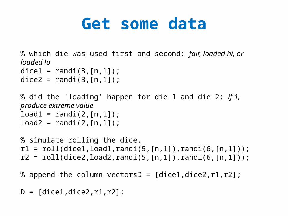
% which die was used first and second: fair, loaded hi, or loaded lodice1 = randi(3,[n,1]);dice2 = randi(3,[n,1]);
% did the 'loading' happen for die 1 and die 2: if 1, produce extreme valueload1 = randi(2,[n,1]);load2 = randi(2,[n,1]);
% simulate rolling the dice…r1 = roll(dice1,load1,randi(5,[n,1]),randi(6,[n,1]));r2 = roll(dice2,load2,randi(5,[n,1]),randi(6,[n,1]));
% append the column vectorsD = [dice1,dice2,r1,r2];
D = [dice1,dice2,r1,r2];
Get some data
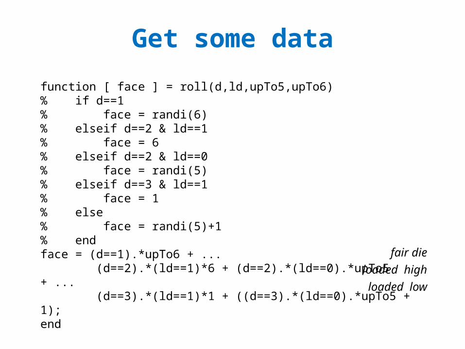
function [ face ] = roll(d,ld,upTo5,upTo6)% if d==1% face = randi(6)% elseif d==2 & ld==1% face = 6% elseif d==2 & ld==0% face = randi(5)% elseif d==3 & ld==1% face = 1% else % face = randi(5)+1% endface = (d==1).*upTo6 + ... (d==2).*(ld==1)*6 + (d==2).*(ld==0).*upTo5 + ... (d==3).*(ld==1)*1 + ((d==3).*(ld==0).*upTo5 + 1);end
fair die
loaded high
loaded low
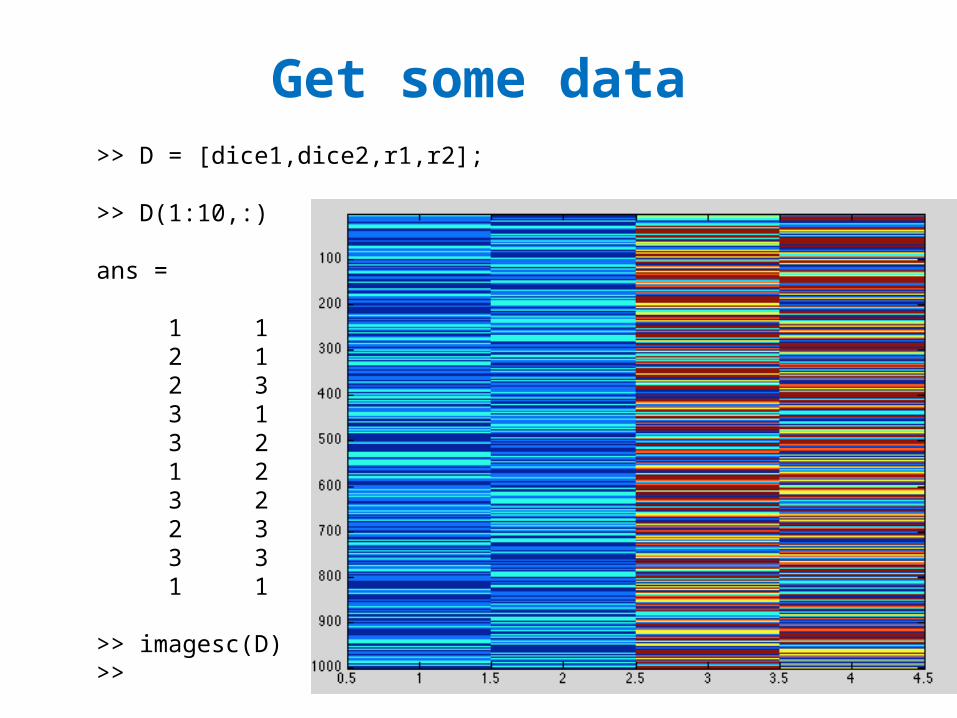
Get some data>> D = [dice1,dice2,r1,r2];
>> D(1:10,:)
ans =
1 1 7 4 2 1 1 3 2 3 1 1 3 1 1 2 3 2 2 1 1 2 4 7 3 2 2 1 2 3 7 2 3 3 1 2 1 1 3 6
>> imagesc(D)>>
Get some data
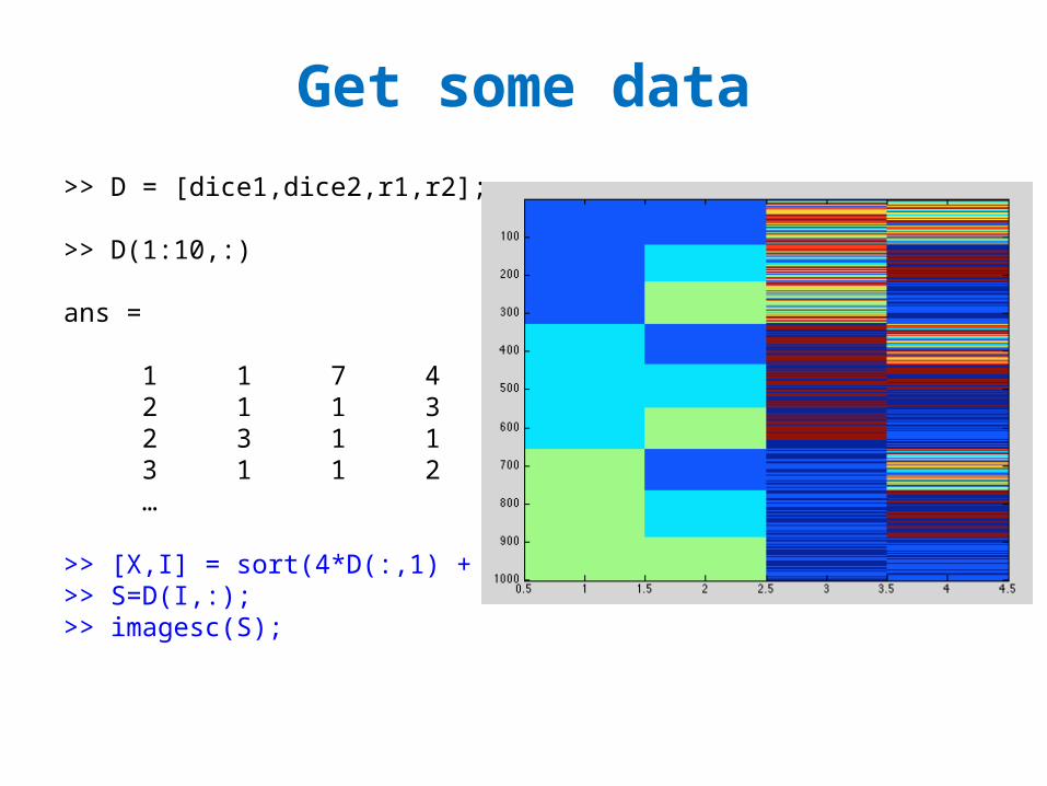
>> D = [dice1,dice2,r1,r2];
>> D(1:10,:)
ans =
1 1 7 4 2 1 1 3 2 3 1 1 3 1 1 2 …
>> [X,I] = sort(4*D(:,1) + D(:,2));>> S=D(I,:);>> imagesc(S);
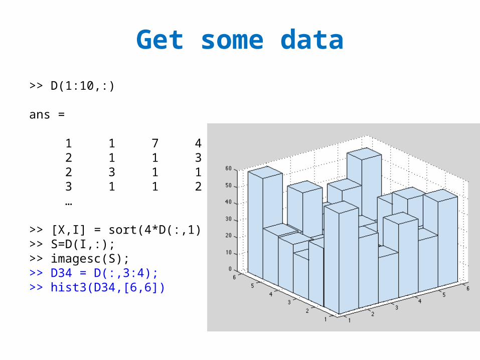
Get some data
>> D(1:10,:)
ans =
1 1 7 4 2 1 1 3 2 3 1 1 3 1 1 2 …
>> [X,I] = sort(4*D(:,1) + D(:,2));>> S=D(I,:);>> imagesc(S);>> D34 = D(:,3:4);>> hist3(D34,[6,6])
Estimate a joint density
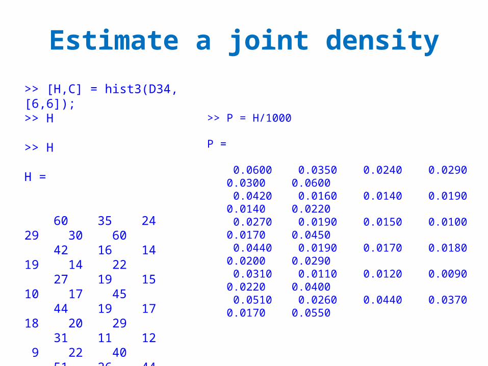
>> [H,C] = hist3(D34,[6,6]);>> H
>> H
H =
60 35 24 29 30 60 42 16 14 19 14 22 27 19 15 10 17 45 44 19 17 18 20 29 31 11 12 9 22 40 51 26 44 37 17 55
>> P = H/1000 P =
0.0600 0.0350 0.0240 0.0290 0.0300 0.0600 0.0420 0.0160 0.0140 0.0190 0.0140 0.0220 0.0270 0.0190 0.0150 0.0100 0.0170 0.0450 0.0440 0.0190 0.0170 0.0180 0.0200 0.0290 0.0310 0.0110 0.0120 0.0090 0.0220 0.0400 0.0510 0.0260 0.0440 0.0370 0.0170 0.0550
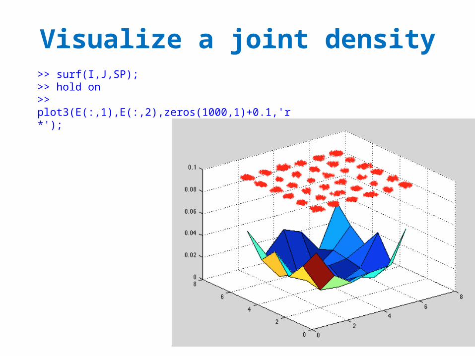
Visualize a joint density>> surf(I,J,SP);>> hold on>> plot3(E(:,1),E(:,2),zeros(1000,1)+0.1,'r*');
Inference with the joint
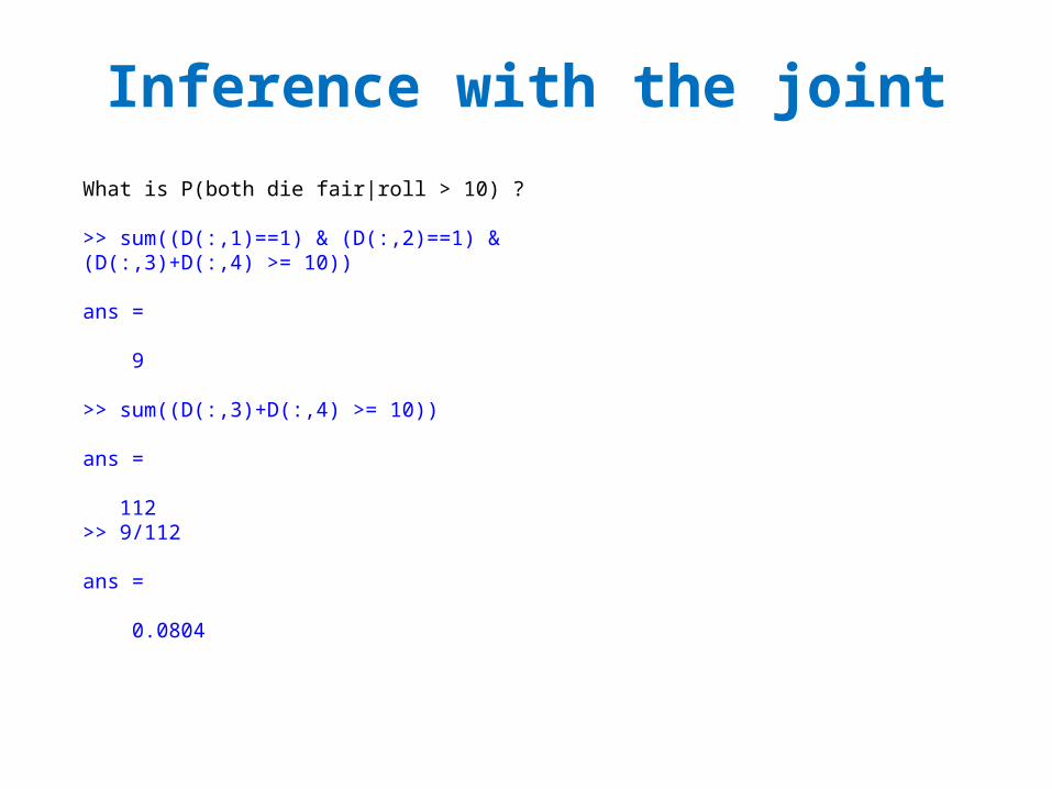
What is P(both die fair|roll > 10) ?
>> sum((D(:,1)==1) & (D(:,2)==1) & (D(:,3)+D(:,4) >= 10))
ans =
9
>> sum((D(:,3)+D(:,4) >= 10))
ans =
112>> 9/112
ans =
0.0804
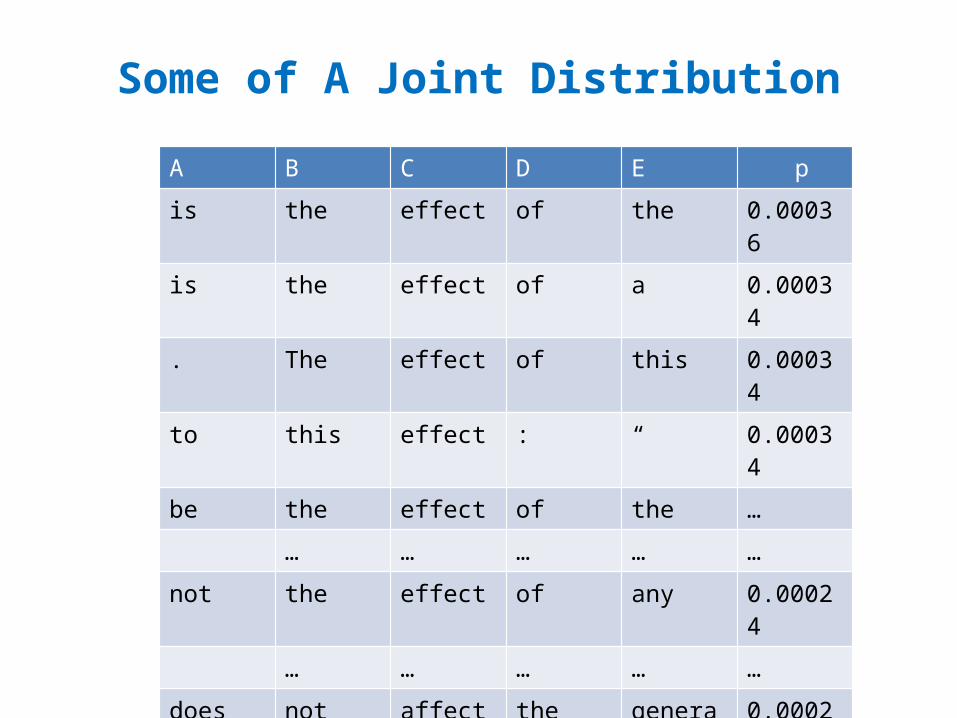
Some of A Joint DistributionA B C D E
p
is the effect of the 0.00036
is the effect of a 0.00034
. The effect of this 0.00034
to this effect : “ 0.00034
be the effect of the …
… … … … …
not the effect of any 0.00024
… … … … …
does not affect the general 0.00020
does not affect the question
0.00020
any manner affect the principle
0.00018
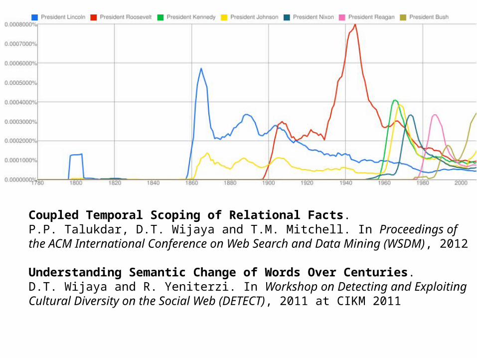
Coupled Temporal Scoping of Relational Facts. P.P. Talukdar, D.T. Wijaya and T.M. Mitchell. In Proceedings of the ACM International Conference on Web Search and Data Mining (WSDM), 2012
Understanding Semantic Change of Words Over Centuries. D.T. Wijaya and R. Yeniterzi. In Workshop on Detecting and Exploiting Cultural Diversity on the Social Web (DETECT), 2011 at CIKM 2011

Some of A Joint DistributionA B C D E
p
is the effect of the 0.00036
is the effect of a 0.00034
. The effect of this 0.00034
to this effect : “ 0.00034
be the effect of the …
… … … … …
not the effect of any 0.00024
… … … … …
does not affect the general 0.00020
does not affect the question
0.00020
any manner affect the principle
0.00018
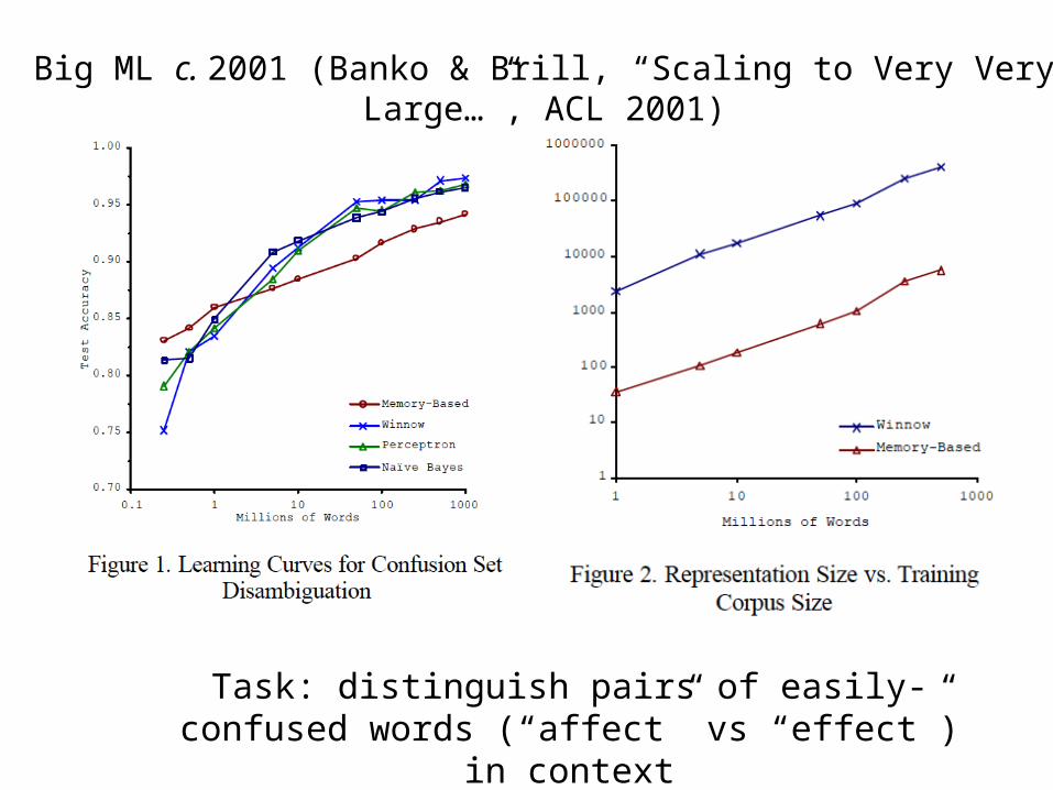
Big ML c. 2001 (Banko & Brill, “Scaling to Very Very Large…”, ACL 2001)
Task: distinguish pairs of easily-confused words (“affect” vs “effect”) in context
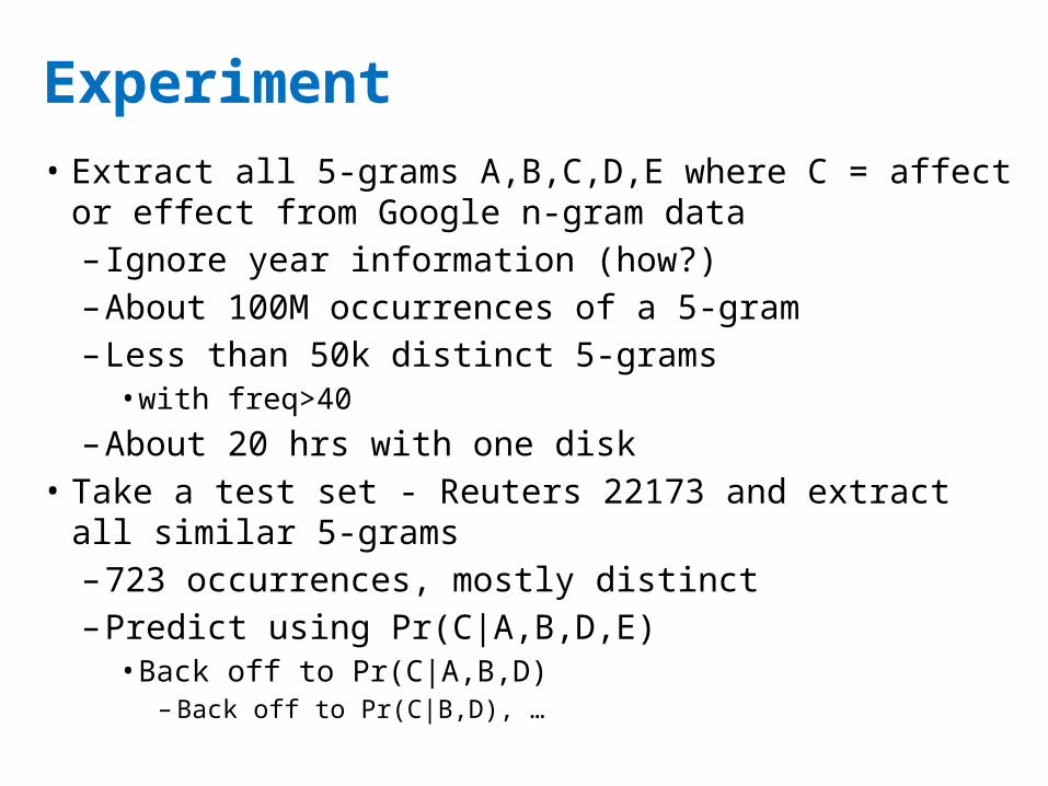
Experiment• Extract all 5-grams A,B,C,D,E where C = affect or
effect from Google n-gram data– Ignore year information (how?)– About 100M occurrences of a 5-gram– Less than 50k distinct 5-grams
• with freq>40
– About 20 hrs with one disk• Take a test set - Reuters 22173 and extract all
similar 5-grams– 723 occurrences, mostly distinct– Predict using Pr(C|A,B,D,E)
• Back off to Pr(C|A,B,D)– Back off to Pr(C|B,D), …
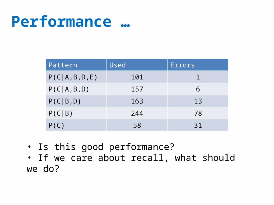
Performance …
Pattern Used Errors
P(C|A,B,D,E) 101 1
P(C|A,B,D) 157 6
P(C|B,D) 163 13
P(C|B) 244 78
P(C) 58 31
• Is this good performance?• If we care about recall, what should we do?

More from Andrew Moore’s slides…
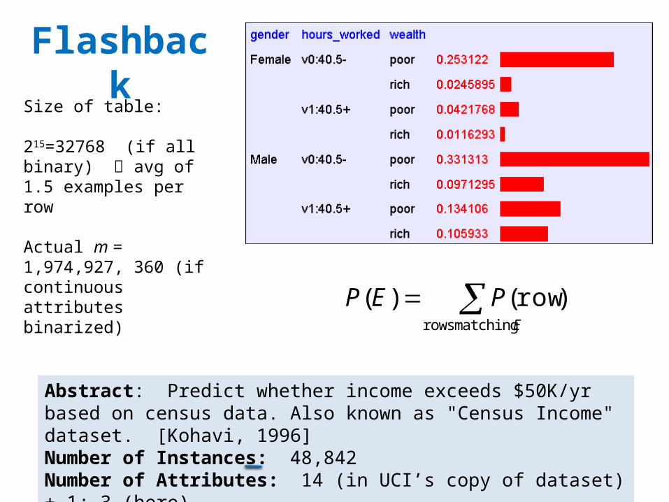
Flashback
E
PEP matching rows
)row()(
Abstract: Predict whether income exceeds $50K/yr based on census data. Also known as "Census Income" dataset. [Kohavi, 1996]Number of Instances: 48,842 Number of Attributes: 14 (in UCI’s copy of dataset) + 1; 3 (here)
Size of table:
215=32768 (if all binary) avg of 1.5 examples per row
Actual m = 1,974,927, 360 (if continuous attributes binarized)
Copyright © Andrew W. Moore
Naïve Density Estimation
What’s an alternative to the joint distribution?
The naïve model generalizes strongly:
Assume that each attribute is distributed independently of any of the other attributes.
Copyright © Andrew W. Moore
Using the Naïve Distribution
• Once you have a Naïve Distribution you can easily compute any row of the joint distribution.
• Suppose A, B, C and D are independently distributed. What is P(A ^ ~B ^ C ^ ~D)?
Copyright © Andrew W. Moore
Using the Naïve Distribution
• Once you have a Naïve Distribution you can easily compute any row of the joint distribution.
• Suppose A, B, C and D are independently distributed. What is P(A ^ ~B ^ C ^ ~D)?
P(A) P(~B) P(C) P(~D)

Copyright © Andrew W. Moore
Naïve Distribution General Case• Suppose X1,X2,…,Xd are independently
distributed.
• So if we have a Naïve Distribution we can construct any row of the implied Joint Distribution on demand.
• How do we learn this?
)Pr(...)Pr(),...,Pr( 1111 dddd xXxXxXxX
Copyright © Andrew W. Moore
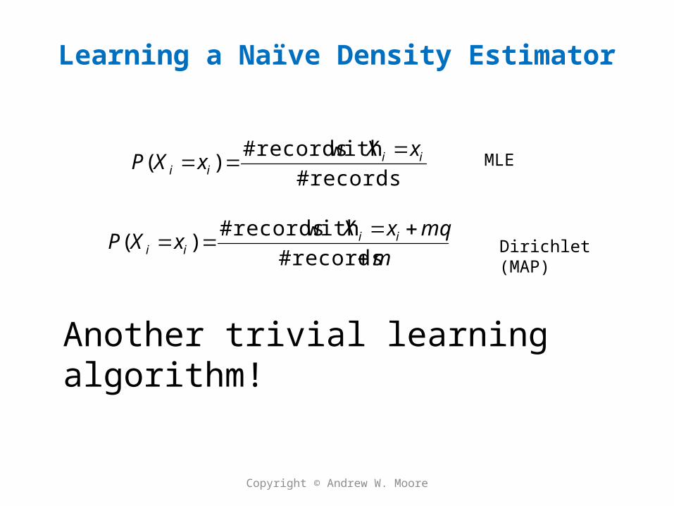
Learning a Naïve Density Estimator
Another trivial learning algorithm!
MLE
Dirichlet (MAP)
records#
with records#)( iiii
xXxXP
m
mqxXxXP iiii
records#
with records#)(
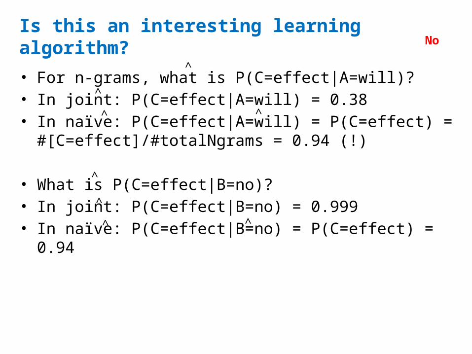
Is this an interesting learning algorithm?
• For n-grams, what is P(C=effect|A=will)?• In joint: P(C=effect|A=will) = 0.38• In naïve: P(C=effect|A=will) = P(C=effect) =
#[C=effect]/#totalNgrams = 0.94 (!)
• What is P(C=effect|B=no)?• In joint: P(C=effect|B=no) = 0.999• In naïve: P(C=effect|B=no) = P(C=effect) = 0.94
^
^
^ ^
^
^
^ ^
No
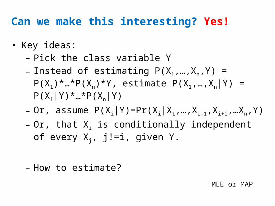
Can we make this interesting? Yes!
• Key ideas:– Pick the class variable Y– Instead of estimating P(X1,…,Xn,Y) = P(X1)*…
*P(Xn)*Y, estimate P(X1,…,Xn|Y) = P(X1|Y)*…*P(Xn|Y)
– Or, assume P(Xi|Y)=Pr(Xi|X1,…,Xi-1,Xi+1,…Xn,Y)
– Or, that Xi is conditionally independent of every Xj, j!=i, given Y.
– How to estimate?
MLE or MAP
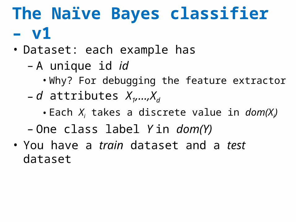
The Naïve Bayes classifier – v1• Dataset: each example has– A unique id id• Why? For debugging the feature extractor
– d attributes X1,…,Xd
• Each Xi takes a discrete value in dom(Xi)
– One class label Y in dom(Y)• You have a train dataset and a test dataset
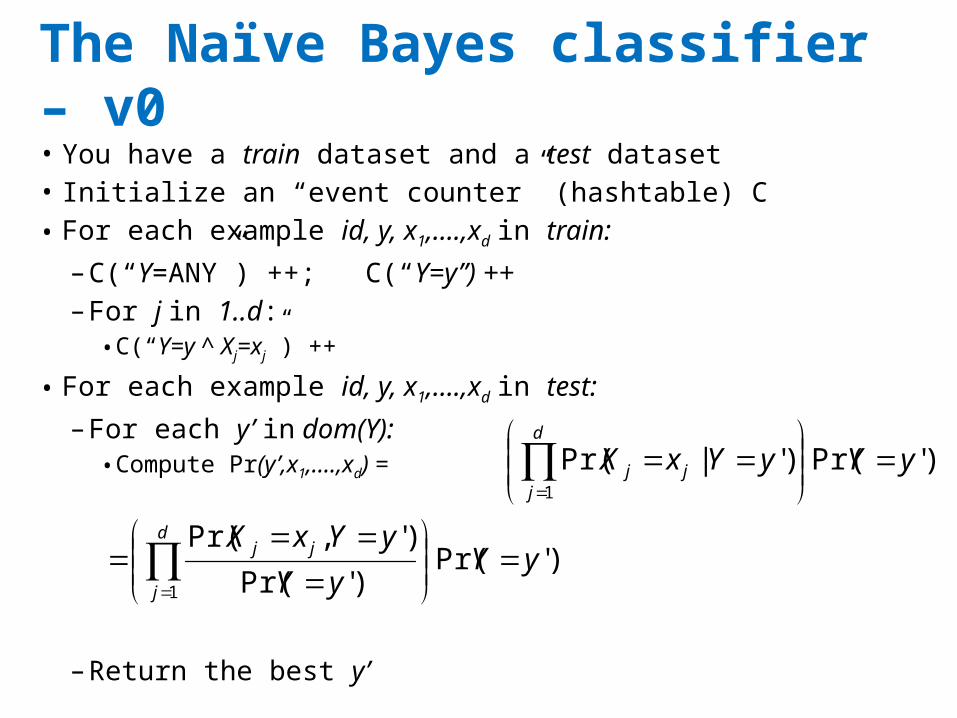
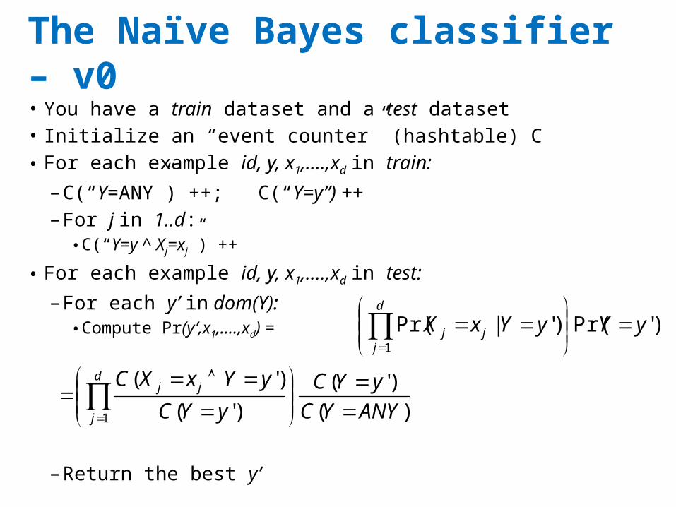
The Naïve Bayes classifier – v0• You have a train dataset and a test dataset• Initialize an “event counter” (hashtable) C• For each example id, y, x1,….,xd in train:
– C(“Y=ANY”) ++; C(“Y=y”) ++– For j in 1..d:
• C(“Y=y ^ Xj=xj”) ++
• For each example id, y, x1,….,xd in test:
– For each y’ in dom(Y):• Compute Pr(y’,x1,….,xd) =
– Return the best y’
)'Pr()'|Pr(1
yYyYxXd
jjj
)'Pr()'Pr(
)',Pr(
1
yYyY
yYxXd
j
jj
The Naïve Bayes classifier – v0• You have a train dataset and a test dataset• Initialize an “event counter” (hashtable) C• For each example id, y, x1,….,xd in train:
– C(“Y=ANY”) ++; C(“Y=y”) ++– For j in 1..d:
• C(“Y=y ^ Xj=xj”) ++
• For each example id, y, x1,….,xd in test:
– For each y’ in dom(Y):• Compute Pr(y’,x1,….,xd) =
– Return the best y’
)'Pr()'|Pr(1
yYyYxXd
jjj
)(
)'(
)'(
)'(
1 ANYYC
yYC
yYC
yYxXCd
j
jj
In-class demo
• Pilfered from Tom Mitchell
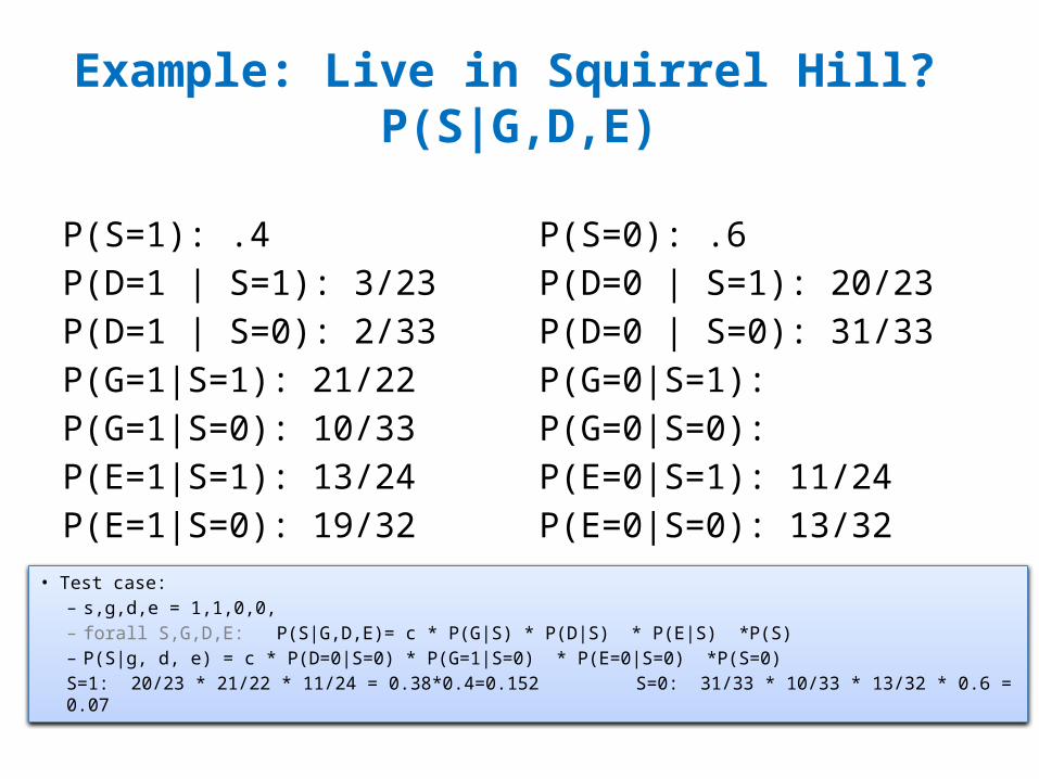
Example: Live in Squirrel Hill? P(S|G,D,E)
P(S=1): .4P(D=1 | S=1): 3/23P(D=1 | S=0): 2/33P(G=1|S=1): 21/22P(G=1|S=0): 10/33P(E=1|S=1): 13/24P(E=1|S=0): 19/32
P(S=0): .6P(D=0 | S=1): 20/23P(D=0 | S=0): 31/33P(G=0|S=1):P(G=0|S=0):P(E=0|S=1): 11/24P(E=0|S=0): 13/32
• Test case:– s,g,d,e = 1,1,0,0,– forall S,G,D,E: P(S|G,D,E)= c * P(G|S) * P(D|S) * P(E|S) *P(S)– P(S|g, d, e) = c * P(D=0|S=0) * P(G=1|S=0) * P(E=0|S=0) *P(S=0)S=1: 20/23 * 21/22 * 11/24 = 0.38*0.4=0.152 S=0: 31/33 * 10/33 * 13/32 * 0.6 = 0.07
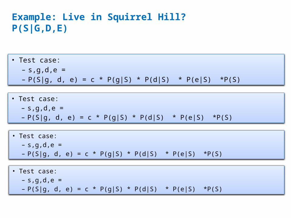
Example: Live in Squirrel Hill? P(S|G,D,E)
• Test case:– s,g,d,e = – P(S|g, d, e) = c * P(g|S) * P(d|S) * P(e|S) *P(S)
• Test case:– s,g,d,e = – P(S|g, d, e) = c * P(g|S) * P(d|S) * P(e|S) *P(S)
• Test case:– s,g,d,e = – P(S|g, d, e) = c * P(g|S) * P(d|S) * P(e|S) *P(S)
• Test case:– s,g,d,e = – P(S|g, d, e) = c * P(g|S) * P(d|S) * P(e|S) *P(S)

The Naïve Bayes classifier – v0• You have a train dataset and a test dataset• Initialize an “event counter” (hashtable) C• For each example id, y, x1,….,xd in train:
– C(“Y=ANY”) ++; C(“Y=y”) ++– For j in 1..d:
• C(“Y=y ^ Xj=xj”) ++
• For each example id, y, x1,….,xd in test:
– For each y’ in dom(Y):• Compute Pr(y’,x1,….,xd) =
– Return the best y’
)'Pr()'|Pr(1
yYyYxXd
jjj
)(
)'(
)'(
)'(
1 ANYYC
yYC
yYC
yYxXCd
j
jj
This may overfit, so …
The Naïve Bayes classifier – v1• You have a train dataset and a test dataset• Initialize an “event counter” (hashtable) C• For each example id, y, x1,….,xd in train:
– C(“Y=ANY”) ++; C(“Y=y”) ++– For j in 1..d:
• C(“Y=y ^ Xj=xj”) ++
• For each example id, y, x1,….,xd in test:
– For each y’ in dom(Y):• Compute Pr(y’,x1,….,xd) =
– Return the best y’
)'Pr()'|Pr(1
yYyYxXd
jjj
mANYYC
mqyYC
myYC
mqyYxXC jd
j
jjj
)(
)'(
)'(
)'(
1
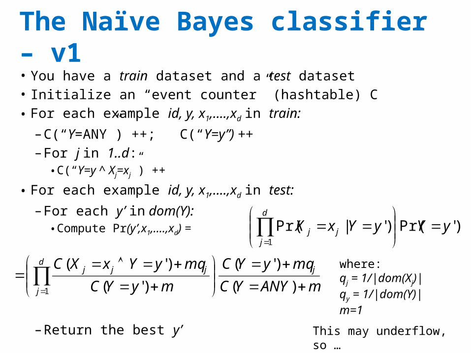
where:qj = 1/|dom(Xj)|qy = 1/|dom(Y)|m=1
This may underflow, so …
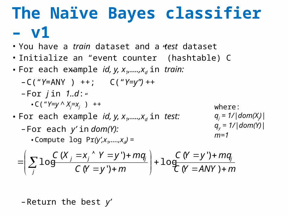
The Naïve Bayes classifier – v1• You have a train dataset and a test dataset• Initialize an “event counter” (hashtable) C• For each example id, y, x1,….,xd in train:
– C(“Y=ANY”) ++; C(“Y=y”) ++– For j in 1..d:
• C(“Y=y ^ Xj=xj”) ++
• For each example id, y, x1,….,xd in test:
– For each y’ in dom(Y):• Compute log Pr(y’,x1,….,xd) =
– Return the best y’
mANYYC
mqyYC
myYC
mqyYxXC j
j
jjj
)(
)'(log
)'(
)'(log
where:qj = 1/|dom(Xj)|qy = 1/|dom(Y)|m=1
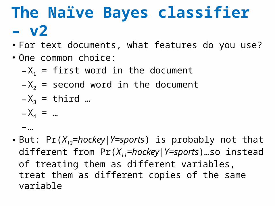
The Naïve Bayes classifier – v2• For text documents, what features do you use?• One common choice:– X1 = first word in the document
– X2 = second word in the document
– X3 = third …
– X4 = …
–…• But: Pr(X13=hockey|Y=sports) is probably not that
different from Pr(X11=hockey|Y=sports)…so instead of treating them as different variables, treat them as different copies of the same variable

The Naïve Bayes classifier – v1• You have a train dataset and a test dataset• Initialize an “event counter” (hashtable) C• For each example id, y, x1,….,xd in train:
– C(“Y=ANY”) ++; C(“Y=y”) ++– For j in 1..d:
• C(“Y=y ^ Xj=xj”) ++
• For each example id, y, x1,….,xd in test:
– For each y’ in dom(Y):• Compute Pr(y’,x1,….,xd) =
– Return the best y’
)'Pr()'|Pr(1
yYyYxXd
jjj
)'Pr()'Pr(
)',Pr(
1
yYyY
yYxXd
j
jj
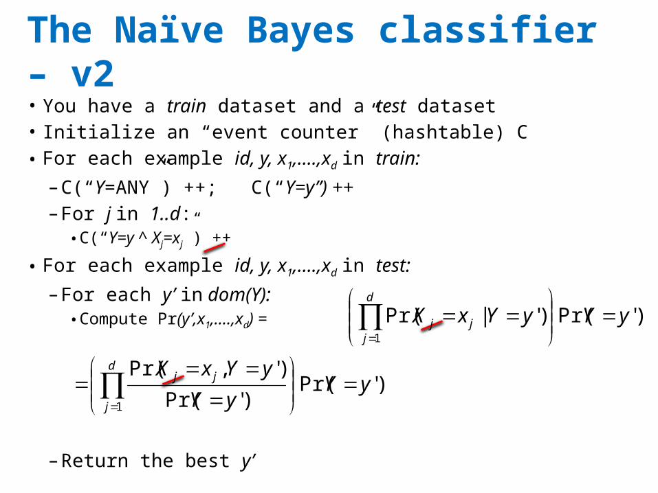
The Naïve Bayes classifier – v2• You have a train dataset and a test dataset• Initialize an “event counter” (hashtable) C• For each example id, y, x1,….,xd in train:
– C(“Y=ANY”) ++; C(“Y=y”) ++– For j in 1..d:
• C(“Y=y ^ Xj=xj”) ++
• For each example id, y, x1,….,xd in test:
– For each y’ in dom(Y):• Compute Pr(y’,x1,….,xd) =
– Return the best y’
)'Pr()'|Pr(1
yYyYxXd
jjj
)'Pr()'Pr(
)',Pr(
1
yYyY
yYxXd
j
jj

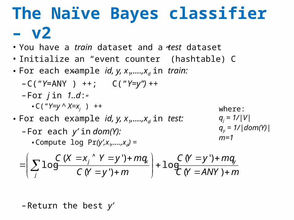
The Naïve Bayes classifier – v2• You have a train dataset and a test dataset• Initialize an “event counter” (hashtable) C• For each example id, y, x1,….,xd in train:
– C(“Y=ANY”) ++; C(“Y=y”) ++– For j in 1..d:
• C(“Y=y ^ X=xj”) ++
• For each example id, y, x1,….,xd in test:
– For each y’ in dom(Y):• Compute Pr(y’,x1,….,xd) =
– Return the best y’
)'Pr()'|Pr(1
yYyYxXd
jj
)'Pr()'Pr(
)',Pr(
1
yYyY
yYxXd
j
j
The Naïve Bayes classifier – v2• You have a train dataset and a test dataset• Initialize an “event counter” (hashtable) C• For each example id, y, x1,….,xd in train:
– C(“Y=ANY”) ++; C(“Y=y”) ++– For j in 1..d:
• C(“Y=y ^ X=xj”) ++
• For each example id, y, x1,….,xd in test:
– For each y’ in dom(Y):• Compute log Pr(y’,x1,….,xd) =
– Return the best y’
mANYYC
mqyYC
myYC
mqyYxXC y
j
xj
)(
)'(log
)'(
)'(log
where:qj = 1/|V|qy = 1/|dom(Y)|m=1
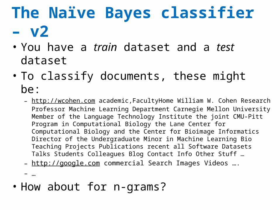
The Naïve Bayes classifier – v2• You have a train dataset and a test
dataset• To classify documents, these might be:
– http://wcohen.com academic,FacultyHome William W. Cohen Research Professor Machine Learning Department Carnegie Mellon University Member of the Language Technology Institute the joint CMU-Pitt Program in Computational Biology the Lane Center for Computational Biology and the Center for Bioimage Informatics Director of the Undergraduate Minor in Machine Learning Bio Teaching Projects Publications recent all Software Datasets Talks Students Colleagues Blog Contact Info Other Stuff …
– http://google.com commercial Search Images Videos ….– …
• How about for n-grams?
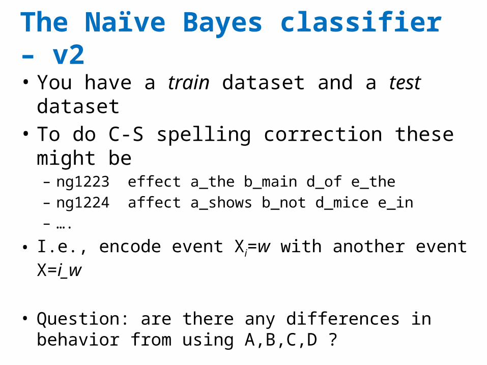
The Naïve Bayes classifier – v2• You have a train dataset and a test
dataset• To do C-S spelling correction these might
be– ng1223 effect a_the b_main d_of e_the– ng1224 affect a_shows b_not d_mice e_in– ….
• I.e., encode event Xi=w with another event X=i_w
• Question: are there any differences in behavior from using A,B,C,D ?
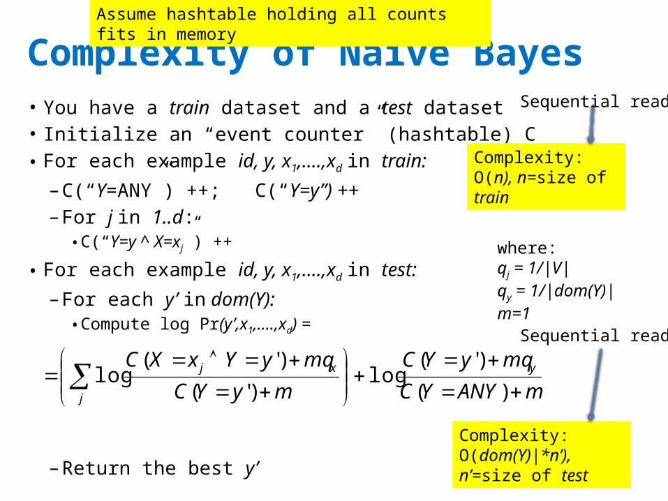
Complexity of Naïve Bayes• You have a train dataset and a test dataset• Initialize an “event counter” (hashtable) C• For each example id, y, x1,….,xd in train:
– C(“Y=ANY”) ++; C(“Y=y”) ++– For j in 1..d:
• C(“Y=y ^ X=xj”) ++
• For each example id, y, x1,….,xd in test:
– For each y’ in dom(Y):• Compute log Pr(y’,x1,….,xd) =
– Return the best y’
mANYYC
mqyYC
myYC
mqyYxXC y
j
xj
)(
)'(log
)'(
)'(log
where:qj = 1/|V|qy = 1/|dom(Y)|m=1
Complexity: O(n), n=size of train
Complexity: O(dom(Y)|*n’), n’=size of test
Assume hashtable holding all counts fits in memory
Sequential reads
Sequential reads
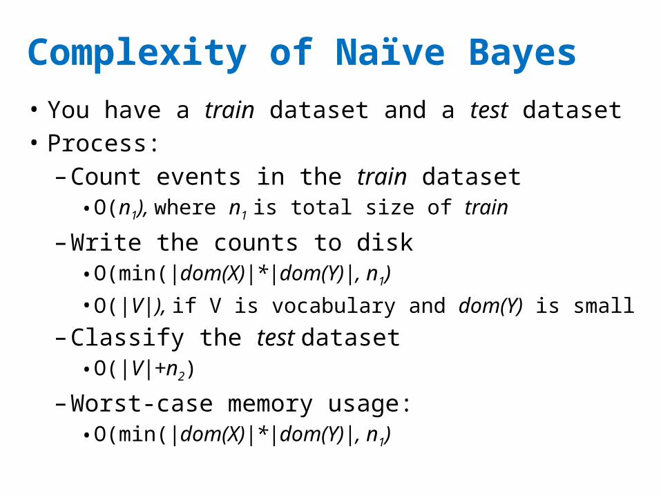
Complexity of Naïve Bayes• You have a train dataset and a test dataset• Process:– Count events in the train dataset• O(n1), where n1 is total size of train
–Write the counts to disk• O(min(|dom(X)|*|dom(Y)|, n1)
• O(|V|), if V is vocabulary and dom(Y) is small
– Classify the test dataset• O(|V|+n2)
–Worst-case memory usage:• O(min(|dom(X)|*|dom(Y)|, n1)
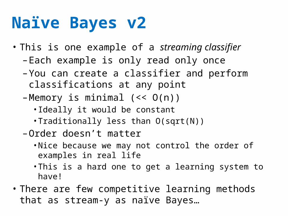
Naïve Bayes v2• This is one example of a streaming classifier– Each example is only read only once– You can create a classifier and perform
classifications at any point– Memory is minimal (<< O(n))
• Ideally it would be constant• Traditionally less than O(sqrt(N))
– Order doesn’t matter• Nice because we may not control the order of
examples in real life• This is a hard one to get a learning system to have!
• There are few competitive learning methods that as stream-y as naïve Bayes…
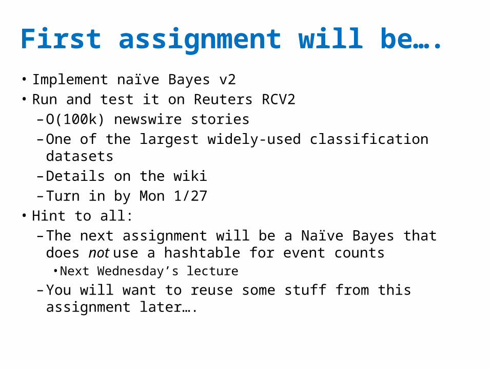
First assignment will be….• Implement naïve Bayes v2• Run and test it on Reuters RCV2– O(100k) newswire stories– One of the largest widely-used classification datasets– Details on the wiki– Turn in by Mon 1/27
• Hint to all:– The next assignment will be a Naïve Bayes that does
not use a hashtable for event counts• Next Wednesday’s lecture
– You will want to reuse some stuff from this assignment later….