N A S A T E C H N I C A L

R E P O R T

AFWL TECHNICAL KIRTLAND AFB,

4 7 3 &

-\ I

ROCKET EXHAUST EFFLUENT MODELING FOR TROPOSPHERIC AIR QUALITY A N D ENVIRONMENTAL ASSESSMENTS

r ­

t It , \

-7 . J. Briscoe Stephens a n d Roger B, Stewar$ 2-

George C. Marshal l Space Flight Center /

Marshall Space Flight Center, Ala. 35812

N A T I O N A L AERONAUTICS A N D SPACE A D M I N I S T R A T I O N W A S H I N G T O N , 0. C. JUNE 1977

- -

I . REPORTNO. 2. GOVERNMENT ACCESSION NO.

NASA TR R-473 Ii- . - . - - . 14 TITLE AND SUBTITLE

I Rocket Exhaust Effluent Modeling for Tropospheric Air Quality and Environmental Assessments

7. AUTHOR(S)

I[ J. Briscoe Stephens and Roger B. Stewart* 9. PERFORMING ORGANIZATION N A M E AND ADDRESS

George C. Marshall Space Flight Center Marshall Space Flight Center, Alabama 35812

112. SPONSORING AGENCY NAME AND ADDRESS

National Aeronautics and Space Administration Washington, D.C. 20546

iis. SUPPLEMENTARY NOTES /--

Prepared by Space Sciences Laboratory, Science and Engineering *Langley Research Center

16. ABSTRACT

5. REPORT DATE June 1977

6. PERFORMING ORGANIZATION CODE

8. PERFORMING ORGANIZATION REP0R.r 1

M-222~- ~

0 . WORK UNIT, NO.

11. CONTRACT OR GRANT NO.

13. T Y P E OF REPORi' & PERIOD COVERE

Technical Report 1 4 . SPONSORING AGENCY CODE

The various techniques for diffusion predictions to support air quality predictions and environmental assessments for aerospace applications are discussed in terms pf limitations imposed by atmospheric data. This affords an introduction to the rationale behind the selection of the National Aeronautics and Space Administration (NASA)/Marshall Space Flight Center (MSFC) Rocket Exhaust Effluent Diffusion (REED) program. The models utilized in the NASAlMSFC REED program are explained. This program is then evaluated in terms of some results from a joint MSFC/Langley Research Center/Kennedy Space Center Titan Exhaust Effluent Prediction and Monitoring Program.

18. OlSTRlBUTlON S T A T E M E N T

Diffusion modeling Atmospheric modeling Category: 34 Aerospace effluents

19. SECURITY CLASSIF . (of thlm rep&) 20. SECURITY CLA! IF. (ofthln page) 21. NO. O F PAGES 22. P R I C E

Unclassified Unclassified I 87 I $5.00 I I

ACKNOWLEDGMENTS

The authors wish to acknowledge the helpful advice and support of Dr. William W. Vaughan, Chief of the Aerospace Environmental Division of the Space Sciences Laboratory at Marshall Space Flight Center, and H. Scot Wagner, Chief of the Atmospheric Emironmen ts Branch at Langley Research Center. We also wish to thank Dr. G. L. Gregory of Langley Research Center, C. Warren Campbell of Marshall Space Flight Center, and A. I. Goldford and Dr. S. I. Adelfang of Science Applications, Inc., for their technical assistance in the preparation of this report.

To the many others whose names do not appear in this acknowledgment but whose efforts have contributed to the success of this work, we wish to express our gratitutde.

A paper based on the contents of this report was presented at the NASA Space Shuttle Tropospheric Environmental Effects Meeting, Langley, Virginia, February 24 through 26, 1975. Dr. Roger B. Stewart, Langley Research Center, was a coauthor of the paper. However, Dr. Stewart’s untimely death in 1976 prevented his participation in the final revision of the report for publication. His contributions were important and, accordingly, are recognized by retaining him as a coauthor of the report.

TABLE OF CONTENTS

Page

I. INTRODUCTION . . . . . . . . . . . . . . . . . . . . . . . 1

I1. A GENERAL DESCRIPTION OF THE PROBLEM . . . . . . . . . . . 2

A. Overview . . . . . . . . . . . . . . . . . . . . . . . . . 2 B. Meteorology . . . . . . . . . . . . . . . . . . . . . . . 4 C. Chemistry . . . . . . . . . . . . . . . . . . . . . . . . 5 D. Diffusive Transport . . . . . . . . . . . . . . . . . . . . . 7

I11. MODELING OF THE PHYSICAL PROCESSES ASSOCIATED WITH THE TRANSPORT OF ROCKET EXHAUST EFFLUENTS IN THE TROPOSPHERE . . . . . . . . . . . . . . . . . . . . . . . . . 9

A. Overview . . . . . . . . . . . . . . . . . . . . . . . . . 9 B. Meteorological Modeling . . . . . . . . . . . . . . . . . . . 11 C. Modeling of the Rocket Exhaust Effluent Chemistry . . . . . . . . 13 D. Modeling of the Transport of Rocket Exhaust Effluents in the

Troposphere . . . . . . . . . . . . . . . . . . . . . . . 16 E. Applications . . . . . . . . . . . . . . . . . . . . . . . 20

IV. NASA/MSFC ROCKET EXHAUST EFFLUENT DIFFUSION (REED) DESCRIPTION . . . . . . . . . . . . . . . . . . . . . . . . 21

A. Overview of the NASAlMSFC REED Description . . . . . . . . . 22 B. NASAlMSFC Rocket Exhaust Cloud Rise Model . . . . . . . . . 24 C. NASAlMSFC Multilayer Diffusion Model . . . . . . . . . . . . 30 D. Real-Time Diffusion Predictions . . . . . . . . . . . . . . . . 53

V . TITANEXHAUSTEFFLUENTMONITORINGPROGRAM . . . . . . 57

A. Titan Exhaust Cloud Transport and Transit . . . . . . . . . . . . 58 B. Airborne Measurements and Cloud Chemistry . . . . . . . . . . . 60 C. Surface Monitoring . . . . . . . . . . . . . . . . . . . . . 64

VI. .CONCLUDING COMMENTS . . . . . . . . . . . . . . . . . . . 67

REFERENCES . . . . . . . . . . . . . . . . . . . . . . . . . . . 69

iii

1

2

3

4

5

6

7

8

9

10

11

12

13

14

15

16

17

LIST OF ILLUSTRATIONS

Figure

.

.

.

.

.

.

.

.

.

.

.

.

.

.

.

.

.

18.

19.

Title

Viking B. Titan-Centaur launch. September 9. 1975 (T + 7 s) . .

Viking B. Titan-Centaur launch. September 9. 1975 (T + 30 s). .

Schematic of rocket exhaust ground cloud formation and transport

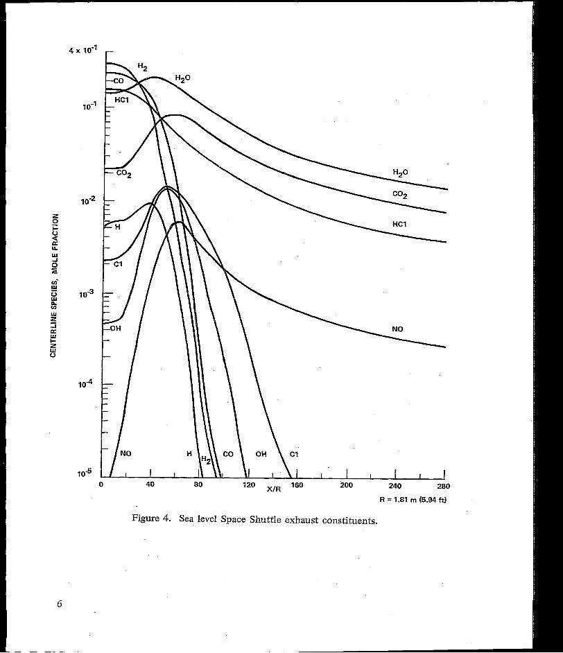
Sea level Space Shuttle exhaust constituents . . . . . . . . .

Devices for atmospheric soundings . . . . . . . . . . . . .

Bimodal rocket exhaust effluent chemistry . . . . . . . . . .

Selection of a general diffusion model . . . . . . . . . . . .

Comparison between Gaussian and square wave distributions . . .

NASA/MSFC REED description . . . . . . . . . . . . . .

Exhaust cloud stabilization . . . . . . . . . . . . . . . .

NASA/MSFC multilayer diffusion model . . . . . . . . . .

Source cloud distribution . . . . . . . . . . . . . . . .

Effects of version V spline fit on isopleth . . . . . . . . . .

Page

. . . 2

. . . 3

. . . 5

. . . 6

. . . 11

. . . 14

. . . 16

. . . 19

. . . 22

. . 24

. . 33

. . . 37

. . . 37

a-and y-aluminacollected from solid rocket exhaust . . . . . . . . . 41

NASA/MSFC REEDA system . . . . . . . . . . . . . . . . . . 54

Atmospheric conditions at launch time (T-0) . . . . . . . . . . . . 55

Predicted exhaust effluent cloud rise history for launch atmosphere (T-0) . . . . . . . . . . . . . . . . . . . . . . . 56

Model 3 launch prediction for the centerline concentrations and dosages (T-0) . . . . . . . . . . . . . . . . . . . . . . . . 56

Model 3 launch prediction for the HCl isopleths (T-0) . . . . . . . . . 57

iv

11.11111.1111 ............................................. '

LIST OF ILLUSTRATIONS (Concluded)

Figure Title Page

20. Ground cloud rise to stabilization . . . . . . . . . . . . . . . . 58

21. Ground cloud track, Titan I11 launch, May 30, 1974 . . . . . . . . . 59

22. February 11, 1974, measured Titan-Centaur ground cloud growth . . . . 60

23. Turbulent mixing - finite rate rocket plume calculation of sea level nitric oxide production from Titan I11 booster with N2O4 TVC injection . . . 6 1

24. Titan III-C ATS-F launch, May 30, 1974 . . . . . . . . . . . . . . 62

25. Airborne hydrogen chloride measurements, December 10, 1974, aircraft flight speed = 5 1 m/s . . . . . . . . . . . . . . . . . . 63

26. Hydrogen chloride ground measurement, chemiluminescent (method I), December 10, 1 9 7 4 . . . . . . . . . . . . . . . . . . . . . . 65

27. Measured ground cloud crosswind growth, February 11, 1974, Titan-Centaur and December 10, 1974, Titan-Helios . . . . . . . . . 67

V

H

K

CP

f

g

h

m

P

9

LIST OF SYMBOLS AND DEFINITIONS

Symbols

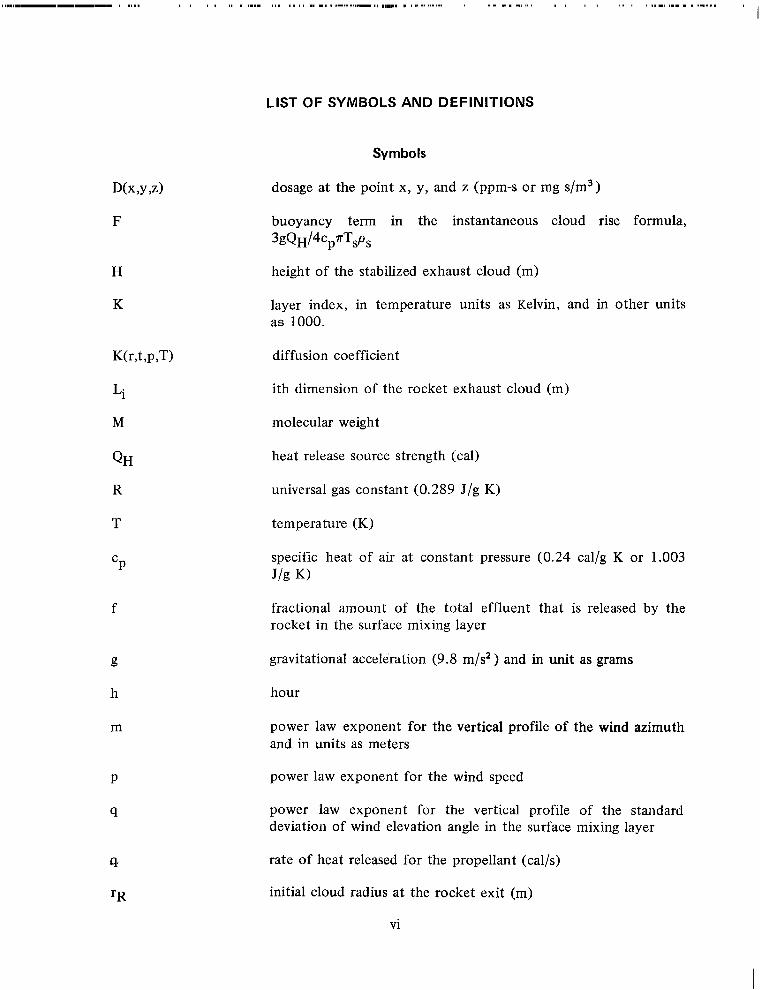
dosage at the point x, y, and z (ppm-s or mg s/m3)

buoyancy term in the instantaneous cloud rise formula,

height of the stabilized exhaust cloud (m)

layer index, in temperature units as Kelvin, and in other units as 1000.

diffusion coefficient

ith dimension of the rocket exhaust cloud (m)

molecular weight

heat release source strength (cal)

universal gas constant (0.289 J/g K)

temperature (K)

specific heat of air at constant pressure (0.24 cal/g K or 1.003 J/g K)

fractional amount of the total effluent that is released by the rocket in the surface mixing layer

gravitational acceleration (9.8 m/s2) and in unit as grams

hour

power law exponent for the vertical profile of the wind azimuth and in units as meters

power law exponent for the wind speed

power law exponent for the vertical profile of the standard deviation of wind elevation angle in the surface mixing layer

rate of heat released for the propellant (cal/s)

initial cloud radius at the rocket exit (m)

vi

S

t

-U

<U>

Y

Z

a

P

Y

P

a~~

a~~

OER

a~~

r

aa /az

A

LIST OF SYMBOLS AND DEFINITIONS (Continued)

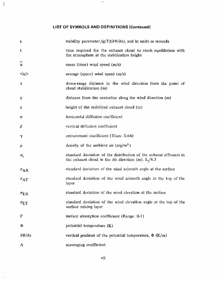
stability parameter,(g/T)(a@/az), and in units as seconds

time required for the exhaust cloud to reach equilibrium with the atmosphere at the stabilization height

mean (time) wind speed (m/s)

average (space) wind speed (m/s)

down-range distance in the wind direction from the point of cloud stabilization (m)

distance from the centerline along the wind direction (m)

height of the stabilized exhaust cloud (m)

horizontal diffusion coefficient

vertical diffusion coefficient

entrainment coefficient (Titan: 0.64)

density of the ambient air (mg/m3)

standard deviation of the distribution of the exhaust effluents in the exhaust cloud in the ith direction (m), Li/4.3

standard deviation of the wind azimuth angle at the surface

standard deviation of the wind azimuth angle at the top of the layer

standard deviation of the wind elevation at the surface

standard deviation of the wind elevation angle at the top of the surface mixing layer

surface absorption coefficient (Range: 0-1)

potential temperature (K)

vertical gradient of the potential temperature, (K/m)

scavenging coefficient

vii

X

LIST OF SYMBOLS AND DEFINITIONS (Continued)

Centerline

Concentration

Dosage

Ground Cloud

Plume Cloud

Potential Temperature (a)

Quasi-adiabatic Layer

Stable Layer

Transport Layer

change in wind direction between the top and bottom of the surface mixing layer, 8T - OB

total mass source strength (ppm or mg/m3)

the mass source strength in the ith layer (ppm or mg/m3)

the concentration (ppm or mg/m3)

Terms

The radial vector in the direction of the mean wind direction whose origin is the launch site.

The amount of the effluent present at a specific time. The average concentration is the average amount present during the event.

The measure of the total amount of effluent (time integrated concentration) due to the vehicle launch at a specific location.

That cloud of rocket effluents emitted during the initial phase of vehicle launch. This cloud is assumed to have an ellipsoidal shape and is normally in the surface transport layer.

The cloud of rocket effluents emitted from the vehicle in flight. This cloud has a cylindrical shape whose height is defined by the vertical thickness of the layer and is normally above the surface transport layer.

The temperature a volume of dry air would have if brought adiabatically from its initial state to the standard pressure of 1000 mb.

A layer in which the vertical potential temperature gradient is zero or less.

A layer in which the vertical potential temperature gradient is positive .

An atmospheric layer within which the diffusion process is constrained.

viii

LIST OF SYMBOLS AND DEFINITIONS (Concluded)

Acronyms

REED Description -Rocket Exhaust Effluent Diffusion description. This includes all models; i.e., meteorological model, cloud rise model, and multilayer diffusion model.

REEDA System socket Exhaust Effluent _Diffusion Analysis. This is a computer with peripherals used to make diffusion calculations using the REED description.

PET Polychromatic Enhanced Terminal. 'This is a proposed colored interactive terminal that could interface to the REEDA system.

ix

ROCKET EXHAUST EFFLUENT MODELING FOR TROPOSPHERIC AIR QUALITY AND ENVIRONMENTAL ASSESSMENTS

1. INTRODUCTION

The approach and status of investigations, together with the future requirements for the development of an operational model, for the description of rocket exhaust effluent transport are discussed herein. Such a model is important for the environmental assessment for aerospace vehicles. The primary objective is an analytical description of the transport and downwind ground-level concentration of aerospace effluents from solid rocket boosters, e.g., hydrogen chloride (HCl) and aluminum oxide (Al, 0,).

Modeling of rocket exhaust effluent transport for air quality and environmental assessments is in progress to provide a better understanding of the various input and output parameter interactions relative to aerospace activities. An effective transport model requires an integration of atmospheric dynamics within the surface transport layer with the rocket exhaust chemical reactions and the turbulent diffusion. To ensure public safety [ 1,2] the National Aeronautics and Space Administration (NASA) has conducted and is conducting environmental assessments of the effects for aerospace operations [3-lo]. Because of the planned high utilization of the Space Shuttle, special consideration is given to the environmental effects of this vehicle [ 11I ; thus, the Space Shuttle may serve as a model for all aerospace environmental assessments. The tropospheric environmental effects modeling program has advanced to the research operational stage. Each section of this report is prefaced with an overview of the subjects to be discussed with supporting technical details in the subsequent parts.

The monitoring of large scale rocket launches provides a data base for transport model refinements, as well as empirical support for the transport model predictions. Launch monitoring also provides verification of results obtained in laboratory and chamber studies. Finally, the NASA Centers' joint rocket launch prediction and monitoring program provides scientific data base for the agency.

The present tropospheric environmental program is being carried out by five NASA field centers: coordination is provided by Johnson Space Center (JSC); chamber tests, diffusion modeling development and real-time transport forecasts are conducted by Marshall Space Flight Center (MSFC); launch' monitoring, laboratory studies, and analytical chemical studies are performed by Langley Research Center (LaRC); operational monitoring support and bio-medical investigations are conducted by Kennedy Space Center (KSC); and additional airborne monitoring and basic chemical kinetic studies are conducted by Ames Research Center (ARC). In addition, basic research concerning particulate behavior is underway at the Jet Propulsion Laboratory (JPL). University and industrial investigations are also being supported by the agency.

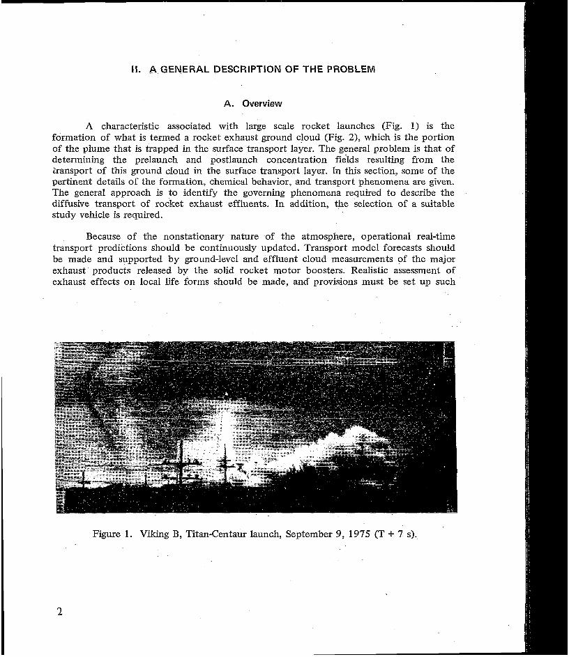
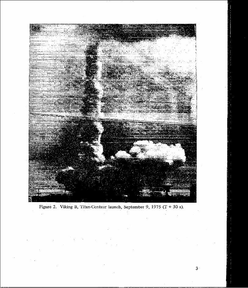
Figure 2. Viking B, Titan-Centaur launch, September 9, 1975 (T + 30 s).

3

that any potential launch constraints can be clearly identified during the space vehicle launch sequences. Finally, a need exists for investigating potential ecological impact resulting from acid rain (washout) from the ground cloud.

Laboratory and chamber experiments can provide fundamental information on distinct (idealized) aspects of the cloud physics and chemistry; however, monitoring of large-scale rocket exhaust clouds is needed to relate these studies to the stochastic problems in the atmosphere. The above statements lead directly to consideration of candidate solid rocket booster test vehicles. Primary emphasis must be placed on studying boosters having propellant chemical formulations similar to the Space Shuttle booster solid propellant. To alleviate size scaling problems, a large study vehicle is desirable. These requirements lead to the selection of Titan I11 solid rocket boosters as study vehicles. The discussion that follows refers to our present knowledge of the formation of rocket-produced ground clouds from these vehicles. The Titan I11 solid boosters are about one-half the size of Shuttle boosters. There are no liquid engines burning a t lift-off on the Titan as are present on Shuttle; however, Shuttle liquid engines produce water vapor as the major exhaust constituent and may affect the formation of aqu’eous hydrogen chloride and cause synergistic effects with the aluminum oxide.

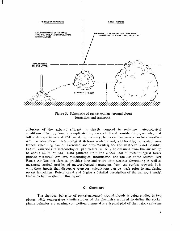
The formation of such rocket exhaust ground clouds can be outlined by considering typical rocket parameters. The exhaust plume initially impinges on the launch complex structure, a flame deflector and water filled trench. The clouds are formed from high temperature combustion products (exit plane temperatures of about 2146 K) and vaporized flame trench water. The hot exhaust clouds rise, radiating energy, to an altitude at which buoyant equilibrium with the ambient atmosphere is established (typically 1 to 2 km above the Earth’s surface) in a period of 5 to 10 min after launch and commence the transport phase while drifting with the average wind speed. At stabilization the clouds typically contain 99.9 percent of their mass as ambient air entrained during the rise portion of their trajectory. The major rocket exhaust constituents are hydrogen chloride (HCl), carbon dioxide (CO, ), water vapor (H,O), aluminum oxide (AlpOs), hydrogen (H,), carbon monoxide (CO), and chlorine (Cl,), where only HC1 and Al,O3 are of primary interest environmentally. Chemical kinetic rocket plume claculations indicate that virtually all of the molecular hydrogen and carbon monoxide are afterburned to produce HzO, OH, and CO,. Figure 3 is a schematic representation of the formation and transport process of such clouds. The early cloud rise, growth, and stabilization, as well as ’the diffusive transport along the mean wind, are problems intimately coupled to small scale meteorological phenomena, rocket plume chemistry, exhaust cloud chemistry, and turbulent diffusion. Added to these physical problems are the difficulties involved in carrying out launch monitoring experiments.

B. Meteorology

Meteorological documentation of wind field dynamics, thermodynamics, and statistical properties for diffusion studies has received extensive study during the past two decades as indicated by References 12 through 18. The problem of forecasting the

4

I

THERMODYNAMIC MODE KlNECTlC MODE

CLOUD DYNAMICS DETERMINED INITIAL CONDITIONS FOR DISPERSIVEFROM BUOYANCY AND MOMENTUM TRANSPORTOFROCKETGROUNDCLOUDCONSERVATION

ATMOSPHERIC MIXING LAYER

STABILIZED CLOUD

Figure 3. Schematic of rocket exhaust ground cloud formation and transport.

diffusion of the exhaust effluents is strictly coupled to real-time meteorological conditions. The problem is complicated by two additional considerations; namely, that full scale experiments at KSC must, by necessity, be carried out near a land-sea interface with no ocean-based meteorological stations available and, additionally, no control over launch scheduling can be exercised and thus “waiting for the weather” is not possible. Lateral variations in meteorological parameters can only be obtained from the surface up to about 62 m at KSC. Data gathered from the NASA 150 m meteorological tower provide measured low level meteorological information, and the Air Force Eastern Test Range Air Weather Service provides long and short term weather forecasting as well as measured vertical profiles of meteorological parameters from the surface upward. It is with these inputs that dispersive transport calculations can be made prior to and during rocket launchings. References 4 and 5 give a detailed description of the transport model that is to be described in this report.

C. Chemistry

The chemical behavior of rocket-generated ground clouds is being studied in two phases. High temperature kinetic studies of the chemistry required to define the rocket plume behavior are nearing completion. Figure 4 is a typical plot of the major centerline

5

4 x 10-1

10-1

10-2

103

104

6

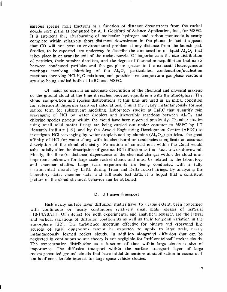
gaseous species mole fractions as a function of distance downstream from the rocket nozzle exit. plane as computed by A. I. Goldford of Science Application, Inc., for MSFC. It is apparent that afterburning of molecular hydrogen and carbon monoxide is nearly complete within relatively short distances downstream in the plume. In fact it appears that CO will not pose an environmental problem at any distance from the launch pad. Studies, to be reported, are underway to describe the condensation of liquid Alz03 that takes place in or near the exit of the rocket nozzle. Of importance is the size distribution of particles, their number densities, and the degree of thermal nonequilibrium that exists between condensed particles and the gas phase species in the exhaust. Heterogeneous reactions involving chloriding of the Al, O3 particulates, condensation/nucleation reactions involving HC1-H20 mixtures, and possible low temperature gas phase reactions are also being studied both at LaRC and MSFC.

Of major concern is an adequate description of the chemical and physical makeup of the ground cloud at the time it reaches buoyant equilibrium with the atmosphere. The cloud composition and species distributions at this time are used as an initial condition for subsequent dispersive transport calculations. This is the nearly instantaneously formed source term for subsequent modeling. Laboratory studies at LaRC that quantify rain scavenging of HC1 by water droplets and irreversible reactions between A120, and chlorine species present within the cloud have been reported previously. Chamber studies using small solid motor firings are being carried out under contract to MSFC by IIT Research Institute [ 191 and by the Arnold Engineering Development Center (AEDC) to investigate HCl scavenging by water droplets and by alumina (A120,)particles. The great affinity of HQ for water along with its chemisorbtion tendencies complicate an accurate description of the cloud chemistry. Formation of an acid mist within the cloud would substantially alter the description of gaseous HCl diffusion as the cloud travels downwind. Finally, the time (or distance) dependence of the chemical changes within the cloud is an important unknown for large scale rocket clouds and must be related to the laboratory and chamber studies. Large scale experiments are being conducted with a fully instrumented aircraft by LaRC during Titan and Delta rocket firings. By analyzing the laboratory data, chamber data, and full scale test data, it is hoped that a consistent picture of the cloud chemical behavior can be obtained.

D. Diffusive Transport

Historically surface layer diffusion studies have, t o a large extent, been concerned with continuous or nearly continuous relatively small scale releases of material [ 10-14,20,21]. Of interest for both experimental and analytical research are the lateral and vertical variations of diffusion coefficients as well as their temporal variation in the atmosphere [22] . The turbulence spectrum effective for plumes and crosswind line sources of small dimensions cannot be expected to apply to large scale, nearly instantaneously formed rocket clouds. In addition alongwind diffusion that can be neglected in continuous source theory is not negligible for “self-contained” rocket clouds. The concentration distribution as a function of time within large clouds is also of importance. The diffusive transport within the surface transport layer of large rocket-generated ground clouds that have initial dimensions at stabilization in excess of 1 km is of considerable interest for large space vehicle studies.

7

Ideally the problem would be solved by an initial value integration of the primitive equations, that is, the time-dependent conservation equations (mass, momentum, and energy), coupled with the turbulent diffusion equation. The wind field and temperature field would be calculated in a consistent, concurrent manner along with ground level air quality concentrations. Numerical solutions to such a problem are being sought by a variety of techniques [23-281 and could be of real value in parametric studies. These solutions basically use a primitive model that has no simplifying assumption or a diagnostic model that utilizes simplifying empirical assumptions. The analytical solutions reported in Reference 24 should also be noted. The primary problem with these primitive models is that they require large computers (250 K to 750 K words of core) and relatively long blocks of computer time (30 to 60.min).

Several practicaI considerations limited NASA’s decision to attempt such a method of solution. At the outset of the aerospace environmental studies, operational numerical techniques capable of application to the problem were not available. The requirement for carrying out real-time (rocket launch countdown time) air quality forecasting necessitated the use of a diffusion model that did not require large core storage or run time on available computers at KSC. That is, the model had to be operational on a minicomputer such as the Rocket Exhaust Effluent Diffusion Analysis (REEDA) system. Diffusion model forecasts would be needed on almost an hourly basis prior to launch for the anticipated rocket exhaust effluent monitoring program for both Titan and Space Shuttle launches. The time lag between release of meteorological sounding instrumentation and actual diffusion model forecasts makes the model run time a critical consideration.

The most widely used dispersion relations are those developed from integration of the diffusion equations from gradient transport theory. By use of simplifying assumptions and specific boundary conditions, these equations yield the Gaussian dispersion relations that are extensively documented in References 3, 4, 10, and 13. Thus, Gaussian plume theory coupled with wind field statistics from a diagnostic model, for example, should provide closed form solutions for effluent concentrations and dosages as functions of distance from an initial source location. The initial and boundary conditions appropriate to a mathematical description of the rocket ground cloud are formulated in a straightforward manner; however, obtaining values for actual modeling of a particular vehicle represents a monumental task in itself. The basic requirements necessary for modeling rocket clouds are listed in eight separate categories as follows:

1. Measured or modeled lateral wind field statistical properties.

2. Measured vertical profiles of wind speed, direction, temperature, pressure, and humidity.

3. Specification of transport layer height.

8

4. Rocket source terms:

a. Exhaust mass in cloud

b. Chemical composition

c. Chemical species distributions

d. Species partitioning between gas and condensed phases

e. Effective heat release from rocket motor and plume afterburning.

5 . Near field cloud rise and entrainment theory.

6. Cloud growth mechanism.

7. Scavenging and particulate settling expressions.

8. Ground absorption relations.

The details of a model incorporating these requirements are presented in Section 111.

1 1 1 . MODELING OF THE PHYSICAL PROCESSES ASSOCIATED WITH THE TRANSPORT OF ROCKET EXHAUST EFFLUENTS

IN THE TROPOSPHERE

Four primary factors are drivers in air quality predictions for the transport of rocket exhaust effluents in the troposphere, namely, the meteorology, the chemistry, the diffusion process, and the real-time predictions. The next consideration is the problems involved in modeling the first three factors in a manner that is compatible with real-time computations.

A. Overview

Before summarizing our views on the available data base for modeling of a transport process, a definition of what a model is and how it should function is in order.

A model is an abstract idealization of a process involving one or more functions designed to simplify our description of the process. Since the troposphere is characterized by a number of stochastic processes, a tropospheric model is a probabilistic idealization of a physical process. Data alone are spatially and temporally discrete, containing no information. The function of a model is to transform these data into a continuum of information. Naturally, the validity of the model determines the validity of the information.

9

I

Constraints on the model include the availability and scope of the data set, the mathematical approximation and the limits of >ohtion, and the complexity of analysis and data reduction that can be tolerated. In these considerations, we are interested in meteorological and chemical models that will act in support of the diffusion model to provide a viable description of the transport of rocket exhaust effluents in the troposphere. In addition, we would like to utilize the diffusion model for both climatological assessments and real-time launch air quality and surface loading predictions.

This section primarily considers the realistic parametric constraints on the modeling of the meteorology, the chemistry, and the diffusion process for a description of the rocket exhaust effluent transport process so that we can obtain a transport description that would be compatible with both climatological investigations and Shuttle launch operations. The primary constraints on meteorological modeling in the troposphere are that the atmospheric transport process is a nonstationary stochastic (random) process and the soundings of the surface mixing layer are designed to acquire data for mesoscale investigations. However, the tropospheric transport of a rocket exhaust is basically a small scale process.

If we accept these atmospheric constraints, only a bulk model for the chemistry is needed to address the chemical kinetics. Such a model can be obtained if the chemical kinetics are divided into basically a thermodynamic mode and a kinematic mode. This bimodal model for the rocket exhaust chemistry not only facilitates our description of the chemistry, but also affords the maximum freedom in modeling the bulk diffusion process within the limits of our knowledge of the governing atmospheric parameters.

Two primary techniques to model the turbulent diffusion process are fashionable. We have selected the gradient transport technique rather than the statistical technique, which means that we must obtain a solution to the nonlinear diffusion equation. Numeric and analytic solutions are available for this equation. The numeric solutions using a primitive model, like those used in the Livermore model, have required approximately 30 min to 1 h of computer time on a machine with a core of 250 K to 500 K words to obtain a diffusion prediction and are stongly dependent on a.good small to microscale meteorological model. Therefore, this does not appear to be a currently viable operational model for launch operational support. However, if the primitive model is simplified using empiricism and restricted to only predicting the. wind fields in a diagnostic model to support the diffusion prediction obtained from the gradient transport theory, a numeric solution becomes viable. Hence, we utilize the bimodal chemical model to linearize our diffusion equation and obtain an analytical solution using the separation of variables. To evaluate the resulting turbulent diffusion constants, we selected the Cramer diffusion coefficients [3,4] because they are compatible with atmospheric measurements obtained at test and launch sites and lend themselves to automated solutions. Such a model can be readily evaluated on a mini-digital-computer in less than 1 min.

This then, is essentially the logic behind the selection of the models for the NASA/MSFC Rocket Exhaust Effluent Diffusion (REED) description.

10

B. Meteorological Modeling

The modeling of the atmospheric kinetics and thermodynamic parameters is probably the most important single model in the development of an accurate tropospheric transport description for rocket exhaust effluents. To understand the complexities of atmospheric modeling, it is necessary to first inventory the types and sources of meteorological data that are available.

At KSC and Vandenberg Air Force Base (VAFB), there are networks of towers that provide a continuous temporal history of the horizontal wind kinematics, the humidity profiles, and the temperature profiles for approximately the first 100 m of the atmosphere over the confines of these installations. The surface barometric pressure is also available at the weather stations. Other variables such as the surface density and virtual temperature are calculated using the standard thermodynamic models [29-3 2 1.

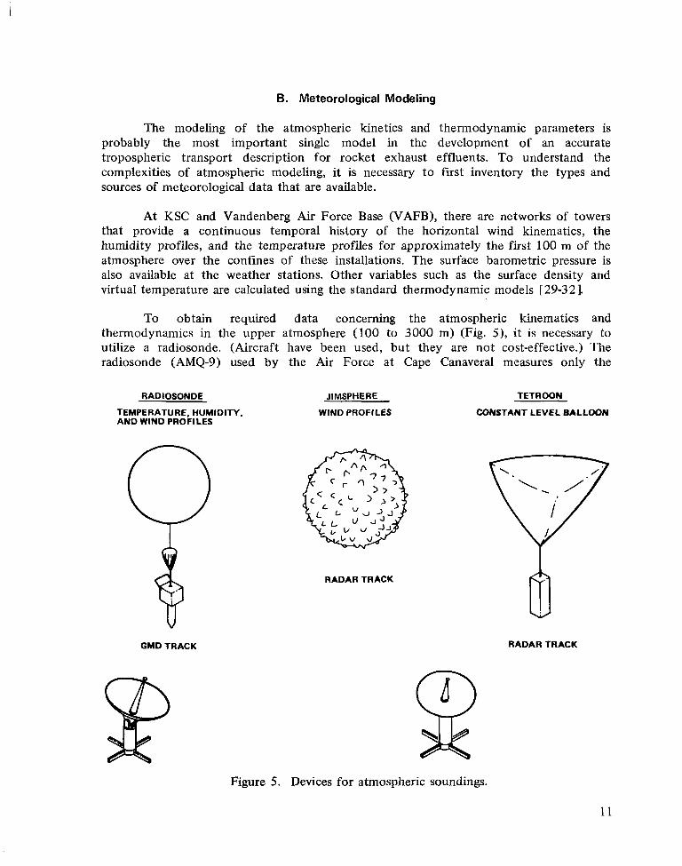
To obtain required data concerning the atmospheric kinematics and thermodynamics in the upper atmosphere (100 to 3000 m) (Fig. 5), it is necessary to utilize a radiosonde. (Aircraft have been used, but they are not cost-effective.) The radiosonde (AMQ-9) used by the Air Force at Cape Canaveral measures only the

RADIOSONDE JIMSPHERE TETROON

TEMPERATURE, HUMIDITY, WIND PROFILES CONSTANT LEVEL BALLOON AND WIND PROFILES

RADAR TRACK

GMD TRACK RADAR TRACK

Figure 5. Devices for atmospheric soundings.

11

temperature and humidity - not pressure - as it ascends through the atmosphere [32]. The rawinsonde telemetry system is utilized to determine the wind velocity as a function of altitude. Under normal operations there is currently only one radiosonde sounding made per day; however, i t is feasible during launch operations to obtain a sounding approximately every hour. More accurate kinematic information can be obtained using a Jimsphere sounding because of its improved aerodynamics. During launch operations for the NASA Titan Exhaust Effluent Prediction and Monitoring Program, a Jimsphere and a rawinsonde sounding are alternately released each hour during the 14 h period prior to launch [33]. The time duration over which these measurements are made in an atmospheric layer is relatively short (a matter of minutes - rise rate is about 5 m/s). Information on the pressures and densities aloft are obtained using standard thermodynamic relations with rawinsonde measurements; that is, they are not the result of a direct measurement [32].

Other sounding devices include windsondes, tetroons, and tetroonsondes [341 . The windsonde provides the same information as a Jimsphere - wind kinematics -however, the windsonde is tracked by a GMD rather than radar like the Jimsphere. Tetroons provide Lagrangian' (spatial) information rather than the Eulerian' (point) information that the other sounding devices provide. The straight tetroon (1 m3) is tracked by a radar and provides only temporal and spatial wind kinematics for a selected altitude. It was found that the interpretation of the data was sometime impossible. For example, when a sudden change in altitude occurred, was the change due to a vertical wind or was it due to a change in density? Hence, we introduced the tetroonsonde - a large tetroon (6 m3) with a radiosonde - to retrieve Lagrangian kinematic and thermodynamic information with a GMD.

The primary point of this review of the information retrieved from normal meteorological soundings of the atmosphere is to emphasize how limited our data base is for the surface mixing layer in the atmosphere. Because of the stochastic nature of the atmosphere, modeling of local atmospheric conditions aloft based on surface measurements of the kinematics and thermodynamics is very crude and is not generally reliable enough for a highly sophisticated transport model.

The validity of a vertical sounding as representative of the local conditions assumes that the local horizontal meteorological parameters are homogeneous and ergodic (statistically stationary), Le., that the Eulerian information is Lagrangian. The utilization of a sounding for this type of representation means the local terrain effects and land-sea interfaces must be neglected. For synoptic meteorological work where the interest is in large scale (thousands of kilometers) and mesoscale (tens to a few hundred kilometers) frontal. systems, these soundings along with the associated first-order assumptions are serviceable. However, in the transport modeling of the diffusion process, the scales of interest are small - similar to those associated with thunderstorms and tornadoes. Thus, the precision in the predictions for the transit path and concentration field associated with the rocket exhaust effluents is subject to constraints similar to those in the prediction for thunderstorms and tornadoes. The measurements aloft are being made over

1. This is the normal assumption associated with these measurements; however, it should be recognized that this is an approximation.

12

- . . . - .. . . ... . ..- .. . . . . - ... ..... I

intervals that are less than the coherency time for atmospheric stochastic process [35]. This means that the thermodynamic and kinematic parameters do not necessarily represent an ensemble average. The validity of the sounding to represent an ensemble average is directly proportional to the size of the scale of the process being modeled. In small scale processes, the local variation of these atmospheric parameters is large compared to the mesoscale processes (or large scale processes), where these variations tend to be relatively small because of spatial averaging. Hence, the normal meteorological model is designed to interface with medium or large scale models (that is, a bulk model), which tend to suppress local variations in the thermodynamic and kinematic parameters.

To some degree, terrain effects and land-sea interfaces can be overcome by the use of a tetroonsonde (constant level balloon). This is especially true for a transport model of a discrete source such as a rocket exhaust cloud. It may well be that the tetroonsonde could be the most important single tool in obtaining a spatial description of the horizontal kinematic and turbulent intensities. However, a model is needed to determine the most representative altitude to fly tetroons in order to obtain a representative transport description for the surface transport layer. In addition, this illustrates the need for a diagnostic mesoscale transport model to support the atmospheric data analysis.

There are still other measurement techniques for determining atmospheric kinematics and thermodynamics for the surface mixing layer, but consideration of these will be omitted here because they are either research techniques that have not been adequately validated or they are not cost-effective. In general then, detailed information is not available on an operational basis to establish small scale operational models for the atmosphere at the present time.

C. Modeling of the Rocket Exhaust Effluent Chemistry

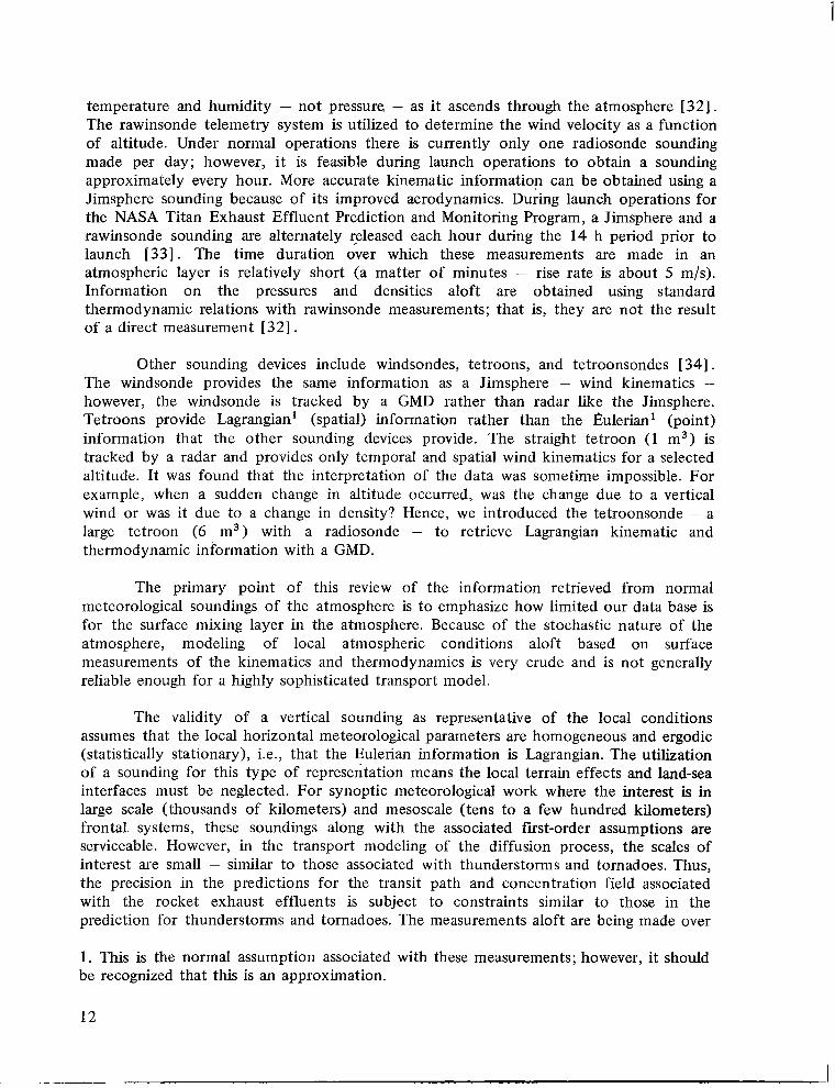
The chemical models relevant to the production and transport of rocket exhaust effluents will be considered (Fig. 6). The objective is to isolate the chemical processes into models that can be interfaced with meteorological and diffusion models to provide an accurate transport description of the concentration field of the exhaust constituent for air quality and environment assessments. These assessments are required to support both mission planning activities and launch operations. An additional constraint is imposed in the support of launch operations, namely, the requirement for real-time predictions that account for the nonstationary nature of the troposphere.

The complexities of the rocket exhaust chemical kinetics (and area transport models) can be greatly simplified by dividing the transport process into the initial thermodynamic mode and then the kinematic mode. The thermodynamic mode (which naturally includes some kinematics) shall be considered to include the chemistry oocurring prior to the exhaust cloud reaching buoyant equilibrium with the atmosphere, that is, cloud stabilization. The kinematic mode is the chemical phase after cloud

13

THERMODYNAMIC MODE CLOUD RISE

I

SOURCE DEFINITION

1. AMOUNT OF EFFLUENTS 2. AMOUNT OF HEAT RELEASED 3. PARTITIONING OF EFFLUENTS

II PRIMARY EFFLUENTS OF INTEREST

KINEMATIC MODEL

I

DIFFUSION KINETIC

1. PARTITIONING RATES 2. PRECIPITATION SCAVENGING 3. ACID MIST FORMATION

1

HYDROGEN CHLORIDE (HCI) - A I R QUALITY ALUMINA (A12031 - A I R QUALITY CARBON MONOXIDE (CO) - AFTERBURNING WATER VAPOR (H20) - A C I D FORMATION

I

Figure 6 . Bimodal rocket exhaust effluent chemistry.

stabilization (thermodynamic equilibrium). The selection of the stabilization of the exhaust cloud as the point of division between chemical processes is done strictly to facilitate the transport description; however, it does tend to mark the termination of many thermodynamic chemical processes and the start of new chemical processes.

Again, in the interest of simplification, we establish the basic spatial region of interest and chemical knowledge required during each chemical mode that is relevant to the rocket exhaust effluent transport description. Because the primary objective of this work is in support of tropospheric air quality, surface loading effects, and environmental assessments, we can basically restrict our scope of investigation to the surface mixing layer of the atmosphere (surface 500 to 2000 m). The effluents in the exhaust plume that are trapped in the surface transport layer are defined to be in the exhaust ground cloud, since only they tend to interact with the surface. The heat released and the chemical composition - especially the amount and partitioning of HC1 and Al,O, - at cloud stabilization are primary chemical data points needed from the thermodynamic model and are used in the cloud rise model. The primary chemical kinetics needed during the kinematic phase for the diffusion model are the rate coefficients for the partitioning, surface depletion, precipitation scavenging, acid rainout, and alumina fallout.

More specifically, in the thermodynamic mode the heat release by the rocket exhaust is essential in our cloud rise model for determination of the cloud stabilization height for the exhaust effluent. Our investigation suggests that the models for single phase flow (gas phase) do not afford realistic qualities for the amount of heat release [ 3 6 ] . The two phase models (gas and solid) currently appear to be the more realistic approach in determining the heat release. The question of afterburning is also an important consideration in terms of both the heat release and the inventory of the amount of CO and COz present at cloud stabilization. Radiation energy losses are also important [ 3 7 ] .

14

Other factors currently under investigation include the effects of plume impingement and the cooling water in the flame trench and on the launch tower on both the constituent inventory of the exhaust cloud at stabilization and the amount of heat lost from the vaporization of this cooling water. The effect of atmospheric conditions, such as relative humidity, on the chemistry during the thermodynamic phase is another problem that will require consideration.

The constituent inventory at the end of the thermodynamic phase becomes the source chemistry or boundary conditions for the kinematic phase. Currently, two major families of uncertainty exist. The carbon monoxide and carbon dioxide balance, which is a function of the afterburning, is not well known. Propulsion computer programs exist that should afford additional enlightenment in this area; however, this is not a real problem area in air quality estimates since our worst case assessment does not indicate a potential air quality problem. The other major family of constituents, hydrogen chloride, water, and alumina, is a potential problem that does not lerd itself to a simple solution. In the initial part of the thermodynamic phase, the F . ,h temperatures suppress the interaction of these constituents by maintaining them in the water and hydrogen chloride vapor phase. However, by the time the exhaust cloud reaches stabilization, the chemical reaction between the HC1/H2O/Alz0, has started. For example, the HCl/Hz 0 interaction in the exhaust cloud can result in the formation of an acid mist that can result in an acid rain under the proper thermodynamic conditions. (This is similar to the formation of raindrops in. a cloud.) Rain passing through the exhaust cloud can result in the precipitation scavenging of the hydrogen chloride. The HC1/A12O3 interaction can result in a general depletion of the hydrogen chloride. If the kinetics of the chemical reactions are neglected, our primary effect is to overestimate the source strength of the exhaust constituents. This means that higher concentrations will be predicted than actually exist - resulting in unnecessarily restrictive launch constraints.

In the kinematic transport phase, there is still a need for a model describing the chemical reactions and their kinetics in terms of the atmospheric parameters. In addition to the HC1/H20/Al, 0, interactions like the formation of acid mist, precipitation scavenging, and rainout that were just considered, the surface chemistry must now be considered for Earth quality assessments; for example, the surface absorption of the hydrogen chloride for land surfaces and water surfaces along with the reflection coefficient of the alumina in terms of its size spectrum.

While not all of the rocket exhaust chemistry has been discussed, hopefully, the salient features that have been touched upon clearly illustrate the need for chemical models for both the thermodynamic and kinematic transport modes of rocket exhaust effluents. While laboratory, chamber, and field tests have afforded some insight into rocket exhaust chemistry and techniques for modeling the chemistry, much remains to be learned in this area. The general approach to the modeling rocket exhaust effluent chemistry currently being employed as a consequence of the limited state of the art knowledge is to overestimate the potential effects to ensure safe operations.

15

SEPARATION

VARIABLES

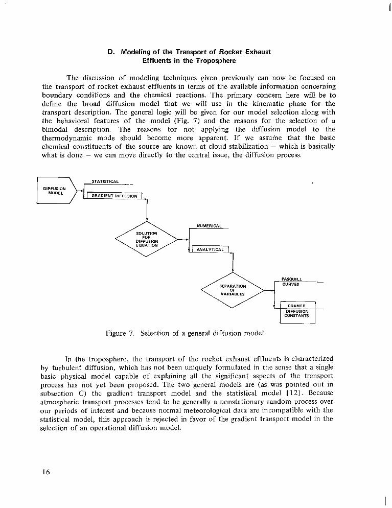
D. Modeling of the Transport of Rocket Exhaust Effluents in the Troposphere

The discussion of modeling techniques given previously can now be focused on the transport of rocket exhaust effluents in terms of the available information concerning boundary conditions and the chemical reactions. The primary concern here will be to define the broad diffusion model that we will use in the kinematic phase for the transport description. The general logic will be given for our model selection along with the behavioral features of the model (Fig. 7) and the reasons for the selection of a bimodal description. The reasons for not applying the diffusion model to the thermodynamic mode should become more apparent. If we assume that the basic chemical constituents of the source are known at cloud stabilization - which is basically what is done - we can move directly to the central issue, the diffusion process.

\ STATISTICAL

L I NUMERICAL

SOLUTION

DIFFUSION EOUATION

SEPARATION

VARIABLES

CRAMER

CONSTANTS

Figure 7. Selection of a general diffusion model.

In the troposphere, the transport of the rocket exhaust effluents is characterized by turbulent diffusion, which has not been uniquely formulated in the sense that a single basic physical model capable of explaining all the significant aspects of the transport process has not yet been proposed. The two general modeli are (as was pointed out in subsection C) the gradient transport model and the statistical model [ 121. Because atmospheric transport processes tend to be generally a nonstationary random process over our periods of interest and because normal meteorological data'are incompatible with the statistical model, this approach is rejected in favor of the gradient transport model in the selection of an operational diffusion model.

16

I

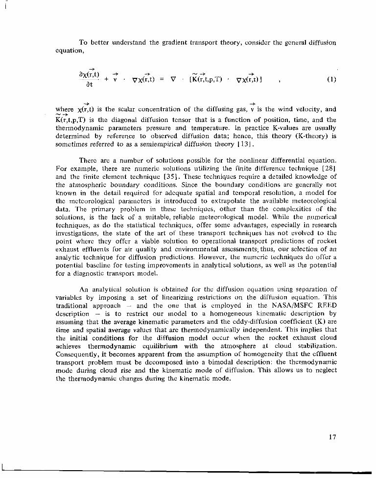
To better understand the gradient transport theory, consider the general diffusion equation,

+ + where X(r,t) is the scalar concentration of the diffusing gas, v is the wind velocity, and - 3

K(r,t,p,T) is the diagonal diffusion tensor that is a function of position, time, and the thermodynamic parameters pressure and temperature. In practice K-values are usually determined by reference to observed diffusion data; hence, this theory (K-theory) is sometimes referred to as a semiempirical diffusion theory [ 131 .

There are a number of solutions possible for the nonlinear differential equation. For example, there are numeric solutions utilizing the finite difference technique [281 and the finite element technique [ 351. These techniques require a detailed knowledge of the atmospheric boundary conditions. Since the boundary conditions are generally not known in the detail required for adequate spatial and temporal resolution, a model for the meteorological parameters is introduced to extrapolate the available meteorological data. The primary problem in these techniques, other than the complexities of the solutions, is the lack of a suitable, reliable meteorological model. While the numerical techniques, as do the statistical techniques, offer some advantages, especially in research investigations, the state of the art of these transport techniques has not evolved to the point where they offer a viable solution to operational transport predictions of rocket exhaust effluents for air quality and environmental assessments; thus, our selection of an analytic technique for diffusion predictions. However, the numeric techniques do offer a potential baseline for testing improvements in analytical solutions, as well as the potential for a diagnostic transport model.

An analytical solution is obtained for the diffusion equation using separation of variables by imposing a set of linearizing restrictions on the diffusion equation. This traditional approach - and the one that is employed in the NASA/MSFC REED description - is to restrict our model to a homogeneous kinematic description by assuming that the average kinematic parameters and the eddy-diffusion coefficient (K) are time and spatial average values that are thermodynamically independent. This implies that the initial conditions for the diffusion model occur when the rocket exhaust cloud achieves thermodynamic equilibrium with the atmosphere at cloud stabilization. Consequently, it becomes apparent from the assumption of homogeneity that the effluent transport problem must be decomposed into a bimodal description: the thermodynamic mode during cloud rise and the kinematic mode of diffusion. This allows us to neglect the thermodynamic changes during the kinematic mode.

17

L

,. ,. . ... ....-,.. .,.. ,.. _. . .._.... - . ..- ... ........ ,, . ... - _.. _.. , ., ., ,

From the standpoint of meteorological and chemical modeling, we have also obtained a viable position since the utilization -of the parameters from these two models will be in terms of average values which suppress most of the uncertainties in the microphysics and chemistry. The thermodynamic and kinematic profiles obtained from a rawinsonde sounding are valid ensemble averages that are representative of the general local conditions. In the case of the chemistry, we c'an generally neglect the microchemistry since fluctuations in it are basically averaged out and the chemical model is only required to represent the average process. (One exception could be the formation of the acid mist.) Thus, averaging the input parameters to the diffusion model permits us to both utilize more existing measuring techniques and models for the atmospheric parameters and chemical processes - yet still take advantage of new improvements as they are developed.

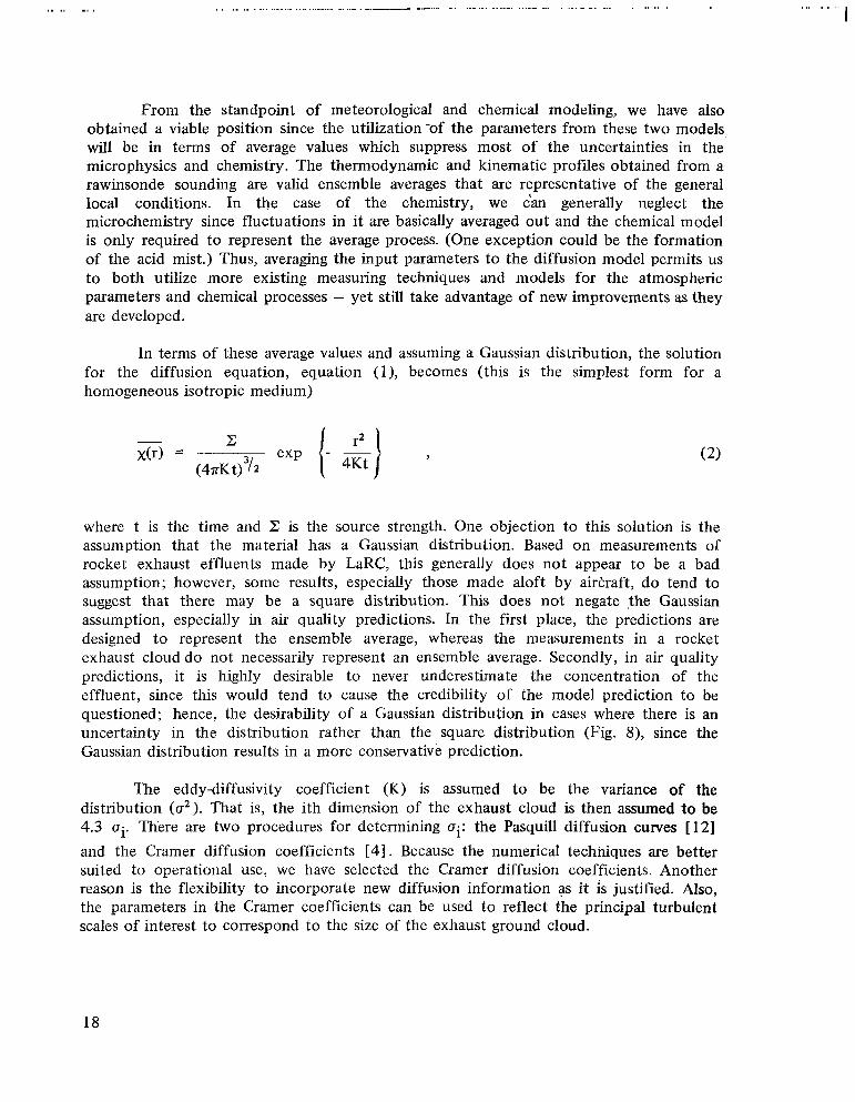
In terms of these average values and assuming a Gaussian distribution, the solution for the diffusion equation, equation ( l ) , becomes (this is the simplest form for a homogeneous isotropic medium)

where t is the time and 2 is the source strength. One objection to this solution is the assumption that the material has a Gaussian distribution. Based on measurements of rocket exhaust effluents made by LaRC, this generally does not appear to be a bad assumption; however, some results, especially those made aloft by airtraft, do tend to suggest that there may be a square distribution. This does not negate ,the Gaussian assumption, especially in air quality predictions. In the first place, the predictions are designed to represent the ensemble average, whereas the measurements in a rocket exhaust cloud do not necessarily represent an ensemble average. Secondly, in air quality predictions, it is highly desirable to never underestimate the concentration of the effluent, since this would tend to cause the credibility of the model prediction to be questioned; hence, the desirability of a Gaussian distribution in cases where there is an uncertainty in the distribution rather than the square distribution (Fig. S ) , since the Gaussian distribution results in a more conservative prediction.

The eddy-diffusivity coefficient (K) is assumed to be the variance of the distribution (a'). That is, the ith dimension of the exhaust cloud is then assumed to be 4.3 ai. T�iere are two procedures for determining ai: the Pasquill diffusion curves [ 121 and the Cramer diffusion coefficients [4] . Because the numerical techniques are better suited to operational use, we have selected the Cramer diffusion coefficients. Another reason is the flexibility to incorporate new diffusion information as it is justified. Also, the parameters in the Cramer coefficients can be used to reflect the principal turbulent scales of interest to correspond to the size of the exhaust ground cloud.

18

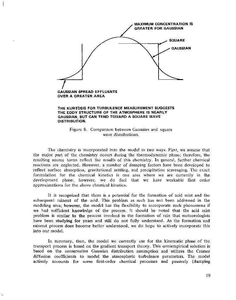
/ MAXIMUM CONCENTRATION IS GREATER FOR GAUSSIAN

GAUSSIAN SPREAD EFFLUENTS OVER A GREATER AREA

THE KURTOSIS FOR TURBULENCE MEASUREMENT SUGGESTS THE EDDY STRUCTURE OF THE ATMOSPHERE IS NEARLY GAUSSIAN, BUT CAN TEND TOWARD A SQUARE WAVE DISTRIBUTION.

Figure 8. Comparison between Gaussian and square wave distributions.

The chemistry is incorporated into the model in two ways. First, we assume that the major part of the chemistry occurs during the thermodynamic phase; therefore, the resulting source terms reflect the results of this chemistry. In general, further chemical reactions are neglected. However, a number of damping factors have been developed to reflect surface absorption, gravitational settling, and precipitation scavenging. The exact formulation for the chemical kinetics is one area where we are currently in the development phase; however, we do feel that we have workable first order approximations for the above chemical kinetics.

It is recognized that there is a potential for the formation of acid mist and the subsequent rainout of the acid. This problem as such has not been addressed in the modeling area; however, the model has the flexibility to incorporate such phenomena if we had sufficient knowledge of the process., It should be noted that the acid mist problem is similar to the process involved in the formation of rain that meteorologists have been studying for years and still do not fully understand. As the formation and rainout process does become better understood, we do hope to actively incorporate this into our model.

In summary, then, the model we currently use for the kinematic phase of the transport process is based on the gradient transport theory. This semiempirical solution is based on the conservative Gaussian distribution assumption and utilizes the Cramer diffusion coefficients to model the atmospheric turbulence parameters. The model actively accounts for some first-order chemical processes and passively (damping

19

coefficient) accounts for others. The results of this diffusion description are ensemble averages and may not always reflect the instantaneous (less than the atmospheric coherency time) local values commonly measured in the near field [35,38,39].

Since the transport process is dominated by the kinematic phase, careful consideration of thermodynamics is reserved for the next section.

E. Applications

There are three primary applications for the rocket exhaust effluent transport predictions obtained with the NASA/MSFC REED description. The description is used in air quality and environmental assessments for:

0 Mission planning acitivities and environmental assessments.

0 Prelaunch forecasts of the environmental effects of launch operations.

0 Postlaunch environmental analysis.

Each of the above applications imposes different modeling requirements that will be considered as a prologue to our discussion of the REED description.

Presently the primary requirement for the REED description is in the preparation of environmental assessments and in examining the potential for operational environmental constraints. Both of these functions require a climatological assessment for atmospheric conditions using the meteorological model in the REED description. This means that large numbers of carefully selected rawinsonde soundings must be used as inputs to the diffusion model to obtain the statistical base in these climatological environment assessments. Hence, we want a simple, reliable model with a minimum of fine structure that will address only the central question. One reason for this simplistic approach is that the fine structure of the diffusion prediction will be averaged out in the volume of data being employed. Another reason is that too much fine structure would suppress some of the more essential features in the analysis and make the interpretation of results too complex. Yet another consideration for a simplistic approach is that the data reduction procedures must be automated to the greatest possible degree and the computation time must be reduced to a minimum to keep the assessments cost-effective. (A complete climatological air quality assessment for KSC would require a considerable amount. of computer time.)

In the second application of diffusion predictions, forecasting the transport of rocket exhaust effluents in advance of a launch, we are limited primarily by the dynamic variability of the atmospheric conditions. In general, the limited accuracy of the forecasted atmospheric parameters does not warrant a sophisticated diffusion prediction when the atmospheric conditions are straightforward. However, the speed and reliability of the diffusion calculation are extremely important. For this reason a real-time diffusion

20

i

analysis system such as the NASA/MSFC REEDA system is important; that is, it is very desirable to have a small computer at the launch site to make real-time diffusion predictions for both the use of launch operation personnel and, for the deployment of an exhaust monitoring network. This means that the diffusion calculations must be simple enough to be placed on a small portable computer (32K words) and run in less than 10 min. Ideally, the on-line real-time diffusion system should be interactive so that the forecaster and the users can quickly test the results of a small perturbation in atmospheric parameters. or call for specific information that they may desire.

In the third application of diffusion predictions, postlaunch analysis of the transport of the rocket exhaust effluents, detailed computations of the diffusion process are usually required. Because we normally will have at least a rawinsonde sounding of the atmosphere at launch time, this type of detailed analysis is justified in terms of our atmospheric data. In general, then, a more exact diffusion model is appropriate for postlaunch analysis than is necessary for either climatological investigations or for forecasting environmental effects. This diffusion model must, however, be of the same form as the other diffusion models to maintain continuity.

A great deal of experience has been obtained at actual Titan launches and is reflected in the evolution of the REED description in Section IV. It should be recognized that while the central core of the diffusion model is well defined, the peripheral aspects of this model are still soft. These peripheral aspects are still somewhat dependent on the future applications that may evolve and on the state of the art of atmospheric soundings and models.

IV. NASA/MSFC ROCKET EXHAUST EFFLUENT DIF FUSION (REED) DESCRIPTION

The spatial description, in terms of concentration and dosage, of the dispersive transport of effluents from a discrete source is afforded by the NASAlMSFC REED description. This description, which represents an update in our technology and techniques, is composed of three models: the Meteorological Model, the rocket exhaust Cloud Rise Model, and the Multilayer Diffusion Model. The techniques and options for these models are discussed herein. All models here have been updated [4]recently, and many of the algorithms that are given here cannot be found in earlier literature [ 3 ] .

In this section, an overview of the REED description is provided in the first subsection followed by discussions of the cloud rise model, the multilayer diffusion model, and real-time diffusion predictions. Since our current meteorological model utilizes only the normal forecast models and the mesoscale model is currently being developed, this model will not be considered here.

21

A. Overview of the NASA/MSFC REED Description

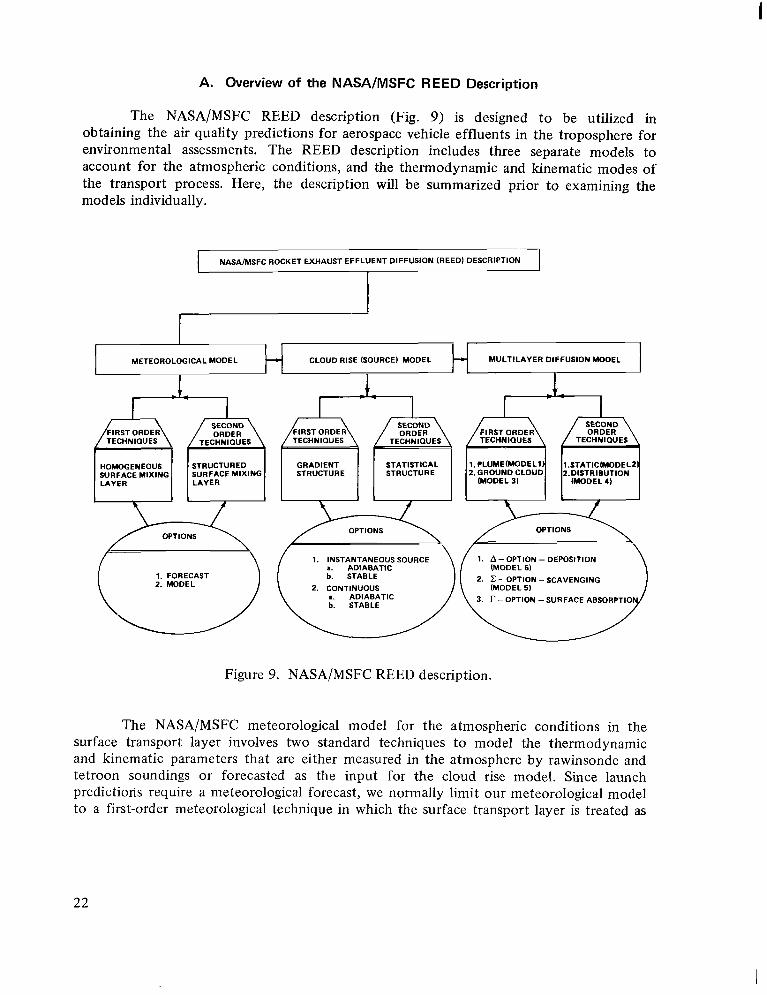
The NASA/MSFC REED description (Fig. 9) is designed to be utilized in obtaining the air quality predictions for aerospace vehicle effluents in the troposphere for environmental assessments. The REED description includes three separate models to account for the atmospheric conditions, and the thermodynamic and kinematic modes of the transport process. Here, the description will be summarized prior to examining the models individually.

NASA/MSFC ROCKET EXHAUST EFFLUENT DIFFUSION (REED) DESCRIPTION

SURFACE

METEOROLOGICAL MODEL CLOUD RISE (SOURCE) MODEL MULTILAYER DIFFUSION MODEL

I I I

r-l II ORDER

TECHNIOUES TECHNIOUES TECHNIOUES TECHNIQUES

HOMOGENEOUS STRUCTURED GRADIENT STATISTICAL l.CLUME(MODEL1 l.STATIC(MODEL2 2.DISTRIBUTIONMIXING I SURFACE MIXING STRUCTURE STRUCTURE 12.GROUND CLOUD1 1 (MODEL41 1LAYER ILAYER (MODEL3)

OPTIONSOPTIONS = 1. INSTANTANEOUS SOURCE 1. A -OPTION - DEPOSITION

a. ADIABATIC (MODEL 6)?J1. FORECAST 2. CONTINUOUS (MODEL 5 )

b. STABLE 2. -OPTION - SCAVENGING

a. ADIABATIC b. STABLE /i 3. r -OPTION -SURFACE ABSORPTIO 3

Figure 9. NASA/MSFC REED description.

The NASA/MSFC meteorological model for the atmospheric conditions in the surface transport layer involves two standard techniques to model the thermodynamic and kinematic parameters that are either measured in the atmosphere by rawinsonde and tetroon soundings or forecasted as the input for the cloud rise model. Since launch predictions require a meteorological forecast, we normally limit our meteorological model to a first-order meteorological technique in which the surface transport layer is treated as

22

a homogeneous layer. This same first-order meteorological technique is also used in climatological environmental assessments. In postlaunch analysis, a second-order meteorological technique is utilized, where the surface transport layer is structured into a number of more nearly homogeneous layers. (Here the term homogeneous layer means that the layer parameters can be modeled in terms of representative mean values.) Options exist with both of these techniques to include precipitation effects and land-sea interfaces.

The NASA/MSFC Exhaust Cloud Rise Model is designed to utilize the output of the meteorological model and define the source parameters for the multilayer diffusion model. This model has a first-order gradient technique that uses two value differences to obtain thermodynamic buoyance parameters and a second-order statistical technique that uses regression analysis to obtain the thermodynamic parameters. Since these cloud rise techniques are dependent on the meteorological techniques, there is normally a direct coupling of first or second order techniques between these models. In addition, there are two options for the techniques defined by the vehicle type. There is an option for instantaneous sources for solid rockets such as the Titan 111, and the option for continuous sources is for liquid rockets such as the Saturn. In the case of vehicles such as the Delta-Thor or the Space Shuttle, a combination of options must be used that utilizes both the instantaneous and continuous source options to account for the combination of solid motors and liquid engines. Two options also exist to account for the thermodynamic lapse rate, namely, the adiabatic option and the stable option. These options are always combined with the source options.

The NASA/MSFC Multilayer Diffusion Model is designed to take the output of the exhaust cloud rise model and generate a mapping for the air quality concentration levels of the exhaust constituents. This is accomplished by using one of two techniques, the unlayered first-order technique or the layered second-order technique. The two first-order techniques are: (1) the plume technique (model 1) where a cylindrical distribution is assumed, and (2) the ground cloud technique (model 3) in which an ellipsoidal distribution in a homogeneous surface transport layer is assumed. The second-order techniques are: (1) the static plume technique (model 2) where it is assumed that there is a layer where no turbulent mixing occurs, and (2) the distribution technique (model 4) where the surface transport layer is layered into statistically thermodynamically and kinematically homogeneous layers along with a well distributed source. The multilayer diffusion model has three options that can be used with either technique. There is a precipitation scavenging option (model 5 ) , or X-option, to account for the depletion of an exhaust constituent during rain; there is a deposition option (model 6), or A-option, to account for gravitational settling; and a new option, the I?-option, has been added to account for surface absorption of a constituent. These options afford the potential for studying the Earth quality. (Here the term air quality is used to denote constituent burden in the air, whereas Earth quality is used to denote the amount of the constituent left on a surface by surface loading.) The current format of the NASA/MSFC multilayer diffusion model is for air quality investigations; however, the

23

Earth quality can be readily determined by basically binary operation of the model. For example, if the difference between dosages obtained from running the diffusion model with r-option equal to zero and to one is taken amid multiplied by the diffusion rate, we obtain the surface loading. In addition, the diffusion model has provisions for cold spills and fuel leak calculations in the surface mixing layer.

This summary of the REED description with its models, techniques, and options is a preface to consideration of the algorithms used in the techniques.

6. NASA/MSFC Rocket Exhaust Cloud Rise Model

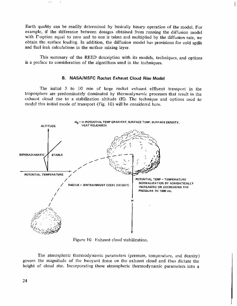
The initial 5 to 10 min of large rocket exhaust effluent transport in the troposphere are predominately dominated by thermodynamic processes that result in the exhaust cloud rise to a stabilization altitude (HI. The technique and options used .to model this initial mode of transport (Fig. 10) will be considered here.

H s = H (POTENTIAL TEMP GRADIENT, SURFACE TEMP, SURFACE DENSITY, ALTITUDE HEAT RELEASED)

I/SUPERADll

POTENTIAL TEMPERATURE / / I POTENTIAL TEMP = TEMPERATURE

NORMALIZATION BY ADIABATICALLY/ RADIUS = (ENTRAINMENT COEF) (HEIGHT) I OR THE

/ PRESSURE TO 1000 mb.

/ I/ H

/ I

Figure 10. Exhaust cloud stabilization.

The atmospheric thermodynamic parameters (pressure, temperature, and density) govern the magnitude of the buoyant force on the exhaust cloud and thus dictate the height of cloud rise. Incorporating these atmospheric thermodynamic parameters into a

24

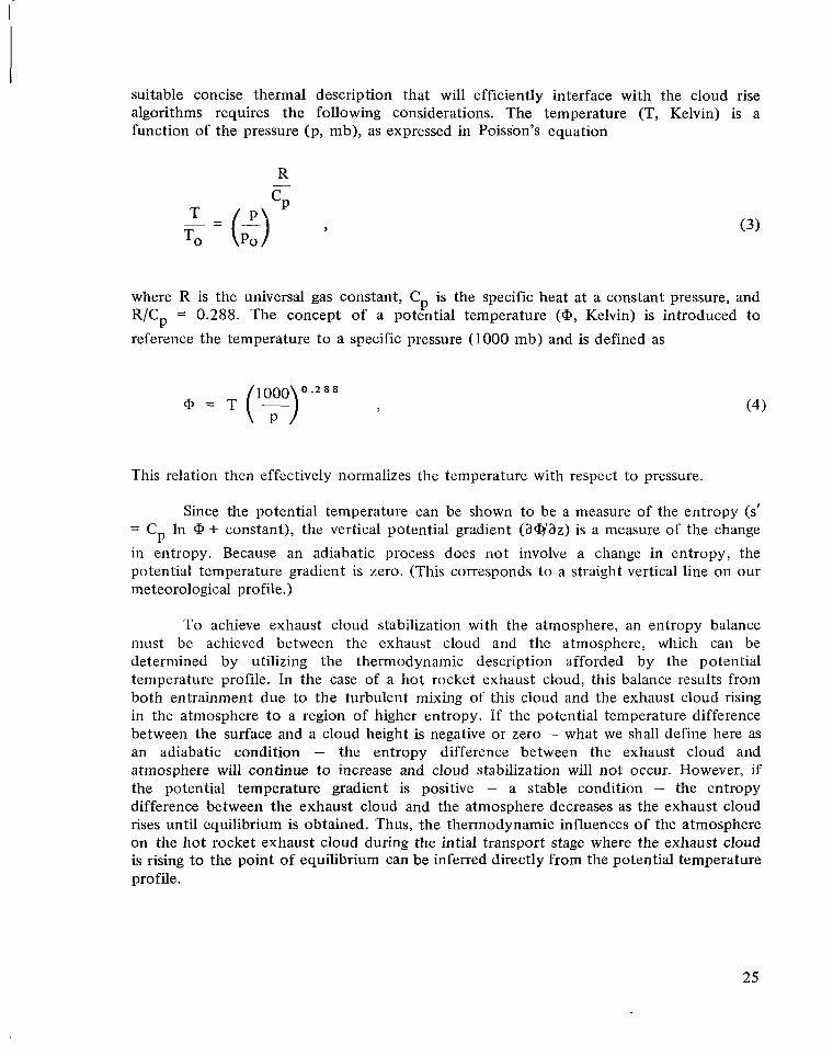
suitable concise thermal description that will efficiently interface with the cloud rise algorithms requires the following considerations. The temperature (T, Kelvin) is a function of the pressure (p, mb), as expressed in Poisson’s equation

T Y ,-=(;> (3)

TO

where R is the universal gas constant, CP is the specific heat at a constant pressure, and R/Cp = 0.288. The concept of a potential temperature (a,Kelvin) is introduced to reference the temperature to a specific pressure (1000 mb) and is defined as

a = . ( ? )1000 o - 2 8 8 , (4)

This relation then effectively normalizes the temperature with respect to pressure.

Since the potential temperature can be shown to be a measure of the entropy (s’ = CP In + constant), the vertical potential gradient ( a g a z ) is a measure of the change in entropy. Because an adiabatic process does not involve a change in entropy, the potential temperature gradient is zero. (This corresponds to a straight vertical line on our meteorological profile.)

To achieve exhaust cloud stabilization with the atmosphere, an entropy balance must be achieved between the exhaust cloud and the atmosphere, which can be determined by utilizing the thermodynamic description afforded by the potential temperature profile. In the case of a hot rocket exhaust cloud, this balance results from both entrainment due to the turbulent mixing of this cloud and the exhaust cloud rising in the atmosphere to a region of higher entropy. If the potential temperature difference between the surface and a cloud height is negative or zero - what we shall define here as an adiabatic condition - the entropy difference between the exhaust cloud and atmosphere will continue to increase and cloud stabilization will not occur. However, if the potential temperature gradient is positive - a stable condition - the entropy difference between the exhaust cloud and the atmosphere decreases as the exhaust cloud rises until equilibrium is obtained. Thus, the thermodynamic influences of the atmosphere on the hot rocket exhaust cloud during the intial transport stage where the exhaust cloud is rising to the point of equilibrium can be inferred directly from the potential temperature profile.

25

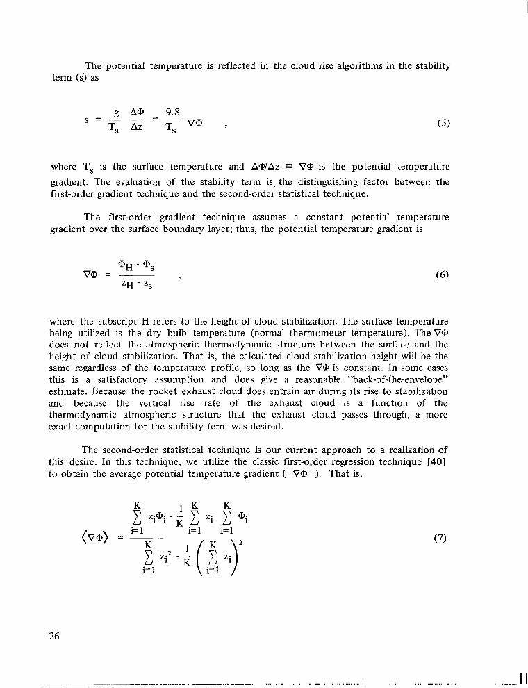
The potential temperature is reflected in the cloud rise algorithms in the stability term (s) as

A@ 9.8

where T, is the surface temperature and AWAz E V+ is the potential temperature gradient. The evaluation of the stability term is, the distinguishing factor between the first-order gradient technique and the second-order statistical technique.

The first-order gradient technique assumes a constant potential temperature gradient over the surface boundary layer; thus, the potential temperature gradient is

‘H - ‘svcp = , ‘H - ‘s

where the subscript H refers to the height of cloud stabilization. The surface temperature being utilized is the dry bulb temperature (normal thermometer temperature). The VQ, does not reflect the atmospheric thermodynamic structure between the surface and the height of cloud stabilization. That is, the calculated cloud stabilization height will be the same regardless of the temperature profile, so long as the V@ is constant. In some cases this is a satisfactory assumption and does give a reasonable “back-of-the-envelope” estimate. Because the rocket exhaust cloud does entrain air during its rise to stabilization and because the vertical rise rate of the exhaust cloud is a function of the thermodynamic atmospheric structure that the exhaust cloud passes through, a more exact computation for the stability term was desired.

The second-order statistical technique is our current approach to a realization of this desire. In this technique, we utilize the classic first-order regression technique [40] to obtain the average potential temperature gradient ( V@ ). That is,

K l K K Zi’i -

K - c zi C ‘i

i= 1 i= 1 i= 1 (7)

i=,f1 Zi)’

26

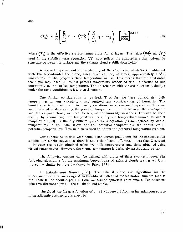
and

where (Ts) is the effective surface temperature for K layers. The values(V@) and (Ts) used in the stability term [equation (5)J now reflect the atmospheric thermodynamic structure between the surface and the exhaust cloud stabilization height.

A marked improvement in the stability of the cloud rise calculations is obtained with the second-order technique, since there can be, at times, approximately a 5°C uncertainty in the proper surface temperature to use. This means that the first-order technique may have 30 to 40 percent uncertainty associated with it because of our uncertainty in the surface temperature. The uncertainty with the second-order technique under the same conditions is less than 5 percent.

One further consideration is required. Thus far, we have utilized dry bulb temperatures in our calculations and omitted any consideration of humidity. The humidity variations will result in density variations for a constant temperature. Since we are interested in determining the point of buoyant equilibrium between the atmosphere and the exhaust cloud, we need to account for humidity variations. This can be done readily by normalizing our temperatures to a dry air temperature known as virtual temperature' [30] . If the dry bulb temperatures in equation (4) are replaced by virtual temperatures in the calculations for the potential temperatures, we obtain virtual potential temperatures. This in turn is used to obtain the potential temperature gradient.

Our experience to date with actual Titan launch predictions for the exhaust cloud stabilization height shows that there is not a significant difference - less than 2 percent - between the results obtained using dry bulb temperatures and those obtained using virtual temperatures. However, the virtual temperature is definitely aesthetically better.

The following options can be utilized with either of these two techniques. The following algorithms for the maximum buoyant rise of exhaust clouds are derived from procedures similar to those developed by Briggs I4 1I .

1. Instantaneous Source [3-51. The exhaust cloud rise algorithms for the instantaneous source are designed to be utilized with solid rocket motor launches such as the Titan I11 or Scout-Algol 111. Here we assume spherical entrainment. The solutions take two different forms - the adiabatic and stable.

The cloud rise (z) as a function of time (t) downwind from an instantaneous source in an adiabatic atmosphere is given by

27

-.. .-, ._.. . .. - . - . .. - ... ... .. .. ..

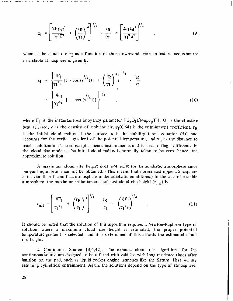
whereas the cloud rise ZI as a function of time downwind from an instantaneous source in a stable atmosphere is given by

21 = (.;I'-s(s rR~ F I '12 t)] + ($1 It4

- ­71

where FI is the instantaneous buoyancy parameter [(3gQ1)/(4?rpcpT)], QI is the effective heat released, p is the density of ambient air, q (0 .64) is the entrainment coefficient, rR is the initial cloud radius at the surface, s is the stability term [equation (5)] and accounts for the vertical gradient of the potential temperature, and xS1 is the distance to reach stabilization. The subscript I means instantaneous and is used to flag a difference in the cloud rise models. The initial cloud radius is normally taken to be zero; hence, the approximate solution.

A maximum cloud rise height does not exist for an adiabatic atmosphere since buoyant equilibrium cannot be obtained, (This means that normalized upper atmosphere is heavier than the surface atmosphere under adiabatic conditions.) In the case of a stable atmosphere, the maximum instantaneous exhaust cloud rise height ( ~ ~ 1 )is

It should be noted that the solution of this algorithm requires a Newton-Raphson type of solution where a maximum cloud rise height is estimated, the proper potential temperature gradient is selected, and it is determined if this affords the estimated cloud rise height.

2. Continuous Source [3,4,42]. The exhaust cloud rise algorithms for the continuous source are designed to be utilized with vehicles with long residence times after ignition on the pad, such as liquid rocket engine launches like the Saturn. Here we are assuming cylindrical entrainment. Again, the solutions depend on the type of atmosphere.

28

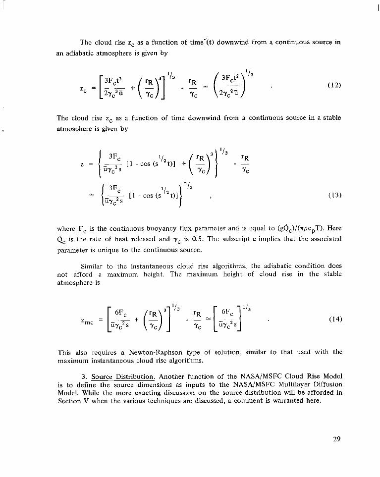
The cloud rise zc as a function of time'it) downwind from a continuous source in an adiabatic atmosphere is given by

The cloud rise zc as a function of time downwind from a continuous source in a stable atmosphere is given by

where Fc is the continuous buoyancy flux parameter and is equal to (gQc)/(rpcpT). Here Qc is the rate of heat released and yc is 0.5. The subscript c implies that the associated parameter is unique to the continuous source.

Similar to the instantaneous cloud rise algorithms, the adiabatic condition does not afford a maximum height. The maximum height of cloud rise in the stable atmosphere is

This also requires a Newton-Raphson type of solution, similar to that used with the maximum instantaneous cloud rise algorithms.

3. Source Distribution. Another function of the NASAIMSFC Cloud Rise Model is to define the source dimensions as inputs to the NASAIMSFC Multilayer Diffusion Model. While the more exacting discussion on the source distribution will be afforded in Section V when the various techniques are discussed, a comment is warranted here.

29

Within the bounds of the discussion technique being used, the modeler has the option to set the dimensions of the source in accordance with his own desires. Based on our empirical experience, the exhaust cloud radius is normally taken as the product of the entrainment coefficient times the exhaust cloud stabilization height for prelaunch predictions, where the entrainment coefficient is: (a) 0.50 for liquid rocket engines, (b) 0.64 for solid rocket motors, and (c) 0.57 for a combination of liquid and solid rockets. However, in postlaunch analysis, the actual source dimensions can be employed to obtain optimum results. In the case of the second-order distribution technique, the actual amount and size of the stabilized exhaust cloud in each layer can be utilized in postlaunch analysis.

Thus, while a general rule of thumb exists for the source dimensions of the stabilized exhaust cloud in the NASAlMSFC Cloud Rise Model, the modeler has the option to change the dimensions where more realistic values are known.

4. Summary Remarks. It is recognized that the cloud rise relations could be improved; however, these relations are presently affording reasonable results. Two primary parameters are subject to question - the entrainment coefficient and the heat released.

The entrainment coefficient (7)is defined to be the ratio of the cloud radius to the cloud centroid height. This empirical coefficient is very difficult to evaluate because of the complex exhaust cloud geometry and because it is a function of altitude. We believe that the current entrainment coefficients are almost as good as can be reasonably obtained using cloud photographs.

The amount of heat released is currently undergoing reevaluation for solid rocket motors. Earlier values were calculated based on single-phase flow and afterburning. Recent calculations [36] show that this flow must be treated as a two-phase flow - gas and particles. In addition to the afterbuming, heat losses due to radiation [43] and the pad cooling water [4] must be considered. These refinements should improve the reliability of the estimates of the heat released and thereby allow a more precise estimate of the stabilization height. (Currently we underestimate this height to prevent underestimating the maximum concentrations.) As the accuracy of these parameters improves, it should continue to reduce the potential for aerospace environmental launch constraints.

C. NASA/MSFC Multilayer Diffusion Model [4]

The NASAlMSFC Multilayer Diffusion Model is designed to provide a description of the kinematic turbulent transport of effluents released by aerospace vehicles for use in air quality and environmental assessments. The various techniques available in this model along with 'the associated assumptions will be reviewed here. Since the detailed algorithms may be beyond the interest of many readers, a general summary of the model and how it functions is presented as a preface to the algorithms.

30

1 . Modular Form of Diffusion Equation. The general differential equation for kinematic diffusion [equation ( l ) ] can be linearized by assuming that the meteorological profile represents the homogeneous average atmospheric conditions over the layer of interest and solved [equation ( 2 ) ] by separation of variables for the spatial distribution of the concentration and dosage resulting from the launch of an aerospace vehicle. A general formulation for the diffusion equation was provided previously. Definitions of the key terms are repeated here for reader convenience and a modular breakout of the diffusion equation will now be given.

Effluent Terminology

Concentration The amount of the effluent present at a specific time. The average concentration is the average amount present during the event.

Dosage The measure of the total amount of effluent (time integrated concentration) due to the launch vehicle at a specific location.

Model Terminology

Plume Cloud The cloud of rocket effluents emitted from the vehicle in flight. This cloud has a cylindrical shape whose height is defined by the vertical thickness of the layer.

Ground Cloud That cloud of rocket effluents emitted during the initial phase of vehicle launch. This cloud is assumed to have an ellipsoidal shape.

Coordinate System

Centerline The radial vector in the direction of the mean wind direction whose origin is the point of cloud stabilization. This is defined as the x-direction.

The Model

The generalized concentration model for a nearly instantaneous source is expressed as the product of seven modular terms,

Concentration = {Peak Concentration Term) X {Alongwind Term)

X {Lateral Term) X {Vertical Term)

X {Depletion Term) X {Scavenging Term)

X {Surface Absorption Term) ;

31

I

whereas the generalized dosage model for a nearly instantaneous source is defined by the produce of six modular terms,

Dosage = {Peak Dosage Terms) X {Lateral Term)

X {Vertical Term) X {Depletion Term)

X {Scavenging Term) X {Surface Absorption Term)

Thus, the mathematical description for the concentration and dosage models permits flexibility in application to various aerospace sources with an approximate ellipsoidal geometry and for changing atmospheric parameters while always maintaining a rigorous mass balance.

Two obvious differences exist between the concentration and dosage models. First, the peak concentration term refers to the concentration at the point x, y = 0, z = H (where x is the wind direction and H is any height) and is defined by the expression

tPeak Concentration = ~- - ,

where C is the mass source strength and ai is the Cramer coefficient for the standard deviation of the concentration distribution in the ith direction. The peak dosage term is given by

Peak Dosage = ~-72niiayoz

where U is the mean wind speed over the layer. The second difference between these models is that the concentration contains a modular alongwind term (x-direction) to account for downstream temporal effects not considered in the dosage model. The alongwind term affords an exponential decay in concentration as a function of cloud transit time, concentration distribution, and the mean wind speed.

The lateral term (y-direction) is another exponential decay term and is a function of the Gaussian spreading rate and the distance laterally from the mean wind azimuth. The vertical term (z-direction) is a rather complex decay function since it contains

3 2

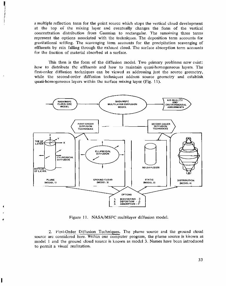
a multiple reflection term for the point source which stops the vertical cloud development at the top of the mixing layer and eventually changes the form of the vertical concentration distribution from Gaussian to rectangular. The remaining three terms represent the options associated with the techniques. The deposition term accounts for gravitational settling. The scavenging term accounts for the precipitation scavenging of effluents by rain falling through the exhaust cloud. The surface absorption term accounts for the fraction of material absorbed at a surface.

This then is the form of the diffusion model. Two primary problems now exist: how to distribute the effluents and how to maintain quasi-homogeneous layers. The first-order diffusion techniques can be viewed as addressing just the source geometry, while the second-order diffusion techniques address source geometry and establish quasi-homogeneous layers within the surface mixing layer (Fig. 11).

NASAIMSFC CLOUD RISE MULTILAYER DIFFUSION

ASSESSMENTS

I SECOND ORDER

DIFFUSION DIFFUSION TECHNIOUES TECHNIOUES

DIFFUSION

NO DIFFUSION6 PLUME GROUND CLOUD STATIC DISTRIBUTION

(MODEL 1) (MODEL 3) I (MODEL 2 ) (MODEL 41

1. SCAVENGING - Z 2. DEPOSITION - A 3. ABSORPTION -r

Figure 11 . NASA/MSFC multilayer diffusion model.

2. First-Order Diffusion Techniques. The plume source and the ground cloud source are considered here. Within our computer program, the plume source is known as model 1 and the ground cloud source is known as model 3. Names have been introduced to permit a visual. realization.

33

.._..... , . . . . . . . .- ..

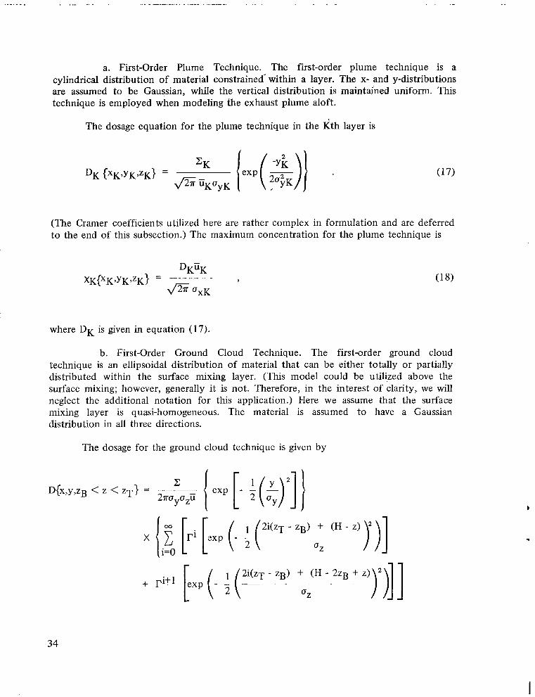
a. First-Order Plume Technique. The first-order plume technique is a cylindrical distribution of material constrained- within a layer. The x- and y-distributions are assumed to be Gaussian, while the vertical distribution is maintahed uniform. This technique is employed when modeling the exhaust plume aloft.

The dosage equation for the plume technique in the Kth layer is

(The Cramer coefficients utilized here are rather complex in formulation and are deferred to the end of this subsection.) The maximum concentration for the plume technique is

where DK is given in equation (17).

b. First-Order Ground Cloud Technique. The first-order ground cloud technique is an ellipsoidal distribution of material that can be either totally or partially distributed within the surface mixing layer. (This model could be utilized above the surface mixing; however, generally it is not. Therefore, in the interest of clarity, we will neglect the additional notation for this application.) Here we assume that the surface mixing layer is quasi-homogeneous. The material is assumed to have a Gaussian distribution in all three directions.

The dosage for the ground cloud technique is given by

34

I

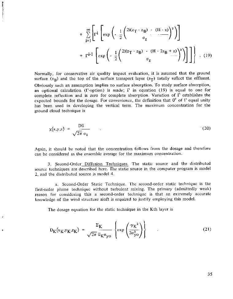
00 2 i ( Z ~- ZB)~. (H - Z))')]-+ cr i i= 1 (3Z

r

Normally, for conservative air quality impact evaluation, it is assumed that the ground surface (ZB) and the top of the surface transport layer (ZT) totally reflect the effluent. Obviously such an assumption implies no surface absorption. To study surface absorption, an optional calculation (I?-option) is made; I? in equation (19) is equal to one for complete reflection and is zero for complete absorption. Variation of I? establishes the expected bounds for the dosage. For convenience, the definition that 0" of .I? equal unity has been used in developing the vertical term. The maximum concentration for the ground cloud technique is

Again, it should be noted that the concentration follows from the dosage and therefore can be considered as the ensemble average for the maximum concentration.

3. Second-Order Diffusion Techniques. The static source and the distributed source techniques are described here. The static source in the computer program is model 2, and the distributed source is model 4.

a. Second-Order Static Technique. The second-order static technique is the first-order plume technique without turbulent mixing. The primary (admittedly weak) reason for considering this a second-order technique is that an extremely accurate knowledge of the wind structure aloft is required to justify employing this model.

The dosage equation for the static technique in the Kth layer is

35

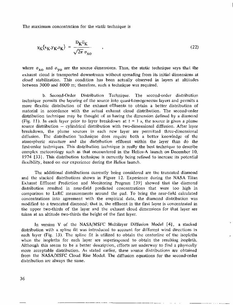
The maximum concentration for the static technique is

where axo and ayo are the source dimensions. Thus, the static technique says that the exhaust cloud is transported downstream without spreading from its initial dimensions at cloud stabilization. This condition has been actually observed in layers at altitudes between 3000 and 8000 m; therefore, such a technique was required.

b. Second-Order Distribution Technique. The second-order distribution technique permits the layering of the source into quasi-homogeneous layers and permits a more flexible distribution of the exhaust effluents to obtain a better distribution of material in accordance with the actual exhaust cloud distribution. The second-order distribution technique may be thought of as having the dimension defined by a diamond (Fig. 11). In each layer prior to layer breakdown at t = 1 s, the source is given a plume source distribution - cylindrical distribution with two-dimensional diffusion. After layer breakdown, the plume sources in each new layer are permitted three-dimensional diffusion. The distribution 'technique does require both a better knowledge of the atmospheric structure and the distribution effluent within the layer than do the first-order techniques. This distribution technique is really the best technique to describe complex meteorology such as that encountered in the Helios-A launch on December 10, 1974 [33] . This distribution technique is currently being refined to increase its potential flexibility, based on our experience during the Helios launch.

The additional distributions currently being considered are the truncated diamond and the stacked distributions shown in Figure 12. Experience during the NASA Titan Exhaust Effluent Prediction and Monitoring Program [ 3 9 ] showed that the diamond distribution resulted in near-field predicted concentrations that were too high in comparison to LaRC measurements around the pad. To bring the near-field calculated concentrations into agreement with the empirical data, the diamond distribution was modified to a truncated diamond; that is, the effluent in the first layer is concentrated in the upper two-thirds of the layer and the exhaust cloud dimensions for that layer are taken at an altitude two-thirds the height of the first layer.

In version V of the NASA/MSFC Multilayer Diffusion Model [4J,a stacked distribution with a spline fit was introduced to account for different wind directions in each layer (Fig. 13). The spline fit is utilized to obtain the centerline of the isopleths when the isopleths for each layer are superimposed to obtain the resulting isopleth. Although this seems to be a better description, efforts are underway to find a physically more acceptable distribution. As stated earlier, these source distributions are obtained from the NASA/MSFC Cloud Rise Model. The diffusion equations for the second-order distribution are always the same.

36

... . . . -.

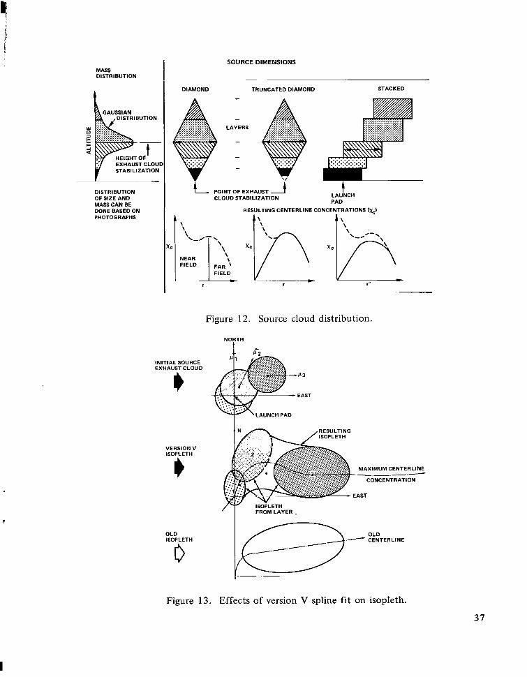
E.

SOURCE DIMENSIONS MASS DISTRIBUTION

I DIAMOND TRUNCATED DIAMOND STACKED

DISTRIBUTION

Y n 3 c

1 HAUST CLOUl STABILIZATION

DISTRIBUTION POINT OF EXHAUST 3 OF SIZE AND CLOUD STABILIZATION LAUNCH

MASS CAN BE PAD

DONE BASED ON RESULTING CENTERLINE CONCENTRATIONS ( X ) PHOTOGRAPHS

\

\

NEAR FIELD F~~ 8

FIELDI -xcb

r

INITIAL SOURCE EXHAUST CLOUD

VERSION V ISOPLETH

OLD ISOPLETH

Figure 12. Source cloud distribution.

.OrTH ;-

P 3

EAST

LAUNCH PAD

MAXIMUM CENTERLINE -. -.-.-.-----

CONCENTRATION

EAST

OLD .- CENTERLINE

I

Figure 13. Effects of version V spline fit on isopleth.

37

I

.. .

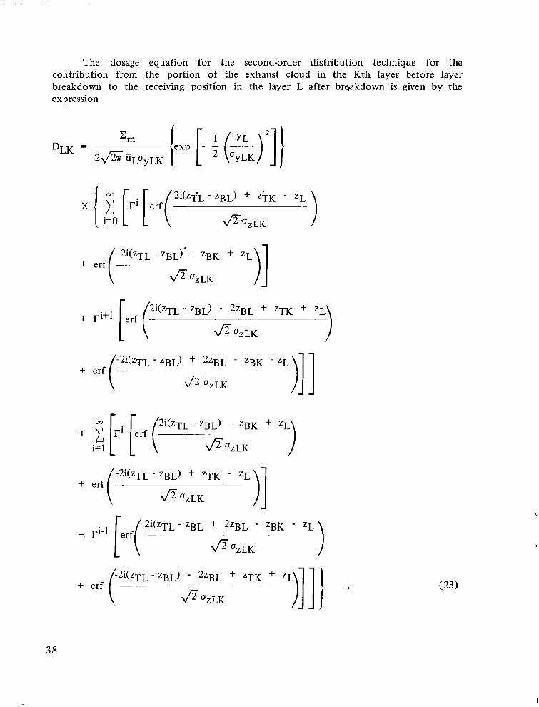
The dosage equation for the second-order distribution technique for the contribution from the portion of the exhaust cloud in the Kth layer before layer breakdown to the receiving position in the layer L after braakdown is given by the expression

38

where I? is the reflection coefficient for the surface absorption as defined with the ground cloud technique. The total dosage for the Lth layer is

N

where N is the number of older layers in the new Lth layer.

The form of the dosage algorithm in the distribution technique is similar to the form of the dosage algorithm in the ground cloud technique except that the error function is used instead of the exponential function in the vertical diffusion term. The reason for the error function in the distribution technique is to account for the comers of the expanding cylinders.

The maximum concentration algorithm for the distribution technique is

where the basic Cramer coefficients are defined at the end of this subsection.

It should be recognized that the source strength, ZK, for each layer was obtained by assuming that the effluents are distributed in a diamond distribution in version IV of this model. The effluents can be assumed to be distributed in any desired or convenient manner. In version V, the effluent mass distribution is Gaussian with constant dimensions. This is one feature of the model and is an advantage currently being studied to improve this description. Another feature in version V of the model is that the mean wind direction in each layer can be utilized in obtaining the isopleths by a spline fit of the superimposed results from each layer.

4. Diffusion Options. Three diffusion options exist - the deposition (A) option, the scavenging ( 2 )option, and the absorption (I?) option - that can be used with any of the techniques. These options represent the state of development in our ability to

? account for some of the exhaust cloud chemistry.

a. Z-Option. The Sopt ion is the option to account for precipitation scavenging (model 5 ) . The ground level deposition (D ~ K )resulting from precipitation scavenging is given basically by

39

where t l is the time the rain begins. The scavenging coefficient A for gaseous HCI obtained in laboratory tests is [431

A(HC1gas) = 1.11 X 10-4R0.625 ,

where R(mm/h) is the rate of rainfall. Results obtained in preliminary chamber tests are of approximately the same magnitude [44] ; that is,

A{HCl gas) = 8.3 X 10-5Ro-567

Since the scavenging coefficients obtained in the chamber tests were measured with all exhaust constituents present, we feel that they may be slightly more realistic because of the presence of A1203. As can be seen in Figure 14, the Al2O3 in the solid rocket exhaust effluent is of two forms: (1) a-alumina - the spheres of about 5 ,um and the larger shells, and (2) the y-alumina - small fleecy material in the background. It has been shown [45,46] that the y-alumina will react with the HCI, whereas the a-alumina does not react with the HC1. Hence, we would expect the scavenging coefficients obtained in the presence of the y-alumina to be relatively low compared to the coefficient obtained in the presence of a-alumina.

This result is more clearly illustrated in Tables 1 and 2 where these scavenging coefficients have been used to predict the acid rainout with typical baseline atmospheric data [33] .

Here the values of surface water pH were calculated from the expression

40

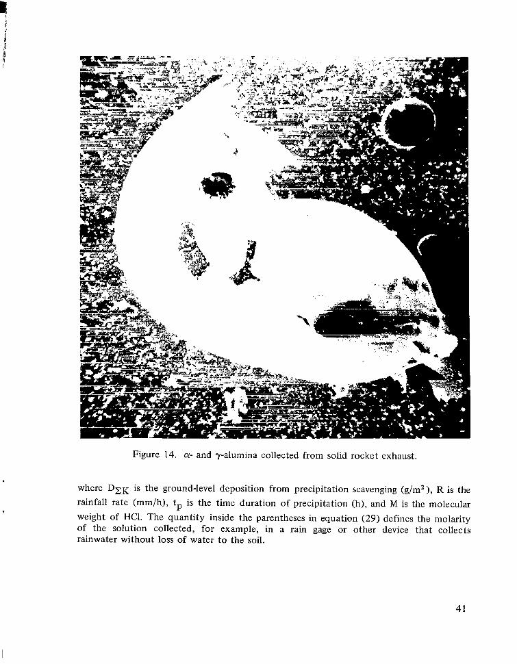
Figure 14. a-and y-alumina collected from solid rocket exhaust.

where D ~ Kis the ground-level deposition from precipitation scavenging (g/m2), R is the rainfall rate (mm/h), tp is the time duration of precipitation (h), and M is the molecular

?

weight of HC1. The quantity inside the parentheses in equation (29) defines the molarity of the solution collected, for example, in a rain gage or other device that collects rainwater without loss of water to the soil.

41

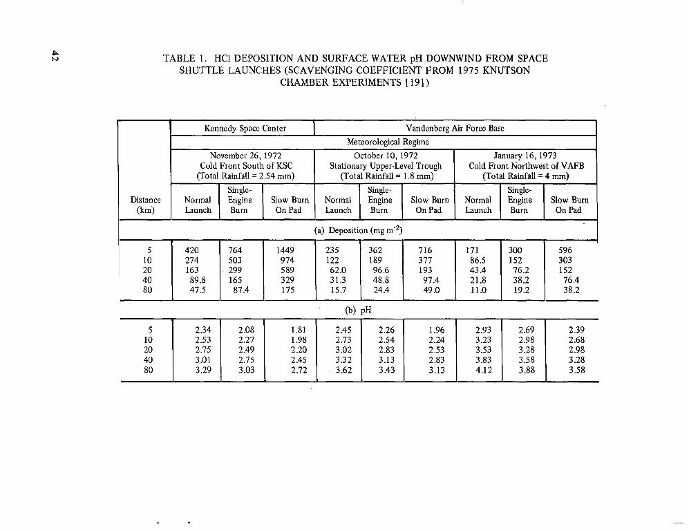
P N TABLE 1. HC1 DEPOSITION AND SURFACE WATER pH DOWNWIND FROM SPACE

SHUTTLE LAUNCHES (SCAVENGING COEFFICIENT FROM 1975 KNUTSON CHAMBER EXPERIMENTS [ 191)

>

Kennedy Space Center I Vandenberg Air Force Base Meteorological Regime

November 26,1972 Cold Front South of KSC

October 10, 1972 Stationary Upper-Level Trough

January 16,1973 Cold Front Northwest of VAFB

(Total Rainfall = 2.54 mm) (Total Rainfall = 1.8 mm) (Total Rainfall = 4 mm) Single- Single- Single-

Distance Normal Engine Slow Burn Normal Engine Slow Burn Normal Engine Slow Burn (km) Launch Burn On Pad Launch Burn On Pad Launch Burn On Pad

I

5 420

5 2.34 10 2.53 20 2.75 40 3.01 80 3.29

(a) Deposition (mg m-2)

1449 235 362 300 596

2.08 1.81 2.45 2.26 1.96 2.93 2.69 2.39 2.27 1.98 2.73 2.54 2.24 3.23 2.98 2.68 2.49 2.20 3.02 2.83 2.53 3.53 3.28 2.98 2.75 2.45 3.32 3.13 2.83 3.83 3.58 3.28 3.03 2.72 3.62 3.43 3.13 4.12 3.88 3.58

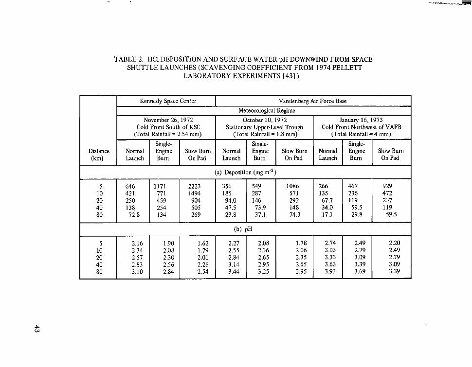
TABLE 2. HC1 DEPOSITION AND SURFACE WATER pH DOWNWIND FROM SPACE SHUTTLE LAUNCHES (SCAVENGING COEFFICIENT FROM 1974 PELLETT

LABORATORY EXPERIMENTS [43] )

Kennedy Space Center

November 26, 1972 Cold Front South of KSC

(Total Rainfall = 2.54 mm) Single-

Vandenberg Air Force Base Meteorological Regime

October 10, 1972 January 16,1973 Stationary Upper-LevelTrough Cold Front Northwest of VAFB

(Total Rainfall = 1.8 mm) (Total Rainfall = 4 mm) Single- Single-

Distance Normal Engine Slow Burn Normal Engine Slow Burn Normal Engine Slow Burn (km) Launch Bum On Pad Launch Bum On Pad Launch Burn On Pad

5 646 1171 2223 356 549 1086 266 10 42 1 77 1 1494 185 287 57 1 135 20 250 459 904 94.0 146 292 67.7 40 138, 254 505 47.5 73.9 148 34.0

467 929 236 472 119 237 59.5 119 29.8 59.5

2.49 2.20 2.79 2.49 3.09 2.79 3.39 3.09

80 72.8 134 269 23.8 37.1 74.3

5 2.16 1.90 1.62 2.27 2.08 1.78 10 2.34 2.08 1.79 2.55 2.36 2.06 20 2.57 2.30 2.01 2.84 2.65 2.35 40 2.83 2.56 2.26 3.14 2.95 2.65 80 3.10 2.84 2.54 3.44 3.25 2.95

17.1

2.74 3.03 3.33 3.63 3.93 3.69 3.39

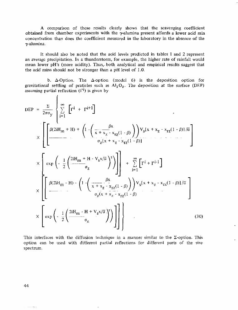
A comparison of these results clearly shows that the scavenging coefficient obtained from chamber experiments with the yalumina present affords a lower acid rain concentration than does the coefficient measured in the laboratory in the absence of the yalumina.

It should also be noted that the acid levels predicted in tables 1 and 2 represent an average precipitation. In a thunderstorm, for example, the higher rate of rainfall would mean lower pH’s (more acidity). Thus,, both analytical and empirical results suggest that the acid rains should not be stronger than a pH level of 1.0.

b. A-Option. The A-option (model 6) is the deposition option for gravitational settling of pra.ticles such as Al2O3. The deposition at the surface (DEP) assuming partial reflection (ri)is given by

DEP = [Fi + r i + l1 + H ) + (I-(­x + xz

X Oz[X

.

+ xz - X r z U - PI1 L

2iHm + H - Vsx/ii !)]I + 00

[ri + pi-11( *Z i= 1 -1

uz(x + xz - Xrz(l -

This interfaces with the diffusion technique in a manner similar to the 2-option. This option can be used with different partial reflections for different parts of the size spectrum.

44

< '

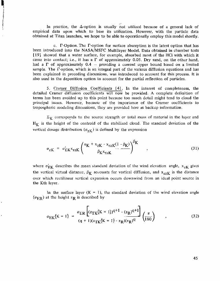
In practice, the A-option is usually not utilized because of a general lack of empirical data upon which to base its utilization. However, with the particle data obtained at Titan launches, we hope to be able to operationally employ this model shortly.

c. r-0ption.The I?-option for surface absorption is the latest option that has been introduced into the NASA/MSFC Multilayer Model. Data obtained in chamber tests [ 191 showed that a water surface, for example, absorbed most of the HC1 with which it came into contact; i.e., it has a r of approximately 0.05. Dry sand, on the other hand, had a I? of approximately 0.4 - providing a cu.rrent upper bound based on a limited sample. The r-option, which is an integral part of the various diffusion equations and has been explained in preceding discussions, was introduced to account for this process. It is also used in the deposition option to account for the partial reflection of particles.

5. Cramer Diffusion Coefficients [4 ] . In the interest of completeness, the detailed Cramer diffusion coefficients will now be provided. A complete definition of terms has been avoided up to this point because too much detail might tend to cloud the principal issues. However, because of the importance of the Cramer coefficients to tropospheric modeling discussions, they are provided here as backup information.

ZK corresponds to the source strength or total mass of material in the layer and HK is the height of the centroid of the stabilized cloud. The standard deviation of the vertical dosage distribution ( U ~ K )is defined by the expression

where D ~ Kdescribes the mean standard deviation of the wind elevation angle, X ~ Kgives the vertical virtual distance, OK accounts for vertical diffusion, and x r z ~is the distance over which rectilinear vertical expansion occurs downwind from an ideal point source in the Kth layer.

In the surface layer (K = l), the standard deviation of the wind elevation angle (DER) at the height ZR is described by

45

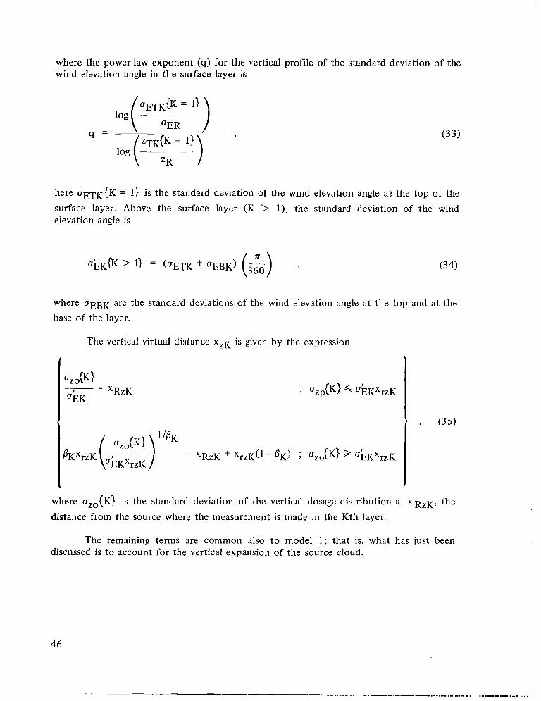
where the power-law exponent (9) for the vertical profile of the standard deviation of the wind elevation angle in the surface layer is

9 = (33)

here CJETK(K = 1) is the standard deviation of the wind elevation angle a t the top of the surface layer. Above the surface layer (K > l), the standard deviation of the wind elevation angle is

where OEBK are the standard deviations of the wind elevation angle at the top and at the base of the layer.

The vertical virtual distance X ~ Kis given by the expression

- PK) ; Ozo{K) 2 OLKXrzK

where uzo{K) is the standard deviation of the vertical dosage distribution at X R ~ K ,the distance from the source where the measurement is made in the Kth layer.

The remaining terms are common also to model 1; that is, what has just been discussed is to account for the vertical expansion of the source cloud.

46

The quantity ~ T K in equation (26) is the mean cloud transport speed in the Kth layer. In the surface layer (K = I ) , the wind speed-height profile is defined according to the power-law expression

where ~ T R is the mean wind speed measured at the reference height ZR, and the power-law exponent (p) for the wind speed profile in the surface layer is described by

here UTK{K = 1) corresponds to the mean wind speed at the top of the surface layer (ZTK{K = 1) ). Thus, in the surface layer, the mean cloud transport speed (u{K = 1)) is

which reduces to

In layers above the surface layer (K > l) , the wind speed-height profile (U(ZK, K > 1)) is assumed linear and is defined as

47

.- . .

where ~ T Kand f i g ~describe the mean wind speed at the top of the layer and at the base of the layer, respectively. In the Kth layer (K > l) , the mean cloud transport speed ( i i K { ~> I}) is

The standard deviation of the crosswind dosage distribution (ffgK) is defined by

+ [;;?I2} 9

where U ~ K ( T K }corresponds to the mean layer standard deviation of the wind azimuth for the cloud stabilization time (TK). In the surface layer (K = I ) ,

where the standard deviation of the wind azimuth angle ( u ~ R ( T K } )at height Z R and for the cloud stabilization time T K is

here U A R { T ~ K )is the standard deviation of the wind azimuth angle at height ZR and for the reference time period ( T ~ K ) ,and the power-law exponent (m) for the vertical profile of the standard deviation of the wind azimuth angle in the surface layer is

48

m =

Then,

where UATK{T ~ K ,K = 11 is the standard deviation of the wind azimuth angle at the top of the surface layer for the reference time period. For layers above the surface (K > l ) ,

where

here UATK{TK) is the standard deviation of the wind azimuth angle at the top of the layer.

here UABK{T~K) is the standard deviation of the wind azimuth angle in degrees at the base of the layer for the reference time period ( T ~ K ) .

49

The crosswind virtual distance is

when

or

when

here uYO

(K) is the standard deviation of the lateral source dimension in the layer at downwind distance X R ~ K ,XryK is the distance over which rectilinear crosswind expansion occurs downwind from an ideal point source, and CUKdescribes the lateral diffusion in the layer. The vertical wind direction shear (AOk) in the layer is

where 8TK and 8BK are the mean wind direction at the top and at the base of the layer, respectively .

The concentration algorithm is of the same form in all the techniques; however, the dosage term (DK) does depend on which technique has been utilized and thus adjusts the concentration description to the specific technique of interest.

50

The maximum concentration in the Kth layer is given by the expression

where the standard deviation of the alongwind concentration distribution ( U ~ K )in the layer is

and the alongwind cloud length (L{xK}) for a point source in the layer at the distance XK from the source is

where ATiK is the vertical wind speed shear in the layer and is defined as

or

and axo(K} is the standard deviation of the alongwind source dimension in the layer at the point of cloud stabilization. The above equation for L{xK} is based on the theoretical and empirical results reported by Tyldesley and Wallington [441 who analyzed ground-level concentration measurements made at distances of 5 to 120 km downwind from instantaneous line-source releases.

51

...-I._ ..I.

The maximum centerline concentration for the model in the Kth layer is given by the expression

The average alongwind concentration is defined as

where the ground cloud passage time in seconds is

The time mean alongwind concentration in the Kth layer is defined by the expression

where TA is the time in seconds over which concentration is to be averaged. The time mean alongwind concentration is equivalent to the average alongwind concentration when tpK equals TA.

These are only the coefficients for the first-order diffusion techniques. However, the same formulation applies to the distribution technique except that the notation is more complex. For those readers who have a further interest, your attention is directed to Reference 4, where perhaps this whole discussion should have been more appropriately directed originally.

52

D. Real-Time Diffusion Predictions

To this point, the discussion has been directed to technical performance. However, at some point, the needs of the primary user must be addressed and the technical product must be packaged in a manner that is aqpropriate to the user’s operational needs. As has been stated, the primary purpose is to afford air quality and environmental assessments for mission planning activities and for launch operations support. The diffusion predictions for the transport of the rocket exhaust effluents must utilize the same basic technique in both applications to have a meaningful cross-correlation. Since turnaround time, because of the nonstationary nature of the atmosphere, is critical in launch operational support, a system that affords a “near real-time” air quality assessment is needed for the pending launches. One vital role of actual launch prediction has been to identify the problems of such ,operational predictions and permit addressing the solutions prior to full-scale operations.

A historical review of MSFC onsite launch predictions illustrates how the techniques in predictions have evolved as a result of this launch experience. Initially, strictly mesoscale forecasting and climatological diffusion results were used to make these predictions. Experience showed a need for improvement. The climatological diffusion predictions were replaced with real-time remote computer support. The meteorological forecast was called, via telephone, from- KSC to MSFC. Some hours later (2 to 4 h), the computer diffusion predictions were relayed back to KSC and verbally given to the user. At the Titan launch in December 1973, online calculations were introduced, where the elapsed time from receipt of the rawinsonde sounding until the prediction was completed was approximately 1 to 1.5 h. In addition to the better turnaround time, the monitoring team could now be provided with graphical hard copy. This achievement was a result of the utilization of a programmable desk calculator to make predictions and provide graphical information. Since then better atmospheric measurement techniques have been introduced to obtain a description of the atmospheric kinematics (tetroonsondes, Jimsphere, and higher sampling frequency). Recognizing the continuing need to improve our techniques, another portable real-time computational system was introduced at the May 1975 Titan launch - the REEDA system (Fig. 15) - which reduces turnaround time, less than 5 min after a sounding is obtained, and uses more sophisticated modeling techniques including both the ground cloud technique and the distribution technique. The calculated diffusion predictions were limited to only a specialized ground cloud technique [ 5 ] that afforded only air quality predictions at the surface and restricted the minimum height of the surface mixing layer to the height of the exhaust cloud stabilization. Because of these restrictions, the onsite diffusion calculations were always supported with in-depth calculations at MSFC on the UNIVAC 1108 computer.

With the utilization of the REEDA system, these restrictions were overcome. The REEDA system affords the potential for the total utilization of the REED description -similar to the large computer operation, except the REEDA system also has the advantage of interactive operation and portability. The REEDA system was used instead

53

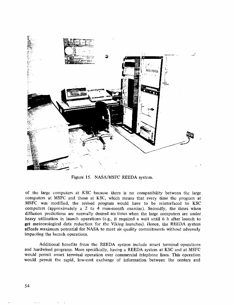
Figure 15. NASA/MSFC REEDA system.

of the large computers at KSC because there is no compatibility between the large computers at MSFC and those at KSC, which means that every time the program at MSFC was modified, the revised program would have to be reinterfaced to KSC computers (approximately a 2 to 4 man-month exercise). Secondly, the times when diffusion predictions are normally desired are times when the large computers are under heavy utilization in launch operations (e.g., it required a wait until 6 h after launch to get meteorological data reduction for the Viking launches). Hence, the REEDA system affords maximum potential for NASA to meet air quality commitments without adversely impacting the launch operations.

Additional benefits from the REEDA system include smart terminal operations and hardwired programs. More specifically, having a REEDA system at KSC and at MSFC would permit smart terminal operation over commercial telephone lines. This operation would permit the rapid, low-cost exchange of information between the centers and

54

-----

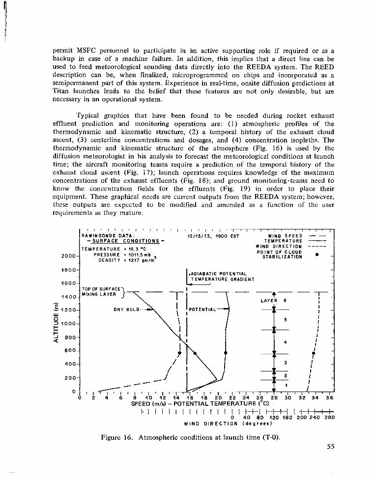
permit MSFC personnel to participate in hn active supporting role if required or as a backup in case of a machine failure. In addition, this implies that a direct line can be used to feed meteorological sounding data directly into the REEDA system. The REED description can be, when. finalized, microprogrammed on chips and incorporated as a semipermanent part of this system. Experience in real-time, onsite diffusion predictions at Titan launches leads to the belief that these features are not only desirable, but are necessary in an operational system.

Typical graphics that have been found to be needed during rocket exhaust effluent prediction and monitoring operations are: (1) atmospheric profiles of the thermodynamic and kinematic structure, (2) a temporal history of the exhaust cloud ascent, (3) centerline concentrations and dosages, and (4) concentration isopleths. The thermodynamic and kinematic structure of the atmosphere (Fig. 16) is used by the diffusion meteorologist in his analysis to forecast the meteorological conditions at launch time; the aircraft monitoring teams require a prediction of the temporal history of the exhaust cloud ascent (Fig. 17); launch operations requires knowledge of the maximum concentrations of the exhaust effluents (Fig. 18); and ground monitoring .teams need to know the concentration fields for the effluents (Fig. 19) in order to place their equipment. These graphical needs are current outputs from the REEDA system; however, these outputs are expected to be modified and amended as a function of the user requirements

I as they mature.

RAWINSONDE DATA: 12/13/73, 1900 EST WIND S P E E D --- S U R F A C E C O N D I T I O N S - TEMPERATURE -

WIND D I R E C T I O NTEMPERATURE 2 16.3 "C P O I N T OF CLOUD

2000 PRESSURE = 1011.5mb STAB I L lZATlON

18001 - + - - ,

LAYER 6 1-

I 4 I

I -

5 I I -

1I I

DENSITY = 1217 gm/m

tADIABATIC POTENTIAL

1600

I I -I4 I

6 0 0 v e I -

I 3 r'

I 2 0 0 2 I -

I I I

0 2 4 6 ' l ' l ' l ' l ' l ' l6 I O 1'2 1 4 1'6 1'8 2'0 2 2 24 26 2 8 30 3 2 34 3 6

SPEED (m/s) -POTENTIAL TEMPERATURE ("c) I

? : I I I I ! I t I I ! 1 ! ! : I 1 I I I I ! I I I I I 0 4 0 80 120 i60 200 240 280

-

W I N D D I R E C T I O N ( d e g r e e s )

Figure 16. Atmospheric conditions at launch time (T-0). 55

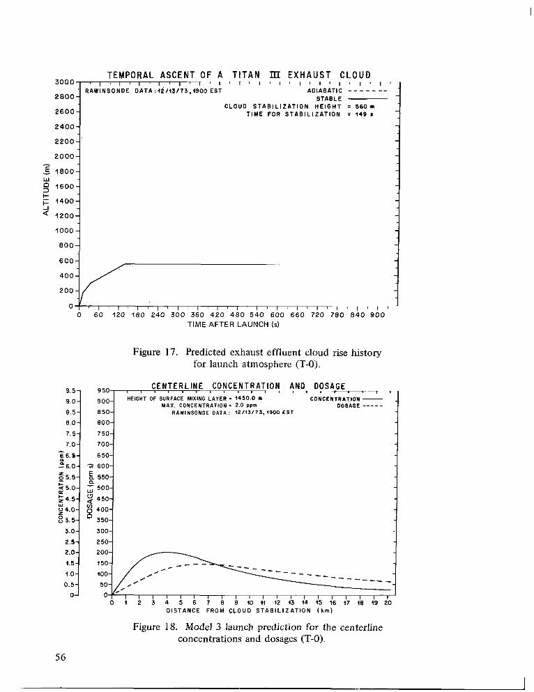
- - - TEMPORAL A S C E N T OF A TITAN IU E X H A U S T C L O U D

3000 ~ I ~ I I I ~ IT 'I l I l lI ' 1 ' 1 ' 1 1 l q l l 1 ' 1 I

. RAWINSONDE D A T A : I 2 / 1 3 / 7 3 . 1 9 0 0 EST ADIABATIC - - - - ­-2800- STABLE CLOUD S T A B I L I Z A T I O N H E I G H T = 560 m -

2600- T I M E FOR S T A B I L I Z A T I O N = 149 I

-2400­

-2200­

-2000-

E 1800- ­w5 1600- ­5 1400- -Q 1200- ­

1000- ­-800 ­

600- ­-400­

200- ­

1 ' 1 1

Figure 17. Predicted exhaust effluent cloud rise history for launch atmosphere (T-0).

C E NT E R L IN E CONCE N T R AT ION AND DOSAGE 9.5- 9 50 , , I I , , I I I f I I , I r , , - T T

9 .0 - HEIGHT OF SURFACE MIXING LAYER = 1450.0 m CONCENTRATION - -MAX. CONCENTRATION = 2.0 PPln DOSAGE ----­

8.5- 8 5 0 - RAWINSONDE DATA: 12/13173,1900 EST

8.0- 800­

7 .5 - 750­

-7.0- 700­

g6.5- 6 50­0-6 .0 - ;i600­

$5.5- 550­

25.0- 500- K

5 4 . 5 - 2 450-W p4.0- $ 400­

8 3 . 5 - 350­

3.0- 300­

2.5- 2 50­

2.0­

1.5­

1.0­ - - - _ _----_0.5­

0- , I ' I 1 I I I I I I , I I I I I ,~0 I 2 3 4 5 6 7 8 9 IO l i 12 13 14 15 16 17 I8 I9 20

DISTANCE FROM CLOUD S T A B I L I Z A T I O N ( k m )

Figure 12). Model 3 launch prediction for the centerline concentrations and dosages (T-0).

56

.-I

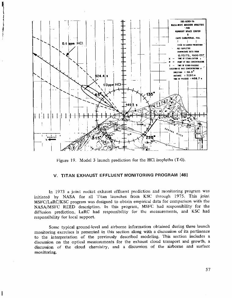
1ii1 ­

24.41s I

Figure 19. Model 3 launch prediction for the HC1. isopleths (T-0).

V. TITAN EXHAUST EFFLUENT MONITORING PROGRAM [46]

In 1973 a joint rocket exhaust effluent prediction and monitoring program was initiated by NASA for all Titan launches from KSC through 1975. This joint MSFC/LaRC/KSC program was designed to obtain empirical data for comparison with the NASA/MSFC REED description. In this program, MSFC had responsibility for the diffusion prediction, LaRC had responsibility for the measurements, and KSC had responsibility for local support.

Some typical ground-level and airborne information obtained during these launch monitoring exercises is presented in this section along with a discussion of its pertinence to the interpretation of the previously described modeling. This section includes a discussion on the optical measurements for the exhaust cloud transport and growth, a discussion of the cloud chemistry, and a discussion of the airborne and surface monitoring.

57

I

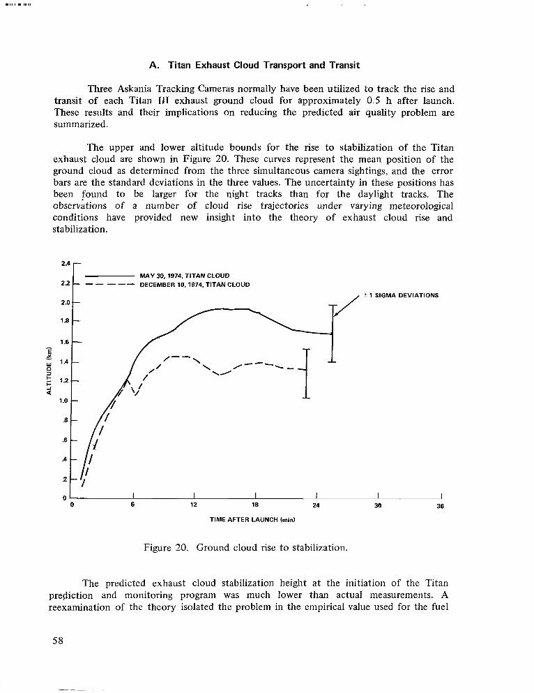
E

A. Titan Exhaust Cloud Transport and Transit

Three Askania Tracking Cameras normally have been utilized to track the rise and transit of each Titan I11 exhaust ground cloud for approximately 0.5 h after launch. These results and their implications on reducing the predicted air quality problem are summarized.

The upper and lower altitude bounds for the rise to stabilization of the Titan exhaust cloud are shown in Figure 20. These curves represent the mean position of the ground cloud as determined from the three simultaneous camera sightings, and the error bars are the standard deviations in the three values. The uncertainty in these positions has been found to be larger for the night tracks than for the daylight tracks. The observations of a number of cloud rise trajectories under varying meteorological conditions have provided new insight into the theory of exhaust cloud rise and stabilization.

MAY 30,1974, TITAN CLOUD DECEMBER 10,1974, TITAN CLOUD

2.0 c f 1 SIGMA DEVIATIONS

--Y

0 I I I I I 0 6 12 18 24 30 36

TIME AFTER LAUNCH (min)

Figure 20. Ground cloud rise to stabilization.

The predicted exhaust cloud stabilization height at the initiation of the Titan prediction and monitoring program was much lower than actual measurements. A reexamination of the theory isolated the problem in the empirical value used for the fuel

58

I

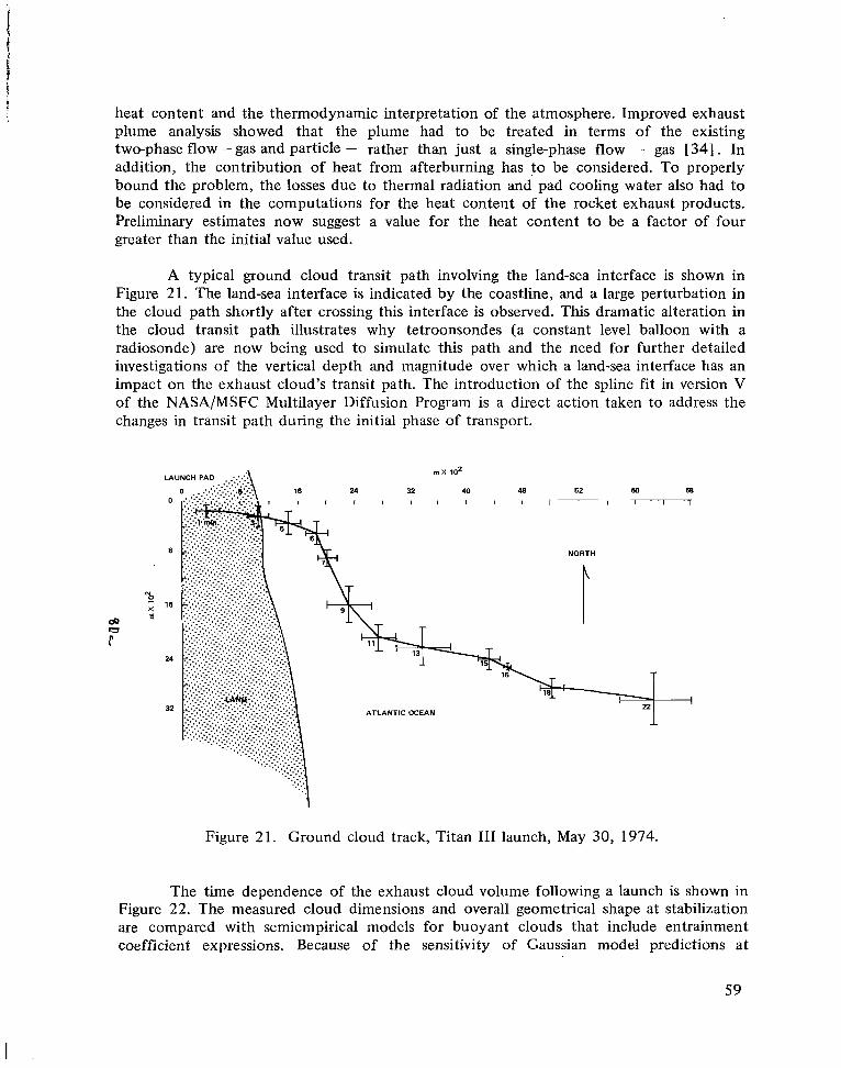
heat content and the thermodynamic interpretation of the atmosphere. Improved exhaust plume analysis showed that the plume had to be treated in terms of the existing two-phase flow -gas and particle - rather than just a single-phase flow - gas [34]. In addition, the contribution of heat from afterburning has to be considered. To properly bound the problem, the losses due to thermal radiation and pad cooling water also had to be considered in the computations for the heat content of the rocket exhaust products. Preliminary estimates now suggest a value for the heat content to be a factor of four greater than the initial value used.

A typical ground cloud transit path involving the land-sea interface is shown in Figure 2 1 . The land-sea interface is indicated by the coastline, and a large perturbation in the cloud path shortly after crossing this interface is observed. This dramatic alteration in the cloud transit path illustrates why tetroonsondes (a constant level balloon with a radiosonde) are now being used to simulate this path and the need for further detailed investigations of the vertical depth and magnitude over which a land-sea interface has an impact on the exhaust cloud’s transit path. The introduction of the spline fit in version V of the NASA/MSFC Multilayer Diffusion Program is a direct action taken to address the changes in transit path during the initial phase of transport.

m X 102

24 32 40 48 52 60 a ....._.....,- . .-,...J . 1 1 1 1 1 I 1 1 I 1 1 1 I I I T

NORTH

Na X E

ATLANTIC OCEAN .L

Figure 21. Ground cloud track, Titan I11 launch, May 30, 1974.

The time dependence of the exhaust cloud volume following a launch is shown in Figure 22. The measured cloud dimensions and overall geometrical shape at stabilization are compared with semiempirical models for buoyant clouds that include entrainment coefficient expressions. Because of the sensitivity of Gaussian model predictions at

59

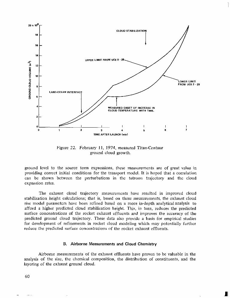
0

-20 x 108

CLOUD STABILIZATION

18 ­

-16 I 14 -

UPPER LIMIT FROM UCS 9 - 26 65.5

E 1 2 -W

5 2 -g0 3

10

LOWER LIMIT 2 0 8 -0 23 LAND-OCEAN INTERFACE

6 ­

4- MEASURED ONSET OF INCREASE IN CLOUD TEMPERATURE WITH TIME.

2 ­

0 I I 0 1 2 3 4 5 6 7

TIME AFTER LAUNCH ( m i d

Figure 22. February 1 1, 1974, measured Titan-Centaur ground cloud growth.

ground level to the source term expressions, these measurements are of great value in providing correct initial conditions for the transport model. It is hoped that a correlation can be shown between the perturbations in the tetroon trajectory and the cloud expansion rates.

The exhaust cloud trajectory measurements have resulted in improved cloud stabilization height calculations; that is, based on these measurements, the exhaust cloud rise model parameters have been refined based on a more in-depth analyticalanalysis to afford a higher predicted cloud stabilization height. This, in turn, reduces the predicted surface concentrations of the rocket exhaust effluents and improves the accuracy of the predicted ground cloud trajectory. These data also provide a basis for empirical studies for development of refinements in rocket cloud modeling which may potentially further reduce the predicted surface concentrations of the rocket exhaust effluents.

B. Airborne Measurements and Cloud Chemistry

Airborne measurements of the exhaust effluents have proven to be valuable in the analysis of the size, the chemical composition, the distribution of constituents, and the layering of the exhaust ground cloud.

60

111

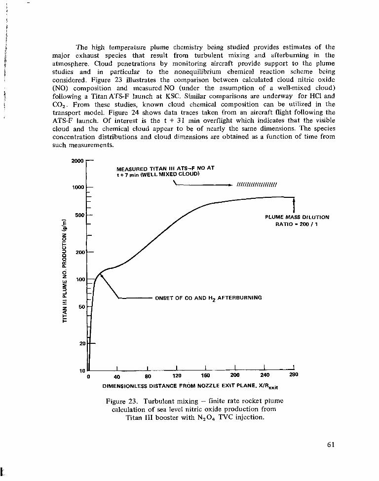
The high temperature plume chemistry being studied provides estimates of the major exhaust species that result from turbulent mixing and afterburning in the atmosphere. Cloud penetrations by monitoring aircraft provide support to the plume studies and in particular to the nonequilibrium chemical reaction scheme being considered. Figure 23 illustrates the comparison between calculated cloud nitric oxide (NO) composition and measured NO (under the assumption of a well-mixed cloud) following a Titan ATS-F launch at KSC. Similar comparisons are underway for HCl and COz. From these studies, known cloud chemical composition can be utilized in the transport model. Figure 24 shows data traces taken from an aircraft flight following the ATS-F launch. Of interest is the t + 31 min overflight which indicates that the visible cloud and the chemical cloud appear to be of nearly the same dimensions. The species concentration distributions and cloud dimensions are obtained as a function of time from such measurements.

MEASURED TITAN 111 ATS-F NO AT t + 7 min (WELL MIXED CLOUD)

1000 t

0z

0 40 80 120

DIMENSIONLESS DISTANCE FROM NOZZLE EXIT PLANE, X/R,,it

Figure 23. Turbulent mixing - finite rate rocket plume calculation of sea level nitric oxide production from

Titan I11 booster with NzO, TVC injection.

61

111.

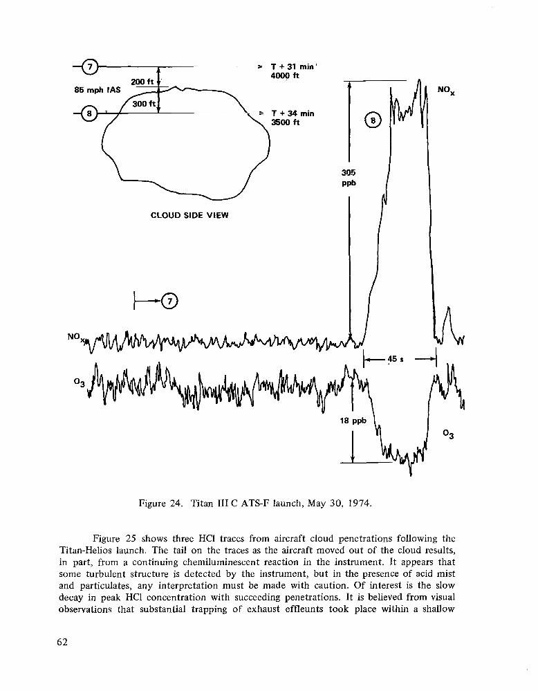
T + 3 1 min' 4000 ft

T + 34min 3500*

305 PPb

CLOUD SIDE VIEW i NO

Figure 24. Titan I11 C ATS-F launch, May 30, 1974.

Figure 25 shows three HCI traces from aircraft cloud penetrations following the Titan-Helios launch. The tail on the traces as the aircraft moved out of the cloud results, in part, from a continuing chemiluminescent reaction in the instrument. It appears that some turbulent structure is detected by the instrument, but in the presence of acid mist and particulates, any interpretation must be made with caution. Of interest is the slow decay in peak HC1 concentration with succeeding penetrations. It is believed from visual observations that substantial trapping of exhaust effleunts took place within a shallow

62

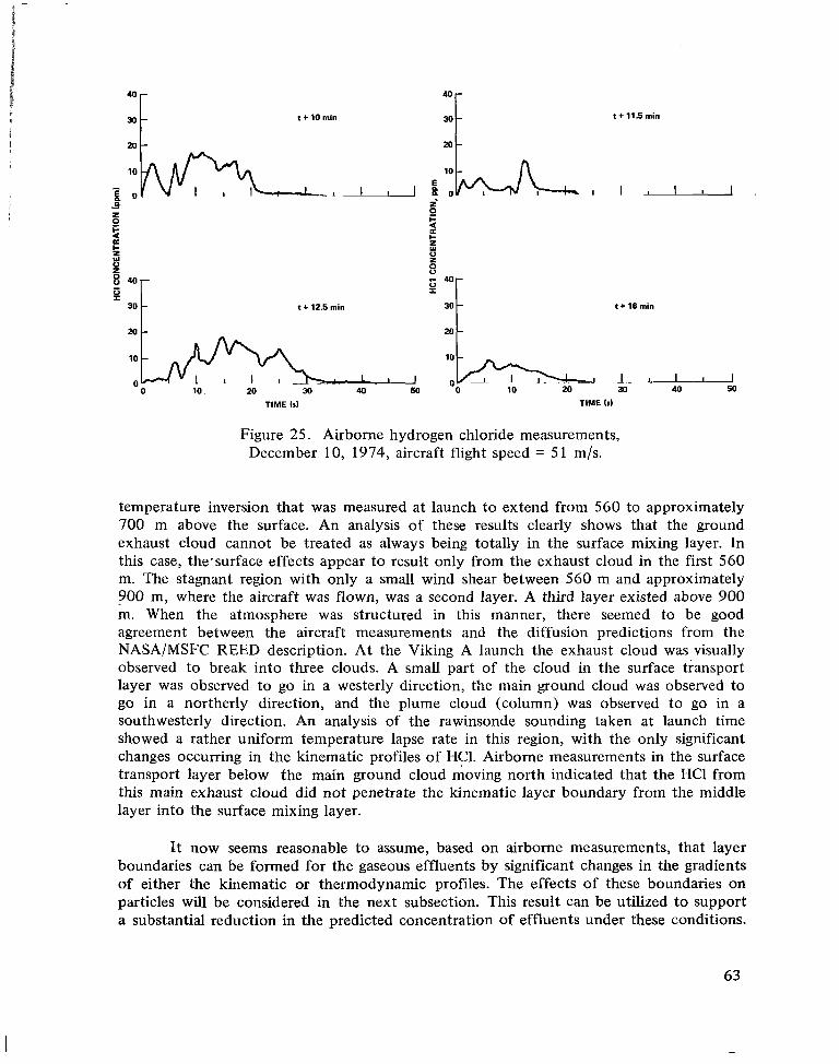
t + 10min

20‘E 40

t + 11.5min

20301 I I L

t + 16 min

Fz

z 840-1 t + 12.5 min %t

TIME (11 TIME (5)

Figure 25. Airborne hydrogen chloride measurements, December 10, 1974, aircraft flight speed = 5 1 m/s.

temperature inversion that was measured at launch to extend from 560 to approximately 700 m above the surface. An analysis of these results clearly shows that the ground exhaust cloud cannot be treated as always being totally in the surface mixing layer. In this case, the.surface effects appear to result only from the exhaust cloud in the first 560 m. The stagnant region with only a small wind shear between 560 m and approximately 900 m, where the aircraft was flown, was a second layer. A third layer existed above 900 m. When the atmosphere was structured in this manner, there seemed to be good agreement between the aircraft measurements and the diffusion predictions from the NASA/MSFC REED description. At the Viking A launch the exhaust cloud was visually observed to break into three clouds. A small part of the cloud in the surface transport layer was observed to go in a westerly direction, the main ground cloud was observed to go in a northerly direction, and the plume cloud (column) was observed to go in a southwesterly direction, An analysis of the rawinsonde sounding taken at launch time showed a rather uniform temperature lapse rate in this region, with the only significant changes occurring in the kinematic profiles of HC1. Airborne measurements in the surface transport layer below the main ground cloud moving north indicated that the HC1 from this main exhaust cloud did not penetrate the kinematic layer boundary from the middle layer into the surface mixing layer.

It now seems reasonable to assume, based on airborne measurements, that layer boundaries can be formed for the gaseous effluents by significant changes in the gradients of either the kinematic or thermodynamic profiles. The effects of these boundaries on particles will be considered in the next subsection. This result can be utilized to support a substantial reduction in the predicted concentration of effluents under these conditions.

63

8

C. Surface Monitoring

A large amount of information has been collected on surface concentrations of the exhaust constituents ' (hydrogen chloride, carbon dioxide, carbon monoxide, and aluminum oxide) during the seven launches in the Titan Exhaust' Effluent Prediction and

. Monitoring Program at KSC. Much of the data is still being compiled and analyzed; however, there are some significant facts relevant to modeling that are already apparent that will be discussed here.

Hydrogen chloride is the signature constituent for the dispersive gaseous transport of the exhaust effluent, with the aluminum oxide serving as a supporting constituent in the data analysis because of particle behavior. Since it was found that the surface concentrations of carbon dioxide were so low as to be within. normal variations, these measurements were dropped after the first few launches. Measurements of carbon monoxide were found to be more meaningful; however, it was difficult to always correlate the carbon monoxide measurements with the transport of the exhaust effluents. This correlation with the effluents cannot be established with carbon monoxide-since there are some potential sources for its emission around the launch area, such as the internal combustion engine, whereas, the solid rocket motors of the launch vehicle are the only significant source for hydrogen chloride; hence, hydrogen chloride is selected as the rocket exhaust signature constituent.

The NASA/MSFC REED predictions are a function of meteorological input data. Meteorological conditions described by the input data may not accurately represent conditions encountered by the effluent cloud. In this situation the model will inaccurately calculate the expected ground level concentration; thus, the calculated values will deviate from ground-level measurements. These deviations are attributable to uncertainties in our knowledge of the meteorological conditions rather than to uncertainties in the diffusion model. Therefore, it can be concluded that any comparison of model predictions with ambient measurements must include a study of the adequacy of the description of meteorological conditions responsible for plume dispersion and transport. The services of a NASA/MSFC REED program meteorologist to monitor the meteorological input and assist in interpretation of the REED predictions are very important.

The comparison between the hydrogen chloride measurements made by LaRC and the air quality prediction from the NASA/MSFC REED description during the Titan Rocket Exhaust Effluent Prediction and Monitoring Program was excellent. For the 40 ground sites where hydrogen chloride data were taken, the predicted concentrations at the site ranges were either higher or within the predicted limits in all cases. However, accordin$ to Dr. G. Gregory, LaRC, if the same data set is compared both in range and azimuth, there are 21 cases where the predicted concentrations from the NASAlMSFC REED description were high, 16 cases where the predictions were within limits, and 3 cases where the predictions were low. In some of the cases where the NASA/MSFC REED description predicted higher concentrations of hydrogen chloride than were measured, the site may not have been operating at the time the exhaust cloud passed

1. Personal communication with author.

64

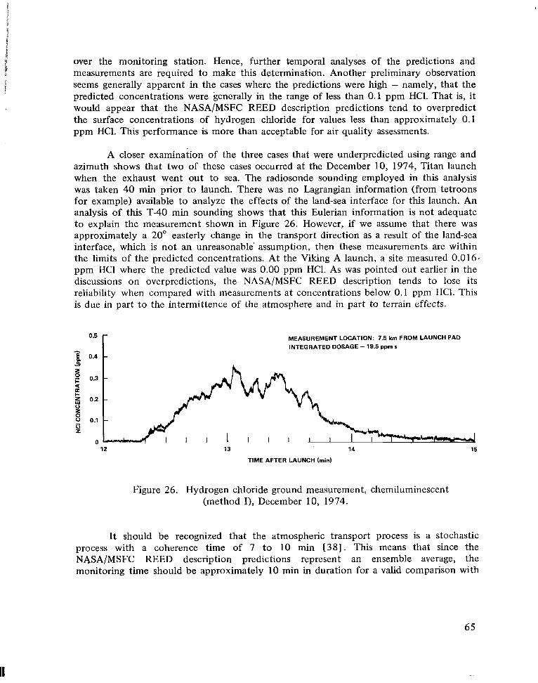
over the monitoring station. Hence, further temporal analyses of the predictions and measurements are required to make this determination. Another preliminary observation seems generally apparent in the cases where the predictions were high - namely, that the predicted concentrations were generally in the range of less than 0.1 ppm HC1. That is, it would appear that the NASA/MSFC REED description predictions tend to overpredict the surface concentrations of hydrogen chloride for values less than approximately 0.1 ppm HC1. This performance is more than acceptable for air quality assessments.

A closer examination of the three cases that were underpredicted using range and azimuth shows that two of these cases occurred at the December 10, 1974, Titan launch when the exhaust went out to sea. The radiosonde sounding employed in this analysis was taken 40 min prior to launch. There was no Lagrangian information (from tetroons for example) available to analyze the effects of the land-sea interface for this launch. An analysis of this T-40 min sounding shows that this Eulerian information is not adequate to explain the measurement shown in Figure 26. However, if we assume that there was approximately a 20" easterly change in the transport direction as a result of the land-sea interface, which is not an unreasonable' assumption, then these measurements are within the limits of the predicted concentrations. At the Viking A launch, a site measured 0.016, ppm HC1 where the predicted value was 0.00 ppm HC1. As was pointed out earlier in the discussions on overpredictions, the NASAlMSFC REED description tends to lose its reliability when compared with measurements at concentrations below 0.1 ppm HC1. This is due in part t o the intermittence of the atmosphere and in part to terrain effects.

MEASUREMENT LOCATION: 7.5 km FROM LAUNCH PAD ob r INTEGRATED DOSAGE - 19.5 ppm Ic

B5 0.3

2 I-$ O2 z 8 0.1

H 0

12 13 14 15

TIME AFTER LAUNCH ( m i d

Figure 26. Hydrogen chloride ground measurement, chemiluminescent (method I), December 10, 1974.

It should be recognized that the atmospheric transport process is a stochastic process with a coherence time of 7 to 10 min [38 ] . This means that since the NASA/MSFC REED description predictions represent an ensemble average, the monitoring time should be approximately 10 min in duration for a valid comparison with

65

a measurement. Thus, the peak concentration should compare more favorably with measurements such as these with durations less than the coherence time than with the predicted dosage. In practice, this appears to happen; that is, the predicted dosages measured during this program were always considerably greater than the measured values. In aerospace air quality applications, a high prediction of the dosage does not present a problem to its use in support of launch operations.

Specifically, it now appears that according to the analysis conducted to date, near-field (less than 20 km) is the principal area of relatively high HC1 concentration. The National Academy of Sciences’ recommended ceiling value of 8 ppm HCl is the most probable air quality constraint of concern in the near field, since the time-averaged value of 4 ppm HC1 for 10 min [47] allows the averaging over periods that normally exceed the significant time of exhaust cloud passage. Ilence, the primary concern in aerospace vehicle air quality investigations is peak concentrations rather than dosages.

The NASA Rocket Exhaust Effluent Prediction and Monitoring Program has resulted in a significant refinement in the predicted concentrations in the first few kilometers around the launch pad. Photographic and optical observations suggest that a small part of the bottom of the ground exhaust cloud might actually never leave the ground and thus be transported along the surface. However, based on a number of null hydrogen chloride measurements around the pad, it can be assumed that all of the effluents initially leave the surface. This is another result of this program that has been incorporated into version V of the NASA/MSFC Multilayer Diffusion Program.

Information on scavenging of HC1 by a thunderstorm was obtained at the Viking B launch. Accordin2to Dr. G. Pellett, LaRC, the preliminary results from his chemical analysis show a pH of 1.0 at one site and a pH of 1.4 at the other site. The strongest predicted concentration by the NASA/MSFC REED description on similar data but for only a medium rain was a pH of 1.8. Thus, it is necessary to examine the current scavenging option in the NASAlMSFC Multilayer Diffusion Model and adjust it for thundershowers.

The current A1203 deposition option in the model is in need of updating. This deposition option is basically not being used, and the A1203 is being treated as a gas. Preliminary results of the monitoring show that when the A1203 measurements are analyzed by the deposition option, we should be able to initially account for gravitational settling by particle size.

Extensive photographic documentation of the exhaust clouds was made during daylight launches, and infrared imaging was used to obtain thermal signatures from the cloud as well as continuous distant (up to 40 km) cloud images. The exhaust cloud dimensions can be obtained from imaging and compared with predicted growth. Figure 27 shows “instantaneous” cloud crosswind dimensions from two launch monitoring exercises. Virtual source dimensions are obtained, as well as details of the vertical diffusion patterns as the cloud moves with the wind. Both clouds exhibit a total crosswind divergence of approximately 5.5” from their virtual sources. Similar studies of

2. Personal communication with author.

66

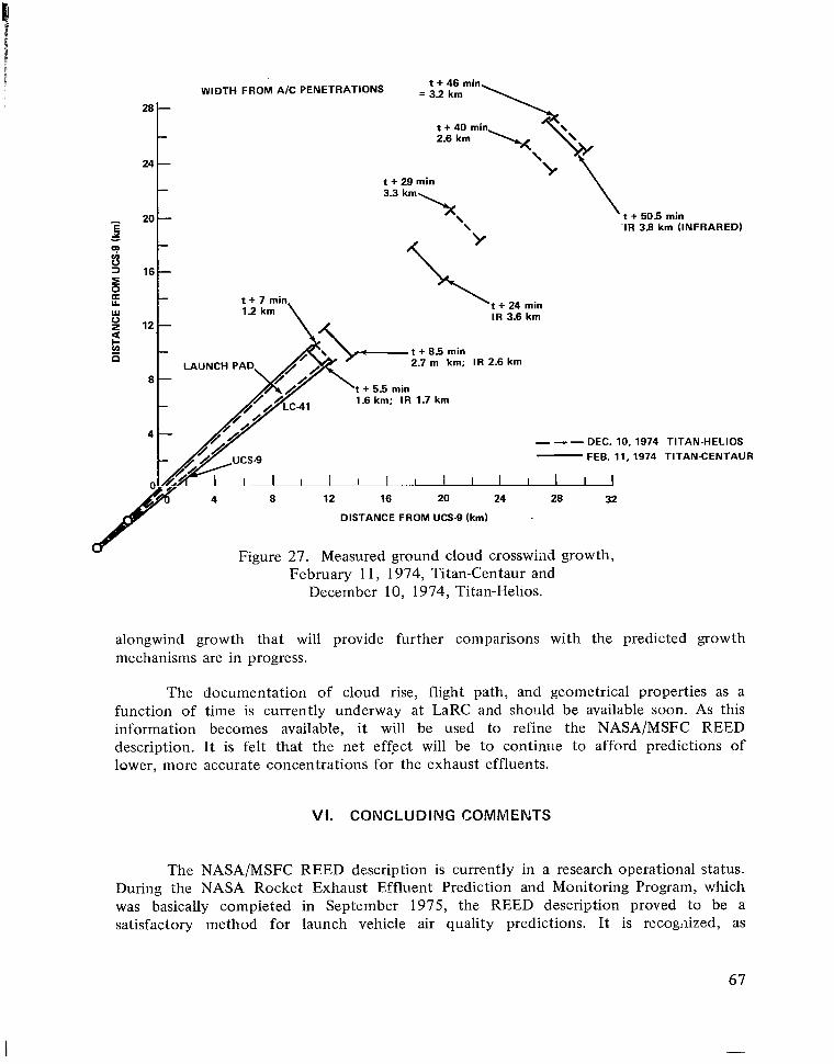
km;

t + 46 minWIDTH FROM A/C PENETRATIONS = 32 km

28­

- t + 29 min ““:-t\-24

-

\20 - 3-3“”\.x t + 505 min \ -IR 3.8 km ( INFRARED)

t + 7 min 1 2 k m \ t + 24 min

IR 3.6 km

1 \-+ 8 5 min IR 2.6 kmt2.7 m L A U N C H P A D / ,

I ’ / ’ / t + 5 5 min

L C 4 1 1.6 km; I R 1.7 km

/ / 4 - ,//’ ---DEC. 10, 1974 TITAN-HELIOS-- ,//’ u c s - 9 FEB. 11, 1974 T ITANCENTAUR

I

8 12 16 20 24 28 32

DISTANCE FROM UCS-9 (km)

Figure 27. Measured ground cloud crosswiilil growth, February 11, 1974, Titan-Centaur and

December 10, 1974, Titan-Helios.

alongwind growth that will provide further comparisons with the predicted growth mechanisms are in progress.

The documentation of cloud rise, flight path, and geometrical properties as a function of time is currently underway at LaRC and should be available soon. As this information becomes available, it will be used to refine the NASAlMSFC REED description. It is felt that the net effect will be to continue to afford predictions of lower, more accurate concentrations for the exhaust effluents.

VI. CONCLUDING COMMENTS

The NASA/MSFC REED description is currently in a research operational status. During the NASA Rocket Exhaust Effluent Prediction and Monitoring Program, which was basically compieted in September 1975, the REED description proved to be a satisfactory method for launch vehicle air quality predictions. It is recogiiized, as

67

discussed in Section VI, that there are areas where the REED description can be refined; however, the fundamental structure for the description of exhaust effluent diffusion does appear to be sound. A diagnostic mesoscale model that predicts the transit path represents the most significant refinement needed for the REED description. The surface loading effects from launch vehicle propulsion system effluents associated with HCl absorption, acid rainout, and the deposition of A1203 are areas where additional investigations are required to support ecological investigations and assessments. Further studies will improve the chemical species description for the exhaust cloud source and their relative emission rates. Finally, the current research REED description along with refinements must be converted into an operational program to regularly support launch operations on a real-time basis.

A potential alternate approach to the current NASA/MSFC REED description is to develop a numerical diffusion model. This is essentially a primitive equation mesoscale model that does not utilize simplifying assumptions on the basic equations such as are utilized with the Gaussian distribution approach used in the REED description. Although more realistic effluent distributions and cloud transit paths are advantages associated with numerical models, disadvantages include requirements for detailed meteorological inputs and an extremely large computer (250K to 750K) core. These requirements may not be easily satisfied in the operational mode. Therefore, the effective use of a numerical model in an operational mode for real-time support of launch operations is questionable. The use of a diagnostic model (a primitive equation model with simplifying assumptions) does afford the potential to combine the best feature of the Gaussian distribution model for diffusion and that of the numerical model for transport.

In summary, the REED description, in its current state of evolution, provides a research operational capability for reliable air quality prediction to support most aerospace mission planning activites and launch operations. The future activities are primarily designed to narrow the bounds on some peripheral uncertainties concerning surface loading and effluent cloud transit path. Simultaneously, there is a need to continue to evolve the REED description to an operational status.

George C. Marshall Space Flight Center National Aeronautics and Space Administration

Marshall Space Flight Center, Alabama 35812, May 1976

6 8

REFERENCES

1. National Environmental Policy Act. Public Law 91-190, 42nd U.S. Congress, 4321, 1969.

2. U.S. Clean Air Act. As amended by Public Law 91-604, 42nd U.S. Congress, 1857-18571, 1971.

3. Dumbauld, R. K.; Bjorklund, J. R.; and Bowers, J. F.: NASA/MSFC Multilayer Diffusion Models and Computer Program for Operational Prediction of Toxic Fuel Hazards. NASA CR-129006, prepared for Marshall Space Flight Center by H. E. Cramer Co., June 1973.

4. Dumbauld, R. K. and Bjorklund, J. R.: NASA/MSFC Multilayer Diffusion Models and Computer Programs - Version 5. NASA CR-2631, prepared for Marshall Space Flight Center by H. E. Cramer Co., Dec. 1975.

5. Stephens, J. Briscoe and Hamilton, P. A.: Diffusion Algorithms and Data Reduction Routine for Onsite Launch Predictions for the Transport of Titan I11 C Exhaust Effluents. NASA TN D-7862, Marshall Space Flight Center, Dec. 1974.

6. Stewart, Roger B. and Grose, William L.: Parametric Studies with an Atmospheric Diffusion Model that Assesses Toxic Fuel Hazards Due to the Ground Clouds Generated by Rocket Launches. NASA TN D-7852, Langley Research Center, Dec. 1974.

7. Gregory, Gerald L.; Hulten, William C.; and Wornom, Dewey E.: Apollo Saturn 51 1 Effluent Measurements from the Apollo 16 Launch Operations - An Experiment. NASA TM X-29 10, Langley Research Center, March 1974.

8. Hulten, William C. et al.: Effluent Sampling of Scout “D” and Delta Launch Vehicle Exhausts. NASA TM X-2987, Langley Research Center, July 1974.

9. Gregory, Gerald L.; Hudgins, Charles H.; and Emerson, Burt R., Jr.: Evaluation of a Chemiluminescent Hydrogen Chloride and a NDIR Carbon Monoxide Detector for Environmental Monitoring. 1974 JANNAF Propulsion Meeting, San Diego, CA, Oct. 22-24, 1974.

10. Stephens, J . Briscoe, ed.: Atmospheric Diffusion Predictions for the Exhaust Effluents from the Launch of a Titan I1 C, Dec. 13, 1973. NASA TM X-64925, Marshall Space Flight Center, Sept. 1974.

11. Environmental Statement for the Space Shuttle. National Aeronautics and Space Administration, July 1972.

69

REFERENCES (Continued)

12.

13.

14.

15.

16.

17.

18.

19.

20.

21.

22.

Slade, D. H., ed.: Meteorology and Atomic Energy 1968. U.S. Atomic Energy Commission, 1968.

Pasquill, F.: Atmospheric Diffusion. D. Van Nostrand Co. Ltd., London, 1962.

Barad,'M. L., ed.: Project Prairie Grass, A Field Program in Diffusion. Geophysical Research Papers No. 59, Vols. I and 11, AD-152572 and 152573, Air Force Cambridge Research Center, 1958.

Tamer, Wilson B., Jr. : Atlantic Missile Range Reference Atmosphere for Cape Kennedy, Florida, Part I. IRIG Document 104-63, Inter Range Instrumentation Group, ASTIA, 1963.

Automatic Data Acquisition System for the NASA 150 Meter Ground Winds Tower Facility, Kennedy Space Center. Final Technical Report, Vol. I, NASA Contract No. NAS26212, prepared for George C. Marshall Space Flight Center by Southwest Research Institute, San Antonio, TX, 1971.

Winds Aloft Summary and Parameters. Card Deck 600, Station 12868, Cape Kennedy, Florida, U.S. Department of Commerce, Environmental Science Services Administration, Environmental Data Service (Book 1 of 2), June 2, 1969.

Kaufman, J. W. and Keene, L. E.: NASA's 150 Meter Meteorological Tower Located at the Kennedy Space Center, Florida. NASA TM X-53699, Marshall Space Flight Center, 1968.

Knutson, E. 0. and Fenton, D. L.: Atmospheric Scavenging of Hydrochloric Acid. NASA CR-2598, prepared for George C. Marshall Space Flight Center by IIT Research Institute, Aug. 1975.

Haugen, Dcane A.; Fuquay, James J.; and Taylor, John H.: The Ocean Breeze and Dry Gulch Diffusion Programs. Vols. I and 11, prepared for Defense Documentation Center, Defense Supply Agency by General Electric Co., No. AD 428 436, 1963.

Cramer, H. E. et al.: The Study of Diffusion of Gases or Aerosols in the Lower Atmosphere. MIT Dept. of Meteorology, Contract AF 19(604)-1058, AFCRC TR 58-239, 1958.

Lulley, John L. and Panofsky, Han A.: The Structure of Atmospheric Turbulence. Interscience Publishers, New York, 1964.

70

REFERENCES (Continued)

23. Turner, D. Bruce: Workbook of Atmospheric Dispersion Estimates. Air Resources Field Research Office, Environmental Science Services Administration, 1969.

24. Lamb, Robert B.: Numerical Modeling of Urban Air Pollution. PhD Dissertation, U. of California at Los Angeles, 1971.

25. Fortak, H. G.: Numerical Simulation of the Temporal and Spatial Distribution of Urban Air Pollution Concentration. Proc. Symposium on Multiple Source Urban Diffusion Models, Publication AP-86, Environmental Protection Agency, 1970.

26. Neiburger M. and Chin, H. C:: Numerical Simulation of Diffusion Transport and Reactions of Air Pollution. Project Clean Air Task Force Assessment, Vol. 4, Sec. 2, U. of California, Los Angeles, 1970.

27. Egan, Bruce A. and Mahoney, James R.: Numerical Modeling of Advection and Diffusion of Urban Area Source Pollutants. J . of Appl. Met., March 1972, pp. 3 12-322.

28. Lange, Rolf: ADPIC, A Three Dimensional Computer Code for the Study of Pollutant Dispersal and Deposition Under Complex Conditions. Lawrence Livermore Laboratory, Report No. UCRL-5 1462, Oct. 1973.

29. Nunge, Richard J. : Application of an Analytical Solution for Unsteady, Advectiye Diffusion to Dispersion in the Atmosphere, 1-11. Atmospheric Environment, vol. 8, no. 10, Oct. 1974, pp. 969-1001.

30. Barry, F. A., Jr.; Bollay, E.; and Beers, W. R.: Handbook of Meteorology. McGraw-Hill Book Co., New York, 1945.

31. Daniels, G. E., ed.: Terrestrial Environment (Climatic) Criteria Guidelines for Use in Aerospace Vehicle Development, 1973 Revision. NASA TM X-64757, Marshall Space Flight Center, July 1973.

32. Daniel, 0. H.: Digital Computer Reduction of ANGMD-2 Rawinsonde Data. Pan Am, Patrick AFB, May 1962.

33. Susko, Michael and Stephens, J. Briscoe: Baseline Meteorological Sounding for Parametric Environmental Investigations at Kennedy Space Center and Vandenberg Air Force Base. NASA TM X-64986, Marshall Space Flight Center, Feb. 1976.

7 1

I

REFERENCES (Continued)

34. Campbell, Warren C. and Stephens, J. Briscoe: Compendium of Tetroonsonde Measurements made at Kennedy Space Center during August-September 1975. NASA TN D-7890, Marshall Space Flight Center, April 1976.

35. Chung, T. J.: Finite Element Analysis in Fluid Dynamics. UAH Press, Huntsville, Alabama, July 1974.

36. Goldford, A. I.: Rocket Exhaust Chemistry Studies Relating to the Space Shuttle and Titan I11 Vehicles. TN-230-1430, prepared for George C. Marshall Space Flight Center by Northrop Services, Inc., April 1975.

37. Hart, W. S.: Dynamics of Large Buoyant Clouds Generated by Rocket Launches. J. of Basic Engineering, March 1973.

38. Stephens, J. Briscoe and St. John, R. M.: Retrieval of Dispersive and Convective Transport Phenomena in Fluids Using Stationary and Non-stationary Time Domain Analysis. NASA TN D-7240, Marshall Space Flight Center, August 1973.

39. Stephens, J. Briscoe: Diffusion Algorithms and Data Reduction Routine for Onsite Real-Time Launch Predictions for the Transport of Delta-Thor Exhaust Effluents. NASA TN D-8 194, Marshall Space Flight Center, March 1976.

40. Bartee, E. M.: Statistical Methods in Engineering Experiments. Merrill Book, Inc., New York, 1966.

41. Briggs, G. A.: Some Recent Analyses of Plume Rise Observations. Paper presented at the 1970 International Union of Air Pollution Prevention Associations, Atmospheric Turbulence and Diffusion Laboratory, National Oceanic and Atmospheric Administration, Oak Ridge, Tennessee, USA, ATDL No. 38, 1970.

42. Stephens, J. Briscoe; Susko, Michael; Kaufman, John W.; and Hill, C. Kelly: An Analytical Analysis of the Dispersion Predictions for Effluents from the Satum V and Scout-Algol I11 Rocket Exhausts. NASA TM X-2935, Marshall Space Flight Center, October 1973.

43. Pellett, G. L.: Washout of HCl and Application to Solid Rocket Exhaust Clouds. Paper presented at Precipitation Scavenging Symposium, Champaign, Illinois, Oct. 14-18, 1974.

44. Tyldesley, J. B. and Wallington, C. E.: The Effect of Wind Shear and Vertical Diffusion on Horizontal Dispersion. Quart. J . Roy. Met. SOC.,vol. 91, 1967, pp. 158-174.

72

REFERENCES (Conclyded)

45. Stedman, D. H.; Stolarski, R. S.; Cicerone, R. J.; and Williams, J. K.: Studies on Space Shuttle Rocket Exhaust Effluent Chemistry in the Atmosphere. NASA CR-129042, prepared for Marshall Space Flight Center by the University of Michigan, March 1974.

46. Gregory, G. L. and Storey, R. W.: Effluent Sampling of Titan IIIC Vehicle Exhaust. NASA TM X-3228, Langley Research Center, August 1975.

47. Gregory, G. L.; Wornom, D. E.; Bendiera, R. J.; and Wagner, H. S.: Hydrogen Chloride Measurements from Titan I11 Launches at the Air Force Eastern Test Range, Florida 1973 through 1975. NASA TM X-7.2832, Langley Research Center, March 1976.

NASA-Langley, 1977 7 3 -

NATIONAL AERONAUTICS AND SPACE ADMINISTRATION WASHINGTON, D.C. 20546

POSTAGE A N 0 FEES P A I D __ N A T I O N A L AERONAUTICS A N D

OFFICIAL BUSI NESS SPACE A D M I N I S T R A T I O N PENALTY FOR PRIVATE USE $300 SPECIAL FOURTH-CLASS RATE 451

BOOK

419 CO1 c 1 U E 7506C3 S C C 9 C l C S CEFI CF 5BE EIF F C F C E -E F W E B F C I S L E E C F A T C E Y

~

BIIN : I E C B N I C E I L ’ I E R B F Y (SUI) .K I R T L E N C BFE 61 E7117 ./

-

“The aeronautical and siace activities, of the United States shall be .conducted so as t o contribute . . . t o the expunsion of human’ knowl­

edge of phenomena in the atmosehere and space. T h e Administration , . shall provide for the widest practicable and appropriate disseminution of information concerning its activities and the results, thereof.”

-NATIONALAERONAUTICS AND SPACE ,‘ACT OF 1-758 I

, . NASA SCIENTIFIC AND TECHNICAL .PUBLICATIONS L­

‘TECHNICAL REPORTS: Scientific and ,

technical information considered important,‘ ,complete, and a lasting contribution to existing

knowledge.-

TECHNICAL NOTES: Infarmation less broad in scope but nevertheless of importance as a contribution to existing knowledge.

TECHNICAL MEMORANDUMS: Information receiving limited distribution because of preliminary data, security classifica­tion, or other reasons. Also includes conference proceedings with either limited or unlimited -distribution. -CONTRACTOR REPORTS : Scientific and technical information generated under a NASA contract or grant and considered an impor’fant contribution to existing knowledge. ,

TECHNICALTRANSLATIONS: Information published in .a foreign language considered .to merit NASA distribution in English.

PUBLICAT1oNS: Information derived from or of value to NASA activities. Publications include final reports of major projects, monographs, data compilations, handbooks, sourcebooks, and special bibliographies.

TECHNOLOGY UTILIZATION PUBLICATIONS: Information on technology used by NASA that may be of particular interest in commercial and other-non-aerospace applications. Publications inclyde Tech Briefs, Technology Utilization Reports and Technology Surveys.

Details on the availability of these .publications may be obtained from:

’ SCIENTIFIC AND TECHNICAL INFORMATION OFFICE

N A T I O N A L A E R O N A U T I C S A N D S P A C E A D M I N I S T R A T I O N Washington, D.C. 20546