N94- 35842

CONTROL OF MAGLEV VEHICLES WITH AERODYNAMIC AND GUIDEWAY

DISTURBANCESt

Karl Flueckiger, Steve Mark, and Ruth Caswell

The Charles Stark Draper Laboratory, Inc.Cambridge, MA

/

/

/'7

Duncan McCallum

Harvard UniversityCambridge, MA

SUMMARY

A modeling, analysis, and control design methodology is presented for maglev vehicle ridequality performance improvement as measured by the Pepler Index. Ride quality enhancementis considered through active control of secondary suspension elements and active aerodynamicsurfaces mounted on the train.

To analyze and quantify the benefits of active control, the authors have developed a fivedegree-of-freedom lumped parameter model suitable for describing a large class of maglevvehicles, including both channel and box-beam guideway configurations. Elements of this

modeling capability have been recently employed in studies sponsored by the U.S. Departmentof Transportation (DOT).

A perturbation analysis about an operating point, defined by vehicle and average crosswindvelocities, yields a suitable linearized state space model for multivariable control systemanalysis and synthesis. Neglecting passenger compartment noise, the ride quality as quantifiedby the Pepler Index is readily computed from the system states. A statistical analysis isperformed by modeling the crosswind disturbances and guideway variations as filtered whitenoise, whereby the Pepler Index is established in closed form through the solution to a matrix

Lyapunov equation. Data is presented which indicates the anticipated ride quality achievedthrough various closed-loop control arrangements.

1. INTRODUCTION

A maglev vehicle's suspension system is required to maintain the primary suspension air gapwhile minimizing passenger compartment vibrations in the presence of guideway irregularitiesand aerodynamic disturbances. It must meet these requirements while: (1) minimizing the sizeof the required air gap so that more efficient lift magnets can be employed; (2) minimizing the

?This work was supported in part by Draper Independent Research and Development (IR&D)

Project #463.

__INTENTiONAJ..L'fBLANK"93

https://ntrs.nasa.gov/search.jsp?R=19940031335 2018-05-28T15:33:31+00:00Z

stroke length of the secondary, suspension so that vehicle frontal area and drag are as small aspossible; (3) minimizing the size, weight, and required power of active suspension elements.Unfortunately, these design goals conflict with the desire to increase the allowable guideway

roughness (to reduce guideway cost) and maximize crosswind disturbance rejection. Activecontrol offers great potential to improve suspension performance. Constructing a maglev

transportation system, or even a short test section, is a very expensive venture. Therefore, it iscost effective to develop analytic tools that can predict trade-offs between the variousconflicting system requirements and performance metrics. This allows design alternatives {o beexamined before building either an actual system or scale model. Unfortunately, the scaling

properties associated with magnetic systems preclude construction of accurate maglev vehiclescale models.

In this paper we describe a modeling, analysis, and control design methodology specificallyfor ride quality improvement as measured by the Pepler Index. We consider a generic EDStype maglev vehicle having a null flux primary suspension and bogies. 'This is a variation of thevehicle proposed by the Bechtel consortium's System Concept Definition (SCD) study [ 1]. Themodel incorporates front and rear bogies, each having roll but no pitch or yaw dynamics. The

guideway disturbance is modeled in three directions (vertical, lateral, and roll) as linear systemsdriven by white noise. A crosswind disturbance, which acts against the side of the vehicle, isalso modeled in this fashion. We consider control authority produced by an active secondary

suspension consisting of actively controlled elements (hydraulic or electro-mechanicalactuators) that exert forces between the vehicle and its suspension bogies. We also analyze the

potential benefits of actively controlled aerodynamic surfaces implemented in conjunction withthe conventional secondary suspension. The aerodynamic control surfaces considered here are

winglets that exert forces directly on the vehicle body, which, due to high vehicle operatingspeeds, can produce reasonably large forces when modestly sized. Aerodynamic controlsurfaces have the advantage of exerting forces directly on the vehicle without exerting reaction

forces on the bogies.

Wormley and Young developed a heave and pitch model of a vehicle subjected tosimultaneous guideway and external (such as wind) disturbances [2]. A methodology foroptimizing the passive suspension performance in the presence of these simultaneousdisturbances was derived and the results evaluated. Guenther and Leonides developed a

multiple degree-of-freedom model for a maglev vehicle that includes front and rear bogies, witha time-delayed guideway disturbance to the rear bogie [3]. A control system was developedbased on the solution to the stochastic optimal control problem. Gottzein, Lange, and Franzes

developed a secondary suspension model with an active control system for a Transrapid typeEMS vehicle [4]. A Linear Quadratic Gaussian (LQG) controller was developed for the vertical

direction.

The research presented here is a natural extension of the works cited above to provide an

integrated five degree-of-freedom model that includes guideway irregularities and aerodynamiceffects. The remainder of this paper is organized as follows: §2 contains an overview of the

model employed in our analysis; §3 hosts a discussion of the control system analysis and designmethodology employed by the authors to obtain results given in §4; §5 concludes withsummary remarks about and consequences of our findings.

2. ANALYSIS MODEL OVERVIEW

Key elements of the analytic model developed for ride quality analysis and control systemsynthesis are presented within this section. Assumptions imbued in the modeling process are

94

stated explicitly. However, for the sake of brevity, a rigorous treatment of vehicle dynamics isnot developed here. The interested reader is referred to [1],[5], and [6] for more lengthydiscussions.

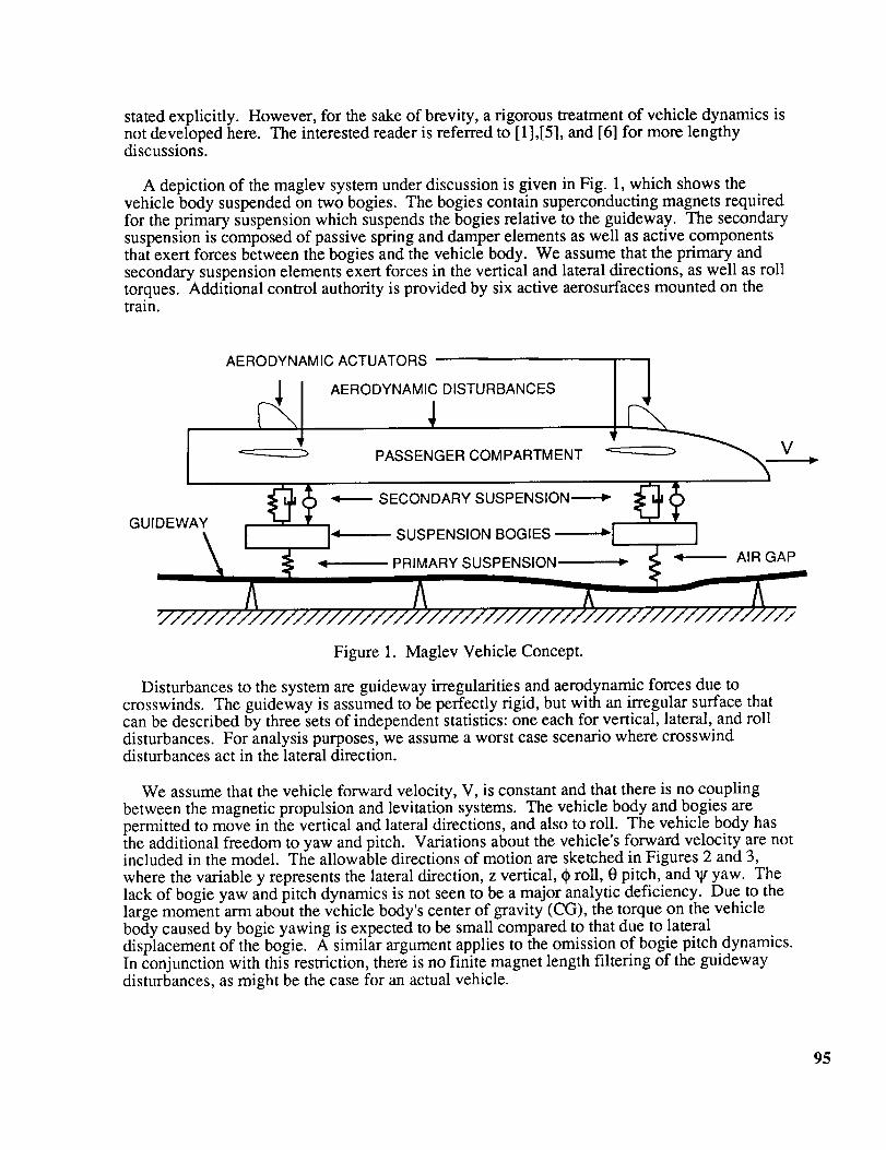
A depiction of the maglev system under discussion is given in Fig. 1, which shows thevehicle body suspended on two bogies. The bogies contain superconducting magnets requiredfor the primary suspension which suspends the bogies relative to the guideway. The secondarysuspension is composed of passive spring and damper elements as well as active componentsthat exert forces between the bogies and the vehicle body. We assume that the primary andsecondary suspension elements exert forces in the vertical and lateral directions, as well as rolltorques. Additional control authority is provided by six active aerosurfaces mounted on thetrain.

AERODYNAMIC ACTUATORS

AERODYNAMIC3[ DISTURBANCES _ V.___PASSENGER COMPARTMENT

SECONDARY SUSPENSION-_-_ _'__ T

I_ SUSPENSION BOGIES ;I IPRIMARY SUSPENSION _ _ AIR GAP

GUIDEWAY

Figure 1. Maglev Vehicle Concept.

Disturbances to the system are guideway irregularities and aerodynamic forces due tocrosswinds. The guideway is assumed to be perfectly rigid, but with an irregular surface thatcan be described by three sets of independent statistics: one each for vertical, lateral, and rolldisturbances. For analysis purposes, we assume a worst case scenario where crosswinddisturbances act in the lateral direction.

We assume that the vehicle forward velocity, V, is constant and that there is no couplingbetween the magnetic propulsion and levitation systems. The vehicle body and bogies arepermitted to move in the vertical and lateral directions, and also to roll. The vehicle body hasthe additional freedom to yaw and pitch. Variations about the vehicle's forward velocity are notincluded in the model. The allowable directions of motion are sketched in Figures 2 and 3,

where the variable y represents the lateral direction, z vertical, ¢ roll, 0 pitch, and _g yaw. Thelack of bogie yaw and pitch dynamics is not seen to be a major analytic deficiency. Due to thelarge moment arm about the vehicle body's center of gravity (CG), the torque on the vehiclebody caused by bogie yawing is expected to be small compared to that due to lateraldisplacement of the bogie. A similar argument applies to the omission of bogie pitch dynamics.In conjunction with this restriction, there is no finite magnet length filtering of the guidewaydisturbances, as might be the case for an actual vehicle.

95

The following additional assumptions are made: the vehicle body's and bogies' CGs are inthe geometric center of the respective bodies, both laterally and longitudinally; the vehicle bodyand bogies are completely rigid; the passengers and their baggage are fixed to the vehicle body;both bogies have identical dimensions, mass properties, and primary suspension stiffnesses; andsmall angle approximations are valid throughout the linear suspension model when relatinglinear to angular displacements.

The maglev vehicle's physical parameter values in our analyses are similar to a box-bearh

guideway design developed by the Bechtel consortium for the U.S. Department ofTransportation [ 1]. Representative gross physical properties are summarized in Table 1. Theremainder of this section consists of a brief synopsis of the suspension force models followedby a discussion of the active aerodynamic surfaces considered. The section is concluded withdescriptions of the guideway and crosswind disturbance models utilized.

A. Suspension Forces

To obtain a suitable linear system description, we model the maglev vehicle in a lumpedmass fashion. All suspension elements are modeled as massless generalized springs. Forexample, the suspension force, F, due to the displacement between the front bogie and theguideway is determined by the relationship below:

F = Kr + Df (1)

where K is the spring stiffness matrix, D is the damping, and r is the equilibrium displacementvector. The spring constants for the primary suspension system are dependent upon forwardvelocity; representative values as a function of train speed are given in Table 2. Damping forthis type of magnetic suspension is believed to be very low [7] and therefore is assumed zerofor modeling purposes. Passive secondary suspension spring constants and damping ratios areselected to improve ride quality while simultaneously preventing touchdown and limiting theactive secondary suspension stroke. The optimization procedure is discussed in §3.

96

Zvehicle LC _

Zrear bogie

)guideway

guideway

Zfront bogie

Z1 (t)gu_

guideway

Figure 2. Degrees of Freedom: Side View

vehicle

_.....---"'"_F -'_ Ybogie

Zguidewa___ Yguideway *guideway

[Guideway ] (__

Figure 3. Degrees of Freedom: Front View.

Table1RepresentativePhysicalDimensions

Parameter

Vehicle Height

Vehicle LengthVehicle Width

Total Mass

Passenger CompartmentMass

Distance Between Bogies

Bogie Height

Bogie WidthTop Winglet CP to TrainCG (vertical)

Side Winglet CP to TrainCG (horizontal)

Value

4.9m36.1m

3.7m

64400kg

40830kg

18.7m

0.75m

1.5m

2.3m

2.4m

Table 2

Primary Suspension Stiffness

Vehicle

Speed50.0m/s134.0

m/s150.0

m/s

ULateralStiffness

-1.09e7

N/m-1.35e7

N/m-1.36e7

N/m

VerticalStiffness

-3.23e7

N/m-3.97e7N/m

-4.01e7

N/m

It is assumed that all suspension forces act in equal and opposite directions across the gapbetween the elements under consideration. For simplicity, we model these forces as being

applied to fixed points relative to the guideway' s, bogies', and passenger compartment's centersof gravity.

B. Aerodynamic Actuation

Six active aerodynamic surfaces, as shown in Figure 1, are available to the control system forimproving ride quality. We assume that these actuators operate in "free-stream" and aremodeled as winglets with one degree-of-freedom. Four winglets are mounted on the sides ofthe train and produce vertical forces at the surfaces' centers of pressure (CP): two in front onopposite sides, and two in back on opposite sides. Two winglets are mounted on the top of thetrain (in "rudder-like" arrangements) to provide lateral forces.

The lift force for a flap in free-stream is given by:

FL = 1 pl Vai r 12AC L (_) (2)

where p is air density, A is area, Vair is the velocity of the air mass relative to the winglet, andoc represents angle of attack. We consider only the lift component of the flap forces. Theinduced drag of the flaps is calculated to determine the drawbacks of aerodynamic control in[5], but its effect on ride quality is not considered here. Since induced drag acts parallel to thevelocity vector, drag forces lie in a direction not included in our model. The lift coefficient isobtained from conventional aerodynamic theory [8] and is nearly linear for small angles ofattack. A linear equation for CL(Ot) results: CL(O0 = CL_, where CL = 0.0264/°. We assumethat Vair in (2) is equal to the train's velocity and ignore the effects of crosswind and vehiclerotation. Also, we use a small angle approximation for _ to model the lift force as

perpendicular to the undeflected winglet surface.

In theory, a very large aerodynamic force can be obtained for relatively low aero-actuatortorque. Since the flaps rotate about their centers of pressure, the aerodynamic torques across

97

flap rotation joints are small when compared to the forces generated by the flaps. However, theactual force required in a hydraulic system that drives a winglet can still be large, due tophysical constraints and practical considerations. The dynamics of the closed-loop system maydictate a high actuator bandwidth resulting in large actuator power requirements.

C. System Disturbances

Guideway irregularities are captured by the stochastic model:

ArV

_guideway (tO)= 0)2(3)

where Oguideway is the guideway Power Spectral Density (PSD), Ar is the Roughness

Parameter, and V is the train's forward velocity. A roughness parameter corresponding towelded steel rail (gage 4-6) is used to define the guideway PSD, which is subsequently used toform a linear system driven by white noise to describe the guideway position variations. Whilea typical guideway will not be made of steel and its irregularities as seen by the train will bedominated instead by the misalignment of guideway coils, its roughness parameters areexpected to fall in the range of those of welded steel rail. Roughness parameters are given inTable 3.

We assume further that the guideway disturbances act upon the front and rear of the train atthe bogie locations. Since the guideway is assumed rigid, the disturbance affecting the rearbogie is identical to that acting on the front bogie, but delayed in time. Therefore, we model therear guideway dynamics by the time delayed front guideway position variation. Clearly, thetime delay is inversely proportional to vehicle forward velocity: Tdelay = L/V, where L is thedistance between bogies. Since a time delay cannot be described by an exact finite dimensionalcontinuous time state space representation, a Pade approximation is incorporated into thecontrol system analysis and synthesis model:

2 + TdelayS + l__z__(_TdelayS) 2 + 1__(_TdelayS) 3 +...e-ST _ 2! 3! (4)

1 2 1 3

2 + TdelayS + -_._(TdelayS) + -_.i(TdelayS) +...

The crosswind description consists of the sum of two terms: a constant, steady-state meanvalue and a time variant random process. The mean crosswind velocity is equal to half of thepeak crosswind velocity, assuming a maximum three sigma variation from the mean. In ouranalysis we assume 26.8m/s (60mph) crosswind peak. The PSD of the time varying crosswindcomponent is given by:

2o_v

t_wind (0_) = C02 + V2 (5)

where the break frequency, v, is 1.0 rad/sec, and the RMS wind velocity, o w, is 4.8 m/s

(10mph). Owind is implemented by a linear system driven by white noise. We assume that the

crosswind is perpendicular to the guideway. This maximizes vehicle sideslip, effectivelysoftening the lateral suspension stiffness and thereby degrading system performance.

98

Table 3

Guideway Roughness Parameters

Parameter

Ar (vertical)

Ar (lateral)

Ar (roll)

Value

1.2e-6 rad^2-m/s

1.2e-6 rad^2-m/s

5.7e-7 rad^4/m-s

3. ANALYSIS

Analysis of the system model begins with choosing the passive secondary suspension'sstiffness and damping parameters. The function of the secondary suspension system is toimprove ride quality while simultaneously preventing vehicle contact (touchdown) on theguideway. The active secondary suspension stroke must also be kept within practical limits.Typically, the passive suspension parameters cannot be selected to optimize all of these criteriasimultaneously, and hence, the parameters are determined through trade-off analyses. Once thesuspension elements have been defined, a force balance condition is exploited to determinenominal operating equilibrium values for the vehicle's center of pressure and sideslip angle(given forward and average crosswind velocities). Finally, the linear perturbation model isassembled and a candidate control law synthesized. The resulting closed-loop system isanalyzed in a statistical framework. The remainder of this section presents further details ofthese procedures.

A. Secondary Suspension Parameter Optimization

The primary suspension design involves an inherent conflict between ride quality andguideway tracking. A stiff primary suspension provides improved guideway tracking at theexpense of significant guideway and wind disturbance transmission to the passengercompartment. Additionally, a stiff magnetic suspension generally exhibits efficient powerconsumption. Power considerations, rather than ride quality factors, generally dictate primarysuspenslon design. With the primary suspension parameters assumed given, the secondarysuspension parameters are chosen to address the trade-off between the system performancemeasures of interest, with the overall goal of achieving the best ride quality.

System performance can be evaluated through the root mean squared (RMS) values ofrelevant quantities in our model. RMS velocity and acceleration levels can be used to computethe Pepler index. The primary air gap and secondary suspension stroke requirements can alsobe estimated from the RMS variations of these variables, which provides a method ofspecifying the primary and secondary suspension stroke limits through stochastic controltechniques. The motivation behind this treatment stems from the guideway and winddisturbances being characterized by linear systems driven by white noise, whereby it is naturalto determine the system outputs for analysis in a similar form.

Details of the trade-off studies used for characterizing the passive secondary suspensionsystem are beyond the scope of this paper, but can be found in [1],[5], and [6]. The designparameter values are listed in Table 4.

99

Table4PassiveSecondarySuspensionParameters

Vertical NaturalFrequenc_¢Vertical Dampin_RatioLateralNaturalFrequencyLateralDampin[_RatioRoll StiffnessRoll Damping

0.8 Hz

0.101.5 Hz

0.5

0.0 N-m/rad

2.0e6 N-m-s/rad

B. Operating Point Force Balance

To obtain a linear state space perturbation analysis model, we need to determine the vehicle

steady-state sideslip angle, 13, and the location of the center of pressure (CP) relative to the CG.This is performed through a force balance analysis, where forces and moments arising from theconstant component of crosswind velocity are canceled by the primary and passive suspension

systems (Equation (1)). Crosswind forces on the train are modeled as a side force acting at theCP perpendicular to forward velocity. The aerodynamic side force is given by:

[Fy]aero = 1 plVair[2 mtCy (13)(6)

where At is the train's cross-sectional area and Cy(I3) is the coefficient of side force.. The air-relauve train velocity, Vair, is the vector sum of the train's earth-relative anct crosswlnavelocities. The aerodynamic coefficient, Cy(13), is non-linearly dependent on the sideslip angleand is described by a third order polynomial fit to data generated in [5].

Thus, given forward vehicle velocity and steady-state crosswind speed, the aerodynamicforces on the vehicle are computed as a function of 13and CP location via (6). A set of

nonlinear equations is solved numerically to determine 13and CP by balancing [Fy]aero againstthe nonaerodynamic forces contained in the model, where all time-varying zero meandisturbances and actuator displacements are nulled. For the data presented in §4, the vehicleand mean wind velocities are 150m/s (336mph) and 13.4m/s (30mph) respectively. The

resulting steady-state sideslip, 13,is 0.092rad (5.27°), which corresponds to a 0.0026rad (0.149 °)

vehicle yaw angle, _.

C. Covariance Analysis

To construct our linear perturbation model, we further assume that the passengercompartment and bogie angular rotation rates are small, and we neglect nonlinear couplingterms due to Coriolis accelerations and gyroscopic effects. The resulting linear equations ofmotion are placed in state space form, _k= Ax + Bu + Fw, where: the system state, x, containstrain and bogie positions and velocities, and guideway positions (constrained to appropriate

degrees of freedom); the system actuator input vector, u, contains active secondary suspensionforce and aerosurface deflection commands; and the disturbance input vector, w, is (Gaussian)

unit intensity white noise.

100

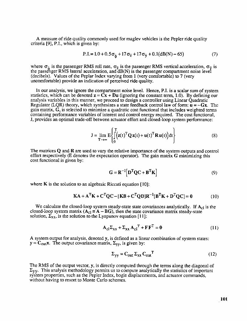
A measureof ride quality commonly used for maglev vehicles is the Pepler ride qualitycriteria [9], P.I., which is given by:

P.I.= 1.0 + 0.5 or+ + 17 _ + 17_ + 0.1 (dB(N) - 65) (7)

where o_is the passenger RMS roll rate, _ is the passenger RMS vertical acceleration, _ isthe passenger RMS lateral acceleration, and dB(N) is the passenger compartment noise level(decibels). Values of the Peplar Index varying from 1 (very comfortable) to 7 (veryuncomfortable) provide an indication of perceived ride quality.

In our analysis, we ignore the compartment noise level. Hence, P.I. is a scalar sum of systemstatistics, which can be denoted z = Cx + Du (ignoring the constant term, 1.0). By defining ouranalysis variables in this manner, we proceed to design a controller using Linear QuadraticRegulator (LQR) theory, which synthesizes a state feedback control law of form: u = -Gx. Thegain matrix, G, is selected to minimize a quadratic cost functional that includes weighted termscontaining performance variables of interest and control energy required. The cost functional,J, provides an optimal trade-off between actuator effort and closed-loop system performance:

J= lim E z(t)TQz(t)+u(t)TRu(t) dtT--+,=

(8)

The matrices Q and R are used to vary the relative importance of the system outputs and controleffort respectively (E denotes the expectation operator). The gain matrix G minimizing thiscost functional is given by:

G = R-I[DTQC + BTK] (9)

where K is the solution to an algebraic Riccati equation [10]:

KA + ATK + cTQc- [KB + CTQD]R-I[BTK + DTQc] = 0 (10)

We calculate the closed-loop system steady-state state covariances analytically. If Acl is theclosed-loop system matrix (Acl -- A - BG), then the state covariance matrix steady-statesolution, Zxx, is the solution to the Lyapunov equation [11]:

AclZxx + ]gxx Acl T + FFT = 0 (11)

A system output for analysis, denoted y, is defined as a linear combination of system states:

y = CoutX. The output covariance matrix, Zyy, is given by:

]_yy = Gout ]_xx Cout T (12)

The RMS of the output vector, y, is directly computed through the terms along the diagonal ofZyy. This analysis methodology permits us to compute analytically the statistics of importantsystem properties, such as the Pepler Index, bogie displacements, and actuator commands,without having to resort to Monte Carlo schemes.

101

4. RESULTS

Results obtained using the analysis model described in §2 are presented here. Controlalgorithms are developed and the resulting closed-loop systems analyzed as per §3. We selectthe weighting matrices, Q and R in (8), to provide good ride quality while maintaining, ifpossible, the strict suspension gap requirements defined in [1]. Tables 5 through 8 p.resent dataindicating basic system performance for four candidate control strategies: (1) no active control(open-loop); (2) active secondary suspension control only; (3) active aerosurfaces only, and (4)active secondary suspension and aerosurfaces (hybrid control). The tables present resultsassociated with guideway disturbances alone, crosswind disturbances alone, and the combinationof both sets of disturbances. RMS accelerations are evaluated for passengers seated over the

front bogie, at the center of the passenger compartment, and over the rear bogie. These RMSvalues, along with the RMS roll rate, permit ride quality to be evaluated in terms of the PeplerIndex at these three locations.

We assume a forward vehicle velocity of 150m/s (336mph) and a peak crosswind (three-

sigma) velocity of 26.8m/s (60mph). The nominal air ga.ps are 5 cm in the lateral direction and10 cm in the vertical direction. We desire a five-sigma air gap variation requirement in response

to disturbances. This requirement is most difficult to meet at the front of the vehicle, where thesteady-sate air gap deviation is 0.85 cm in the lateral and 0.72 cm in vertical direction. For thesecondary suspension strokes, the maximum allowable values are 19 cm in the lateral and 10 cmin the vertical direction, and in this case the requirement is relaxed to three-sigma variations.

Again, the front of the vehicle has the largest steady-state deviation, 3.19 cm in the lateraldirection and 2.43 cm in the vertical direction. Both the air gap variations and secondary

suspension strokes are determined at the outside edge of the front and rear bogies.

A. Passive Secondary Suspension

Passive secondary suspension optimization was described in §2. The performance given bythe passive system is given in Tables 5 through 8, and is taken as the baseline against which theactively controlled systems are compared. The ride quality, as measured by the Pepler index, isuncomfortable at the front and is tending toward somewhat uncomfortable at the center and rearof the vehicle. The acceleration, air gap, and secondary suspension stroke variations in thelateral direction are all largest at the front of the vehicle due to the location of the center of

aerodynamic pressure ahead of the center of gravity. The requirement on the lateral air gapvariations is not achievable for any secondary suspension design, and therefore indicates that abasic change in the primary suspension system is necessary. However, for the purposes of thispaper, the lateral air gap variations will be minimized as much as possible. Also, although notunreasonable, the 26.8m/s (60mph) peak crosswind velocity assumed for this study is rather

high; crosswinds of this level may not be present in all scenarios. However, since the crosswindforce is approximately proportional to the product of vehicle velocity and crosswind velocity, aspeed restriction during high wind conditions will ameliorate the detrimental effects ofcrosswinds.

B. Active Secondary Suspension

In this paper, active secondary suspension refers to a configuration where active hydraulicactuators are employed between the vehicle body and the bogies. The active and passive

suspension elements are assumed collocated. Note that the RMS acceleration levels for this

102

system have been reduced when compared to the passive system in both the vertical and lateral

directions. Since the passive system has vertical air gap variations which are below the systemrequirement, the optimal control design methodology was used to achieve smaller verticalaccelerations at the expense of larger air gap variations, as discussed in {}3. However, in thelateral direction, the passive design exhibited air gap variations which were larger than allowable

and so this trade-off could not be utilized. In addition, the authors decided that the control designshould not attempt to reduce the lateral air gap variations (relative to those achievable by passivesuspension); we do not endorse an EDS vehicle design that depends on the active control systemto maintain adequate air gap clearance. A failure of the control system could result in vehiclecontact with the guideway.

An important accomplishment of the active secondary suspension is the reduction of thevehicle roll rate by approximately a factor of 10. This is especially significant since roll has beenjudged to be an especially uncomfortable motion by passengers: half of the roll rate RMS addsdirectly to the Pepler index. The Pepler index has been reduced by 2.0-2.5 at all three locationsalong the vehicle. This results in a ride quality which is considered better than average andtowards comfortable at the center and rear.

A fundamental disadvantage of the active hydraulic actuators is that any force exerted againstthe vehicle body to cancel a disturbance will have an equal and opposite reaction force actingagainst the bogies. Thus there is a direct trade-off between air gap variations, secondarysuspension strokes, and vehicle accelerations.

C. Active Aerodynamic Surfaces

The use of active aerodynamic control surfaces results in vertical accelerations which aresmaller at all three locations along the vehicle and lateral accelerations which are lower at the

center and rear but slightly higher at the front of the vehicle. The ride quality (as measured bythe Pepler index) is the same at the front but slightly lower at the center and rear of the vehiclewhen compared to the active secondary suspension design. It is important to note that this ridequality improvement is obtained without any appreciable increase in the air gap variations, incontrast to the active hydraulic actuator suspension. Compared to the passive system, thesecondary suspension strokes are larger, especially in the vertical direction, but remain within

acceptable values. The roll rate is slightly less than that of the system with hydraulic actuators.

The primary advantage of the active aerodynamic surfaces is that they exert forces against thevehicle body with respect to an earth fixed (inertial) frame. Therefore, the effects of guidewaydisturbances on the vehicle body can be minimized without directly affecting the air gapvariations. This is equivalent to holding the vehicle body stationary" while the bogies bouncebeneath it. Of course, this results in larger secondary suspension stroke variations, as illustratedby the data presented. The crosswind forces cannot be canceled directly even though, like theaerodynamic control surfaces, they act directly on the vehicle body. Two primary reasons forthis arise because the crosswind disturbance is neither: (1) known beforehand, as the rearguideway disturbances are, nor (2) directly measurable. Another reason stems from non-collocation of crosswind forces and aerodynamic actuators.

The maximum RMS angle of attack of the aerodynamic surfaces was assumed to be 9 °, basedon the predicted deflection at which the aerodynamic surface stalls. This value was used for all

of the aerodynamic surfaces. More control authority for the lateral fin at the front of the vehiclewould have provided a greater potential for ride quality improvement. However, the size of theaerodynamic actuators at all locations was limited to practical values.

103

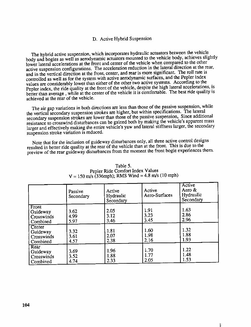
D. ActiveHybrid Suspension

Thehybrid activesuspension,which incorporateshydraulicactuatorsbetweenthevehiclebodyandbogiesaswell asaerodynamicactuatorsmountedto thevehiclebody,achievesslightlylower lateralaccelerationsat thefront andcenterof thevehiclewhencomparedto theotheractivesuspensionconfigurations.Theaccelerationreductionin the lateraldirectionattherear,andin theverticaldirectionatthefront, center,andrearis moresignificant. Theroll rateiscontrolledaswell asfor thesystemwith activeaerodynamicsurfaces,andthePeplerindexvaluesareconsiderablylower thaneitherof theothertwo activesystems.Accordingto thePeplerindex,theridequality at thefront of thevehicle,despitethehigh lateralaccelerations,isbetterthanaverage,while at thecenterof thevehicleit is comfortable.Thebestridequality isachievedat therearof thevehicle.

Theair gapvariationsin bothdirectionsarelessthanthoseof thepassivesuspension,whiletheverticalsecondarysuspensionstrokesarehigher,butwithin specifications.Thelateralsecondarysuspensionstrokesarelower thanthoseof thepassivesuspension,Sinceadditionalresistanceto crosswinddisturbancescanbegainedbothby makingthevehicle'sapparentmasslargerandeffectivelymakingtheentirevehicle'syawandlateralstiffnesslarger,thesecondarysuspensionstrokevariationis reduced.

Note thatfor the inclusionof guidewaydisturbancesonly, all threeactivecontroldesignsresultedin betterride quality attherearof thevehiclethanatthefront. This is dueto thepreviewof therearguidewaydisturbancesfrom themomentthefront bogieexperiencesthem.

Front

GuidewayCrosswindsCombinedCenter

GuidewayCrosswindsCombined

Rear

GuidewayCrosswindsCombined

Table 5.

Pepler Ride Comfort Index ValuesV = 150 m/s (336mph); RMS Wind -- 4.8 rn/s (10 mph)

Passive Active

Secondary HydraulicSecondary

3.62 2.054.99 3.125.97 3.46

3.323.614.57

3.693.524.74

1.812.072.38

1.961.882.33

ActiveAero-Surfaces

1.913.233.45

1.601.982.16

1.701.772.05

ActiveAero &

Hydraulic

Secondary

1.632.862.96

1.321.881.93

1.221.481.53

104

FrontY TrainAccelsGuidewayCrosswindsCombinedCenterYTrainAccelsGuidewayCrosswindsCombinedRearYTrainAccelsGuidewayCrosswindsCombinedFrontZTrainAccelsGuidewayCrosswindsCombinedCenterZTrainAccelsGuidewayCrosswindsCombinedRearZTrain AccelsGuidewayCrosswindsCombinedRoll RateGuidewayCrosswindsCombined

Table6.RMSVehicleAccelerationsandRoll Rate

V = 150rn/s(336mph);RMSWind = 4.8m/s (10mph)

PassiveSecondary

5.32g/lO014.26g/10015.22_/100

ActiveHydraulicSecondary

4.09g/lO011.09g/lO011.82_/100

3.89g/lO06.19g/lO07.31_/100

5.91g/lO05.62g/1008.16_100

6.38g/1003.62g/1007.34_/100

6.01g/1003.62g/1007.02g/lO0

6.19g/lO03.62g/lO07.17g,/1O0

1.27°/s1.89°/s2.28°/s

2.94g/lO04.94g/lO05.75g,/lO0

3.65g/lO03.84g/lO05.29_100

1.76 g/lO00.71 g/lO0

1.90 g,/lO0

1.50 g/lO00.71 g/lO0

1.66 _/lO0

1.67 g/lO00.71 g/lO0

1.81 _100

0.11 °/s0.22 °/s0.25 °/s

ActiveAero-Surfaces

4.08 g/10012.00 g/100

12.68 _/100

2.51 g/lO04.63 g/lO0

5.27 _100

2.93 g/lO03.38 g/lO0

4.48 _/100

1.04 g]lO00.62 g/lO01.21 _100

0.83 g]lO00.62 g/lO0

1.03 _100

0.99 g/1000.62 g/100

1.17 g]lO0

0.07 "/s0.17 °/s0.19 °/s

ActiveAero &

Hydraulic

Secondary

3.23 g/lO09.81 g/lO0

10.33 fllO0

1.42 g/lO04.05 g/lO0

4.29 ill00

0.81 g/lO01.73 g/lO0

1.91 _/100

0.33 g/lO00.61 g/lO0

0.69 g/lO0

0.30 g/lO00.61 g/lO0

0.67 _100

0.27 g/lO00.61 g/lO0

0.67 _100

0.06 °/s0.17 °/s0.18 °/s

105

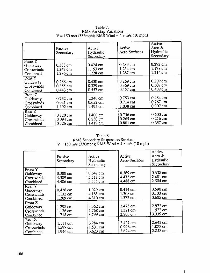
Table7.RMSAir GapVariations

V = 150m/s (336mph);RMSWind = 4.8rn/s(10mph)

Front YGuidewayCrosswindsCombinedRearYGuidewayCrosswindsCombinedFrontZGuidewayCrosswindsCombinedRearZGuidewayCrosswindsCombined

PassiveSecondary

0.333cm1.242cm1.286cm

0.266cm0.355cm0.443cm

0.732cm0.941cm1.192cm

0.720cm0.094cm0.726cm

ActiveHydraulicSecondar_

0.424cm1.153cm1.228cm

ActiveAero-Surfaces

0.289cm1.254cm1.287cm

0.450cm 0.2690.329cm 0.3690.557cm 0.457

1.346cm0.652cm1.495cm

1.400cm0.230cm1.419cm

cmcmcm

0.753cm0.714cm1.038cm

0.756cm0.265cm0.801cm

ActiveAero &HydraulicSecondary

0.292cm1.178cm1.214cm

0.269cm0.307cm0.409cm

0.484cm0.767cm0.907cm

0.600cm0.216cm0.637cm

Table8.RMSSecondarySuspensionStrokes

V = 150m/s (336mph);RMSWind = 4.8m/s (10mph)

Front YGuidewayCrosswindsCombinedRearYGuidewayCrosswindsCombinedFront ZGuidewayCrosswindsCombinedRearZGuidewayCrosswindsCombined

PassiveSecondary

0.380cm4.389cm4.406cm

0.426cm1.132cm1.209cm

1.298cm1.126cm1.718cm

1.111cm1.598cm1.946cm

ActiveHydraulicSecondary

0.642cm5.518cm5.555cm

ActiveAero-Surfaces

0.369cm4.473cm4.488cm

1.029cm 0.4144.185cm 1.3084.310cm 1.372

cmcmcm

2.475cm1.321cm2.805cm

3.362cm1.768cm3.799cm

3.284cm1.531cm3.623cm

2.427cm0.996cm2.624cm

ActiveAero &

Hydraulic

Secondary

0.338 cm2.481 cm2.504 cm

0.590 cm0.133 cm0.605 cm

2.972 cm1.522 cm3.339 cm

2.643 cm1.088 cm2.858 cm

106

5. CONCLUDING REMARKS

To analyze and quantify the benefits of active control, the authors have developed a fivedegree-of-freedom lumped parameter modeling capability suitable for a broad class of maglevvehicle and guideway configurations. Perturbation analyses about an operating point definedby train and average cross-wind velocities yield linearized state-space descriptions of themaglev system for multivariable control system analysis and synthesis. Results presented in §4indicate that the use of active aerodynamic control surfaces, in coordination with the active

secondary suspension system, provides significant improvement to the passenger ride qualitywhile ameliorating primary suspension gap requirements. Similar results by the authors ([1],[5], and [6]) for alternative system configurations support this conclusion.

Our analysis and design methodology permits us to alter physical properties, actuation (andpotentially, sensing) elements, and disturbance inputs contained within the linear modeldescription. This can be exploited to ascertain optimal system design parameters throughparametric trade-off analyses. (We appreciate that specific performance predictions generatedby linear analyses should ultimately be verified through high fidelity nonlinear simulation.) Anatural extension to our work includes appending additional modeling capabilities, e.g.: curvedand rolling guideways, vehicle bending modes, actuator and sensor dynamics and noise, and, ofcourse, more sophisticated control techniques.

REFERENCES

[10]

[11]

[1] Maglev System Concept Definition, contract DTFR 53-92-C-00003, prepared byBechtel/Draper/MIT/Hughes/General Motors for U.S. DOT: FRA.

[2] Wormley, D.N., Young, J.W., "Optimization of Linear Vehicle Suspensions Subjected toSimultaneous Guideway and External Force Disturbances," Journal of Dynamic Systems,Measurement, and Control: Transactions of the ASME, Paper No. 73-Aut-H, March16,1973.

[3] Guenther, Christian R., Leonides, Cornelius T., "Synthesis of a High-Speed TrackedVehicle Suspension System - Part I: Problem Statement, Suspension Structure, and

Decomposition," IEEE Transactions on Automatic Control, vol. AC-22, No. 2, April 1977.[4] Gottzein, E.; Lange, B., Ossenberg-Franzes, F., "Control System Concept for a Passenger

Carrying Maglev Vehicle," High Speed Ground Transportation Journal, Vol 9, No. 1,1975, pp 435-447.

[5] Barrows, T., McCallum, D, Mark, S, and Castellino, R. C, Aerodynamic Forces on

Maglev Vehicles, contract DOT/FRA/NMI-92/21, prepared by C.S. Draper Lab. for U.SDepartment of Transportation: Federal Railroad Administration.

[6] Mark, Steve, Modeling and Control of Maglev Vehicles. Masters Thesis, MITDepartment of Mechanical Engineering, 1993.

[7] Thornton, Richard D., "Magnetic Levitation and Propulsion, 1975," IEEE Transactions onMagnetics, Vol. Mag-11, No. 4, July 1975.

[8] Borst. H.V.; Hoerner, S.F., "Fluid-Dynamic Lift," published by Mrs Liselotte Hoerner,Bricktown, NJ, 1975.

[9] Dunlap and Associates, Inc., Development of Techniques and Data for Evaluating RideQuality Volume H: Ride Quality Research, Report No. DOT-TSC-RSPD-77-1, II forU.S. Dept. of Transportation, February, 1978.

Kwakernaak, H., and Sivan, R., Linear Optimal Control Systems. New York: Wiley-Interscience, 1972.

Jazwinski, A., Stochastic Processes and Filtering Theory. New York: Academic Press,Inc., 1970.

107

, , /

C

Session 4 - Superconductivity

Chairman: Nelson J. Groom

NASA Langley Research Center

109