N94- 35055

Accurate Estimation of Object Location in an Image Sequence

Using Helicopter Flight Data t

Yuan-Liang Tang and Rangachar Kasturi 2

Department of Computer Science and Engineering

The Pennsylvania State University

University Park, PA 16802

Phone: (814) 863-4254

Email: kasturi@cse.psu.edu

Abstract

In autonomous navigation, it is essential

to obtain a three-dimensional (3D) descrip-

tion of the static environment in which the

vehicle is traveling. For rotorcrafts con-

ducting low-altitude flight, this description

is particularly useful for obstacle detection

and avoidance. In this paper, we address

the problem of 3D position estimation for

static objects from a monocular sequence of

images captured from a low-altitude flying

helicopter. Since the environment is static,

it is well known that the optical flow in the

image will produce a radiating pattern from

the focus of expansion. We propose a mo-

tion analysis system which utilizes the

epipolar constraint to accurately estimate

3D positions of scene objects in a real world

image sequence taken from a low-aln'tude

flying helicopter. Results show that this ap-

proach gives good estimates of object posi-

tions near the rotorcraft's intended flight-path.

1 Introduction

To relieve the heavy workload imposed

upon the pilots, there is a need for automatic

obstacle detection systems onboard rotor-

crafts. The success of the system depends

upon the ability to accurately estimate object

positions near the rotorcraft's flightpath.

Several approaches for obstacle detection

and range estimation have been investigated

at NASA Ames Research Center [Bhanu89,

Cheng91, Roberts91, Smith92, Sridhar89].

In this paper, we propose an approach for

object position estimation using known cam-

era location and motion parameters.

For a rotorcraft with inertial-guidance

systems, the information about camera state

is continuously available as the rotorcraft

moves. This information can thus be used to

facilitate the processes of motion estimation

and scene reconstruction. For example, the

location of the focus of expansion (FOE) in

the image plane can be readily determined.

In addition, we assume the image acquisition

rate is high enough that an image feature will

not move by more than a few pixels in the

next image frame. Such closely sampled im-

ages will minimize the correspondence

problem between successive images. The

forward moving camera situation is the

worst case in depth estimation because the

optical flow in the image is small comparedto other motion cases. We overcome this

IThis research is supported by a grant from NASA Langley Research Center, Hampton, Virginia (NAG-l-1371).2Address all correspondence to Professor Kasturi.

147

https://ntrs.nasa.gov/search.jsp?R=19940030549 2018-07-05T20:42:38+00:00Z

problem by integrating information over along sequenceof images. As imageframesare accumulated,the baseline betweenthecurrent frameand the first frame increases,which givesbetter motion estimates.Bakerand Bolles [Baker89, Bolles87] used theEpipolar Plane Image (EPI) Analysis for

motion analysis. In their approach, camera

moving path is known and linear. Therefore,

each image frame can be decomposed into a

set of epipolar lines. An epipolar plane im-

age can thus be created by collecting corre-

sponding epipolar lines in each image frame.

Furthermore, when the viewing direction is

orthogonal to the direction of motion, the

apparent motion track of a feature on the

EPI is a straight line and the motion analysis

becomes merely a line fitting process. For

forward linear camera motion, however, the

feature tracks will be hyperbolas and curve

fitting becomes necessary. Sawhney et. al.

[Sawhney93] have reported that curve fitting

is much more difficult and noisy, making this

approach less robust. Matthies et. al.

[Matthies89] built a framework which gives

depth estimates for every pixel in the image.

Kalman filtering is used to incrementally re-

fine the estimates. In their experiments also,

the side-viewing camera is assumed and the

camera motion is only translational in the

vertical direction. Under such conditions,

feature tracks will follow the vertical image

scan lines and feature matching becomes

simpler. In our situation, the problem of

general camera motion is dealt with. We

handle this by breaking the camera motion

path into piece-wise linear segments.

Through this process, the camera path de-

termined by two consecutive camera posi-

tions is approximated as a straight line.

Epipolar planes can thus be set up for each

pair of images and motion analysis is recur-

sively performed on each pair of image

frames.

Our algorithms were tested on the heli-

copter images provided by NASA Ames Re-

search Center [Smith90]. There are two se-

quences of images, namely the line and the

arc sequences. Each sequence consists of 90

image frames with size 512x512 pixels andeach frame contains a header information

which records the helicopter body and cam-

era positions and orientations, body and

camera motion parameters, camera parame-

ters, etc. Time stamps are projected directly

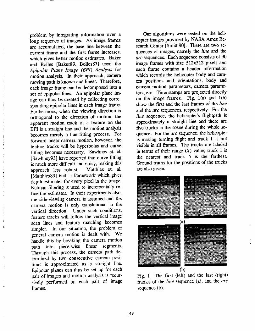
on the image frames. Fig. l(a) and l(b)

show the first and the last frames of the line

and the arc sequences, respectively. For the

line sequence, the helicopter's flightpath is

approximately a straight line and there are

five trucks in the scene during the whole se-

quence. For the arc sequence, the helicopter

is making turning flight and truck 1 is not

visible in all frames. The trucks are labeled

in terms of their range (X) value; truck 1 is

the nearest and truck 5 is the farthest.

Ground truths for the positions of the trucks

are also given.

(a)

(b)

Fig. 1 The first (left) and the last (right)

frames of the line sequence (a), and the arc

sequence (b).

148

Theremainingof this paper is organized

as follows. In Section 2, we describe how to

construct the epipolar lines. Section 3 dis-

cusses the feature extraction and tracking

processes. In Section 4, we present the

three-dimensional position estimation by

tracking outputs. Experimental results and

discussions are also given. Section 5 givesthe conclusion.

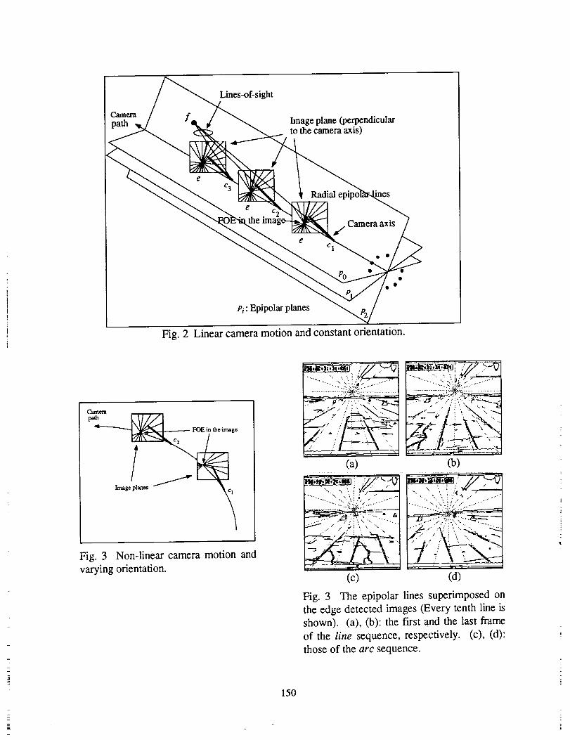
2 Constructing the Epipolar Lines

The epipolar constraint gives a strong

tool in confining the apparent motion direc-

tions of image features. In fact, the con-

strained directions are determined by epipo-

far planes as shown in Fig. 2(a), where all the

image frames share a common set of epipolar

planes. Since we are dealing with general

3D camera motion, the moving path of the

camera is not a straight line and its orienta-

tion is not constant during motion. Fig. 2(b)

illustrates such a case, where the camera's

path is an arc. Even if the camera is fixed on

the helicopter, its orientation is still changing

because the orientation of the helicopter

body is changing during nonlinear motion.

The location of the FOE also changes sig-

nificantly. In this case, there is no common

set of epipolar planes for all the image

frames. We solve this problem by using the

piece-wise linear approximation for the cam-

era path. Between two consecutive image

frames, the camera path is approximated as

linear and hence a pencil of epipolar planes

can be created in the 3D space which all in-

tersect at this segment of camera path. For

each pair of image frames, we first compute

the camera path parameters from the input

camera state data (positions and orienta-

tions). We then define a pencil of Q epipolar

planes, Pi, i=O .... Q-l, which all intersect at

the camera path. Q determines the resolu-

tion of the 3D space and hence the number

of features to be detected in the image. In

our experiments, Q is set to 100. The angle

between two adjacent epipolar planes Pi and

Pi+l is equal to n/Q. The result of this proc-

ess is the construction of a pencil of epipolar

planes equally spaced in terms of angular

orientations and they all intersect at the cam-

era path. After creating the epipolar planes,

epipolar lines on each image plane can thus

be determined by intersecting the image

plane and the epipolar planes. The process

of creating the epipolar lines is recursively

performed on each pair of image frames in

the sequence. Fig. 3 shows the epipolar lines

superimposed on the edge detected images.

The intersection of all the epipolar lines

shows the FOE. Even for the line sequence

in which the FOE is expected to remain at

the same pixel location in the image, it

changes by about 25 pixels both horizontally

and vertically. For the arc sequence, the

FOE location varies by about 70 pixels hori-

zontany and 30 pixels vertically.

3 Feature Detection and Tracking

The purpose of constructing epipolar

lines are two folds: to detect features and to

facilitate feature tracking. Features in an im-

age are defined to be the intersecting points

between the epipolar lines and the edge pix-

els detected by the Canny's edge detector

[Canny86]. The features are extracted from

the first image by tracing the pencil of

epipolar lines, Ii, i=O .... Q-1. The result will

be a number of Q sets of feature points and

feature detection and tracking on the follow-

ing frames are completely independent

among these sets. To obtain good localiza-

tion of detected features, the edges in the

image should be nearly perpendicular to the

epipolar lines.

149

Lines-of-sight

Image plane (perpendicularto the camera axis)

C 3

Radial ines

/ Camera axis

c I

Pi: Epipolar planes

Fig. 2 Linear camera motion and constant orientation.

path ["Tr77] FOE in the image

Image c_

Fig. 3 Non-linear camera motion and

varying orientation.

150

............... i:.:.:ii._.: ..ii..............

(a)=

(c)

(b)

'" " ... ",.'\ i i',-" ,"" ..........

(d)

Fig. 3 The epipolar lines superimposed on

the edge detected images (Every tenth line is

shown). (a), (b): the first and the last frame

of the line sequence, respectively. (c), (d):

those of the arc sequence.

Since we arc dealing with general camera

motion, the camera orientations for two

frames are likely to be different. Traditional

feature matchers try to search within the

neighborhood, i.e. the search window, of the

feature to be matched (the source feature).

With the information of camera state, we ar-

gue that this blindly positioning of the search

window is inappropriate because the term

neighborhood is incorrectly defined. The

following statement is one of the implicit as-

sumptions in defining the neighborhood tobe a window centered around the source

feature: "Since the image acquisition rate is

high enough such that the camera will not

move for a long distance between two con-

secutive frames, the source feature will not

move more than a few pixels in the next im-

age plane." We find this statement sustains

only if the camera orientation keeps approxi-

mately constant during the camera motion.

As is well known, even a small amount of

camera rotation can actually create large im-

age feature motion in the image plane.

Hence, the camera rotation has much more

influence on image feature motion compared

to camera translation, especially when thedistance from the camera to a world feature

is very large compared to the distance the

camera travels between two consecutive

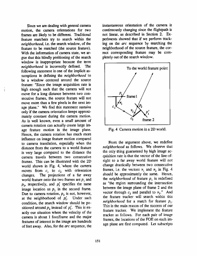
frames. This can be illustrated with the 2D

world shown in Fig. 4, where the camera

moves from ct to cz with orientation

changes. The projections of a far away

world feature onto the two frames are p, and

p_, respectively, and p_ specifies the same

image location as p_ in the second frame.

Due to camera rotation, Pz is not, however,

at the neighborhood of p[. Under such

condition, the search window should be po-

sitioned around Pz instead of p_. This is ex-

actly our situation where the velocity of the

camera is about 1 foot/frame and the major

features of interest in the image are hundreds

of feet away. Also, for the arc sequence, the

instantaneous orientation of the camera is

continuously changing since the flightpath is

not linear, as described in Section 2. Ex-

periments showed that if we perform track-

ing on the arc sequence by searching the

neighborhood of the source feature, the cor-

rect corresponding feature may be com-

pletely out of the search window.

To the world feature point

f_l/cz frame 2

Fig. 4 Camera motion in a 2D world.

From the argument above, we redefine

neighborhood as follows. We observe that

the only thing guaranteed by high image ac-

quisition rate is that the vector of the line-of-

sight to a far away world feature will not

change drastically between two consecutive

frames, i.e. the vectors v_ and vz in Fig. 4

should be approximately the same. Hence,

the neighborhood of feature p, is redefined

as "the region surrounding the intersection

between the image plane of frame 2 and the

vector through c2 and parallel to v_." Andthe feature tracker will search within this

neighborhood for a match for feature pt.This is the main reason of the success of our

feature tracker. We implement the feature

tracker as follows. For each pair of image

frames, the locations of the FOE on each im-

age plane are first computed. Let subscripts

151

1 and 2 denote the time instance of the first

and the second frame, respectively. For each

image feature at location p_ in the first frame

11, we first compute v x which is the 3D vec-

tor from the camera center c_ to p_. And

then, the hypothetical location Pz is obtained

by intersecting 12 with the vector v I passing

through camera center c2. Incorporating the

epipolar constraint, instead of searching

within a region centered around P2, the fea-ture_tracker follows the direction of the

epipolar line; which is determined by the

FOE and Pz. In our experiment, we use

seven pixels as the 1D window size. Feature

detection and tracking are then performed

within this window on the second image.

Note that, in order to reduce the amount of

computation we perform the feature detec-

tion and tracking based on the edge pixels

only. For more robust feature tracking, the

intensity distribution around a feature shouldbe considered.

Within a small 1D neighborhood, we

have a number of features (source features)

in the first image and a number of features

(target features) in the second image to be

matched. Depending on the matching re-

suits, a feature will be labeled as matched,

new, no match, and multiple matches:

1. Matched: There is only one target fea-

ture in the neighborhood. If there are

several source features which are compet-

ing for the target (i.e. the occlusion case),

the target will be matched to the source

feature which has a stable position esti'

mate. The position estimate of a feature

is considered stable if its estimated posi-

tion remains approximately the same

through several frames (see Section 4). If

more than one source feature have a sta-

ble position estimate, local slope of their

tracks is compared. Fig. 5(a) shows sucha situation. Source features A and B can

both match to target C. The track with

152

steeper slope (B) should correspond tothe feature which is more distant from the

camera than A. Since only the near fea-

ture can occlude the farther one, target Cwill be matched to feature A. For the

matched source feature, its image (2D)

position will be updated and its 3D posi-

tion estimated (described in Sectio n 4).Feat_ure B will be labeled no match and

handled as described later,

2. New: When a new feature appears in the

current image, it has no Source feature to

match. A feature node will be created and

inserted in the database.

3. No match: This may be due to the failure

of feature detector, occlusion, or feature

moving out of the image. For the last

case, which can be easily detected, the

source feature is simply removed. For the

other two cases, if the source feature al-

ready has a stable 3D position estimate,

the feature tracker will make a hypothesis

about its image position based on its 3D

position estimate. No estimation will be

performed on these features except for

updating their 2D position using the hy-

pothesis. For other features, since we

• have no reliable information about their

position, they remain in their current state

awaiting possible matches in the future. Amaximum number of consecutive no

matches is defined to remove those fea-

tures being occluded or missed by the de-

tector for a long time. _ :

4. Multiple matchesi In this-:ease; more

than one target feature appears within the

neighborhood. This may result from fea-

ture disocclusion or due to the noise from

the feature detector. The goal here is to

choose the best match. Cox [Cox93] re-

viewed some of the approaches including

nearest-neighbor [Crowley88], Maha-

lanobis distance [The_ien89], track-

splitting filter [Smith75], joint-likelihood

!i|

!i

!

=_

=_

!=

E

!

!

i

|

I

!

iE

j

E

Z

[Morefield77], etc. In our problem, since

the epipolar constraint already gives an ef-

fective means to improve the tracking

process, simple techniques are used to re-

solve this confusion and at the same time

reduce the algorithm complexity. This

idea is also supported by three observa-

tions. First, if the feature already has a

stable 3D position estimate, the best

match can be easily found by projecting its

position estimate onto the current image.

Second, according to the epipolar con-

straint, actually only one direction (away

from FOE) is possible for the feature mo-tion under noise-free circumstances.

Hence, the feature motion conforming this

constraint should be favored. And finally,

the size of the search window is small,

giving only a small number of multiple

matches. Hence, the matching problem is

simplified. With these observations, we

use the following three priority criteria for

choosing a feature to be the best match:

(1) the one which satisfies the position es-

timate; (2) the one which is in the direc-

tion away from the FOE and is nearest;

and (3) the one which is in the direction

towards the FOE and is nearest. The

main reason to include (3) as a legal

match is to compensate the feature detec-

tion noise. These three criteria will also

determine the weights in the position es-

timation (see Section 4). Fig. 5(b) gives a

demonstration of how complicated the

multiple match can be. Source feature A

in frame 2 is searching for a best match

among the target features in frame 3.

Correct track is AEFG, but feature E (the

blank circle) is missed by the detector.

There exist also disocclusions (squares

and triangles) and noise (star). Several

scenarios and consequences are possible

in our tracking process: (1) The tracker

chooses feature B (the triangle) as the best

match, feature A is already stable, and

feature F is detected and within B's search

window in frame 4. Since B does not

satisfy the estimated location of A, it will

be lightly weighted in the position estima-tion and has little contribution to the esti-

mate. However, according to the esti-

mated position, the tracker will pick the

correct match, feature F, as the best

match in frame 4. (2) The tracker

chooses feature B as the best match, fea-

ture A is stable, and feature F is not in B's

search window or is missed again. The

tracker will follow the track ABC, which

is wrong for feature A. The tracker, how-

ever, may still make correction on its

tracking if it is possible to match feature

G to feature C in frame 5. Otherwise it

will follow the path of the triangles and

the position estimates will gradually be-come unstable. Such features can be rec-

ognized by noting that their position esti-

mates are still unstable after lengthy

tracking. We then reset their estimatesand start a new estimate similar to that for

newly appeared features. (3) The trackerchooses B as the best match and feature A

has no stable estimates. The tracking will

either follow the circles or the triangles

depending on which one is nearer. This

does not matter too much since no reliable

information has been accumulated and

these errors will be lightly weighted in the

position estimation. (4) The tracker

chooses the noise (star) as the best match.

This will be similar to what has been dis-

cussed, i.e. the tracker may correct its

tracking if it is possible to pick feature F

in frame 4. Otherwise, the estimate will

be reset if track BCD is followed.

Feature matching is difficult and may

contribute to most of the error in image

analysis. From the analysis above, we can

see that the epipolar constraint helps to

simplify and to improve the matching quality.

The matcher may be further improved by in-

153

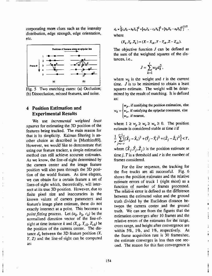
corporating more clues such as the intensity

distribution, edge strength, edge orientation,

etc.

.211/2

where

(x, .r,. z,) = (x - x a ,r - ra,z-

Frlr_ #

P_cs of f,,._tur,'-aloq m ep/polar line

i _ -

2 _ _ .A

4 --C _5 _

(a) co)

Fig. 5 Two matching cases: (a) Occlusion

(b) Disocclusion, missed features, and noise.

The objective function J can be defined as

the sum of the weighted squares of the dis-

tances, i.e.,l

J--Zk=l

where wk is the weight and t is the currenttime. J is to be minJmiz_ to obtain a least

squares estimate. The weight will be deter-

mined by the result of matching. It is defined

as:

4 Position Estimation and

Experimental Results

We use incremental weighted least

squares for estimating the 3D position of the

features being tracked. The main reason for

that is its simplicity. Kalman f'dtering is an-

other choice as described in [Matthies89].

However, we would like to demonstrate that

using our feature tracker, a simple estimation

method can still achieve accurate estimates.

As we know, the line-of-sight determined by

the camera center and the image feature

position will also pass through the 3D posi-

tion of the world feature. As time elapses,

we can obtain for a certain feature a set of

lines-of-sight which, theoretically, will inter-

sect at its true 3D position. However, due to

finite pixel size and inaccuracies in the

known values of camera parameters and

feature's image plane estimate, these do not

exactly intersect at a point. This becomes a

point fitting process. Let (a k, b k, ck) be thenormalized direction vector of the line-of-

sight at time instance k and (Xck, Yck, Zck) be

the position of the camera center. The dis-

tance dk between the 3D feature position (X,

Y, Z) and the line-of-sight can be computed

as:

wp, if sastifying the position estimation, else

wk = )we, if satisfying the epipolar constraint, else[w n, if nearest,

where 1 > wp > we > wn > O. The positionestimate is considered stable at time t if

t-1. ^

1 r,r.

j=t-r

where (Xj,Yj,Zj) is the position estimate at

time j, T is a threshold and r is the number of

flames considered.

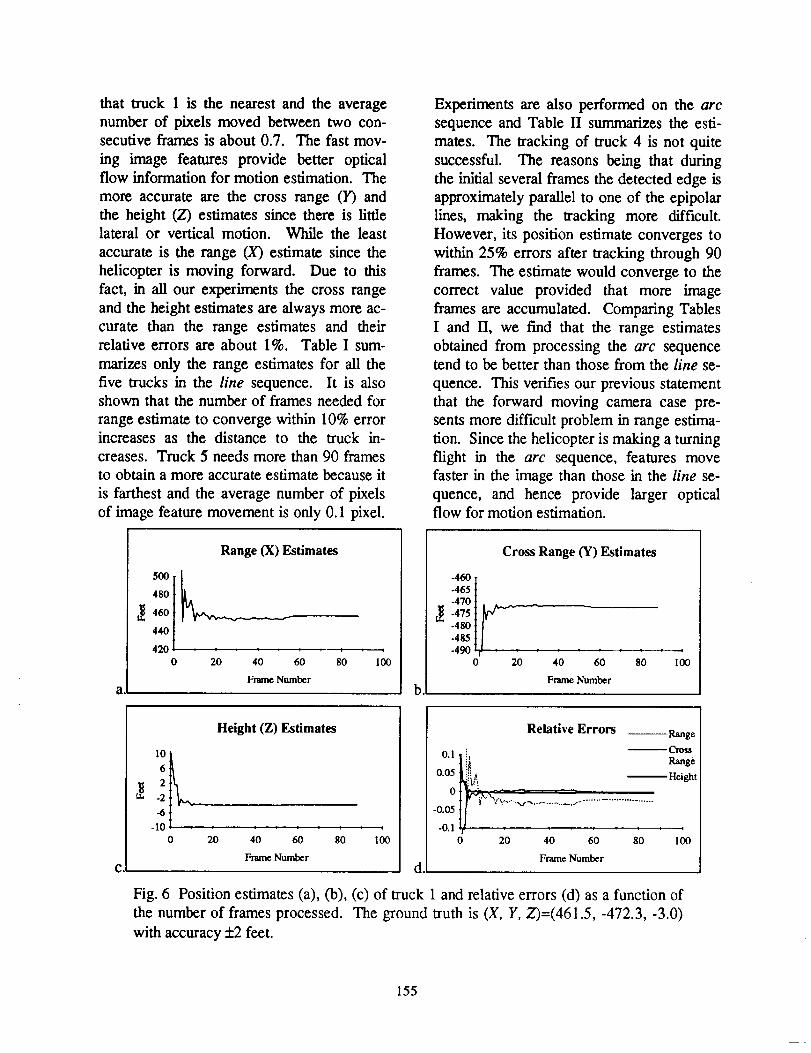
For the line sequence, the tracking for

the five trucks are all successful. Fig. 6

shows the position estimates and the relative

estimate errors of truck 1 (right most): as a

function of number of flames processed.The relative error is defined as the difference

between the estimated value and the ground

truth divided by the Euclidean distance be-

tween the camera center and the ground

truth. We can see from the figures that the

estimation converges after 10 frames and therelative errors of the estimates for the range,

cross range, and height after convergence are

within 5%, 1%, and 1%, respectively. As

the frame acquisition rate is 30 flames/see,

the estimate converges in less than one sec-

ond. The reason for this fast convergence is

154

that truck 1 is the nearest and the average

number of pixels moved between two con-secutive frames is about 0.7. The fast mov-

ing image features provide better optical

flow information for motion estimation. The

more accurate are the cross range (Y) and

the height (Z) estimates since there is little

lateral or vertical motion. While the least

accurate is the range (X) estimate since the

helicopter is moving forward. Due to this

fact, in all our experiments the cross range

and the height estimates are always more ac-

curate than the range estimates and their

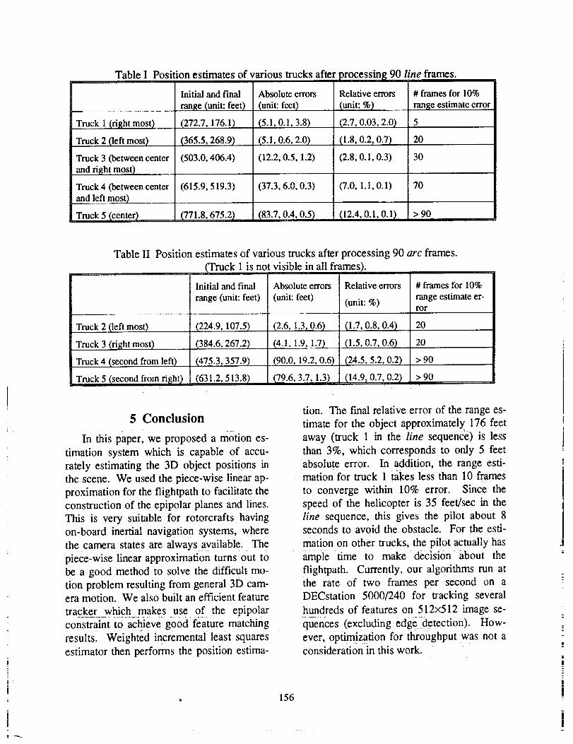
relative errors are about 1%. Table I sum-

marizes only the range estimates for all the

five trucks in the line sequence. It is alsoshown that the number of frames needed for

range estimate to converge within 10% errorincreases as the distance to the truck in-

creases. Truck 5 needs more than 90 frames

to obtain a more accurate estimate because it

is farthest and the average number of pixels

of image feature movement is only 0.1 pixel.

Experiments are also performed on the arc

sequence and Table II summarizes the esti-

mates. The tracking of truck 4 is not quite

successful. The reasons being that during

the initial several frames the detected edge is

approximately parallel to one of the epipolar

lines, making the tracking more difficult.

However, its position estimate converges to

within 25% errors after tracking through 90

frames. The estimate would converge to the

correct value provided that more image

frames are accumulated. Comparing Tables

I and II, we find that the range estimates

obtained from processing the arc sequencetend to be better than those from the line se-

quence. This verifies our previous statement

that the forward moving camera case pre-

sents more difficult problem in range estima-

tion. Since the helicopter is making a turning

flight in the arc sequence, features move

faster in the image than those in the line se-

quence, and hence provide larger opticalflow for motion estimation.

500 I480

440 I420 /

0

Range (X) Estimates

J ) J i i ! i i

20 40 60 80 100

Frame Number

Cross Range (Y) Estimates

-470 1.

-480 | |

-485t !-490 _ ......

0 20 40 60 80 I00

Frame Number

a, b,

Co

6

2

-2

-6

-10

0

Height (Z) Estimates

) : : : : : e i I

20 40 60 80 100

Frame Number

Relative Errors

o.1 i.

0.05 _.,_o I _',,'_',,,.,....... " '..........................

-0.05 !! '- . v... -.-.,, _-0.1

0 20 40 60 80

Frame Numberd

-- Range

Cross

Range

_Height

100

Fig. 6 Position estimates (a), (b), (c) of truck 1 and relative errors (d) as a function of

the number of frames processed. The ground truth is (X, Y, Z)=(461.5, -472.3, -3.0)

with accuracy _+_2feet.

155

TableI Position estimates of various trucks after

Truck 1 (right most)

Truck 2 (left most)

Truck 3 (between center

and right most)

Truck 4 (between center

and left mosQ

Truck 5 (center)

Initial and final

range (unit: feet)

(272.7, 176.1)

(365.52 268.9)

(503.0, 406.4)

(615.9, 519.3)

(771.8,675.2)

Absolute errors

(unit: feet)

(5.1,0.1,3.8)

(5.1, 0.6, 2.0)

(12.2, 0.5, 1.2)

(37.3, 6.0, 0.3)

(83.7, 0.4, 0.5)

Relative errors

(unit: %)

(2.7, 0.03, 2.0)

(1.8, 0.2, 0.7)

(2.8, O. 1, 0.3)

(7.0, 1.1, 0.1)

.... Q2.4, 0.1, 0.1)

?rocessing 90 line frames.

# frames for 10%

range estimate error

5

20

30

70

> 90

Table II Position estimates of various trucks after processing 90 arc frames.

(Truck 1 is not visible in all frames).

Truck 2 (left most)

Truck 3 (right most)

Truck 4 (second from left)

Truck 5 (second from right)

Initial and final

range (unit: feet)

(224.9, 107.5)

(384.6, 267..2)

(475.3, 357.9)

(631.2, 513.8)

Absolute errors

(unit: feet)

(2.6, !.3, 0_6)

(4.1, 1.9, !.7)

(90.0, 19.2, 0.6)

(79.6, 3.7, 1.3)

Relative errors

(unit: %)

(1.7, 0.8, 0.4)

(1.5, 0.7, 0.6)

# frames for 10%

range estimate er-ror

20

20

> 90

> 90

5 Conclusion

In this paper, we proposed a motion es-

timation system which is capable of accu-

rately estimating the 3D object positions in

the scene. We used the piece-wise linear ap-

proximation for the flightpath to facilitate the

construction of the epipolar planes and lines.

This is very suitable for rotorcrafts having

on-board inertial navigation systems, where

the camera states are always available. The

piece-wise linear approximation turns out to

be a good method to solve the difficult mo-

tion problem resulting from general 3D cam-

era motion. We also built an efficient feature

tracker which makes use of the epipolar

constraint to achieve good feature matching

results. Weighted incremental least squares

estimator then performs the position estima_

tion. The final relative error of the range es-

timate for the object approximately 176 feet

away (truck 1 in the line sequence) is less

than 3%, which corresponds to only 5 feet

absolute error. In addition, the range esti-

mation for truck 1 takes less than 10 frames

to converge within 10% error. Since the

speed of the helicopter is 35 feet/sec in the

line sequence, this gives the pilot about 8seconds to avoid the obstacle. For the esti-

mation on other trucks, the pilot actually has

ample time to make decision about the

flightpath. Currently, our algorithms run at

the rate of two frames per second on a

DECstation 5000/240 for tracking several

hundreds of features on 512x512 image se-

quences (excluding edge detection). How-

ever, optimization for throughput was not aconsideration in this work.

i

_ 156

ii

Reference

[Baker89] Baker, H.H. and R.C. Bolles,

"Generalizing Epipolar-Plane Image

Analysis on the Spatiotemporal Surface,"

Int. J. Computer Vision, Vol. 3, pp. 33-49, 1989.

[Bhanu89] Bhanu, B., B. Roberts, and J.C.

Ming, "Inertial Navigation Sensor Inte-

grated Motion Analysis," Proc. DARPA

Image Understanding Workshop, pp.

747-763, 1989.

[BoUes87] Bolles, R.C, H.H. Baker, and

D.H. Marimont, "Epipolar-Plane Image

Analysis: An Approach to DeterminingStructure from Motion," Int. J. Com-

puter Vision, Vol. 1, pp. 7-55, 1987.

[Canny86] Canny, J., "A Computational

Approach to Edge Detection," IEEE

Trans. Pattern Analysis and Machine

Intelligence, Vol. 8, No. 6, pp. 679--698,1986.

[Cheng91] Cheng, V.H.L. and B. Sridhar,

"Considerations for Automated Nap-of-

the-Earth Rotorcraft Flight," Journal of

the American Helicopter Society, Vol.

36, No. 2, pp. 61-69, 1991.

[Cox93] Cox, I.J., "A Review of Statistical

Data Association Techniques for Motion

Correspondence," Int. J. Computer Vi-

sion, Vol. 10, No. 1, pp. 53-66, 1993.

[Crowley88] Crowley, J.L., P. Stelmaszyk,

and C. Discours, "Measuring Image Flow

by Track Edge-lines," Proc. Int. Conf.

Computer Vision, pp. 658-664, 1988.

[Matthies89] Matthies, L., T. Kanade, and

R. Szeliski, "Kalman Filter-based Algo-

rithms for Estimating Depth from Image

Sequences," Int. J. Computer Vision,

Vol. 3, No. 3, pp. 209-236, 1989.

[Morefield77] Morefield, C.L., "Application

of 0-1 Integer Programming to Multitar-

get Tracking Problems," IEEE Trans.

Automatic Control, AC-22(6), 1977.

[Roberts91] Roberts, B., B. Sridhar, and B.

Bhanu, "Inertial Navigation Sensor Inte-

grated Motion Analysis for Obstacle

Detection," Digital Avionics Systems

Conference, pp. 131-136, 1991.

[Sawhney93] Sawhney, H.S., J. Oleinsis,

and A.R. Hanson, "Image Description

and 3-D Reconstruction from Image

Trajectories of Rotational Motion,"

IEEE Trans. Pattern Analysis and Ma-

chine Intelligence, Vol. 15, No. 9, pp.

885-898, 1993.

[Smith75] Smith, P. and G. Buechler, "A

Branching Algorithm for Discriminating

and Tracking Multiple Objects," IEEE

Trans. Automatic Control, AC-20: pp.

101-104, 1975.

[Smith90] Smith, P.N., "NASA Image Data

Base User's Guide," NASA Ames Re-

search Center, Moffett Field, CA., Ver-

sion 1.0, 1990.

[Smith92] Smith, P.N., B. Sridhar, and B.

Hussien, "Vision-Based Range Estima-

tion Using Helicopter Flight Data," IEEE

Conf. Computer Vision and Pattern

Recognition, pp. 202-208, 1992.

[Sridhar89] Sridhar, B., V.H.L. Cheng, and

A.V. Phatak, "Kalman Filter Based

Range Estimation for Autonomous

Navigation Using Imaging Sensors,"

Proc. llth IFAC Symposium on Auto-

matic Control in Aerospace, 1989.

[Therrien89] Therrien, C.W., Decision Es-

timation and Classification: An Intro-

duction to Pattern Recognition and Re-

lated Topics, Wiley, New York, 1989.

157

m

!

i

i

!

Image Processing and DataClassification

PI_ FAGE BLA_"iK NbT FFLMED

159

-A