Embed Size (px)
Citation preview
N89-13318
Absolute Photometric Calibration of Detectors to 0.3 mmag
Using
Amplitude-Stabilized Lasers
and
A Helium-Cooled Absolute Radiometer
Peter J. Miller
Cambridge Research and Instrumentation, Inc., Cambridge, MA
Short Title: Absolute Detector Calibration using Lasers and a Radiometer
PRECEDING PAO{_ {{LANK NOT PrLMED
153
https://ntrs.nasa.gov/search.jsp?R=19890003947 2020-03-31T19:54:14+00:00Z

Section I: Abstract
We describe laser sources whose intensity is determined with a
cryogenic electrical substitution radiometer. Detectors are then
calibrated against this known flux, with an overall error of 0.028%
(0.3 mmag). Ongoing research at C.R.I. has produced laser intensity
stabilizers with flicker and drift of < 0.01%. Recently, the useful
wavelength limit of these stabilizers has been extended to 1.65 mi-
crons by using a new modulator technology and InGaAs detectors. This
will allow improved characterization of infrared detector systems.
We compare data from a Si photodiode calibration using the method of
Zalewski and Geist against an absolute cavity radiometer calibration,
as an internal check on the calibration system.
Section 2: Introduction
Liquid helium cooled electrical substitution radiometers have been
developed in order to realize the higher accuracy, lower noise floor,
and faster time response which cryogenic operation provides I - 4.
Their high absolute accuracy has been demonstrated at the NPL through
direct measurement of the Stefan-Boltzmann constant, and by comparison
with emission from the BESSY source. The absolute error of these
devices is estimated at 0.01%. We have constructed a calibration
facility based upon a cryogenic absolute radiometer, whose optics have
been optimized for use with collimated laser sources. The radiometer
is discussed in Section 4.
In a laser-based calibration, the radiometer optics are greatly
simplified, with a corresponding increase in accuracy. In particular,
corrections for aperture size indeterminacy, for diffraction, for
154

scattered light, and for spectral variations are reduced to negligible
size (< i ppm). However, in order to realize the high accuracy which
a helium-cooled radiometer offers, the intensity of the laser source
must be stable to the samehigh degree. Accordingly, we have devel-
oped laser amplitude stabilizers which use feedback control techniques
to stabilize the intensity of laser sources to better than 0.01 per-
cent over one hour. Further, these stabilizers can now stabilize
infrared lasers, to wavelengths of at least 1.52 microns. They are
described in Section 3.
The overall calibration system is diagrammedin Figure I, and
consists of a bank of laser sources; a laser stabilizer; a detector
wheel which contains the device(s) to be calibrated; and the cryogenic
radiometer (see Figure I). In order to calibrate a detector at a
particular power level and wavelength, the appropriate laser is
selected and the rough power level selected by the use of neutral
density filters and adjustments to the laser itself. The beampasses
through a laser intensity stabilizer, which is used to select the
exact operating intensity level. A reading is then taken with the
device being calibrated.
Whenthe device response has been measured, the detector wheel is
rotated to let the beampass through to the cryogenic radiometer. A
reading of the beampower is then madeby the radiometer, which takes
approximately two minutes. The responsivity of the device is given by
the device response divided by the beampower, as determined by the
radiometer. If needed, a detector dark count reading can be made
while the beampower is being measuredby the radiometer; conversely,
the dark count reading required by the radiometer is madewhile the
155

detector response is being measured.
Note that this calibrates the detector's radiometric response, but
since a monochromatic source is used, a photometric calibration may be
easily derived from it. The two calibrations are related by the
energy per photon at the wavelength of calibration; since that wave-
length is known to 7 digits or more, there is no error suffered
through this practice. The calibration procedure and the system per-
formance are described in Section 5, following a detailed description
of the individual components.
Section 3: The stabilized laser source
Lasers are underutilized in the calibration world. Their high
specific radiance, monochromaticity, excellent beam profile, ease of
collimation, and ease of use recommend them for many photometric
measurements. However, they are intrinsically unstable in their power
output, exhibiting fluctuations of a few percent. Laser designers
seek to minimize these fluctuations, but their efforts are hampered by
the fact that lasers are designed to be runaway oscillators.
We have developed a commercial line of laser intensity stabilizers
which operate outside of the laser itself, based on work done at the
Bureau of Standards 5. Figure 2 is a block diagram of one of these
units. Light from the unstabilized laser passes through an input
polarizer, which linearly polarizes it. The light'then passes through
a Pockels" cell, which is a voltage-controlled waveplate. Depending
on the applied voltage, the polarization axis of the light is rotated
by an angle between 0 and 90 degrees. Next, the light passes through
a second, exit polarizer; the fraction of the light transmitted
156
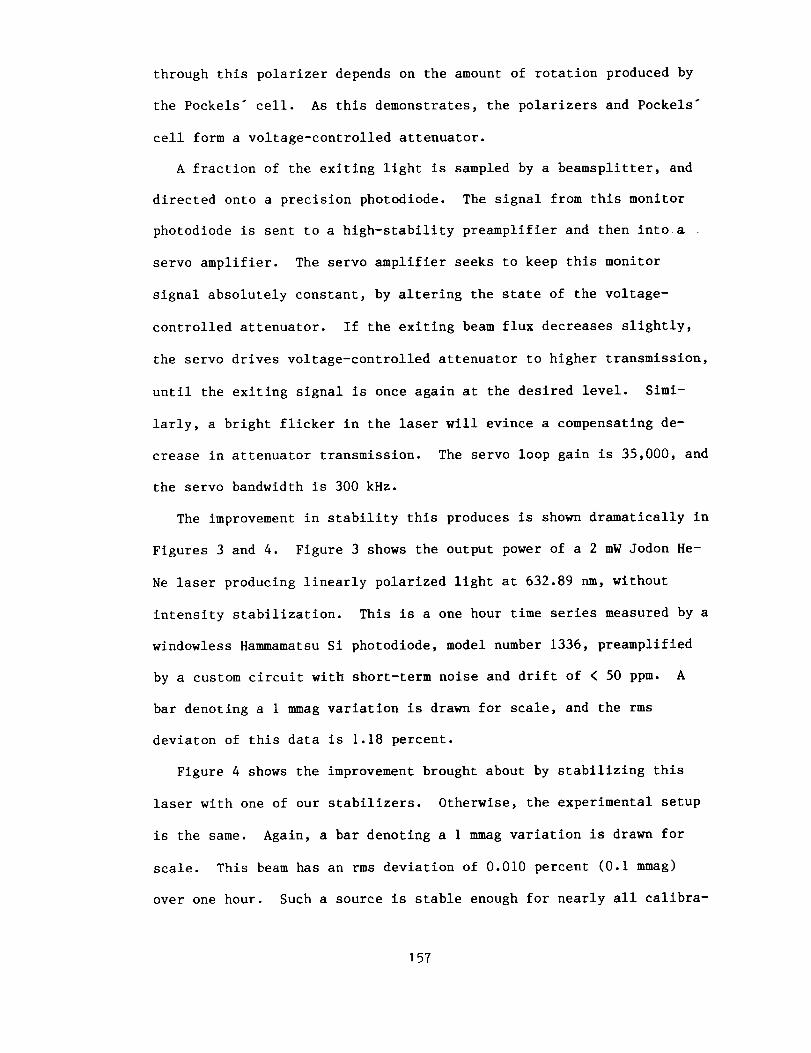
through this polarizer depends on the amount of rotation produced by
the Pockels" cell. As this demonstrates, the polarizers and Pockels"
cell form a voltage-controlled attenuator.
A fraction of the exiting light is sampled by a beamsplitter, and
directed onto a precision photodiode. The signal from this monitor
photodiode is sent to a high-stability preamplifier and then into a
servo amplifier. The servo amplifier seeks to keep this monitor
signal absolutely constant, by altering the state of the voltage-
controlled attenuator. If the exiting beam flux decreases slightly,
the servo drives voltage-controlled attenuator to higher transmission,
until the exiting signal is once again at the desired level. Simi-
larly, a bright flicker in the laser will evince a compensating de-
crease in attenuator transmission. The servo loop gain is 35,000, and
the servo bandwidth is 300 kHz.
The improvement in stability this produces is shown dramatically in
Figures 3 and 4. Figure 3 shows the output power of a 2 mW Jodon He-
Ne laser producing linearly polarized light at 632.89 nm, without
intensity stabilization. This is a one hour time series measured by a
windowless Hammamatsu Si photodiode, model number 1336, preamplified
by a custom circuit with short-term noise and drift of < 50 ppm. A
bar denoting a 1 mmag variation is drawn for scale, and the rms
deviaton of this data is 1.18 percent.
Figure 4 shows the improvement brought about by stabilizing this
laser with one of our stabilizers. Otherwise, the experimental setup
is the same. Again, a bar denoting a I mmag variation is drawn for
scale. This beam has an rms deviation of 0.010 percent (0.I mmag)
over one hour. Such a source is stable enough for nearly all calibra-
157

tion tasks, and is muchmore convenient to use than extended sources
such as blackbodies or lamp and monochromatorsystems.
Further data are presented in Figures 5 and 6. The former shows
the data of Figure 4, replotted on a muchexpandedvertical scale.
Again, a bar denoting i mmagvariation is drawn for scale, and the
data spans one hour. Figure 6 shows the output of a laser diode
operating at 838 nm, stabilized by the samestabilizer. This laser
diode chip is madeby Sharp and is sold by D.O. Industries in a
housing with a power supply and collimating optics; it provides a 1.2
mmbeamwith < I mrad divergence and up to 25 mWoutput power. Laser
diodes are particularly useful, as they are inexpensive, reliable,
easy to use, and available at a variety of wavelengths betweeen710 nm
and 1.3 microns.
It is worth noting that the previous data were taken by an external
detector placed in the stabilized beampath. Earlier work using
commercial "noise-eater" stabilizers gave temptingly good stability at
the monitor photodiode signal, but poor stability in the exiting beam.
This led someresearchers to conclude that stabilizers could not be of
use in a precision photometric program. Deficiencies in these units
included poor beamsplitter design and insufficient polarization by the
exit polarizer. In addition to addressing these problems, our present
generation of stabilizers servo-control the temperature of the monitor
photodiode, which improves the performance whenworking in the ultra-
violet and infrared.
Finally, a recent development has extended the wavelength range of
these units to beyond 1.523 microns. Pockels" cells are not readily
available for use beyond 1.2 microns, and silicon photodiodes lose all
158

responsivity at wavelengths longer than 1.15 microns. Wehave devel-
oped a variable retardance cell which operates to 2.0 microns. By
changing from silicon detectors to InGaAs, we can now operate at
wavelengths up to the cutoff for that detector. A block diagram for
an infrared stabilizer is given in Figure 7. The InGaAsdetectors are
not as linear or spatially uniform as the excellent Si devices now
available. Becauseof the lower quality of the infrared detectors,
whenworking with laser sources at wavelengths beyond 1.15 microns,
the stabilized light has an rms variation of 0.05 percent. A list of
the laser sources we have stabilized, the operating wavelengths and
resultant stabilities is given in Table 1.
Section 4: The helium-cooled radiometer
A radiometer which measures flux by application of an electical
power so as to exactly balance a radiant power is termed an electrical
substitution radiometer (ESR). There is a well-established art to
making these instruments, and a complete literature dedicated to the
modelling and characterization of their properties 6' 7. Ambient tem-
perature devices have flown on a number of space missions, monitoring
earth radiation and measuring the solar constant 8. The suitability of
these radiometers for high-precision measurements is well-established.
However, they suffer several limitations, which can best be explained
by describing their operation in detail.
An ESR is diagrammed in Figure 8. It consists of a receiver cone
with a heater and thermometer integrally bonded to it; a heat link
connecting this part to a heat sink; and the fixed-temperature heat
sink. Note that all wiring to the heater and to the thermometers has
159

been omitted in this drawing. Surrounding this assembly are radiation
shields and apertures. Light incident on the reciever cone is ab-
sorbed by black paint on its surface, raising the temperature of the
receiver above that of the heat sink. The temperature rise is given
by the flux F0 times the thermal impedanceof the heat link. Whenthe
temperature has equilibrated, it is read by the thermometer at the
receiver. The light flux is then removedby e.g. closing a shutter,
and heat is applied by the electrical heater until the sametempera-
ture is obtained. If the heat flow paths are identical for electrical
and radiant power inputs, this temperature is achieved when the elec-
trical and radiant power levels are identical, and an absolute deter-
mination of radiant flux has been made.
Of course, there are differences in the temperature distributions
realized under these two heating modes. To the extent that these
differences cause the receiver thermometer to respond differently to
heater power and radiant power, there is said to be a nonequivalence
betweenelectrical and radiant response. Such a nonequivalence di-
rectly affects the absolute accuracy of the radiometer. These non-
equivalence can be minimized by increasing the conductivity of the
receiver, so as to makeit a better isotherm. Similarly, if there is
power dissipation in these leads during the electrical phase of the
measurement, it will result in a nonequivalence term. It is important
to note that this in no way limits the usefulness of these instruments
in applications where only precision is required, but it sets a limit
on the accuracy of the resultant measurements.
The magnitude of this error can be diminished by operation at
cryogenic temperatures. For high quality metals, thermal conductivity
160

increases until the electron meanfree path exceeds the crystal grain
size. This condition is met, for high-purity annealed samples, at
approximately i0 K, where they exhibit a conductivity more than 10
times the room temperature value. More striking is the decrease in
thermal capacity, described to good accuracy by the Debye law as
proportional to the cube of the temperature. Thus, a sample at 4.2 K
would have a capacity 0.003 percent of its room temperature value.
In practice, the figure is closer to 0.i percent, which is still
dramatic. This permits the cone to be thick-walled without having a
large heat capacity. Thus, excellent isotherms can be had without
overly slow response.
In addition to these two factors, any nonequivalence due to power
dissipation in the heater leads is vanishes whenNbTi superconducting
wire is used for the leads. Finally, stray heat transport by radia-
tion and convection are greatly decreased by operating the radiometer
within a liquid-helium enclosure at ultra-high vacuum. It is possible
to resolve heat inputs of approximately 1 nW. This is roughly the
flux of a 7-th magnitude star observed through the 4-meter Kitt Peak
telescope, so even a cryogenic radiometer is not suitable for direct
observation. Nonetheless, it extends the flux range downcloser to
that necessary for astronomical work, so that transfer calibrations
maybe performed.
The cryogenic radiometer used in our calibration system is dia-
grammedin Figure 9. Light enters through a Brewster's angle window,
and passes through radiation shields at 77K and 10Kbefore landing on
the receiver cone. All apertures are 8 mmin diameter, and the re-
ceiver itself has a i cm active area. The receiver itself is a long
161
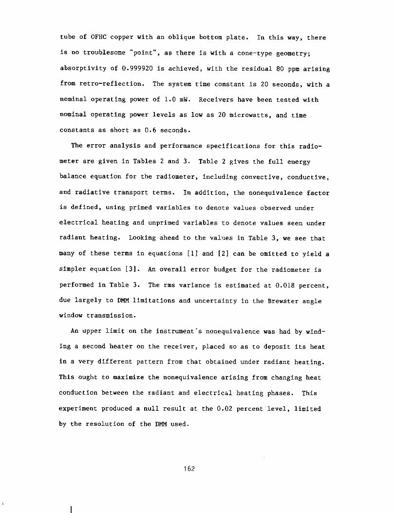
tube of OFHCcopper with an oblique bottom plate. In this way, there
is no troublesome "point", as there is with a cone-type geometry;
absorptivity of 0.999920 is achieved, with the residual 80 ppmarising
from retro-reflection. The system time constant is 20 seconds, with a
nominal operating power of 1.0 mW. Receivers have been tested with
nominal operating power levels as low as 20 microwatts, and time
constants as short as 0.6 seconds.
The error analysis and performance specifications for this radio-
meter are given in Tables 2 and 3. Table 2 gives the full energy
balance equation for the radiometer, including convective, conductive,
and radiative transport terms. In addition, the nonequivalence factor
is defined, using primed variables to denote values observed under
electrical heating and unprimed variables to denote values seen under
radiant heating. Looking ahead to the values in Table 3, we see that
manyof these terms in equations [i] and [2] can be omitted to yield a
simpler equation [3]. An overall error budget for the radiometer is
performed in Table 3. The rms variance is estimated at 0.018 percent,
due largely to DMMlimitations and uncertainty in the Brewster angle
window transmission.
An upper limit on the instrument's nonequivalence was had by wind-
ing a second heater on the receiver, placed so as to deposit its heat
in a very different pattern from that obtained under radiant heating.
This ought to maximize the nonequivalence arising from changing heat
conduction between the radiant and electrical heating phases. This
experiment produced a null result at the 0.02 percent level, limited
by the resolution of the DMMused.
162

Section 5: Calibrations usin$ the complete system
We have calibrated several silicon photodiodes against the radio-
meter using stabilized He-Ne and Argon ion laser sources. Calibra-
tions against the radiometer can be performed at any wavelength
between 260 nm and 2.0 microns, limited by the transmission of the
fused silica used for the Brewster angle window. Power levels from
0.1 mW to 2 mW may be made directly, with extensions beyond this range
by use of calibrated beamsplitters and attenuators.
The procedure was outlined earlier, and it consists of shining a
stabilized laser source onto the device to be calibrated, mounted on a
detector wheel. The detector response is noted, and then the detector
wheel is rotated to let light pass through to the radiometer. During
this phase, a dark reading is taken on the device being calibrated.
This is the radiant phase of a radiometer measurement. Once the re-
ceiver equilibrates, the temperature is noted, and the detector wheel
is rotated back. Once again the laser beam lands on the detector
being calibrated. Electrical heating is applied to the receiver cone
until the receiver cone temperature matches the earlier reading. The
cone heater power is noted, as it should exactly equal the radiant
flux.
Data from several calibrations of a single Si diode are presented
in Figure 10 and 11. Figure i0 shows the radiometer response to a
stabilized He-Ne laser beam, measured several times. If the beam were
absolutely stable, this only variations would be those due to the
radiometer readout noise. In fact, the rms variation of this data is
0.018 percent, which is nearly identical to the figure derived from
the formal error budget (0.019 percent). This implies that our formal
163

error budget overestimates the actual error, as there is a 0.01 per-
cent contribution from variation from variations in the beampower,
which predicts a total error of 0.020 percent.
Each point represents approximately 200 seconds of integration by
the radiometer. Note that for an instrument with a 20 second time
constant, this is i0 _, which may lead the reader to conclude that we
are waiting for the sytem to come to thermal equilibrium. Actually,
we use servo techniques to achieve an effective time constant of 1
second, so 0.01 percent measurementscan be madein i0 seconds. We
use a longer dwell time to reduce thermometry noise, which must be
reduced to a few microkelvin.
Figure 11 shows the response of a windowless Hammamatsumodel 1336
diode to the samestabilized beam. If the stabilized beamwere per-
fect, the only variations would be those due to the detector non-
uniformity and noise. The nonuniformity term occurs because the beam
did not always land on the sameportion on the detector. Detector
noise is vanishing for these devices, so the rms variation of 0.032
percent in the data implies that spatial nonuniformity in the diode
responsivity is the dominant source of the variations.
To complete the calibration, one simply divides the device response
by the beampower. Before presenting this data, we note that there is
an independent calibration we have performed which functions as a
check on the radiometric calibration. Specifically, we have performed
the method of diode self-calibration, developed by Zalewski and
Geist 9-11. This method involves measuring a series of correction
factors based on a model of the internal device physics of silicon
photodiodes; in this way, one can determine the absolute responsivity
164

of a diode detector.
This self-calibration is observed to be destructive to somede-
vices 12, so we performed it after the radiometer calibration is
complete13. The Zalewski and Geist self-calibration value is pre-
sented along with the radiometer calibration values, in Figure 12.
Again, each radiometer value corresponds to a single radiant/elec-
trical cycle of the radiometer, and a single diode reading. The
variance between the radiometer values is 0.028 percent, and the mean
of the radiometer values agrees with the self-calibration value to
within 0.01 percent.
It is interesting to note that the variance between successive
responsivity values is lower than the variance between diode readings,
which is 0.032 percent. This implies that there is somecorrelation
between the variations in the diode readings and variations in the
radiometer readings, as variations in the ratio are lower than in one
of the terms. The obvious meaning of this is that both the diode and
the radiometer are detecting drift in the stabilized laser beam, at
roughly the 0.01 percent level. Since detecting varying light levels
is the primary function of detectors, both diodes and radiometers,
this is hardly a shocking result.
Section 6: Summary
Results are summarized in Table 4. We have demonstrated stabilized
laser sources with intensity variations of less than 0.010 percent
over an hour. We have demonstrated a helium-cooled ESR absolute
radiometer with a standard error of 0.018 percent, and used it to
calibrate diode photometric detectors. An independent calibration of
165

a silicon diode was madeusing a technique based on the internal
device physics, and agreement was found to within 0.010 percent.
Capability was described for calibrating sources over the spectral
range 280 nm- 1.6 microns, and over the power range 0.1 mW- 2 mW.
This capability is felt to be of most importance for devices which
need absolute calibration to maintain stability over a long time, and
which lack a self-calibration.
Acknowledsements
This work was supported in part by N.B.S. contract #43NANB613437.
166

References
i)
2)
3)
4)
5)
6)
7)
8)
9)
I0)
11)
12)
13)
P. Foukal and P. Miller, Final Report on NOAA contract
NASORAC00204, 1982.
P. Foukal and P. Miller, SPIE Proceedings, 416, 197, 1983.
P. Foukal, C. Hoyt, and P. Miller, Advances in Absolute Radio-
metry, Proceedinss, 1985.
N. Fox, Advances in Absolute Radiometry, Proceedinss, 1985.
J. Geist, M.A. Lind, A.R. Schaefer, and E.F. Zalewski, NBS Tech-
nical Note 954, 1977.
H. Jacobowitz, H.V. Soule, H.L. Kyle, F.B. House, and Nimbus-7
ERB Experiment Team, J. Geophys. Res., 89, 5021-5028, 1984.
J.R. Mahar, Interim Report to NASA on Contract NASA-I-18106, 1987.
R.C. Willson, Applied Optics, 18, 179-188, 1979.
E.F. Zalewski and J. Geist, Applied Optics, 19, 1214-1216, 1980.
A.L. Schaefer, E.F. Zalewski, and J. Geist, Applied Optics, 22,
1232-1236, 1983.
J. Geist, E.F. Zalewski, and A.R. Schaefer, Applied Optics, 19,
3795-3799, 1980.
J. Verdebout, Applied Optics, 23, 4339, 1984.
As an aside, we do not find any degradation when Hammamatsu diodes
are calibrated; they require much lower voltages for the front
oxide loss measurement than do the E.G.& G. devices which have been
reported to exhibit degradation.
167

Author Address List
Miller, Peter J.
Cambridge Research and
Instrumentation, Inc.
21 Erie Street
Cambridge, MA 02139.
168

Table I. Presently available calibration wavelensths.
Wavelensth Laser Source Stability (est.)
325.0 nm He-Cd laser 0.04 %
351.1 nm Ar ion laser 0.04 %
363.8 nm Ar ion laser 0.04 %
442.5 nm He-Cd laser 0.028 %
457.9 nm Ar ion laser 0.028 %
488.0 nm Ar ion laser 0.028 %
514.5 nm Ar ion laser 0.028 %
528.7 nm Ar ion laser 0.028 %
532.0 nm Nd:YAG (doubled) 0.028 %
632.9 nm He-Ne laser 0.028 %
838.0 nm GaAIAs diode laser 0.028 %
1064 nm Nd:YAG laser 0.028 %
1153 nm IR He-Ne laser 0.06 %
1318 nm Nd:YAG laser 0.06 %
1523 nm IR He-Ne laser 0.06 %
169

Table 2. Radiometer Error Analysis
The radiometer equations are:
(TF 0 + Is a ) + Fbb s + Fra d + F+ cony = Fbbr + Fcond + F cony" [1]
F'bb r + F'cond + F-cond = Ehl h. [2]
where:
T l
F0 =
Is
a
Fbb s =
Fra d =
F+conv =
F
bbr =
Fcond =
F- =cony
cone absorptivity
Brewster angle window transmission
radiant flux
primary scatterer surface intensity
scattering solid angle
black body radiation from shields to receiver
black body radiation from window onto receiver
convective heat transport from cryostat to receiver
black body radiation from receiver to surroundings
conductive heat flow from receiver to heat sink
convective heat transport form receiver to cryostat
Unprlmed variables denote values observed during radiative heating.
Primed variables denote values observed when during electrical heating.
When F0 is in the mW range, an excellent approximation to Eq's 1 and 2 is
(TF 0 + Is a ) + Fra d + F+ =cony Fcond = Ehl h [3]
170

Table 3. Radiometer Error Terms
Term Magnitude Std. Error Percent Error
(0.4 mW signal)
0.99992 I0 ppm 0.001
T 0.99970 0.00008 0.008
Is 0.002 F0 0.001F 0 0.00008
a 0.0025 0.0008 Sr
Fbb s 0.I uW i00 pW 0.000025
Fra d 3.0 uW 30 nW 0.0075
F+conv 5 uW 20 nW 0.005
Ih 1.0 mA 0.01 uA 0.01
Eh 0.4 V 40 uV 0.01
Solving for the probable system error using Equation [3], we obtain:
F0 = 0.0186 %
171

Table 4. Capabilities of Laser/Cryogenic Radiometer Calibration
* Absolute calibration - permits long-term studies free of drift.
* Non-contact calibration - nondestructive of device being measured.
* Independant of device physics. Allows calibration of
devices which cannot be easily modelled or compensated.
* Device is calibrated outside of radiometer - no size or
environmental restrictions are placed on detector.
* Wide spectral range. Present system covers 280 nm- 1.6 microns,
but 244 nm- 10.6 microns is possible.
* Laser sources with excellent beam profile and low diffraction,
simplifies calibrations, compared to lamp or blackbody sources.
172

Laser Stabilizer
Slel)lllzed Source
IBM XT w/GPIB
Date ColleCtion Syclem
Dofleclor
Mirror
Deteclor
_'-'1 Wheel
Devices [_TO Be
Calibrated
(GPIB)
Brewster
Window
Cryogenic
Radiometer
Relerence Detector
Figure i. The detector absolute calibration system. Light from the stabilized
laser is presented to the cryogenic reference detector or to the detector
being calibrated.
Unstable
Laser
Source
Variable Attenuator
Input Pockels Exit
PoI. Cell Pol,
J Serve Amp _re_
and
H/V Amp
Control Electronics
Power Sensor
Beamsplitter
Stabilized
Laser
Output
Figure 2. Laser stabilizer block diagram. Light from an unstabilized laser
source is passed through an electrically variable attenuator. The setting of
the attenuator is servo-controlled so as to keep a fixed power level at the
output.
173

o
E_o
Unstabilized He-Ne beam
mma_
' o' ' _'_o 'I OOC' 2 DO ]_I) ¢ 5D(_C'
Seconds
BODO
Figure 3. Intensity variations in a He-Ne laser, without stabilization. The
readings are taken by a Hammamatsu 1336 windowless Si diode. This test spans
approximately i hr, and the laser is a linearly polarized Jodon laser operating
at 632.899 nm. The periodic variations in power level are probably due to
thermal expansion of the laser cavity, which shifts the cavity resonances
across the gain envelope of the atomic line which is emitting. The rms varia-
tion is 1.19%, and a bar representing a I milli-magnitude variation is drawn
for scale.
c
S_@bi}ized He-Ne beam
t
2
Jo 7.0{3 8.0E3
i J i i
90E3 I OOE3 t. 1E4 1 2 E4
Seconds
13E4
Figure 4. Intensity variations in a He-Ne laser, with stabilization. The
laser is identical to those of the previous Figure. These readings were taken
by a Hammamatsu 1336 windowless Si diode placed in the stabilized beam. For
this data, the rms variation is 0.010%.
174

o
i
¢o
E_
Stabilized He-Ne Beam
_. S.OE3 9.0E3 10.0E3 1,1[4 1.2E4 1.3E4
Seconds
1.4E4
Figure 5. Intensity variations in a He-Ne laser, with stabilization. This is
the data from Figure 4, redrawn on an enlarged scale. A bar representing a
i milli-magnitude variation is drawn for scale.
Unstable
Laser
Source
Variable Attenuator
Input Retardance Exit
Pol. Cell POL
Drive Amp
Conlrol Eleclronl¢s
Power Senior
Beamsplitter
(BK7 or KBr)
(InGaAs}
Stabilized
Laser
Oulput
Figure 6. Intensity variations in an 838 nm solid-state diode laser. This
test spans 1 hr, and the laser being stabilized is a D.O. Industries 25 mW
laser with integral collimated optics; the laser diode chip itself is a
Sharp device. The rms variation is 0.002%, and a bar representing 1 mmag
variation is shown for scale.
175

ooN
E_
Stabilized 858 nm beam
o_ 1.2E4 1.3E4 1 4E4 I _E4 I BE4 1.7E4
Seconds
BE4
Figure 7. Block diagram of the infrared laser stabilizer. Note that the design
closely corresponds to the stabilizer diagrammed in Figure 2, except for the
modulator and detector. A retardance cell replaces the Pockels cell, and the
monitor photodiode is made of InGaAs, not Si.
_ GRT
CRT.,, .......... // .......
/ $5 Heeter
Copper Near Wir_dings
Heat LpnW
Sm_
Rocho*ion
Figure 8. Diagram of the cryogenic radiometer receiver. Light incident on the
cone raises the temperature of the cone assembly above that of the heat sink it
is attached to. This temperature is noted, and then the light is shuttered and
electrical power deposited via the heater to achieve the same temperature. By
this substitution of electrical power for radiative power, an absolute reading
of incident flux is made.
176

Helium well fdllvenl
IN 2 well fill/venl
High vacuum port
Room letup wall
LN z shell
Helium well (3l)
Receiver
Radiation Shield
LN z cooled shield
Room _emp.
Mechanicol
ohgnment
Figure 9. The cryogenic radiometer assembly. Light enters at the bottom,
through a Brewster angle window (omitted for clarity), and passes through the
LN 2 shield and He-cooled radiation shield on its way to the receiver cone.
Liquid helium in the central well cools the heat sink and receiver assembly
to 4.2 K or lower.
o
O
o
E8
d
Rodiometer Response
D 0 q
6.5 ttm_ag
_3
I I I i i
1 2 3 4 5 B
Test Number
Figure 10. Radiometer response to a stabilized He-Ne laser. Each point
represents one reading taken by a substitution of electrical power for the
radiative power of the beam, and includes approximately 100 seconds of inte-
gration of the radiometer signal. The rms variation is 0.018%, and a bar
representing a 0.5 mmag variation is drawn for scale.
I?'7

oo
Z
o
3
_oO _>_
O. r
o
oo
r I
Diode Response
o [3
O, 5 _'+ag
Q 0
i I i I I
2 3 4 5 @
Test Number
Figure Ii. Response of a Hammamatsu 1336 windowless Si diode to a stabilized
He-Ne laser beam. These readings were interleaved between successive readings
shown in Figure 10. The readings were separated by approximately 2 minutes
from the associated radiometer reading. The rms variation of this data is
0.032%, which exceeds the variation in the radiometer readings and in the
stabilized source intensity. The excess variation may reflect spatial inhomo-
geneities across the photodiode face, as the beam illuminated slightly differ-
ent portions of the diode face on successive readings.
O
8
d
_cE
o
d
+mo
Diode Responsivity
y = . ]58848
I
+ i i + i
2 ] 4 5 5
Test Number
Figure 12. The diode responsivities calculated from Figures 10 and 11. The
observed diode current is divided by the radiometer reading of beam power to
determine the diode responsivity. The dashed line represents the diode
responsivity calculated independently using the self calibration method of
Zalewski and Geist. The rms variation of responsivity values is 0.028%
(0.3 mmag), while the mean of the population agrees with the independentlydetermined value to within 0.010%.
178