-N1. DOC.

'3J')2i/.' 1./2Q3

NATIONAL ADVISORY COMMITI'EE

FOR AERONAUTICS

TECHNICAL NOTE 2239

THEORETICAL INVESTIGATION OF TRANSONIC SIMILARITY

FOR BODIES OF REVOLUTION

By W. Pen and Milton M. Klein

Lewis Flight Propulsion Laboratory Cleveland, Ohio

Washington December 1950

BUSINESS, SCIENCE & TECHNOLOGY DEP'L

DEC 18 1950

https://ntrs.nasa.gov/search.jsp?R=19930082881 2020-06-07T16:40:21+00:00Z

NATIONAL ADVISORY COMMITTEE FOR AERONAUTICS

TECBNICAL NOTE. 2239

TEEORETIC.AL INVESTIGATION OF TRANSONIC SIMILARITY

FOR BODIES OF REVOLUTION

By W. Pen and. Milton M. Klein

SUMMARY

A solution for the compressible potential flow past slender bodies of revolution has been derived by an iteration procedure similar to that of the Rayleigh-Janzen and Prandtl-Ackeret methods. The solution has been analyzed with respect to traneonic similarity. The results obtained are in approximate a'eement with those of von Karmn in the region of the flow field not too close to the body. In the neighbor-hood of the body, a different similarity law is obtained. This new similarity law holds for variations in thickness ra.tio and Mach number, but not for variations in specific-heat ratio. In addition, this law appears to be limited, in applicability to extremely lender bodies of revolution probably outside the range of practical interest. The dif-ferences between the results of. the present investigation and those of von Krmn are interpreted in terms of the manner in which the. boundary condition on the body is satisfied and of the nature of the singularity. of the solution near the axis.

INTRODUCTION

Tran_sonic similarity rules for thin airfoils and. slender bodies of revolution have been derived by von Krnin (reference 1). These rules for the case of two-dimensional flow are verified In reference 2 by an iteration procedure similar to that of the Rayleigh-Janzen method (ref-erence 3) and the Prandtl-Ackeret method (reference 4).

The analogous investigation for bodies . of revolution was made at the NACA Lewis laboratory and is presented herein. A solution f or the compressible potential flow past a slender body of revolution is obtained by the sane iteration and transonic limiting procedure used In reference 2. As in reference 2, in each step of the iteration procedure the boundary conditions were satisfied on the body.

The solution obtained yielded transonic similarity rules that are,. in part, different from those of reference 1. The differences appear to result from the. method of satisfying the boundary condition on the body and from the nature of the singularity of the solution near the axis.

2 NACA TN 2239

As in the two-dimensional investigation, the influence of stag-nation points has not been considered herein.

ANALYSIS

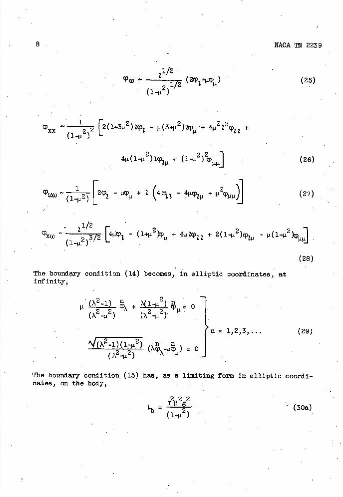
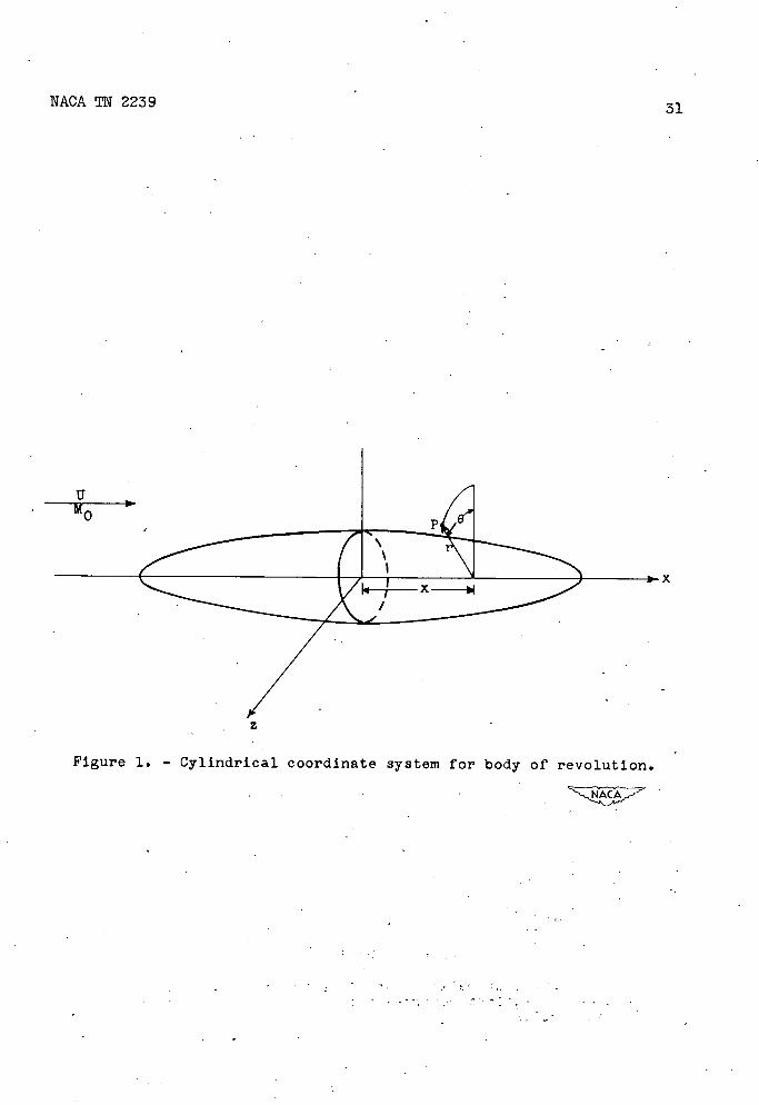
General formulation. - The partial differential equation for a compressible, axially symmetric, isentropic and irrotational flow with free-stream velocity U in cylindrical coordinates x,r,e (fig. 1) is

[a2 - (U+u)2]cp + ( a2 -v2 ) prr - 2(U+u)rp2 Pr

+a —=0 (1) xi'

in which the following notation has been used:

a local speed of sound

U+u resultant velocity in x-direction

v resultant velocity in r-direction

' perturbation velocity potential defined by u = Cp, v = (Subscripts denote differentiation with respec,t to variable noted.) (All symbols used herein are defined in the appendix.) The local speed of sound a is related to the free-stream speed of sound a0 , the ratio of specific heats y, and the local velocity by the Brnou1li equation

a2 = a02 Z (2Uu + U2 + v2 ) (2)

In accordance with the Prandtl-Ackert type of procedure, equation (1) will be written in a form In which the linear terms appear on the left side of the equation and the nonlinear terms on the right side. A solution will then be sought in the range of free-stream Mach number close to land thickness ratio close to 0 on the assumptionthat the flow pattern obtained. by inclusion of the nonlinear terms will differ • by only a small amount from that obtained with only the linear terms. This assumption will then be made plausible by the resulting form of the

solution. The coefficient of cp in equation (1) . is therefore expressed, with the aid of equation (2), Inthe form

a2 - (U^u) 2 = 2a2 - 2fr [(u)2] 7 (3)

NACA TN 2239

3

where

M0 free-stream Mach number, U/a0

= l-MO2 (4a)

"N = MO2 (i + z::i MO2) 0

(4b)

For convenience, the free-stream velocity is taken as the unit velocity so that u/U, v/U, and. cp/U maybe written as u, v, and. cp, respeQtively. The differential equation (i) can now be expressed in the form

12+)[l Z!MO2(2q,14q2^cc,2)]

(3

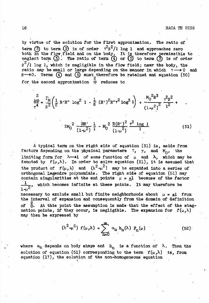
= [rM(2,X+2) + Zji M0 cP] cp + Mo2 r2 i, + 2MO2 ( l4 x)cPra. (5)

The boundary conditions of the problem are: (1) The perturbation velocities vanish at infinity, and (2) the flow follows the contour of the body. Thus, at infinity,

cp = r = 0 (6)

arid on the body,

rb Tg(x) (7a)

= T(i4) g(x) (7b)

where 0

¶ lateral distance ratio of body

g(x) function characterizing shape of body and. of order of magnitude 1

4

NACA TN 2239

All len€ths are expressed in terms of the chord of the body as 1.

In order to obtain the Laplacia.n of on the left side of equation (5), the affine transformation

(8)

is introduced. The differential equation (5) becomes

= zj:L 2(2 222) +

[ (pq2) + %-4

cP+

-

2MO2(l4p)%,cp, (9)

where the Laplacian of cp in cylindrical coordinates is

(10)

The boundary conditions. (7a) and (7b) become,

at infinity,

(ii)

on the body,.

W.b=13 g(x) (12a)

cp_ :. g(x) cp = g(x) (12b)

The formulation of the problem so far is exact. A solution is now sought that is applicable in the range T and. 13 close to zero (r- 0, -0). This solution is referred to hereinafter as "the small-perturbation

transonic limiting solution." In the range of .T and f3 under considera-tion (T'-O, -0), the perturbation velocities will be assumed small

NACA TN 2239

5

compared. with free-stream velocity or Iu((< 1, IvJ<< 1. Thus, as is usual in this type of procedure, the right sid.e of equation (9) is considered. to produce a small perturbation from the linear case and. a solution of the system of equatIons (9), (ii), and (12) will be sought in the form

12 3(13)

In which each term is of a lesser order.of magnitude than the preceding 12

one. The following boundary conditions on q, q) , . . . will accord-irigly be taken as the equivalent of the boundary conditions (11) and. (12):

=0; n = 1,2,3, . (14)

= t3T g(x) (15a)

1 .g(x)cp1 = g(x) (15b)

At Infinity,

U cpx

On the body,

1

fl T TI - rii (15c)

In order to obtain a solution of the system of equations (9), (13), (14), and. (15), equation (13) is Inserted Into the differential equatIon (9) and. a typical Laplaclan term on the left, such as 4, is equated to the sum of those terms on the right that contain the super-script n-1 and. that may also contain any of the superscripts n-2,

n-3, . . . 1. The right side of the differential. equation for con-

sists of a sum of terms of which, for a range of M near 1 and. T

near zero, sczne will be of highest order of magnituae. The solution corresponding to these terms constitutes the small-perturbation tram-sonic limiting solution for

Transformation to prolate-elliptic coordinates. - For the problem - of the flow past an Isolated body of revolution, It is convenient In satisfying the boundary conditions to use a system of prolate-elliptic

6 'NACA.TN 2239

coordinates (reference 5). The transformation from cylindrical coordinates x, to elliptic coordinates .t,X is. given by

x =p)

(168)

Co = -(X2_l)(1_12) (16b)

The surfaces = constant, .x = constant are confocal ellipsoids and hyperboloid.s of 1vo sheets, respectively, the cxmion foci being at x 1, (0=0. The values of may range from 1 to infinity, whereas i varies between -1 and +1.

The Laplaclan of cp is, in elliptic coordinates,

[2l) (17)

Transformations from derivatives with respect to x and (0 to derivatives with respect to t and. ?' will be needed for subseg.uent analysis. om the transformation equation (16), these relations are

_______ 7(l_2) cp (18) = (\22) q7^ (X22)

w=2l)(12)

(19).

= (2l)(l2) [ (+3) 232] 2(2l)2 ^

(?-.)

2(2)(2_1)q,+ (20)

NACA TN 2239 7

________ 2 2 2

(22)3x +

(2l)(l2)

+- (21)

(?-)

x=( 2 l)( 1 2 ) r 2(2) + 2(l32)1

(22)2( - 2 2

+ 2 ( l3 2 +

[(22)

2 2 2

(21) (22x - (l2)p (22)

The variable X has the lixnitin€ value 1 on a body of revolution as the thickness ratio T of the body approaches zero. It will there-fore be convenient to have the limiting forms, for \ -'1, of equations (18) to (22). DefinIng a new variab1e.. Z by

1 = (23)

and. denoting by - the limiting form for ?-. 1, equatIons (18) to (22) take on the limiting forms

l-j.+ cpM (24)

8 NACA TN 2239

l/2 -

1/2 (2p) (25)

(l-t

xx (i_) [2(l^32)2 - (3 2 ) 422 +

4ii(l—i2)2cp1 + (l_L 2 ) 2cp 4t1 (26)

l_2) [2i4 - +

(27)

• 1/2

(U(l_)3/2

[4iq,1 - + 4tlq 1 + 2(l-2)cp1 -

• (28)

The boundary condition (14) becomes, in elliptic coordinates, at infinity,

p2i) 2 2 • 2 2. I

= 1,2,3, (29)

j (2_2) (?cptcp) = 0

The boundary condition (15) has, as a limiting form in elliptic coordi-nates, on the body,

22(30a)

(l- )

NACA TN 2239

9

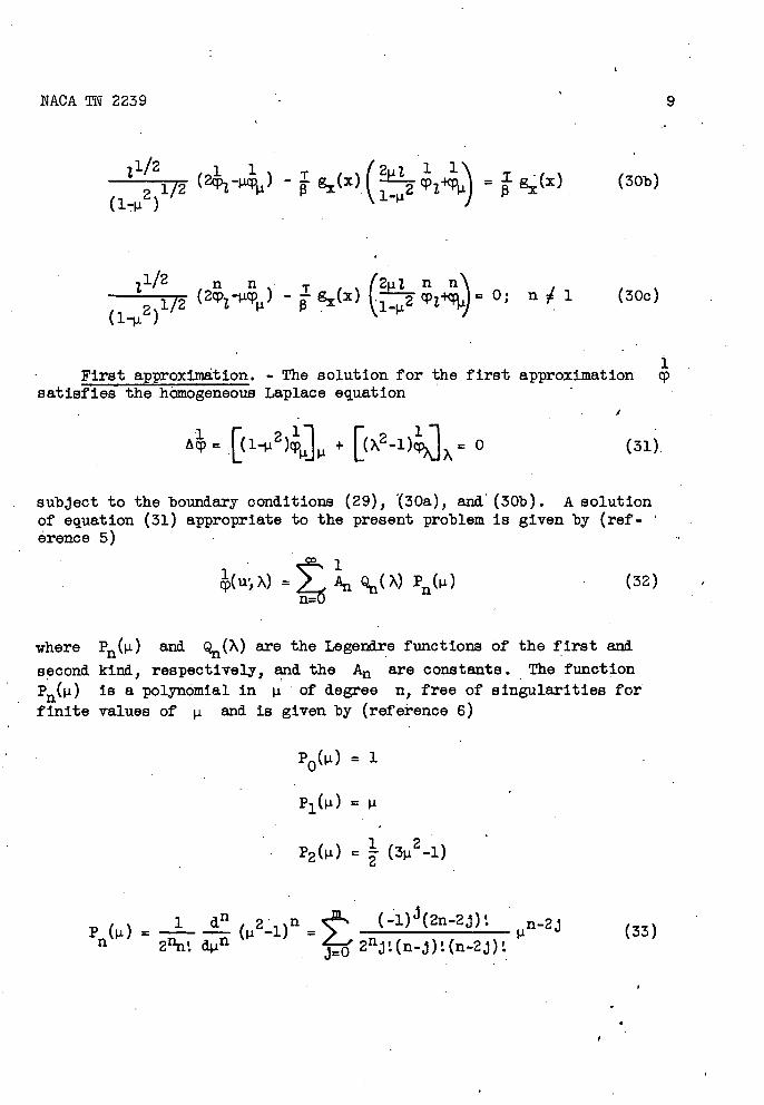
2 1/2 ____

2V2(X)(2 l l\

(l- )i-L

= - g(x) (30b)

21/2 T I2jtl n

2)h/2 (2q2-tcp) - - g(x) i2

0; n 1 (30c)

1 First approximation. - The solution for the first approximation q

satisfies the homogeneous Laplace equationI

= [(1_ 2)j ,, + [( x2_1Tj = 0 (31).

subject to the boundary conditions (29), (30a), and (30b). A solution of equation (31) appropriate to the present problem is given by (ref-erence 5)

(u',?) = A %(?) P() (32)

where P(i.i) and are the Legendre functions of the first and

second kind, respectively, and the A are constants. The function

P(i i ) is a polynomial in t of degree n, free of singularities for finite values of .i and is given by (reference 6)

P0 (.i) = 1

= P.

P2 (P.) =(32k)

1 drl ________________

= 2(2l)fl = (1)i(22j)

n-2j P. (33)

j=0 2njt. (n-i)'. (n_2j)'.

10 NACA TN 2239

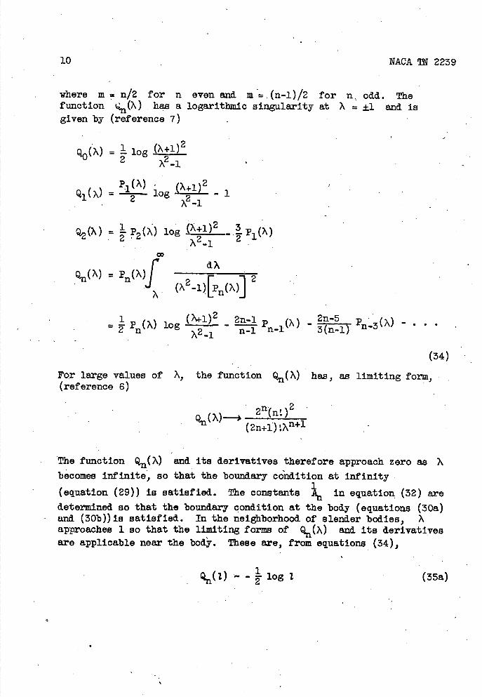
where m = n/2 for n even and. m (n-1)/2 for n odd. The function X) has a logaritbmi.c sin€ula.rity at X = ±1 and. is given by (reference 7)

= log

= log +i)2 -

Q2(?) = 2log (X+i)2 -

X-i

dX

=(2\21)[P(\)] 2

P(?) (2i)2 2n-1 p (7) - 2n-5 Pn..3(X) - • log --

n-i n-i 3(n-l)

(34)

For large values of \, the function Q( has, as limiting form, (reference 6)

2n ,2 Q(X)—* 1.j

(2n^l)X"1

The function Q(\) and its derivatives therefore approach zero as l

becomes infinite, so that the boundary condition at infinity

(equation (29)) is satisfied. The constants in equation (32) are

determined so that the boundary condition at the body (equations (30a) and. (30b))is satisfied. In the neighborhood. of slender bodies, ) approaches 1 so that the limiting forms of Q(7) and its derivatives are applicable near the body. These are, from equations (34),

- - log 2 (35a)

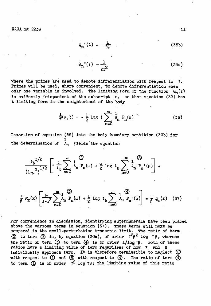
NACA TN 2239 11

- - (35b)

Q"(l) (35c) 21

where the primes are used to denote differentiation with respect to 1. Primes will be used, where convenient, to denote differentiation when only one variable is involved. The limiting form of the function (l) is evidently independent of the subscript n, so that equation (32) has a Limiting form in the neighborhood of the body

1 1 c'l = - log 2

A Pn(1) n=O

Insertion of equation (36) into the body boundary condition (30b) for 1

the determination of A yieldsthe equation

I- cØ lbl/'2

- 1n + - log 2b A1 P' (ii +

(l_2)hI2 L n=O n=O

p.®

g(x) [l2 P() + log 2b fl Pn '( j = I (') (37)

nO n=O

For convenience in discuss ion, identifying supernumerals have been placed above the various terms in equation (37). These terms will next be compared in the small-perturbation transonic limit. The ratio of term () to term (I) is, by equation (30a), of order 722 log T, whereas the ratio of term ( to term ® is of order l/logT. Both of these ratios have a limiting value of zero regardless of how T and. individually approach zero. It is therefore permissible to neglect © with respect to © and. © with respect to ®. The ratio of term ® to term © is of order T2 log i; the limiting value of this ratio

(36)

- Kgg pt()-7

2

fl: ii=0

K= T 2 log 113

where

(38)

(39)

12

NACA TN 2239

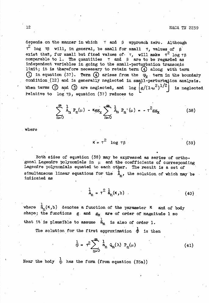
depends. on the manner In which T and. J3 approach zero. Although

log T will, In general, be small for small T, values of 13 exist that, for small but fixed values of. T, will make ¶2 log T13 comparable to 1. The quantities ¶ and. 13 are to be regarded. as independent variables in going to the small-perturbation transonic limit; it is therefore necessary to retain term ® along with term () In equation (37). Term arises from the . term in the boundary condition (12) and. is generally neglected. In small-perturba4ion analysis.

When tsrms ® and (j) are neglected, and log [g/(l_,12)JJ2J is neglected

±'elative to log TJ3, eq .uation (37) reduces to

Both sides of equation (38) may be expressed as series of ortho-gonal Legend.re polynomials in .t and the coefficients o± corresponding Legendre polynomials equated to each other. The zesult is a set of

simultaneous linear equations for the A, the solution of which maybe indicated as

= ¶2c,b) - (40)

where (K,b) denotes a function of the parameter and of body shape; the functions g. and gx are of order of rna€nitude 1 so

that it is plausible to assume Is also of order 1.

The solution for the first approximation Is then

= a () P(i.) (41) n=O

Near the body has the form (from equation (35a))

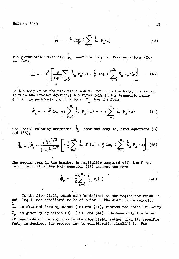
NACA TN 2239

13

1 2 cp--T 1O€>2k1p() (42)

n=O

The perturbation velocity near the body is, from equations (24) and. (42),

- - T + log k1 P'( (43)

On the body or in the flow field not too far from the body, the second term in the bracket dominates 'the first term in the transonic range - 0. In particular, on the body cp haè the form

1 2 - T log T >2k1 P'() = - > i• P'() (44)

n=O nO

• The radial velocity component near the body is, from equations (8) and. (25),

T2l1/ r

>2 P) + log 1 a pt.( (45) =L n=O n=o /

The second term in the bracket is negligible compared with the first term, so that on the body equation (45) assumes the form

1

- - L a (46)

Inthe flow field, which will be defined as the region for which 1 and log 2 are considered to be of order 1, the dietrubance velocity

is obtained from equations (18) and. (41), whereas the radial velocity

is given by equations (8), (19), and (41). Because only the order

of magnitude of the solution in the flow field, rather than its specific form, is desired, the process may be considerably simplified. The

14

NACA Th 2239

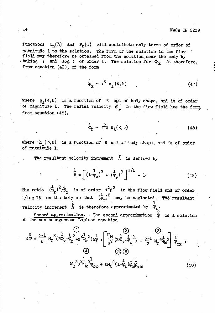
functions Q() and P(i.i) will contribute only terms of order of

magnitude 1 to the solution. The form of the solution in the flow field may therefore be obtained from the solution near the body by taking and. log 2 of order 1. The solution for Is therèf ore, from equation (43), of the form

1 2

- T 1 (K,b)

(47)

where g1 (K,b) is a function of I and. of body shape, and. is of order of magnitude 1. The radial velocity cp in the flow field has the forn

from equation (45),

- h(K,b)

(48)

where h( K,b) is a function of C and of body shape, and is of order of magnItude 1.

1 The resultant velocity increment A is defined by

1 1 2 1 2 1/2 A = [ (i.t) + r? I - 1 (49)

The ratio ( 1 )2/

Is of order ¶232 in the flow field and. of order

1/log Tf3 on the body so that (cpr) may be neglected. Thé resultant 1 1

velocity Increment A Is therefore approximated. by q,.

Second approximation. - The second approximation cp Is a solution of the non-homogeneous Laplace equation

© H®

2 y-1 2 1 1 2 2 1 2 i 1 2Mo4%21 1

2 M0 (2 x + + xx

1 11

+ (50)

NACA TN 2239

15

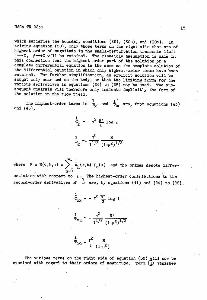
which satisfies the boundary conditions (29), (30a), and. (30c). In solving equation (50), only those terms on the right side that are of highest order of magnitude in the small-perturbation transonic limit T—+ 0, 3—)0 will be retained. The plausible assumption is mad.e in this connection that the highest-order part of the solution of a complete differential equation Is the same as the complete solution of the differential equation in which only highest-order terms have been retained. For further simplification, an explicit solution will be sought only near and on the body, so that the limiting forms for the various derivatives In equations (24) to (28) may be used. The sub-sequent analysis will therefore only indicate implicitly the form of the solution in the flow field.

The highest-order terms in and are, from equations (43) and (45),

1 ci, - - T2 !- log Z

1 T2 R ci:0)'--

1[2 (l.t2)]/2

where B = R( ,b,) =

k,b) (i) aM the primes denote differ-

entiation with respect to The highest-order contributions to the

second-order derivatives of ci, are, by equations (41) and (24) to (28),

1

xx 2.1ogi Ci, .-T

- z 1/2 (l-2)1/2

1 2B

T(12)

The various terms on the right side of equation (50) will now be examined with regard to their orders of magnitude. Term (J vanishes

16 NACA TN 2239

by virtue of the solution for the first approximation. The ratio of

term to term () is of order i2/z log 1 and. approaches zero both in the flow field and on the body. It is therefore rmissible to neglect term ® The ratio of term or to term is of order

log 1, which is negligible in the flow field; near the body,. the ratio may be small or large depending on the manner in which T-* 0 and.

—+0. Terms and () must therefore be retained, and equation (50)

for the second approximation reduces to

= - B 'R" log2 2 - (R' ) 2R"T2 log3 )

MO2R3 T22

T4 2 2 + ( 1_2)2 i2 +

2 RB' 1 2 R(R') 2 'r2 log i 2M0 (1 2) - M0 2 (51)

- (i-p)

A typical term on the right side of equation (51) is, aside from factors depending on the physical parameters T, y, and M0, the limiting form for —+1 of some function of .i and X, which may be denoted by f(p,?). In order to solve equation (51), it is assumed that

the product of f(t,X) and (?2I.L2) may be expanded into a series of orthogonal Legendxe polynomials. The right side of equation (51) may contain singLilarities at the end points = +1 because of the factor

1 , which becomes infinite at these points. It may therefore be 1 necessary to exclude small but finite neighborhoods about = ±. from the interval of expansion and consequently from the domain of definition

of . At this point the assumption is made 'that the effect of the stag-nation points, if they occur, is negligible. The expansion for f(,i,?) may then be expressed by

(22) f(1i,7) = cz.h() P(i) - (52)'

• where a. depends on body shape and h is a function of . Then the

solution of equation (51) corresponding to the term f(t,7') is, from equation (17), the solution of the non-homogeneous equation

NACA TN 2239

17

( 22 ) [(x2_i)cp] = rS Un hn(?) P(I.L) (53)

A. solution of equation (53) is now sought in the form

= cX q(X) P(pi) (54)

where q(?) Is a function of ? to bed.etermined.

- Inserting equation (54) in quation (53) and. noting that satisfies Legen&re's differential equation yields, when coefficients of

are equated. the non-homogeneous Legendre d.ifferential equation

[(? 2 _1) q, t (?)] n(n^1) q(X) = h() (55)

The solution of equation (55) is the sum of the complementary solution taken proportional to %(X) to satisfy the boundary condition at infinity an&the particular inteal r(X), which may be expressed in terms of two indefinite intea1s by

r(X) = Pfl(X[[21 P?(fhhh1 Pn(X)dXi (56)

The function ru satisfies the boundary conditions at infinity. The solution of equation (53) may therefore be written as

= T[ A Q(X) n()

+

r() P( (57)

The limiting form of equation (56) for —+1 or l—"O is

r(l) - J' ijh(i) d.l (58)

18

NACA TN 2239

The subscript n is omitted from r(l) inasmuch as h() is

independent of the subscript n in the limit l—,O. Equation (57) then becomes, for l-30,

[.

log Pi) + r(l) a (59)

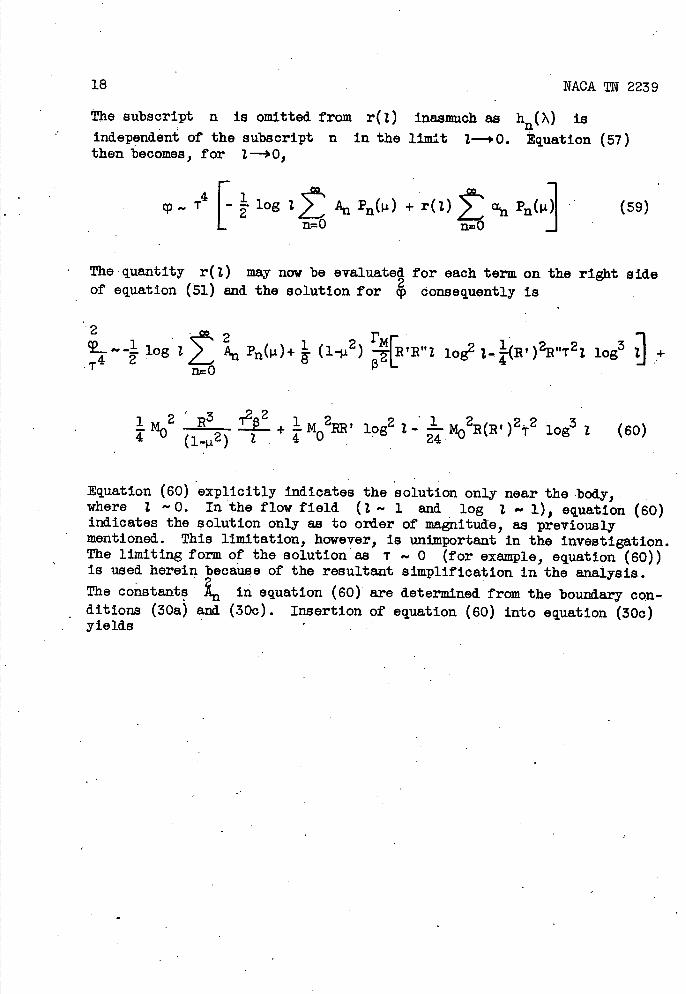
The quantity r(2) may now be evaluated for each term on the right side of equation (51) and. the solution for p consequently is

2 T_.._l log2 (l-ii2) [R'R"l 1og22_(Rt)2RhiT2z log3 ] + T4 n0

i 2 R3 122 + I M 2, log2 2- MO2R(R' ) 2T2 log3 2 (60) .M0 (1_i 2 ) 2 4 0

Equation (60) explicitly indicates the solution only near the body, where 2 -0. In the flow field (1 - 1 and. log 2 1), equation (so) indicates the solution only as to ord.er of magnitude, as previously

• mentioned. This limitation, however, is unimportant in the investigation. The limiting form of the solution as T - 0 (for example, equation (60)) is used. herein because of the resultant simplification in the analysis.

The constants in equation (Go) are determined from the boundary con-

ditions (30a) and (30c). Insertion of equation (60) into equation (30c) • yields

NACA TN 2239

19

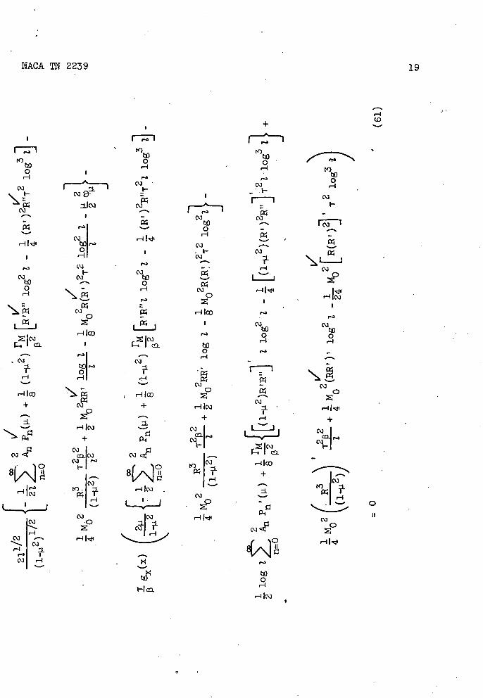
H + (0

F .- I

0 H - 0 H _

0 H 9-

I

I

-

r- 1 0 HN4 H

0 cJ—

—

H I I 0 H

—I

- Hl '-3 '-3

IZ I I 1 Hico 0 0

I (0- H H 0 r-3

v-31

(\)H -

-

0 a H cz _

Hjo 0-

0 + HI C3 a-- HI z + I H +

+c'i

'-3

I- 9-c ZIc3 ci - C'-)F \o

Hico i +

" 0- HI -H _

1:1 _____lilt -

0

0 Ic' ('Jo

•0

81,,.\JHNI

'-3

•

Hai0 H

HIC)

20

NACA TN 2239

-, 222 where 1 is to be evaluated at = The unchecked terms in

i_2 equation (61) become negligible compared with the checked terms in the small-perturbation transonic limit. Equation (61) therefore reduces to

- Kgg

= log T (2MQ2 t + [r 2RtRtt_ 2R(R t ) 2 g (pp)] -

K2 g2()2tt - j MO2 [RRt ) 2]I) (62)

Equation (62) may be solved for the coefficients. in the same manner

as was indicated for the coefficients A occurring in the first approximation c5. in equation (52), it may be necessary to exclude the region around. the end. points = l. The result thay be expressed as

2 2 = log T K,MO,rM,b)

where K,MQ,FM,b) denotes a function of th6 parameters K, M0, rM,.

and. the body shape and. is of the order of magnItude 1.

Although the term In B 3 cannot be neglected in equation (51), it. can be neglected in equation (60) and. in the boundary condition

(equation (61)). Near the body, the solution for given by

equation (60) therefore becomes, when the B 3 term is neglected.,

21

- - log T log 2 z.. an Pn + (l_2)._[RtRhhz log2 2 -(R' )2RttT2log3 i]+

n=0

1 2p(Rt)272 log3 2 (63) log2 2 -

NACA TN 2239

21

An explicit solution for the potential in the flow field cannot be obtained from equation (63) but, as previously mentioned, the order of magnitude of the solution in this region ma be inferred from equation (63) by taking 2 and log 2 of order 1. In the flow field,

the disturbance velocities and. thus have the form

72 (cK+cC) (64)

2. 7

where c= c ' .1

shape, and. c2 and c's and d's . are

= -T2t3(d1K+d2E) (65)

and. d1 are functions of K, M0, rM, and. body

d2 are functions, of only K and. body shape. The f order of magnitude 1.

In the nei&aborhood of the body (equation (30a)), the quantity 1 begins to contribute to the order of magnitude of the terms in equation (63). The disturbance velocities on the body are thus given by

K2 P'() + MO2 (RR')' - R(Rt)21'K (66)

CPr - P) - 2MoRRi + [MO2R(Rt )2 - rg2RtRt K +

. F Mg (R ) R"K (67)

2 Aside from the dependence of the constants a on K, the dominant

terms contributing to on the body (equation (66)), come from the

terms in the differential equation (50). The first 2 11

term of in the flow field. (equation (64)) results from the qcp1

term. The second term of equation (64) comes from the term in

in equation (50). The expressions for on the body and. in the

flow field (equation (67) and. (65), respectively) may be similarly ,analyzed.

22 NACA TN 2239

DISCUSSION

Traisonic similarity. - The results obtained, thus far in the first two approximations may be summarized as follows:

On the body,

- - [ + (s 0 ') ^ MO2 R(R')2 K2] (68)

- +[st 2 (p i )] + M 2 [R(R1 )2] K (69)

+ [MO2R(RI)2 - + rgRt)R13

- (70)

where

SnP(t)

In the flow field (i - 1, log 1 - 1),

-Cp - T 2 (b1 + b2 +b3 ) (71)

x T2 l +C2 K+C3E ) (72)

I

NACAITN 2239 23

where b2 , c2 , and d2 are functions of Pt, M0 , r 4, and body shape and the other b's, c's, and d's are functions of only Pt and body shape. The b's, c's, and d's are of order of magnitude 1. It appears plausible to assume that higher approximations would not alter the results obtained thus far concerning the dependence of the potential on the parameters Pt and C.

The solution given by equations (68) to (73) will next be considered from the viewpoint of transonic similarity; that is, the possible dependence of the solution on less than three combinations of the physical parameters T, Mtj, and. y in the small-perturbation tran-sonic limit T—)0, 3-30 will be investigated. In the limit T—+0, 13—+0, the solution for the body (equations (68) to (70)) becomes a function of the parameter Pc, the ratio of specific heats y, and the body shape. Hence, for constant y, a similarity rule exists on the body with respect to variations in T and j3 through the similarity parameter K. In the derivation of this result, it was necessary to neglect tentis of order 1 in comparison with log 1; that is, in compari-son with log T3 on the body. The quantity 1, however, must be extremely small before log Z begins to dominate terms of order 1. The foregoing similarity rule may therefore ' possibly be limited, to extremely slender bodies with thickness ratios not in the range of practical interest. If the body is not extremely slender, the potential in the neighborhood of the body depends not only on the parameter Pt but also on the thickness ratio T in a complicated manner. (See, for example, equations (41) and. (63).)

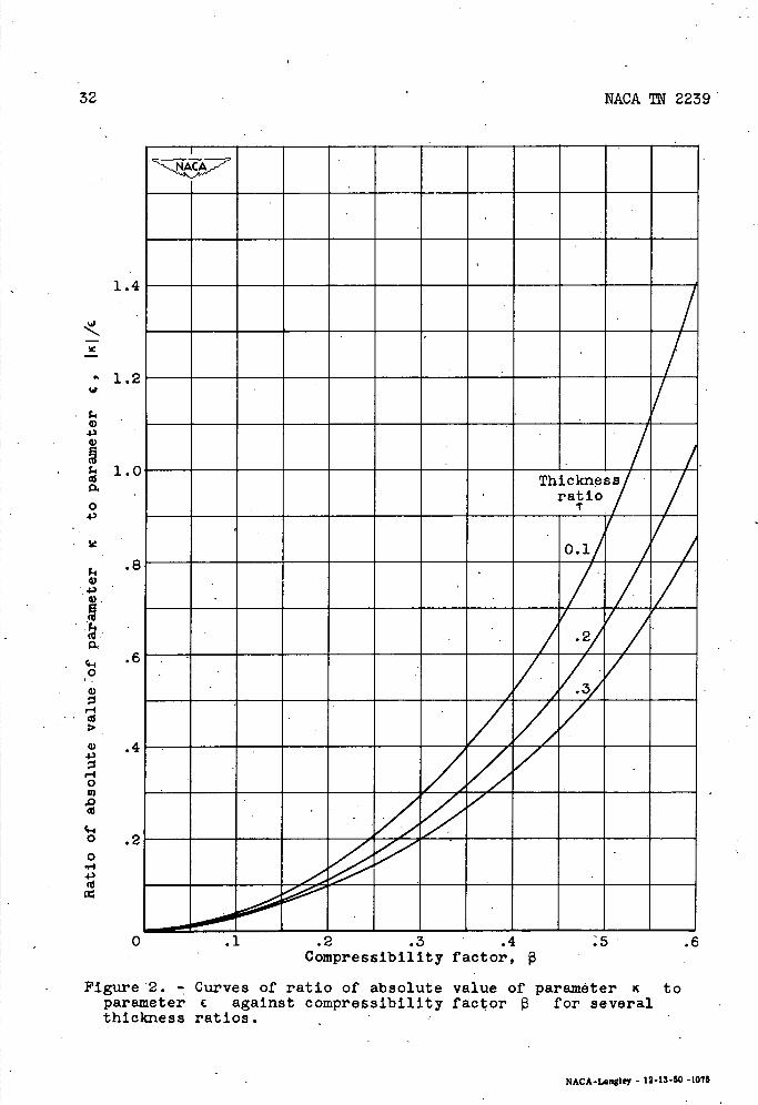
For the flow-field solution, (equations (71) to (73)), in the limit T-30, f3—+0, the coefficients b2 , 02, and d2 become functions of Pt, y, and body shape, whereas the other b's, c's, and d's remain functions of Pt and body shape. The flow-field solution thus becomes, for T—^0, 3-0, a function of three parameters Pt, c, and. ', so that apparently no simple similarity law exists in the flow field. The original physical parameters of the problem (T, M0, and y) have not been reduced in number, so that no apparent simplification of the dependence of the potential upon the physical parameters has been achieved. Figure 2, which presents curves of IKI /c against J3 for several values of the thickness ratio T, shows, however, that the parameter C is much larger than the parameter Pt for small values of 3. It then appears desirable to consider those flow-field solutions in which c Is of order of magnitude 1 and. K is negligible compared with C.

The essential modifications in the analysis previously given are that the term in Cp in the body boundary condition (7b) may now be neglected in view of equation (38) and that only the terms in

24

NACA TN 2239

cpq need be considered on the right side of the differ-

ential equation (9). The term in is the dominant term in the

flow field, whereas the cpcp and. terms are dominant in the

neighborhood of the body. It is therefore necessary to retain the

terms and for the body boundary condition in order to

obtain the constants A of the complementary solution.

By carrying through the analysis directly or by inspection of the solution equations (71) to (73), the potential in the flow field may be expressed in terms of the single paranieter c. Because of the siinp1ifi-cations resulting from the condition K<<c, this analysis for the solution in the flow field. has been carried through the first three approximations. In the third approximation, as well as in the second approximation (equation(63)), the complementary solution becomes negligible comoared with the particular solution corresponding to the cpcp term in the flow field. Thus the results for the flow-field region to three approximations may be expressed as

F = f1c + f2 €2 + f3c 3 (74)

where

F=--cp (75)

and f1, f2 , and f3 are functions only of body shape and are of

order of magnitude 1.

In establishing equation (74), it was unnecessary to make the strong assumption log l>>l but rather the much weaker ones, r 2<<l, 32<<l and. log T3 1. It Is therefore probable that the similarity law for the flow field given by equation (74) holds for a wider range of thickness ratios than the similarity law for the body (equation (68)). The existence of different similarity laws for the flow field and for the body would, indicate a transition region where a more complicated relation. obtains.

Comparison with reference 1. - The results obtained. In this investi-gation are somewhat different from those of reference 1, where a single similarity parameter equivalent to the parameter c Is derived for both the flow field. and the body. These differences may perhaps be understood as follows:

NACA TN 2239 25

In reference 1, the boundary condition at the body is written in a form essentially equivalent to

'Wr = T2gg for r—,O

or

(OFw = gg - for w—*O (76)

and. nonlinear terms in the differential eq .uation for the potential other than the term are neglected. When only the term on the right side is retained and the transformed potential F is used, equation (9) becomes

= 2FF (77)

If it is assumed that the boundary condition (76) may be evaluated on the axis = 0 rather than on the body 0b = T3 g(x), then the only

parameter entering the differential equation (77) aM the boundary condition (76) Is c. The potential F(x,W) should therefore be expressible in terms of the single parameter C. On this basis, the transonic siMlarity rules in terms of the parameter € are :obtained-iii reference 1..

The present analysis differs from that of reference 1 in three respects. First, the boundary condition (26a), or, more 'generally, the boundary condition

= +fl gflg -( 78)

is, in the present analysis, satisfied on the body, as

rb = Tg(x) (79)

rather than near the axis, as

r—O (80)

The use of equations (78) and (79) will evidently yield the same results for any value of the exponent n. Equation (80), however, is equivalent

26

NACA TN 2239

to equatlon (79) only if n = 1, and. then only in the first approxi-mation; for in the first approximation (equation (41)), - log r, so that rq, has a finite nonzero limit as r—*O.. Hence, reference 1

is correct insofar as the first approximation obtained herein is concerned.

In the second approximation (equation (63)), however, the dominant

2 2 term is of order log r so that rq) becomes infinite for r---, 0. This result, however, does not invalidate the procedtre as regards the flow field because the boundary condition (76) is needed only to obtain the complementary solution in equation (63). As previously noted, the complementary solution is negligible with respect to the particular solution corresponding to the FxF term in the flow field, at least to the first three. .approximatfons.

A second. difference between the present analysis and that of reference 1 stems from the logarithmic-type singularity that the potential cç(x,r) exhibits as r—O. This singularity affects not only th numerical value of the potential cp(x,r) and. the.velocity at the body rb =Tg(x), but also its order of magnitude. Hence, even after use of equation (79) in satisfying the boundary condition, a further use of equation (79) xnust be made in the solution to determine the parameters on which the velocity at the body depends.

A third difference between the present analysis and that of ref er-ence 1 is that the singularity of Cp(x,r) as r-30 causes the terms

and (rather than the pq term) in the differ-

ential equation (9) to be the d6minant terms in the neighborhood of the body in higher approximations. These terms lead t te similarity para-meter in the present analysis.

The, foregoing analysis indicates that there is no single transonlo similarity rule for bodies of revolution for both the flow field and the body, and that the similarity rule for the body may be limited to extremely slender bodies. The use of transonic similarity for bodies of revolution may therefore be somewhat limited on a practical basis. it is well known, however, that the compressibility effects for a body of revolution are much smaller than for the corresponding two-dimensional profile (references 8 to 10), which may easily be seen from equatIons (43) to (45) and. (63), (66), and (67) where it Is noted that, on thebody, the compressibility factor occurs in the dominant terms only through powers of the slowly varying function log T13. If the function log T3 is considered of order. 1, then the solution for 2 p ia of order T4 said should be quite small compared with the solution

NACA TN 2239

27

1 2 f or p, which is of order r . The Prathtl-Glauert rule for btdies of revolution may therefore be expected to hold for a much wider range of free-stream subsonic Mach numbers than the corresponding rule for two-dim2nslonal bodies.

Lewis Flight Propulsion Laboratory, National Advisory Committee for Aeronautics,

Cleveland, Ohio, August 31, 1950.

28

NACA 2239

APPENDTh - SYMBOLS

The following symbols are used. in this report:

- a local speed of sound

a0 spee. of sound in free streamr

F transformed velocity potential, - .

g(x) function characterizing shape of body

• 1 variable, \2-.i

H M0 free -stream Mach number, U/a0

Legendre function of first kind

Legendre function of second kind

R function of K, body shape, and. t

iarticular integral

U free-stream velocity -

u disturbance velocity in x-direction, Cp

disturbance velocity in r-di.rectlon, r x,r,O cylindricalcoordinates

13 compressibility factor, (equation (4a))

M 2 (1 ^ z! 2) , (equation (4b))

7 ratio of specific heats

Laplacian

T21'M. sinillarity parameter in flow field, 2

13 K sithilarity parameter in neighborhood of body, .2 log T13

A • resultant velocity increment on body

NACA TN 2239 29

prolate-elliptic coordinates for body of revolution

T lateral distance ratio

perturbation velocity potential

w transformed r-000rdinate, r

Subscript:

b onthebod.y

1. von Krinn, Theodor: The Similarity Law of Transonic Flow. Jour. Math. Phys., vol. JCVI, no. 3, Oct. 1947, pp. 182-190.

2. Pen, W., and Klein, Milton M.: Theoretical Verification and. Appli-cation of Transonic Similarity Law for Two-Dimensional Flow. NACA TN 2191, 1950.

3. von Krmn, Th.: Compressibility Effects in Aerodynamics. Jour. Aero. Sd., vol. 8, no. 9, July 1941, pp. 337-356.

4. Kaplan, Carl: The Flow of a Compressible Fluid past a Curved Surface. NACA Rep. 768, 1943.

5. Kaplan, Carl: Potential Flow about Elon€ated. Bodies of Revolution. NACA Rep. 516, 1935.

6. Smythe, W. R.: Static and. Dynamic Electricity. McGraw-Hill Bqok Co., Inc., 1939.

7. Hobson, E. W.: The Theory of Spherical and Ellipsoidal Harnix:rnics. Univ. Press (Cambridge), 1931.

8. Sears, W. R.: A Second Note on Compressible Flows about Bodies of Revolution. Quart. Appl. Math., vol. 5, no. 1, April 1947, pp. 89-91.

9. Hess, Robert V., and Gardner, Clifford S.: Study by the Prandtl-Glauert Method of Compressibility fects and. Critical Mach Number for Ellipsoids of Various Aspect Ratios and Thickness Ratios. NACA TN 1792, 1949.

30 NACA TN 2239

10. Lees, Lester:. A Discussion of the Application of the Prand.tl-Glauert. Method to Subsonic Compressible Flow over a S1enIör Body of Revolution. NACA TN 1127, 1946.

x

z

Figure 1. - Cylindrical coordinate system for body of revolution.

NACA TN 2239 31

32

NACA TN 2239

1.4

1.2

4)

1.0Thickness

ratio 0

I 4)

0.1 .8

1.2

.6

1)

0) •4 4)

i-1 0

c-I o .2 0 4)

0 .1 .2 .3 .4 .6 Compressibility factor,

Figure 2. - Curves of ratio of absolute value of parameter c to parameter € against compressibility factor for several thickness ratios.

NACA-Langley - 12-13-50 -1075