Embed Size (px)
Citation preview
Yukawa International Seminar (YKIS) 2014:!“Non-Equilibrium Phenomena in Novel Quantum States”!
Dec. 3 - Dec. 5, 2014, YITP, Kyoto Many-Body Systems and Quantum-Statistical Methods
Non-Equilibrium Self-Energy-Functional Theory
Felix Hofmann (I. ITP, UHH)!Martin Eckstein (C-FEL)!Michael Potthoff (I. ITP, UHH)!
Non-equilibrium self-energy-functional theory
Matthias Balzer (UHH, Fraunhofer)Nadine Gdaniec (UHH, Philips)Michael Potthoff (UHH)I. Institut für Theoretische Physik, Universität Hamburg
• Motivation
• Self-energy-functional theory
• Non-equilibrium self-energy-functional theory
• Non-equilibrium cluster-perturbation theory
• Dissipation of local excitations
• Krylov-space techniques
funding: SFB 668, SFB 925
. – p.1

Yukawa International Seminar (YKIS) 2014:!“Non-Equilibrium Phenomena in Novel Quantum States”!
Dec. 3 - Dec. 5, 2014, YITP, Kyoto Many-Body Systems and Quantum-Statistical Methods
Non-Equilibrium Self-Energy-Functional Theory
contents:!• strongly correlated electron systems out of equilibrium!• cluster-perturbation theory!• self-energy-functional approach!• generalization to non-equilibrium situations!• numerical challenges!• preliminary results!• conclusions and outlook!

strongly correlated electron systems!out of equilibrium Many-Body Systems
and Quantum-Statistical Methods
U
t
quenchλ−
resolve competition ofemergent low−energy phasesin transition−metal oxideson the time axis
AF dSC
PG
SGMott
paramagnetnormal statemetal
of strongly correlated Fermi/Bose systems
pure (Hubbard) models
develop of methods for real−timedynamics (DMFT/SFT/DF, DMRG)
work out (universal?) conceptof "dynamical phase transitions"
construct theory oftime−resolved spectroscopies
thermal PT
superconductorMott insulator
antiferromagnet
model parameterλ
QCP
time
temperature
energy
eV
meV
theory ?
A3 − visions
probe
pump
Ι(ω)
ω
Δτ
A1 A8
A2 A4 B6
A5 A6 A7
B3 B1 C5
evolu
tion o
f exc
ited s
tate
Hubbard−U, electron−ion interaction
delay
competing phases

numerical methods Many-Body Systems and Quantum-Statistical Methods
• full diagonalization!• quantum Monte-Carlo!• one-dimensional or impurity-type models!• perturbative approaches!• mean-field theories!• …!
1.2 Michael Potthoff
1 Motivation
Self-energy-functional theory (SFT) [1–4] is a general theoretical frame that can be used toconstruct various approximate approaches by which the thermal properties and the spectrum ofone-particle excitations of a certain class of correlated electron systems can be studied. Theprototype considered here is the single-band Hubbard model [5–7] but, quite generally, the SFTapplies to models of strongly correlated fermions on three or lower-dimensional lattices withlocal interactions.There are several extensions of the theory, e.g. to systems with non-local interactions [8], tobosonic systems [9, 10] and the Jaynes-Cummings lattice [11, 12], to electron-phonon systems[13], to systems with quenched disorder [14] as well as for the study of the real-time dynamicsof systems far from thermal equilibrium [15]. To be concise, those extensions will not becovered here.The prime example of an approximation that can be constructed within the SFT is the variationalcluster approximation (VCA) [2, 16]. Roughly, one of the main ideas of the VCA is to adopt a“divide and conquer strategy”: A tiling of the original lattice into disconnected small clustersis considered, as shown in Fig. 1 for example. While the Hubbard model on the infinite squarelattice cannot be solved exactly, there are no serious practical problems to the solve the samemodel for an isolated cluster or for a set of disconnected clusters. The VCA constructs anapproximate solution for the infinite lattice from the solution of the individual clusters by meansof all-order perturbation theory for those terms in the Hamiltonian that connect the clusters.This is actually the concept of the so-called cluster perturbation theory (CPT) [17, 18]. How-ever, it is not sufficient in most cases, and we would like to go beyond the CPT. The essentialproblem becomes apparent e.g. for a system with spontaneously broken symmetry such as anantiferromagnet. The antiferromagnetic state is characterized by a finite value for the sublatticemagnetization which serves as an order parameter. On the other hand, quite generally, the orderparameter must be zero for a system of finite size and thus for a small cluster in particular. Cou-pling finite (and thus necessarily non-magnetic) clusters by means of the CPT, however, onenever gets to an antiferromagnetic solution for the infinite lattice. “Divide and conquer” is not
= +
Fig. 1: Sketch of the decomposition of the original system H = H0
(t) + H1
into a referencesystem H 0
= H0
(t0) +H1
and the inter-cluster hopping H0
(V ) for a square lattice and clustersize L
c
= 16. Blue lines: nearest-neighbor hopping t. Red dots: on-site Hubbard interaction.
= +
methods ? Many-Body Systems and Quantum-Statistical Methods
• full diagonalization / quantum Monte-Carlo!• perturbation theory !• one-dimensional or impurity-type models!• mean-field theories!
1.2 Michael Potthoff
1 Motivation
Self-energy-functional theory (SFT) [1–4] is a general theoretical frame that can be used toconstruct various approximate approaches by which the thermal properties and the spectrum ofone-particle excitations of a certain class of correlated electron systems can be studied. Theprototype considered here is the single-band Hubbard model [5–7] but, quite generally, the SFTapplies to models of strongly correlated fermions on three or lower-dimensional lattices withlocal interactions.There are several extensions of the theory, e.g. to systems with non-local interactions [8], tobosonic systems [9, 10] and the Jaynes-Cummings lattice [11, 12], to electron-phonon systems[13], to systems with quenched disorder [14] as well as for the study of the real-time dynamicsof systems far from thermal equilibrium [15]. To be concise, those extensions will not becovered here.The prime example of an approximation that can be constructed within the SFT is the variationalcluster approximation (VCA) [2, 16]. Roughly, one of the main ideas of the VCA is to adopt a“divide and conquer strategy”: A tiling of the original lattice into disconnected small clustersis considered, as shown in Fig. 1 for example. While the Hubbard model on the infinite squarelattice cannot be solved exactly, there are no serious practical problems to the solve the samemodel for an isolated cluster or for a set of disconnected clusters. The VCA constructs anapproximate solution for the infinite lattice from the solution of the individual clusters by meansof all-order perturbation theory for those terms in the Hamiltonian that connect the clusters.This is actually the concept of the so-called cluster perturbation theory (CPT) [17, 18]. How-ever, it is not sufficient in most cases, and we would like to go beyond the CPT. The essentialproblem becomes apparent e.g. for a system with spontaneously broken symmetry such as anantiferromagnet. The antiferromagnetic state is characterized by a finite value for the sublatticemagnetization which serves as an order parameter. On the other hand, quite generally, the orderparameter must be zero for a system of finite size and thus for a small cluster in particular. Cou-pling finite (and thus necessarily non-magnetic) clusters by means of the CPT, however, onenever gets to an antiferromagnetic solution for the infinite lattice. “Divide and conquer” is not
= +
Fig. 1: Sketch of the decomposition of the original system H = H0
(t) + H1
into a referencesystem H 0
= H0
(t0) +H1
and the inter-cluster hopping H0
(V ) for a square lattice and clustersize L
c
= 16. Blue lines: nearest-neighbor hopping t. Red dots: on-site Hubbard interaction.
= +
U t
1.2 Michael Potthoff
1 Motivation
Self-energy-functional theory (SFT) [1–4] is a general theoretical frame that can be used toconstruct various approximate approaches by which the thermal properties and the spectrum ofone-particle excitations of a certain class of correlated electron systems can be studied. Theprototype considered here is the single-band Hubbard model [5–7] but, quite generally, the SFTapplies to models of strongly correlated fermions on three or lower-dimensional lattices withlocal interactions.There are several extensions of the theory, e.g. to systems with non-local interactions [8], tobosonic systems [9, 10] and the Jaynes-Cummings lattice [11, 12], to electron-phonon systems[13], to systems with quenched disorder [14] as well as for the study of the real-time dynamicsof systems far from thermal equilibrium [15]. To be concise, those extensions will not becovered here.The prime example of an approximation that can be constructed within the SFT is the variationalcluster approximation (VCA) [2, 16]. Roughly, one of the main ideas of the VCA is to adopt a“divide and conquer strategy”: A tiling of the original lattice into disconnected small clustersis considered, as shown in Fig. 1 for example. While the Hubbard model on the infinite squarelattice cannot be solved exactly, there are no serious practical problems to the solve the samemodel for an isolated cluster or for a set of disconnected clusters. The VCA constructs anapproximate solution for the infinite lattice from the solution of the individual clusters by meansof all-order perturbation theory for those terms in the Hamiltonian that connect the clusters.This is actually the concept of the so-called cluster perturbation theory (CPT) [17, 18]. How-ever, it is not sufficient in most cases, and we would like to go beyond the CPT. The essentialproblem becomes apparent e.g. for a system with spontaneously broken symmetry such as anantiferromagnet. The antiferromagnetic state is characterized by a finite value for the sublatticemagnetization which serves as an order parameter. On the other hand, quite generally, the orderparameter must be zero for a system of finite size and thus for a small cluster in particular. Cou-pling finite (and thus necessarily non-magnetic) clusters by means of the CPT, however, onenever gets to an antiferromagnetic solution for the infinite lattice. “Divide and conquer” is not
= +
Fig. 1: Sketch of the decomposition of the original system H = H0
(t) + H1
into a referencesystem H 0
= H0
(t0) +H1
and the inter-cluster hopping H0
(V ) for a square lattice and clustersize L
c
= 16. Blue lines: nearest-neighbor hopping t. Red dots: on-site Hubbard interaction.

single-electron Green’s function Many-Body Systems and Quantum-Statistical Methods
Non-equilibrium self-energy-functional theory Ringberg Castle, 12.9.2011—————————————————————————————————————————————————————————–˛
˛
˛
˛
˛
˛
˛
˛
˛
˛
motivation
lesser Green’s function:
iG<αα′ (t, t
′) = −⟨c†α′ (t
′)cα(t)⟩initial with time-dependence due to H = Ht
linear-response theory vs. non-equilibrium:
Hamiltonian: Ht = H0 + λ(t)B
observable: A
linear response:δ⟨A⟩tδλ(t′)
∼ G(t − t′)
n-th order response:δn⟨A⟩tδλ(t′)n λ(t’)
<A>t
weaklyperturbedequilibrium
non−equilibriumfull dynamics
?:
linear
respo
nse
time-dependent photoemission:
Pα(t) =X
γδ
M∗αδMαγ
Z t
t0
dt′Z t
t0
dt′′s(t′)s(t′′)e−iεα(t′−t′′)⟨c†δ(t′)cγ(t′′)⟩initial
Freericks et al. (2008)strong pump pulse drives the system to non-equilibrium state at t0weak probe pulse with time profile s(t)
. – p.2

cluster-perturbation theory Many-Body Systems and Quantum-Statistical Methods
1.2 Michael Potthoff
1 Motivation
Self-energy-functional theory (SFT) [1–4] is a general theoretical frame that can be used toconstruct various approximate approaches by which the thermal properties and the spectrum ofone-particle excitations of a certain class of correlated electron systems can be studied. Theprototype considered here is the single-band Hubbard model [5–7] but, quite generally, the SFTapplies to models of strongly correlated fermions on three or lower-dimensional lattices withlocal interactions.There are several extensions of the theory, e.g. to systems with non-local interactions [8], tobosonic systems [9, 10] and the Jaynes-Cummings lattice [11, 12], to electron-phonon systems[13], to systems with quenched disorder [14] as well as for the study of the real-time dynamicsof systems far from thermal equilibrium [15]. To be concise, those extensions will not becovered here.The prime example of an approximation that can be constructed within the SFT is the variationalcluster approximation (VCA) [2, 16]. Roughly, one of the main ideas of the VCA is to adopt a“divide and conquer strategy”: A tiling of the original lattice into disconnected small clustersis considered, as shown in Fig. 1 for example. While the Hubbard model on the infinite squarelattice cannot be solved exactly, there are no serious practical problems to the solve the samemodel for an isolated cluster or for a set of disconnected clusters. The VCA constructs anapproximate solution for the infinite lattice from the solution of the individual clusters by meansof all-order perturbation theory for those terms in the Hamiltonian that connect the clusters.This is actually the concept of the so-called cluster perturbation theory (CPT) [17, 18]. How-ever, it is not sufficient in most cases, and we would like to go beyond the CPT. The essentialproblem becomes apparent e.g. for a system with spontaneously broken symmetry such as anantiferromagnet. The antiferromagnetic state is characterized by a finite value for the sublatticemagnetization which serves as an order parameter. On the other hand, quite generally, the orderparameter must be zero for a system of finite size and thus for a small cluster in particular. Cou-pling finite (and thus necessarily non-magnetic) clusters by means of the CPT, however, onenever gets to an antiferromagnetic solution for the infinite lattice. “Divide and conquer” is not
= +
Fig. 1: Sketch of the decomposition of the original system H = H0
(t) + H1
into a referencesystem H 0
= H0
(t0) +H1
and the inter-cluster hopping H0
(V ) for a square lattice and clustersize L
c
= 16. Blue lines: nearest-neighbor hopping t. Red dots: on-site Hubbard interaction.
original system reference system
hopping matrix t hopping matrix t’ inter-cluster hopping V
t = t0 +V treat this term !“perturbatively” !

cluster-perturbation theory Many-Body Systems and Quantum-Statistical Methods
G0(!) =1
! + µ tG0
0(!) =1
! + µ t0
G0(!) = G00(!) +G0
0(!)V G0(!)
G(!) = G0(!) +G0(!)V G(!)
t = t0 + V
Gros, Valenti (1993), Senechal et al (2000)
• “divide and conquer”!• provides interacting G for (almost) arbitrarily large systems (large L)!• LC=1: “Hubbard-I approximation”!• (in principle) controlled by 1/LC (with LC: number of cluster sites)!
original system:
Variational Cluster Approximation 1.5
Cluster perturbation theory
Actually, we are interested in interacting systems. For the single-orbital model H0
, the onlypossible local interaction is a Hubbard interaction of the form
H1
=
U
2
X
i
nini (9)
with ni = c†ici and where U is the interaction strength. Since H1
is completely local, theHamiltonian of the so-called “reference system” H 0
= H0
(t0)+H1
is obtained form the Hamil-tonian of the “original system” H = H
0
(t) + H1
by switching off the inter-cluster hoppingV .For a small cluster and likewise for a system of disconnected clusters, even for the interactingcase, it is comparatively simple to solve the problem exactly (by numerical means if necessary)while for the original lattice model this is a hard problem. One therefore cannot expect a simplerelation between the original and the reference system like Eq. (7). Nevertheless, as it is tootempting, we will write down
G(!) = G0(!) +G0
(!)V G(!) (10)
where now G and G0 are interacting Green’s functions. This is an equation that constitutesthe cluster-perturbation theory [17, 18]. It must be seen as an approximate way to compute theGreen’s function of the interacting model from the exact cluster Green’s function. In a waythe approximation is controlled by the size L
c
of the clusters in the reference system since forLc
! 1 one can expect the approximation to become exact. In fact, the CPT is not too badand has been successfully applied in a couple of problems, see Ref. [19] and references therein.
Green’s function and exact diagonalization
Before proceeding with the interpretation of the CPT equation (10) which provides an approxi-mate expression for G(!), let us give the exact definition of the Green’s function for the inter-acting case. Its elements are defined as
Gij(!) =
Z 1
1dz
Aij(z)
! z, (11)
where ! is an arbitrary complex frequency and where
Aij(z) =
Z 1
1dt eiztAij(t) (12)
is the single-particle spectral density whose Fourier transform
Aij(t) =1
2h[ci(t), c†j(0)]+i (13)
is given as the thermal expectation value of the anti-commutator of the annihilator with thecreator in the (grand-canonical) Heisenberg picture, e.g.
ci(t) = ei(HµN)tciei(HµN)t (14)
H 0 = H0(t0) +H1
reference system:
free Green’s functions:
geometrical series:
CPT equation:

CPT: diagrammatic construction Many-Body Systems and Quantum-Statistical Methods
Non-equilibrium self-energy-functional theory Ringberg Castle, 12.9.2011—————————————————————————————————————————————————————————–˛
˛
˛
˛
˛
˛
˛
˛
˛
˛
non-equilibrium cluster-perturbation theory
independent derivation by diagrammatic resummation Balzer, Potthoff (2011)
VIJ,jkTI,ij
k
i jI
J
+= G’ UG’ 0
= +CPTG G’V
= +G G’0 0 V
= +G UG 0
V VUU
CPT: U− and V−renormalization:
vertex corrections neglected:
exact V− and U−renormalization:
CPT equation:
G(CPT)αα′ (t, t′) = G
(clust.)αα′ (t, t′) +
X
α′′α′′′
Z
γdt′′G
(clust.)αα′′ (t, t′′)Vα′′α′′′ (t′′)G
(CPT)α′′′α′ (t′′, t′)
. – p.10
• CPT as a partial resummation of diagrams within weak-coupling perturbation theory
Non-equilibrium self-energy-functional theory Ringberg Castle, 12.9.2011—————————————————————————————————————————————————————————–˛
˛
˛
˛
˛
˛
˛
˛
˛
˛
non-equilibrium cluster-perturbation theory
independent derivation by diagrammatic resummation Balzer, Potthoff (2011)
VIJ,jkTI,ij
k
i jI
J
+= G’ UG’ 0
= +CPTG G’V
= +G G’0 0 V
= +G UG 0
V VUU
CPT: U− and V−renormalization:
vertex corrections neglected:
exact V− and U−renormalization:
CPT equation:
G(CPT)αα′ (t, t′) = G
(clust.)αα′ (t, t′) +
X
α′′α′′′
Z
γdt′′G
(clust.)αα′′ (t, t′′)Vα′′α′′′ (t′′)G
(CPT)α′′′α′ (t′′, t′)
. – p.10
G(!) = G0(!) +G0(!)V G(!)

non-equilibrium CPT Many-Body Systems and Quantum-Statistical Methods
Non-equilibrium self-energy-functional theory Ringberg Castle, 12.9.2011—————————————————————————————————————————————————————————–˛
˛
˛
˛
˛
˛
˛
˛
˛
˛
non-equilibrium cluster-perturbation theory
independent derivation by diagrammatic resummation Balzer, Potthoff (2011)
VIJ,jkTI,ij
k
i jI
J
+= G’ UG’ 0
= +CPTG G’V
= +G G’0 0 V
= +G UG 0
V VUU
CPT: U− and V−renormalization:
vertex corrections neglected:
exact V− and U−renormalization:
CPT equation:
G(CPT)αα′ (t, t′) = G
(clust.)αα′ (t, t′) +
X
α′′α′′′
Z
γdt′′G
(clust.)αα′′ (t, t′′)Vα′′α′′′ (t′′)G
(CPT)α′′′α′ (t′′, t′)
. – p.10
Non-equilibrium self-energy-functional theory Ringberg Castle, 12.9.2011—————————————————————————————————————————————————————————–˛
˛
˛
˛
˛
˛
˛
˛
˛
˛
NE-CPT: time discretization
oo
Im t
t t0
Matsubara
Re t
β−i
lower
upperbranch
branch
branch
A(t)
coupling 2 two-site clusters (exactly solvable)non-interacting electrons, U = 0 (NE-CPT exact)
0t>t
TT0t=t
VT T
initial state:no V verticesno Matsubara branch !
0 1 2 3 4 5 6 7 8 9 100.0
0.2
0.4
0.6
0.8
1.0
0.10.050.01
exact
Δt =
time t [1 / n.n. hopping]
site
occ
upat
ion
n
U=0
site "1"site "2"
. – p.11
• thermal equilibrium: CPT as partial resummation of diagrams!
• non-equilbrium: use Keldysh-Matsubara contour
NE-CPT equation: M. Balzer and M. Potthoff (2011)
Non-equilibrium self-energy-functional theory Ringberg Castle, 12.9.2011—————————————————————————————————————————————————————————–˛
˛
˛
˛
˛
˛
˛
˛
˛
˛
non-equilibrium cluster-perturbation theory
independent derivation by diagrammatic resummation Balzer, Potthoff (2011)
VIJ,jkTI,ij
k
i jI
J
+= G’ UG’ 0
= +CPTG G’V
= +G G’0 0 V
= +G UG 0
V VUU
CPT: U− and V−renormalization:
vertex corrections neglected:
exact V− and U−renormalization:
CPT equation:
G(CPT)αα′ (t, t′) = G
(clust.)αα′ (t, t′) +
X
α′′α′′′
Z
γdt′′G
(clust.)αα′′ (t, t′′)Vα′′α′′′ (t′′)G
(CPT)α′′′α′ (t′′, t′)
. – p.10

non-equilibrium cluster Green function: Krylov technique Many-Body Systems
and Quantum-Statistical Methods
Non-equilibrium self-energy-functional theory Ringberg Castle, 12.9.2011—————————————————————————————————————————————————————————–˛
˛
˛
˛
˛
˛
˛
˛
˛
˛
cluster Green’s function – Krylov method
Krylov space at time t: Kn(t) = span|Ψ(t)⟩, H|Ψ(t)⟩, · · · , Hn−1|Ψ(t)⟩
time adaptive Krylov space:
t+Δtt
four-step Krylov method:i) |Ψini⟩
ii) |Ψ(t)⟩ ≡ e−iHt|Ψini⟩
iii) |Φα(t)⟩ ≡ eiHtc†αe−iHt|Ψini⟩
iv) contour-ordered Green’s function:Gαα′ (t, t′) ∼ ⟨Φα(t)|Φα′ (t′)⟩
U
U
0t>tV
i=1 2 TT T
V
T TT−h0t=t
T
Lc T
infinite bath 0 2 4 6 8-0.10
0.00
0.10
0.20
mag
netic
mom
ent
mi
time t
n=10 n=80i=1
2
3
4
5
6
7
8
. – p.14

NE-CPT: non-interacting system Many-Body Systems and Quantum-Statistical Methods
Non-equilibrium self-energy-functional theory Ringberg Castle, 12.9.2011—————————————————————————————————————————————————————————–˛
˛
˛
˛
˛
˛
˛
˛
˛
˛
NE-CPT: time discretization
oo
Im t
t t0
Matsubara
Re t
β−i
lower
upperbranch
branch
branch
A(t)
coupling 2 two-site clusters (exactly solvable)non-interacting electrons, U = 0 (NE-CPT exact)
0t>t
TT0t=t
VT T
initial state:no V verticesno Matsubara branch !
0 1 2 3 4 5 6 7 8 9 100.0
0.2
0.4
0.6
0.8
1.0
0.10.050.01
exact
Δt =
time t [1 / n.n. hopping]
site
occ
upat
ion
n
U=0
site "1"site "2"
. – p.11
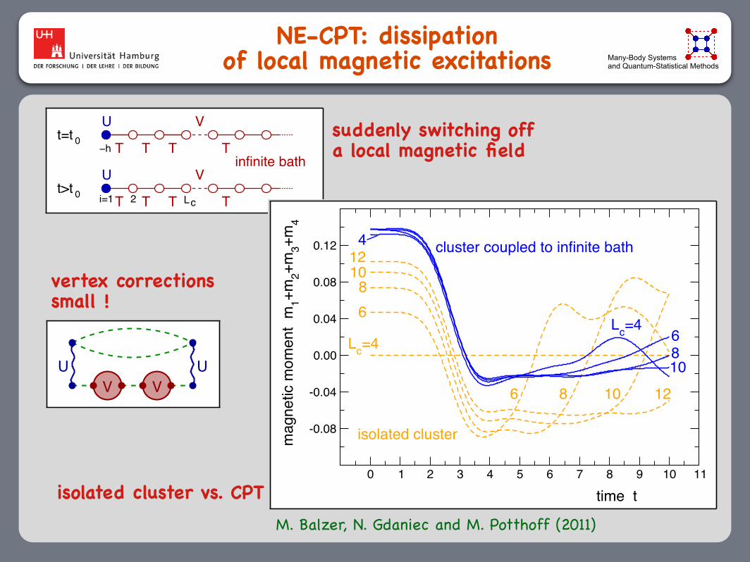
NE-CPT: dissipation of local magnetic excitations Many-Body Systems
and Quantum-Statistical Methods
vertex corrections!small !
Non-equilibrium self-energy-functional theory Ringberg Castle, 12.9.2011—————————————————————————————————————————————————————————–˛
˛
˛
˛
˛
˛
˛
˛
˛
˛
NE-CPT: dissipation of local magnetic excitation
U
U
0t>tV
i=1 2 TT T
V
T TT−h0t=t
T
Lc T
infinite bath
small vertex corrections:
V VUU
dissipation physics:
0 1 2 3 4 5 6 7 8 9 10 11
-0.08
-0.04
0.00
0.04
0.08
0.12
mag
netic
mom
ent
m1+m
2+m3+m
4
time t
cluster coupled to infinite bath
isolated cluster
Lc=4
6
108
4
Lc=4
12
6810
8 10 126
. – p.15
isolated cluster vs. CPT
suddenly switching off !a local magnetic field
M. Balzer, N. Gdaniec and M. Potthoff (2011)
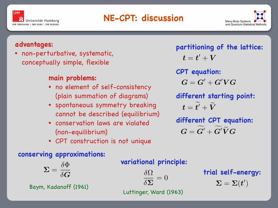
NE-CPT: discussion Many-Body Systems and Quantum-Statistical Methods
main problems:!• no element of self-consistency
(plain summation of diagrams)!• spontaneous symmetry breaking
cannot be described (equilibrium)!• conservation laws are violated
(non-equilibrium)!• CPT construction is not unique
t = t0 + V
CPT equation:
t = et0 + eV
G = fG0 + fG0 eV G
G = G0 +G0V G
partitioning of the lattice:
different starting point:
different CPT equation:
advantages:!• non-perturbative, systematic,
conceptually simple, flexible
conserving approximations:
=
G
Baym, Kadanoff (1961)
variational principle:!
= 0
Luttinger, Ward (1963) = (t0)
trial self-energy:
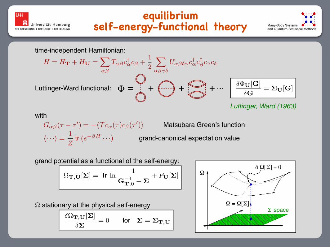
equilibrium self-energy-functional theory Many-Body Systems
and Quantum-Statistical Methods
Kondo screening
Non-equilibrium self-energy-functional theory Ringberg Castle, 12.9.2011—————————————————————————————————————————————————————————–˛
˛
˛
˛
˛
˛
˛
˛
˛
˛
equilibrium self-energy-functional theory
time-independent Hamiltonian:H = HT + HU =
X
αβ
Tαβc†αcβ +1
2
X
αβγδ
Uαβδγc†αc†βcγcδ
Luttinger-Ward functional: = + + +ΦδΦU[G]
δG= ΣU[G]
Luttinger, Ward (1963)with
Gαβ(τ − τ ′) = −⟨cα(τ)c†β(τ ′)⟩ Matsubara Green’s function
⟨· · ·⟩ =1
Ztr (e−βH · · ·) grand-canonical expectation value
grand potential as a functional of the self-energy:
ΩT,U[Σ] = Tr ln1
G−1T,0 − Σ
+ FU[Σ]
Ω stationary at the physical self-energyδΩT,U[Σ]
δΣ= 0 for Σ = ΣT,U
Σ space
Ω
Ω = Ω[Σ]
δ Ω[Σ] = 0
. – p.3
= hT c↵()c(0)i
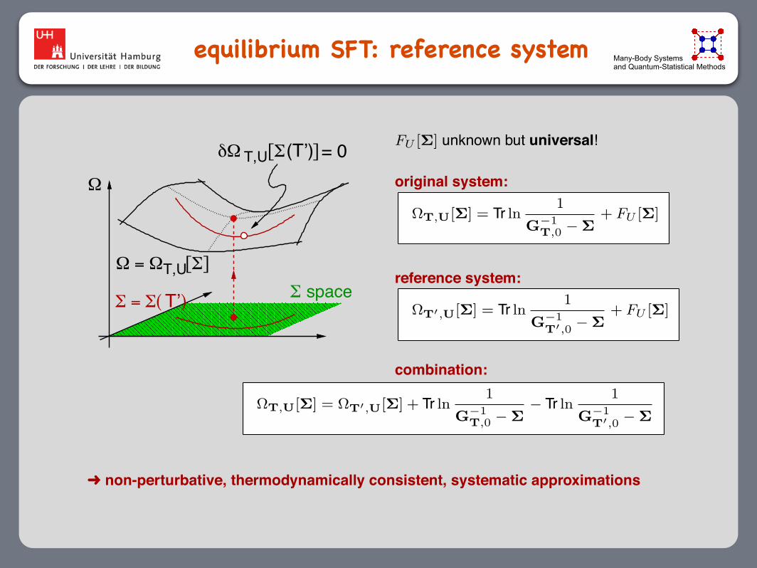
equilibrium SFT: reference system Many-Body Systems and Quantum-Statistical Methods
Non-equilibrium self-energy-functional theory Ringberg Castle, 12.9.2011—————————————————————————————————————————————————————————–˛
˛
˛
˛
˛
˛
˛
˛
˛
˛
equilibrium SFT: reference system
Ω
Σ space
= 0(T’)δΩ [Σ ]T,U
T,UΩ = Ω [Σ]
Σ = Σ( )T’
FU [Σ] unknown but universal!
original system:
ΩT,U[Σ] = Tr ln 1
G−1T,0 − Σ
+ FU [Σ]
reference system:
ΩT′,U[Σ] = Tr ln 1
G−1T′,0
− Σ+ FU [Σ]
combination:
ΩT,U[Σ] = ΩT′,U[Σ] + Tr ln 1
G−1T,0 − Σ
− Tr ln 1
G−1T′,0 − Σ
non-perturbative, thermodynamically consistent, systematic approximations
. – p.4
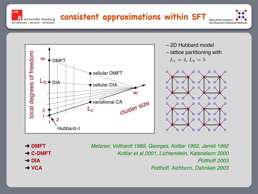
consistent approximations within SFT Many-Body Systems and Quantum-Statistical MethodsNon-equilibrium self-energy-functional theory Ringberg Castle, 12.9.2011—————————————————————————————————————————————————————————–˛
˛
˛
˛
˛
˛
˛
˛
˛
˛
consistent approximations within SFTlo
cal d
egre
es o
f fre
edom
cluster size
oo
1 2
Lc
Hubbard−I
DIA cellular DIA
variational CA
oo DMFT
cellular DMFT
21
bL
– 2D Hubbard model– lattice partitioning with
Lc = 4, Lb = 5
DMFT Metzner, Vollhardt 1989, Georges, Kotliar 1992, Jarrell 1992 C-DMFT Kotliar et al 2001, Lichtenstein, Katsnelson 2000 DIA Potthoff 2003 VCA Potthoff, Aichhorn, Dahnken 2003
. – p.5

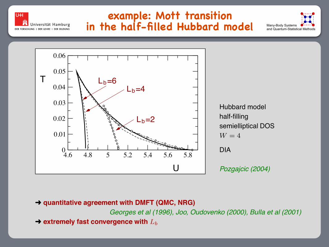
example: Mott transition !in the half-filled Hubbard model Many-Body Systems
and Quantum-Statistical Methods
0 0.1 0.2 0.3 0.4
-2.708
-2.706
-2.704
-2.702
-2.7
-2.698
-2.696
-2.694
V
Ω
U=5.2
0.004
0.002
0.006
0.008
0.010
0.012
0.014
0.016
0.018
0.020
T=0
4.6 4.8 5 5.2 5.4 5.6 5.8 6
0
0.01
0.02
0.03
0.04
UcUc1 Uc2
metal insulator
coex.
Tc
U
T crossover
0 2 4 6 80.0
0.2
0.4
0.6
0.8
1.0
U
z(U) BR2-site DMFT
DIA, ns=2DIA, ns=4
DIA, ns=oo
Potthoff (2003)
original and reference system grand potential vs. variational parameterVariants of DMFT FZ Jülich, 5.7.2007—————————————————————————————————————————————————————————–˛
˛
˛
˛
˛
˛
˛
˛
˛
˛
two-site DMFT
two-site impurity model:
εbath
εcV
3 (2) parameters to be determined
DMFT self-consistency condition: Gloc(ω) = G(ω)
3) high-frequency expansion of coherent part
z
0ω
DOS
G(coh)loc (ω) = G(coh)(ω)
z = 1/(1 − Σ′(0))
· · · +z3(M2 + (t0 − µ + a)2)
ω3+ · · · = · · · +
z2V 2 + z3(εc − µ + a)2)
ω3+ · · ·
second self-consistency conditions of two-site DMFT: M2 =1
L
X
k
ε(k)2 =X
j
t2ij
zM2 = V 2
. – p.8
mean-field phase diagram
DIA vs. DMFT
(DMFT)
example: Mott transition !in the half-filled Hubbard model Many-Body Systems
and Quantum-Statistical Methods
Variants of DMFT FZ Jülich, 5.7.2007—————————————————————————————————————————————————————————–˛
˛
˛
˛
˛
˛
˛
˛
˛
˛
finite-temperature Mott transition
4.6 4.8 5 5.2 5.4 5.6 5.80
0.01
0.02
0.03
0.04
0.05
0.06
N=6N=4N=2L =6 b
L =4b
L =2b
T
U
Hubbard modelhalf-fillingsemielliptical DOSW = 4
DIA
Pozgajcic (2004)
quantitative agreement with DMFT (QMC, NRG)Georges et al (1996), Joo, Oudovenko (2000), Bulla et al (2001)
extremely fast convergence with Lb
. – p.21
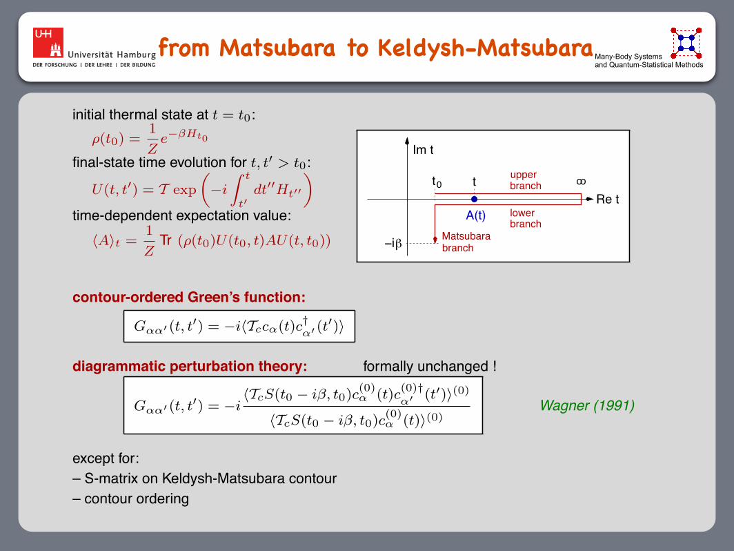
from Matsubara to Keldysh-MatsubaraMany-Body Systems and Quantum-Statistical Methods
Non-equilibrium self-energy-functional theory Ringberg Castle, 12.9.2011—————————————————————————————————————————————————————————–˛
˛
˛
˛
˛
˛
˛
˛
˛
˛
from Matsubara to Keldysh-Matsubara
initial thermal state at t = t0:ρ(t0) =
1
Ze−βHt0
final-state time evolution for t, t′ > t0:
U(t, t′) = T exp
„
−i
Z t
t′dt′′Ht′′
«
time-dependent expectation value:⟨A⟩t =
1
ZTr (ρ(t0)U(t0, t)AU(t, t0))
oo
Im t
t t0
Matsubara
Re t
β−i
lower
upperbranch
branch
branch
A(t)
contour-ordered Green’s function:
Gαα′ (t, t′) = −i⟨Tccα(t)c†α′ (t
′)⟩
diagrammatic perturbation theory: formally unchanged !
Gαα′ (t, t′) = −i⟨TcS(t0 − iβ, t0)c
(0)α (t)c
(0)†α′ (t′)⟩(0)
⟨TcS(t0 − iβ, t0)c(0)α (t)⟩(0)
Wagner (1991)
except for:– S-matrix on Keldysh-Matsubara contour– contour ordering
. – p.6

NON-EQUILIBRIUM self-energy functional theory Many-Body Systems
and Quantum-Statistical Methods
Non-equilibrium self-energy-functional theory Ringberg Castle, 12.9.2011—————————————————————————————————————————————————————————–˛
˛
˛
˛
˛
˛
˛
˛
˛
˛
NON-EQUILIBRIUM self-energy-functional theory
TIME-DEPENDENT Hamiltonian:Ht = HT(t) + HU(t) =
X
αβ
Tαβ(t)c†αcβ +1
2
X
αβγδ
Uαβδγ(t)c†αc†βcγcδ
Luttinger-Ward functional: = + + +ΦδΦU[G]
δG= ΣU[G]
withGαα′ (t, t′) = −i⟨cα(t)c†
α′ (t′)⟩ CONTOUR-ORDERED Green’s function
⟨· · ·⟩ =1
Ztr (e−βHt0 · · ·) grand-canonical expectation value
INITIAL-STATE grand potential:
ΩT,U[Σ] = Tr ln1
G−1T,0 − Σ
+ FU[Σ]
Ω stationary at the physical self-energyδΩT,U[Σ]
δΣ= 0 for Σ = ΣT,U
Σ space
Ω
Ω = Ω[Σ]
δ Ω[Σ] = 0
. – p.7
= ihT c↵(t)c↵0(t0)i†

NON-EQUILIBRIUM SFT: reference system Many-Body Systems
and Quantum-Statistical MethodsNon-equilibrium self-energy-functional theory Ringberg Castle, 12.9.2011—————————————————————————————————————————————————————————–˛
˛
˛
˛
˛
˛
˛
˛
˛
˛
NON-EQUILIBRIUM SFT: reference system
Ω
Σ space
= 0(T’)δΩ [Σ ]T,U
T,UΩ = Ω [Σ]
Σ = Σ( )T’
FU [Σ] unknown but universal!
original system:
ΩT,U[Σ] = Tr ln 1
G−1T,0 − Σ
+ FU [Σ]
reference system:
ΩT′,U[Σ] = Tr ln 1
G−1T′,0
− Σ+ FU [Σ]
combination:
ΩT,U[Σ] = ΩT′,U[Σ] + Tr ln 1
G−1T,0 − Σ
− Tr ln 1
G−1T′,0 − Σ
non-perturbative, thermodynamically consistent, systematic approximations
. – p.8
Hofmann, Eckstein, Arrigoni, Potthoff (2013)

NE-SFT: consistent approximations Many-Body Systems and Quantum-Statistical Methods
Non-equilibrium self-energy-functional theory Ringberg Castle, 12.9.2011—————————————————————————————————————————————————————————–˛
˛
˛
˛
˛
˛
˛
˛
˛
˛
consistent approximations within NE-SFTlo
cal d
egre
es o
f fre
edom
cluster sizeoo
1 2
Lc
NE Hubbard−I
NE DIA NE cellular DIA
NE variational CA
oo
NE cellular DMFT
NE DMFT
21
bL
Lc = 4, ns = 5
NE-DMFT Freericks, Turkowski, Zlatic (2007), Schmidt, Monien (2002) NE-VCA Balzer, Potthoff (2011), Jung et al. (2011), Knap et al. (2011)
no parameter optimization:non-equilibrium cluster-perturbation theory (NE-CPT)
. – p.9
NE-DMFTNE-VCA/CPT

variational optimization !of time-dependent parameters Many-Body Systems
and Quantum-Statistical Methods
• trial self-energy from reference system with parameters T’=T(z), varied by variation of T’(z)!
• independent variations T+(t) and T-(t) on the upper/lower Keldysh branch
Non-equilibrium self-energy-functional theory Ringberg Castle, 12.9.2011—————————————————————————————————————————————————————————–˛
˛
˛
˛
˛
˛
˛
˛
˛
˛
from Matsubara to Keldysh-Matsubara
initial thermal state at t = t0:ρ(t0) =
1
Ze−βHt0
final-state time evolution for t, t′ > t0:
U(t, t′) = T exp
„
−i
Z t
t′dt′′Ht′′
«
time-dependent expectation value:⟨A⟩t =
1
ZTr (ρ(t0)U(t0, t)AU(t, t0))
oo
Im t
t t0
Matsubara
Re t
β−i
lower
upperbranch
branch
branch
A(t)
contour-ordered Green’s function:
Gαα′ (t, t′) = −i⟨Tccα(t)c†α′ (t
′)⟩
diagrammatic perturbation theory: formally unchanged !
Gαα′ (t, t′) = −i⟨TcS(t0 − iβ, t0)c
(0)α (t)c
(0)†α′ (t′)⟩(0)
⟨TcS(t0 − iβ, t0)c(0)α (t)⟩(0)
Wagner (1991)
except for:– S-matrix on Keldysh-Matsubara contour– contour ordering
. – p.6
physical and transverse variations
T0phys(t) =
1
2(T0
+(t) +T0(t))
T0trans(t) =
1
2(T0
+(t)T0(t))T0
phys(t) =1
2(T0
+(t) +T0(t))
T0trans(t) =
1
2(T0
+(t)T0(t))
T0+
T0
T0trans
T0
trans=0
!= 0 (fixes T0
phys)
T0phys
T0
trans=0
= 0 (trivially)
trans.phys.
p
h
y
s
i
c
a
l
m
a
n
i
f
o
l
d
T0trans(t)
=0
• stationarity w.r.t. physical variations: solutions are “physical”(follows trivially from cancellation of forward and backward time evolution)!
• SFT functional, evaluated at physical parameters, depends on the self-energy on the Matsubara branch only!
• stationarity w.r.t. transverse variations: fixes the solution on the physical manifold
’ ’
HOFMANN, ECKSTEIN, ARRIGONI, AND POTTHOFF PHYSICAL REVIEW B 88, 165124 (2013)
−βΦ = + + + . . .
FIG. 2. Diagrammatic definition of the Luttinger-Ward functional!!U [G]. Double lines: fully interacting propagator G. Dashed lines:interaction U . See text for discussion.
the “free” density operator exp(−βHT ,0)/ tr exp(−βHT ,0).Hence, Wick’s theorem applies and therewith the standardtechniques of perturbation theory.53
III. LUTTINGER-WARD FUNCTIONAL
The nonequilibrium Luttinger-Ward functional !!U [G] canbe defined by means of all-order perturbation theory inclose analogy to the equilibrium case.57 It is obtained as thelimit of the infinite series of closed renormalized skeletondiagrams (see Fig. 2), and is thus given as a functional of thecontour-ordered Green’s function. Note that functionals areindicated by a hat. Usually, the skeleton-diagram expansioncan not be summed up to get a closed form for !!U [G], and theexplicit functional dependence is unknown even for the mostsimple types of interactions like the Hubbard interaction. Asan alternative to the diagrammatic definition of the Luttinger-Ward functional, a nonequilibrium path-integral formalismmay be used for an entirely nonperturbative construction.Again, this can be done analogously to the equilibriumcase.58 Both variants allow us to derive the following fourproperties that will be used extensively for constructing thenonequilibrium SFT:
(i) The Luttinger-Ward functional vanishes in the nonin-teracting limit
!!U [G] ≡ 0 for U = 0 (11)
since there is no zeroth-order diagram.(ii) The functional derivative of the Luttinger-Ward func-
tional with respect to its argument is
δ!!U [G]δG(1,2)
= 1β
!$U [G](2,1) (12)
with the shorthand notation i ≡ (αi ,zi). Diagrammatically,the functional derivative corresponds to the removal of apropagator from each of the ! diagrams. Taking care oftopological factors,57 one ends up with the skeleton-diagramexpansion of the self-energy which, independently from thedefinition [Eq. (8)] gives the self-energy as a functional of theGreen’s function !!U [G]. Evaluating the functional !! at theexact (“physical”) Green’s function GT ,U yields the physicalself-energy
!!U [GT ,U ] = !T ,U . (13)
(iii) Since any diagram in the series depends on U and onG only, the Luttinger-Ward functional is “universal,” i.e., it isindependent of T . Two systems with the same interaction U butdifferent one-particle parameters T are described by the sameLuttinger-Ward functional. This implies that the functional!!U [G] is universal, too.
(iv) If evaluated at the physical Green’s function GT ,U of thesystem with Hamiltonian HT ,U , the Luttinger-Ward functionalprovides a quantity
!!U [GT ,U ] = !T ,U . (14)
Note that !T ,U depends on the initial equilibrium state of thesystem only, as contributions from the Keldysh branch canceleach other (for details, see Sec. VII). !T ,U is related to thegrand potential of the system via the expression
&T ,U = !T ,U + 1β
Tr ln"G−1
ε0,0 GT ,U#
− 1β
Tr(!T ,U GT ,U ). (15)
Here, we defined the trace as
Tr A =$
α
%
Cdz Aαα(z,z+), (16)
where z+ is infinitesimally later than z on C. The factor G−1ε0,0
with ε0 → ∞ has to be introduced to regularize the Tr ln termas discussed in Appendix A. It will be omitted in the followingas it does not affect the results. Equation (15) can be derivedusing a coupling-constant integration57 or by integrating overthe chemical potential µ.58 The proof is completely analogousto the equilibrium case.
IV. DYNAMICAL VARIATIONAL PRINCIPLE
We assume the functional !!U [G] is invertible locallyto construct the Legendre transform of the Luttinger-Wardfunctional
!FU [!] = !!U [!GU [!]] − 1β
Tr(! !GU [!]). (17)
Here, !GU [!!U [G]] = G. With Eq. (12), one has
δ!FU [!]δ$(1,2)
= − 1β
!GU [!](2,1). (18)
We now define the self-energy functional as
!&T ,U [!] = 1β
Tr ln"G−1
T ,0 − !#−1 + !FU [!]. (19)
Its functional derivative is [use Eq. (A2)]
δ!&T ,U [!]δ!
= 1β
"G−1
T ,0 − !#−1 − 1
β!GU [!]. (20)
The equation
!GU [!] ="G−1
T ,0 − !#−1 (21)
is a (highly nonlinear) conditional equation for the self-energyof the system HT ,U . Equations (8) and (13) show that it issatisfied by the physical self-energy ! = !T ,U . Note that theleft-hand side of Eq. (21) is independent of T but depends onU (due to the universality of !GU [!]), while the right-handside is independent of U but depends on T via G−1
T ,0.The obvious problem of finding a solution of Eq. (21) is
that there is no closed form for the functional !GU [!]. Solving
165124-4
NON-EQUILIBRIUM self-energy functional theory Many-Body Systems
and Quantum-Statistical Methods
Non-equilibrium self-energy-functional theory Ringberg Castle, 12.9.2011—————————————————————————————————————————————————————————–˛
˛
˛
˛
˛
˛
˛
˛
˛
˛
NON-EQUILIBRIUM self-energy-functional theory
TIME-DEPENDENT Hamiltonian:Ht = HT(t) + HU(t) =
X
αβ
Tαβ(t)c†αcβ +1
2
X
αβγδ
Uαβδγ(t)c†αc†βcγcδ
Luttinger-Ward functional: = + + +ΦδΦU[G]
δG= ΣU[G]
withGαα′ (t, t′) = −i⟨cα(t)c†
α′ (t′)⟩ CONTOUR-ORDERED Green’s function
⟨· · ·⟩ =1
Ztr (e−βHt0 · · ·) grand-canonical expectation value
INITIAL-STATE grand potential:
ΩT,U[Σ] = Tr ln1
G−1T,0 − Σ
+ FU[Σ]
Ω stationary at the physical self-energyδΩT,U[Σ]
δΣ= 0 for Σ = ΣT,U
Σ space
Ω
Ω = Ω[Σ]
δ Ω[Σ] = 0
. – p.7
= ihT c↵(t)c↵0(t0)i

variational optimization !of time-dependent parameters Many-Body Systems
and Quantum-Statistical Methods
Non-equilibrium self-energy-functional theory Ringberg Castle, 12.9.2011—————————————————————————————————————————————————————————–˛
˛
˛
˛
˛
˛
˛
˛
˛
˛
NON-EQUILIBRIUM SFT: reference system
Ω
Σ space
= 0(T’)δΩ [Σ ]T,U
T,UΩ = Ω [Σ]
Σ = Σ( )T’
FU [Σ] unknown but universal!
original system:
ΩT,U[Σ] = Tr ln 1
G−1T,0 − Σ
+ FU [Σ]
reference system:
ΩT′,U[Σ] = Tr ln 1
G−1T′,0
− Σ+ FU [Σ]
combination:
ΩT,U[Σ] = ΩT′,U[Σ] + Tr ln 1
G−1T,0 − Σ
− Tr ln 1
G−1T′,0 − Σ
non-perturbative, thermodynamically consistent, systematic approximations
. – p.8
T0phys(t) =
1
2(T0
+(t) +T0(t))
T0trans(t) =
1
2(T0
+(t)T0(t))
T0+
T0
T0trans
T0
trans=0
!= 0 (fixes T0
phys)
T0phys
T0
trans=0
= 0 (trivially)
trans.phys.
p
h
y
s
i
c
a
l
m
a
n
i
f
o
l
d
T0trans(t)
=0
• equilibrium SFT: compute SFT functional at trial self-energyfind stationary point of the function!
• non-equilibrium SFT: carry out functional derivative analytically numerical solution of resulting Euler equation!
T 0 7! [(T 0)]

NE SFT Euler equation Many-Body Systems and Quantum-Statistical Methods
HOFMANN, ECKSTEIN, ARRIGONI, AND POTTHOFF PHYSICAL REVIEW B 88, 165124 (2013)
as a set of decoupled single-impurity Anderson models. ForLc = 1, the trial self-energies are local, i.e., diagonal with
respect to the spatial indices, and the Euler equation (26) thusexplicitly reads as
0 = δ!"T ,U [!λ′,U ]δλ′(z)
= 1β
"
i,σ1σ2
#
Cdz1dz2
$%G−1
T ,0−!λ′,U&−1− Gλ′,U
'ii,σ1σ2
(z1,z2)δ%λ′,U ;ii,σ2σ1 (z2,z
+1 )
δλ′(z). (28)
Here, i is a site index and σi refers to the local orbital and spindegrees of freedom.
Equation (28) would be trivially satisfied if the squarebrackets in the integrand vanished. Because the vanishing ofthe square brackets is nothing but the standard self-consistencyequation of DMFT,18–20 we see that nonequilibrium SFTyields (nonequilibrium) DMFT as a stationary point, providedthat the DMFT self-energy can be represented as the self-energy !λ′,U of a single-impurity Anderson Hamiltonian withsingle-particle (bath) parameters λ′. The representability ofthe DMFT action by an actual impurity Hamiltonian withLb = ∞ is not straightforward to see for nonequilibriumGreen’s functions, but can be shown under rather generalconditions.38
When one considers finite single-impurity models with asmall number of bath orbitals, the square brackets in Eq. (28)will in general not vanish because the discrete pole structure ofthe impurity Green’s function can not be reconciled with thebranch cuts of the Green’s function for the original model. Dueto the presence of the projector δ%λ′/δλ′, however, stationarityof the self-energy functional is nevertheless possible. Thisallows us to generate nonperturbative and consistent approx-imations to DMFT by solving reference systems with a fewdegrees of freedom only. In the equilibrium case, this has beenshown to be a highly efficient strategy (see, e.g., Refs. 33and 34).
VII. PHYSICAL AND TRANSVERSE VARIATIONS
The variational problem [Eq. (26)] is posed on the wholecontour C, i.e., the self-energy functional must be stationarywith respect to variations of the parameters λ′(z) separatelyon the Matsubara branch and on both branches of theKeldysh contour. This generates one imaginary-time and twoindependent real-time Euler equations which are obtained bywriting !"T ,U [!λ′,U ] ≡ !"T ,U [!λ′
+,λ′−,λ′
M,U ] as a functional ofthe single-particle parameters λ±(t) on the upper/lower branchof the contour (for real t), as well as of the parameters λ′
M(t0 −iτ ) on the Matsubara branch. Using a simple transformationof variables,
λ′phys(t) = 1
2 [λ′+(t) + λ′
−(t)],(29)
λ′trans(t) = 1
2 [λ′+(t) − λ′
−(t)],
the real-time equations become equivalent toδ!"T ,U [!λ′
phys,λ′trans,λ
′M,U ]/δλ′
phys/trans(t) = 0.The separation into variations with respect to λ′
phys (“physi-cal variations”) and λ′
trans (“transverse variations”) has a simplemotivation: In the end, we are only interested in solutions ofthe Euler equation by a physical parameter set λ′(z), i.e., onethat corresponds to an actual Hamiltonian. These parameters
must thus satisfy λ′+(t) = λ′
−(t), i.e., λ′trans(t) = 0. In addition,
λ′M (t0 − iτ ) must not depend on imaginary time (this is
discussed in Sec. IX). Transverse variations δλ′trans(t) = 0
shift the parameters away from the physical manifold, whilephysical variations remain therein.
Let us first consider variations of λ′phys(t). Interestingly, one
can show that the self-energy functional is always stationarywith respect to physical variations when evaluated at a physicalparameter set, which satisfies λ′
trans(t) = 0, i.e.,
δ!"T ,U$!λ′
phys,λ′trans,λ
′M,U
'
δλ′phys(t)
(((((λ′
trans(t)=0
= 0. (30)
To prove Eq. (30), we first note that any Green’s functiondefined by Eq. (6) is symmetric with respect to a shift of thelargest time argument on the Keldysh contour from the upperto the lower branch, i.e.,
X(t0 − iτ,t+) = X(t0 − iτ,t−),(31)
X(t ′,t+) = X(t ′,t−) for t > t ′,
and similar for the first time argument (t± denotes a time argu-ment on the upper/lower branch at t). This symmetry relation,which is often formulated as a fundamental relation betweenbetween retarded, advanced, and time-ordered components ofthe Green’s functions,54 immediately follows from the factthat the forward and backward time evolutions cancel eachother after the rightmost operator on the Keldysh contour (seealso the discussion of Fig. 1). The same property holds for theconvolution A B of any two contour functions A and B ifit holds for A and B individually, and thus for any functionof X [cf. Eq. (A1)]. Furthermore, it is easy to see that in theexpression (16) for the trace all integrations over the Keldyshbranch cancel for any function with the symmetry (31). Thus,the self-energy functional (19), when evaluated at physicalparameters, depends on the Matsubara part of !λ′,U only. Thisimmediately implies the stationarity condition (30).
Stationarity with respect to physical variations locallyrestricts the solution to the physical manifold. Thus, a secondequation is needed to fix the solution within the physicalmanifold. This “second” equation is given by the conditionthat the self-energy functional be stationary with respect to thetransverse variations, if evaluated at a physical parameter set:
δ!"T ,U$!λ′
phys,λ′trans,λ
′M,U
'
δλ′trans(t)
(((((λ′
trans(t)=0
= 0. (32)
Equation (32) is the central equation of the nonequilibriumSFT.
Let us stress once more that the functional derivativewith respect to λ′
trans(t) is a derivative into a “nonphysical”
165124-6
NONEQUILIBRIUM SELF-ENERGY FUNCTIONAL THEORY PHYSICAL REVIEW B 88, 165124 (2013)
direction in parameter space. This has important conceptualconsequences for the numerical evaluation of the theory. Inthe vast majority of previous equilibrium SFT studies, thegrand potential !!T ,U [!λ′,U ] has been computed for different(static) parameter sets λ′, and algorithms to find a stationarypoint of a multidimensional scalar function λ′ "→ !!T ,U [!λ′,U ]have been employed (see Ref. 59, for example). In thenonequilibrium case, a similar strategy would require us towork explicitly with Green’s functions that are defined witha different Hamiltonian for the forward and backward timeevolutions. A more convenient strategy, which is worked outin the following, is to carry out the functional derivativeanalytically and to solve the resulting Euler equation bynumerical means. The analytical expressions for the functionalderivatives are then given by higher-order correlation functionsevaluated at the physical parameters.
VIII. EVALUATION OF THE EULER EQUATION
We focus on Eq. (25) again and perform the functionalderivative in Eq. (26) analytically. This is most convenientlydone by considering the variational parameters as functions ofthe contour variable, i.e., λ′(z) with z ∈ C, instead of treatingλ±(t) and λM(t0 − iτ ) separately.
Using the chain rule, we find
δ!!T ,U [!λ′,U ]δλ′
α1α2(z)
= Tr
"δ!!T ,U [!λ′,U ]
δ!λ′,U δ!λ′,U
δλ′α1α2
(z)
#
. (33)
The first factor is given by Eq. (20) but can be rewritten in amore convenient way. We define the difference between theone-particle parameters of the original and of the referencesystem as
V (z) = T (z) − λ′(z). (34)
With this, we immediately have [see Eq. (7)]
G−1λ′,0(1,2) = G−1
T ,0(1,2) + δC(z1,z2)Vα1α2 (z2). (35)
Here, we use the standard notation 1 ≡ (α1,z1), etc. With thedefinition of the SFT Green’s function [Eq. (27)] and withDyson’s equation for the reference system, we get
GSFT = Gλ′,U + Gλ′,U V GSFT. (36)
This equation constitutes the nonequilibrium cluster-perturbation theory.39 One may formally consider perturbationtheory with respect to V and define the corresponding T matrixas
Yλ′,T ,U (z1,z2) = V (z1)δC(z1,z2)
+ V (z1)GSFT(z1,z2)V (z2). (37)
The related Lippmann-Schwinger equation is
GSFT = Gλ′,U + Gλ′,U Yλ′,T ,U Gλ′,U . (38)
This eventually yields
δ!!T ,U [!λ′,U ]δ!λ′,U
= 1β
Gλ′,U Yλ′,T ,U Gλ′,U (39)
for the first factor in Eq. (33).To evaluate the second factor, the Dyson equation for
the reference system is used once more to get !λ′,U =
G−1λ′,0 − G−1
λ′,U . The λ′ dependence of the inverse freeGreen’s function is simple: G−1
λ′,0(1,2) = δC(z1,z2)δα1,α2 i∂z2 −δC(z1,z2)[λ′
α1α2(z2) − δα1α2µ]. We thus get
δ(λ′,U (3,4)δλ′
α1α2(z1)
= −δC(z3,z4)δα3α1δC(z4,z1)δα4α2
+$$
d5 d6 G−1λ′,U (3,5)
δGλ′,U (5,6)δλ′
α1α2(z1)
G−1λ′,U (6,4). (40)
The functional derivative of the Green’s function is computedin the Appendix B and given by Eq. (B2).
Combining this with Eq. (39), we finally get the derivativeof the self-energy functional with respect to λ′(z1) in the form
δ!!T ,U [!λ′,U ]δλ′
α1α2(z1)
= − 1β
$$d3 d4Yλ′,T ,U (4,3)Lλ′,U (3,2,1+,4)|z2=z1 , (41)
where
Lλ′,U (1,2,3,4) = Gλ′,U (2,4)Gλ′,U (1,3)
−Gλ′,U (1,4)Gλ′,U (2,3) + G(2)λ′,U (1,2,3,4)
(42)
is the two-particle (four-point) vertex function with externallegs and G(2)
λ′,U is the two-particle Green’s function of thereference system [see Eq. (B3)].
Therewith, we have the Euler equation of the nonequilib-rium SFT:$$
d3 d4 Yλ′opt,T ,U (4,3)Lλ′
opt,U (3,2,1+,4)|z2=z1 = 0. (43)
This result will be needed both for the numerical determinationof the stationary point and for working out the relation betweennonequilibrium and conventional equilibrium SFT.
IX. THERMAL EQUILIBRIUM AND INITIAL STATE
Nonequilibrium SFT reduces to the conventional equilib-rium formalism for a system where T (z) and U(z) are constanton the entire contour C, i.e., for the case Hfin(t) = const = Hini.To prove this fact explicitly, we have to show that a stationarypoint of the equilibrium SFT functional, which determinestime-independent optimal parameters λ′
opt, is also a stationarypoint of the more general nonequilibrium Euler equation (26),i.e., of Eq. (43), when T (z) and U(z) are constant.
Equilibrium SFT is obtained from the more generalnonequilibrium formalism by restricting the functional (25)to the Matsubara branch of the contour and, furthermore, byconsidering time-independent and physical variations only,i.e., the trial self-energy !λ′,U is obtained as the Matsubaraself-energy of a Hamiltonian with constant parameters λ′, andthe parameters are varied to make !!T ,U [!λ′,U ] stationary.In the language of the more general nonequilibrium SFTformalism, those variations correspond to a variation δλ(z)which is constant along the whole contour, i.e.,
∂!!T ,U [!λ′,U ]∂λ′ =
$
Cdz
δ!!T ,U [!λ′,U ]δλ′(z)
. (44)
165124-7
Euler equation to fix physical variational parameters
connected two-particle Green’s function of the reference systemT-matrix of perturbation theory
in V (inter-cluster hopping)

causality and propagation scheme Many-Body Systems and Quantum-Statistical Methods
HOFMANN, ECKSTEIN, ARRIGONI, AND POTTHOFF PHYSICAL REVIEW B 88, 165124 (2013)
as a set of decoupled single-impurity Anderson models. ForLc = 1, the trial self-energies are local, i.e., diagonal with
respect to the spatial indices, and the Euler equation (26) thusexplicitly reads as
0 = δ!"T ,U [!λ′,U ]δλ′(z)
= 1β
"
i,σ1σ2
#
Cdz1dz2
$%G−1
T ,0−!λ′,U&−1− Gλ′,U
'ii,σ1σ2
(z1,z2)δ%λ′,U ;ii,σ2σ1 (z2,z
+1 )
δλ′(z). (28)
Here, i is a site index and σi refers to the local orbital and spindegrees of freedom.
Equation (28) would be trivially satisfied if the squarebrackets in the integrand vanished. Because the vanishing ofthe square brackets is nothing but the standard self-consistencyequation of DMFT,18–20 we see that nonequilibrium SFTyields (nonequilibrium) DMFT as a stationary point, providedthat the DMFT self-energy can be represented as the self-energy !λ′,U of a single-impurity Anderson Hamiltonian withsingle-particle (bath) parameters λ′. The representability ofthe DMFT action by an actual impurity Hamiltonian withLb = ∞ is not straightforward to see for nonequilibriumGreen’s functions, but can be shown under rather generalconditions.38
When one considers finite single-impurity models with asmall number of bath orbitals, the square brackets in Eq. (28)will in general not vanish because the discrete pole structure ofthe impurity Green’s function can not be reconciled with thebranch cuts of the Green’s function for the original model. Dueto the presence of the projector δ%λ′/δλ′, however, stationarityof the self-energy functional is nevertheless possible. Thisallows us to generate nonperturbative and consistent approx-imations to DMFT by solving reference systems with a fewdegrees of freedom only. In the equilibrium case, this has beenshown to be a highly efficient strategy (see, e.g., Refs. 33and 34).
VII. PHYSICAL AND TRANSVERSE VARIATIONS
The variational problem [Eq. (26)] is posed on the wholecontour C, i.e., the self-energy functional must be stationarywith respect to variations of the parameters λ′(z) separatelyon the Matsubara branch and on both branches of theKeldysh contour. This generates one imaginary-time and twoindependent real-time Euler equations which are obtained bywriting !"T ,U [!λ′,U ] ≡ !"T ,U [!λ′
+,λ′−,λ′
M,U ] as a functional ofthe single-particle parameters λ±(t) on the upper/lower branchof the contour (for real t), as well as of the parameters λ′
M(t0 −iτ ) on the Matsubara branch. Using a simple transformationof variables,
λ′phys(t) = 1
2 [λ′+(t) + λ′
−(t)],(29)
λ′trans(t) = 1
2 [λ′+(t) − λ′
−(t)],
the real-time equations become equivalent toδ!"T ,U [!λ′
phys,λ′trans,λ
′M,U ]/δλ′
phys/trans(t) = 0.The separation into variations with respect to λ′
phys (“physi-cal variations”) and λ′
trans (“transverse variations”) has a simplemotivation: In the end, we are only interested in solutions ofthe Euler equation by a physical parameter set λ′(z), i.e., onethat corresponds to an actual Hamiltonian. These parameters
must thus satisfy λ′+(t) = λ′
−(t), i.e., λ′trans(t) = 0. In addition,
λ′M (t0 − iτ ) must not depend on imaginary time (this is
discussed in Sec. IX). Transverse variations δλ′trans(t) = 0
shift the parameters away from the physical manifold, whilephysical variations remain therein.
Let us first consider variations of λ′phys(t). Interestingly, one
can show that the self-energy functional is always stationarywith respect to physical variations when evaluated at a physicalparameter set, which satisfies λ′
trans(t) = 0, i.e.,
δ!"T ,U$!λ′
phys,λ′trans,λ
′M,U
'
δλ′phys(t)
(((((λ′
trans(t)=0
= 0. (30)
To prove Eq. (30), we first note that any Green’s functiondefined by Eq. (6) is symmetric with respect to a shift of thelargest time argument on the Keldysh contour from the upperto the lower branch, i.e.,
X(t0 − iτ,t+) = X(t0 − iτ,t−),(31)
X(t ′,t+) = X(t ′,t−) for t > t ′,
and similar for the first time argument (t± denotes a time argu-ment on the upper/lower branch at t). This symmetry relation,which is often formulated as a fundamental relation betweenbetween retarded, advanced, and time-ordered components ofthe Green’s functions,54 immediately follows from the factthat the forward and backward time evolutions cancel eachother after the rightmost operator on the Keldysh contour (seealso the discussion of Fig. 1). The same property holds for theconvolution A B of any two contour functions A and B ifit holds for A and B individually, and thus for any functionof X [cf. Eq. (A1)]. Furthermore, it is easy to see that in theexpression (16) for the trace all integrations over the Keldyshbranch cancel for any function with the symmetry (31). Thus,the self-energy functional (19), when evaluated at physicalparameters, depends on the Matsubara part of !λ′,U only. Thisimmediately implies the stationarity condition (30).
Stationarity with respect to physical variations locallyrestricts the solution to the physical manifold. Thus, a secondequation is needed to fix the solution within the physicalmanifold. This “second” equation is given by the conditionthat the self-energy functional be stationary with respect to thetransverse variations, if evaluated at a physical parameter set:
δ!"T ,U$!λ′
phys,λ′trans,λ
′M,U
'
δλ′trans(t)
(((((λ′
trans(t)=0
= 0. (32)
Equation (32) is the central equation of the nonequilibriumSFT.
Let us stress once more that the functional derivativewith respect to λ′
trans(t) is a derivative into a “nonphysical”
165124-6• inherently causal structure !• contour integrations 3,4 cut at t!• optimal parameter at time t depends on
parameters at (physically) earlier times only!
• (weak) response to a numerical variation at time t:!• can be strongly enhanced:
Non-equilibrium self-energy-functional theory Ringberg Castle, 12.9.2011—————————————————————————————————————————————————————————–˛
˛
˛
˛
˛
˛
˛
˛
˛
˛
from Matsubara to Keldysh-Matsubara
initial thermal state at t = t0:ρ(t0) =
1
Ze−βHt0
final-state time evolution for t, t′ > t0:
U(t, t′) = T exp
„
−i
Z t
t′dt′′Ht′′
«
time-dependent expectation value:⟨A⟩t =
1
ZTr (ρ(t0)U(t0, t)AU(t, t0))
oo
Im t
t t0
Matsubara
Re t
β−i
lower
upperbranch
branch
branch
A(t)
contour-ordered Green’s function:
Gαα′ (t, t′) = −i⟨Tccα(t)c†α′ (t
′)⟩
diagrammatic perturbation theory: formally unchanged !
Gαα′ (t, t′) = −i⟨TcS(t0 − iβ, t0)c
(0)α (t)c
(0)†α′ (t′)⟩(0)
⟨TcS(t0 − iβ, t0)c(0)α (t)⟩(0)
Wagner (1991)
except for:– S-matrix on Keldysh-Matsubara contour– contour ordering
. – p.6
physical and transverse variations
T0phys(t) =
1
2(T0
+(t) +T0(t))
T0trans(t) =
1
2(T0
+(t)T0(t))
NONEQUILIBRIUM SELF-ENERGY FUNCTIONAL THEORY PHYSICAL REVIEW B 88, 165124 (2013)
direction in parameter space. This has important conceptualconsequences for the numerical evaluation of the theory. Inthe vast majority of previous equilibrium SFT studies, thegrand potential !!T ,U [!λ′,U ] has been computed for different(static) parameter sets λ′, and algorithms to find a stationarypoint of a multidimensional scalar function λ′ "→ !!T ,U [!λ′,U ]have been employed (see Ref. 59, for example). In thenonequilibrium case, a similar strategy would require us towork explicitly with Green’s functions that are defined witha different Hamiltonian for the forward and backward timeevolutions. A more convenient strategy, which is worked outin the following, is to carry out the functional derivativeanalytically and to solve the resulting Euler equation bynumerical means. The analytical expressions for the functionalderivatives are then given by higher-order correlation functionsevaluated at the physical parameters.
VIII. EVALUATION OF THE EULER EQUATION
We focus on Eq. (25) again and perform the functionalderivative in Eq. (26) analytically. This is most convenientlydone by considering the variational parameters as functions ofthe contour variable, i.e., λ′(z) with z ∈ C, instead of treatingλ±(t) and λM(t0 − iτ ) separately.
Using the chain rule, we find
δ!!T ,U [!λ′,U ]δλ′
α1α2(z)
= Tr
"δ!!T ,U [!λ′,U ]
δ!λ′,U δ!λ′,U
δλ′α1α2
(z)
#
. (33)
The first factor is given by Eq. (20) but can be rewritten in amore convenient way. We define the difference between theone-particle parameters of the original and of the referencesystem as
V (z) = T (z) − λ′(z). (34)
With this, we immediately have [see Eq. (7)]
G−1λ′,0(1,2) = G−1
T ,0(1,2) + δC(z1,z2)Vα1α2 (z2). (35)
Here, we use the standard notation 1 ≡ (α1,z1), etc. With thedefinition of the SFT Green’s function [Eq. (27)] and withDyson’s equation for the reference system, we get
GSFT = Gλ′,U + Gλ′,U V GSFT. (36)
This equation constitutes the nonequilibrium cluster-perturbation theory.39 One may formally consider perturbationtheory with respect to V and define the corresponding T matrixas
Yλ′,T ,U (z1,z2) = V (z1)δC(z1,z2)
+ V (z1)GSFT(z1,z2)V (z2). (37)
The related Lippmann-Schwinger equation is
GSFT = Gλ′,U + Gλ′,U Yλ′,T ,U Gλ′,U . (38)
This eventually yields
δ!!T ,U [!λ′,U ]δ!λ′,U
= 1β
Gλ′,U Yλ′,T ,U Gλ′,U (39)
for the first factor in Eq. (33).To evaluate the second factor, the Dyson equation for
the reference system is used once more to get !λ′,U =
G−1λ′,0 − G−1
λ′,U . The λ′ dependence of the inverse freeGreen’s function is simple: G−1
λ′,0(1,2) = δC(z1,z2)δα1,α2 i∂z2 −δC(z1,z2)[λ′
α1α2(z2) − δα1α2µ]. We thus get
δ(λ′,U (3,4)δλ′
α1α2(z1)
= −δC(z3,z4)δα3α1δC(z4,z1)δα4α2
+$$
d5 d6 G−1λ′,U (3,5)
δGλ′,U (5,6)δλ′
α1α2(z1)
G−1λ′,U (6,4). (40)
The functional derivative of the Green’s function is computedin the Appendix B and given by Eq. (B2).
Combining this with Eq. (39), we finally get the derivativeof the self-energy functional with respect to λ′(z1) in the form
δ!!T ,U [!λ′,U ]δλ′
α1α2(z1)
= − 1β
$$d3 d4Yλ′,T ,U (4,3)Lλ′,U (3,2,1+,4)|z2=z1 , (41)
where
Lλ′,U (1,2,3,4) = Gλ′,U (2,4)Gλ′,U (1,3)
−Gλ′,U (1,4)Gλ′,U (2,3) + G(2)λ′,U (1,2,3,4)
(42)
is the two-particle (four-point) vertex function with externallegs and G(2)
λ′,U is the two-particle Green’s function of thereference system [see Eq. (B3)].
Therewith, we have the Euler equation of the nonequilib-rium SFT:$$
d3 d4 Yλ′opt,T ,U (4,3)Lλ′
opt,U (3,2,1+,4)|z2=z1 = 0. (43)
This result will be needed both for the numerical determinationof the stationary point and for working out the relation betweennonequilibrium and conventional equilibrium SFT.
IX. THERMAL EQUILIBRIUM AND INITIAL STATE
Nonequilibrium SFT reduces to the conventional equilib-rium formalism for a system where T (z) and U(z) are constanton the entire contour C, i.e., for the case Hfin(t) = const = Hini.To prove this fact explicitly, we have to show that a stationarypoint of the equilibrium SFT functional, which determinestime-independent optimal parameters λ′
opt, is also a stationarypoint of the more general nonequilibrium Euler equation (26),i.e., of Eq. (43), when T (z) and U(z) are constant.
Equilibrium SFT is obtained from the more generalnonequilibrium formalism by restricting the functional (25)to the Matsubara branch of the contour and, furthermore, byconsidering time-independent and physical variations only,i.e., the trial self-energy !λ′,U is obtained as the Matsubaraself-energy of a Hamiltonian with constant parameters λ′, andthe parameters are varied to make !!T ,U [!λ′,U ] stationary.In the language of the more general nonequilibrium SFTformalism, those variations correspond to a variation δλ(z)which is constant along the whole contour, i.e.,
∂!!T ,U [!λ′,U ]∂λ′ =
$
Cdz
δ!!T ,U [!λ′,U ]δλ′(z)
. (44)
165124-7
0phys(t)
HOFMANN, ECKSTEIN, ARRIGONI, AND POTTHOFF PHYSICAL REVIEW B 88, 165124 (2013)
Note that the integrations over the upper and lower branchesof the Keldysh contour cancel, as discussed in connectionwith Eq. (30). We now suppose that the original Hamiltonianis time independent, and that λ′
opt is a solution of theequilibrium SFT formalism, i.e., the single variational equation∂!"T ,U ["λ′,U ]/∂λ′|λ′
opt= 0 is satisfied.
To see that the parameters λ′opt also represent a solution of
the nonequilibrium SFT, we must show that all other variations,including physical, transverse, and Matsubara ones, vanish aswell. For this it is sufficient to show that the general variationalequation becomes time-translationally invariant, i.e., that theexpression
δ!"T ,U ["λ′,U ]δλ′(z)
""""λ′(z)=λ′
opt
(45)
does not depend on z.Consider a z on the Matsubara branch first. Invariance
under translations of imaginary time is most easily seen fromthe explicit expression (41) for the variational derivative:For z1 = t0 − iτ1, the integrals in Eq. (41) reduce to theMatsubara branch. Furthermore, the two functions L and Yin the integrand are translationally invariant in imaginary timeas they are evaluated at τ -independent parameters λ′. Moreprecisely, we can write L(τ3,τ1,τ
+1 ,τ4) ≡ L(τ3 − τ1,τ4 − τ1)
and Y (τ3,τ4) ≡ Y (τ3 − τ4) with functions L and Y that areantiperiodic under τ → τ + β. After a shift of variables, it iseasily seen that the integral in Eq. (41) does not depend on z1.
For z1 on the Keldysh branch, on the other hand, time-translational invariance of Eq. (45) can be seen from aLehmann representation (or spectral representation) of thefunctions L and Y . The explicit calculation is more tediousand presented in Appendix C.
For a general nonequilibrium situation with Hfin(t) = const,the above argument can be used to show that the causalityprinciple is satisfied by the nonequilibrium SFT: Satisfyingthe general variational equation (26) for all variations ofλ′(t0 − iτ ) on the Matsubara branch requires that the optimalparameters on the Matsubara branch are τ independent andmust be given by a solution of the equilibrium SFT. Thisshows that the description of the initial state is independentfrom the final-state dynamics.
We also note that, as in the equilibrium case, the self-energyfunctional evaluated at the stationary point !"T ,U ["λ′
opt,U ] has aclear physical meaning: It represents the (approximate) grandpotential of the initial thermal state. Provided that there areseveral stationary points for a given set of (time-dependent)parameters of the original system, the one with the lowestgrand potential in the initial state describes the thermodynam-ically stable initial state and the emerging final-state dynamics.Furthermore, provided that the same type of reference systemis considered, the (approximate) description of the initial stateis on equal footing with the one for the final state. Concluding,the nonequilibrium SFT is a true extension of the equilibriumSFT.
X. PROPAGATION SCHEME
A numerical evaluation of the Euler equation (26) seemslike a formidable task because already the time dependence
of a single one-particle parameter of the reference systemprovides an infinite variational space. However, the variationalprinciple of the nonequilibrium SFT has an inherent causalstructure which allows it to determine the optimal parametersat successively increasing (physical) times, without modifyingthe result at earlier times. This causal structure is most easilyvisible from Eq. (43): The integrals over z3 and z4 extendover the entire contour C but can be cut at z1 = t±1 such thatt1 is the (physically) latest time (see discussion in Sec. VII).As all λ′(z)-dependent quantities in the integrand are exactcorrelation functions of the reference system, Eq. (43) involvesλ′(z) at earlier times t < t1 only. Hence, the conditionalequation for λ′
opt(z1) and thus λ′opt(z1) itself depends on λ′
opt(z)with t < t1 only.
For a numerical evaluation of the theory, one has tostart from the Euler equation on the Matsubara branch onlyand perform a conventional equilibrium SFT calculation (cf.Sec. IX). This sets the initial conditions for determinationof the time-dependent optimal variational parameters λ′
opt(t).Provided that the parameters have already been determinedat times earlier than a given physical time t , one has to fixλ′
opt(t) by solving Eq. (43) with z1 = t±1 . This is somewhatinconvenient as the integrand in Eq. (43) only implicitlydepends on λ′
opt(t). The dependence can be made explicit,however, by means of a simple trick: Since Eq. (43) must holdfor all z1, and since it holds at the initial time t0 (the startingpoint is a stationary point of the equilibrium SFT), it sufficesto require the time derivative of δ!"T ,U ["λ′,U ]/δλ′(z), as givenby Eq. (41), to vanish instead of the function itself. This willlead to an expression which involves λ′
opt(t) explicitly.According to Eqs. (41) and (42), the time derivative
(d/dt)δ!"T ,U ["λ′,U ]/δλ′(t±) can be obtained from the cor-responding equations of motion for the four-point vertexfunction Lλ′,U . Commuting the respective annihilation andcreation operators with the one-particle part of the Hamiltonianresults in matrix products with λ′. Commuting with theinteracting part, however, gives rise to higher-order productsof annihilation and creation operators which we denote by ψor ψ†, respectively: [c(1),H ′
1(1)] ≡ ψ(1) and [H ′1(1),c†(1)] ≡
ψ†(1). After differentiating with respect to time, the Eulerequation on the Keldysh branch acquires the form
0 = iβ∂z
δ!"T ,U ["λ′,U ]δλ′(z)
=#K (0)
λ′ ,λ′$(z) + K (1)λ′ (z), (46)
where we have defined
K(0)λ′;α2α1
(z1)
=%%
d3 d4 Yλ′,T ,U (4,3)Lλ′,U (3,2,1+,4)|z2=z1 (47)
and
K(1)λ′;α2α1
(z1) =%%
d3 d4 Yλ′,T ,U (4,3)
× [Lλ′,U (3,2,1+ψ ,4) − Lλ′,U (3,2ψ ,1+,4)]z2=z1 .
(48)
Here, indexing orbital and time arguments with ψ means thatthe associated operators in the respective correlation functions
165124-8
0 =bT ,U [0,U ]
0(z) K(0)
0 (z)

sensitivity to variations Many-Body Systems and Quantum-Statistical Methods
0.0 0.2 0.4 0.6 0.8 1.0 1.2
t 102
1.5
1.2
0.9
0.6
0.3
0.0
i=
0
105
/ t2
|V 0K(i)V 0 [V 0]|(t)
1.5
1.2
0.9
0.6
0.3
0.0
i=
1
103
/ t
K(0)/(t) 105
K(1)/(t) 103
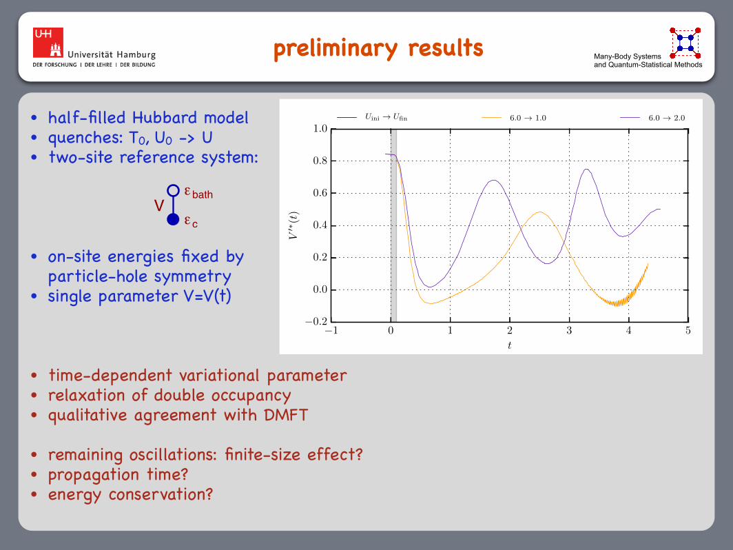
preliminary results Many-Body Systems and Quantum-Statistical Methods
Variants of DMFT FZ Jülich, 5.7.2007—————————————————————————————————————————————————————————–˛
˛
˛
˛
˛
˛
˛
˛
˛
˛
two-site DMFT
two-site impurity model:
εbath
εcV
3 (2) parameters to be determined
DMFT self-consistency condition: Gloc(ω) = G(ω)
3) high-frequency expansion of coherent part
z
0ω
DOS
G(coh)loc (ω) = G(coh)(ω)
z = 1/(1 − Σ′(0))
· · · +z3(M2 + (t0 − µ + a)2)
ω3+ · · · = · · · +
z2V 2 + z3(εc − µ + a)2)
ω3+ · · ·
second self-consistency conditions of two-site DMFT: M2 =1
L
X
k
ε(k)2 =X
j
t2ij
zM2 = V 2
. – p.8
• half-filled Hubbard model!• quenches: T0, U0 -> U!• two-site reference system:!
• on-site energies fixed by particle-hole symmetry!
• single parameter V=V(t)!
• time-dependent variational parameter!• relaxation of double occupancy!• qualitative agreement with DMFT!
• remaining oscillations: finite-size effect?!• propagation time?!• energy conservation?
1 0 1 2 3 4 5
t
0.00
0.05
0.10
0.15
0.20
0.25
d(t)
Uini ! Ufin 6.0 ! 1.0 6.0 ! 2.0
1 0 1 2 3 4 5
t
0.2
0.0
0.2
0.4
0.6
0.8
1.0
V0
(t)
Uini ! Ufin 6.0 ! 1.0 6.0 ! 2.0
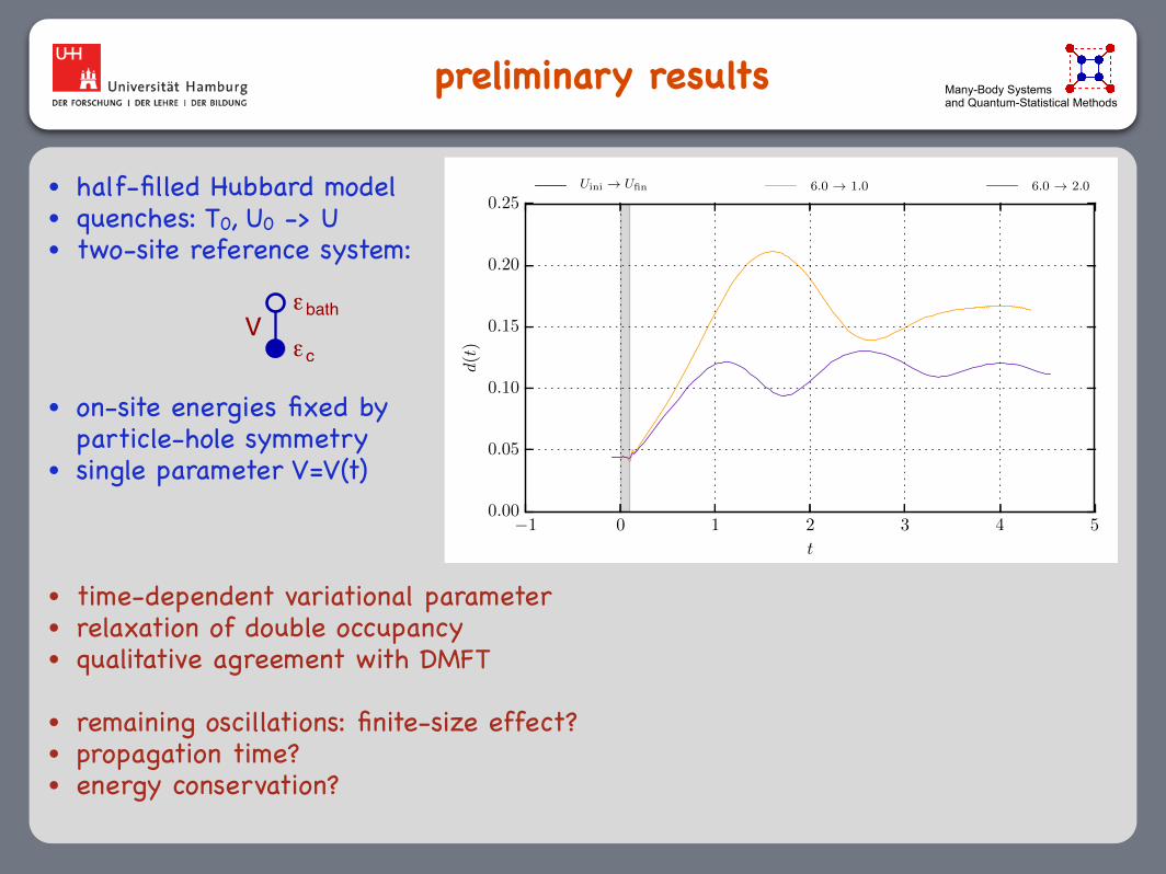
preliminary results Many-Body Systems and Quantum-Statistical Methods
Variants of DMFT FZ Jülich, 5.7.2007—————————————————————————————————————————————————————————–˛
˛
˛
˛
˛
˛
˛
˛
˛
˛
two-site DMFT
two-site impurity model:
εbath
εcV
3 (2) parameters to be determined
DMFT self-consistency condition: Gloc(ω) = G(ω)
3) high-frequency expansion of coherent part
z
0ω
DOS
G(coh)loc (ω) = G(coh)(ω)
z = 1/(1 − Σ′(0))
· · · +z3(M2 + (t0 − µ + a)2)
ω3+ · · · = · · · +
z2V 2 + z3(εc − µ + a)2)
ω3+ · · ·
second self-consistency conditions of two-site DMFT: M2 =1
L
X
k
ε(k)2 =X
j
t2ij
zM2 = V 2
. – p.8
• half-filled Hubbard model!• quenches: T0, U0 -> U!• two-site reference system:!
• on-site energies fixed by particle-hole symmetry!
• single parameter V=V(t)!
• time-dependent variational parameter!• relaxation of double occupancy!• qualitative agreement with DMFT!
• remaining oscillations: finite-size effect?!• propagation time?!• energy conservation?
1 0 1 2 3 4 5
t
0.00
0.05
0.10
0.15
0.20
0.25
d(t)
Uini ! Ufin 6.0 ! 1.0 6.0 ! 2.0
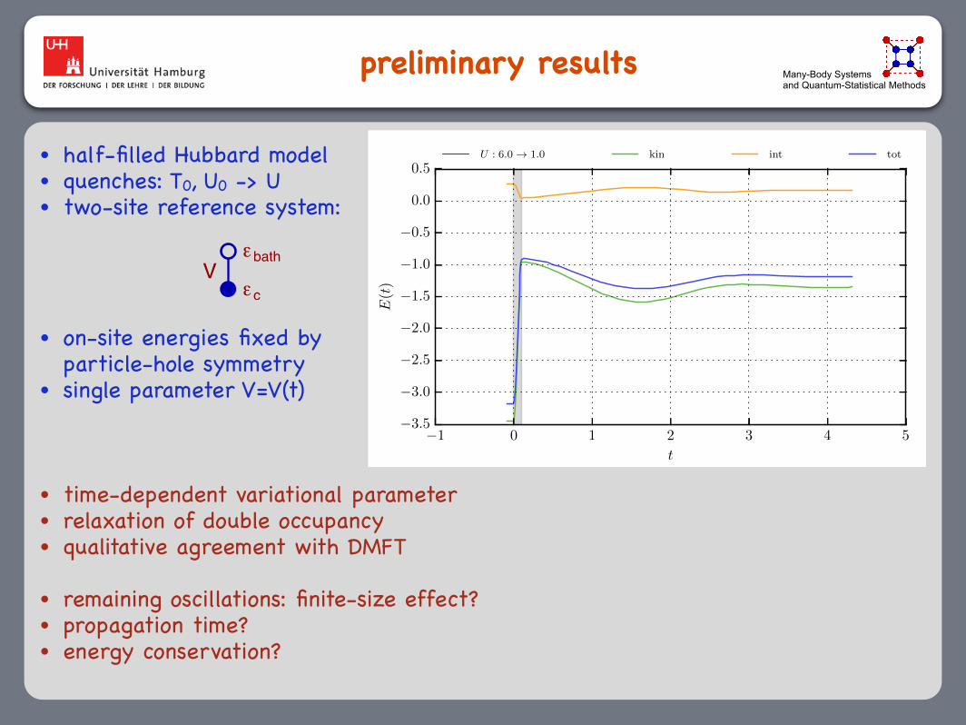
1 0 1 2 3 4 5
t
3.5
3.0
2.5
2.0
1.5
1.0
0.5
0.0
0.5
E(t
)
U : 6.0 ! 1.0 kin int tot

conserving approximations Many-Body Systems and Quantum-Statistical Methods
• for quench dynamics only!• time non-local variations required (needs continuum?)!• internal measure of approximation quality
(at short times: discrete level structure unimportant)!• enforce by constraint
“Phi-derivable approximations are conserving”
=
G
Baym, Kadanoff (1961)
equilibrium self-energy-functional theory Many-Body Systems
and Quantum-Statistical Methods
Kondo screening
Non-equilibrium self-energy-functional theory Ringberg Castle, 12.9.2011—————————————————————————————————————————————————————————–˛
˛
˛
˛
˛
˛
˛
˛
˛
˛
equilibrium self-energy-functional theory
time-independent Hamiltonian:H = HT + HU =
X
αβ
Tαβc†αcβ +1
2
X
αβγδ
Uαβδγc†αc†βcγcδ
Luttinger-Ward functional: = + + +ΦδΦU[G]
δG= ΣU[G]
Luttinger, Ward (1963)with
Gαβ(τ − τ ′) = −⟨cα(τ)c†β(τ ′)⟩ Matsubara Green’s function
⟨· · ·⟩ =1
Ztr (e−βH · · ·) grand-canonical expectation value
grand potential as a functional of the self-energy:
ΩT,U[Σ] = Tr ln1
G−1T,0 − Σ
+ FU[Σ]
Ω stationary at the physical self-energyδΩT,U[Σ]
δΣ= 0 for Σ = ΣT,U
Σ space
Ω
Ω = Ω[Σ]
δ Ω[Σ] = 0
. – p.3
HOFMANN, ECKSTEIN, ARRIGONI, AND POTTHOFF PHYSICAL REVIEW B 88, 165124 (2013)
The kinetic (and potential) energy Ekin(t) = ⟨HT ,0(t)⟩ andthe interaction energy Eint(t) = ⟨H0,U (t)⟩ of the system can bewritten as (see Refs. 46 and 47, for example)
Ekin(t) = −i tr[T (t)G(t,t+)], (72)
Eint(t) = − i
4tr[(! G + G !)(t,t+)]. (73)
The former directly follows from the definition of the Green’sfunction. For the latter, we made use of the equation of motionfor the Green’s function and Dyson’s equation. Note that wehave written G ≡ GT ,U and ! ≡ !T ,U for short. The totalenergy of the system is Etot(t) ≡ ⟨H (t)⟩ = Ekin(t) + Eint(t).In the following, we assume that the interaction parameters Uare time independent (see also discussion in Sec. XII C). Using∂tEtot(t) = ⟨∂tH (t)⟩, this immediately implies the followingenergy-balance relation:
∂Etot(t)∂t
=!
αβ
∂Tαβ(t)∂t
⟨c†α(t)cβ(t)⟩. (74)
Next, we express both the left-hand side and the right-handside of Eq. (74) in terms of ! and G. Using the equation ofmotion again, the time derivatives of Ekin(t) and Eint(t) can becomputed. From Eq. (72), we get
∂Ekin(t)∂t
=!
αβ
Tαβ([G,T ]βα(t,t+) + [G , !]βα(t,t+))
− i tr"
∂T (t)∂t
G(t,t+)#
=!
αβ
Tαβ[G , !]βα(t,t+) − i tr"
∂T (t)∂t
G(t,t+)#
.
(75)
Here, the first term in the first line vanishes due the cyclicproperty of the trace. Exploiting once more the equation ofmotion and the complex-conjugated equation, we find
∂Ekin(t1)∂t1
= i!
α1
$d2
%"∂
∂t1G(1,2)
#$(2,1+)
+$(1,2)∂
∂t1G(2,1+)
&
− i tr"
∂T (t1)∂t1
G(t1,t+1 )#
. (76)
Note that the last summand just equals the right-hand side ofEq. (74). This equation can easily be combined with the timederivative of the interaction energy [Eq. (73)]. After applyingthe product rule, the energy-balance relation [Eq. (74)] is
expressed as47
−34
!
α1
$d2
∂
∂t1[$(1,2)G(2,1+) + G(1,2)$(2,1+)]
+!
α1
$d2
"∂$(1,2)
∂t1G(2,1+) + G(1,2)
∂$(2,1+)∂t1
#
= 0. (77)
An approximation constructed within the SFT will respectenergy balance if Eq. (77) holds but with ! replaced by !λ′
opt,U
and with G replaced by GSFT. Thus, the goal is to find a classof transformations of the one-particle parameters such thattheir corresponding first-order variations around the stationarypoint generate the above equation as the SFT Euler equation.In principle, this can be achieved with
λ′(z) '→ λ′(z) = i(1 − θ−1/2)∂z + i
4θ−3/2θ + θ1/2λ′(θ ),
(78)
where θ (z) is an arbitrary real function on the contour with∂zθ (z) = 0 which describes a transformation of the time scale.Note that due to the term ∝ ∂z the action of λ
′(z) is nonlocalin time. This is a severe complication if λ
′(z) should representparameters of an actual impurity Hamiltonian, as discussedin Sec. XII C. It is nevertheless illustrative to see how energyconservation can be derived if the self-energy functional isstationary under the variations defined by Eq. (78).
The time-dependent transformation of the one-particleparameters induces a corresponding transformation of theexact Green’s function G′ ≡ Gλ′,U and of the exact self-energy!′ ≡ !λ′,U of the reference system. For G′, we have
G′(z1,z2) '→ G′(z1,z2) = θ1/41 G′(θ1,θ2)θ1/4
2 , (79)
where the shorthand notation θ1 = θ (z1) and θ1 = ∂z1θ (z1),etc., is used. Via the skeleton-diagram expansion !′ ='!U [G′], this induces the following transformation of theself-energy:
!′(z1,z2) '→ !′(z1,z2) = θ
3/41 !′(θ1,θ2)θ3/4
2 . (80)
Namely, any internal vertex at time zi connects to fourpropagators and thereby collects a factor θi by which theimplicit zi integration can be transformed into a θi integration.The factors θ
3/41 and θ
3/42 in Eq. (80) result from the three
incoming and outgoing propagators at the two “external”vertices. Now, Eq. (79) is verified by showing that the assertedexpression for the transformed Green’s function G′(z1,z2)together with Eq. (80) satisfies the equation of motion fortransformed one-particle parameters [Eq. (78)]. A proof forthis can be found in Appendix E.
The first-order variations of !′ induced by this transforma-tion, δ!′ = δ!′(θ1,θ2)/δθ |θ=t δθ , are given by
δ$′(2,1) =$
Cdz
%34$′(2,1)
"∂
∂z2δ(z2 − z)
#+ 3
4$′(2,1)
"∂
∂z1δ(z1 − z)
#
+"
∂
∂z2$′(2,1)
#δ(z2 − z) +
"∂
∂z1$′(2,1)
#δ(z1 − z)
&δθ (t). (81)
165124-12
Non-equilibrium self-energy-functional theory Ringberg Castle, 12.9.2011—————————————————————————————————————————————————————————–˛
˛
˛
˛
˛
˛
˛
˛
˛
˛
NON-EQUILIBRIUM self-energy-functional theory
TIME-DEPENDENT Hamiltonian:Ht = HT(t) + HU(t) =
X
αβ
Tαβ(t)c†αcβ +1
2
X
αβγδ
Uαβδγ(t)c†αc†βcγcδ
Luttinger-Ward functional: = + + +ΦδΦU[G]
δG= ΣU[G]
withGαα′ (t, t′) = −i⟨cα(t)c†
α′ (t′)⟩ CONTOUR-ORDERED Green’s function
⟨· · ·⟩ =1
Ztr (e−βHt0 · · ·) grand-canonical expectation value
INITIAL-STATE grand potential:
ΩT,U[Σ] = Tr ln1
G−1T,0 − Σ
+ FU[Σ]
Ω stationary at the physical self-energyδΩT,U[Σ]
δΣ= 0 for Σ = ΣT,U
Σ space
Ω
Ω = Ω[Σ]
δ Ω[Σ] = 0
. – p.7
non-equilibrium self-energy-functional theory
Hofmann, Eckstein, Arrigoni, Potthoff, arXiv:1306.6340
T0(z) ! ei(z)T0(z)ei "0(z) ! "0(z) @z
variations of T’ comprise gauge transformations
stationary point: proliferation of conservation laws (U(1), SU(2), ...)
reference system (exact)
original system (with SFT Green’s function and self-energy)
SFT generates non-perturbative conserving approximations !
total!energy !conserv.!
conclusions and outlook Many-Body Systems and Quantum-Statistical Methods
• non-equilibrium cluster-perturbation theory: diagrammatic reformulation possible non-uniqueness can be exploited to set up a variational theory!
• non-equilibrium self-energy-functional theory: based on dynamical variational principleapproximations generated by restricting the domain of the self-energy functional!
• relation to non-equilibrium dynamical mean-field theory:NE-DMFT is re-derived (the same for C-DMFT, DCA, PC-DMDT)more simple approximations can be constructed: DIA/VCA, building on Lanczos/Krylov techniques!
• open methodical problems: more systematic studies neededcode optimization to access much longer time scales convergence as a function of the number of bath degrees of freedom conservation of total energy: constrained variation?!
• SFT - new directions: reference systems with different interactions / fully universal functionals…!


![)UHH 3ULQWDEOH 6FKRRO /XQFK -RNHV · )uhh 3ulqwdeoh 6fkrro /xqfk -rnhv 7kh\ duh dozd\v vwxiihg 7r jr zlwk wkh mhoo\ilvk %rrnzrupv %\ vfkrro ex]] :ulwh rq 3rvw 2iilfh %hfdxvh shsshu](https://img.pdfslide.us/doc/110x75/5e43b42c38bf5662ff74e651/uhh-3ulqwdeoh-6fkrro-xqfk-rnhv-uhh-3ulqwdeoh-6fkrro-xqfk-rnhv-7kh-duh-dozdv.jpg)


![s } o X ñ ñ / µ ï D Z î ì í õ 7KH %UHH]Hparkpointcommunityclub.org/wp-content/uploads/2009/04/March-2019... · fdelqhw rog %uhh]hv iurp zklfk uhyhdohg wkdw zh duh wdonlqj](https://img.pdfslide.us/doc/110x75/5e7ba0dd6b4fba318a208588/s-o-x-d-z-7kh-uhhhpa-fdelqhw-rog-uhhhv-iurp-zklfk.jpg)


![6HD%UHH]H - Pronto Marketing...0DLQ'HFN %HR9LVLRQ 79 +7 VSHDNHUV.DUWKUHLQ6DWUHFHLYHU8)' 2ZQHU V6XLWH %HR9LVLRQ 79 /RZHUGHFN +7 VSHDNHUV.DUWKUHLQ6DWUHFHLYHU8)' *XHVW&DELQV %HR9LVLRQ](https://img.pdfslide.us/doc/110x75/5f601c2a4d75f52f7e61105e/6hduhhh-pronto-marketing-0dlqhfn-hr9lvlrq-79-7-vshdnhuvduwkuhlq6dwuhfhlyhu8.jpg)

![7KH %UHH]H - Park Point Community Club](https://img.pdfslide.us/doc/110x75/627c159906062911b020ae87/7kh-uhhh-park-point-community-club.jpg)