Embed Size (px)
Citation preview

OSD7, 335–360, 2010
Trends in coastalupwelling intensity
N. Narayan et al.
Title Page
Abstract Introduction
Conclusions References
Tables Figures
J I
J I
Back Close
Full Screen / Esc
Printer-friendly Version
Interactive Discussion
Ocean Sci. Discuss., 7, 335–360, 2010www.ocean-sci-discuss.net/7/335/2010/© Author(s) 2010. This work is distributed underthe Creative Commons Attribution 3.0 License.
Ocean ScienceDiscussions
This discussion paper is/has been under review for the journal Ocean Science (OS).Please refer to the corresponding final paper in OS if available.
Trends in coastal upwelling intensityduring the late 20th centuryN. Narayan, A. Paul, S. Mulitza, and M. Schulz
MARUM – Center for Marine Environmental Sciences and Faculty of Geosciences,University of Bremen, Germany
Received: 21 January 2010 – Accepted: 8 February 2010 – Published: 19 February 2010
Correspondence to: N. Narayan ([email protected])
Published by Copernicus Publications on behalf of the European Geosciences Union.
335

OSD7, 335–360, 2010
Trends in coastalupwelling intensity
N. Narayan et al.
Title Page
Abstract Introduction
Conclusions References
Tables Figures
J I
J I
Back Close
Full Screen / Esc
Printer-friendly Version
Interactive Discussion
Abstract
This study presents linear trends of coastal upwelling intensity in the later part of the20th century (1960–2001) employing various indices of upwelling, derived from merid-ional wind stress and sea surface temperature. The analysis was conducted in the fourmajor coastal upwelling regions in the world, which are off North-West Africa, Luderitz,5
California and Peru respectively. The trends in meridional wind stress showed a steadyincrease of intensity from 1960–2001, which was also reflected in the SST index cal-culated for the same time period. The steady cooling observed in the instrumentalrecords of SST off California substantiated this observation further. Correlation analy-sis showed that basin-scale oscillations like the Atlantic Multidecadal Oscillation (AMO)10
and the Pacific Decadal Oscillation (PDO) could not be directly linked to the observedincrease of upwelling intensity off NW Africa and California respectively. The rela-tionship of the North Atlantic Oscillation (NAO) with coastal upwelling off NW Africaturned out to be ambiguous due to a negative correlation between the NAO index andthe meridional wind stress and a lack of correlation with the SST index. Our results15
give additional support to the hypothesis that the coastal upwelling intensity increasesglobally because of raising greenhouse gas concentrations in the atmosphere and anassociated increase of the land-sea pressure gradient and meridional wind stress.
1 Introduction
Coastal upwelling systems are characterized by seasonally low sea-surface tempera-20
ture (SST). Coastal upwelling results from the response of the coastal ocean to along-shore winds, leading to the production of a relatively intense current with a smalloffshore and a large alongshore component (e.g. Pedlosky, 1978). This causes thepumping of cooler and nutrient-rich water from the subsurface (from 50–150 m approx-imately) to the ocean surface.25
Due to the enhanced primary production, these regions are economically important
336

OSD7, 335–360, 2010
Trends in coastalupwelling intensity
N. Narayan et al.
Title Page
Abstract Introduction
Conclusions References
Tables Figures
J I
J I
Back Close
Full Screen / Esc
Printer-friendly Version
Interactive Discussion
accounting to nearly 20% of the global fish catch, even though the area constituted bythe upwelling regions are less than 1% of the global ocean (Pauly and Christensen,1994). They also play an important role in the air sea exchange of CO2. Moreover,coastal upwelling has also a profound effect on local climate.
Based on pre-1985 data, Bakun (1990) observes an increase in coastal upwelling5
at a global scale. He hypothesizes that this increase is due to global warming. Theunderlying mechanisms involve an intensification of the land-sea pressure gradient dueto the differential heating, which in turn cause a strengthening of upwelling-favorablewinds.
In support of the “Bakun hypotheis”, a significant cooling of surface waters in the10
coastal upwelling area off Cape Ghir (North West Africa near 30.5◦ N) during the laterpart of the 20th century has been reconstruced by McGregor et al. (2007). However,Lemos and Pires (2004) find a decrease in coastal upwelling intensity off the coast ofPortugal in the later part of the 20th century. Furthermore, Dunbar (1983) suggestsa decrease of upwelling between 1850 and the present. While taking into account a15
longer timescale of 3000 years, Julliet-Leclerc and Schrader (1987) also argue that thecoastal upwelling in the Gulf of California is weaker today than 1500 to 2000 yearsbefore present. These contrasting results prompted us to study the change of coastalupwelling intensity during the 20th century in further detail.
In this study we test the Bakun hypothesis on a global scale by exploiting available20
datasets covering a longer time period and extending to the present day. To this end,we compared the linear trends of coastal upwelling intensity, which we derived frommeridional wind stress and SST, in the four major upwelling regions of the world. Wealso tested if basin-scale climate oscillations exert a primary control over the intensityof coastal upwelling. The analysis revealed contrasting trends which suggested large25
discrepancies between the wind-stress datasets. The datasets that we regard as morereliable support an increase of coastal upwelling intensity over the later part of 20thcentury, which is consistent with the observation by Bakun (1990).
337

OSD7, 335–360, 2010
Trends in coastalupwelling intensity
N. Narayan et al.
Title Page
Abstract Introduction
Conclusions References
Tables Figures
J I
J I
Back Close
Full Screen / Esc
Printer-friendly Version
Interactive Discussion
2 Data and methods
Our analysis focuses on the coastal-upwelling areas off North West Africa (near30.5◦ N), California (near 39◦ N), Luderitz (near 27.5◦ S) and Peru (near 12.5◦ S). Due tothe lack of long-term and regional-scale measurements of vertical velocities, we usedwind speed and SST as an indirect measure for assessing upwelling strength. We5
employed the meridional wind speed data of the Comprehensive Ocean AtmosphereDataset (COADS; Slutz et al., 1985), the National Center for Environmental Predic-tion NCEP/NCAR reanalysis (Kalnay et al., 1996) and the ERA 40 reanalysis (Uppalaet al., 2005) from the European Centre for Medium Range Weather Forecast. TheCOADS dataset has a spatial resolution of 1◦×1◦, while the NCEP/NCAR reanalysis10
and the ERA 40 reanalysis both have a spatial resolution of 2.5◦×2.5◦. For obtainingthe timeseries a small region (3◦ in the cross-shore direction and 5◦ in the alongshoredirection) was defined in each of the coastal upwelling areas and the meridional windstress was area-averaged. The data over land areas were masked out. All data wereobtained at a monthly resolution and averaged over time to produce annual data. The15
time period covered by the wind data is from 1960 to 2001. An increase in equatorwardmeridional wind stress was taken to indicate an increase in coastal upwelling. Windstress was calculated from wind speed using a constant drag coefficient of 1.2. TheCOADS wind stress at a monthly resolution was used for calculating Pearson’s corre-lation coefficient and the cross-correlation coefficients with climatic indices indicative of20
the Atlantic Multidecadal Oscillation (AMO), the North Atlantic Oscillation (NAO), andthe Pacific Decadal Oscillation (PDO).
We also used the SST data from the Hadley Centre (HadISST; Rayner et al., 2003)which is a monthly dataset with a spatial resolution of 1◦×1◦ that covers the time pe-riod 1870–2006. The monthly data was averaged over time to produce annual data25
and was used to calculate an index of coastal upwelling, which is defined as the dif-ference of SST from an offshore location to a near shore location at the same latitude(Nykjaer and Van Camp, 1994). For this purpose a series of locations was determined
338

OSD7, 335–360, 2010
Trends in coastalupwelling intensity
N. Narayan et al.
Title Page
Abstract Introduction
Conclusions References
Tables Figures
J I
J I
Back Close
Full Screen / Esc
Printer-friendly Version
Interactive Discussion
on the coast separated by 1◦in the meridional direction. A location 5◦offshore from thecoastal point was taken at the same latitude as the offshore data point (Fig. 1). TheSST index was calculated by subtracting the SST at the coastal point from the SST atthe offshore location. Through this method five different time series were obtained foreach upwelling region. The average of these time series was then taken as the up-5
welling index. An increase of this index is taken to indicate an increase of the upwellingintensity. An SST index with monthly temporal resolution was also calculated by theabove method for the correlation and cross-correlation analysis with various climaticindices.
In addition, the instrumental SST dataset provided by the California Cooperative10
Fisheries Investigation (CALCOFI; Bograd et al., 2003) was used in the California up-welling region to also calculate an upwelling index. The SST data east of CALCOFIstation number 52 was taken as coastal data and the SST data between west of CAL-COFI station number 80 was considered offshore data (Fig. 2). The data points in theSea of Cortez were excluded. An upwelling index time series was produced by sub-15
tracting the coastal SST from the offshore SST. A time series of temperature of the top100 m of the water column in the coastal area (east of CALCOFI station number 52)was also taken. Though the CALCOFI data extends from 1949–2006, there are gaps inthe time series when the CALCOFI cruises were not frequent, especially between 1970and 1980. However, overall trends in the data could be used as shown in the study by20
Roemmich (1992). The resulting time series had a temporal resolution of three months(starting in January) and was area-averaged.
The following climatic indices at monthly resolution were used in the study:
1. The Atlantic Multi-decadal Oscillation Index (AMOI; Enfield et al., 2001) calcu-lated from the SST data of Kaplan et al. (1998) as the de-trended area-weighted25
average over the North Atlantic (0◦–70◦ N).
2. The North Atlantic Oscillation Index (NAOI; Barnston and Livezey, 1987), whichis the normalised pressure difference between the Azores and Iceland averaged
339

OSD7, 335–360, 2010
Trends in coastalupwelling intensity
N. Narayan et al.
Title Page
Abstract Introduction
Conclusions References
Tables Figures
J I
J I
Back Close
Full Screen / Esc
Printer-friendly Version
Interactive Discussion
over the months of December, January and February.
3. The Pacific Decadal Oscillation Index (PDOI; Mantua et al., 1997) derived asthe leading principal component of monthly SST anomalies in the North PacificOcean, poleward of 20◦ N with monthly means removed.
4. The Multivariate El Nino Southern Oscillation Index (MEI; Wolter and Timlin, 1993)5
based on the sea-level pressure, zonal and meridional components of the surfacewind, sea surface temperature, surface air temperature and the total cloudinessfraction of the sky.
The time series of meridional wind stress and SST index were low-pass filtered us-ing a Butterworth filter with a cutoff period of 8 years and order 12. This was done to10
reduce the effect of interannual variability on the long term trend. Due to the presenceof gaps in the CALCOFI dataset the high pass filtering could not be performed on itand the raw data was used for the analysis. Linear trends in time series were esti-mated using the method of least squares. The statistical significance of the trends wasestimated using a Student’s t-test with the null hypothesis of a zero slope of the trend15
line at a significance level of 0.05. In order to account for the autocorrelation in timeseries, an effective sample size was used (Dawdy and Matalas, 1964). The correlationbetween time series along with the bootstrap confidence interval was estimated takinginto account the serial dependence in the timeseries (Mudelsee, 2003). The cross-correlation function was calculated using the algorithm described by Orfanidis (1996).20
Linear trends were removed from the datasets before estimating the cross-correlationfunction.
3 Results
The COADS wind stress reveals significant increasing trends in all coastal upwellingregions (Fig. 3, Table 1). In contrast the NCEP/NCAR wind stress (Fig. 4, Table 1)25
340

OSD7, 335–360, 2010
Trends in coastalupwelling intensity
N. Narayan et al.
Title Page
Abstract Introduction
Conclusions References
Tables Figures
J I
J I
Back Close
Full Screen / Esc
Printer-friendly Version
Interactive Discussion
indicated a significant decrease in upwelling off NW Africa, whereas an increasing trendwas observed in Luderitz. The trends for California and Peruvian upwelling regionswere statistically insignificant.
The ERA40 (Fig. 5, Table 1) dataset showed an increasing trend in the NW Africanand Peru upwelling regions and a decreasing trend in the California upwelling region.5
In the Luderitz upwelling region the trend observed is insignificant.As an additional proxy for upwelling intensity, the SST index was calculated for the
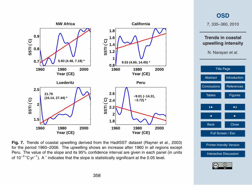
period between 1870 and 2006 and analysed for trends (Fig. 6, Table 1). It revealedsignificantly decreasing trends off NW Africa, Luderitz and Peru. In contrast, trends inthe more recent part of the time series (from 1960 onwards) suggested an increase in10
upwelling in all regions except off Peru (Fig. 7, Table 1).For the California system, this result is also supported by the SST index derived
from the CALCOFI dataset California (Fig. 8a). The coastal SST indicated a significantcooling trend throughout the sampling period (Fig. 8b). The time series produced byaveraging the temperature of the top 100 m of the water column in the California coastal15
region also showed a significant cooling (Fig. 8c). Both findings confirmed the resultsobtained by analysing the wind and SST data from the global datasets.
4 Discussion
On one hand, the results from analysing trends in the COADS wind stress are consis-tent with the hypothesis by Bakun (1990), later taken up by McGregor et al. (2007) for20
NW Africa, which proposes a general increase in coastal upwelling in the later part ofthe 20th century due to global warming. On the other hand, trends obtained from theNCEP/NCAR and ERA40 wind stress for the areas off NW Africa as well as the studyby Lemos and Pires (2004), which argues that the upwelling intensity has decreasedover the last century at the coast of Portugal, suggest that coastal upwelling intensity25
is increasing in some upwelling regions and decreasing in others.At first sight the lack of significant trends in the Luderitz (ERA40 dataset) and Califor-
341

OSD7, 335–360, 2010
Trends in coastalupwelling intensity
N. Narayan et al.
Title Page
Abstract Introduction
Conclusions References
Tables Figures
J I
J I
Back Close
Full Screen / Esc
Printer-friendly Version
Interactive Discussion
nia (NCEP/NCAR dataset) and the existence of significant decreasing trends revealedby the NCEP/NCAR dataset for the NW African and Peruvian upwelling regions in-deed seem to contradict the global nature of increasing coastal upwelling intensity asproposed by Bakun (1990). However, Smith et al. (2001) argue that the NCEP/NCARreanalysis dataset underestimates the strength of wind globally. They also suggest5
that the surface pressure is significantly weaker in the tropics, which leads to an un-derestimation of the strength of subtropical highs and the wind strength, specifically inthe subtropics. Moreover, the comparison of NCEP/NCAR winds with COADS windsby Wu and Xie (2003) revealed that the COADS inter-decadal wind changes are moreconsistent with independent observations. Based on these findings we assume that10
the trends observed in the COADS dataset are likely to be more reliable.The trend observed in the SST index derived from the HadISST in the later part
of the 20th century (1960–2006) also showed a significant increase of upwelling inall regions except Peru and is thus consistent with the wind stress derived from theCOADS data. It should be noted that the trend obtained from the HadISST data after15
1960 off Peru demonstrates a significant decrease of upwelling even when upwellingfavourable winds derived from the COADS dataset and the ERA 40 dataset show asignificant increase. A comparision of the filtered and unfiltered SST index for thePeruvian upwelling region with the MEI (Fig. 9) reveals that the time interval 1962–1975 was predominantly in the cooler than normal (La Nina) phase, whereas the MEI20
indicates predominantly warmer than normal conditions after 1975. The presence of arelatively cool phase in the earlier part of the time series and a relatively warm phasein the later part effectively led to an apparent decrease of coastal upwelling. This isreflected even in the filtered time series where the peaks associated with the El Nino/LaNina are removed.25
The trends obtained from the CALCOFI SST index and coastal temperatures indicatea significant cooling trend. This further substantiates the result obtained from COADSwind stress and the HadISST index. It is also consistent with the increase in net primaryproduction inferred from satellite observations from 1997 to 2007 (Kahru et al., 2009).
342

OSD7, 335–360, 2010
Trends in coastalupwelling intensity
N. Narayan et al.
Title Page
Abstract Introduction
Conclusions References
Tables Figures
J I
J I
Back Close
Full Screen / Esc
Printer-friendly Version
Interactive Discussion
The coastal upwelling areas especially off NW Africa and California are subject tobasin-scale climate oscillations like the Atlantic Mutidecadal Oscillation (AMO), theNorth Atlantic Oscillation (NAO) and the Pacific Decadal Oscillation (PDO). So thetrends observed in the upwelling intensity could be affected by these basin-scale oscil-lations. In the following we want to exclude the possibility that these oscillations exert5
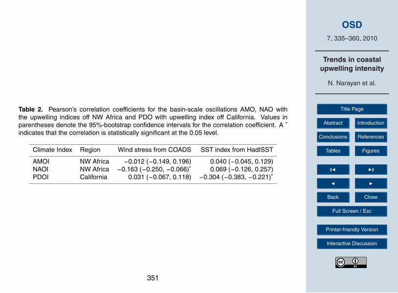
a primary control over the intensity of coastal upwelling.With regard to the possible control of the upwelling intensity by basin-scale climate
oscillation, Pearson’s correlation coefficient (see Table 2) showed that the correlationbetween the upwelling indices off NW Africa and the AMOI is insignificant. Further-more, the NAOI shows a significant negative correlation with the meridional wind stress10
off NW Africa, but the correlation with the SST index is insignificant. Finally, the corre-lation coefficient between the PDOI and the SST index of coastal upwelling indices offCalifornia showed a weak but significant correlation but the correlation with alongshorewind stress was found to be insignificant.
Cross-correlation analyses (not shown) between the upwelling indices off NW Africa15
and the AMOI revealed the lack of correlation at all lags. The cross-correlation betweenNAOI and upwelling indices off NW Africa also showed no significant correlation at anylag. In the North Pacific, the PDOI and upwelling indices off California also failed toshow any substantial cross-correlation at any lag. Francis et al. (1998) observed thatduring the positive phase of the PDO, salmon fish catches have been significantly re-20
duced in the California Current System and the associated upwelling region. Since thePDO reversed its direction in 1977 to its positive phase and remained in it until late1990’s, the majority of the data used in our study originate from a positive phase of thePDO. Correlation and cross-correlation analyses were done to check the influence ofthe PDO on the coastal upwelling off California. A weak but significant negative corre-25
lation −0.304 (−0.383, −0.221) was observed with the SST index, that is, weaker up-welling during a positive phase of the PDO. However, the correlation between the PDOand wind stress was insignificant. According to Roemmich and McGowan (1995), thewarming associated with the shift towards the positive phase of the PDO increases the
343

OSD7, 335–360, 2010
Trends in coastalupwelling intensity
N. Narayan et al.
Title Page
Abstract Introduction
Conclusions References
Tables Figures
J I
J I
Back Close
Full Screen / Esc
Printer-friendly Version
Interactive Discussion
stratification, which in turn would result in the reduced displacement of the thermoclineand increase the temperature of the upwelled water. Therefore the PDO may exert acertain amount of control on SST in the California region, but not neccessarily on thewind stress. In line with the Bakun hypothesis, the increasing trend in wind stress couldbe due to global warming and, hence, exert an independent control on SST.5
The North Atlantic Oscillation could influence the coastal upwelling intensity off theNW-African region because of its influence on the Azores high (Knippertz et al., 2003).The NAO also has a very important role in the long-term variability of the wind in theNorth Atlantic (Santos et al., 2005). The NAO was in the negative phase at the startof the data used in our analysis, changing to its positive phase during early 1980’s.10
Since two different phases of the NAO were present in the period of our study, we mayexpect an influence of the NAO on the trend of coastal upwelling. Hence a correlationanalysis was conducted between the NAO index and the upwelling indices off NWAfrica to disentangle any plausible relation between the two (Table 2). The correlationanalysis revealed a significant negative correlation with the alongshore wind stress but15
an insignificant correlation with the SST index. The cross-correlation analysis also didnot reveal any relation between the upwelling index and NAO. The lack of correlationbetween the SST index and NAO is quite ambiguous considering a significant negativecorrelation with the alongshore wind stress. Hence the influence of the NAO on theincreasing trend of coastal upwelling could not be substantiated.20
Similarly, the AMO is also a main factor in the long term evolution of wind and SSTin the North Atlantic. Knight et al. (2006) argue that during the warm phase of AMOthere are consistent changes of the trade winds over the Sahel region and also anorthward displacement of the mean Inter Tropical Convergence Zone. The NorthAtlantic experienced a change from a warm phase to a cold phase in the mid 1960’s,25
and the AMO again shifted to a warm phase during the mid 1990’s. Accordingly changein the trade-wind patterns associated with the changing phase of the AMO could be aconsiderable factor in determining the long-term trend of coastal upwelling intensity.However, the correlation between the AMO index and coastal upwelling indices were
344

OSD7, 335–360, 2010
Trends in coastalupwelling intensity
N. Narayan et al.
Title Page
Abstract Introduction
Conclusions References
Tables Figures
J I
J I
Back Close
Full Screen / Esc
Printer-friendly Version
Interactive Discussion
statistically insignificant which allows us to disregard any primary control of the AMOover the intensity of coastal upwelling off NW Africa.
The major physical factor which controls coastal upwelling intensity along the easternboundaries of the oceans is the equator-ward alongshore wind stress component. Thehypothesis proposed by Bakun (1990) puts forth a mechanism by which the wind stress5
that favours the upwelling increases due to the greenhouse gas-induced warming andsubsequent changes in the land-sea pressure gradient. This mechanism may alsoserve as an explanation for the trends in the COADS wind stress data and the SSTindices derived from the HadISST and the CALCOFI SST datasets.
Stratification is another important factor in determining the depth from which the wa-10
ter upwells, which in turn affects the coastal SST and nutrient concentration. Upwellingoccurring due to divergence in the alongshore current and topographic steering is an-other possible process by which the rate of upwelling can be altered over time. But theeffect of these processes on long-term variability in a coastal upwelling system is notwell documented.15
5 Conclusions
From the analysis of trends in wind stress obtained from the COADS, NCEP/NCAR andERA 40 datasets, we found that there were large discrepancies between the datasets.Based on the comparisons done in previous studies, we consider the trends obtainedfrom the COADS dataset to be most reliable. These trends indicate an increase of20
coastal upwelling in all major upwelling regions.The SST index obtained from the HadISST data suggests a decrease of coastal
upwelling after 1870. However, after 1960 the same SST index also shows a significantincrease of coastal upwelling in all regions except for Peru. Additionally, the CALCOFIdataset presents strong evidence for the intensification of upwelling in the California25
upwelling region.Our study revealed that AMO does not directly interact with upwelling off NW Africa.
345
OSD7, 335–360, 2010
Trends in coastalupwelling intensity
N. Narayan et al.
Title Page
Abstract Introduction
Conclusions References
Tables Figures
J I
J I
Back Close
Full Screen / Esc
Printer-friendly Version
Interactive Discussion
The influence of NAO with upwelling off NW Africa seems to be quite ambiguous, as anegative correlation between the NAOI and meridional wind stress is observed, but acomplete lack of correlation with the SST index was found. In the Pacific the PDOI alsoshows a weak correlation with upwelling off California, indicating a lack of any directinteraction.5
In summary, the hypothesis proposed by Bakun (1990) and later taken up by McGre-gor et al. (2007), which states there is an intensification of coastal upwelling in relationto global climate change, gains additional support by our analysis of the COADS windstress data, the SST index derived from the HadISST data (after 1960) and the SSTindex derived from the CALCOFI data set. The lack of correlation between the basin-10
scale oscillations like the AMO, the NAO and the PDO also rules out an alterationof upwelling intensity other than due to enhanced upwelling-favourable winds by themechanism proposed by Bakun (1990).
Acknowledgements. The study is funded through DFG-Research Center/Excellence Cluster“The Ocean in the Earth System” and the “Bremen International Graduate School for Marine15
Sciences (GLOMAR)”.
References
Bakun, A.: Global climate change and intensification of coastal ocean upwelling, Science, 247,198–201, 1990. 337, 341, 342, 345, 346
Barnston, A. G. and Livezey, R. E.: Classification, seasonality and persistence of low-20
frequency atmospheric circulation patterns, Mon. Weather Rev., 115, 1083–1126, onlineavailable at: http://www.cpc.noaa.gov/products/precip/CWlink/pna/norm.nao.monthly.b5001.current.ascii, 1987. 339
Bograd, S. J., Checkley Jr., D. A, and Wooster, W. S.: CalCOFI: a half century of physical,chemical, and biological research in the California Current System, Deep Sea Res. II, 50,25
14–16, 2003. 339, 353, 359Borges, M. F., Santos, A. M. P., Crato, N., Mendes, H., and Mota, B., Sardine regime shifts
346

OSD7, 335–360, 2010
Trends in coastalupwelling intensity
N. Narayan et al.
Title Page
Abstract Introduction
Conclusions References
Tables Figures
J I
J I
Back Close
Full Screen / Esc
Printer-friendly Version
Interactive Discussion
off Portugal: a time series analysis of catches and wind conditions, Scientia Marina, 67,235–244, 2003.
Dawdy, D. R. and Matalas, N. C.: Statistical and probability analysis of hydrologic data, Part 3,analysis of variance, covariance, and time series, Handbook of Applied Hydrology Ed. VenTe Chow, McGraw-Hill, New York, 1964. 3405
Dunbar, R. B.: Stable isotope record of upwelling and climate from Santa Barbara Basin, Cal-ifornia Coastal Upwelling, Its Sediment Rec., edited by: Thiedel, J. and Suess, E., Plenum,New York, 217–246, 1983. 337
Ekman, W. K.: On the influence of earth’s rotation on ocean currents, Arkiv for Matematik,Astronomi och Fysik, 2, 1–53, 1905.10
Enfield, D. B., Mestas-Nunez, A. M., and Trimble, P. J.: The Atlantic Multidecadal Oscillation andits relationship to rainfall and river flows in the continental US, Geophys. Res. Lett., 28, 2077–2080, online available at: http://www.cdc.noaa.gov/data/correlation/amon.sm.data, 2001.339
Francis, C. R., Hare, S. R., Hollowed, A. B., and Wooster, W. S.: Effects of interdecadal climate15
variability on the oceanic ecosystem of the NE Pacific, Fish. Oceanogr., 7, 1–21, 1998. 343Hagen, E.: Mesoscale upwelling variations off the West African coast, Coastal Upwelling,
edited by: Richards, F. A., American Geophysical Union, 72–78, 1981.Jin, F. F.: An equatorial ocean recharge paradigm for ENSO. Part I: conceptual model, J. Atmos.
Sci., 54, 811–829, 1997.20
Juillet-Leclerc A. and Schrader H.: Variations in upwelling intensity recorded in varved sedimentfrom the Gulf of California during the past 3000 years, Nature, 329, 146–149, 1987. 337
Kahru, M., Kudela, R., Manzano-Sarabia, M., and Mitchell, B. G.: Trends in primary produc-tion in the California Current detected with satellite data, J. Geophys. Res., 114, C02004,doi:10.1029/2008JC004979, 2009. 34225
Kalnay, E., Kanamitsu, M., Kistler, R., Collins, W., Deaven, D., Gandin, L., Iredell, M., Saha,S., White, G., Woollen, J., Zhu, Y., Chelliah, M., Ebisuzaki, W., Higgins, W., Janowiak, J.,Mo, K. C., Ropelewski, C., Wang, J., Leetmaa, A., Reynolds, R., Jenne, R., and Joseph, D.:The NCEP/NCAR 40-Year Reanalysis Project, B. Am. Meteorol. Soc., 77(3), 437–471, 1996.338, 35530
Kaplan, A., Cane, M., Kushnir, Y., Clement, A., Blumenthal, M., and Rajagopalan, B.: Analysesof global sea surface temperature 1856–1991, J. Geophys. Res., 103, 18567–18589, 1998.339
347

OSD7, 335–360, 2010
Trends in coastalupwelling intensity
N. Narayan et al.
Title Page
Abstract Introduction
Conclusions References
Tables Figures
J I
J I
Back Close
Full Screen / Esc
Printer-friendly Version
Interactive Discussion
Knight, J. R., Folland, C. K., and Scaife, A. A.: Climate impacts of the Atlantic MultidecadalOscillation, Geophys. Res. Lett., 33, L17706, doi:10.1029/2006GL026242, 2006. 344
Knippertz, P., Christoph, M., and Speth, P.: Long-term precipitation variability in Morocco andthe link to large-scale circulation in recent and future climates, Meteorol. Atmos. Phys., 83,67–88, 2003. 3445
Lemos, R. T. and Pires, H. O.: The upwelling regime off the West Portuguese Coast, 1941–2000, Int. J. Climatol., 24, 511–524, 2004. 337, 341
Mantua, N. J., Hare, S. R., Zhang, Y., Wallace, J. M., and Francis, R. C.: A Pacific interdecadalclimate oscillation with impacts on salmon production, B. Am. Meteorol. Soc., 78, 1069–1079, online available at: http://jisao.washington.edu/pdo/PDO.latest, 1997. 34010
McGregor, H. V., Dima, M., Fischer, H. W., and Mulitza, S.: Rapid 20th-century increase in coastal upwelling off Northwest Africa, Science, 315, 637–639,doi:10.1126/science.1134839, 2007. 337, 341, 346
Mudelsee, M.: Estimating Pearson’s correlation coefficient with bootstrap confidence intervalfrom serially dependent time series, Math. Geol., 35, 651–665, 2003. 34015
Nykjaer, L. and Van Camp, L.: Seasonal and interannual variability of coastal upwelling alongnorthwest Africa and Portugal from 1981 to 1991, J. Geophys. Res., 99, 14197–14207, 1994.338
Orfanidis, S. J.: Optimum Signal Processing. An introduction, 2nd Edition, Prentice-Hall, En-glewood Cliffs, NJ, 1996. 34020
Pauly, V and Christensen, V.: Primary production required to sustain global fisheries, Nature,374, 255–257, 1994. 337
Pedlosky, J.: A nonlinear model of onset of coastal upwelling, J. Phys. Oceanogr., 8, 178–187,1978. 336
Rayner, N. A., Parker, D. E., Horton, E. B., Folland, C. K., Alexander, L. V., Rowell, D. P., Kent, E.25
C., and Kaplan, A.: Global analyses of SST, sea ice and night marine air temperature sincethe late nineteenth century, J. Geophys. Res., 108(D14), 4407 doi:10.1029/2002JD002670,2003. 338, 352, 357, 358
Roemmich, D.: Ocean warming and sea level rise along the South West US coast, Science,257, 373–375, 1992. 33930
Roemmich, D. and McGowan, J.: Climatic warming and the decline of zooplankton in the Cali-fornia current, Science, 267, 324–326, 1995. 343
Santos, A., Miguel P., Kazmin, A. S., and Alvaro, P.: Decadal changes in the Canary upwelling
348

OSD7, 335–360, 2010
Trends in coastalupwelling intensity
N. Narayan et al.
Title Page
Abstract Introduction
Conclusions References
Tables Figures
J I
J I
Back Close
Full Screen / Esc
Printer-friendly Version
Interactive Discussion
system as revealed by satellite observations: Their impact on productivity, J. Mar. Res., 63,359–379, 2005. 344
Slutz, R. J., Lubker, S. J., Hiscox, J. D., Woodruff, S. D., Jenne, R. L., Joseph, D. H., Steurer,P. M., and Elms, J. D.: Comprehensive Ocean-Atmosphere Data Set; Release 1. NOAAEnvironmental Research Laboratories, Climate Research Program, Boulder, CO, 268 pp.5
(NTIS PB86-105723), 1985. 338, 354Smith, R. L.: A comparison of the structure and variability of the flow filed in three coastal up-
welling regions, Oregon North West Africa and Peru, Coastal Upwelling, edited by: Richards,F. A., American Geophysical Union, 107–118, 1981.
Smith, S. R., Legler, D. M., and Verzone, V. M.: Quantifying Uncertainties in NCEP Reanalyses10
Using High-Quality Research Vessel Observations, J. Climate, 14, 4062–4072, 2001. 342Uppala, S. M., Kallberg, P. W., Simmons, A. J., Andrae, U., da Costa Bechtold, V., Fiorino,
M., Gibson, J. K., Haseler, J., Hernandez, A., Kelly, G. A., Li, X., Onogi, K., Saarinen, S.,Sokka, N., Allan, R. P., Andersson, E., Arpe, K., Balmaseda, M. A., Beljaars, A. C. M., vande Berg, L., Bidlot, J., Bormann, N., Caires, S., Chevallier, F., Dethof, A., Dragosavac, M.,15
Fisher, M., Fuentes, M., Hagemann, S., Holm, E., Hoskins, B. J., Isaksen, L., Janssen, P. A.E. M., Jenne, R., McNally, A. P., Mahfouf, J.-F., Morcrette, J.-J., Rayner, N. A., Saunders, R.W., Simon, P., Sterl, A., Trenberth, K. E., Untch, A., Vasiljevic, D., Viterbo, P., and Woollen,J.: The ERA-40 re-analysis, Q. J. Roy. Meteorol. Soc., 131, 2961–3012, 2005. 338, 356
Wolter, K. and Timlin, M. S.: Monitoring ENSO in COADS with a seasonally adjusted prin-20
cipal component index. Proc. of the 17th Climate Diagnostics Workshop, Norman, OK,NOAA/NMC/CAC, NSSL, Oklahoma Clim. Survey, CIMMS and the School of Meteor., Univ.of Oklahoma, 52–57, online available at: http://www.esrl.noaa.gov/psd/people/klaus.wolter/MEI/table.html, 1997. 340, 360
Wu, R. and Xie, S. P.: On Equatorial Pacific Surface Wind Changes around 1977: NCEP-NCAR25
Reanalysis versus COADS Observations, J. Climate, 16, 167–173, 2003. 342
349

OSD7, 335–360, 2010
Trends in coastalupwelling intensity
N. Narayan et al.
Title Page
Abstract Introduction
Conclusions References
Tables Figures
J I
J I
Back Close
Full Screen / Esc
Printer-friendly Version
Interactive Discussion
Table 1. Summary of the inferred changes in 20th century upwelling intensity. A + sign repre-sents an increasing trend, a − sign a decreasing trend and 0 a statistically insignificant trend.
Region COADS NCEP/ ERA40 CALCOFI HadISSTNCAR 1870–2006 1960–2006
NW Africa + − + NA − +California + 0 − + 0 +Luderitz + + 0 NA − +
Peru + 0 + NA − −
350
OSD7, 335–360, 2010
Trends in coastalupwelling intensity
N. Narayan et al.
Title Page
Abstract Introduction
Conclusions References
Tables Figures
J I
J I
Back Close
Full Screen / Esc
Printer-friendly Version
Interactive Discussion
Table 2. Pearson’s correlation coefficients for the basin-scale oscillations AMO, NAO withthe upwelling indices off NW Africa and PDO with upwelling index off California. Values inparentheses denote the 95%-bootstrap confidence intervals for the correlation coefficient. A ∗
indicates that the correlation is statistically significant at the 0.05 level.
Climate Index Region Wind stress from COADS SST index from HadISST
AMOI NW Africa −0.012 (−0.149, 0.196) 0.040 (−0.045, 0.129)NAOI NW Africa −0.163 (−0.250, −0.066)∗ 0.069 (−0.126, 0.257)PDOI California 0.031 (−0.067, 0.118) −0.304 (−0.383, −0.221)∗
351

OSD7, 335–360, 2010
Trends in coastalupwelling intensity
N. Narayan et al.
Title Page
Abstract Introduction
Conclusions References
Tables Figures
J I
J I
Back Close
Full Screen / Esc
Printer-friendly Version
Interactive Discussion
20˚W 10˚W 0˚ 10˚E
20˚N
30˚N
40˚N130˚W 120˚W 110˚W
20˚N
30˚N
40˚N
0˚ 10˚E 20˚E40˚S
30˚S
20˚S
90˚W 80˚W 70˚W 60˚W
20˚S
10˚S
0˚
Northwest Africa California
Lüderitz Peru
nearshoreoffshore 12 13 14 15 16 17 18 19 20 21 22 23 24 25 26
°C
Fig. 1. Coastal (black) and offshore (white) data points for the calculation of the SST index fromthe HadISST dataset for the four major upwelling regions off NW Africa, California, Luderitz andPeru. The SST index is the difference between the offshore mean SST and the coastal meanSST. The background is the long-term SST calculated from the HadISST dataset (Rayner etal., 2003).
352

OSD7, 335–360, 2010
Trends in coastalupwelling intensity
N. Narayan et al.
Title Page
Abstract Introduction
Conclusions References
Tables Figures
J I
J I
Back Close
Full Screen / Esc
Printer-friendly Version
Interactive Discussion
Fig. 2. CALCOFI (Bograd et al., 2003) data used to calculate the SST index. It is calculated bysubtracting the area-averaged SST over coastal locations (black) from the area-averaged SSTof the offshore locations (red).
353

OSD7, 335–360, 2010
Trends in coastalupwelling intensity
N. Narayan et al.
Title Page
Abstract Introduction
Conclusions References
Tables Figures
J I
J I
Back Close
Full Screen / Esc
Printer-friendly Version
Interactive Discussion
1960 1980 2000
−0.055
−0.05
−0.045
−0.04
−0.035
Year (CE)
τ (N
/ m
2 )NW Africa
1960 1980 2000
−0.06
−0.05
−0.04
Year (CE)
τ (N
/ m
2 )
California
1960 1980 2000
0.065
0.07
0.075
0.08
0.085
Year (CE)
τ (N
/ m
2 )
Luederitz
1960 1980 20000.03
0.04
0.05
0.06
Year (CE)
τ (N
/ m
2 )
Peru
−0.27 (−0.38, −0.17) *
0.55 (0.45, 0.65) *
0.48 (0.38, 0.58) *
−0.38 (−0.46, −0.30) *
Fig. 3. Linear trends (red line) of meridional wind stress from COADS (Slutz et al., 1985)calculated by the method of least squares. All regions show a significant increase of upwelling.In the Northern Hemisphere a negative slope indicates increase of upwelling. The value of theslope and its 95% confidence interval are given in each panel (in units of 10−3 Nm−2 yr−1). A ∗
indicates that the slope is statistically significant at the 0.05 level.
354

OSD7, 335–360, 2010
Trends in coastalupwelling intensity
N. Narayan et al.
Title Page
Abstract Introduction
Conclusions References
Tables Figures
J I
J I
Back Close
Full Screen / Esc
Printer-friendly Version
Interactive Discussion
1960 1980 2000
−0.05
−0.045
−0.04
−0.035
Year (CE)
τ (N
/ m
2 )
NW Africa
1960 1980 2000
−0.045
−0.04
−0.035
Year (CE)
τ (N
/ m
2 )
California
1960 1980 2000
0.07
0.08
0.09
Year (CE)
τ (N
/ m
2 )
Luederitz
1960 1980 20000.052
0.054
0.056
0.058
0.06
0.062
Year (CE)
τ (N
/ m
2 )
Peru
0.39 (0.29, 0.49) *0.03 (−0.05, 0.10)
0.53 (0.30, 0.76) *
−0.07 (−0.13, 0.0)
Fig. 4. Linear trends (red line) of meridional wind stress from the NCEP/NCAR reanalysisdataset (Kalnay et al., 1996) calculated by the method of least squares. NW Africa and Perushow a decrease of upwelling. There is an increase of upwelling in Luderitz and an insignif-icant trend in California. In the Northern Hemisphere a negative slope indicates increase ofupwelling. The value of the slope and its 95% confidence interval are given in each panel (inunits of 10−3 Nm−2 yr−1). A ∗ indicates that the slope is statistically significant at the 0.05 level.
355

OSD7, 335–360, 2010
Trends in coastalupwelling intensity
N. Narayan et al.
Title Page
Abstract Introduction
Conclusions References
Tables Figures
J I
J I
Back Close
Full Screen / Esc
Printer-friendly Version
Interactive Discussion
1960 1980 2000
−0.045
−0.04
−0.035
Year (CE)
τ (N
/ m
2 )
NW Africa
1960 1980 2000
−0.034
−0.032
−0.03
−0.028
−0.026
Year (CE)
τ (N
/ m
2 )
California
1960 1980 2000
0.06
0.065
0.07
Year (CE)
τ (N
/ m
2 )
Luederitz
1960 1980 2000
0.044
0.046
0.048
Year (CE)
τ (N
/ m
2 )
Peru
−0.12 (−0.17, −0.06) *
0.06 (0.01, 0.11) *
0.08 (−0.04, 0.14)
0.09 (0.04, 0.14) *
Fig. 5. Linear trends (red line) of meridional wind stress from the ERA40 dataset (Uppala etal., 2005) estimated by the method of least squares. NW Africa and Peru show an increaseof upwelling. There is a decrease of upwelling in California and insignificant trend in Luderitz.In the Northern Hemisphere a negative slope indicates increase of upwelling.The value of theslope and its 95% confidence interval are given in each panel (in units of 10−3 Nm−2 yr−1). A ∗
indicates that the slope is statistically significant at the 0.05 level.
356

OSD7, 335–360, 2010
Trends in coastalupwelling intensity
N. Narayan et al.
Title Page
Abstract Introduction
Conclusions References
Tables Figures
J I
J I
Back Close
Full Screen / Esc
Printer-friendly Version
Interactive Discussion
1900 1950 2000
0.7
0.8
0.9
1
Year (CE)
SS
TI (
° C)
NW Africa
1900 1950 20001
1.2
1.4
1.6
1.8
Year (CE)
SS
TI (
° C)
California
1900 1950 2000
1.5
2
2.5
Year (CE)
SS
TI (
° C)
Luederitz
1900 1950 2000
1.8
2
2.2
2.4
2.6
Year (CE)
SS
TI (
° C)
Peru
−4.44(−5.71, −3.16) *
−4.02(−4.90, −3.15) *
−0.49(−0.87, −0.12) *
0.03 (−0.78, 0.84)
Fig. 6. Trends of coastal upwelling derived from the HadISST dataset (Rayner et al., 2003), forthe period 1870–2006. Significant decreasing trends are observed at NW Africa, Luderitz andPeru. The value of the slope and its 95% confidence interval are given in each panel (in unitsof 10−3 ◦C yr−1). A ∗ indicates that the slope is statistically significant at the 0.05 level.
357
OSD7, 335–360, 2010
Trends in coastalupwelling intensity
N. Narayan et al.
Title Page
Abstract Introduction
Conclusions References
Tables Figures
J I
J I
Back Close
Full Screen / Esc
Printer-friendly Version
Interactive Discussion
1960 1980 2000
0.7
0.8
0.9
Year (CE)
SS
TI (
° C)
NW Africa
1960 1980 20000.8
1
1.2
1.4
1.6
1.8
Year (CE)
SS
TI (
° C)
California
1960 1980 2000
1.5
2
2.5
Year (CE)
SS
TI (
° C)
Luederitz
1960 1980 2000
1.8
2
2.2
2.4
2.6
Year (CE)
SS
TI (
° C)
Peru
5.83 (4.48, 7.18) * 9.53 (4.60, 14.45) *
21.79 (16.14, 27.44) * −9.01 (−14.31,
−3.72) *
Fig. 7. Trends of coastal upwelling derived from the HadISST dataset (Rayner et al., 2003)for the period 1960–2006. The upwelling shows an increase after 1960 in all regions exceptPeru. The value of the slope and its 95% confidence interval are given in each panel (in unitsof 10−3 ◦C yr−1). A ∗ indicates that the slope is statistically significant at the 0.05 level.
358

OSD7, 335–360, 2010
Trends in coastalupwelling intensity
N. Narayan et al.
Title Page
Abstract Introduction
Conclusions References
Tables Figures
J I
J I
Back Close
Full Screen / Esc
Printer-friendly Version
Interactive Discussion
1950 1960 1970 1980 1990 2000−4
−2
0
2
2.20 (1.45, 2.95)* a
Year (CE)S
ST
I (° C
)
1950 1960 1970 1980 1990 2000
15
20
25−1.65 (−3.16, −1.43)* b
Year (CE)
SS
T (
° C)
1950 1960 1970 1980 1990 2000
1214161820 −2.13 (−3.07, −1.19)* c
Year (CE)
Tem
p (° C
)
Fig. 8. (a) Linear trend of the upwelling index derived from the CALCOFI (Bograd et al., 2003)SST dataset estimated using the method of least squares and using the datapoints shown inFig. 2. (b) Linear trend of SST in coastal California estimated from the CALCOFI dataset.The trend indicates a significant cooling over the last 45 years. (c) Linear trend of the coastaltemperature averaged over top 100 m of the water column off California estimated from theCALCOFI dataset. The value of the slope and its 95% confidence interval are given in eachpanel (in units of 10−2 ◦C yr−1). A ∗ indicates that the slope is statistically significant at the 0.05level.
359

OSD7, 335–360, 2010
Trends in coastalupwelling intensity
N. Narayan et al.
Title Page
Abstract Introduction
Conclusions References
Tables Figures
J I
J I
Back Close
Full Screen / Esc
Printer-friendly Version
Interactive Discussion
1960 1970 1980 1990 2000−1
−0.8
−0.6
−0.4
−0.2
0
0.2
0.4
0.6
0.8
1
Year (CE)
SS
TI (
° C)
−2
−1.5
−1
−0.5
0
0.5
1
1.5
2
ME
I
Fig. 9. Comparison of filtered (black) and unfiltered (black dash) SST index (mean removed)off Peru upwelling region with filtered (red) and unfiltered (red dash) Multivariate ENSO Index(MEI; Wolter and Timlin, 1993).
360


![Cyclonic entrainment of preconditioned shelf waters into a ... · [Armbrecht et al., 2014; Everett et al., 2014] due to the persistent upwelling generated by the EAC flow [Schaeffer](https://img.pdfslide.us/doc/110x75/5f08a4e17e708231d4230627/cyclonic-entrainment-of-preconditioned-shelf-waters-into-a-armbrecht-et-al.jpg)


![UPWELLING, EKMAN MASS TRANSPORT AND EL NIÑO, ENS O & …ocw.umb.edu/environmental-earth-and-ocean-sciences/eeos-630-biol… · on Ekman transport and upwelling.] Comments on upwelling](https://img.pdfslide.us/doc/110x75/606d25ba60c7861ff966b665/upwelling-ekman-mass-transport-and-el-nio-ens-o-ocwumbeduenvironmental-earth-and-ocean-scienceseeos-630-biol.jpg)