Newton-Like Extremum-Seeking Part I: Theory

William H. Moase, Chris Manzie and Michael J. Brear

Abstract— In practice, the convergence rate and stability ofperturbation based extremum-seeking (ES) schemes can be verysensitive to the curvature of the plant map. This sensitivityarises from the use of a gradient descent adaptation algorithm.Such ES schemes may need to be conservatively tuned inorder to maintain stability over a wide range of operatingconditions, resulting in slower optimisation than could beachieved for a fixed operating condition. This can severelyreduce the effectiveness of perturbation based ES schemes insome applications. It is proposed that by using a Newton-likestep instead of a more typical gradient descent adaptation law,then the behaviour of the ES scheme near an extremum willbe independent of the plant map curvature. In this paper, sucha Newton-like ES scheme is developed and its stability andconvergence properties are explored.

I. INTRODUCTION

Consider a plant with an output, y, which is an unknown

function of an input, �. The goal of extremum-seeking is to

find the input, �∗, which minimises or maximises y using

only measurements of the output. Without loss of generality,

this paper will deal with the problem of minimising y.

Furthermore this paper will deal only with the problem

of seeking a local minimum of y. Fig. 1 shows a basic

schematic of sinusoidally perturbed ES. The control input is

the superposition of a ‘slowly’ changing component, �0, and

a ‘small’ dither signal, a sin(!�t). The dither signal is used to

determine y′0, where y′ = dy/d�, ( )0 is a quantity evaluated

at � = �0, and ( ) is an estimate. The exact method for

estimating y′0 varies between different schemes but requires

�0 to be slowly changing compared to the dither signal. With

an estimate of y′0 available, �0 can be driven towards �∗ using

an approximated gradient descent law,

d�0dt

= −!�k�y′0. (1)

Sinusoidally perturbed ES schemes were amongst the first

adaptive controllers developed and were popular in the 1950s

and 1960s [1]. In 2000, there was a resurgence of interest

in ES, largely due to the development of the first stability

analysis of sinusoidally perturbed ES on a general, non-

linear plant in [2]. In the same year, a number of other

papers on sinusoidally perturbed ES were published [3]

including extensions to multi-parameter optimisation [4], [5].

There have been a number of developments in sinusoidally

perturbed ES since 2000 including: extension to discrete

This research was partially supported under Australian Research Coun-cil’s Discovery Projects funding scheme (project number DP0984577).

W. H. Moase, C. Manzie and M. J. Brear are with theDepartment of Mechanical Engineering, The University ofMelbourne, 3010, Victoria, Australia moasew@unimelb.edu.au,manziec@unimelb.edu.au, mjbrear@unimelb.edu.au

Gradient

estimator

+∫

Plant

θ

y

a sin(ωθt)

−kθωθ

θ0

y′0

Fig. 1. Basic schematic of sinusoidally perturbed ES.

time [6]; semi-global stability results [7]; the use of periodic

non-sinusoidal dither signals [8]; the use of a time-dependent

dither signal amplitude [9]; and the development of stochas-

tically perturbed ES [10].

As a result of using an approximated gradient descent

adaptation law, the local convergence speed of a perturbation

based ES scheme is typically proportional to y′′∗

, where ( )∗

is a quantity evaluated at � = �∗ and y′′ = d2y/d�2.

This dependence is evident in the mathematical analysis of

particular ES schemes [11], and can severely reduce the

effectiveness of perturbation based ES in applications with

a wide range of plant behaviours [12]. If the operating

condition changes, then an increase in y′′∗

may destabilise

the scheme (since the rate of change of �0 must remain

sufficiently small in order to estimate y′) whereas a decrease

in y′′∗

will result in a reduced rate of convergence.

This curvature dependence may be reduced by introducing

further compensators to the ES scheme [11]. By appropri-

ate selection of these compensators, the behaviour of the

averaged, linearised closed-loop system can be tuned. This

tuning could aim to increase the speed at which the extremum

is tracked or, of more interest here, it could reduce the

sensitivity of the closed-loop system to perturbations in y′′∗

by

using, for example, ℋ∞ techniques. Although this reduced

sensitivity to y′′∗

is an improvement over more simple ES

schemes, this technique requires an a priori estimate of y′′∗

and is most effective for small variations in y′′∗

.

Some schemes are capable of seeking minima in a fashion

which is independent of the curvature at that minimum.

One such scheme is the discrete-time triangular search al-

gorithm [13] which uses information from previous steps

(rather than a dither signal) in order to determine its next

step. The magnitude of each step is not based on any estimate

of the gradient, so the performance of the scheme is not

related to the magnitude of y′′∗

. This is evident in [14],

where triangular search and sinusoidally perturbed ES are

compared in the role of minimising the thermoacoustic limit-

cycle pressure oscillations in a gas-turbine combustor. The

adaptation gain, k�, used in the sinusoidally perturbed ES

Joint 48th IEEE Conference on Decision and Control and28th Chinese Control ConferenceShanghai, P.R. China, December 16-18, 2009

ThAIn1.9

978-1-4244-3872-3/09/$25.00 ©2009 IEEE 3839

scheme had to be changed between operating conditions,

whereas triangular search required no such tuning.

The Kiefer-Wolfowitz (KW) algorithm [15] is a popular

stochastic approximation scheme for online minimisation. It

uses a gradient descent law, �n+1 = �n − kny′n, where ( )ndenotes a value at the n-th step of the algorithm and knis a sequence of positive numbers satisfying certain, well-

known, conditions which include kn → 0 as n → ∞.

The gradient is estimated using a finite difference which

is performed over an interval [�n − an, �n + an] where

an → 0 as t → ∞. There have been a number of extensions

to the KW algorithm which include multi-variable optimi-

sation [16], [17], [18], methods for handling constrained

optimisation problems [19], and a deterministic result for

non-smooth optimisation [20]. Since the KW algorithm, and

its mentioned extensions, use a gradient descent algorithm,

optimal selection of the series kn and an requires knowledge

of y′′ [21]. This problem is largely solved through the use of

a Newton step [22], [23]. In the one-dimensional case, this

involves estimating both y′ and y′′ before progressing �n an

amount proportional to y′/y′′. In a region near the extremum,

the Newton step approximates the difference between the

current input and the optimal input, so in the case of perfect

estimation of y′ and y′′, it has a local rate of convergence

which is independent of y′′∗

.

Newton-like SA and triangular search achieve convergence

independently of y′′∗

, however, they lack one major advantage

offered by perturbation based ES: the ability to achieve

convergence to the extremum on a time-scale comparable

to that of the plant dynamics [1] (instead, they require the

plant dynamics to settle between each step of the algorithm).

This motivates the present work: to develop a sinusoidally

perturbed ES scheme which uses a Newton-like step.

The proposed scheme is described in Section II, and as

well as using a Newton-like step, features a dither signal

amplitude schedule (DSAS). This idea is similar to the

shrinking interval used in the KW algorithm for estimating

the gradient, or the time-varying dither signal amplitude for

ES used in [9]. By initialising a to be large and reducing it

as the extremum is approached, then fast convergence rates

and accurate convergence are simultaneously achievable. The

most significant difference between the proposed DSAS and

the aforementioned schemes is the ability for the DSAS to

increase the dither signal amplitude should �∗ change after

some time. In Section III, it is shown that the proposed

scheme is stable for a noiseless plant with no dynamics and

that arbitrarily accurate convergence to the extremum can be

achieved. For a plant with linear time-invariant (LTI) input

and output dynamics, conditions for local stability of the

ES scheme are given, and it is shown that the local rate of

convergence is independent of y′′∗

.

II. PROPOSED SCHEME

Fig. 2 shows a schematic of the proposed scheme. The

plant is subject to the input

� = �0 + a sin (!�t) , (2)

Gradient

estimator

+∫

Plant

θ

y

×

sin(ωθt)

×

Adaptation

law

DSASa

θ0

ay′0

a2y′′0

Fig. 2. Basic schematic of proposed ES.

where !� > 0. �0 is progressed according to the adaptation

law, and a(t) can be progressed according to the DSAS or

may simply be set to a constant, a = amin, where amin > 0.

Meanwhile, the gradient estimator determines y′0 and y′′0 for

use in the adaptation law.

A. Adaptation law

Let � = �0 − �∗, and consider the Taylor expansions,

y′0

(�)= �y′′

∗+O

(�2), y′′0

(�)= y′′

∗+O

(�). (3)

It then becomes apparent that the local (small �) behaviour of

a regular gradient descent law would yield a rate of change of

� which is proportional to �y′′∗

, whereas a Newton step would

yield a rate of change which is proportional to �. Therefore

the local behaviour of an adaptation law using a Newton step

will be independent of y′′∗

(unlike a regular gradient descent

law). A more practical alternative to a Newton-step is,

d�0dt

=

⎧⎨⎩−k�!� y′0

/y′′0 if

∣∣∣y′0∣∣∣ < �aminy′′0 ,

−k�!��amin sgn(y′0

)otherwise,

(4)

where �, k� > 0 are dimensionless quantities. �0 is pro-

gressed at a rate corresponding to an approximated Newton

step only when �aminy′′0 > ∣y′0∣. Otherwise, �0 is progressed

at a rate corresponding to a sign-of-gradient descent. This

latter behaviour has two purposes. First of all, because

the Newton step seeks �0 satisfying y′0 = 0, then it may

seek a maximum or inflection point instead of a minimum.

However, at a maximum or inflection point, y′′ ≤ 0, so

sign-of-gradient descent behaviour will instead be followed,

giving a more desirable result. The second purpose of the

sign-of-gradient descent behaviour is to saturate the rate of

change of �0 at ±k�!��amin. This avoids singular behaviour

of the Newton step as y′′0 → 0, and also makes it possible

to ensure �0 changes ‘slowly’ compared to the dither signal.

As will become apparent in the next subsection, the latter of

these properties is important for the estimation of y′0 and y′′0 .

B. Gradient estimator

Consider a plant with no dynamics subject to the input �as defined in (2). Taking the Taylor series expansion of yabout � = �0 gives

y = y0 + y′0a sin (!�t) +12y

′′

0a2 sin2 (!�t) + ℎ, (5)

ThAIn1.9

3840

where ℎ is terms of third and higher order in a. Alternatively,

the plant output may be represented in state-space:

y = Cx+ ℎ, (6a)

dx

dt= !�Ax+

∂x

∂�0

d�0dt

+∂x

∂a

da

dt, (6b)

where C =(1 1 0 0 − 1

4

),

x =

⎛⎜⎜⎜⎜⎝

y0 +14a

2y′′0y′0aS1

y′0aC1y′′0a

2S2

y′′0a2C2

⎞⎟⎟⎟⎟⎠

, A =

⎛⎜⎜⎜⎜⎝

0 0 0 0 00 0 1 0 00 −1 0 0 00 0 0 0 20 0 0 −2 0

⎞⎟⎟⎟⎟⎠

,

y(n) = dny/d�n, Sn = sin(n!�t) and Cn = cos(n!�t). This

system can then be estimated with the state-space observer:

y = Cx, (7a)

dx

dt= !�Ax+ !�L (y − y) , (7b)

where L ∈ ℝ5 is a non-dimensional gain vector. Thus y′0

and y′′0 can be estimated from:

ay′0 = C′x, C

′ =(0 S1 C1 0 0

), (7c)

a2y′′0 = C′′x, C

′′ =(0 0 0 S2 C2

). (7d)

Since the observer does not explicitly account for the

variation of a and �0 with time, it is most effective when

a and �0 change slowly compared to the dither signal. Note

that although this state-space observer is based on that used

in [14], it has been extended to be capable of estimating y′′0 .

C. Dither signal amplitude schedule

As discussed in the previous subsection, the ability of the

state-space observer to accurately estimate y′0 and y′′0 relies

on a and �0 varying slowly compared to the dither signal.

In order to increase the maximum allowable rates of change

of a and �0, then one could simply increase !�. However,

the maximum allowable value of !� depends upon plant

noise and dynamics. If faster convergence of �0 to �∗ was

required than could be achieved by simply increasing !�,

then a could be increased. However, even if the ES scheme

was able to achieve perfect convergence of �0 to �∗, then

the superposition of a large dither on the plant input would

result in large fluctuations in y about its minimum. Instead,

it would be ideal to have large a when the rate of change

of �0 is large, and small a when the rate of change of �0is small. The most simple way of achieving such behaviour

would be to let a ∝ ∣d�0/dt∣, however, this is impractical

since:

∙ from (4) and (7c)–(7d), a circular algebraic relationship

arises between a and d�0/dt; and

∙ noise in the measurement of y will prevent the use of

an arbitrarily small dither signal amplitude.

Instead, it is proposed that a be related to d�0/dt by the

differential equation,

da

dt= ka!� (�− a) , (8)

where ka > 0. Therefore at any given instant, (8) attempts

to drive a towards �, which is given by

� = amin + amin�

(1

amin!�k�

d�0dt

), (9)

where � : ℝ → ℝ>0 and �(z) ≤ ∣z∣ for all z and some

≥ 0. The quantities, amin, k� and !�, are defined in (2)

and (4).

Remark 1: If there was no noise on y and �∗ was a

constant, then amin could be made arbitrarily small, however,

amin should be finite in any practical scenario. Generally �should be chosen to be some function which increases with

∣d�0/dt∣ so that a scales, in some sense, with ∣d�0/dt∣.

III. STABILITY RESULTS

A. Plant with no dynamics

Assumption 1: The plant (see Fig. 2) has no dynamics,

and is given by a time-invariant function y : ℝ → ℝ with

y′′∗> 0. Furthermore, there exists a domain D� containing

the origin such that for all � ∈ D�:

∙ y(� + �∗) is twice continuously differentiable with

respect to �; and

∙ sgn(y′(� + �∗)) = sgn(�).Assumption 2: (A− LC) is Hurwitz.

Remark 2: Assumption 2 can be satisfied by appropriate

selection of L.

Theorem 1: Under Assumptions 1 and 2, for any com-

pact set D ⊂ D� × ℝ5 containing the origin, there exist

a∗min > 0, k∗� > 0 and k∗a > 0, such that for all

(amin, k�, ka) ∈ (0, a∗min) × (0, k∗�) × (0, k∗a), the solution

(�(t), a(t)) of system (2), (4), (7a)–(9), with initial condi-

tions (a(0), �(0), x(0)) ∈ [0, �amin]×D satisfies

lim supt→∞

∣∣∣� (t)∣∣∣ = O

(a2miny

(3) (�1) /y′′

∗

), (10a)

lim supt→∞

∣a (t)∣ = O(a2miny

(3) (�1) /y′′

∗

), (10b)

where a = a − amin, x = x − x, and �1 is some

input satisfying ∣�1 − �0∣ ≤ a. Furthermore, if ℝ satisfies

the conditions placed on D� in Assumption 1, then (10a)

and (10b) can be satisfied for arbitrarily large ∣�(0)∣ and

∣x(0)∣.Proof: Consider the non-dimensional parameters,

� =�

amin, a =

a

amin, x =

x

a2miny′′

∗

, t = !�t.

Letting Ax = (A−LC), then system (2), (4), (7a)–(9) can

be expressed in non-dimensional terms as

d�

dt= k�f

(�, a, x, t

), (11a)

da

dt= ka

(�(f(�, a, x, t

))− a

), (11b)

dx

dt= Axx+ Lℎ− 1

aminy′′∗

(∂x

∂�0

d�

dt+

∂x

∂a

da

dt

), (11c)

ThAIn1.9

3841

where ℎ = ℎ/(a2miny′′

∗),

f(�, a, x, t

)=

⎧⎨⎩−y′0

/(aminy′′0

)if

∣∣∣y′0∣∣∣ < amin�y′′0 ,

−� sgn(y′0

)otherwise,

y′0 = y′0 + aminy′′

∗C

′x(1 + a)

−1,

y′′0 = y′′0 + y′′∗C

′′x(1 + a)

−2,

Under Assumption 2 there exists a symmetric, positive

definite matrix, P, which satisfies the Lyapunov equation,

PAx +AT

xP = −I. Let

V =y0 − y∗k�a2miny

′′

∗

+ ( + 1)

∣∣�∣∣

k�+

a

ka+ �

√xTPx, (12)

where � > 0. The domain of interest for this proof is

restricted to (amin, k�, ka, a, �, x) ∈ (0, a∗min) × (0, k∗�) ×(0, k∗a) × [0, �] × D, where D ⊂ D� × ℝ

5 is a compact

set containing the origin and D� = {z/amin : z ∈ D�}. By

Assumption 1, V is a positive definite function of (�, a, x)and is, therefore, a suitable Lyapunov candidate function for

system (2), (4), (7a)–(9). However, it is still necessary to

explore the conditions under which dV/dt < 0. Letting ∥ ⋅ ∥denote the ℒ2 norm,

dV

dt= �ℎ

LTPx√

xTPx+ ��

∣∣�∣∣+ �aa+ �x ∥x∥ , (13)

where

�� =g(f(�, a,0, t

))∣∣�∣∣ + �ka

a ∣y′0∣C′Px

�y′′∗

√xTPx

,

�a = �ka(a+ 1) y′′0

[12 0 0 S2 C2

]Px

y′′∗

√xTPx

− 1,

�x = gx − 12�

√xTx

xTPx,

and

gx =g(f(�, a, x, t

))− g

(f(�, a,0, t

))

∥x∥ ,

g (z) = g1 (z) + g2 (z) ,

g1 (z) =

[y′0

y′′∗amin

+ ( + 1) sgn(�)]

z + � (z) ,

g2 (z) = − �

aminy′′∗

[k�z

∂x

∂�0+ ka� (z)

∂x

∂a

]TPx√xTPx

.

In the next part of this proof, it is demonstrated that

there exists � and sufficiently small k∗� and k∗a such that

�a, ��, �x < 0 over the entire domain of interest. It is quite

obvious that �a < 0 if �ka is sufficiently small, however,

it is not so clear that �� and �x can also be made negative.

First, it is useful to note that sgn(f(�, a,0, t)) = − sgn(�).Using this result and the fact that �(z) ≤ ∣z∣, then

g1(f(�, a,0, t

))∣∣�∣∣ ≤

[ ∣y′0∣y′′∗amin

+ 1

]f(�, a,0, t

)

�< 0.

Therefore �� < 0 if �k� and �ka are sufficiently small. One

can find a sufficiently large � to ensure that �x < 0 so long

as gx is bounded over the domain of interest. This can be

guaranteed if ∂g(f)/∂xn is bounded for n = 1, 2, 3, 4, 5.

Note that ∂g(f)/∂x1 = 0. When y′0 ∕= 0 and ∣y′0∣ ≥ amin�y′′0then ∂g(f)/∂xn = 0 for n = 2, 3, 4, 5. Furthermore, when

∣y′0∣ < amin�y′′0 , it is a relatively simple matter to show∣∣∣∣∣∂f

∂xn

y′′0y′′∗

∣∣∣∣∣ ≤{(1 + a)

−1if n = 2, 3,

�(1 + a)−2

if n = 4, 5.(14)

Because ∣∂f/∂xn∣ is bounded in all of these cases, then it

looks promising that gx will also be bounded. However, there

are two scenarios that require further discussion:

∙ ∂g(f)/∂xn contains a term

N =∂f

∂xn

y′0aminy′′∗

, (15)

which is not obviously bounded as amin → 0. However,

the triangular inequality (∣z1 + z2∣ ≤ ∣z1∣+ ∣z2∣) can be

used to show that

∣y′0∣aminy′′∗

≤ ∣y′0∣aminy′′∗

+∣C′

x∣1 + a

, (16)

and when ∣y′0∣ < amin�y′′0 , then

∣y′0∣aminy′′∗

<�y′′0y′′∗

+∣C′

x∣1 + a

. (17)

It follows that N is, in fact, bounded.

∙ ∣∂f/∂xn∣ is not bounded when y′0 = 0 & y′′0 ≤ 0.

Nonetheless, all of the terms in g(f) are bounded,

most notably, ∣f(�, a, x, t)∣ ≤ �, and from (16),

∣y′0∣/(aminy′′

∗) ≤ ∣C′

x/(1 + a)∣. It follows that gxis still bounded when y′0 = 0 and y′′0 ≤ 0 unless

such a situation can occur for infinitesimal x. This

would require both y′0 = 0 and y′′0 ≤ 0. However, by

Assumption 1, y′0 = 0 if and only if �0 = �∗, in which

case y′′0 > 0.

Therefore gx is bounded, and there exists sufficiently large

� such that �x < 0.

Since ��, �a, �x < 0 over the entire domain of interest, then

dV/dt < 0 unless ∥(�, a, x)∥ = O(ℎ). Taking advantage of

Assumption 1, then there exists an input, �1, such that

ℎ =aminy

(3) (�1) (1 + a)3S3

1

6y′′∗

, (18)

and ∣�1−�0∣ ≤ a. Therefore, ℎ is bounded and can be made

arbitrarily small by decreasing amin. Thus, it is possible to

ensure that dV/dt < 0 except for a small domain containing

the origin. Theorem 1 follows directly after transforming the

system back into dimensional variables.

Corollary 1: Under Assumptions 1 and 2, for any com-

pact set D ⊂ D� × ℝ5 containing the origin, there exist

k∗� > 0 and a∗min > 0, such that for all (amin, k�) ∈(0, a∗min)×(0, k∗�), the solution �(t) of system (2), (4), (7a)–

(7d) with a = amin and initial conditions (�(0), x(0)) ∈ Dsatisfies (10a). Furthermore, if ℝ satisfies the conditions

placed on D� in Assumption 1, then (10a) can be satisfied

for arbitrarily large ∣�(0)∣ and ∣x(0)∣.

ThAIn1.9

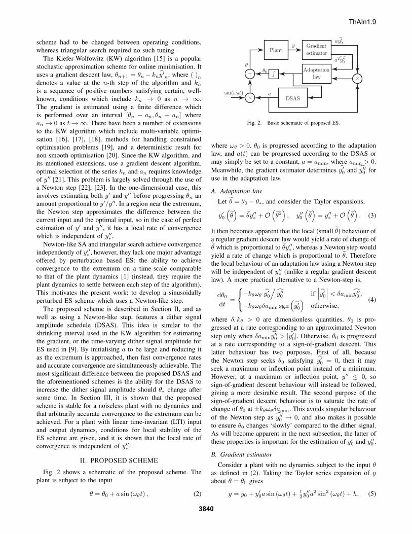
3842

Plant

yFo(s)Fi(s)θθi

f( )

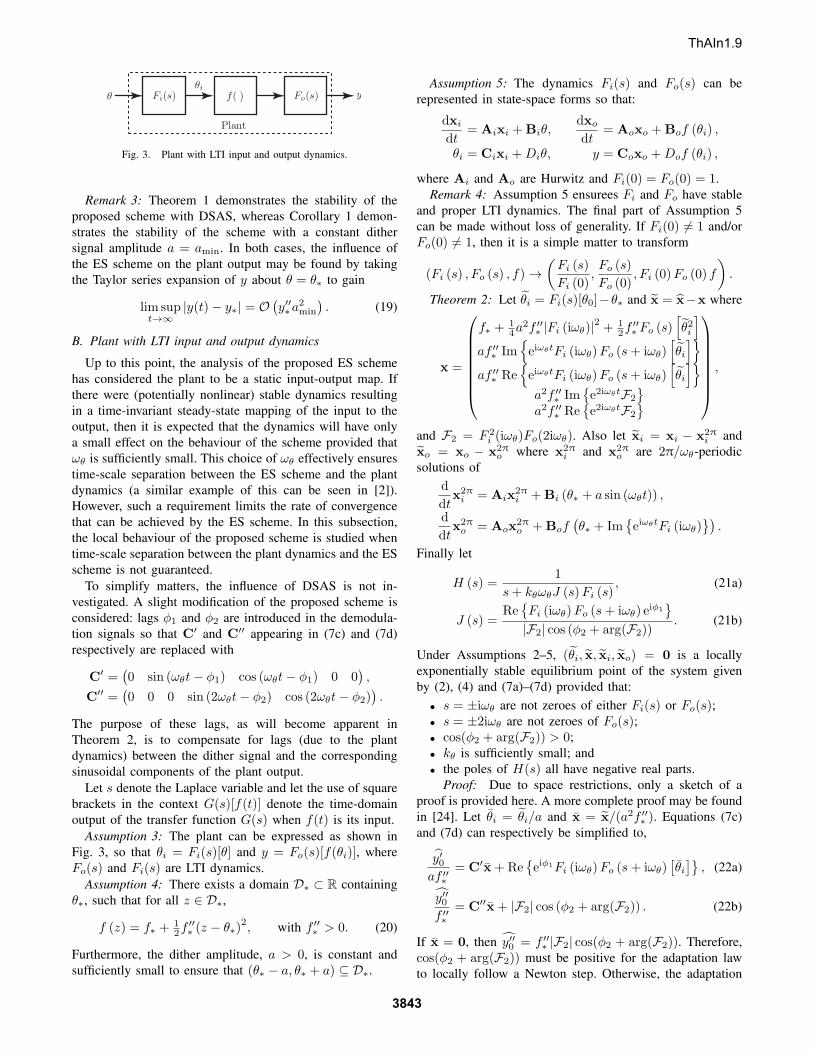
Fig. 3. Plant with LTI input and output dynamics.

Remark 3: Theorem 1 demonstrates the stability of the

proposed scheme with DSAS, whereas Corollary 1 demon-

strates the stability of the scheme with a constant dither

signal amplitude a = amin. In both cases, the influence of

the ES scheme on the plant output may be found by taking

the Taylor series expansion of y about � = �∗ to gain

lim supt→∞

∣y(t)− y∗∣ = O(y′′∗a2min

). (19)

B. Plant with LTI input and output dynamics

Up to this point, the analysis of the proposed ES scheme

has considered the plant to be a static input-output map. If

there were (potentially nonlinear) stable dynamics resulting

in a time-invariant steady-state mapping of the input to the

output, then it is expected that the dynamics will have only

a small effect on the behaviour of the scheme provided that

!� is sufficiently small. This choice of !� effectively ensures

time-scale separation between the ES scheme and the plant

dynamics (a similar example of this can be seen in [2]).

However, such a requirement limits the rate of convergence

that can be achieved by the ES scheme. In this subsection,

the local behaviour of the proposed scheme is studied when

time-scale separation between the plant dynamics and the ES

scheme is not guaranteed.

To simplify matters, the influence of DSAS is not in-

vestigated. A slight modification of the proposed scheme is

considered: lags �1 and �2 are introduced in the demodula-

tion signals so that C′ and C

′′ appearing in (7c) and (7d)

respectively are replaced with

C′ =

(0 sin (!�t− �1) cos (!�t− �1) 0 0

),

C′′ =

(0 0 0 sin (2!�t− �2) cos (2!�t− �2)

).

The purpose of these lags, as will become apparent in

Theorem 2, is to compensate for lags (due to the plant

dynamics) between the dither signal and the corresponding

sinusoidal components of the plant output.

Let s denote the Laplace variable and let the use of square

brackets in the context G(s)[f(t)] denote the time-domain

output of the transfer function G(s) when f(t) is its input.

Assumption 3: The plant can be expressed as shown in

Fig. 3, so that �i = Fi(s)[�] and y = Fo(s)[f(�i)], where

Fo(s) and Fi(s) are LTI dynamics.

Assumption 4: There exists a domain D∗ ⊂ ℝ containing

�∗, such that for all z ∈ D∗,

f (z) = f∗ +12f

′′

∗(z − �∗)

2, with f ′′

∗> 0. (20)

Furthermore, the dither amplitude, a > 0, is constant and

sufficiently small to ensure that (�∗ − a, �∗ + a) ⊆ D∗.

Assumption 5: The dynamics Fi(s) and Fo(s) can be

represented in state-space forms so that:

dxi

dt= Aixi +Bi�,

dxo

dt= Aoxo +Bof (�i) ,

�i = Cixi +Di�, y = Coxo +Dof (�i) ,

where Ai and Ao are Hurwitz and Fi(0) = Fo(0) = 1.

Remark 4: Assumption 5 ensurees Fi and Fo have stable

and proper LTI dynamics. The final part of Assumption 5

can be made without loss of generality. If Fi(0) ∕= 1 and/or

Fo(0) ∕= 1, then it is a simple matter to transform

(Fi (s) , Fo (s) , f) →(Fi (s)

Fi (0),Fo (s)

Fo (0), Fi (0)Fo (0) f

).

Theorem 2: Let �i = Fi(s)[�0]−�∗ and x = x−x where

x =

⎛⎜⎜⎜⎜⎜⎜⎜⎝

f∗ +14a

2f ′′

∗∣Fi (i!�)∣2 + 1

2f′′

∗Fo (s)

[�2i

]

af ′′

∗Im

{ei!�tFi (i!�)Fo (s+ i!�)

[�i

]}

af ′′

∗Re

{ei!�tFi (i!�)Fo (s+ i!�)

[�i

]}

a2f ′′

∗Im

{e2i!�tℱ2

}

a2f ′′

∗Re

{e2i!�tℱ2

}

⎞⎟⎟⎟⎟⎟⎟⎟⎠

,

and ℱ2 = F 2i (i!�)Fo(2i!�). Also let xi = xi − x

2πi and

xo = xo − x2πo where x

2πi and x

2πo are 2π/!�-periodic

solutions of

d

dtx2πi = Aix

2πi +Bi (�∗ + a sin (!�t)) ,

d

dtx2πo = Aox

2πo +Bof

(�∗ + Im

{ei!�tFi (i!�)

}).

Finally let

H (s) =1

s+ k�!�J (s)Fi (s), (21a)

J (s) =Re

{Fi (i!�)Fo (s+ i!�) e

i�1

}

∣ℱ2∣ cos (�2 + arg(ℱ2)). (21b)

Under Assumptions 2–5, (�i, x, xi, xo) = 0 is a locally

exponentially stable equilibrium point of the system given

by (2), (4) and (7a)–(7d) provided that:

∙ s = ±i!� are not zeroes of either Fi(s) or Fo(s);∙ s = ±2i!� are not zeroes of Fo(s);∙ cos(�2 + arg(ℱ2)) > 0;

∙ k� is sufficiently small; and

∙ the poles of H(s) all have negative real parts.

Proof: Due to space restrictions, only a sketch of a

proof is provided here. A more complete proof may be found

in [24]. Let �i = �i/a and x = x/(a2f ′′

∗). Equations (7c)

and (7d) can respectively be simplified to,

y′0af ′′

∗

= C′x+Re

{ei�1Fi (i!�)Fo (s+ i!�)

[�i]}

, (22a)

y′′0f ′′

∗

= C′′x+ ∣ℱ2∣ cos (�2 + arg(ℱ2)) . (22b)

If x = 0, then y′′0 = f ′′

∗∣ℱ2∣ cos(�2 + arg(ℱ2)). Therefore,

cos(�2 + arg(ℱ2)) must be positive for the adaptation law

to locally follow a Newton step. Otherwise, the adaptation

ThAIn1.9

3843

law would follow a sign-of-gradient descent and, at best,

�i would chatter about zero. Substituting (7a) into (7b) and

(22a)–(22b) into (4) and linearising each resulting equation

about (�i, x, xi, xo) = 0 respectively yields

d�idt

= −k�FiJ (s)[�i]− k�Fi (s) [C

′x]

∣ℱ2∣ cos (�2 + arg(ℱ2)), (23)

dx

dt= Axx+ L�x (t)− Re

{ΓFo (s+ i!�)

[d�idt

]}(24)

where Γ = (0 −i 1 0 0)TFi(i!�) exp(i!�t) and �x(t)consists of terms that decay to zero independently of �iand xi. Therefore, �x(t) does not affect the local stability

of the ES scheme and is ignored for the remainder of this

analysis. If x = 0 in (23), then the dynamics of �i are given

by H(s), and �i converges to zero if the poles of H(s) all

have negative real parts. Similarly from (24), if �i = 0, then

x converges to zero under Assumption 2. Therefore (23)

and (24) can be thought of as two interconnected systems

which are independently stable. If the interconnections are

sufficiently weak, then the ES scheme will remain stable.

Theorem 9.2 in [25] quantifies the conditions under which

the interconnections can be considered sufficiently weak. In

this case, stability of the ES scheme can be guaranteed if k�is sufficiently small. Theorem 2 follows directly.

Remark 5: The local convergence of �i to zero is inde-

pendent of f ′′

∗since H(s) is independent of f ′′

∗.

Remark 6: Consider the quantity k� where

k�k�

= J (0)Fi (0) =∣ℱ1∣ cos (�1 + arg(ℱ1))

∣ℱ2∣ cos (�2 + arg(ℱ2)),

and ℱ1 = Fi(i!�)Fo(i!�). If Ω� := k�!� is sufficiently

small, then H(s) has a dominant pole at s = −Ω�+O(Ω2�).

This allows the final dot-point of Theorem 2 to be tested

more easily, but effectively restricts the dynamics of �ito be well-separated not only from the gradient estimator

dynamics, but also from the plant dynamics.

Remark 7: When �1 = �2 = 0 and Fi(s) = Fo(s) = 1,

H(s) has a single pole at s = −k�!�. If Ω� is small

(see Remark 6) and non-trivial dynamics are introduced,

that pole is shifted to a location near s = −k�!�. If

k� < 0, then the dynamics will destabilise the system. This

occurs because sgn(y′0) ∕= sgn(y′0) about the equilibrium

point. It follows that the scheme will ‘climb’ the plant map

rather than descend it as intended. If k� < k�, then slower

convergence of �i to zero will be observed than in the

absence of dynamics. If k� > k�, faster convergence will

be observed, however, the region for which the adaptation

law follows a Newton-step will decrease. For fixed !�, the

influence of the pole shift from −k�!� to −k�!� may be

compensated through selection of a different value of k� or

through suitable selection of �1 and �2.

IV. CONCLUSIONS

An ES scheme using a Newton-like adaptation law and

DSAS was developed and shown to achieve convergence of

the control input to a small neighbourhood of the extremum

from a potentially infinite domain of initial conditions. Fur-

thermore, for a plant with LTI input and output dynamics,

conditions for local stability of the ES scheme (without

DSAS) were found and it was shown that local convergence

of the control input is independent of y′′∗

. In part II of this

paper, the behaviour of the proposed ES scheme is further

explored in both numerical and experimental tests.

REFERENCES

[1] K. B. Ariyur and M. Krstic, Real-Time Optimization by Extremum-

Seeking Control. John Wiley & Sons, 2003.[2] M. Krstic and H. Wang, “Stability of extremum seeking feedback for

general nonlinear dynamic systems,” Automatica, vol. 36, pp. 595–601, 2000.

[3] R. N. Banavar, D. F. Chichka, and J. L. Speyer, “Convergence andsynthesis issues in extremum-seeking control,” in Proceedings of the

American Control Conference, 2000, pp. 438–443.[4] M. A. Rotea, “Analysis of multivariable extremum seeking algo-

rithms,” in Proceedings of the American Control Conference, 2000,pp. 433–437.

[5] G. C. Walsh, “On the application of multi-parameter extremum seekingcontrol,” in Proceedings of the American Control Conference, 2000,pp. 411–415.

[6] J.-Y. Choi, M. Krstic, K. Ariyur, and J. S. Lee, “Extremum seekingcontrol for discrete time systems,” IEEE T. Automat. Contr., vol. 47,pp. 318–323, 2002.

[7] Y. Tan, D. Nesic, and I. Mareels, “On non-local stability properties ofextremum seeking control,” Automatica, vol. 42, pp. 889–903, 2006.

[8] D. Nesic, Y. Tan, and I. Mareels, “On the choice of dither in extremumseeking systems: a case study,” in Proceedings of the IEEE Conference

on Decision and Control, 2006, pp. 2789–2794.[9] Y. Tan, D. Nesic, I. Mareels, and A. Astolfi, “On global extremum

seeking in the presence of local extrema,” in Proceedings of the IEEE

Conference on Decision and Control, 2006, pp. 5663–5668.[10] C. Manzie and M. Krstic, “Extremum seeking with stochastic pertur-

bations,” IEEE T. Automat. Contr., vol. 54, pp. 580–585, 2009.[11] M. Krstic, “Performance improvement and limitations in extremum

seeking control,” Syst. Control Lett., vol. 39, pp. 313–326, 2000.[12] A. Banaszuk, K. B. Ariyur, M. Krstic, and C. A. Jacobsen, “An adap-

tive algorithm for control of thermoacoustic instability,” Automatica,vol. 40, pp. 1965–1972, 2004.

[13] Y. Zhang, “Stability and performance tradeoff with discrete timetriangular search minimum seeking,” in Proceedings of the American

Control Conference, 2000, pp. 423–427.[14] A. Banaszuk, Y. Zhang, and C. A. Jacobson, “Adaptive control of

combustion instability using extremum-seeking,” in Proceedings of the

American Control Conference, 2000, pp. 416–422.[15] J. Kiefer and J. Wolfowitz, “Stochastic estimation of a regression

function,” Ann. Math. Stat, vol. 23, pp. 462–466, 1952.[16] J. R. Blum, “Multidimensional stochastic approximation methods,”

Ann. Math. Stat, vol. 25, pp. 737–744, 1954.[17] H. J. Kushner and D. S. Clark, Stochastic approximation methods for

constrained and unconstrained systems. Springer-Verlag, 1978.[18] J. C. Spall, “Multivariate stochastic approximation using a simultane-

ous perturbation gradient,” IEEE T. Automat. Contr., vol. 37, no. 3,pp. 332–341, 1992.

[19] H. J. Kushner, “Stochastic approximation algorithms for constrainedoptmization problems,” Ann. Stat, vol. 2, no. 4, pp. 713–723, 1974.

[20] A. R. Teel, “Lyapunov methods in nonsmooth optimization, part II:persistently exciting finite differences,” in Proceedings of the IEEE

Conference on Decision and Control, 2000, pp. 118–123.[21] S. Yakowitz, P. L’Ecuyer, and F. Vazquez-Abad, “Global stochastic

optmization with low-dispersion point sets,” Oper. Res., vol. 48, no. 6,pp. 939–950, 2000.

[22] V. Fabian, “Stochastic approximation,” in Optimizing Methods in

Statistics. Academic Press, 1971, pp. 439–470.[23] J. C. Spall, “Adaptive stochastic approximation by the simultaneous

perturbation method,” IEEE T. Automat. Contr., vol. 45, no. 10, pp.1839–1853, 2000.

[24] W. H. Moase, C. Manzie, and M. J. Brear, “Newton-like extremum-seeking for the control of thermoacoustic instability,” IEEE T. Au-

tomat. Contr., (In press).[25] H. Khalil, Nonlinear systems, 3rd ed. Prentice Hall, 2002.

ThAIn1.9

3844