Myopia and Anchoring*

George-Marios Angeletos† Zhen Huo‡

March 21, 2020

Abstract

We offer a simple toolbox for understanding and quantifying the equilibrium effects of incomplete in-

formation. We first develop an observational equivalence between incomplete information and two

behavioral distortions: myopia, or extra discounting of the future; and anchoring of the current out-

come to the past outcome, as if there were habit. The distortions are larger when GE considerations

are more important, reflecting the role of higher-order uncertainty. We next show how to connect the

theory to evidence on expectations, giving new guidance on which moments of the expectations are

best suited for the purpose of disciplining the theory. We finally illustrate the quantitative potential

of informational frictions in the context of the New Keynesian Philips and Dynamic IS curves.

*We are grateful to three anonymous referees and an editor for extensive feedback, and to Chris Sims, Alexander Kohlhas,

Luigi Iovino, and Alok Johri for discussing our paper in, respectively, the 2018 NBER Monetary Economics meeting, the 2018

Cambridge/INET conference, the 2018 Hydra workshop, and the 2018 Canadian Macro Study Group. We also acknowledge use-

ful comments from Jaroslav Borovicka, Simon Gilchrist, Michael Golosov, Jennifer La’O, John Leahy, Kristoffer Nimark, Stephen

Morris, Mikkel Plagborg-Moller and seminar participants at the aforementioned conferences, Columbia, NYU, LSE, UCL, UBC,

Chicago Fed, Minneapolis Fed, Stanford, Carleton, Edinburgh, CUHK, the 2018 Duke Macro Jamboree, the 2018 Barcelona GSE

Summer Forum EGF Group, the 2018 SED Meeting, the 2018 China International Conference in Economics, and the 2018 NBER

Summer Institute. Angeletos acknowledges the support of the National Science Foundation under Grant Number SES-1757198.†MIT and NBER; angelet@mit.edu.‡Yale University; zhen.huo@yale.edu.

1 Introduction

What are the macroeconomics implications of informational frictions and higher-order uncertainty?

How do they relate to other sources of “stickiness”? And what is their quantitative potential? In this

paper we offer a simple toolbox for addressing these questions.1

We establish an observational equivalence between an economy featuring incomplete, heterogenous

information and a representative-agent, full-information variant featuring two behavioral distortions:

(i) myopia, or extra discounting of future outcomes; and (ii) anchoring of current outcomes to past out-

comes, or habit-like behavior. Both of these distortions are larger when GE considerations are more

important, as when there are strong input-output linkages behind the New Keynesian Philips curve or a

steep Keynesian cross behind the Dynamic IS curve. We extracts lessons for the relation between micro

and macro responses; connect to evidence on expectations; and offer a quantitative assessment.

Framework. Our starting point is a representative-agent model, in which an endogenous outcome

of interest, denoted by at , obeys the following law of motion:

at =ϕξt +δEt [at+1] , (1)

where ξt is the underlying stochastic impulse, or “fundamental”,ϕ> 0 and δ ∈ (0,1] are fixed scalars, and

Et [·] is the rational expectation of the representative agent.

In the textbook New Keynesian model, condition (1) could be both the New Keynesian Philips Curve

(NKPC), with at standing for inflation and ξt for the real marginal cost, or the Dynamic IS curve, with at

standing for aggregate spending and ξt for the real interest rate. Alternatively, this condition can be read

as an asset-pricing equation, with ξt standing for the asset’s dividend and at for its price.

We depart from these familiar, representative-agent benchmarks by letting people have incomplete

information about, or an imperfect “understanding” of, the state of Nature. The friction could be the

product of dispersed noisy information (Lucas, 1972), or a metaphor for cognitive constraints (Sims,

2003; Tirole, 2015). Crucially, the friction interferes with how agents adjust their beliefs not only about

the exogenous impulse but also about the behavior of others (Morris and Shin, 1998; Woodford, 2003).

Main theoretical result. Under appropriate assumptions, the incomplete-information economy is

observationally equivalent to a representative-agent one in which condition (1) is modified as follows:

at =ϕξt +δω f Et [at+1]+ωb at−1, (2)

for some ω f < 1 and ωb > 0. The first distortion (ω f < 1) represents myopia towards the future, the sec-

ond (ωb > 0) anchors current outcomes to past outcomes. The one dulls the forward-looking behavior,

the other adds a backward-looking element akin to habit or adjustment costs.

1Ours is certainly not the first paper to deal with these questions. The key works we build on and our marginal contributionsare discussed below. A review of the related literature can be found in Angeletos and Lian (2016).

1

Both of these distortions increase, not only with the level of noise, but also with a parameter that

governs the strategic complementarity or the GE feedback—think of the extent of input-output linkages

behind the NKPC, or the slope of the Keynesian cross behind the the Dynamic IS curve. This property

offers guidance on how the friction works, how its empirical footprint differs from that of true habit and

adjustment costs, and how to interpret and use the available evidence on expectations.

Underlying insights and marginal contribution. Our observational-equivalence result encapsulates

two insights that have previously been documented in the literature, albeit in different forms. The first

insight is that gradual learning manifests as “stickiness” in the aggregate dynamics (Sims, 2003; Mankiw

and Reis, 2002; Woodford, 2003; Nimark, 2008). The second insight is that higher-order uncertainty

causes agents to act as if they discount forward-looking GE considerations (Angeletos and Lian, 2018).

Relative to this prior literature, our theoretical contribution contains: (i) the bypassing of the curse of

dimensionality in higher-order beliefs; (ii) the existence, uniqueness and analytical characterization of

the equilibrium; and (iii) the observational-equivalence result. This in turn paves the way to our applied

contribution, which itself consists of: (iv) a few insights about the relation between micro and macro;

(v) some guidance on which evidence on expectations is best suited for the purpose of disciplining the

theory; and (vi) two quantitative illustrations, one for inflation and another for consumption.

DSGE and micro to macro. Our observational equivalence offers the sharpest to-date illustration of

how informational frictions may substitute for the more dubious forms of sluggish adjustment employed

in the DSGE literature: the backward-looking element in condition (2) is akin to that introduced by habit

persistence in consumption, adjustment costs to investment, or the Hybrid NKPC.

In addition, by tying both ωb and ω f to the GE feedback, our result highlights how these as-if distor-

tions may be endogenous to policies and market structures that regulate this feedback. This has novel

implications for, inter alia, how the inertia in inflation may relate to the slope of the Taylor rule and the

extent of input-output linkages.

Relatedly, our analysis yields the following, seemingly paradoxical, conclusion: more responsiveness

at the micro level comes together with more sluggishness at the macro level. For instance, a larger de-

gree of price flexibility for firms maps to more sluggishness in aggregate inflation, and a higher marginal

propensity to consume (MPC) out of income for households maps to more habit-like persistence in ag-

gregate consumption. In both cases, the reason is the larger micro-level responsiveness is associated

with a stronger GE feedback and hence a larger bite of higher-order uncertainty.

Connection to evidence on expectations. Our observational equivalence result facilitates a simple

quantitative strategy. We show how estimates ofω f andωb can readily be obtained by combining existing

knowledge about the relevant GE parameters with an appropriate moment of the average forecasts, such

as that estimated in Coibion and Gorodnichenko (2015), or CG for short. This moment is the coefficient

of the regression of the average forecast errors on past forecast revisions.

2

The basic intuition is similar to that articulated in CG: a higher value for the aforementioned coef-

ficient indicates more sluggish adjustment in expectations, or a larger informational friction. But there

is a crucial subtlety: both the structural interpretation of this moment and its mapping to the macroe-

conomic dynamics is modulated by the GE feedback. When this feedback is strong enough, a modest

friction by the CG metric may masquerade a large friction in terms of the implied values for ω f and ωb .

At the same time, we explain why the moment of the average (consensus) forecasts estimated in CG is

more “reliable” for our purposes than the individual-level counterpart estimated in Bordalo et al. (2018)

and Kohlhas and Broer (2019), or other moments of the individual forecasts such as the cross-sectional

dispersion of forecast errors. We further show how our mapping from the CG moment to the distortions

of interest may be robust to richer information structures, including endogenous public signals.

Applications to inflation and consumption. We conclude with a few concrete illustrations of how

our “toolbox” can be used to assess the macroeconomic effects of informational frictions.

First, we establish, on the basis of the aforementioned mapping from the CG moment to the pair

(ωb ,ω f ), that the level of friction implicit in surveys of inflation forecasts is large enough to alone ra-

tionalize existing estimates of the Hybrid NKPC (Galí and Gertler, 1999; Galí, Gertler, and Lopez-Salido,

2005). This complements prior work that had hypothesized this for some level of noise but had not dis-

ciplined the theory with expectations data (Nimark, 2008; Woodford, 2003).2

Second, we show that, under the lens of the theory, most of the friction’s quantitative effect reflects

the anchoring of the expectations of the behavior of others (future inflation) rather than the expectations

of the fundamental (real marginal cost). This echoes a recurring theme of our paper, which is that the

friction works in large part by arresting GE feedbacks.

Third, turning to the demand side, we show that, for a plausible calibration, the level of habit-like per-

sistence induced by the informational friction is comparable to that used in the DSGE literature (Chris-

tiano, Eichenbaum, and Evans, 2005; Smets and Wouters, 2007). This helps reconcile the gap between the

levels of habit required to match the macroeconomic time series and the much smaller levels estimated

in microeconomic data (Havranek, Rusnak, and Sokolova, 2017).3

Finally, we use a tractable HANK-like extension of our model to shed new light on how heterogeneity

may interact with informational frictions. In particular, we show that a positive cross-sectional correla-

tion between MPC and income cyclicality, like that documented empirically in Patterson (2019), ampli-

fies the information-driven sluggishness in the response of aggregate spending to monetary policy.

2Related is also the literature on adaptive learning (Sargent, 1993; Evans and Honkapohja, 2012; Marcet and Nicolini, 2003).This literature, too, allows for the anchoring of current outcomes to past outcomes; see, in particular, Carvalho et al. (2017)for an application to inflation. The anchoring found in our paper has three distinct qualities: it is consistent with rationalexpectations; it is tied to the strength of the GE feedback; and it is directly comparable to that found in the DSGE literature.

3Complementary in this respect are Carroll et al. (2020) and Auclert, Rognlie, and Straub (2020).

3

2 Framework

In this section we set up our framework and illustrate its applicability. We also discuss the essence of the

friction we are after and the complexity we aim at bypassing.

2.1 Basic ingredients

Time is discrete, indexed by t ∈ {0,1, ...}, and there is a continuum of players, indexed by i ∈ [0,1]. In each

period t , each agent i chooses an action ai ,t ∈ R. The corresponding average action is denoted by at .

Best responses admit the following recursive formulation:

ai ,t = Ei ,t[ϕξt +βai ,t+1 +γat+1

](3)

where ξt is the underlying exogenous fundamental, Ei ,t [·] denotes the player’s expectation in period

t , and (ϕ,β,γ) are parameters, with ϕ > 0, γ ∈ [0,δ), β = δ− γ, and δ ∈ (0,1). As it will become clear

shortly, δ = β+γ parameterizes the agent’s overall concern about the future and γ the component of

it that reflects GE, or strategic, considerations. We further assume that individual expectations satisfy

the law of iterated expectations along with the following limit properties: limk→∞βkEi ,t [ai ,t+k ] = 0,

limk→∞βkEi ,t [ξt+k ] = 0, and limk→∞βkEi ,t [at+k ] = 0.4 Iterating on condition (3) then yields the follow-

ing extensive-form representation of the best response of player i in period t :

ai ,t =∞∑

k=0βkEi ,t

[ϕξt+k

]+γ ∞∑k=0

βkEi ,t [at+k+1] . (4)

While the recursive form of the best responses seen in condition (3) is relatively more convenient to

work with, the extensive form given in condition (4) highlights that a player’s optimal behavior at any

given point of time depends on her expectations of the entire future paths of the fundamental and of the

average action. Aggregating it also yields the following equilibrium restriction:

at =ϕ∞∑

k=0βkEt [ξt+k ]+γ

∞∑k=0

βkEt [at+k+1] , (5)

where Et [.] denotes the average expectation in the population. This condition in turn is useful for two

purposes. First, it highlights the fixed-point relation between the equilibrium outcome and the ex-

pectations of it, whereby higher-order beliefs come into play. And second, it helps nest incomplete-

information versions of the building blocks of the New Keynesian model.5

4The first property can be understood as the transversality condition of a dynamic optimization problem whose Euler con-dition is given by (3). The second represents a restriction on the fundamental process, trivially satisfied if ξt is either boundedor a random walk. The third represents a equilibrium refinement standard in infinite-horizon settings.

5 The same best-response structure is assumed in Angeletos and Lian (2018). But whereas that paper considers a non-stationary setting where ξt is fixed at zero for all t 6= T , for some given T ≥ 1, we consider a stationary setting in which ξt variesin all t and, in addition, there is gradual learning over time. Our framework also resembles the beauty contests consideredby Morris and Shin (2002), Woodford (2003), Angeletos and Pavan (2007), Bergemann and Morris (2013), and Huo and Pedroni

4

2.2 Complete information and beyond

Suppose momentarily that all agents have complete information, meaning that they share the same (al-

though possibly noisy) information and this fact is itself common knowledge. The economy then admits

a representative agent. That is, ai ,t = at and Ei ,t = Et , where Et stands for the representative agent’s

expectation. In this benchmark, condition (3) reduces to the following:

at = Et [ϕξt +δat+1], (6)

which may correspond to the textbook versions of the Dynamic IS and New Keynesian Philips curves, or

an elementary asset-pricing equation. Accordingly, the equilibrium outcome is given by

at =ϕ∞∑

h=0δhEt [ξt+h]. (7)

This can be read as “inflation equals the present discounted value of real marginal costs” or “the asset’s

price equals the present discounted value of its dividends.”

Clearly, only the composite parameterδ=β+γ enters the determination of the equilibrium outcome:

its decomposition betweenβ and γ is irrelevant. As made clear in Section 2.4 below, this underscores that

the decomposition between PE and GE considerations is immaterial in this benchmark. Furthermore,

the outcome is pinned down by the expectations of the fundamental alone.

These properties hold because this benchmark imposes that agents can reason about the behavior of

others with the same ease and precision as they can reason about their own behavior. Conversely, intro-

ducing incomplete (differential) information and higher-order uncertainty amounts to accommodating

a friction in how agents reason about the behavior of others, or about GE.

The specific information structure assumed, which aims at maximizing tractability and clarity, is

spelled out in Section 3.1. In the remainder of this section, we first illustrate how our setting can nest

incomplete-information extensions of the Dynamic IS and the New Keynesian Philips curves; we then

discuss the essence of the friction we are after and the complexity we wish to bypass.

2.3 Two Examples: Dynamic IS and NKPC

The (log-linearized) New Keynesian model boils down to two forward-looking equations, the Dynamic

IS curve and the New Keynesian Philips Curve (NKPC), along with a specification of monetary policy.

(2019). However, because behavior is not forward-looking in these settings, the relevant higher-order beliefs are those regardingthe concurrent beliefs of others. By contrast, the relevant higher-order beliefs in our setting are those regarding the future beliefsof others, as in Allen, Morris, and Shin (2006), Morris and Shin (2006) and Nimark (2017). The best-response structure assumedin the latter set of papers is herein nested by restricting β= 0. As discussed in Section 2.4, allowing β> 0 significantly increasesthe dimensionality and complexity of the relevant higher-order beliefs.

5

The familiar, representative-agent versions of these equations are given by, respectively,

ct = Et [−ςrt + ct+1] and πt = Et [κmct +χπt+1],

where ct is aggregate consumption, rt is the real interest rate, πt is inflation, mct is the real marginal

cost, ς > 0 is the elasticity of intertemporal substitution, κ ≡ (1−χθ)(1−θ)θ is the slope of the Philips curve,

θ ∈ (0,1) is the Calvo parameter, χ ∈ (0,1) is the subjective discount factor, and Et is the expectation of the

representative agent. The first equation describes how aggregate spending responds to the real interest

rate, the second how inflation responds to the real marginal cost or the output gap. Clearly, both of these

conditions are nested in (6), the representative-agent restriction of our model.

Relaxing the common-knowledge foundations of the New Keynesian model along the lines of An-

geletos and Lian (2018) yields the following incomplete-information extensions of these equations:

ct =−ς∞∑

k=0χkEt [rt+k ]+ (1−χ)

∞∑k=1

χk−1Et [ct+k ], (8)

πt = κ∞∑

k=0(χθ)kEt [mct+k ]+χ(1−θ)

∞∑k=0

(χθ)kEt [πt+k+1] , (9)

where Et denotes the average expectation of the consumers in (8) and that of the firms in (9). The first

equation is nested in condition (5) by letting at = ct , ξt = rt ,ϕ=−ς,β=χ, γ= 1−χ, and δ= 1; the second

by letting at =πt , ξt = mct , ϕ= κ, β=χθ, γ=χ(1−θ) and δ=χ.

To understand condition (8), recall that the Permanent Income Hypothesis gives consumption as a

function of the present discounted value of income. Incorporating variation in the real interest rate and

heterogeneity in beliefs, and using the fact that aggregate income equals aggregate spending in equilib-

rium, yields condition (8). Finally, note that 1−χ measures the marginal propensity to consume (MPC)

out of income. The property that γ= 1−χ therefore means that, in this context, γ captures the slope of

the Keynesian cross, or the GE feedback between spending and income.6

To understand condition (9), recall that a firm’s optimal reset price is given by the present discounted

value of its nominal marginal cost. Aggregating across firms and using the identity that ties inflation

to the average rest price yields condition (9). When all firms share the same, rational expectations, this

condition reduces to the familiar, textbook version of the NKPC. Away for that benchmark, condition (9)

reveals the precise manner in which expectations of future inflation (the behavior of the firms) feed into

current inflation. Note in particular that γ= χ(1−θ), which means that the effective degree of strategic

complementarity increases with the frequency of price adjustment. This is because the feedback from

the expectations of future inflation to current inflation increases when a higher fraction of firms are able

to adjust their prices today on the basis of such expectations.

6See Section 6 for a perpetual-youth, overlapping-generations extension, which disentangles the MPC from the discountfactor and makes clear that γ is given by the former, not the latter. This corroborates the interpretation of γ as a proxy for theslope of the Keynesian cross.

6

2.4 Higher-Order Beliefs: The Wanted Essence and the Unwanted Complexity

An integral part of our contribution is to relate higher-order uncertainty to how agents reason about

GE and, subsequently, to elaborate on the empirical content of this perspective. To this goal, we revisit

condition (5), which allows the following decomposition of the aggregate outcome:

at =ϕ∞∑

k=0βkEt [ξt+k ]︸ ︷︷ ︸

PE component

+γ∞∑

k=0βkEt [at+k+1]︸ ︷︷ ︸

GE component

. (10)

We label the first term as the PE component because it captures the agents’ response to any innovation

holding constant their expectations about the endogenous outcome; the additional change triggered by

any adjustment in these expectations, or the second term above, represents the GE component.

To illustrate how this decomposition matters when, and only when, information is incomplete, con-

sider the following example. There are two economies, labeled A and B , that share the same process

for ξt , the same information structure, and the same δ ≡ β+γ, but have a different mixture of β and γ.

Economy A features β= δ and γ= 0, which means that GE considerations are entirely absent. Economy

B features β= 0 and γ= δ, which corresponds to “maximal” GE considerations.

In economy A, condition (5) becomes at = ϕ∑∞

k=0δkEt [ξt+k ], that is, only the first-order beliefs of

the fundamental matter. This is similar to the representative-agent benchmark, except that the repre-

sentative agent’s expectations are replaced by the average expectations in the population. In economy

B , instead, condition (5) reduces to at =ϕEt [ξt ]+δEt [at+1] and recursive iteration yields

at =ϕ∞∑

h=1δhF

ht [ξt+h−1] , (11)

where, for any variable X , F1t [X ] ≡ Et [X ] denotes the average first-order forecast of X and, for all h ≥ 2,

Fht [X ] ≡ Et

[F

h−1t+1 [X ]

]denotes the corresponding h-th order forecast. The key difference from both the

representative-agent benchmark and economy A is the emergence of such higher-order beliefs. These

represent GE considerations, or the agents’ reasoning about the behavior of others.7

The logic extends to the general case, in which both β and γ are positive. The only twist is that the

relevant set of higher-order beliefs is significantly richer than that seen in condition (11). Indeed, let

ζt ≡∑∞τ=0β

τξt+τ and consider the following set of forward-looking, higher-order beliefs:

Et1 [Et2 [· · · [Eth [ζt+k ] · · · ]],

for any t ≥ 0, k ≥ 2, h ∈ {2, ...,k}, and {t1, t2, ..., th} such that t = t1 < t2 < ... < th = t +k. It is easy to show

that, when β> 0, the period-t outcome depends on all of these higher-order beliefs.

7With complete information (common knowledge), higher-order beliefs collapse to first-order beliefs. With incomplete in-formation (lack of common knowledge), higher-order beliefs depart from first-order beliefs. This formalizes the sense in whichincomplete information introduces a friction in how agents reason about others relative to how they reason about themselves.

7

To further appreciate the added complexity relative to the β = 0 case, note that, for any t and any

k ≥ 2, there are now k−1 types of second-order beliefs, plus (k−1)×(k−2)/2 types of third-order beliefs,

plus (k−1)×(k−2)×(k −3)/6 types of fourth-order beliefs, and so on. For instance, when k = 10 (thinking

about the outcome 10 periods later), there are 210 beliefs of the fourth order that are relevant when β> 0

compared to only one such belief when β= 0.

An integral part of our contribution is the complete bypassing of this complexity. The assumptions

that permit this bypassing are spelled out in the next section. They come at the cost of some generality,

in particular we abstract from the possible endogeneity of information.8 But they also bear significant

gains on both the theoretical and the quantitative front, which will become evident as we proceed.

3 The Equivalence Result

This section contains the core of our contribution. We introduce the assumptions that let us bypass the

complexity of higher-order beliefs and solve directly the rational-expectations fixed point, proceed to

develop our observation-equivalence result, and discuss the main insights encapsulated in it.

3.1 Specification

We henceforth make two assumptions. First, we let the fundamental ξt follow an AR(1) process:

ξt = ρξt−1 +ηt = 1

1−ρLηt , (12)

where ηt ∼ N (0,1) is the period-t innovation, L is the lag operator, and ρ ∈ (0,1) parameterizes the

persistence of the fundamental. Second, we assume that player i receives a new private signal in each

period t , given by

xi ,t = ξt +ui ,t , ui ,t ∼N (0,σ2), (13)

where σ ≥ 0 parameterizes the informational friction (the level of noise). The player’s information in

period t is the history of signals up to that period.

As anticipated in the previous section, these assumptions aim at minimizing complexity without sac-

rificing essence. Borrowing from the literature on rational inattention, we also invite a flexible interpre-

tation of our setting as one where fundamentals and outcomes are observable but cognitive limitations

makes agents act as if they observe the entire state of Nature with idiosyncratic noise.9 But instead of

endogenizing the structure of this noise, we fix it in a way that best serves our purposes.

8This abstraction seems the right benchmark for the purposes of our paper, including the connections built to the evidenceon expectations: this evidence helps discipline the theoretical mechanisms we are concerned with, but contains little guidanceon the degree or manner in which information may be endogenous.

9Indeed, note that the history of the outcome up to, and including, period t is measurable in ξt ≡ (ξ0, ...,ξt ), which definesthe aggregate state of Nature in period t . The corresponding Harsanyi type of agent i is x t

i ≡ (xi 0, ...., xi ,t ). It follows that theassumed signals represent signals not only of the fundamental but also of the outcome.

8

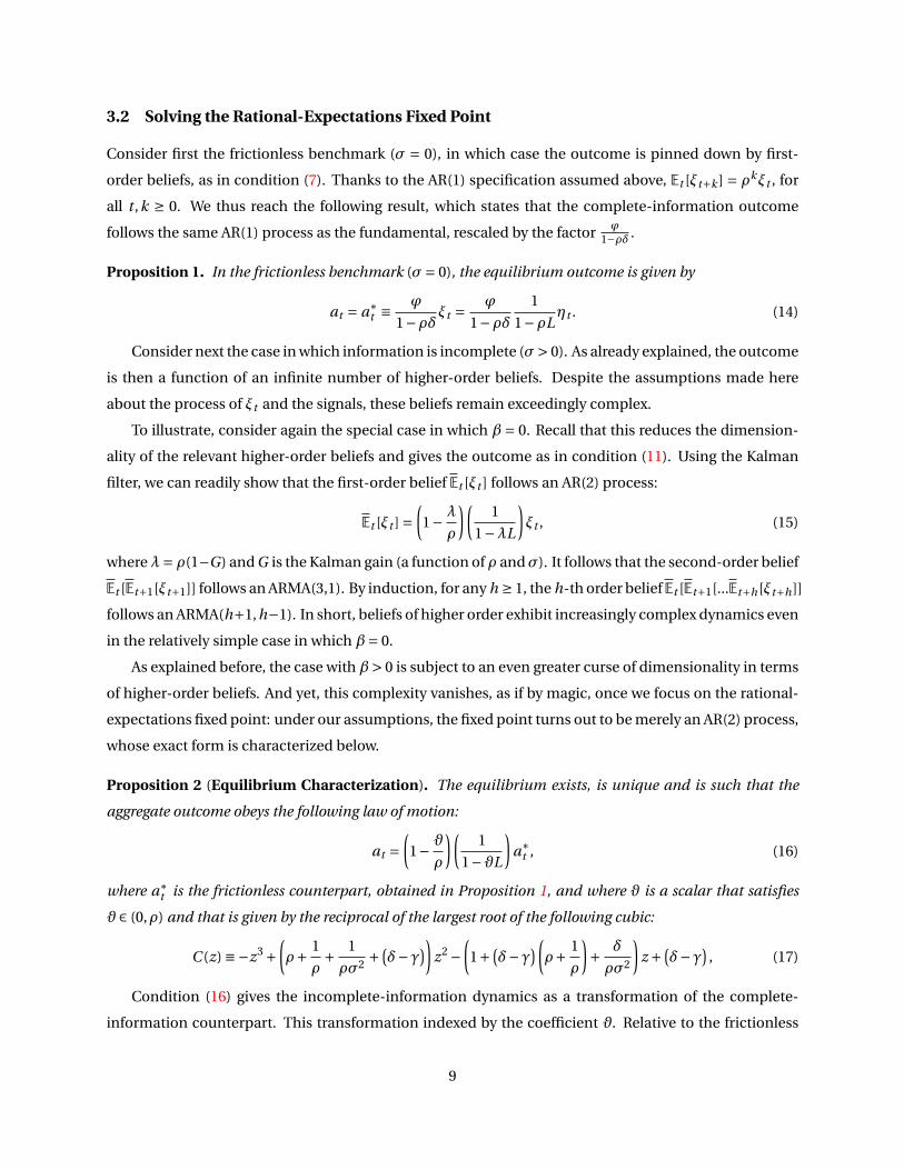
3.2 Solving the Rational-Expectations Fixed Point

Consider first the frictionless benchmark (σ = 0), in which case the outcome is pinned down by first-

order beliefs, as in condition (7). Thanks to the AR(1) specification assumed above, Et [ξt+k ] = ρkξt , for

all t ,k ≥ 0. We thus reach the following result, which states that the complete-information outcome

follows the same AR(1) process as the fundamental, rescaled by the factor ϕ1−ρδ .

Proposition 1. In the frictionless benchmark (σ= 0), the equilibrium outcome is given by

at = a∗t ≡ ϕ

1−ρδξt = ϕ

1−ρδ1

1−ρLηt . (14)

Consider next the case in which information is incomplete (σ> 0). As already explained, the outcome

is then a function of an infinite number of higher-order beliefs. Despite the assumptions made here

about the process of ξt and the signals, these beliefs remain exceedingly complex.

To illustrate, consider again the special case in which β= 0. Recall that this reduces the dimension-

ality of the relevant higher-order beliefs and gives the outcome as in condition (11). Using the Kalman

filter, we can readily show that the first-order belief Et [ξt ] follows an AR(2) process:

Et [ξt ] =(1− λ

ρ

)(1

1−λL

)ξt , (15)

whereλ= ρ(1−G) and G is the Kalman gain (a function of ρ andσ). It follows that the second-order belief

Et [Et+1[ξt+1]] follows an ARMA(3,1). By induction, for any h ≥ 1, the h-th order belief Et [Et+1[...Et+h[ξt+h]]

follows an ARMA(h+1,h−1). In short, beliefs of higher order exhibit increasingly complex dynamics even

in the relatively simple case in which β= 0.

As explained before, the case with β> 0 is subject to an even greater curse of dimensionality in terms

of higher-order beliefs. And yet, this complexity vanishes, as if by magic, once we focus on the rational-

expectations fixed point: under our assumptions, the fixed point turns out to be merely an AR(2) process,

whose exact form is characterized below.

Proposition 2 (Equilibrium Characterization). The equilibrium exists, is unique and is such that the

aggregate outcome obeys the following law of motion:

at =(1− ϑ

ρ

)(1

1−ϑL

)a∗

t , (16)

where a∗t is the frictionless counterpart, obtained in Proposition 1, and where ϑ is a scalar that satisfies

ϑ ∈ (0,ρ) and that is given by the reciprocal of the largest root of the following cubic:

C (z) ≡−z3 +(ρ+ 1

ρ+ 1

ρσ2 + (δ−γ))

z2 −(1+ (

δ−γ)(ρ+ 1

ρ

)+ δ

ρσ2

)z + (

δ−γ), (17)

Condition (16) gives the incomplete-information dynamics as a transformation of the complete-

information counterpart. This transformation indexed by the coefficient ϑ. Relative to the frictionless

9

benchmark (herein nested by ϑ = 0), a higher ϑ means both a smaller impact effect, captured by the

factor 1− ϑρ in condition (16), and a more sluggish build up over time, captured by the lag term ϑL.

In the rest of this section, we first offer some insight into the math behind the result. We then discuss

the economics encapsulated in it.

To understand the math, consider the special case in which β = 0. In this case, the outcome obeys

the following law of motion:

at =ϕEt [ξt ]+γEt [at+1] (18)

If we guess that at follows an AR(2), we have that Et [at+1] follows an ARMA(3,1). As already noted, Et [ξt ]

follows the AR(2) given in (15). The right-hand side of the above equation is therefore the sum of an AR(2)

and an ARMA(3,1). If the latter was arbitrary, this sum would have returned an ARMA(5,3), contradicting

our guess that at follows an AR(2). But the relevant ARMA(3,1) is not arbitrary.

Because the exogenous impulse behind at is ξt , one can safely guess that at inherits the root of ξt .

Hence, it better be that

at = b

(1−ϑL)(1−ρL)ηt = b

1−ϑLξt

for some b and ϑ. This implies that the three AR roots of the ARMA(3,1) process for Et [at+1] are the re-

ciprocals of ρ, ϑ and λ. As seen in (15), the roots of Et [ξt ] are the reciprocals of ρ and λ. These properties

guarantee that the sum in the right-hand side of (18) would be at most an ARMA(3,1) of the form

at = c(1−dL)

(1−ϑL)(1−ρL)(1−λL)ηt , (19)

where c and d are functions of b and ϑ.

The above step is true for arbitrary b and ϑ. For our guess to be correct, it’d better be that d = λ and

c = b. The first equation guarantees that the MA part and the last AR part cancel out, so that (19) reduces

to an AR(2) with the same roots as our initial guess; the second equation makes sure that the scale is also

the same. The first equation yields (17); the second yields b =(1− ϑ

ρ

)(ϕ

1−ρδ).

This is the crux of how the “magic” of the rational-expectations fixed point works. The proof pre-

sented in the Appendix follows a somewhat different path, which is more constructive, accommodates

β> 0, and can be extended to richer settings along the lines of Huo and Takayama (2018).

When γ = 0, GE considerations are absent, the outcome is pinned down by first-order beliefs, and

Proposition 2 holds with ϑ=λ, where λ is the same root as that seen in (15). When instead γ> 0, GE con-

siderations and higher-order beliefs come into play. As already noted, such beliefs follow complicated

ARMA processes of ever increasing orders. And yet, the equilibrium continues to follow a simple AR(2)

process. The only twist is that ϑ > λ, which, as mentioned above, means that the equilibrium outcome

exhibits less amplitude and more persistence than the first-order beliefs. This is the empirical footprint

of higher-order uncertainty, or of the kind of imperfect GE reasoning accommodated in our analysis.

10

In the sequel, we translate these properties in terms of our observational-equivalence result (Propo-

sition 3) and a few complementary results about the interaction of GE effects and incomplete informa-

tion (Propositions 5 and 6). The following corollary, which proves useful when connecting the theory to

evidence on expectations, is also immediate.

Corollary 1. Any moment of the joint process of the aggregate outcome, at , and of the average forecasts,

Et [at+k ] for all k ≥ 1, are functions of only the triplet (ϑ,λ,ρ), or equivalently of (γ,δ,ρ,σ).

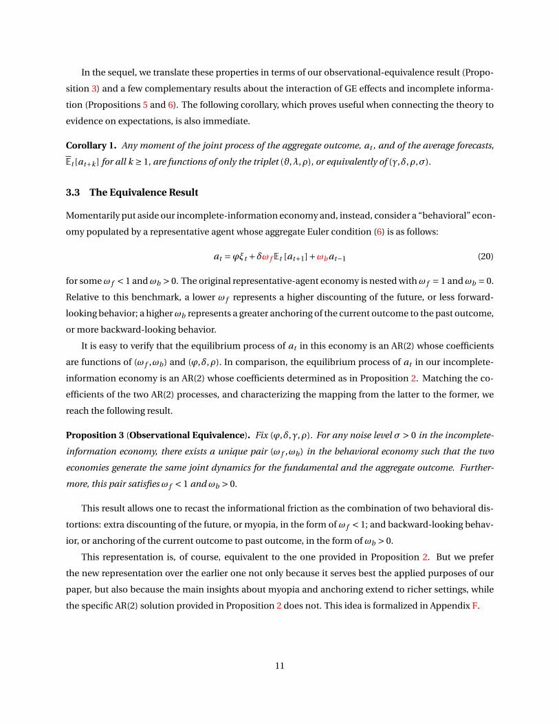
3.3 The Equivalence Result

Momentarily put aside our incomplete-information economy and, instead, consider a “behavioral” econ-

omy populated by a representative agent whose aggregate Euler condition (6) is as follows:

at =ϕξt +δω f Et [at+1]+ωb at−1 (20)

for someω f < 1 andωb > 0. The original representative-agent economy is nested withω f = 1 andωb = 0.

Relative to this benchmark, a lower ω f represents a higher discounting of the future, or less forward-

looking behavior; a higherωb represents a greater anchoring of the current outcome to the past outcome,

or more backward-looking behavior.

It is easy to verify that the equilibrium process of at in this economy is an AR(2) whose coefficients

are functions of (ω f ,ωb) and (ϕ,δ,ρ). In comparison, the equilibrium process of at in our incomplete-

information economy is an AR(2) whose coefficients determined as in Proposition 2. Matching the co-

efficients of the two AR(2) processes, and characterizing the mapping from the latter to the former, we

reach the following result.

Proposition 3 (Observational Equivalence). Fix (ϕ,δ,γ,ρ). For any noise level σ > 0 in the incomplete-

information economy, there exists a unique pair (ω f ,ωb) in the behavioral economy such that the two

economies generate the same joint dynamics for the fundamental and the aggregate outcome. Further-

more, this pair satisfies ω f < 1 and ωb > 0.

This result allows one to recast the informational friction as the combination of two behavioral dis-

tortions: extra discounting of the future, or myopia, in the form of ω f < 1; and backward-looking behav-

ior, or anchoring of the current outcome to past outcome, in the form of ωb > 0.

This representation is, of course, equivalent to the one provided in Proposition 2. But we prefer

the new representation over the earlier one not only because it serves best the applied purposes of our

paper, but also because the main insights about myopia and anchoring extend to richer settings, while

the specific AR(2) solution provided in Proposition 2 does not. This idea is formalized in Appendix F.

11

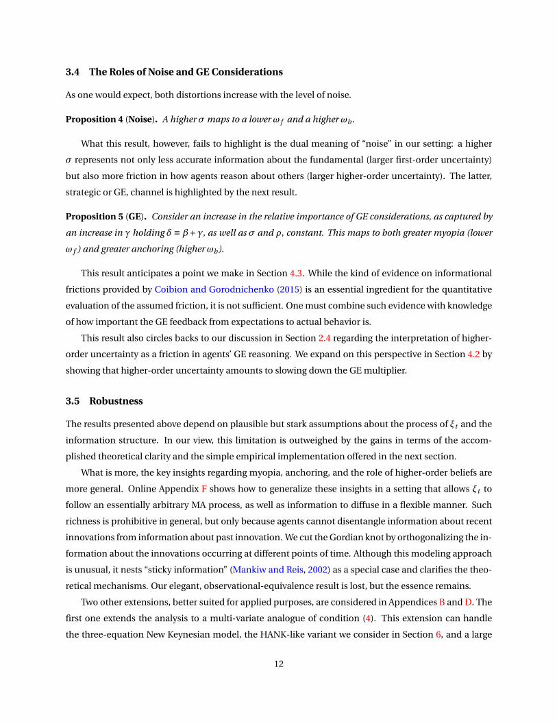
3.4 The Roles of Noise and GE Considerations

As one would expect, both distortions increase with the level of noise.

Proposition 4 (Noise). A higher σ maps to a lower ω f and a higher ωb .

What this result, however, fails to highlight is the dual meaning of “noise” in our setting: a higher

σ represents not only less accurate information about the fundamental (larger first-order uncertainty)

but also more friction in how agents reason about others (larger higher-order uncertainty). The latter,

strategic or GE, channel is highlighted by the next result.

Proposition 5 (GE). Consider an increase in the relative importance of GE considerations, as captured by

an increase in γ holding δ≡ β+γ, as well as σ and ρ, constant. This maps to both greater myopia (lower

ω f ) and greater anchoring (higher ωb).

This result anticipates a point we make in Section 4.3. While the kind of evidence on informational

frictions provided by Coibion and Gorodnichenko (2015) is an essential ingredient for the quantitative

evaluation of the assumed friction, it is not sufficient. One must combine such evidence with knowledge

of how important the GE feedback from expectations to actual behavior is.

This result also circles backs to our discussion in Section 2.4 regarding the interpretation of higher-

order uncertainty as a friction in agents’ GE reasoning. We expand on this perspective in Section 4.2 by

showing that higher-order uncertainty amounts to slowing down the GE multiplier.

3.5 Robustness

The results presented above depend on plausible but stark assumptions about the process of ξt and the

information structure. In our view, this limitation is outweighed by the gains in terms of the accom-

plished theoretical clarity and the simple empirical implementation offered in the next section.

What is more, the key insights regarding myopia, anchoring, and the role of higher-order beliefs are

more general. Online Appendix F shows how to generalize these insights in a setting that allows ξt to

follow an essentially arbitrary MA process, as well as information to diffuse in a flexible manner. Such

richness is prohibitive in general, but only because agents cannot disentangle information about recent

innovations from information about past innovation. We cut the Gordian knot by orthogonalizing the in-

formation about the innovations occurring at different points of time. Although this modeling approach

is unusual, it nests “sticky information” (Mankiw and Reis, 2002) as a special case and clarifies the theo-

retical mechanisms. Our elegant, observational-equivalence result is lost, but the essence remains.

Two other extensions, better suited for applied purposes, are considered in Appendices B and D. The

first one extends the analysis to a multi-variate analogue of condition (4). This extension can handle

the three-equation New Keynesian model, the HANK-like variant we consider in Section 6, and a large

12

class of forward-looking, incomplete-information networks. The second extension lets agents observe

a public signal on top of the private signals allowed so far. This anticipates an exercise conducted in

Section 5, where we show that the accommodation of public information may, paradoxically, intensify

the documented frictions once the theory is disciplined by the relevant evidence on expectations.

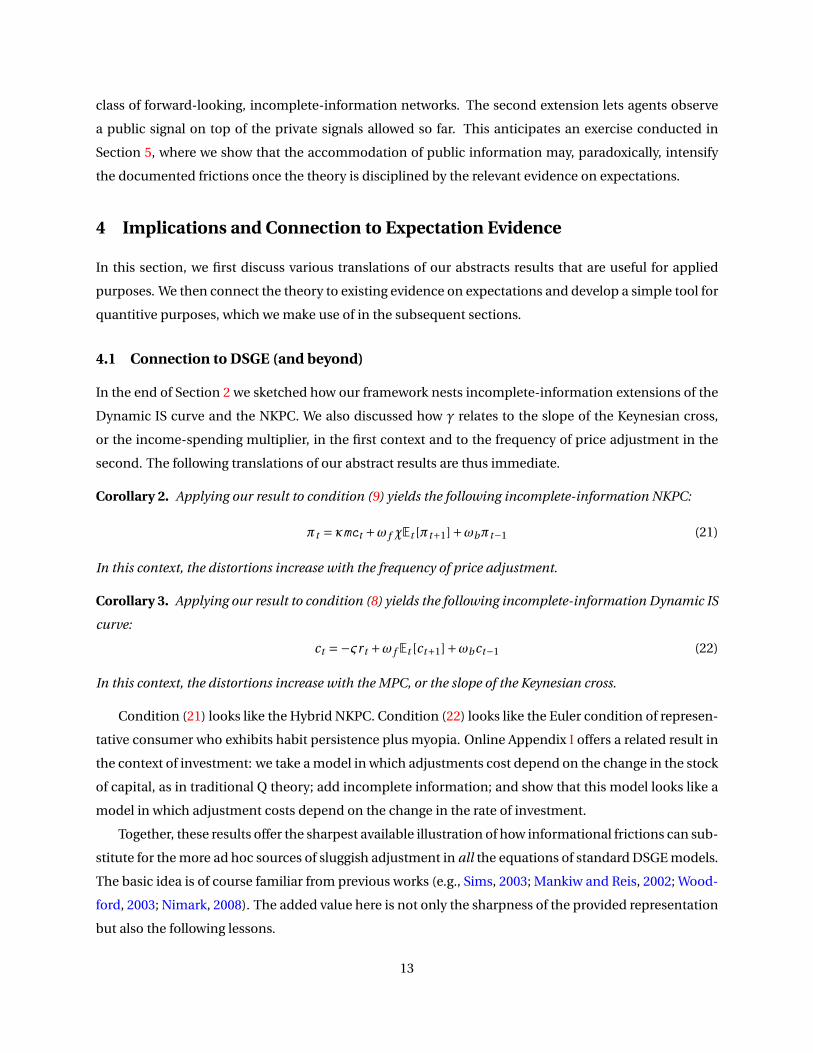
4 Implications and Connection to Expectation Evidence

In this section, we first discuss various translations of our abstracts results that are useful for applied

purposes. We then connect the theory to existing evidence on expectations and develop a simple tool for

quantitive purposes, which we make use of in the subsequent sections.

4.1 Connection to DSGE (and beyond)

In the end of Section 2 we sketched how our framework nests incomplete-information extensions of the

Dynamic IS curve and the NKPC. We also discussed how γ relates to the slope of the Keynesian cross,

or the income-spending multiplier, in the first context and to the frequency of price adjustment in the

second. The following translations of our abstract results are thus immediate.

Corollary 2. Applying our result to condition (9) yields the following incomplete-information NKPC:

πt = κmct +ω f χEt [πt+1]+ωbπt−1 (21)

In this context, the distortions increase with the frequency of price adjustment.

Corollary 3. Applying our result to condition (8) yields the following incomplete-information Dynamic IS

curve:

ct =−ςrt +ω f Et [ct+1]+ωbct−1 (22)

In this context, the distortions increase with the MPC, or the slope of the Keynesian cross.

Condition (21) looks like the Hybrid NKPC. Condition (22) looks like the Euler condition of represen-

tative consumer who exhibits habit persistence plus myopia. Online Appendix I offers a related result in

the context of investment: we take a model in which adjustments cost depend on the change in the stock

of capital, as in traditional Q theory; add incomplete information; and show that this model looks like a

model in which adjustment costs depend on the change in the rate of investment.

Together, these results offer the sharpest available illustration of how informational frictions can sub-

stitute for the more ad hoc sources of sluggish adjustment in all the equations of standard DSGE models.

The basic idea is of course familiar from previous works (e.g., Sims, 2003; Mankiw and Reis, 2002; Wood-

ford, 2003; Nimark, 2008). The added value here is not only the sharpness of the provided representation

but also the following lessons.

13

First, we show that, by intensifying the GE feedback from expectations of future inflation to current

inflation, higher price flexibility maps to more sluggishness in inflation. Although this prediction may be

hard to test, we find it to be an intriguing, new addition to the “paradoxes of flexibility.”

Second, we tie the habit-like persistence in consumption to the MPC, or the slope of the Keynesian

cross. This hints at the promise of incorporating incomplete information in the HANK literature. A

large part of this literature is devoted in boosting the Keynesian multiplier. In the light of our result, the

incorporation of incomplete information in that literature may offer a better account of the dynamics of

aggregate spending. We illustrate this point in Section 6.

Third, we offer a new rationale for why such distortions may loom large at the macro level even

if they are absent at the micro level. Previous work has emphasized that agents may naturally have less

information about aggregate shocks than about idiosyncratic shocks (Mackowiak and Wiederholt, 2009).

We add that higher-order uncertainty effectively amplifies the bite of the informational friction at the

macro level. Together, these insights help merge the pervasive gap between the macroeconomic and

microeconomic estimates of habit persistence in consumption, adjustment costs to investment, and

backward-looking in inflation. We expand on this point in Appendix E.

Fourth, by tying the macro-level distortions to GE feedbacks, we highlight how the former can be en-

dogenous to policies that regulate the later. For instance, a monetary policy that reacts more aggressively

to fluctuations in inflation maps, under the lens of our analysis, to a smaller backward-looking compo-

nent in the NKPC (that is, to less persistence in inflation for given persistence in the real marginal cost).

We discuss evidence supportive of this prediction in Section 5.

Fifth, we build a bridge to a literature that uses bounded rationality to arrest GE multipliers. We

expand on this point below.

Last but not least, we offer a simple strategy for quantifying the distortions of interest. We spell out

the elements of this strategy in Section 4.3 and put it at work in Section 5.

4.2 Arresting GE Multipliers

Recall that condition (10), which we reproduce below, allowed us to decompose the equilibrium outcome

in its PE and GE components:

at =ϕ∞∑

k=0βkEt [ξt+k ]︸ ︷︷ ︸

PE component

+γ∞∑

k=0βkEt [at+k+1]︸ ︷︷ ︸

GE component

. (23)

Recasting this decomposition in terms of the Impulse Response Function (IRF) of the outcome to the

innovations in the fundamental gives the following identity for all τ≥ 0:

IRFτ = PEτ+GEτ

14

where IRFτ is the change in the outcome triggered a one-unit innovation in the fundamental τ periods

after its occurrence,10 and PEτ and GEτ are the corresponding objects for, respectively, the first and the

second term seen in condition (23). We can then also define the GE multiplier at lag τ as

µτ ≡ PEτ+GEτPEτ

= 1+ GEτPEτ

.

Equivalently, IRFτ =µτ ·PEτ. With this notation at hand, we can state the following result.

Proposition 6 (GE multiplier). (i) With complete information,

µτ =µ∗ ≡ 1+ ργ

1−ρδ ∀τ (24)

(ii) With incomplete information,

1 <µτ <µ∗ ∀τ, µτ increases with τ, and limτ→∞µτ =µ

∗

Part (i) provides the complete-information benchmark. For instance, in the context of the Dynamic

IS curve, the property that µ∗ increases in γ means that the multiplier increases with the marginal

propensity to consume. And in the context of the NKPC, it means that the multiplier increases with

the degree of price flexibility—a property that has gone largely unnoticed in the literature but plays an

important role in our context because it ultimately regulates the bite of the informational friction.11

Part (ii) formalizes the sense in which the informational friction arrests, or slows down, the GE feed-

back. When an innovation occurs, the multiplier takes a relatively small value and the overall effect is

close to the PE effect, due to the lack of common knowledge. But as time passes, agents become increas-

ingly convinced that others are also responding, and the multiplier picks up steam. This highlights the

dual role played by learning in our setting: learning means, not only the accumulation of information

about the exogenous innovation, which maps to a larger PE effect, but also the achievement of higher

levels of common knowledge, which maps to a larger GE multiplier.

Let us now contrast the form of GE attenuation accommodated here to those accommodated in

Gabaix (2019) and Farhi and Werning (2019). These works amount to setting µτ = µ for all τ, for some

constant µ ∈ (0,µ∗). That is, they arrest the GE feedback but do not let it pick up force with the passage

of time since the shock has occurred. By the same token, they help generate ω f < 1 but restrict ωb = 0.

These is because these works assume that agents “stubbornly” underestimate the responses of others,

whereas our approach lets such underestimation decrease with the passage of time since an innovation

has occurred (and the whole process to restart with any new innovation).

10For any t and any τ≥ 0, IRFτ equals the objective expectation of at conditional on ηt−τ = 1 and ηs = 0 for all s 6= t −τ.11For our purposes the key is the dependance of µ∗ on γ. But the provided formula for µ∗ highlights that the strength of the

GE feedback depends, not only on γ, but also on δ and ρ. This is because of the forward-looking nature of the problem.

15

4.3 Connecting the Theory to Evidence on Expectations

Proposition 3 ties the documented distortions to σ. This parameter may not be a priori known to the

analyst (“econometrician”). Surveys of expectations, however, can help identify it. In this section, we use

our model to develop a mapping from readily available evidence on expectations to the macroeconomic

distortions of interest. We also clarify which subset of such evidence is best suited for our purposes.

Consider Coibion and Gorodnichenko (2015), or CG for short. This paper runs the following regres-

sion on data from the Survey of Professional Forecasters:

at+k −Et [at+k ] = KCG(Et [at+k ]−Et−1[at+k ]

)+ vt+k,t (25)

where at is an economic outcome such as inflation and Et [at+k ] is the average (“consensus”) forecast

of the value of this outcome k periods later. CG’s main finding is that KCG , the coefficient of the above

regression, is positive. That is, a positive revision in the average forecast between t −1 and t predicts a

positive average forecast error at t .

What does this mean under the lenses of the theory? Insofar as agents are rational, an agent’s forecast

error ought to be orthogonal to his own past revision, itself an element of the agent’s information set. But

this does not have be true at the aggregate level, because the past average revision may not be commonly

known. To put it more succinctly, KCG 6= 0 is possible because the forecast error of one agent can be

predictable by the past information of another agent.

Furthermore, because forecasts adjust sluggishly towards the truth, the theory suggests that KCG

oughts to be positive, and the higher the informational friction. To illustrate this, CG treat at as an ex-

ogenous AR(1) process, assume the same Gaussian signals as we do, and show that in this case KCG = 1−gg ,

where g ∈ (0,1) is the Kalman gain, itself a decreasing function of σ. They therefore argue that their esti-

mate of KCG offers a measure of the informational friction.

This logic carries over to our context, where at is endogenous and indeed influenced by the informa-

tional friction. But there are two complications. First, the identification of σ via KCG is complicated by

the fixed point between expectations and outcomes: to invert KCG and find σ, one needs to know how σ

feeds into the process of the outcome that agents are trying to forecast. And second, the value of σ (or,

equivalently, the associated Kalman gain) is not the “right” measure of the informational friction: insofar

γ is large enough, a “tiny” friction as measured in terms of σ could mascaraed a “huge” friction in terms

of the deviation of the equilibrium dynamics from its frictionless benchmark.

Our analytical results help handle these complications in an efficient manner. Suppose the analyst

has estimates of δ,ρ, and γ from sources other than CG. For instance, in our application to the NKPC

(Section 5), δ is the familiar discount factor, ρ is obtained by estimating an AR(1) on a proxy of the real

marginal cost; and γ is pinned down by the Calvo parameter, for which there is large empirical literature

to draw from. Then, the analyst can use our results to quantify the friction as follows: invert the mapping

16

that relates σ to KCG ; plug the result into the mapping that relates σ to (ω f ,ωb); and obtain a mapping

from empirical moment estimated in CG to the macroeconomic distortions of interest.

Figure 1 illustrates how this mapping looks. On the horizontal axis, we vary the value of KCG that may

be recovered from running regression (25) on the applicable expectations data. On the vertical axis, we

report the predicted values for ω f and ωb . Two sets of lines appear in the figure, corresponding to two

values for γ.12 For given γ, a higher KCG maps to more myopia (lower ω f ) and more anchoring (higher

ωb). But a higher γ also maps to larger distortions for given KCG . This echoes our earlier finding that the

bite of the information friction increases with the strength of the GE feedback.13

Figure 1: Myopia and Anchoring

0.9 1 1.1 1.2 1.3 1.4 1.5

0.35

0.4

0.45

0.5

0.55

0.6

Note: The distortions as functions of the proxy offered in Coibion and Gorodnichenko (2015). The solid lines

correspond to a stronger degree of strategic complementarity, or GE feedback, than the dashed one.

So far, we have emphasized how one could make use of the moment estimated in CG, along with our

tools, to obtain an estimate of ω f and ωb . The same applies for other moments of the average forecasts,

such as the persistence of the average forecasts errors estimated in Coibion and Gorodnichenko (2012).

But what about moments of the individual forecasts?

Consider, in particular, the individual-level counterpart of the CG coefficient, that is, the coefficient

of regressing an individual’s forecast error on her own past revision. As noted earlier, this coefficient

is zero under rational expectations: a rational agent’s forecast error should be orthogonal to anything

measurable in her own past information. Bordalo et al. (2018) and Kohlhas and Broer (2019) instead

argue that this coefficient is negative in the data. This suggests the existence of a systematic bias causing

forecasts to over-react to new information at the individual level.

12The two configurations share the same δ and the same ρ. The specific values used are those described in Section 5.13The difference is that the present result encapsulates the double role that γ plays in the structural interpretation of KCG

(the mapping from it to σ) and in the regulation of the relative importance of higher-order uncertainty (the mapping from σ toω f and ωb ).

17

Our own take is that the individual-level evidence is inconclusive: the aforementioned coefficient is

negative for the forecasts of some variables (inflation, bond returns) but positive for others (unemploy-

ment). In this sense, rational expectations remains valid “on average.”

But let us take for granted that that forecasts over-react at the individual level, in the sesen that the

aforementioned coefficient is negative. Kohlhas and Broer (2019) attribute such over-reaction to “over-

confidence,” namely they assume that individuals over-estimate the precision of their information. Bor-

dalo et al. (2018) attribute the same phenomenon to “representativeness,” a bias that is a close cousin of

over-confidence (at least for the common purposes of those papers and ours).

Motivated by these considerations, in Appendix C we consider an extension of our model that allows

agents to be over-confident in the following sense: whereas the actual level of noise remains σ, agents

perceive it to be σ, for some σ < σ. The opposite case, under-confidence, or σ > σ, is also allowed for

completeness. The next result summarizes the main lesson for our purposes.

Proposition 7. Consider an extension in which the perceived level of noise, σ, differs from the actual one,

σ. The mapping from KCG to (ω f ,ωb) is invariant to any potential difference between σ and σ.

To understand this result, note that the perceived σ alone determines how much each agent’s beliefs

and choices vary with his information, and thereby how much the corresponding aggregates vary with

the underlying fundamental. The true σ instead determines how unequal beliefs and choices are in the

cross section, but such inequality does not matter for aggregate outcomes in the class of economies we

consider. It follows that all our results, including the characterization of (ω f ,ωb) and KCG, carry over by

replacing σ with σ. And by corollary, the mapping from KCG to (ω f ,ωb) remains the same as before.

The broader lesson is this. The joint properties of the aggregate outcomes and the average forecasts

depend only on parameters that govern how agents perceive information, whereas the properties of the

individual forecasts depend on additional parameters that do not matter for our purposes, such as the

actual level of noise. Moments of the average forecasts, such as KCG, therefore serve as “sufficient statis-

tics” for quantifying the distortions of interest.

5 Application to the NKPC

In this section we use the “toolbox” developed in this paper to shed light on the quantitative potential

of informational frictions in the context of inflation. In particular, we argue that the theory can not

only rationalize existing estimates of the Hybrid NKPC with some level of noise, a point first made in

Nimark (2008), but also do so with a level of noise consistent with that inferred from CG’s evidence on

expectations. We also offer a decomposition in terms of PE and GE channels. We finally illustrate the

18

robustness of our findings to the introduction of public signals.14

Operationalizing the theory. Consider the incomplete-information extension of the NKPC pre-

sented earlier in Section 2:

πt = κ∞∑

k=0(χθ)kEt [mct+k ]+χ(1−θ)

∞∑k=0

(χθ)kEt [πt+k+1] , (26)

where πt denotes inflation, mct denotes the real marginal cost, κ> 0 is the slope of the standard NKPC,

χ ∈ (0,1) is the discount factor, and θ ∈ (0,1) is the Calvo parameter. Online Appendix H contains a

detailed derivation and a discussion of the underlying assumptions.

Condition (26) allows for a general specification of the process for the real marginal cost and the

available signals. But it precludes an analytical characterization, for the reasons explained in Section 2.4.

It is also hard to implement empirically in its primitive form, for it requires data on the term structure

of the relevant forecasts over long horizons. To make progress, one must either solve for the equilibrium

with the help of auxiliary assumptions about the underlying process of the real marginal cost and the

available signals, or find some other shortcut.15

This is where our paper’s toolbox comes handy. As previously noted, our observational-equivalence

result allows condition (26) to be reduced to that reported in Corollary 2. By itself, this ties the theory to

the existing estimates of the Hybrid NKPC. The analysis of Section 4.3 then further ties the theory to the

available evidence on expectations.

To evaluate this tripartite relation between the theory, the existing estimates of the Hybrid NKPC, and

the available evidence on expectations, we henceforth interpret the time period as a quarter and impose

the following parameterization: χ = 0.99, θ = 0.6, and ρ = 0.95. The value of χ requires no discussion.

The value of θ is in line with micro data and textbook treatments of the NKPC. The value of ρ is obtained

by estimating an AR(1) process on the labor share, a standard empirical proxy for the real marginal cost

and the same as that used in Galí and Gertler (1999) and Galí, Gertler, and Lopez-Salido (2005).16 Finally,

the value of κ is left undetermined: because this parameter scales up and down the inflation dynamics

14Nimark (2008) foresaw the first part of the application presented below, by showing that an econometrician would estimatea Hybrid NKPC on artificial data generated by his model. Relative to that paper, we offer a sharper illustration of this possibilityand, most importantly, let the evidence on expectations bear on the theory. This aspect distinguishes our application fromvarious other works, including Woodford (2003), Mankiw and Reis (2002), Reis (2006), Kiley (2007), and Matejka (2016). Melosi(2016) estimates an incomplete-information version of the New Keynesian model using a combination of macroeconomic andexpectations data, but does not offer the connection to CG and the other lessons offered below; instead, it focuses on a differentissue, the signaling role of monetary policy.

15Fuhrer (2012) and few other papers have worked with the following equation: πt = κmct +χEt [πt+1] . Although this iseasier to implement empirically, it is invalid under the micro-foundations laid out here. Nimark (2008) and Melosi (2016) shareour micro-foundations but use different auxiliary assumptions, which allow for endogenous signals but necessitate numericalmethods. They also obtain a different primitive equation than (26), largely because of an oversight that causes expectations ofhorizons k ≥ 2 to drop out of this equation; see Online Appendix H for an explanation.

16We use seasonally adjusted business sector labor share as proxy for the real marginal cost, from 1947Q1 to 2019Q2. Thisyields a estimate of ρ equal to 0.9766 or 0.9208 depending on whether we exclude or include a linear trend.

19

equally under any information structure, it is completely irrelevant for the conclusions drawn below.17

Connecting to Existing Estimates of the Hybrid NKPC. The Hybrid NKPC estimated in Galí and

Gertler (1999) and Galí, Gertler, and Lopez-Salido (2005) is similar to the one seen in Corollary 2. There

is, however, a subtle difference. While an unrestricted estimation of the Hybrid NKPC allows ω f and ωb

to be free, our theory ties them together: a higher ωb can be obtained only if the noise is larger, which in

turns requires ω f to be smaller.18

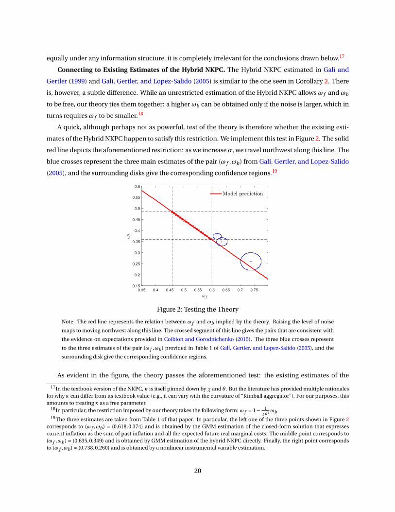
A quick, although perhaps not as powerful, test of the theory is therefore whether the existing esti-

mates of the Hybrid NKPC happen to satisfy this restriction. We implement this test in Figure 2. The solid

red line depicts the aforementioned restriction: as we increaseσ, we travel northwest along this line. The

blue crosses represent the three main estimates of the pair (ω f ,ωb) from Galí, Gertler, and Lopez-Salido

(2005), and the surrounding disks give the corresponding confidence regions.19

0.35 0.4 0.45 0.5 0.55 0.6 0.65 0.7 0.75

0.15

0.2

0.25

0.3

0.35

0.4

0.45

0.5

0.55

0.6

Figure 2: Testing the Theory

Note: The red line represents the relation between ω f and ωb implied by the theory. Raising the level of noise

maps to moving northwest along this line. The crossed segment of this line gives the pairs that are consistent with

the evidence on expectations provided in Coibion and Gorodnichenko (2015). The three blue crosses represent

to the three estimates of the pair (ω f ,ωb ) provided in Table 1 of Galí, Gertler, and Lopez-Salido (2005), and the

surrounding disk give the corresponding confidence regions.

As evident in the figure, the theory passes the aforementioned test: the existing estimates of the

17In the textbook version of the NKPC, κ is itself pinned down by χ and θ. But the literature has provided multiple rationalesfor why κ can differ from its textbook value (e.g., it can vary with the curvature of “Kimball aggregator”). For our purposes, thisamounts to treating κ as a free parameter.

18In particular, the restriction imposed by our theory takes the following form: ω f = 1− 1χρ2 ωb .

19The three estimates are taken from Table 1 of that paper. In particular, the left one of the three points shown in Figure 2corresponds to (ω f ,ωb ) = (0.618,0.374) and is obtained by the GMM estimation of the closed-form solution that expressescurrent inflation as the sum of past inflation and all the expected future real marginal costs. The middle point corresponds to(ω f ,ωb ) = (0.635,0.349) and is obtained by GMM estimation of the hybrid NKPC directly. Finally, the right point correspondsto (ω f ,ωb ) = (0.738,0.260) and is obtained by a nonlinear instrumental variable estimation.

20

Hybrid NKPC can be rationalized by some level of noise.20 But is the requisite level of noise empirically

plausible? We address this question next.

Bringing in the evidence on expectations. In Section 4.3, we discussed how CG have estimated a

key moment of the average forecasts, namely the coefficient KCG of regression (25), and how our results

provide a mapping from this moment to the pair (ω f ,ωb). We now use this mapping to translate the

confidence interval of KCG estimated in CG to a segment of the line in Figure 2.

In particular, we take CG’s baseline OLS regression, which appears as condition (11) of their paper

and concerns the one-year ahead average forecast of inflation in the Survey of Professional Forecasters.21

As reported in column (1) of Table 1 of that paper, this yields a mean estimate for KCG equal to 1.193,

with a standard deviation of 0.185. Translating the 95% confidence interval through the mapping seen in

Figure 1 earlier on yields the highlighted segment of the red line in Figure 2 here.

In short, this segment identifies the combinations of (ω f ,ωb) that can be rationalized with a level

of noise consistent with the expectation evidence in CG. Clearly, only the third of the three estimates

provided by Galí, Gertler, and Lopez-Salido (2005), that corresponding to the furthest right point in the

figure, is noticeably away from this segment. This happens to be the estimate that these authors trust

the least for independent, econometric, reasons.

We conclude that, when the theory is disciplined by the evidence in CG, it generates distortions

broadly in line with existing estimates of the Hybrid NKPC. Or, more succinctly, the informational fric-

tion implicit in the expectations data may alone account for all the observed inertia in inflation.

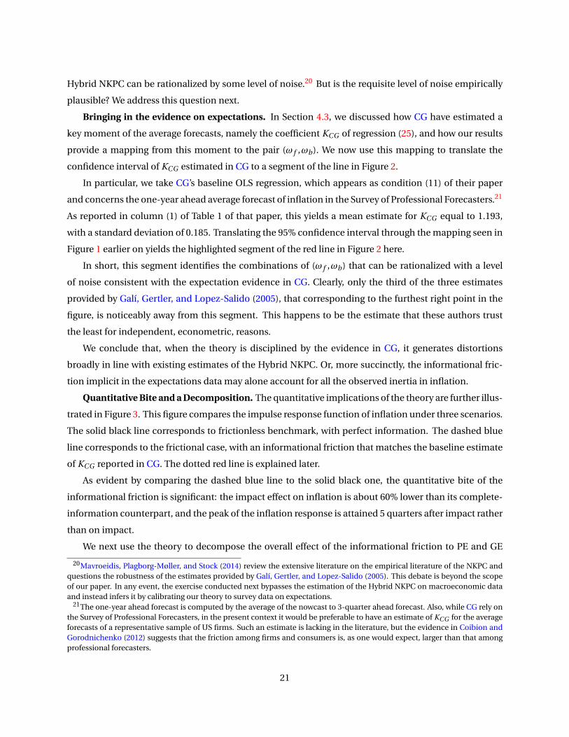
Quantitative Bite and a Decomposition. The quantitative implications of the theory are further illus-

trated in Figure 3. This figure compares the impulse response function of inflation under three scenarios.

The solid black line corresponds to frictionless benchmark, with perfect information. The dashed blue

line corresponds to the frictional case, with an informational friction that matches the baseline estimate

of KCG reported in CG. The dotted red line is explained later.

As evident by comparing the dashed blue line to the solid black one, the quantitative bite of the

informational friction is significant: the impact effect on inflation is about 60% lower than its complete-

information counterpart, and the peak of the inflation response is attained 5 quarters after impact rather

than on impact.

We next use the theory to decompose the overall effect of the informational friction to PE and GE

20Mavroeidis, Plagborg-Møller, and Stock (2014) review the extensive literature on the empirical literature of the NKPC andquestions the robustness of the estimates provided by Galí, Gertler, and Lopez-Salido (2005). This debate is beyond the scopeof our paper. In any event, the exercise conducted next bypasses the estimation of the Hybrid NKPC on macroeconomic dataand instead infers it by calibrating our theory to survey data on expectations.

21The one-year ahead forecast is computed by the average of the nowcast to 3-quarter ahead forecast. Also, while CG rely onthe Survey of Professional Forecasters, in the present context it would be preferable to have an estimate of KCG for the averageforecasts of a representative sample of US firms. Such an estimate is lacking in the literature, but the evidence in Coibion andGorodnichenko (2012) suggests that the friction among firms and consumers is, as one would expect, larger than that amongprofessional forecasters.

21

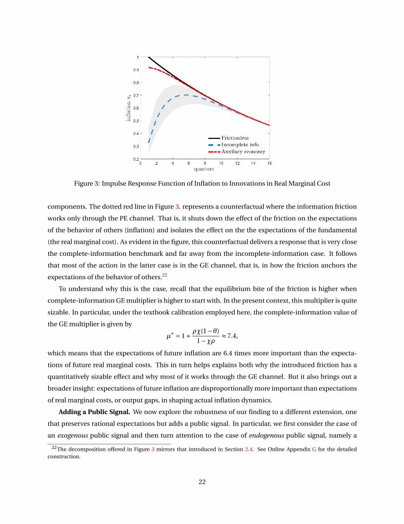
Figure 3: Impulse Response Function of Inflation to Innovations in Real Marginal Cost

components. The dotted red line in Figure 3. represents a counterfactual where the information friction

works only through the PE channel. That is, it shuts down the effect of the friction on the expectations

of the behavior of others (inflation) and isolates the effect on the the expectations of the fundamental

(the real marginal cost). As evident in the figure, this counterfactual delivers a response that is very close

the complete-information benchmark and far away from the incomplete-information case. It follows

that most of the action in the latter case is in the GE channel, that is, in how the friction anchors the

expectations of the behavior of others.22

To understand why this is the case, recall that the equilibrium bite of the friction is higher when

complete-information GE multiplier is higher to start with. In the present context, this multiplier is quite

sizable. In particular, under the textbook calibration employed here, the complete-information value of

the GE multiplier is given by

µ∗ = 1+ ρχ(1−θ)

1−χρ ≈ 7.4,

which means that the expectations of future inflation are 6.4 times more important than the expecta-

tions of future real marginal costs. This in turn helps explains both why the introduced friction has a

quantitatively sizable effect and why most of it works through the GE channel. But it also brings out a

broader insight: expectations of future inflation are disproportionally more important than expectations

of real marginal costs, or output gaps, in shaping actual inflation dynamics.

Adding a Public Signal. We now explore the robustness of our finding to a different extension, one

that preserves rational expectations but adds a public signal. In particular, we first consider the case of

an exogenous public signal and then turn attention to the case of endogenous public signal, namely a

22The decomposition offered in Figure 3 mirrors that introduced in Section 2.4. See Online Appendix G for the detailedconstruction.

22

noisy statistic of inflation. The first case affords an analytical characterization; the second case requires

a numerical approximation but, as shown here, leads to similar conclusions.23

Consider the first case, that is, let the firms also observe (and have common knowledge of) a pub-

lic signal of the form zt = ξt + εt , with εt ∼ N (0,ν2), in addition the private signals considered so far.

Appendix D contains a formal analysis of this case. Here, we briefly discuss the main insights and their

quantitative implications.

Ceteris paribus, the addition of public information reduces the documented distortions by increas-

ing the degree of common knowledge. But it also reduces the predictability of the average forecasts

errors. The relevant question is therefore how the accommodation of public information affects the pre-

ceding findings above under the requirement that the theory continues to match the available evidence

on expectations.

In our benchmark, the CG coefficient was identifying the value ofσ, which in turn was pinning down

the pair (ω f ,ωb), or equivalently the equilibrium dynamics. Now, the CG coefficient and the equilibrium

dynamics alike depend on two unknown parameters, the precisions τx ≡ σ−2 and τz ≡ ν−2 of, respec-

tively, the private and the public information. As a result, we loose point identification but preserve

set identification: only certain pairs of τz and τx are consistent, under the lens of the theory, with the

evidence in CG. Furthermore, because the theoretical value of KCG converges to zero as the public infor-

mation becomes sufficiently precise, the estimated value of KCG puts an upper bound on τz .24

Figure 4 illustrates the implications of these properties for the documented distortions. On the hori-

zontal axis, we let τz vary between zero (our benchmark) and the aforementioned bound. For each τz in

this range, we find the value of τx that matches the point estimate of KCG provided in CG and report the

implied values forω f andωb . The upper bound on τz turns out to be quite low, simply because evidence

in CG points towards high predictability in average forecast errors, which in turn requires a significant

departure from common knowledge. What is more, the distortions increase as we raise τz within the

admissible range. That is, once the theory is disciplined with the relevant evidence, the incorporation of

public information reinforces the documented distortions.

So far, we have focused the case in which the source of public information is exogenous. We now ex-

plore the case where this is endogenous. In particular, we let the public signal be zt =πt +νt , which can

be thought of as statistic of inflation contaminated with measurement error.25 Similar to the exogenous-

23We thank an anonymous referee for suggesting this exploration.24That is, the set of the admissible values for the pair (τx ,τz ) can be expressed as

S(KCG ) = {(τx ,τz ) : τz ≤ T (KCG ) and τx = f (τz ,KCG )

},

where KCG is the CG moment, T (·) is a function that gives corresponding upper bound on τz , and f (·) is a function that givesthe value of τx that lets the theory match this moment for any given τz below the aforementioned bound.

25This specification is close to that studied in Nimark (2008). The main difference is that the theory is herein disciplined bythe evidence in Coibion and Gorodnichenko (2015).

23

Figure 4: The Role of Public Information

information case, matching the Coibion-Gorodnichenko moment puts an upper bound on the infor-

mativeness of this signal. Different from the exogenous-information case, this informativeness is now

endogenous to the actual inflation dynamics. This introduces an additional fixed point problem, which

can only be solved numerically.

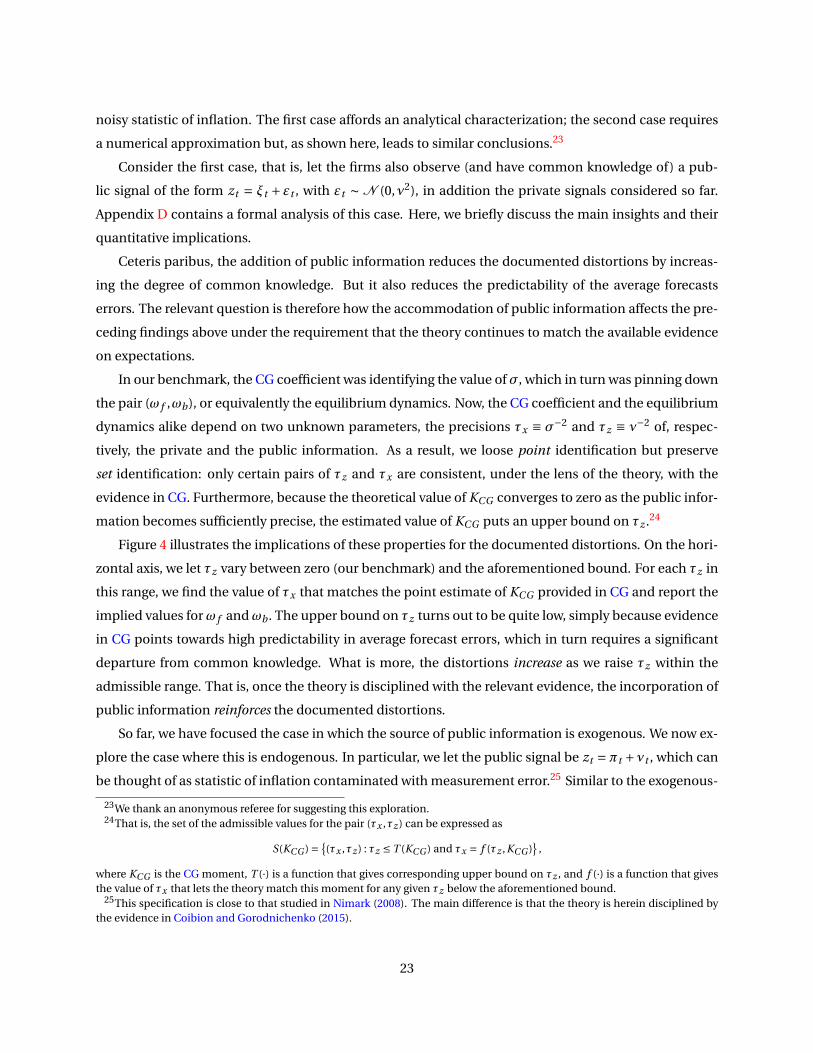
Figure 5: IRF of Inflation, Exogenous vs Endogenous Information

Figure 6 compares the IRF of inflation to real-marginal-cost innovations under three information

structures, all required to match the regression coefficient KCG estimated in CG. The blue, solid line

corresponds to our benchmark. The red, dashed line correspond to the case in which the public signal is

exogenous and its precision equals the aforementioned upper bound. The area between this line and the

benchmark one spans all the admissible parameterizations of the exogenous-information case. Finally,

24

the black, dotted line corresponds to the case in which the public signal is endogenous and its precision

equals the appropriate upper bound. The area between this line and the benchmark one spans all the

admissible parameterizations of the endogenous-information case.

The main takeaways are two. First, the exogenous-information setting provides a useful analytical

tool to understand the more realistic but less tractable endogenous-information case. Second, the ac-

commodation of public information, exogenous or endogenous, only reinforces the quantitative find-

ings once the theory is disciplined by the evidence on expectations in CG.

A third, subtler takeaway is that the endogenous public statistic appears to contribute to more per-

sistence than the exogenous public signal. We find this intriguing and we suspect it is because inflation

moves more sluggishly than the fundamental, thus slowing down the information diffusion. Nimark

(2008) also hypothesizes that endogenous signals add persistence. The logic is, however, complicated

by the fact that, as we vary the form of the signal, we adjust its precision to make sure that theory keeps

matching the CG moment.

Remarks. As emphasized at the end of Section 4.3, what enters either the CG coefficient or the actual

dynamics of inflation according to our theory is the perceived level of noise, not the actual one. It follows

that the employed method of identifying the friction and the obtained quantitative results are robust to

the possibility that agents are over-confident and overreact to private information. For the reasons al-

ready explained, this would not have been the case if we had used either the individual-level counterpart

of the CG coefficient or the cross-sectional dispersion of forecasts.

One may alternatively try to jointly match multiple moments of the average and individual forecasts

at once—or to consider an incomplete-information extension of the entire New Keynesian model and

estimate it with maximum likelihood on the basis of data on both outcomes and expectations. How

valuable this is depends, in part, on the questions of interest and, in part, on subjective judgements

about which approach is more transparent or less susceptible to model mis-specification. We hope that

the exercise conducted above offers a simple, useful, first pass. Complementary exercises, which tough

focus on different questions, are offered in Nimark (2014) and Melosi (2016).

6 Application to Dynamic IS

Now we turn to the effects of incomplete information on the aggregate demand. As already shown in

Corollary 3, through the lens of a perfect-information model, the Euler equation is modified as if there

is additional discounting together with habit persistence. In this section, we illustrate the quantitative

potential of this idea. We also build a bridge to the HANK literature by showing that the habit-like slug-

gishness generated by the informational friction is amplified when the agents with the highest MPC are

also the ones with the most cyclical income (Patterson, 2019; Flynn, Patterson, and Sturm, 2019).

25

A HANK-like extension. We consider a perpetual-youth, overlapping-generations version of the New

Keynesian model, along the lines of Piergallini (2007), Del Negro, Giannoni, and Patterson (2015), and

Farhi and Werning (2017). As in those papers, finite horizons (mortality risk) serve as convenient proxies

for liquidity constraints, self-control problems, and other micro-level friction that help explain why most

estimates of the MPC in microeconomic data are almost an order of magnitude large than that predicted

by the textbook, infinite-horizon model. We take this basic insight a step further by letting heterogeneity

in mortality risk capture heterogeneity in the MPC. We couple this with heterogeneity in cyclical expo-

sure. And, of course, we let information be incomplete.

Let us fill in the details. There are two types, or groups, of consumers, indexed by g ∈ {1,2}, with

respective massπg . In each period, a consumer in group g remains alive with probability$g ∈ (0,1]; with

the remaining probability, she dies and gets replaced by a new consumer of the same type. We allow the

households to trade a riskless bond, whose real return is denoted by Rt , and give them access to actuarily

fair annuities, so that the effective return to saving is Rt$g

conditional on survival and zero otherwise. We

nevertheless preclude them from trading more sophisticated assets, such as GDP futures, so that we can

bypass the complications of endogenous information aggregation. We also let firms profits be taxed by

the government and distributed in a lump sum manner to all consumers, regardless of age. We finally

allow the labor income of each group to have a differential exposure to the business cycle.

Consider a consumer i , of type g , born in period τ. Taking into account the mortality risk, her ex-

pected lifetime utility at birth is given by

∞∑t=τ

(χ$g

)t−τ log(Ci ,g ,t ;τ

),

where Ci ,g ,τ;t denotes her consumption in period t (conditional on survival) and β ∈ (0,1) is the subjec-

tive discount factor. Her budget constraint, on the other hand, is given by

Ci ,g ,τ;t +Si ,g ,τ;t+1 = Rt

$gSi ,g ,τ;t + (Yt )φg , ∀τ≥ t

where Si ,g ,t ;τ denotes savings in terms of the riskless bond, Yt denotes aggregate income, andφg param-

eterizes the elasticity of group g ’s income with respect to aggregate income.

We henceforth work with the log-linearized solution around a steady state in which there are no

shocks, χRt = 1, and Ct = Yt = Y ∗, where Y ∗ represents the natural rate of output.26 Using lower-case

variables to represent log-deviations from the steady state (e.g., rt ≡ logRt − logχ), we can express group

g ’s average consumption as follows:

cg ,t = (1−χ$g )∞∑

k=0(χ$g )kEt [φg yt+k ]−χ$g

∞∑k=0

(χ$g )kEt [rt+k ], g ∈ {1,2}, (27)

26To simplify the exposition, we suppress the production side of the economy and the determination of the flexible-price out-comes. The details can be filled in the usual way; let technology be linear in labor and assume constant aggregate productivityand constant monopoly power to get a time-invariant natural rate of output.

26

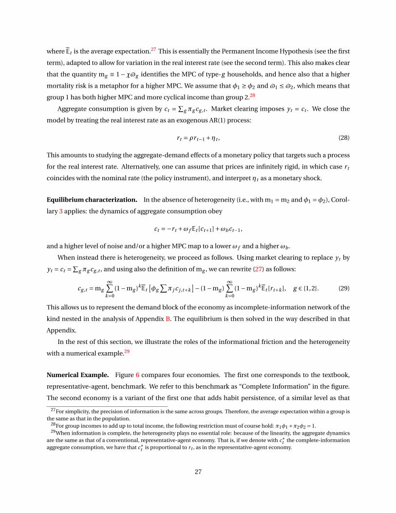
where Et is the average expectation.27 This is essentially the Permanent Income Hypothesis (see the first

term), adapted to allow for variation in the real interest rate (see the second term). This also makes clear

that the quantity mg ≡ 1−χ$g identifies the MPC of type-g households, and hence also that a higher

mortality risk is a metaphor for a higher MPC. We assume that φ1 ≥ φ2 and $1 ≤$2, which means that

group 1 has both higher MPC and more cyclical income than group 2.28

Aggregate consumption is given by ct = ∑g πg cg ,t . Market clearing imposes yt = ct . We close the

model by treating the real interest rate as an exogenous AR(1) process:

rt = ρrt−1 +ηt , (28)

This amounts to studying the aggregate-demand effects of a monetary policy that targets such a process

for the real interest rate. Alternatively, one can assume that prices are infinitely rigid, in which case rt

coincides with the nominal rate (the policy instrument), and interpret ηt as a monetary shock.

Equilibrium characterization. In the absence of heterogeneity (i.e., with m1 = m2 andφ1 =φ2), Corol-

lary 3 applies: the dynamics of aggregate consumption obey

ct =−rt +ω f Et [ct+1]+ωbct−1,

and a higher level of noise and/or a higher MPC map to a lower ω f and a higher ωb .

When instead there is heterogeneity, we proceed as follows. Using market clearing to replace yt by

yt = ct =∑g πg cg ,t , and using also the definition of mg , we can rewrite (27) as follows:

cg ,t = mg

∞∑k=0

(1−mg )kEt[φg

∑π j c j ,t+k

]− (1−mg )∞∑

k=0(1−mg )kEt [rt+k ], g ∈ {1,2}. (29)

This allows us to represent the demand block of the economy as incomplete-information network of the

kind nested in the analysis of Appendix B. The equilibrium is then solved in the way described in that

Appendix.

In the rest of this section, we illustrate the roles of the informational friction and the heterogeneity

with a numerical example.29

Numerical Example. Figure 6 compares four economies. The first one corresponds to the textbook,

representative-agent, benchmark. We refer to this benchmark as “Complete Information” in the figure.

The second economy is a variant of the first one that adds habit persistence, of a similar level as that

27For simplicity, the precision of information is the same across groups. Therefore, the average expectation within a group isthe same as that in the population.

28For group incomes to add up to total income, the following restriction must of course hold: π1φ1 +π2φ2 = 1.29When information is complete, the heterogeneity plays no essential role: because of the linearity, the aggregate dynamics

are the same as that of a conventional, representative-agent economy. That is, if we denote with c∗t the complete-informationaggregate consumption, we have that c∗t is proportional to rt , as in the representative-agent economy.

27

found in the DSGE literature.30 We refer to this economy as “Complete Info + Habit.” The remaining two

economies remove habit but add incomplete information. Both of them feature an average MPC equal to

m = .30, which is roughly consistent with the relevant evidence. The one referred to as “Incomplete Info”

in the figure, abstracts from heterogeneity; this is the economy described in Corollary 3. The other one,

which is referred to as “Incomplete Info + HANK” in the figure, adds heterogeneity; this is the network-

like economy described above and solved with the methods developed in Appendix B. In particular, this

economy features two groups of consumers, with the first group having both a higher MPC and a more

cyclical income: m1 = .55, m2 = .05, φ1 = 2, and φ2 = 0.

0 2 4 6 8 10 12 14 16

0.1

0.2

0.3

0.4

0.5

0.6

0.7

0.8

0.9

1

Figure 6: IRF of Consumption, Heterogeneous vs Homogeneous Agents

Let us first compare “Incomplete Info” to “Complete Info + Habit.” This extends the lesson of the

previous section from the inflation context to the consumption context: the informational friction alone

generates a similar degree of sluggishness as that generate by habit persistence in the DSGE literature.

Importantly, whereas the degree of habit assumed in that literature is far larger than that supported by

micro-economic evidence (Havranek, Rusnak, and Sokolova, 2017), the informational friction assumed

here is broadly consistent with survey evidence. This illustrates how our approach help merge the gap

between the micro and macro estimates of habit.

Relatedly, if we consider an extension with transitory idiosyncratic income shocks along the lines of

Appendix E, our economy can feature simultaneously a large and front-loaded response to such shocks

30In particular, we assume external habit and write the the representative consumer’s utility is given by log(Ct −bCt ), whereCt and Ct denote, respectively, own consumption and aggregate consumption. In equilibrium, Ct =Ct and the log-linearizedEuler condition reduces to the following low of motion of consumption:

ct =−1−b

1+brt + 1

1+bEt [ct+1]+ b

1+bct−1.

We finally set b = .7, which is in the middle of the macro-level estimates reported in the meta-analysis by Havranek, Rusnak,and Sokolova (2017).

28

at the micro level, in line with the relevant microeconomic evidence, and at the same time significant a

dampened and sluggish response to monetary policy at the macro level, in line with the relevant macroe-

conomic evidence. By contrast, if there was true habit persistence in consumption of the kind and level

assumed in the DSGE literature, the micro-level responses would have also be dampened and sluggish,

contradicting the relevant microeconomic evidence. This idea is pushed further in a recent paper by

Auclert, Rognlie, and Straub (2020).

Finally, let us inspect the economy “Incomplete Info + HANK.” Needless to say, this economy is not

meant to capture a realistic degree of heterogeneity: our two-group specification is only a gross ap-

proximation to the kind of heterogeneity captured in the quantitative HANK literature (e.g., Kaplan and

Violante, 2014; Kaplan, Moll, and Violante, 2016)). Nevertheless, this economy helps illustrate how such

heterogeneity, and in particular the kind of positive cross-sectional correlation between MPCs and in-

come cyclicality documented in Patterson (2019), can reinforce both the habit-like sluggishness and the

myopia-like dampening generated by incomplete information. We hope that this illustration will invite

more work on the intersection of the incomplete-information and HANK literatures.

7 Conclusion

We offered a toolbox for understanding and quantifying the macroeconomic effects of incomplete in-

formation, and higher-order uncertainty in particular. This toolbox relied on the use of appropriate,

simplifying assumptions. This precluded the analysis of certain issues, such as the endogeneity of the

information. But it afforded a high level of theoretical precision, a sharp comparison of incomplete in-

formation to bounded rationality, and a straightforward quantitative implementation.

An integral part of our contribution was the connection built to the available evidence on expecta-

tions. In particular, we highlighted why the combination of the evidence on the underreaction of the

average forecasts provided in Coibion and Gorodnichenko (2012, 2015) and that on the overreaction of

individual forecasts provided in Bordalo et al. (2018) and Kohlhas and Broer (2019) speaks in favor of

incomplete information over two alternatives, cognitive discounting and level-k thinking, that capture

a similar form of GE attention as higher-order uncertainty but abstract from dispersed information. We

further clarified why the first kind of evidence may be the most relevant for the quantification of the

documented distortions, at least within the class of models under consideration.

The usefulness of the provided tools was illustrated in the context of inflation. For this purpose,

we treated the real marginal cost as exogenous and we focused on how incomplete information works

through the NKPC alone. Future work may use the multi-variate extension of our results described in

Appendix B for more ambitious quantitative endeavors that require the incorporation of the two-way

interaction between the NKPC and the Dynamic IS curve.

Another direction for future work may be the extension of our results to more flexible departures

29

from rational expectations. For instance, the analysis can readily be extended to let agents have a mis-

specified prior not only about the precision of their information but also about the persistence of the

fundamental (and hence of the equilibrium outcome, too). When the perceived persistence is lower than

the actual one, this extension helps proxy for cognitive discounting as in Gabaix (2019). When the oppo-

site is true, it accommodates a form of over-extrapolative beliefs of a similar flavor as that in Greenwood

and Shleifer (2014) and Gennaioli, Ma, and Shleifer (2015). This or other similar extensions could help

develop a “unifying” framework, which in turn could be used to address a richer set of empirical regu-

larities and their macroeconomic implications—such as the question of whether average and individual

forecasts respond differentially to different shocks and how this matters for macroeconomic outcomes.

30

References

Abel, Andrew B. and Olivier J. Blanchard. 1983. “An Intertemporal Model of Saving and Investment.”

Econometrica 51 (3):675–692.

Allen, Franklin, Stephen Morris, and Hyun Song Shin. 2006. “Beauty Contests and Iterated Expectations

in Asset Markets.” Review of financial Studies 19 (3):719–752.

Alvarez, Fernando and Francesco Lippi. 2014. “Price Setting with Menu Cost for Multiproduct Firms.”

Econometrica 82 (1):89–135.

Angeletos, George-Marios and Chen Lian. 2016. “Incomplete Information in Macroeconomics: Accom-

modating Frictions in Coordination.” Handbook of Macroeconomics 2:1065–1240.

———. 2018. “Forward Guidance without Common Knowledge.” American Economic Review

108 (9):2477–2512.

Angeletos, George-Marios and Alessandro Pavan. 2007. “Efficient Use of Information and Social Value of

Information.” Econometrica 75 (4):1103–1142.

Auclert, Adrien, Matthew Rognlie, and Ludwig Straub. 2020. “Micro Jumps, Macro Humps: monetary

policy and business cycles in an estimated HANK model.” Mimeo .

Bachmann, Rüdiger, Ricardo J. Caballero, and Eduardo M. R. A. Engel. 2013. “Aggregate Implications of

Lumpy Investment: New Evidence and a DSGE Model.” American Economic Journal: Macroeconomics

5 (4):29–67.

Bergemann, Dirk, Tibor Heumann, and Stephen Morris. 2015. “Information and Volatility.” Journal of

Economic Theory 158:427–465.

Bergemann, Dirk and Stephen Morris. 2013. “Robust Predictions in Games with Incomplete Informa-

tion.” Econometrica 81 (4):1251–1308.

Bordalo, Pedro, Nicola Gennaioli, Yueran Ma, and Andrei Shleifer. 2018. “Over-reaction in Macroeco-

nomic Expectations.” NBER Working Paper No. 24932 .

Caballero, Ricardo J. and Eduardo M. R. A. Engel. 1999. “Explaining Investment Dynamics in U.S. Manu-

facturing: A Generalized (S, s) Approach.” Econometrica 67 (4):783–826.

Carroll, Christopher D., Edmund Crawley, Jiri Slacalek, Kiichi Tokuoka, and Matthew N. White. 2020.

“Sticky Expectations and Consumption Dynamics.” American Economic Journal: Macroeconomics

forthcoming.

31

Carvalho, Carlos, Stefano Eusepi, Emanuel Moench, and Bruce Preston. 2017. “Anchored Inflation Ex-

pectations.” .

Christiano, Lawrence J, Martin Eichenbaum, and Charles L Evans. 2005. “Nominal Rigidities and the

Dynamic Effects of a Shock to Monetary Policy.” Journal of Political Economy 113 (1):1–45.

Coibion, Olivier and Yuriy Gorodnichenko. 2012. “What Can Survey Forecasts Tell Us about Information

Rigidities?” Journal of Political Economy 120 (1):116–159.

———. 2015. “Information Rigidity and the Expectations Formation Process: A Simple Framework and

New Facts.” American Economic Review 105 (8):2644–78.

Del Negro, Marco, Marc P Giannoni, and Christina Patterson. 2015. “The Forward Guidance Puzzle.” FRB

of New York mimeo .

Evans, George W and Seppo Honkapohja. 2012. Learning and expectations in macroeconomics. Princeton

University Press.

Farhi, Emmanuel and Iván Werning. 2017. “Monetary Policy, Bounded Rationality, and Incomplete Mar-

kets.” NBER Working Paper No. 23281 .

———. 2019. “Monetary Policy, Bounded Rationality, and Incomplete Markets.” American Economic

Review forthcoming.

Flynn, Joel, Christina Patterson, and John Sturm. 2019. “Shock Propagation and the Fiscal Multiplier:

The Role of Heterogeneity.” MIT and Northwestern University mimeo .

Fuhrer, Jeff. 2012. “The Role of Expectations in Inflation Dynamics.” International Journal of Central

Banking .

Gabaix, Xavier. 2019. “A Behavioral New Keynesian Model.” Harvard mimeo .

Galí, Jordi. 2008. Monetary Policy, Inflation, and the Business Cycle: An Introduction to the New Keynesian

Framework and Its Applications Second edition. Princeton University Press.

Galí, Jordi and Mark Gertler. 1999. “Inflation dynamics: A structural econometric analysis.” Journal of

Monetary Economics 44 (2):195–222.

Galí, Jordi, Mark Gertler, and J David Lopez-Salido. 2005. “Robustness of the estimates of the hybrid New

Keynesian Phillips curve.” Journal of Monetary Economics 52 (6):1107–1118.

Gennaioli, Nicola, Yueran Ma, and Andrei Shleifer. 2015. “Expectations and investment.” In NBER

Macroeconomics Annual 2015, Volume 30. University of Chicago Press.

32

Golosov, Mikhail and Robert E Lucas Jr. 2007. “Menu Costs and Phillips Curves.” Journal of Political

Economy 115 (2):171–199.

Greenwood, Robin and Andrei Shleifer. 2014. “Expectations of returns and expected returns.” Review of

Financial Studies 27 (3):714–746.

Havranek, Tomas, Marek Rusnak, and Anna Sokolova. 2017. “Habit Formation in Consumption: A Meta-

Analysis.” European Economic Review 95:142–167.

Hayashi, Fumio. 1982. “Tobin’s Marginal q and Average q: A Neoclassical Interpretation.” Econometrica

50 (1):213–224.

Huo, Zhen and Marcelo Zouain Pedroni. 2019. “A Single-Judge Solution to Beauty Contests.” The Ameri-

can Economic Review forthcoming.

Huo, Zhen and Naoki Takayama. 2018. “Rational Expectations Models with Higher Order Beliefs.”

miméo, Yale University.

Jung, Jeeman and Robert J. Shiller. 2005. “Samuelson’s Dictum and the Stock Market.” Economic Inquiry

43 (2):221–228.

Kaplan, Greg, Benjamin Moll, and Giovanni L Violante. 2016. “Monetary Policy According to HANK.”

NBER Working Paper No. 21897 .

Kaplan, Greg and Giovanni L. Violante. 2014. “A Model of the Consumption Response to Fiscal Stimulus

Payments.” Econometrica 82 (4):1199–1239.

Kasa, Kenneth, Todd B. Walker, and Charles H. Whiteman. 2014. “Heterogeneous Beliefs and Tests of

Present Value Models.” The Review of Economic Studies 81 (3):1137–1163.

Khan, Aubhik and Julia K. Thomas. 2008. “Idiosyncratic Shocks and the Role of Nonconvexities in Plant

and Aggregate Investment Dynamics.” Econometrica 76 (2):395–436.

Kiley, Michael T. 2007. “A Quantitative Comparison of Sticky-Price and Sticky-Information Models of

Price Setting.” Journal of Money, Credit and Banking 39 (s1):101–125.

Kohlhas, Alexandre and Tobias Broer. 2019. “Forecaster (Mis-)Behavior.” IIES miméo .

Lucas, Robert E. Jr. 1972. “Expectations and the Neutrality of Money.” Journal of Economic Theory

4 (2):103–124.

———. 1976. “Econometric Policy Evaluation: A Critique.” Carnegie-Rochester Conference Series on Pub-

lic Policy 1:19 – 46.

33

Mackowiak, Bartosz and Mirko Wiederholt. 2009. “Optimal Sticky Prices under Rational Inattention.”

American Economic Review 99 (3):769–803.

Mankiw, N. Gregory and Ricardo Reis. 2002. “Sticky Information versus Sticky Prices: A Proposal to

Replace the New Keynesian Phillips Curve.” Quarterly Journal of Economics 117 (4):1295–1328.

Marcet, Albert and Juan P Nicolini. 2003. “Recurrent hyperinflations and learning.” American Economic

Review 93 (5):1476–1498.

Matejka, Filip. 2016. “Rationally Inattentive Seller: Sales and Discrete Pricing.” Review of Economic

Studies 83 (3):1125–1155.

Mavroeidis, Sophocles, Mikkel Plagborg-Møller, and James H Stock. 2014. “Empirical evidence on infla-

tion expectations in the New Keynesian Phillips Curve.” Journal of Economic Literature 52 (1):124–88.

Melosi, Leonardo. 2016. “Signalling effects of monetary policy.” The Review of Economic Studies

84 (2):853–884.

Midrigan, Virgiliu. 2011. “Menu Costs, Multiproduct Firms, and Aggregate Fluctuations.” Econometrica

79 (4):1139–1180.

Morris, Stephen and Hyun Song Shin. 1998. “Unique Equilibrium in a Model of Self-fulfilling Currency

Attacks.” American Economic Review :587–597.

———. 2002. “Social Value of Public Information.” American Economic Review 92 (5):1521–1534.

———. 2006. “Inertia of Forward-looking Expectations.” The American Economic Review :152–157.

Nakamura, Emi and Jón Steinsson. 2013. “Price Rigidity: Microeconomic Evidence and Macroeconomic

Implications.” Annual Review of Economics 5 (1):133–163.

Nimark, Kristoffer. 2008. “Dynamic Pricing and Imperfect Common Knowledge.” Journal of Monetary

Economics 55 (2):365–382.

———. 2017. “Dynamic Higher Order Expectations.” Cornell Univeristy mimeo .

Nimark, Kristoffer, Ryan Chahrour, and Stefan Pitschner. 2019. “Sectoral Media Focus and Aggregate

Fluctuations.” mimeo .

Nimark, Kristoffer P. 2014. “Man-Bites-Dog Business Cycles.” American Economic Review 104 (8):2320–

67.

Patterson, Christina. 2019. “The Matching Multiplier and the Amplification of Recessions.” Northwestern

University mimeo .

34

Piergallini, Alessandro. 2007. “Real Balance Effects and Monetary Policy.” Economic Inquiry 44 (3):497–

511.

Reis, Ricardo. 2006. “Inattentive producers.” The Review of Economic Studies 73 (3):793–821.

Sargent, Thomas J. 1993. Bounded rationality in macroeconomics. Oxford University Press.

Sims, Christopher A. 2003. “Implications of Rational Inattention.” Journal of Monetary Economics

50 (3):665–690.

Singleton, Kenneth J. 1987. “Asset Prices in a Time-series Model with Disparately Informed, Competitive

Traders.” In New Approaches to Monetary Economics, edited by William A. Barnett and Kenneth J.

Singleton. Cambridge University Press, 249–272.

Smets, Frank and Rafael Wouters. 2007. “Shocks and Frictions in US Business Cycles: A Bayesian DSGE

Approach.” American Economic Review 97 (3):586–606.

Tirole, Jean. 2015. “Cognitive Games and Cognitive Traps.” Toulouse School of Economicss mimeo .

Vives, Xavier and Liyan Yang. 2017. “Costly Interpretation of Asset Prices.” mimeo, IESE/University of

Toronto.

Whittle, Peter. 1963. “Prediction and Regulation by Linear Least-Square Methods.” .

Woodford, Michael. 2003. “Imperfect Common Knowledge and the Effects of Monetary Policy.” Knowl-

edge, Information, and Expectations in Modern Macroeconomics: In Honor of Edmund S. Phelps .

Zorn, Peter. 2018. “Investment under Rational Inattention: Evidence from US Sectoral Data.” miméo,

University of Munich.

35

APPENDICES

A Proofs of Propositions in Main Text

This appendix contains the proofs of the results stated in the main text. The proofs of the auxiliary results

that appear in the various appendices are collected in Online Appendix K.

Proof of Proposition 1. Follows directly from the analysis in the main text.

Proof of Proposition 2. As a preliminary step, we look for the fundamental representation of the signals.

Define τη = σ−2η and τu = σ−2 as the reciprocals of the variances of, respectively, the innovation in the

fundamental and the noise in the signal. (In the main text, we have normalized ση = 1.) The signal

process can be rewritten as

xi ,t = M(L)

ηt

ui ,t

, with M(L) =[τ− 1

2η

11−ρL τ

− 12

u

].

Let B(L) denote the fundamental representation of the signal process. By definition, B(L) needs to be an

invertible process and it needs to satisfy the following requirement

B(L)B(L−1) = M(L)M′(L−1) =τ−1η +τ−1

u (1−ρL)(L−ρ)

(1−ρL)(L−ρ), (30)

which leads to

B(L) = τ−12

u

√ρ

λ

1−λL

1−ρL,

where λ is the inside root of the numerator in equation (30)

λ = 1

2

[ρ+ 1

ρ

(1+ τu

τη

)−

√(ρ+ 1

ρ

(1+ τu

τη

))2

−4

].

The forecast of a random variable

ft = A(L)

ηt

ui ,t

can be obtained by using the Wiener-Hopf prediction formula:31

Ei ,t [ ft ] = [A(L)M′(L−1)B(L−1)−1]

+ B(L)−1xi ,t .

Now we proceed to solve the equilibrium. Denote the agent’s equilibrium policy function as

ai ,t = h(L)xi ,t

31See Whittle (1963) for more details about Wiener-Hopf prediction formula.

36

for some lag polynomial h(L). The aggregate outcome can then be expressed as follows:

at = h(L)ξt = h(L)

1−ρLηt .

In the sequel, we verify that the above guess is correct and characterize h(L).

Consider the forecast of the fundamental. Note that

ξt =[τ− 1

2η

11−ρL 0

] ηt

ui ,t

,

from which it follows that

Ei ,t [ξt ] =G1(L)xi ,t , G1(L) ≡ λ

ρ

τu

τη

1

1−ρλ1

1−λL.

Consider the forecast of the future own and average actions. Using the guess that ai t+1 = h(L)xi ,t+1 and

at+1 = h(L)ξt+1, we have

at+1 =[τ− 1

2η

h(L)L(1−ρL) 0

] ηt

ui ,t

, ai ,t+1 −at+1 =[

0 τ− 1

2u h(L)

] ηt

ui ,t

,

and the forecasts are

Ei ,t [at+1] =G2(L)xi ,t , G2(L) ≡ λ

ρ

τu

τη

(h(L)

(1−λL)(L−λ)− h(λ)(1−ρL)

(1−ρλ)(L−λ)(1−λL)

),

Ei ,t[ai ,t+1 −at+1

]=G3(L)xi ,t , G3(L) ≡ λ

ρ

(h(L)(L−ρ)

L(L−λ)− h(λ)(λ−ρ)

λ(L−λ)− ρ

λ

h(0)

L

)1−ρL

1−λL

Now, turn to the fixed point problem that characterizes the equilibrium:

ai ,t = Ei ,t [ϕξt +βai ,t+1 +γat+1]

Using our guess, we can replace the left-hand side with h(L)xi ,t . Using the results derived above, on the

other hand, we can replace the right-hand side with[G1(L)+ (β+γ)G2(L)+βG3(L)

]xi ,t . It follows that

our guess is correct if and only if

h(L) =G1(L)+ (β+γ)G2(L)+βG3(L)

Equivalently, we need to find an analytic function h(z) that solves

h(z) =ϕλρ

τu

τη

1

1−ρλ1

1−λz+

+ (β+γ)λ

ρ

τu

τη

(h(z)

(1−λz)(z −λ)− h(λ)(1−ρz)

(1−ρλ)(z −λ)(1−λz)

)+βλ

ρ

(h(z)(z −ρ)

z(z −λ)− h(λ)(λ−ρ)

λ(z −λ)− ρ

λ

h(0)

z

)1−ρz

1−λz,

37

which can be transformed as

C (z)h(z) = d(z;h(λ),h(0))

where

C (z) ≡ z(1−λz)(z −λ)− λ

ρ

{β(z −ρ)(1−ρz)+ (β+γ)

τu

τηz

}d(z;h(λ),h(0)) ≡ϕλ

ρ

τu

τη

1

1−ρλ z(z −λ)− 1

ρ

(τu

τη

λ(β+γ)

1−ρλ +β(λ−ρ)

)z(1−ρz)h(λ)

−β(z −λ)(1−ρz)h(0)

Note that C (z) is a cubic equation and therefore contains with three roots. We will verify later that there

are two inside roots and one outside root. To make sure that h(z) is an analytic function, we choose h(0)

and h(λ) so that the two roots of d(z;h(λ),h(0)) are the same as the two inside roots of C (z). This pins

down the constants {h(0),h(λ)}, and therefore the policy function h(L)

h(L) =(1− ϑ

ρ

)ϕ

1−ρδ1

1−ϑL,

where ϑ−1 is the root of C (z) outside the unit circle.

Now we verify that C (z) has two inside roots and one outside root. C (z) can be rewritten as

C (z) =λ{− z3 +

(ρ+ 1

ρ+ 1

ρ

τu

τη+β

)z2 −

(1+β

(ρ+ 1

ρ

)+ β+γ

ρ

τu

τη

)z +β

}.

With the assumption that β > 0, γ > 0, and β+γ < 1, it is straightforward to verify that the following

properties hold:

C (0) =β> 0

C (λ) =−λγ 1

ρ

τu

τη< 0

C (1) = τu(1−β−γ)

τηρ+ (1−β)

(1

ρ+ρ−2

)> 0

Therefore, the three roots are all real, two of them are between 0 and 1, and the third one ϑ−1 is larger

than 1.

Finally, to show that ϑ is less than ρ, it is sufficient to show that

C

(1

ρ

)= τu(1−ρβ−ργ)

τηρ3 > 0.

Since C (ϑ−1) = 0, it has to be that ϑ−1 is larger than ρ−1, or ϑ< ρ.

38

Proof of Proposition 3. The equilibrium outcome in the hybrid economy is given by the following AR(2)

process:

at = ζ0

1−ζ1Lξt

where

ζ1 = 1

2ω f δ

(1−

√1−4δω f ωb

)and ζ0 = ϕζ1

ωb −ρω f δζ1(31)

and δ≡β+γ. The solution to the incomplete-information economy is

at =(1− ϑ

ρ

)(ϕ

1−ρδ)(

1

1−ϑLξt

),

To match the hybrid model, we need

ζ1 =ϑ and ζ0 =(1− ϑ

ρ

)ϕ

1−ρδ . (32)

Combining (31) and (32), and solving for the coefficients of ω f and ωb , we infer that the two economies

generate the same dynamics if and only if the following two conditions hold:

ω f =δρ2 −ϑδ(ρ2 −ϑ2)

(33)

ωb = ϑ(1−δϑ)ρ2

ρ2 −ϑ2 (34)

Since δ≡β+γ and since ϑ is a function of the primitive parameters (σ,ρ,β,γ), the above two conditions

give the coefficients ω f and ωb as as functions of the primitive parameters, too.

It is immediate to check that ω f < 1 and ωb > 0 if ϑ ∈ (0,ρ), which in turn is necessarily true for any

σ> 0; and that ω f = 1 and ωb = 0 if ϑ= ρ, which in turn is the case if and only if σ= 0. The proof of the

comparative statics in terms of σ is contained in the proof of Proposition 5.

Proof of Proposition 4 and 5. We first show that ω f is decreasing in ϑ and ωb is increasing in ϑ. This

can be verified as follows

∂ω f

∂ϑ= −δ(ρ2 +ϑ2)+2δ2ρ2ϑ

(δ(ρ2 −ϑ2))2 < −δ(ρ2 +ϑ)+2δρϑ

(δ(ρ2 −ϑ2))2 = −δ(ρ−ϑ)2

(δ(ρ2 −ϑ2))2 < 0

∂ωb

∂ϑ= ρ2(ρ2 +ϑ2 −2δϑρ2)

(ρ2 −ϑ2)2 > ρ2(ρ2 +ϑ2 −2ϑρ)

(ρ2 −ϑ2)2 =(

ρ

ρ+ϑ)2

> 0

Now it is sufficient to show that ϑ is increasing in γ. Note that

C

(1

ρ

)= τu(1−ρβ−ργ)

τηρ3 > 0 and C

(1

λ

)=−τu

τη

γβ

ρλ2 < 0

By the continuity of C (z), it must be the case that C (z) admits a root between 1ρ and 1

λ . Recall from the

proof of Proposition 2, ϑ−1 is the only outside root, and it follows that λ<ϑ< ρ. It also implies that C (z)

is decreasing in z in the neighborhood of z = ϑ−1, a property that we use in the sequel to characterize

39

comparative statics of ϑ.

Next, using the definition of C (z), namely

C (z) ≡−z3 +(ρ+ 1

ρ+ 1

ρ

τu

τη+β

)z2 −

(1+β

(ρ+ 1

ρ

)+ β+γ

ρ

τu

τη

)z +β,

taking its derivative with respect to γ, and evaluating that derivative at z =ϑ−1, we get

∂C (ϑ−1)

∂γ=− τu

ρτη< 0

Combining this with the earlier observation that ∂C (ϑ−1)∂z < 0, and using the Implicit Function Theorem,

we infer that ϑ is an increasing function of γ.

Similarly, taking derivative with respect to τu , we have

∂C (ϑ−1)

∂τu= 1

ρτηϑ−1(ϑ−1 −β−γ) > 1

ρτηϑ−1(1−β−γ) > 0.

Since τu =σ−2, we conclude that ϑ is also increasing in σ.

Proof of Proposition 6. With complete information, the PE component is given by

ϕ∞∑τ=0

βτEt [ξt+τ] = ϕ

1−ρβξt ,

and the GE component by

γ∞∑τ=0

βτEt [at+τ+1] = γ∞∑τ=0

βτEt

[ϕ

1−ρδξt+1

]= ργ

1−ρδϕ

1−ρβξt ,

from which part (i) is immediate.

Thus consider part (ii), namely the case with incomplete information. The aggregate outcome is

at = ϕ

1−ρδ(1− ϑ

ρ

)1

(1−ρL)(1−ϑL)ηt ≡ ϕ

1−ρδ(1− ϑ

ρ

) ∞∑τ=0

gτηt−τ

The PE component is given by

PEt = ϕ

1−ρβ(1− λ

ρ

)1

(1−ρL)(1−λL)ηt ≡ ϕ

1−ρβ(1− λ

ρ

) ∞∑τ=0

fτηt−τ

The sequence of gτ and fτ are given by

gτ = ρτ+1 −ϑτ+1

ρ−ϑ , and fτ = ρτ+1 −λτ+1

ρ−λ .

The GE multiplier µτ is given by

µτ =ϕ

1−ρδ(1− ϑ

ρ

)ϕ

1−ρβ(1− λ

ρ

) gτfτ

=(1+ ργ

1−ρδ)ρ−ϑρ−λ

gτfτ

=(1+ ργ

1−ρδ)ρτ+1 −ϑτ+1

ρτ+1 −λτ+1 .

40

With complete information, ϑ = λ = 0, gτ = fτ = ρτ, and we are back to part (i). With incomplete infor-

mation, we have ρ > ϑ> λ. To show µτ is increasing in τ, it is equivalent to show that gτfτ

is increasing in

τ. For τ= 0, g0 = f0 = 1, and g0

f0= 1. For τ= 1, g1 = ρ+ϑ and f1 = ρ+λ, and it follows that

g1

f1= ρ+ϑρ+λ > ρ+λ

ρ+λ = 1 = g0

f0.

For τ> 1, gτ = ρgτ−1 +ϑτ and fτ = ρ fτ−1 +λτ. To show

gτfτ

= ρgτ−1 +ϑτρ fτ−1 +λτ

> gτ−1

fτ−1,

it is equivalently to show

ϑτ fτ−1 >λτgτ−1

We prove this by induction. Suppose ϑτ fτ−1 >λτgτ−1 is true, then

ϑτ+1 fτ =ϑτ+1(ρ fτ−1 +λτ) >ϑ(ρλτgτ−1 +λτϑτ) = ρϑλτgτ−1 +λτϑτ+1

> ρλτ+1gτ−1 +λτ+1ϑτ =λτ+1(ρgτ−1 +ϑτ) =λτ+1gτ,

which completes the induction.

Finally, in the limit as τ goes to ∞,

limτ→∞

gτλτ

= limτ→∞

ρ−λρ−ϑ

ρτ+1 −ϑτ+1

ρτ+1 −λτ+1 = ρ−λρ−ϑ .

Therefore,

limτ→∞µτ =µ

∗.

Proof of Proposition 7. The proof follows directly from the discussion in Online Appendix C and Propo-

sition 10 therein.

B Multivariate Systems

Corollaries 2 and 3 require that each block of the New Keynesian model—the NKPC and the Dynamic IS

curve—is treated in isolation of the other. This is fine for certain purposes, including the exercise con-

ducted in Section 5. As another example, consider the question of how aggregate demand responds to

monetary policy. A version of this question can be addressed by assuming that monetary policy induces

an AR(1) path for the real interest rate and by studying the mapping from that path to the equilibrium

path of aggregate consumption. Corollary 3 then sheds light on how this mapping is distorted by the

assumed friction.

For other purposes, however, it is best to allow the “fundamental” in the one block of the model (e.g.,

the real interest rate faced by the consumers) to depend on the outcome of the other block (e.g., the

41

inflation generated by the joint behavior of the firms). How does this extra layer of GE feedback matters

for our main insights and the tractability of our solution?

We address this question by working out a multi-variate extension of our framework. The economy

consists of n groups, each containing a continuum of agents. Groups are indexed by g ∈ {1, ...,n}, agents

by (i , g ) where i ∈ [0,1] is an agent’s name and g her group affiliation (e.g., consumer or firm). The best

response of agent i in group g is specified as follows:32

ai ,g ,t =ϕgEi ,g ,t [ξt ]+βgEi ,g ,t [ai ,g ,t+1]+n∑

j=0γg jEi ,g ,t [a j ,t+1]. (35)

The parameters {βg } and {γg j } help parameterize, once again, PE and GE considerations. The main

novelty (and added complexity) is that GE effects now run, not only within groups, but also across groups.

This may correspond to the interaction of the two blocks of the New Keynesian model, or more abstractly

to a network structure across arbitrary groups of agents. Finally, the parameter ϕg captures the direct

exposure of group g to the exogenous shock.33

Turning now to the information structure, this is specified as a collection of private Gaussian signals,

one per agent and per period. In particular, the period-t signal received by agent i in group t is given by

xi ,g ,t = ξt +ui ,g ,t , ui ,g ,t ∼N (0,σ2g ). (36)

whereσg ≥ 0 parameterizes the noise of group g . Notice that, by allowingσg to differ g , we accommodate

rich information heterogeneity. For instance, firms could be more informed than consumers on average,

and “sophisticated” consumers could be more informed than “unsophisticated” ones.

Let at = (ag ,t ) be a column vector collecting the aggregate actions of all the groups (e.g., the vector of

aggregate consumption and aggregate inflation). Let ϕ = (ϕg ) be a column vector containing the value

of ϕg across the groups. Let β = diag{βg

}be a n ×n diagonal matrix whose off-diagonal elements are

zero and whose diagonal elements are the values of βg across groups. Finally, let γ = (γg k ) be an n ×n

matrix collecting the interaction parameters, γg j , and let δ≡β+γ. Similarly to Section 2, we impose that

βg ∈ (0,1) and the spectral radius of (I−β)−1γ is less than 1. The following extensions of Propositions 2

and 3 are then possible.

Proposition 8. There exists a unique equilibrium, and the aggregate outcome ag ,t of each group g is given

32Like our baseline framework, the extension considered here rules out the dependence of an agent’s best response on theconcurrent choices of others. This, however, is without serious loss of generality for two reasons. First, in all applications ofinterest, this dependence vanishes as the length of the time period goes to zero. Second, if we incorporate a general form ofsuch dependence by adding the term

∑j αg ,iEi , j ,t [ai , j ,t ] in equation (35), the results stated below, namely Propositions 8 and

9, continue to hold, modulo a minor adjustment in the cubic that appears in condition (37).33The parameter ϕg is allowed to be zero for some, but not all, g . For instance, if ξt represents an aggregate discount-factor

shock, it shows up in the Dynamic IS curve but not in NKPC. (And the converse is true of for a markup shock.)

42

by

ag ,t =n∑

j=1ψg , j

1− ϑ j

ρ

1−ϑ j Lξt

(37)

where {ψg , j } are fixed scalars, characterized in the Appendix A, and {ϑg } are the inverse of the outside roots

of the following polynomial:

C (z) = det

((δ−γ− Iz) diag

{z2 −

(ρ+ 1

ρ+ 1

ρσ2g

)z +1

}− z diag

{ 1

ρσ2g

}γ

). (38)

Proposition 9. There exist matrices ω f and ωb such that the incomplete-information economy is obser-

vationally equivalent to the following complete-information economy:

at =ϕξt +ω f δEt [at+1]+ωb at−1 (39)

The proofs of these results are presented at the end of this appendix. One subtlety with the represen-

tation offered in condition (39) is that this representation is no more unique: there are multiple values of

the matricesω f andωb that replicate the incomplete-information equilibrium. Intuitively, it is possible

to make agents myopic vis-a-vis the future by letting them discount enough either only their own group’s

future outcome, or the future outcomes of others groups too.34 This complicates the interpretation and

the comparative statics of the provided representation but is of little substantial consequence: although

the representation in terms of condition (39) is not unique, the equilibrium itself is determinate, and so

are its observable properties, which can be directly obtained from Proposition 8.

Proposition 8 is indeed quite telling. It shows that the equilibrium outcome can now be expressed as

a linear combination of n terms, each of which is an AR(2) process that has a similar structure as in our

baseline analysis. The one root of these processes is the same across g and is given, naturally, by that of

the fundamental. The other root, denoted above by ϑg , encodes how the information friction faced by

group g interacts with the network structure of the economy.

In the knife-edge case in which γ is diagonal, meaning that the behavior of each group is indepen-

dent of that of other groups, each ϑg is pinned down by the characteristics of group g alone and the

outcome of that group is given by the corresponding AR(2) process alone (ψg , j = 0 for j 6= g ). For generic

γ, instead, all the {ϑg } have to be jointly determined, and in addition, the outcome of a group depends

on all the n different AR(2) processes.

This reflects the rich network structure, or the rich cross-equation feedbacks, allowed by the present

extension. To appreciate this, consider the special case in whichβ= 0 andσg =σ for all g . In this case, we

show in Appendix A that the polynomial given in condition (38) reduces to the product of n quadratics,

34Indeed, both of the following two choices are possible: letω f have unit off-diagonal elements, meaning that a distortion isapplied only to expectations of own-group future outcomes; or let the elements of each row of ω f be the same, meaning thatthe same distortion is applied to all expectations. Once one of these choices is made, there is no residual indeterminacy.

43

one for each ϑg . Furthermore, the solution for each ϑg is in the same manner as in our baseline analysis,

with the g -th eigenvalue of the matrix γ in place of the scalar γ. Because the eigenvalues of γ encode the

GE feedback both within and across groups, we have that an increase in either kind of feedback maps to

a higher ϑg and, thereby, to both less amplitude and more volatility. The essence of our baseline analysis

is thus fully preserved.

To conclude, the results presented above offer, not only an illustration of the robustness of our main

insights to multi-variate systems, but also a straightforward numerical algorithm: one only needs to solve

the polynomial seen in condition (38). Contrast this with the complexity of the underlying higher-order

beliefs, which now entails not only the issue discussed in Section 2.4 but also the network structure of

the higher-order beliefs that each group holds about other groups. Proposition 2 may therefore prove

useful for future quantitative endeavors.35

As mentioned in the main text, the results developed here could assist the study and quantification

of incomplete-information versions, not only of the full New Keynesian model, but also of multi-sector

models or networks (Bergemann, Heumann, and Morris, 2015; Nimark, Chahrour, and Pitschner, 2019).

C Overconfidence

Consider an extension that lets agents mis-perceive the precision of their information, or equivalently

the level (standard deviation) of the noise in their signals: whereas the true level is σ, agents perceive it

to be σ, for some σ 6=σ. Over-confidence corresponds to σ<σ, under-confidence to σ>σ.

In a simple context, which abstracts from the fixed-point relation between outcomes and forecasts

and amounts to letting at = ξt , Kohlhas and Broer (2019) show that the individual-level counterpart of

the CG regression (25) yields a coefficient whose sign is the same as that of the difference between σ

and σ. The basic logic is this. When σ = σ, expectations are rational, so individual forecast errors are

orthogonal to own past revisions. When instead σ < σ, agents over-react to their current information

because they over-estimate its precision, so a positive forecast revision today tends to predict a negative

forecast error in the future. (And the converse is true if σ>σ.)

This logic extends to our context. But the key question of interest to us is how the accommodation

of over-confidence influences the fixed-point relation between outcomes and forecasts. The answer is

provided by the next result.

Proposition 10. (i) Propositions 2, 3, 4, 5 and 6 remain valid, modulo the replacement of σ with σ

throughout.

35Like our baseline result, this result depends on abstracting from the endogeneity of information. But unless the analyst isinterested per se in the effects of a particular endogeneity, this abstraction seems a cost worth paying given the great gain intractability. Furthermore, the exercise considered in the end of Section 5 indicates our results may offer a useful approximationto settings with endogenous signals as well.

44

(ii) Any moment of the average forecasts, including the coefficient KCG , is given by the same function

as in our baseline model, modulo the replacement of σ with σ.

Apart from establishing the robustness of all our formal results to over-confidence, this result un-

derscores that the documented distortions and their empirical footprint on, say, inflation and average

forecasts thereof depends only on the agents’ perception of the informational friction, not the actual

level of noise. The logic is the one articulated in the main text.

Suppose, now, that the analyst knows all parameters except σ and σ and wishes to quantify the equi-

librium effects of the friction under consideration (as we do, for example, in Section 5). Suppose further

that the analyst combines the CG coefficient with the individual-level counterpart estimated in Bordalo

et al. (2018) and Kohlhas and Broer (2019). Then, the CG coefficient alone allows the identification of σ

and the quantification of its effect on the actual dynamics. The individual-level counterpart allows the

identification of σ, but this does not affect the aforementioned quantitative evaluation.

A similar point applies if we replace in this argument the CG coefficient with any other moment of

the average forecasts, such as the persistence of the average forecast errors documented in Coibion and

Gorodnichenko (2012), and the moments estimated in Bordalo et al. (2018) and Kohlhas and Broer (2019)

with any other moment of the individual forecasts, such as the cross-sectional dispersion of the average

forecast errors. In this sense, any individual-level evidence drops out of the picture.

Of course, this is not a panacea. The bypassing of the individual-level evidence is justified for our

purposes because of a sufficiently narrow focus: we only care about the “macro picture” of how the mea-

sured sluggishness in average forecasts maps to myopia and anchoring in aggregate outcomes. But such

a bypassing may not be justified if one wishes to have a complete structural model of the joint determi-

nation of outcomes and forecasts at both the aggregate and the individual level. In this case, one could

use the tools developed here to jointly identify σ and σ from the combination of all the aforementioned

evidence. One could then also ask whether the simple model we have described so far could match a

multitude of moments of the individual and the average forecasts, or whether further enrichments are

needed, such as the distinction between “absolute” and “relative” confidence proposed in Kohlhas and

Broer (2019).

We leave these ideas, and a more careful exploration of the expectations data, for future work. In

this paper, we instead focus on how the toolbox we have developed here helps quantify the macro-level

distortions of interest, and on the importance played by GE feedbacks.

45

ONLINE APPENDICES

D Public Signals

Throughout the main analysis, we have assumed that the noise is entirely idiosyncratic. We have thus as-

sumed away, not only correlated errors in expectations, but also the coordination afforded when agents

condition their behavior on noisy but public information (Morris and Shin, 2002). In this appendix, we

accommodate these possibilities by letting agents observe, in addition to the private signal xi ,t = ξt +ui ,t

considered so far, a public signal of the form

zt = ξt +εt , (40)

where ui ,t ∼N (0,σ2u) and εt ∼N (0,σ2

ε) are, respectively, idiosyncratic and aggregate noises. We next let

σ−2 ≡ σ−2u +σ−2

ε measure the overall precision of the available information about the fundamental and

χ≡ σ−2ε

σ−2u +σ−2

εthe fraction of it that reflects public information, or common knowledge.36

Proposition 11. In the extension with public signals described above, the following properties are true.

(i) The equilibrium outcome is given by

at = aξt + vt ,

where aξt is the projection of at on the history of ξt and vt is the residual.

(ii) aξt satisfies Propositions 2 and 3, modulo the replacement of the cubic seen in condition (17) with

the following:

C (z) ≡−z3 +(ρ+ 1

ρ+ 1

ρσ2 + (δ−γ))

z2 −(1+ (

δ−γ)(ρ+ 1

ρ

)+ δ−γχ

ρσ2

)z + (

δ−γ). (41)

(iii) Provided γ > 0, ϑ is decreasing χ and, therefore, both ω f and ωb get closer to their frictionless

counterparts as χ increases.

Part (i) expresses the equilibrium outcome as the sum of two components: a “fundamental compo-

nent,” defined by the projection of at on the history of ξt ; and a residual, itself measurable in the history

of εt , the aggregate noise.

Part (ii) verifies that all our earlier results extend to the fundamental component here. In other words,

although the aggregate outcome is now contaminated by noise, our earlier results continue to character-

36It is worth emphasizing that a “public signal” in the theory represents a piece of information that is not only available inthe public domain but also common knowledge: every agent observes and acts on it, every agent knows that every other agentobserves and acts on it, and so on. Such a signal is therefore at odds with the primary motivation of our paper. It may also nothave an obvious empirical counterpart. For instance, aggregate statistics could be effectively observed with idiosyncratic noisedue to rational inattention. Nevertheless, the incorporation of a perfect, common-knowledge public signal allows us to shedadditional light on the mechanics of the theory as well as on its empirical implications.

46

ize its impulse response function (IRF) with respect to the fundamental. Part (ii) also provides the mod-

ified cubic that pins down ϑ (and, thereby, the distortions ω f and ωb). The old cubic is readily nested in

the new one by setting χ= 0.

Part (iii) highlights that, holding σ constant, an increase in χ maps to a smaller ϑ and, thereby, to

smaller distortions, but only if γ> 0; if instead γ= 0, χ is irrelevant. To understand why, note that an in-

crease in χ for givenσmeans a substitution of private for public information. This maps to a smaller and

less persistent wedge between first- and higher-order beliefs holding constant the dynamics of the first-

order beliefs. By the same token, the PE effect of any given innovation remains unchanged, but its GE

effect, which is non-zero if and only if γ 6= 0, is enhanced and gets closer to its frictionless, representative-

agent counterpart.

In a nutshell, a higher χ represents an increase in the degree of common knowledge, which in turn

amounts to making GE considerations more salient. Clearly, this is a direct extension of the logic devel-

oped in our baseline analysis. But what is its empirical content? In particular, does our baseline spec-

ification biases upwards the documented distortions by fixing χ at its lowest possible value? As shown

in Section 5, this is not necessarily the case: once the theory is required to match relevant evidence on

expectations, the incorporation of public information (χ> 0) may actually translate to higher distortions

than those predicted by our baseline specification (χ= 0).

E Idiosyncratic Shocks and Micro- vs Macro-level Distortions

The various adjustment costs assumed in the DSGE literature are supposed to be equally present at the

macroeconomic and the microeconomic level. But this is not true. For instance, the macroeconomic

estimates of the habit in consumption obtained in the DSGE literature are much larger than the corre-

sponding microeconomic estimates (see Havranek, Rusnak, and Sokolova, 2017, for a metanalysis).

Consider next the menu-cost literature that aims at accounting for the microeconomic data on prices

(Golosov and Lucas Jr, 2007; Midrigan, 2011; Alvarez and Lippi, 2014; Nakamura and Steinsson, 2013).

Different “details” such as the number of products that are simultaneously re-priced and the so-called

selection effect matter for how steep the effective Philips curve is, but do not help generate the requisite

sluggishness in inflation that the DSGE literature captures with the ad hoc Hybrid NKPC.

A similar point applies to the literature that aims at accounting for the lumpiness of investment at

the plant level (Caballero and Engel, 1999; Bachmann, Caballero, and Engel, 2013): this literature has not

provided support for the kind of adjustment costs to investment employed in the DSGE literature.

In sort, whether one goes “downstream” from DSGE models to their microeconomic implications or

“upstream” from the more realistic, fixed-cost models used to account for the microeconomic data to

their macroeconomic implications, there is a pervasive gap between micro and macro.

Our result that the distortions increase with the importance of GE considerations contributes to-

47

wards filling this micro-to-macro gap. When an individual responds to aggregate shocks, she has to pre-

dict the responses of others and align hers with theirs. To the extent that GE considerations are strong

enough, this generates a feedback loop from sluggish expectations to sluggish outcomes and back. When

instead an individual responds to idiosyncratic shocks, this mechanism is muted. Furthermore, agents

may naturally have much more information about idiosyncratic shocks than about aggregate shocks

both because of decentralized market interactions (Lucas, 1972) and because of rational inattention

Mackowiak and Wiederholt (2009). It follows that the documented distortions may loom large at the

macroeconomic time series even if they appear to be small in the microeconomic time series.

We illustrate this point in the rest of this appendix by adding idiosyncratic shocks to our framework.

The optimal behavior of agent i now obeys the following equation:

ai ,t = Ei ,t [ϕξi ,t +βai ,t+1 +γat+1] (42)

where

ξi ,t = ξt +ζi ,t

and where ζi ,t is a purely idiosyncratic shock. We let the latter follow a similar AR(1) process as the

aggregate shock: ζi ,t = ρζi ,t−1 +εi ,t , where εi ,t is i.i.d. across both i and t .37

We then specify the information structure as follows. First, we let each agent observe the same sig-

nal xi ,t about the aggregate shock ξt as in our baseline model. Second, we let each agent observe the

following signal about the idiosyncratic shock ζi ,t :

zi ,t = ζi ,t + vi ,t ,

where vi ,t is independent of ζi ,t , of ξt , and of xi ,t .

Because the signals are independent, the updating of the beliefs about the idiosyncratic and the ag-

gregate shocks are also independent. Let 1 − λρ be the Kalman gain in the forecasts of the aggregate

fundamental, that is,

Ei ,t [ξt ] =λEi ,t−1[ξt ]+(1− λ

ρ

)xi ,t

Next, let 1− λρ be the Kalman gain in the forecasts of the idiosyncratic fundamental, that is,

Ei ,t [ζi ,t ] = λEi ,t−1[ζi ,t ]+(

1− λ

ρ

)zi ,t

It is straightforward to extend the results of Section 3.2 to the current specification. It can thus be shown

37The restriction that the two kinds of shocks have the same persistence is only for expositional simplicity.

48

that the equilibrium action is given by the following:

ai ,t =(

1− λ

ρ

)ϕ

1−ρβ1

1− λLζi ,t +

(1− ϑ

ρ

)ϕ

1−ρδ1

1−ϑLξt +ui ,t

where ϑ is determined in the same manner as in our baseline model and where ui ,t is a residual that is

orthogonal to both ζi ,t and ξt and that captures the combined effect of all the idiosyncratic noises in the

information of agent i . Finally, it is straightforward to check that ϑ=λwhen γ= 0; ϑ>λwhen γ> 0; and

the gap between ϑ and λ increases with the strength of the GE effect, as measured with γ.

In comparison, the full-information equilibrium action is given by

a∗i ,t =

ϕ

1−ρβζi ,t + ϕ

1−ρδξt .

It follows that, relative to the full-information benchmark, the distortions of the micro- and the macro-

level IRFs are given by, respectively,(1− λ

ρ

)1

1− λLand

(1− ϑ

ρ

)1

1−ϑL.

The macro-level distortions is therefore higher than its micro-level counterpart if and only if ϑ> λ.

As already mentioned, it is natural to assume that λ is lower than λ, because the typical agent is likely

to be better informed about, allocate more attention to, idiosyncratic shocks relative to aggregate shocks.

This guarantees a lower distortion at the micro level than at the macro level even if we abstract from GE

interactions (equivalently, from higher-order uncertainty). But once such interactions are taken into

account, we have that ϑ remains higher than λ even if λ = λ. That is, even if the first-order uncertainty

about the two kind of shocks is the same, the distortion at the macro level may remain larger insofar as

there are positive GE feedback effects, such as the Keynesian income-spending multiplier or the dynamic

strategic complementarity in price-setting decisions of the firms.

In short, the mechanism identified in our paper is distinct from the one identified in Mackowiak

and Wiederholt (2009) and employed in subsequent works such as Carroll et al. (2020) and Zorn (2018),

but the two mechanisms complement each other towards generating more pronounced distortions at

the macro level than at the micro level. The two mechanisms are combined in recent work by Auclert,

Rognlie, and Straub (2020).

F Robustness of Main Insights

Although our observational-equivalence result depends on stringent assumptions about the process of

the fundamental and the available signals, it encapsulates a few broader insights, which in turn justify

the perspective put forward in our paper.

The broader insights concerning the role of incomplete information and especially that of higher-

49

order uncertainty can be traced in various previous works, including Angeletos and Lian (2018), Morris

and Shin (2006), Nimark (2008), and Woodford (2003). But like our paper, these earlier work rely on

strong assumptions about the underlying process of the fundamental, as well as about the information

structure.

In this appendix, we relax completely the restrictions on the stochastic process for the fundamental.

We then use a different, flexible but not entirely free, specification of the information structure to obtain a

close-form characterization of the dynamics of the equilibrium outcome and the entire belief hierarchy.

Our exact observational equivalence result is lost, but a generalization of the insights about myopia,

anchoring and higher-order beliefs obtains.

Setup. We henceforth let the fundamental ξt follow a flexible, possibly infinite-order, MA process:

ξt =∞∑

k=0ρkηt−k , (43)

where the sequence {ρk }∞k=0 is non-negative and square summable. Clearly, the AR(1) process assumed

earlier on is nested as a special case where ρk = ρk for all k ≥ 0. The present specification allows for

richer, possibly hump-shaped, dynamics in the fundamental, as well as for “news shocks,” that is, for

innovations that shift the fundamental only after a delay.

Next, for every i and t , we let the incremental information received by agent i in period t be given by

the series {xi ,t ,t−k }∞k=0, where

xi ,t ,t−k = ηt−k +εi ,t ,t−k ∀k,

where εi ,t ,t−k ∼ N (0, (τk )−2) is i.i.d. across i and t , uncorrelated across k, and orthogonal to the past,

current, and future innovations in the fundamental, and where the sequence {τk }∞k=0 is non-negative

and non-decreasing. In plain words, whereas our baseline specification has the agents observe a signal

about the concurrent fundamental in each period, the new specification lets them observe a series of

signals about the entire history of the underlying past and current innovations.

Although this specification may look exotic at first glance, it actually nest sticky information as a

special case. We will verify this momentarily. It also preserves two key features of our baseline setting:

it allows information to be incomplete at any given point of time; it lets more precise information and

higher levels of common knowledge to be obtained as time passes.

Still, the present specification differs from our baseline one in two respects. First, it “orthogonalizes”

the information structure in the sense that, for every t , every k, and every k ′ 6= k, the signals received at

or prior to date t about the shock ηt−k are independent of the signals received about the shock ηt−k ′ .

Second, it allows for more flexible learning dynamics in the sense that the precision τk does not have to

be flat in k: the quality of the incremental information received in any given period about a past shock

may either increase or decrease with the lag since the shock has occurred.

The first property is essential for tractability. The pertinent literature has struggled to solve for, or ac-

50

curately approximate, the complex fixed point between the equilibrium dynamics and the Kalman filter-

ing that obtains in dynamic models with incomplete information, especially in the presence of endoge-

nous signals; see, for example, Nimark (2017). By adopting the aforementioned orthogonalization, we

cut the Gordian knot and facilitate a closed-form solution of the entire dynamic structure of the higher-

order beliefs and of the equilibrium outcome.38 The second property then permits us, not only to ac-

commodate a more flexible learning dynamics, but also to disentangle the speed of learning from level

of noise—a disentangling that was not possible in Section 3 because a single parameter, σ, controlled

both objects at once.

Dynamics of Higher-Order Beliefs. The information regarding ηt−k that an agent has accumulated

up to, and including, period t can be represented by a sufficient statistic, given by

xki ,t =

k∑j=0

τ j

πkxi ,t− j ,t−k

where πk ≡ ∑kj=0τ j . That is, the sufficient statistic is constructed by taking a weighted average of all the

available signals, with the weight of each signal being proportional to its precision; and the precision

of the statistic is the sum of the precisions of the signals. Letting λk ≡ πk

σ−2η +πk

, we have that Ei ,t [ηt−k ] =λk xk

i ,t , which in turn implies Et [ηt−k ] =λkηt−k and therefore

Et [ξt ] = Et

[ ∞∑k=0

ρkηt−k

]=

∞∑k=0

f1,kηt−k , with f1,k =λkρk . (44)

The sequence F1 ≡ { f1,k }∞k=0 = {λkρk }∞k=0 identifies the IRF of the average first-order forecast to an

innovation. By comparison, the IRF of the fundamental itself is given by the sequence{ρk

}∞k=0 . It follows

that the relation of the two IRFs is pinned down by the sequence {λk }∞k=0, which describes the dynamics

of learning. In particular, the smaller λ0 is (i.e., the less precise the initial information is), the larger the

initial initial gap between the two IRFs (i.e., a larger the initial forecast error). And the slowerλk increases

with k (i.e., the slower the learning over time), the longer it takes for that gap (and the average forecast)

to disappear.

These properties are intuitive and are shared by the specification studied in the rest of the paper. In

the information structure specified in Section 3, the initial precision is tied with the subsequent speed of

learning. By contrast, the present specification disentangles the two. As shown next, it also allows for a

simple characterization of the IRFs of the higher-order beliefs, which is what we are after.

Consider first the forward-looking higher-order beliefs. Applying condition (44) to period t +1 and

38Such an orthogonalization may not square well with rational inattention or endogenous learning: in these contexts, theavailable signals may naturally confound information about current and past innovations, or even about entirely differentkinds of fundamentals. The approach taken here is therefore, not a panacea, but rather a sharp instrument for understandingthe specific friction we are after in this paper, namely the inertia of first- and higher-order beliefs. The possible confusion ofdifferent shocks is a conceptual distinct matter, outside the scope of this paper.

51

taking the period-t average expectation, we get

F2t [ξt+1] ≡ Et

[Et+1 [ξt+1]

]= Et

[ ∞∑k=0

λkρkηt+1−k

]=

∞∑k=0

λkλk+1ρk+1ηt−k

Notice here, agents in period t understand that in period t +1 the average forecast will be improved, and

this is why λk+1 shows up in the expression. By induction, for all h ≥ 2, the h-th order, forward-looking

belief is given by

Fht [ξt+h−1] =

∞∑k=0

fh,kηt−k , with fh,k =λkλk+1...λk+h−1ρk+h−1. (45)

The increasing components in the productλkλk+1...λk+h−1 seen above capture the anticipation of learn-

ing. We revisit this point at the end of this section.

The set of sequences Fh = { fh,k }∞k=0, for h ≥ 2, provides a complete characterization of the IRFs of the

relevant, forward-looking, higher-order beliefs. Note that∂E[ ξt+h |ηt−k ]

∂ηt−k= ρk+h−1. It follows that the ratio

fh,k

ρk+h−1measures the effect of an innovation on the relevant h-th order belief relative to its effect on the

fundamental. When information is complete, this ratio is identically 1 for all k and h. When, instead,

information is incomplete, this ratio is given by

fh,k

ρk+h−1=λkλk+1...λk+h−1.

The following result is thus immediate.

Proposition 12. Consider the ratio fh,k

ρk+h−1, which measures the effect at lag k of an innovation on the h-th

order forward-looking belief relative to its effect on the fundamental.

(i) For all k and all h, this ratio is strictly between 0 and 1.

(ii) For any k, this is decreasing in h.

(iii) For any h, this ratio is increasing in k.

(iv) As k →∞, this ratio converges to 1 for any h ≥ 2 if and only if it converges for h = 1, and this in

turn is true if and only if λk → 1.

These properties shed light on the dynamic structure of higher-order beliefs. Part (i) states that,

for any belief order h and any lag k, the impact of a shock on the h-th order belief is lower than that

on the fundamental itself. Part (ii) states that higher-order beliefs move less than lower-order beliefs

both on impact and at any lag. Part (iii) states that that the gap between the belief of any order and

the fundamental decreases as the lag increases; this captures the effect of learning. Part (iv) states that,

regardless of h, the gap vanishes in the limit as k → ∞ if and only if λk → 1, that is, if and only if the

learning is bounded away from zero.

Sticky information. We now verify the claim made in the main text that the assumed information

structure nests sticky information à la Mankiw and Reis (2002).

52

Each agent updates her information set with probability 1− q ∈ (0,1) in each period. When she up-

dates, she gets to see the entire state of Nature. Otherwise, her information remains the same as in the

previous period.

Consider now an arbitrary innovation ηt in some period t . A fraction 1−q of the population becomes

aware of it immediately and hence Et [ηt ] = (1− q)ηt . A period later, an additional (1− q)q fraction be-

comes aware of it and hence Et+1[ηt ] = (1− q2)ηt . And so on. It follows that sticky information à la

Mankiw and Reis (2002) is nested in the present setting under the following restriction on the sequence

{λk } :

λk = 1−qk .

Furthermore, under this interpretation, endogenizing the frequency 1−q with which agents update

their information maps merely to endogenizing the sequence {λτ}∞τ=0. Conditional on it, all the results

presented in the sequel remain intact. This hints to the possible robustness of our insights to endogenous

information acquisition, an issue that we however abstract from: in what follows, we treat {λτ}∞τ=0 as

exogenous.

Myopia and Anchoring. To see how these properties drive the equilibrium behavior, we henceforth

restrictβ= 0 and normalizeϕ= 1. As noted earlier, the law of motion for the equilibrium outcome is then

given by at = Et [ξt ]+γEt [at+1], which in turn implies that at =∑∞h=1γ

h−1Fht [ξt+h−1] . From the preceding

characterization of the higher-order beliefs Fht [ξt+h−1], it follows that

at =∞∑

k=0gkηt−k , with gk =

∞∑h=1

γh−1 fh,k ={ ∞∑

h=1γh−1λkλk+1...λk+h−1ρk+h−1

}. (46)

This makes clear how the IRF of the equilibrium outcome is connected to the IRFs of the first- and higher-

order beliefs. Importantly, the higher γ is, the more the dynamics of the equilibrium outcome tracks the

dynamics higher-order beliefs relative to the dynamics of lower-order beliefs. On the other hand, when

the growth rate of the IRF of the fundamental ρk+1

ρkis higher, it also increases the relative importance of

higher-order beliefs.39

We are now ready to explain our result regarding myopia. For this purpose, it is best to abstract from

learning and focus on how the mere presence of higher-order uncertainty affects the beliefs about the

future. In the absence of learning, λk = λ for all k and for some λ ∈ (0,1). The aforementioned formula

39The last point is particularly clear if we set ρk = ρk (meaning that ξt follows an AR(1) process). In this case, the initialresponse is given by

g0 =∞∑

h=1(γρ)h−1λ0λ1 . . .λh−1,

from which it is evident that the importance of higher-order beliefs increases with both γ and ρ. This further illustrates thepoint made in Section 3.3 regarding the role of the persistence of the fundamental.

53

for the IRF coefficients then reduces to the following:

gk ={ ∞∑

h=1(γλ)h−1ρk+h−1

}λ.

Clearly, this the same IRF as that of a complete-information, representative-economy economy in which

the equilibrium dynamics satisfy

at = ξ′t +γ′Et [at+1], (47)

where ξ′t ≡λξt and γ′ ≡ γλ. It is therefore as if the fundamental is less volatile and, in addition, the agents

are less forward-looking. The first effect stems from first-order uncertainty: it is present simply because

the forecast of the fundamental move less than one-to-one with the true fundamental. The second effect

originates in higher-order uncertainty: it is present because the forecasts of the actions of others move

even less than the forecast of the fundamental.

This is the crux of the forward-looking component of our observational-equivalence result (that is,

the one regarding myopia). Note in particular that the extra discounting of the future remains present

even if when if control for the impact of the informational friction on first-order beliefs. Indeed, replacing

ξ′t with ξt in the above shuts down the effect of first-order uncertainty. And yet, the extra discounting

survives, reflecting the role of higher-order uncertainty. This complements the related points we make

in Section 3.4.

So far, we shed light on the source of myopia, while shutting down the role of learning. We next

elaborate on the robustness of the above insights to the presence of learning and, most importantly,

on how the presence of learning and its interaction with higher-order uncertainty drive the backward-

looking component of our observational-equivalence result.

To this goal, and as a benchmark for comparison, we consider a variant economy in which all agents

share the same subjective belief about ξt , this belief happens to coincide with the average first-order

belief in the original economy, and these facts are common knowledge. The equilibrium outcome in this

economy is proportional to the subjective belief of ξt and is given by

at =∞∑

k=0gkηt−k , with gk =

∞∑h=1

γh−1λkρk+h−1.

This resembles the complete-information benchmark in that the outcome is pined down by the first-

order belief of ξt , but allows this belief to adjust sluggishly to the underlying innovations in ξt .

By construction, the variant economy preserves the effects of learning on first-order beliefs but shuts

down the interaction of learning with higher-order uncertainty. It follows that the comparison of this

economy with the original economy reveals the role of this interaction.

Proposition 13. Let {gk } and {gk } denote the Impulse Response Function of the equilibrium outcome in

the two economies described above.

54

(i) 0 < gk < gk for all k ≥ 0

(ii) If ρk

ρk−1≥ ρk+1

ρkand ρk > 0 for all k > 0, then gk+1

gk> gk+1

gkfor all k ≥ 0

Consider property (i), in particular the property that gk < gk . This property means that our economy

exhibits a uniformly smaller dynamic response for the equilibrium outcome than the aforementioned

economy, in which higher-order uncertainty is shut down. But note that the two economies share the

following law of motion:

at =ϕEt [ξt ]+γEt [at+1]. (48)

Furthermore, the two economies share the same dynamic response for Et [ξt ]. It follows that the re-

sponse for at in our economy is smaller than that of the variant economy because, and only because, the

response of Et [at+1] is also smaller in our economy. This verifies that the precise role of higher-order un-

certainty is to arrest the response of the expectations of the future outcome (the future actions of others)

beyond and above how much the first-order uncertainty (the unobservability of ξt ) arrests the response

of the expectations of the future fundamental.

A complementary way of seeing this point is to note that gk satisfies the following recursion:

gk = f1,k +λkγgk+1. (49)

The first term in the right-hand side of this recursion corresponds to the average expectation of the future

fundamental. The second term corresponds the average expectation of the future outcome (the actions

of others). The role of first-order uncertainty is captured by the fact that f1,k is lower than ρk . The role

of higher-order uncertainty is captured by the presence of λk in the second term: it is as if the discount

factor γ has been replaced by a discount factor equal to λkγ, which is strictly less than γ. This represents

a generalization of the form of myopia seen in condition (47). There, learning was shut down, so that

that λk and the extra discounting of the future were invariant in the horizon k. Here, the additional dis-

counting varies with the horizon because of the anticipation of future learning (namely, the knowledge

that λk will increase with k).

Consider next property (ii), namely the property that

gk+1

gk> gk+1

gk

This property helps explain the backward-looking component of our observational-equivalence result

(that is, the one regarding anchoring).

To start with, consider the variant economy, in which higher-order uncertainty is shut down. The

impact of a shock k +1 periods from now relative to its impact k periods from now is given by

gk+1

gk= λk+1

λk

∑∞h=0γ

hρk+h+1∑∞h=0γ

hρk+h>

∑∞h=0γ

hρk+h+1∑∞h=0γ

hρk+h.

55

The inequality captures the effect of learning on first-order beliefs. Had information being perfect, we

would have had gk+1

gk=

∑∞h=0γ

hρk+h+1∑∞h=0γ

hρk+h; now, we instead have gk+1

gk>

∑∞h=0γ

hρk+h+1∑∞h=0γ

hρk+h. This means that, in the

variant economy, the impact of the shock on the equilibrium outcome can build force over time because,

and only because, learning allows for a gradual build up in first-order beliefs.40

Consider now our economy, in which higher-order uncertainty is present. We now have

gk+1

gk> gk+1

gk

This means that higher-order uncertainty amplifies the build-up effect of learning: as time passes, the

impact of the shock on the equilibrium outcome builds force more rapidly in our economy than in the

variant economy. But since the impact is always lower in our economy,41 this means that the IRF of the

equilibrium outcome is likely to display a more pronounced hump shape in our economy than in the

variant economy. Indeed, the following is a directly corollary of the above property.

Corollary 4. Let the variant economy display a hump-shaped response: {gk } is single peaked at k = kb

for some kb ≥ 1. Then, the equilibrium outcome also displays a hump-shaped response: {gk } is also sin-

gle peaked at k = kg . Furthermore, the peak of the equilibrium response is after the peak of the variant

economy: kg ≥ kb necessarily, and kg > kb for an open set of {λk } sequences.

To interpret this result, think of k as a continuous variable and, similarly, think of λk , gk , and gk as

differentiable functions of k. If gk is hump-shaped with a peak at k = kb > 0, it must be that gk is weakly

increasing prior to kb and locally flat at kb . But since we have proved that the growth rate of gk is strictly

higher than that of gk , this means that gk attains its maximum at a point kg that is strictly above kb . In

the result stated above, the logic is the same. The only twist is that, because k is discrete, we must either

relax kg > kb to kg ≥ kb or put restrictions on {λk } so as to guarantee that kg ≥ kb +1.

Summing up, learning by itself contributes towards a gradual build up of the impact of any given

shock on the equilibrium outcome; but its interaction with higher-order uncertainty makes this build up

even more pronounced. It is precisely these properties that are encapsulated in the backward-looking

component of our observational equivalence result: the coefficient ωb , which captures the endogenous

build up in the equilibrium dynamics, is positive because of learning and it is higher the higher the

importance of higher-order uncertainty.

Multiple Fundamental Shocks. So far, we have focused on the case where there is a single funda-

mental shock. Now we extend the analysis to a case where multiple fundamental shocks are present.

On one hand, we will show that relative to the frictionless benchmark, when these shocks cannot be

40This is easiest to see when ρk = 1 (i.e., the fundamental follows a random walk), for then gk+1 is necessarily higher thangk for all k. In the AR(1) case where ρk = ρk with ρ < 1, gk+1 can be either higher or lower than gk , depending on the balancebetween two opposing forces: the build-up effect of learning and the mean-reversion in the fundamental.

41Recall, this is by property (i) of Proposition 13.

56

perfectly separated, agents may overact to some of these shocks and underact to the others when we fo-

cus on the PE effects, as in Lucas (1976). On the other hand, we will show that higher-order uncertainty,

which exclusively related to the GE effects, still results in distortions in the form of myopia and anchoring

relative to its complete-information counterpart.

Suppose that the best response is

ai ,t = Ei ,t [φ1ξ1t +φ2ξ

2t ]+γEi ,t [at+1],

where the two fundamental shocks are driven by two different innovations η1t and η2

t

ξ1t =

∞∑k=0

ρ1kη

1t−k , and ξ2

t =∞∑

k=0ρ2

kη2t−k .

We assume that agents do not observe separate signals about the innovations to the two fundamental

shocks, but only a sum of them, i.e.,

xi ,t ,t−k = η1t−k +η2

t−k +εi ,t ,t−k ∀k.

This signal structure is the same as before if agents only care about the sum ηt ≡ η1t +η2

t , and it follows

that

Et [ηt−k ] =λk .

where the sequence of λk is defined in a similar way as before. The average expectations on each of the

aggregate innovations is given by

Et [η1t−k ] =$1λk , and Et [η2

t−k ] =$2λk ,

where the weights φ1 and φ2 depend on the relative volatility of η1t versus η2

t , satisfying $1 +$2 = 1.

First consider the case where γ= 0, that is, only the PE consideration is at work. The average expec-

tations about the fundamental are given by

Et[φ1ξ

1t

]=φ1$1

∞∑k=0

λkρ1kηt−k =φ1$1

∞∑k=0

λkρ1kη

1t−k +φ1$1

∞∑k=0

λkρ1kη

2t−k

Et[φ2ξ

1t

]=φ2$2

∞∑k=0

λkρ2kηt−k =φ2$2

∞∑k=0

λkρ2kη

1t−k +φ2$2

∞∑k=0

λkρ2kη

2t−k

In the absence of GE consideration and higher-order expectation, we can see that agents may overact to

some of the fundamental. Consider the response to innovation of the first fundamental, η1t . In the fric-

tionless case, Et[ω1ξ

1t

] = ω1∑∞

k=0ρ1kη

1t−k . The average expectation of ξ1

t under incomplete information

is modified in two ways: on one hand, it is attenuated by the terms {λkφ1}; on the other hand, it also

responds to η2t due to information frictions. The total effects could well be a higher response overall.

Now we turn to the effects of the GE consideration and higher-order uncertainty with γ > 0. The

57

average higher-order expectations are given by

Fht

[ω1ξ

1t+h−1 +ω2ξ

2t+h−1

]= ∞∑k=0

fh,kηt−k , with fh,k =λkλk+1...λk+h−1(ω1φ1ρ1k+h−1+ω2φ2ρ

2k+h−1).

Here, we utilize the property that agents cannot separate η1t from η2

t and the expectations can be effec-

tively written as functions of ηt .

Similar to the single-shock economy, the aggregate outcome can be written as

at =∞∑

k=0gkηt−k , with gk =

∞∑h=1

γh−1 fh,k ={ ∞∑

h=1γh−1λkλk+1...λk+h−1(ω1φ1ρ

1k+h−1 +ω2φ2ρ

2k+h−1)

}.

(50)

In contrast, with complete but imperfect information that shares the same first-order belief, the aggre-

gate outcome is

at =∞∑

k=0gkηt−k , with gk =

{ ∞∑h=1

γh−1λk (ω1φ1ρ1k+h−1 +ω2φ2ρ

2k+h−1)

}. (51)

Define ξt as

ξt ≡∞∑

k=0(ω1φ1ρ

1k +ω2φ2ρ

2k )ηt−k .

By replacing ξt by ξt , the analysis on myopia and anchoring in Proposition 13 extends to the current

setting. Therefore, relative to the complete-information counterpart, the effects of additional myopia

and anchoring remain the same when there exist multiple fundamental shocks.

Two Forms of Bounded Rationality. We now shed light on two additional points, which were antici-

pated earlier on: the role played by the anticipation that others will learn in the future; and the possible

interaction of incomplete information with Level-k Thinking.

To illustrate the first point, we consider a behavioral variant where agents fail to anticipate that others

will learn in the future. To simplify, we also set β= 0. Recall from equation (45), when agents are rational,

the forward higher-order beliefs are

Fht [ξt+h−1] =

∞∑k=0

λkλk+1...λk+h−1ρk+h−1ηt−k .

In the variant economy, by shutting down the anticipation of learning, the nature of higher-order beliefs

changes, as Ei ,t[Et+k

[ξt+q

]]= Ei ,t[Et

[ξt+q

]]for k, q ≥ 0, and the counterpart of F

ht [ξt+h−1] becomes

Eht [ξt+h−1] ≡ Et

[Et [. . .Et [[ξt+h−1] . . .]

]= ∞∑k=0

λhkρt+h−1ηt−k .

Learning implies λk+1 > λk , and the anticipation of learning implies λkλk+1...λk+h−1 > λhk . As a result,

higher-order beliefs in the behavioral variant under consideration vary less than those under rational

58

expectations. By the same token, the aggregate outcome in this economy, which is given

at =∞∑

h=1γh−1E

ht [ξt+h−1] ,

behaves as if the myopia and anchoring are stronger than in the rational-expectations counterpart. In

line with these observations, it can be shown that, if we go back to our baseline specification and impose

that agents fail to anticipate that others will learn in the future, Proposition 3 continues to hold with the

following modification: ω f is smaller and ωb is higher.

To illustrate the second point, we consider a variant that lets agents have limited depth of reasoning

in the sense of Level-k Thinking. With level-0 thinking, agents believe that the aggregate outcome is fixed

at zero for all t , but still form rational beliefs about the fundamental. Therefore, a0i ,t = Ei ,t [ξt ], and the

implied aggregate outcome for level-0 thinking is a0t = Et [ξt ].

With level-1 thinking, agent i ’s action changes to

a1i ,t = Ei ,t [ξt ]+γEi ,t [a0

t+1] = Ei ,t [ξt ]+γEi ,t[Et+1[ξt+1]

],

where the second-order higher-order belief shows up. By induction, the level-k outcome is given by

akt =

k+1∑h=1

γh−1Fht [ξt+h−1] .

In a nutshell, Level-k Thinking truncates the hierarchy of beliefs at a finite order.

Compared with the rational-expectations economy that has been the focus of our analysis, the GE

feedback effects in both of the aforementioned two variants are attenuated, and the resulting as-if my-

opia is strengthened. Furthermore, by selecting the depth of thinking, we can make sure that the second

variant produces a similar degree of myopia as the first one.42 That said, the source of the additional

myopia is different. In the first, the relevant forward-looking higher-order beliefs have been replaced by

myopic counterparts, which move less. In the second, the right, forward-looking higher-order beliefs are

still at work, but they have been truncated at a finite point.

G Decomposition of PE and GE in Figure 3

This appendix describes the construction of the dotted red line in Figure 3, that is, the counterfactual that

isolates the PE channel. This builds on the decomposition between PE and GE effects first introduced in

in Section 2.4.

Using condition (56), the incomplete-information inflation dynamics can be decomposed into two

components: the belief of the present discounted value of real marginal costs, ϕ∑∞

k=0βkEt [mct+k ]; and

42This follows directly from the fact that impact of effect of an innovation in the first variant is bounded between those of thelevel-0 and the level-∞ outcome in the second variant.

59

the belief of of the present discounted value of inflation, γ∑∞

k=0βkEt [πt+k+1]. The same decomposition

can also be applied when agents have perfect information:

π∗t =ϕ

∞∑k=0

βkEt [mct+k |mct ]+γ∞∑

k=0βkEt

[π∗

t+k+1|mct]

, (52)

A natural question is which component contributes more to the anchoring of inflation as we move from

the complete to incomplete information.

To answer this question, we define the following auxiliary variable:

πt =ϕ∞∑

k=0βkEt [mct+k ]+γ

∞∑k=0

βkEt[π∗

t+k+1|mct]

. (53)

The difference between π∗t and πt measures the importance of beliefs about real marginal costs, and the

difference between πt and πt measures the importance of beliefs about inflation.

The dotted red line in Figure 3 corresponds to πt . Clearly, most of the difference between complete

and incomplete information is due the anchoring of beliefs about future inflation. Or, to put it in terms

of our discussion of PE and GE effects, most of the action is through the GE channel.

H Derivation of Incomplete-Information NKPC

The original derivations of the incomplete-information versions of the Dynamic IS and New Keynesian

Philips curves seen in conditions (8) and (9) can be found in Angeletos and Lian (2018). Those derivations

are based in an extension of the New Keynesian model that incorporates a variety of idiosyncratic and

aggregate shocks so as to noise up the information that consumers and firms may extract from the perfect

observation of concurrent prices, wages, and other endogenous outcomes. Here, we offer a simplified

derivation that bypasses these “details” and, instead, focuses on the essence. To economize, we do so

only in the context of the NKPC, which is the application we push quantitatively. We also use this as an

opportunity to point out a mistake in the variant equations found in Nimark (2008) and Melosi (2016).

Apart for the introduction of incomplete information, the micro-foundations are the same as in fa-

miliar textbook treatments of the NKPC (e.g., Galí, 2008). There is a continuum of firms, each producing

a differentiated commodity. Firms set prices optimally, but can adjust them only infrequently. Each pe-

riod, a firm has the option to reset its price with probability 1−θ, where θ ∈ (0,1); otherwise, it is stuck at

the previous-period price. Technology is linear, so that the real marginal cost of a firm is invariant to its

production level.

The optimal reset price solves the following problem:

P∗i ,t = argmax

Pi ,t

∞∑k=0

(χθ)kEi ,t

{Qt |t+k

(Pi ,t Yi ,t+k|t −Pt+kmct+k Yi ,t+k|t

)}

60

subject to the demand equation, Yi ,t+k =(

Pi ,t

Pt+k

)−εYt+k , where Qt |t+k is the stochastic discount factor

between t and t + k, Yt+k and Pt+k are, respectively, aggregate income and the aggregate price level

in period t + k, Pi ,t is the firm’s price, as set in period t , Yi ,t+k|t is the firm’s quantity in period t + k,

conditional on not having changed the price since t , and mct+k is the real marginal cost in period t +k.

Taking the first-order condition and log-linearizing around a steady state with no shocks and zero

inflation, we get the following, familiar, characterization of the optimal rest price:

p∗i ,t = (1−χθ)

∞∑k=0

(χθ)kEi ,t [mct+k +pt+k ]. (54)

We next make the simplifying assumption that the firms observe that past price level but do not extract

information from it. Following Vives and Yang (2017), this assumption can be interpreted as a form of

bounded rationality or inattention. It can also be motivated on empirical grounds: in the data, inflation

contains little statistical information about real marginal costs and output gaps—it’s dominated by the

residual, or what the DSGE literature interprets as “markup shocks.” This means that, even if we were

to allow firms to extract information from past inflation, this would make little quantitative difference,

provided that we accommodate an empirically relevant source of noise. Furthermore, as we show in

the end of Section 5, our observational-equivalence result remains a useful approximation of the true

equilibrium in extension that allow for such endogenous information.

With this simplifying assumption, we can restate condition (54) as

p∗i ,t −pt−1 = (1−χθ)

∞∑k=0

(χθ)kEi ,t [mct+k ]+∞∑

k=0(χθ)kEi ,t [πt+k ], (55)

Since only a fraction 1−θ of the firms adjust their prices each period, the price level in period t is given

by pt = (1−θ)∫

p∗i ,t di +θpt−1. By the same token, inflation is given by

πt ≡ pt −pt−1 = (1−θ)∫ (

p∗i ,t −pt−1

).

Combining this with condition (55) and rearranging, we arrive at the following expression:

πt = κ∞∑

k=0(χθ)kEt [mct+k ]+χ(1−θ)

∞∑k=0

(χθ)kEt [πt+k+1] . (56)

where κ≡ (1−χθ)(1−θ)θ . This is the same as condition 26 in the main text.

When information is complete, we can replace Et [·] with Et [·], the expectation of the representative

agent. We can then use the Law of Iterated Expectations to reduce condition (56) to the standard NKPC.

When instead information is incomplete, the Law of Iterated Expectations does not apply at the aggre-

gate level, because average forecast errors can be auto-correlated, and therefore condition (56) cannot

be reduced to the standard NKPC.

As explained in the main text, condition (56) involves extremely complex higher-order beliefs and

61

precludes a sharp connection to the data—and this is where the toolbox provided in this paper comes to

rescue.

Let us now explain the two reasons why the incomplete-information NKPC seen in condition (56)

is different from that found in Nimark (2008) and Melosi (2016). The first reason is that, while we let

firms observe the current-period price level, these papers let them observe only the past-period price

level. Clearly, this difference vanishes as the time length of a period gets smaller. The second, and most

important, reason is a mistake, which we explain next.

Take condition (54) and rewrite it in recursive form as follows:

p∗i ,t = (1−χθ)Ei ,t [mct +pt ]+ (χθ)Ei ,t [p∗

i ,t+1].

Aggregate this condition yields a term of the form∫Ei ,t [p∗

i ,t+1]di , the average expectation of the own

reset price, in the right-hand side. And this is where the oversight occurs: the aforementioned term is

inadvertently replaced with the average expectation of the average reset price.

In more abstract terms, this is like equating∫Ei ,t [ai ,t+1]di with

∫Ei ,t [at+1]di . If this were true, we

could have readily aggregated condition (4) to obtain the following equation:

at =ϕEt [ξt ]+δEt+1[at+1].

Relative to condition (5), this amounts to dropping the expectations of the aggregate outcome a horizons

k ≥ 2, or restricting β = 0. But this is not true. Except for knife-edge cases such as that of an improper

prior, incomplete information implies that the typical agent forms a different expectation about his own

actions than the actions of others, which means that∫Ei ,t [ai ,t+1]di 6=

∫Ei ,t [at+1]di

and the aforementioned simplification does not apply.

I Application to Investment

A long tradition in macroeconomics that goes back to Hayashi (1982) and Abel and Blanchard (1983) has

studied representative-agent models in which the firms face a cost in adjusting their capital stock. In this

literature, the adjustment cost is specified as follows:

Costt =Φ(

It

Kt−1

)(57)

where It denotes the rate of investment, Kt−1 denotes the capital stock inherited from the previous pe-

riod, andΦ is a convex function. This specification gives the level of investment as a decreasing function

of Tobin’s Q. It also generates aggregate investment responses that are broadly in line with those pre-

62

dicted by more realistic, heterogeneous-agent models that account for the dynamics of investment at

the firm or plant level (Caballero and Engel, 1999; Bachmann, Caballero, and Engel, 2013; Khan and

Thomas, 2008).43

By contrast, the DSGE literature that follows Christiano, Eichenbaum, and Evans (2005) and Smets

and Wouters (2007) assumes that the firms face a cost in adjusting, not their capital stock, but rather

their rate of investment. That is, this literature specifies the adjustment cost as follows:

Costt =Ψ(

It

It−1

)(58)

As with the Hybrid NKPC, this specification was adopted because it allows the theory to generate sluggish

aggregate investment responses to monetary and other shocks. But it has no obvious analogue in the

literature that accounts for the dynamics of investment at the firm or plant level.

In the sequel, we set up a model of aggregate investment with two key features: first, the adjustment

cost takes the form seen in condition (57); and second, the investments of different firms are strategic

complements because of an aggregate demand externality. We then augment this model with incom-

plete information and show that it becomes observationally equivalent to a model in which the adjust-

ment cost takes the form seen in condition (58). This illustrates how incomplete information can merge

the gap between the different strands of the literature and help reconcile the dominant DSGE practice

with the relevant microeconomic evidence on investment.

Let us fill in the details. We consider an AK model with costs to adjusting the capital stock. There is

a continuum of monopolistic competitive firms, indexed by i and producing different varieties of inter-

mediate investment goods. The final investment good is a CES aggregator of intermediate investment

goods. Letting Xi ,t denote the investment good produced by firm i , we have that the aggregate invest-

ment is given by

It =[∫

Xσ−1σ

i ,t

] σσ−1

.

And letting Qi ,t denote the price faced by firm i , we have that the investment price index is given by

Qt =[∫

Q1−σi ,t

] 11−σ

.

A representative final goods producer has perfect information and purchases investment goods to max-

imize its discounted profit

max{Kt ,It }

∞∑t=0

χtE0

[exp(ξt )AKt −Qt It −Φ

(It

Kt

)Kt

],

43These works differ on the importance they attribute to heterogeneity, lumpiness, and non-linearities, but appear to sharethe prediction that the impulse response of aggregate investment is peaked on impact. They therefore do not provide a micro-foundation of the kind of sluggish investment dynamics featured in the DSGE literature.

63

subject to

Kt+1 = Kt + It .

Here, the fundamental shock, ξt , is an exogenous productivity shock to the final goods production, and

Φ(

ItKt

)Kt represents the quadratic capital-adjustment cost. The following functional form is assumed:

Φ

(It

Kt

)= 1

2ψ

(It

Kt

)2

.

Let Zt ≡ ItKt

denote the investment-to-capital ratio. On a balanced growth path, this ratio and the price

for the investment goods remain constant, i.e., Zt = Z and Qt =Q. The log-linearized version of the final

goods producer’s optimal condition around the balanced growth path can be written as

Qqt +ψZ zt =χEt

[Aξt+1 +Qqt+1 +ψZ (1+Z )zt+1

]. (59)

When the producers of the intermediate investment goods choose their production scale, they may

not observe the underlying fundamental ξt perfectly. As a result, they have to make their decision based

on their expectations about fundamentals and others’ decisions. Letting

maxXi ,t

Ei ,t[Qi ,t Xi ,t − c Xi ,t

],

subject to

Qi ,t =(

Xi ,t

It

)− 1σ

Qt .

Define Zi ,t ≡ Xi ,t

Ktas the firm-specific investment-to-capital ratio, and the log-linearized version of the

optimal choice of Xi ,t is

zi ,t = Ei ,t[zt +σqt

].

In steady state, the price Q simply equals the markup over marginal cost c,

Q = σ

σ−1c,

and the investment-to-capital ratio Z solves the quadratic equation

Q +ψZ =χ(

A+Q +ψZ +ψZ 2 − 1

2ψZ 2

).

Frictionless Benchmark. If all intermediate firms observe ξt perfectly, then we have

zi ,t = zt +σqt

Aggregation implies that zi ,t = zt and qt = 0. It follows that zt obeys the following Euler condition:

zt =ϕξt +δEt [zt+1]

64

where

ϕ= ρχA

ψZand δ=χ(1+Z ).

Incomplete Information. Suppose now that firms receive a noisy signal about the fundamental ξt as

in Section 2. Here, we make the same simplifying assumption as in the NKPC application. We assume

that firms observe current zt , but preclude them from extracting information from it. Together with the

pricing equation (59), the aggregate investment dynamics follow

zt = ρχA

ψZ

∞∑k=0

χkEt [ξt+k ]+χZ∞∑

k=0χkEt [zt+k+1]

The investment dynamics can be understood as the solution to the dynamic beauty contest studied in

Section 2 by letting

ϕ= ρχA

ψZ, β=χ, and γ=χZ .

The following is then immediate.

Proposition 14. When information is incomplete, there existω f < 1 andωb > 0 such that the equilibrium

process for investment solves the following equation:

zt =ϕξt +ω f δEt [zt+1]+ωb zt−1

Finally, it straightforward to show that the above equation is of the same type as the one that governs

investment in a complete-information model where the adjustment cost is in terms of the investment

rate, namely a model in which the final good producer’s problem is modified as follows:

max{Kt ,It }

∞∑t=0

χtE0

[exp(ξt )AKt −Qt It −Ψ

(It

It−1

)It

]where It is the aggregate investment.

J Application to Asset Prices

Consider a log-linearized version of the standard asset-pricing condition in an infinite horizon, representative-

agent model:

pt = Et [dt+1]+χEt [pt+1],

where pt is the price of the asset in period t , dt+1 is its dividend in the next period, Et is the expectation of

the representative agent, and χ is his discount factor. Iterating the above condition gives the equilibrium

price as the expected present discounted value of the future dividends.

By assuming a representative agent, the above condition conceals the importance of higher-order

beliefs. A number of works have sought to unearth that role by considering variants with heterogeneously

65

informed, short-term traders, in the tradition of Singleton (1987); see, for example, Allen, Morris, and

Shin (2006), Kasa, Walker, and Whiteman (2014), and Nimark (2017). We can capture these works in our

setting by modifying the equilibrium pricing condition as follows:

pt = Et [dt+1]+χEt [pt+1]+εt ,

where Et is the average expectation of the traders in period t and εt is an i.i.d shock interpreted as the

price effect of noisy traders. The key idea embedded in the above condition is that, as long as the traders

have different information and there are limits to arbitrage, asset markets are likely to behave like (dy-

namic) beauty contests.

Let us now assume that the dividend is given by dt+1 = ξt +ut+1, where ξt follows an AR(1) process

and ut+1 is i.i.d. over time, and that the information of the typical trader can be represented by a series

of private signals as in condition (13).44 Applying our results, and using the fact that ξt = Et [dt+1], we

then have that the component of the equilibrium asset price that is driven by ξt obeys the following law

of motion, for some ω f < 1 and ωb > 0:

pt = Et [dt+1]+ω f χEt [pt+1]+ωb pt−1, (60)

where Et [·] is the fully-information, rational expectations. We thus have that asset prices can display

both myopia, in the form of ω f < 1, and momentum, or predictability, in the form of ωb > 0.

Although they do not contain such an observational-equivalence result, Kasa, Walker, and Whiteman

(2014) have already pointed out that incomplete information and higher-order uncertainty can help ex-

plain momentum and predictability in asset prices. Our result offers a sharp illustration of this insight

and blends it with the insight regarding myopia.

In the present context, the latter insight seems to challenge the asset-price literature that emphasizes

long-run risks: news about the long-run fundamentals may be heavily discounted when there is higher-

order uncertainty. Finally, our result suggests that both kinds of distortions are likely to be greater at

the level of the entire stock market than at the level of the stock of a particular firm insofar as financial

frictions and GE effects cause the trades to be strategic complements at the macro level even if they are

strategic substitutes at the micro level, which in turn may help rationalize Samuelson’s dictum (Jung and

Shiller, 2005). We leave the exploration of these—admittedly speculative—ideas open for future research.

We conclude by iterating that the exact form of condition (60) relies on assuming away the role of

the equilibrium price as an endogenous public signal. This may be an important omission for certain

counterfactuals. But as indicated by the exercise conducted at the end of Section 5, the quantitative

44Here, we are abstracting from the complications of the endogenous revelation of information and we think of the signalsin (13) as convenient proxies for all the information of the typical trader. One can also interpret this as a setting in which thedividend is observable (and hence so is the price, which is measurable in the dividend) and the assumed signals are the repre-sentation of a form of rational inattention. Last but not least, we have verified that the solution with endogenous informationcan be approximated very well by the solution obtained with exogenous information.

66

implications may be similar provided that the theory is disciplined with the relevant evidence on ex-

pectations. In the present context, this would mean estimating the analogue of the CG coefficient for

the traders’ expectations of asset prices and mapping it to an estimate of the coefficients ω f and ωb in

condition (60). This is another direction for future research.

K Proofs of Auxiliary Results in Appendices

Proof of Proposition 8. We first show that if βg ∈ (0,1) and the spectral radius of (I−β)−1γ is less than

1, then there exists a unique equilibrium. Recall that the individual’s best response is

ai ,g ,t =ϕgEi ,g ,t [ξt ]+βgEi ,g ,t [ai ,g ,t+1]+n∑

j=0γg kEi ,g ,t [a j ,t+1] =ϕgEi ,g ,t

[1

1−βg L−1 ξt +n∑

j=0

γg k L−1

1−βg L−1 a j ,t

]

The aggregate outcome for group g is then

ag ,t =ϕgEg ,t

[1

1−βg L−1 ξt +n∑

j=0

γg k L−1

1−βg L−1 a j ,t

].

By an abuse of notation, we have

at = Et[(I−βL−1)−1ϕξt + (I−βL−1)−1γL−1at

],

where Et denotes[E1,t . . . En,t

]′. Denote ϕ≡ (I−βρ)−1ϕ and κ(L) ≡ (I−βL−1)−1γL−1. The aggregate

outcome at has the following representation

at = ϕEt [ξt ]+Et[κ(L)ϕEt [ξt ]

]+Et[κ(L)Et

[κ(L)ϕEt [ξt ]

]]+ . . .

The aggregate outcome has a unique solution if the power series above is a stationary process or the

variance of ag ,t is bounded for all g .

Note that: (1) Var(Et [X ]) ≥ Var(Et [Et+k [X ]]) for k ≥ 0; (2) Var(aX +bY ) ≤ (ap

Var(X )+bp

Var(Y ))2. To

show the variance of ag ,t is bounded, it is sufficient to show that∑∞

k=0κk (1) is bounded. Since κ(1) =

(I−β)−1γ, if the spectral radius of (I−β)−1γ is less than 1,∑∞

k=0κk (1) is bounded and at is stationary.

Now we show that the aggregate outcomes have to be a linear combination of n different AR(2) pro-

cesses. The signal for agents in group g is

xi ,g ,t = M(L)

ηt

ui ,g ,t

, with M(L) =[

11−ρL τ

− 12

g

].

Similar to the proof of Proposition 2, let Bg (L) denote the fundamental representation of the signal pro-

cess, which is given by

Bg (L) = τ−12

g

√ρ

λg

1−λg L

1−ρL,

67

where λg is

λg = 1

2

[ρ+ 1

ρ

(1+τg

)−√(

ρ+ 1

ρ

(1+τg

))2

−4

].

Denote the policy rule of agents in group g as hg (L), and the law of motion of the aggregate outcome in

group g is ag ,t = hg (L)1−ρLηt . Agents need to forecast the fundamental, their own future action, the aggregate

outcomes in each group, which are given by

Ei ,g ,t [ξt ] = λgτg

ρ(1−ρλg )

1

1−λg Lxi ,g ,t

Ei ,g ,t[ak,t+1

]= λgτg

ρ

(hk (L)

(1−λg L)(L−λg )− hk (λg )(1−ρL)

(1−ρλg )(L−λg )(1−λg L)

)xi ,g ,t ,

Ei ,g ,t[ai ,g ,t+1 −ag ,t+1

]= λg

ρ

(hg (L)(L−ρ)

L(L−λg )− h(λg )(λg −ρ)

λg (L−λg )− ρ

λg

hg (0)

L

)1−ρL

1−λg Lxi ,g ,t

Using the best response, the fixed point problem is

hg (L)xi ,g ,t =ϕgλgτg

ρ(1−ρλg )

1

1−λg Lxi ,g ,t +βg

λg

ρ

(hg (L)(L−ρ)

L(L−λg )− hg (λg )(λg −ρ)

λg (L−λg )− ρ

λg

hg (0)

L

)1−ρL

1−λg Lxi ,g ,t

+∑kγg ,k

λgτg

ρ

(hk (L)

(1−λg L)(L−λg )− hk (λg )(1−ρL)

(1−ρλg )(L−λg )(1−λg L)

)xi ,g ,t

+βgλgτg

ρ

(hg (L)

(1−λg L)(L−λg )− hg (λg )(1−ρL)

(1−ρλg )(L−λg )(1−λg L)

)xi ,g ,t

The system of equation in terms of h(L) is

A(L)h(L) = d (L),

where

A(L) = diag{

L(L−λg )(1−λg L)}−β diag

{λg

ρ(L−ρ)(1−ρL)+ λgτg

ρL}−diag

{λgτg

ρL}γ,

and

dg (L) =ϕgλgτg

ρ(1−ρλg )L(L−λg )−βg (L−λg )(1−ρL)hg (0)

−(βg hg (λg )

(λg −ρρ

+ λgτg

ρ(1−ρλg )

)+ λgτg

ρ(1−ρλg )

∑kγg ,k hk (λg )

)L(1−ρL).

The solution is given by

h(L) = adj A(L)

detA(L)d (L)

Utilizing the identify that

λg + 1

λg= ρ+ 1

ρ+ 1

ρσ2g

,

68

the matrix A(L) can be simplified to

A(L) =diag{−λg L

(L−

(ρ+ 1

ρ+ 1

ρσ2g

)L+1

)}+β diag

{λg

(L−

(ρ+ 1

ρ+ 1

ρσ2g

)L+1

)}−diag

{λgτg

ρL}γ.

The roots of detA(z) is the same as

C (z) = det

((δ−γ− Iz) diag

{z2 −

(ρ+ 1

ρ+ 1

ρσ2g

)z +1

}− z diag

{ 1

ρσ2g

}γ

).

Note that the degree of detA(L) is 3n. Denote the inside roots of detA(L) as {ζ1, . . . ,ζn1 } and the out-

side roots as {θ−11 , . . . ,θ−1

n2}. Because agents cannot use future signals, the inside roots have to removed.

Note that the number of free constants in d (L) is 2n:

{hg (0)}ng=1, and

{βg hg (λg )

(λg −ρρ

+ λgτg

ρ(1−ρλg )

)+ λgτg

ρ(1−ρλg )

∑kγg ,k hk (λg )

}n

g=1

. (61)

With a unique solution, it has to be the case that the number of outside roots is n. Also note that by

Cramer’s rule, hg (L) is given by

hg (L) =det

[A1(L) . . . Ag−1(L) d(L) Ag (L) . . . An(L)

]detA(L)

.

The degree of the numerator is 3n−1 as the highest degree of dg (L) is 1 degree less than that of Ag ,g (L). By

choosing the constants in equation (61), the 2n inside roots will be removed. Therefore, the 2n constants

are solutions to the following system of linear equations:45

det[

A1(ζi ) . . . Ag−1(ζi ) d(ζi ) Ag (ζi ) . . . An(ζi )]= 0, for i = 1, . . . ,n.

After removing the inside roots in the denominator, the degree of the numerator is n −1 and the degree

of the denominator is n. As a result, the solution to hg (L) takes the following form

hg (L) = 1

Πnk=1(1−ϑk L)

n∑k=1

ψg ,k Lk−1 =n∑

k=1ψg ,k

(1− ϑk

ρ

)1

1−ϑk L.

In the special case where β= 0 and σg =σ, we have

at =ϕEt [ξt ]+γEt [at+1].

Denote the eigenvalue decomposition of γ as

γ≡ Q−1ΛQ,

45The set of constants that solve the system of equations for hg (L) also solves that for h j (L) where i 6= g . This is because{ζi }n

i=1 are the roots of the determinant of A(L), leaving the vectors in A(ζi ) being linearly dependent.

69

whereΛ= diag{µ1, . . . ,µn} is a diagonal matrix, and where δg is the g -th eigenvalue of γ. It follows that

Qat = QϕEt [ξt ]+ΛEt [Qat+1].

Denote at ≡ Qat . BecauseΛ is a diagonal matrix, it follows that ag ,t is independent of a j ,t for g 6= j , and

ag ,t satisfies Proposition 2. The degree of complementarity for ag ,t is µg , and the corresponding ϑg is

the reciprocal of the outside root of the following quadratic equation:

Cg (z) =−z2 +(ρ+ 1

ρ+ 1

ρσ2 +βg

)z −

(1+βg

(ρ+ 1

ρ

)+ βg +µg

ρσ2

).

Because at is a linear transformation of at , they share the same AR roots.

Proof of Proposition 9. Now we move to show there exists ω f and ωb in the complete-information

model to rationalize the incomplete-information model solution. Denote Q asΛ as

Q ≡

ψ1,1 . . . ψ1,n

.... . .

...

ψn,1 . . . ψn,n

Λ≡

ϑ1

. . .

ϑn

Also denote

θt ≡

θ1t

...

θnt

=Λθt−1 +1ξt

Note that

at = Qθt = Q−1ΛQat−1 +Q1ξt

Define A ≡ Q−1ΛQ and B ≡ Q1, we have

at = Aat−1 +Bξt (62)

In the perfect-information model, the law of motion of at follows

at =ϕξt +ω f δEt [at+1]+ωb at−1

If (62) is a solution to the hybrid model, it has to be that

Aat−1 +Bξt =ϕξt +ω f δ(ρBξt +A(Aat−1 +Bξt )

)+ωbat−1

By method of undetermined coefficients, we have

ω f δ(ρB+AB) = B−ϕωb = A(I−ω f δA)

70

Note that the dimension of B−ϕ is n×1 and the dimension ofω f is n×n. As a result,ω f is not uniquely

determined.

Proof of Proposition 11. The signal process can be represented as

zt

xi ,t

=τ−1/2

ε 0 11−ρL

0 τ−1/2u

11−ρL

︸ ︷︷ ︸

≡M(L)

εt

ui ,t

ηt

︸ ︷︷ ︸≡si ,t

.

where si ,t is a vector of standardized normal random variables. The auto-covariance generating function

for the signal process is

M (L)M′ (L−1)= 1(L−ρ)(

1−ρL)L+ (L−ρ)(1−ρL)

τεL

L L+ (L−ρ)(1−ρL)τu

.

In order to apply the Wiener-Hopf prediction formula we need to obtain the canonical factorization. Let

λ be the inside root of the determinant of M (L)M′ (L−1)

λ= 1

2

(τε+τu

ρ+ 1

ρ+ρ−

√(τε+τu

ρ+ 1

ρ+ρ

)2

−4

).

Then the fundamental representation is given by

B(z)−1 = 1

1−λz

1− τερ+λτu

τε+τuz τu (λ−ρ)

τε+τuz

τε(λ−ρ)τε+τu

z 1− τuρ+λτετε+τu

z

,

V−1 = τετu

ρ(τε+τu)

τuρ+λτετu

λ−ρλ−ρ τερ+λτu

τε

,

which satisfies

B (L)VB′ (L−1)= M (L)M′ (L−1) .

Applying the Wiener-Hopf prediction formula, the forecast of ξt is given by

Ei ,t [ξt ] =[[

0 0 11−ρL

]M′ (L−1)B′ (L−1)−1

]+ V−1B (L)−1

zt

xi ,t

=λ

[τε τu

]ρ (1−λL)

(1−ρλ)

zt

xi ,t

.

Suppose the policy function is h1(L) and h2(L), that is,

ai ,t = h1(L)zt +h2(L)xi ,t .

71

Let g (L) ≡ h1(L)+h2(L), and it follows that the aggregate outcome is at = g (L)ξt +h1(L)εt . The forecast

about at+1 is given by

Ei ,t [at+1] =[[τ−1/2ε L−1h1 (L) 0 L−1g (L)

1−ρL

]M′ (L−1)B′ (L−1)−1

]+ V−1B (L)−1

zt

xi ,t

=

[((

ρτu +λτε+λρ(λτu +ρτε

))L−λρ (τu +τε)

(1+L2))

h1 (L) τu(λ−ρ)(

1−ρλ)Lh1 (L)

]ρ (τu +τε)L (L−λ) (1−λL)

−[τε

(ρ−λ)(

1−ρL)

Lh1 (λ) τu(ρ−λ)(

1−ρL)

Lh1 (λ)]

ρ (τu +τε)L (L−λ) (1−λL)

−[ρ (L−λ)

((λτu +ρτε

)L− (τu +τε)

)h1 (0) τu

(ρ−λ)

Lρ (L−λ)h1 (0)]

ρ (τu +τε)L (L−λ) (1−λL)

+λ

((1−ρλ)

g (L)− (1−ρL

)g (λ)

)[τε τu

]ρ

(1−ρλ)

(L−λ) (1−λL)

[

zt

xi ,t

].

Also, the forecast about ai ,t+1 −at+1 is

Ei ,t[ai ,t+1 −at+1

]= [[0 τ−1/2

u L−1h2 (L) 0]

M′ (L−1)B′ (L−1)−1]+ V−1B (L)−1

zt

xi ,t

=

[τε

(λ−ρ)(

1−ρλ)Lh2 (L)

((λτu +ρτε+λρ

(ρτu +λτε

))L−λρ (τu +τε)

(1+L2))

h2 (L)]

ρ (τu +τε)L (L−λ) (1−λL)

−[τε

(ρ−λ)(

1−ρL)

Lh2 (λ) τu(ρ−λ)(

1−ρL)

Lh2 (λ)]

ρ (τu +τε)L (L−λ) (1−λL)

−[τε

(ρ−λ)

Lρ (L−λ)h2 (0) ρ (L−λ)((ρτu +λτε

)L− (τu +τε)

)h2 (0)

]ρ (τu +τε)L (L−λ) (1−λL)

[

zt

xi ,t

].

These two objects are useful for agents to decide their optimal action, which should satisfy the best

response function

ai ,t =ϕEi ,t [ξt ]+βEi ,t [ai ,t+1]+γEi ,t [at+1] =ϕEi ,t [ξt ]+βEi ,t [ai ,t+1 −at+1]+ (γ+β)Ei ,t [at+1].

Substituting the forecast formulas into the best response function, it leads to the following functional

equation

A(L)

h1 (L)

h2 (L)

= d (L) ,

72

where46

A(L) =1− (γ+β)L−1 − γλτε

ρ(L−λ)(1−λL)

0 1− γλτu

ρ(L−λ)(1−λL) −βL−1

,

and

D(L) ≡ϕλ

[τε τu

]′ρ (1−λL)

(1−ρλ) −ϕ1

(1−ρL

)[τε τu

]′(L−λ) (1−λL)

−ϕ2

[(λτu +ρτε

)L− (τε+τu) τu

(ρ−λ)

L]′

L (1−λL)−ϕ3

[τε

(ρ−λ)

L(λτε+ρτu

)L− (τε+τu)

]′L (1−λL)

,

with

ϕ1 =(ρ−λ)

((γ+β)h1 (λ)+βh2(λ))

ρ (τu +τε)+ (β+γ)

λg (λ)

ρ(1−ρλ) , ϕ2 = γ+β

τu +τεh1 (0) , ϕ3 = β

τu +τεh2 (0) .

Next note that the determinant of A(L) is given by

det(A(L)) =λ(−L3 +

(ρ+ 1

ρ + τu+τερ +β

)L2 −

(1+β

(ρ+ 1

ρ + τu+τερ

)+ γτu

ρ

)L+β

)(L− (γ+β))

L2 (1−λL) (L−λ),

which has four rootsω1 toω4, with |ω4| > 1 and the others being less than 1 in absolute value. We choose

ϕ1,ϕ2, andϕ3 to remove the inside poles of h1(L) atω1 toω3. This leads to the following policy function,

h1 (L) = ϕ

1−ρ(β+γ)

τεϑ

ρ(1−ρϑ)

1

1−ϑL, and h2 (L) = ϕ

1−ρ(β+γ)

(1−ρϑ)(ρ−ϑ)−ϑτερ(1−ρϑ)

1

1−ϑL,

where ϑ≡ω−14 is the reciprocal of the outside root of the following cubic equation

C (z) =−z3 +(ρ+ 1

ρ+ τu +τε

ρ+β

)z2 −

(1+β

(ρ+ 1

ρ+ τu +τε

ρ

)+ γτu

ρ

)z +β

=−z3 +(ρ+ 1

ρ+ 1

ρσ2 +δ−γ)

z2 −(1+ (δ−γ)

(ρ+ 1

ρ

)+ δ−γχ

ρσ2

)z +δ−γ.

where the last line using the definition σ−2 =σ−2u +σ−2

ε . The aggregate outcome, at = (h1(L)+h2(L))ξt +h1(L)εt , is

at =(1− ϑ

ρ

)1

1−ϑL

ϕ

1−ρ(β+γ)ξt + τεϑ

ρ(1−ρϑ)

ϕ

1−ρ(β+γ)

1

1−ϑLεt

≡ aξt + vt

46We have used the following identities to simplify the expressions

ρτu +λτε+λρ(λτu +ρτε

)+λτε(τu +τε) = ρ(1+λ2)(τu +τε),

ρτε+λτu +λρ (λτε+ρτu

)+λτu (τu +τε) = ρ(1+λ2)(τu +τε).

73

In terms of comparative statics, note that

∂C (ϑ−1)

∂χ= χ

ρσ2 > 0.

By the same logic in the proof of Proposition 5, it follows that ϑ is decreasing in χ.

Proof of Proposition 12. This follows directly from the analysis in the main text.

Proof of Proposition 13. First, let us prove gk < gk . Recall that {gk } is given by

gk =∞∑

h=0γhλkλk+1...λk+hρk+h

Clearly,

0 < gk <∞∑

h=0γhλkρk+h = gk ,

which proves the first property. If limk→∞λk = 1 and∑∞

h=0γhρk+h exists for all k, then it follows that

limk→∞

gk

gk= limk→∞

∑∞h=0γ

hρk+h

limk→∞∑∞

h=0γhρk+h

= 1.

Next, let us prove that gk+1

gk> gk+1

gk. By definition,

gk+1

gk= λk+1

λk

∑∞h=0γ

hρk+h+1∑∞h=0γ

hρk+h

gk+1

gk= λk+1

λk

∑∞h=0γ

hλk+2...λk+h+1ρk+h+1∑∞h=0γ

hλk+1...λk+hρk+h

Since {λk } is strictly increasing and ρk > 0, we have

gk+1

gk

/ gk+1

gk>

∑∞h=0γ

hλk+1...λk+hρk+h+1∑∞h=0γ

hλk+1...λk+hρk+h

/∑∞h=0γ

hρk+h+1∑∞h=0γ

hρk+h

It remains to show that the term on the right-hand side is greater than 1. To proceed, we start with the

following observation. If θ1 ≥ θ2 > 0, and y2

y1+y2≥ x2

x1+x2, then

x1θ1 +x2θ2

x1 +x2≥ y1θ1 + y2θ2

y1 + y2

Note that ∑∞h=0γ

hλk+1...λk+hρk+h+1∑∞h=0γ

hλk+1...λk+hρk+h= ρk+1

ρk

1+γλk+1ρk+2

ρk+1+γ2λk+1λk+2

ρk+3

ρk+1+ . . .

1+γλk+1ρk+1

ρk+γ2λk+1λk+2

ρk+2

ρk+ . . .

74

and ∑∞h=0γ

hρk+h+1∑∞h=0γ

hρk+h= ρk+1

ρk

1+γρk+2

ρk+1+γ2 ρk+3

ρk+1+ . . .

1+γρk+1

ρk+γ2 ρk+2

ρk+ . . .

Based on the observation, we will show that

1+γλk+1ρk+2

ρk+1+γ2λk+1λk+2

ρk+3

ρk+1+ . . .

1+γλk+1ρk+1

ρk+γ2λk+1λk+2

ρk+2

ρk+ . . .

≥1+γρk+2

ρk+1+γ2 ρk+3

ρk+1+ . . .

1+γρk+1

ρk+γ2 ρk+2

ρk+ . . .

by induction. We first establish the following

1+γλk+1ρk+2

ρk+1

1+γλk+1ρk+1

ρk

≥1+γρk+2

ρk+1

1+γρk+1

ρk

This inequality is obtained by labeling θ1 = 1,θ2 = ρkρk+2

ρ2k+1

, x1 = y1 = 1, x2 = γλk+1ρk+1

ρk, and y2 = γρk+1

ρk. By

assumption, ρkρk+2

ρ2k+1

≤ 1. Meanwhile,

x2

x1 +x2=

γλk+1ρk+1

ρk

1+γλk+1ρk+1

ρk

≤γλk+1

ρk+1

ρk

λk+1 +γλk+1ρk+1

ρk

= y2

y1 + y2

Now suppose that

1+γλk+1ρk+2

ρk+1+ . . .+γn−1λk+1 . . .λk+n−1

ρk+n

ρk+1

1+γλk+1ρk+1

ρk+ . . .+γn−1λk+1 . . .λk+n−1

ρk+n−1

ρk

≥1+γρk+2

ρk+1+ . . .+γn−1 ρk+n

ρk+1

1+γρk+1

ρk+ . . .+γn−1 ρk+n−1

ρk

We want to show

1+γλk+1ρk+2

ρk+1+ . . .+γn−1λk+1 . . .λk+n−1

ρk+n

ρk+1+γnλk+1 . . .λk+n

ρk+n+1

ρk+1

1+γλk+1ρk+1

ρk+ . . .+γn−1λk+1 . . .λk+n−1

ρk+n−1

ρk+γnλk+1 . . .λk+n

ρk+n

ρk

≥1+γρk+2

ρk+1+ . . .+γn−1 ρk+n

ρk+1+γn ρk+n+1

ρk+1

1+γρk+1

ρk+ . . .+γn−1 ρk+n−1

ρk+γn ρk+n

ρk

Let θ1 =1+γ ρk+2

ρk+1+...+γn−1 ρk+n

ρk+1

1+γ ρk+1ρk

+...+γn−1 ρk+n−1ρk

, θ2 = ρkρk+n+1

ρk+1ρk+n, x1 = 1+γλk+1

ρk+1

ρk+. . .+γn−1λk+1 . . .λk+n−1

ρk+n−1

ρk, x2 = γnλk+1 . . .λk+n

ρk+n

ρk,

y1 = 1+γρk+1

ρk+ . . .+γn−1 ρk+n−1

ρk, y2 = γn ρk+n

ρk. We have

1+γλk+1ρk+2

ρk+1+ . . .+γn−1λk+1 . . .λk+n−1

ρk+n

ρk+1+γnλk+1 . . .λk+n

ρk+n+1

ρk+1

1+γλk+1ρk+1

ρk+ . . .+γn−1λk+1 . . .λk+n−1

ρk+n−1

ρk+γnλk+1 . . .λk+n

ρk+n

ρk

=x1

1+γλk+1ρk+2ρk+1

+...+γn−1λk+1...λk+n−1ρk+nρk+1

1+γλk+1ρk+1ρk

+...+γn−1λk+1...λk+n−1ρk+n−1

ρk

+x2θ2

x1 +x2

≥x1θ1 +x2θ2

x1 +x2

75

and

1+γρk+2

ρk+1+ . . .+γn−1 ρk+n

ρk+1+γn ρk+n+1

ρk+1

1+γρk+1

ρk+ . . .+γn−1 ρk+n−1

ρk+γn ρk+n

ρk

= y1θ1 + y2θ2

y1 + y2

It remains to show that θ1 ≥ θ2 and x2x1+x2

≤ y2

y1+y2. Note that

θ1

θ2=

1+γρk+1

ρk

ρk+2ρk

ρ2k+1

+ . . .+γn−1 ρk+n−1

ρk

ρk+nρk

ρk+1ρk+n−1

θ2 +γρk+1

ρkθ2 + . . .+γn−1 ρk+n−1

ρkθ2

By assumption, θ2 < 1 and θ2 ≤ ρkρk+i+1

ρk+1ρk+iwhen i ≤ n, which leads to θ1 ≥ θ2. Also note that

x2

x1 +x2

=γnλk+1 . . .λk+n

ρk+n

ρk

1+γλk+1ρk+1

ρk+ . . .+γn−1λk+1 . . .λk+n−1

ρk+n−1

ρk+γnλk+1 . . .λk+n

ρk+n

ρk

≤γnλk+1 . . .λk+n

ρk+n

ρk

λk+1 . . .λk+n +γλk+1 . . .λk+nρk+1

ρk+ . . .+γn−1λk+1 . . .λk+n

ρk+n−1

ρk+γnλk+1 . . .λk+n

ρk+n

ρk

= y2

y1 + y2

This completes the proof that gk+1

gk> gk+1

gk.

76