Author Author and Author Author

MWP 2014/20 Max Weber Programme

Understanding Competitiveness

Aranzazu Crespo and Ruben Segura-Cayuela

European University Institute Max Weber Programme

Understanding Competitiveness

Aranzazu Crespo and Ruben Segura-Cayuela

EUI Working Paper MWP 2014/20

This text may be downloaded for personal research purposes only. Any additional reproduction for other purposes, whether in hard copy or electronically, requires the consent of the author(s), editor(s). If cited or quoted, reference should be made to the full name of the author(s), editor(s), the title, the working paper or other series, the year, and the publisher. ISSN 1830-7728

© Aranzazu Crespo and Ruben Segura-Cayuela, 2014

Printed in Italy European University Institute Badia Fiesolana I – 50014 San Domenico di Fiesole (FI) Italy www.eui.eu cadmus.eui.eu

Abstract Using firm level data, we analyze the factors that drive the evolution of the aggregate Unit Labor Costs – the main European competitiveness indicator – in France, Germany, Italy and Spain. The evolution of the aggregate Unit Labor Cost is not driven by the evolution of the firm level Unit Labor Costs, but rather by an important factor for the competitiveness of a country: the reallocation of resources among the firms of the economy. Using the methodology of Hsieh and Klenow (2009), we show the importance of an efficient allocation of resources for productivity gains.

Keywords Unit labour costs, competitiveness, misallocation, European Union JEL Codes: F02, F15, J30, O47, O57 Aranzazu Crespo Max Weber Fellow, 2013-2014 European University Institute E-mail: aranzazu.crespo@eui.eu Ruben Segura-Cayuela Bank of America Merril Lynch E-mail: ruben.segura-cayuela@baml.com

1 Introduction

The latest world crisis and the increase of debt in Europe have reopened in the last few

years a debate forgotten in the good times, the competitiveness of an economy. Currently

the relevant measure of competitiveness in the European Union is the evolution of unit

labor costs. The unit labor cost is a macroeconomic aggregate that measures the labor

cost per unit of product and is calculated as the ratio of total labor costs to real output.

A rise in labor costs higher than the rise in labor productivity may be a threat to an

economy’s cost competitiveness if other costs are not adjusted in compensation.

The use of aggregate price-cost based indicators, like the unit labor costs, may not be

informative enough to determine the competitiveness of a country. For example, Spain’s

aggregate unit labor cost has grown faster than in the other European countries in the

last decade. Then, we should see a decrease in the world’s export shares reflecting the

decrease in the ability to sell their products. However, the exports shares have decreased

less than those of the other European countries. This “Spanish paradox” is explained

by the different relative weight of firms in the unit labor costs and the economy’s total

exports. Firms that export are usually the largest and most productive of the economy

(Clerides et al. (1998) and Bernard and Bradford Jensen (1999)), and they account for the

main share of firms that export. However, for the aggregate unit labor cost all the firms in

the economy are taken into account, not just the exporters. Recent literature in industrial

organization and international trade (di Giovanni and Levchenko (2009) and Bernard et al.

(2011)) has provided abundant empirical evidence supporting the idea that the evolution

of macroeconomic aggregates is determined closely by the decisions and characteristics of

the firms in the economy, and in particular by the behavior and productivity of a subgroup

of them: the most productive ones. Then, an adequate competitiveness measure should be

able to take into account the role of firms and their heterogeneity.

In this paper, we analyze the ability of the aggregate unit labor costs evolution to

capture adequately the firm heterogeneity of a country. We calculate, using firm level

data, a weighted change of the aggregate unit labor costs between 2002 and 2007 for

four European countries: France, Germany, Italy and Spain. The components of the

weighted average are then decomposed according to a Laspeyres decomposition into three

main elements: the first captures changes in firm level unit labor costs, keeping the initial

domestic market shares of firms constant; the second quantifies the reallocation of market

shares within the domestic economy, keeping the initial unit labor costs constant; and the

1

third measures the interaction between the first two. If the aggregate ULC was a measure

that captured adequately the heterogeneity existent at the firm level ULC, its evolution

should be driven by the evolution of the firm level ULC. Then we should observe the within

component to be the most relevant in the explanation of the aggregate ULC evolution.

The results reveal that the evolution of the firm level unit labor cost does not explain

the evolution of the aggregate unit labor costs, rather it is the resource reallocation and

the interaction effect that explain around 90% of the changes in ULCs for all the countries

in the sample. Furthermore, Germany is the country that presents a greater reallocation

of resources in the period 2002 to 2007. In comparison with Germany, the lower resource

reallocation led to competitiveness losses of around 4.3% in the case of France, 6.4% in

Italy and 8% in Spain.

Motivated by the significant role of the reallocation of resources to explain the evolution

of the aggregate ULC, we apply the methodology of Hsieh and Klenow (2009) to explain

how much of the differences in productivity in Europe is due to an inefficient allocation of

resources. As a result of distortions that affect production, firms produce different amounts

than what would be dictated by their productivity. In order to determine the gains from

an efficient allocation of resources, we calculate the hypothetical “efficient” output in each

country — the output if these distortions did not exist — and compare it with actual

output levels.

An efficient allocation of resources would boost aggregate manufacturing TFP in 2008

by 22.7% in France, 27.9% in Germany, 43.5% in Italy and 28.2% in Spain. More inter-

estingly, we observe that over the period of 2002 to 2008, the “misallocation” of resources

decreases in Germany, remains fairly constant in France and increases in Italy and Spain.

This is actually consistent with the higher reallocation of resources present in the evolution

of Germany’s aggregate unit labor costs, which is followed by France, Italy and Spain.

Our empirical analysis of the unit labor costs as a competitiveness measure reveals the

need to open the “black boxes” that the macroeconomic indicators often are, by using firm

level data to understand clearly what are the driving factors behind their evolution. While

the evolution of the aggregate unit labor cost does not reflect adequately the evolution

of the firm level unit labor costs, and therefore does not capture the firm heterogeneity

present in an economy, it highlights the importance of the reallocation of resources between

firms in an economy. Our results suggest that an efficient reallocation of resources leads

to productivity gains of at least 20% in all countries. Attending to the definition of Porter

(1990), the competitiveness of a nation is the productivity with which a nation utilizes its

2

human, capital and natural resources. Therefore, our results indicate that the evolution of

the ULC is driven by an important factor for the competitiveness of a country.

This paper contributes to the competitiveness literature by showing that the evolution

of the aggregate unit labor costs is driven by the reallocation of resources in the economy,

and by quantifying potential gains through an efficient reallocation of resources. Our paper

relates to two strands in the literature. First, the literature that studies the effectiveness of

aggregate macroeconomic indicators and their effectiveness to be used as policy indicators

( Boone et al. (2007) and Felipe and Kumar (2011)). Boone et al. (2007) claim that the use

of the price cost margin as a competitiveness measure may be potentially misleading since

it tends to misrepresent the development of competition over time in markets with few firms

and high concentration. And Felipe and Kumar (2011) analyze if the reduction of unit labor

costs through a significant reduction in nominal wages is the best policy to exit the current

crisis for some countries of the eurozone. Their analysis reveals that the aggregate unit

labor costs reflects the distribution of income between wages and profits, and that the unit

capital costs have also increased in the last decade. Therefore, a large reduction in nominal

wages simply will not solve the problem. Second, our paper is related to the literature that

studies the efficient allocation of resources. In particular, we follow the methodology of

Hsieh and Klenow (2009) who use micro data on manufacturing establishments to quantify

the potential extent of resource misallocation in China and India versus the United States.

The rest of the paper is organized as follows. In Section 3.2, we describe the firm level

data used throughout the exercise. In Section 3.3, we discuss the traditional indicators

of competitiveness and their limitations, particularly regarding their inability to account

for the role of firms and their heterogeneity. In Section 3.4, we analyze if the aggregate

evolution of the unit labor costs captures adequately the evolution of the same variable for

the individual firms. In Section 3.5, we explain how much of the differences in productivity

and output due to an inefficient allocation of resources. Section 3.6 concludes.

2 Data

We analyze balance sheet data from the AMADEUS dataset, managed by Bureau van Dijk,

which has been integrated with the EFIGE survey, a representative sample1 at the country

level for the manufacturing industry of several European economies.

1 Altomonte and Aquilante (2012) provide more information on the construction of the dataset and acomprehensive set of validation measures.

3

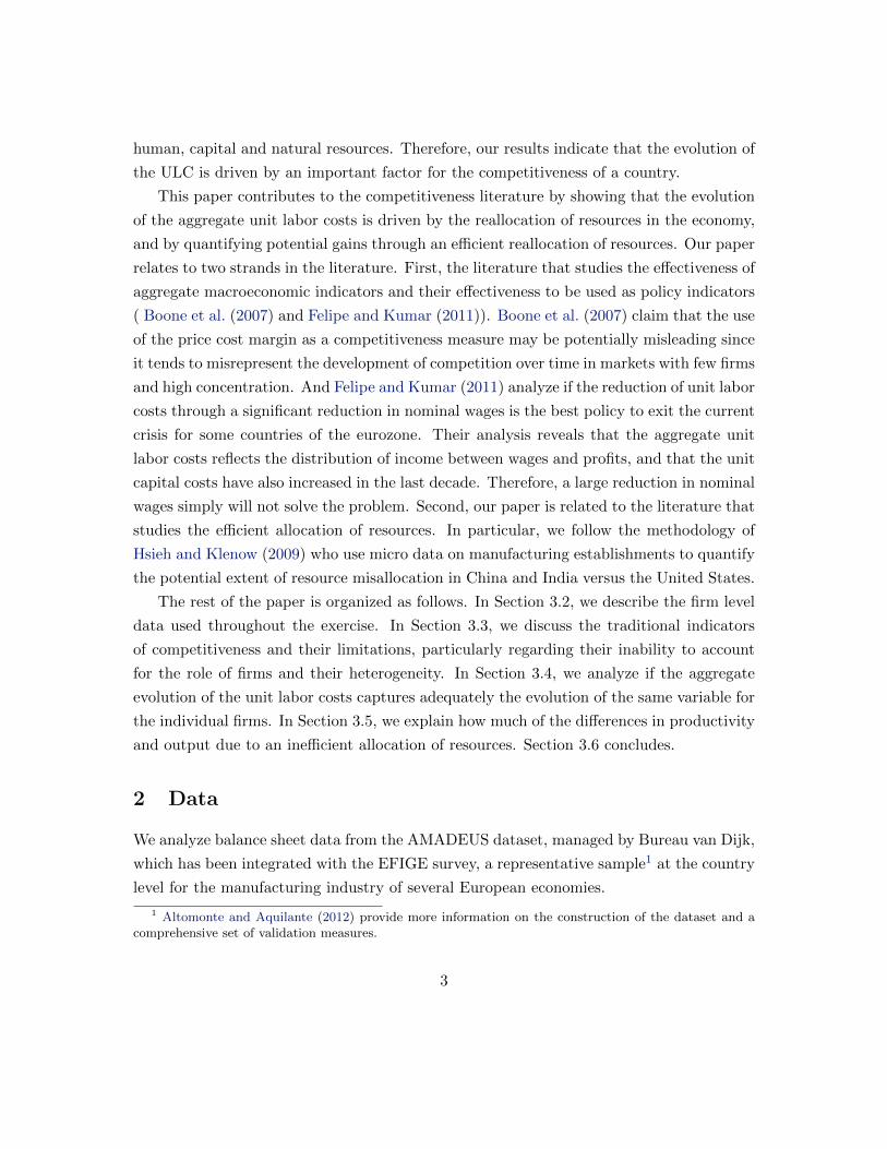
The analysis is centered on France, Germany, Italy and Spain.2 While for the analysis

of the ULC only the cost of employees and the turnover of the firm are needed, the study

of the impact of an efficient reallocation of resources requires data both from the balance

sheet and the survey which we specify in detail later.

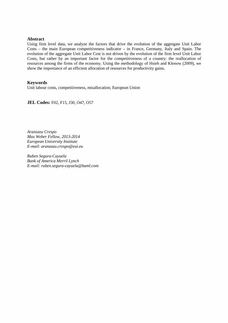
For each surveyed firm, nine years of usable balance sheet information has been re-

trieved, from 2001 to 2009. France, Italy and Spain are the countries with best quality in

the balance sheet data, with a coverage3 of 88.6%, 86.86% and 90.56% respectively. For

Germany, the coverage is irregular. For the period of 2004-2008, there is a fairly good

coverage of 70% to 80% of the firms, however for the years 2001-2003 and 2009 it drops to

levels between 30-45% on average.

0.1

.2.3

.4.5

2 4 6 8 10 ln (employees)

EFIGEAMADEUS

(a) France

0.1

.2.3

.4

2 4 6 8 10 ln (employees)

EFIGEAMADEUS

(b) Germany

0.2

.4.6

2 4 6 8 10 ln (employees)

EFIGEAMADEUS

(c) Italy

0.2

.4.6

2 4 6 8 10 ln (employees)

EFIGEAMADEUS

(d) Spain

Figure 1: Distribution of Plant Size

2In the EFIGE dataset there is also information about three more European countries: Austria, Hungaryand United Kingdom. Due to the poor quality of the balanced data for these countries, they have not beenincluded in the analysis.

3The reference variable for the coverage is the turnover of the firm.

4

In Figure 1, we present the distribution of firms by employment size for all the surveyed

firms in EFIGE and the sample covered by the AMADEUS database. For all the countries

with the exception of Germany, the firm size distribution of the subsection of firms present

in AMADEUS matches almost perfectly the firm size distribution of the surveyed firms in

EFIGE. Within the subsection of firms present in the AMADEUS dataset for Germany,

the number of small firms is slightly under-represented while the number of medium firms

is slightly over-represented with respect to the distribution of all the surveyed firms in

EFIGE. Hence, we should be cautious in the interpretation of results for Germany and

make sure is that they are not biased by this fact.

3 Limitations of the Traditional Competitiveness Indicators

Porter (1990) defines the competitiveness of a nation as the productivity with which a

nation utilizes its human, capital and natural resources. The OECD considers the ability

of a country to sell its products in the international markets while Krugman (1994) refers

to competitiveness as a poetic way of speaking about productivity, and warns about the

danger of obsessing about the competitiveness of a country. Most of these definitions of

competitiveness allude to the relative position of a country in international trade. This

position, in principle, depends on price and cost factors because if they have a negative

evolution in relation with those from others economies, the ability to sell products at

home and abroad is damaged. This argument, combined with the easy availability of

data, makes price-cost competitiveness indicators especially attractive for the analysis of

a country’s economic situation. This is why the classical macroeconomic textbooks relate

the competitiveness of nations to the comparison of their relative prices.

Currently the price-cost indicator of reference to measure competitiveness in the Euro-

pean Union is the unit labor cost (ULC), which measures the labor cost by unit of product

and is calculated as the ratio of total labor costs to real output.4 A rise in an economy’s

ULC represents an increased reward for labor’s contribution to output. However, a rise in

labor costs higher than the rise in labor productivity may be a threat to an economy’s cost

competitiveness, if other costs are not adjusted in compensation.

A simple comparison of the evolution of prices and costs between two countries may

4An assumption implicit in the use of cost based indicators is that in the short run the capital is fixed,and therefore the cost of capital should not differ between similar countries. This assumption can be alimitation of the cost-competitiveness measures, see Felipe and Kumar (2011) for further details.

5

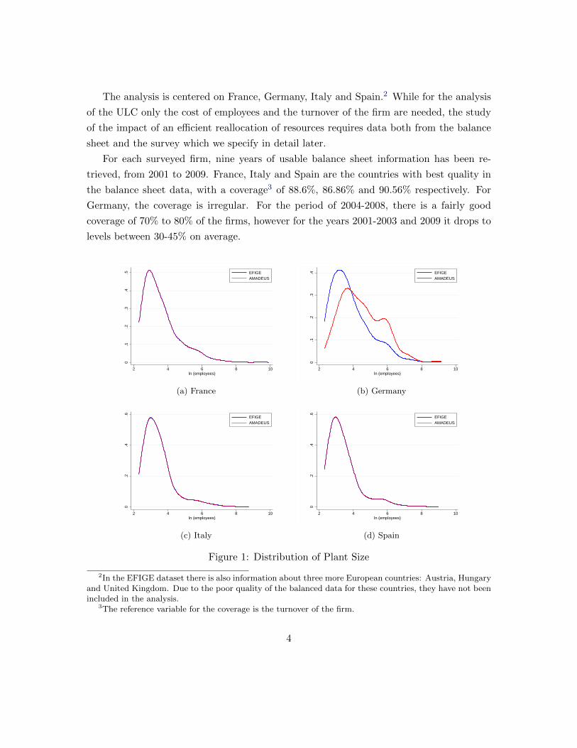
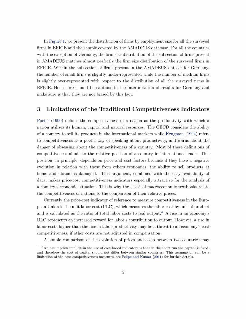
not be informative enough to determine the competitiveness of a country, and therefore,

the ULC may be a measure of competitiveness with a very limited prediction power. If

an increase in the ULC index indicates a loss in competitiveness of the country, then

we should see a decrease in a country’s export shares whenever aggregate ULC goes up.

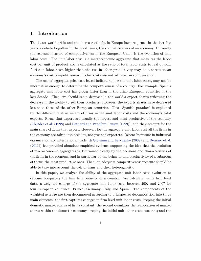
Figure 2 shows the so called Spanish competitiveness paradox, an example that a loss in

competitiveness does not imply necessarily a loss in the world’s export shares. Figure 2a

shows the evolution of the ULC for Spain and the main developed economies, while in

Figure 2b shows the evolution of these countries worlds’ export share during the 2000’s.

The Spanish ULC has grown faster than in the main developed countries, but on the other

hand, its export shares have decreased less than those of other countries, the only exception

being Germany.

BANCO DE ESPAÑA 106 ECONOMIC BULLETIN, JANUARY 2012 COMPETITIVENESS INDICATORS: THE IMPORTANCE OF AN EFFICIENT ALLOCATION OF RESOURCES

ciency of the imports of the country in question. Some authors (e.g. Krugman (1994)) criticise

the emphasis on international market shares as competitiveness indicators, insofar as they

give an overly mercantilist view and cannot say anything about the competitiveness of the na-

tion as a whole, but only of its exports.

One option followed in the literature consists in modifying the aggregated sectoral price/

cost measures so that they better capture non-price elements of competitiveness. A prom-

ising example of this approach, albeit still incapable of capturing all the relevant factors, is

the one that appears in Bennett et al. (2009). These authors argue that non-price elements

of competitiveness should be reflected in the elasticity of substitution of each product. Ac-

cordingly, they construct real exchange rates which allow such elasticity to differ from prod-

uct to product.

Finally, it should also be pointed out that there are a number of indicators that attempt to

measure the institutional characteristics of each country that may influence competitiveness.

This is the case, for example, of the Davos World Economic Forum’s Global Competitive-

ness Report and of the World Bank’s Doing Business Report. In general, these indicators

are constructed by conducting surveys of various experts of each country on the ease of

doing business in their country, which are sometimes supplemented with macroeconomic

indicators. This is a very valuable alternative that provides useful information, since it enables

areas to be identified in which some countries are clearly lagging. That said, the information

is subjective, there is sometimes a lack of robust empirical links between the variables ana-

lysed and competitiveness, and it is impossible to draw quantitative conclusions to guide

economic policy.

Given this wide range of alternative measures of competitiveness and the limitations of each,

it is not surprising that, for the purposes of the alert mechanism in the context of macroeco-

nomic surveillance and the excessive imbalances procedure recently launched at the Euro-

pean level, it has been decided to monitor the developments in a broad set of competitiveness

measures. These measures include the current account balance, ULCs, export shares and

CPI-deflated real exchange rates.

0.85

0.90

0.95

1.00

1.05

1.10

1.15

1.20

00 01 02 03 04 05 06 07 08 09 10

GERMANY SPAIN FRANCE

UNITED KINGDOM ITALY

1 COMPETITIVENESS INDICATORS VIS-À-VIS THE EURO AREA (a)

60

70

80

90

100

110

120

00 01 02 03 04 05 06 07 08 09 10

FRANCE GERMANY ITALY

SPAIN UNITED KINGDOM

2 MARKET SHARE INDEX (b)

COMPETITIVENESS CHART 1

SOURCES: ECB and WTO.

a An increase in the index implies a loss of competitiveness.b An increase in the index implies a gain of market share.

(a) Unit Labor Cost (ECB)

BANCO DE ESPAÑA 106 ECONOMIC BULLETIN, JANUARY 2012 COMPETITIVENESS INDICATORS: THE IMPORTANCE OF AN EFFICIENT ALLOCATION OF RESOURCES

ciency of the imports of the country in question. Some authors (e.g. Krugman (1994)) criticise

the emphasis on international market shares as competitiveness indicators, insofar as they

give an overly mercantilist view and cannot say anything about the competitiveness of the na-

tion as a whole, but only of its exports.

One option followed in the literature consists in modifying the aggregated sectoral price/

cost measures so that they better capture non-price elements of competitiveness. A prom-

ising example of this approach, albeit still incapable of capturing all the relevant factors, is

the one that appears in Bennett et al. (2009). These authors argue that non-price elements

of competitiveness should be reflected in the elasticity of substitution of each product. Ac-

cordingly, they construct real exchange rates which allow such elasticity to differ from prod-

uct to product.

Finally, it should also be pointed out that there are a number of indicators that attempt to

measure the institutional characteristics of each country that may influence competitiveness.

This is the case, for example, of the Davos World Economic Forum’s Global Competitive-

ness Report and of the World Bank’s Doing Business Report. In general, these indicators

are constructed by conducting surveys of various experts of each country on the ease of

doing business in their country, which are sometimes supplemented with macroeconomic

indicators. This is a very valuable alternative that provides useful information, since it enables

areas to be identified in which some countries are clearly lagging. That said, the information

is subjective, there is sometimes a lack of robust empirical links between the variables ana-

lysed and competitiveness, and it is impossible to draw quantitative conclusions to guide

economic policy.

Given this wide range of alternative measures of competitiveness and the limitations of each,

it is not surprising that, for the purposes of the alert mechanism in the context of macroeco-

nomic surveillance and the excessive imbalances procedure recently launched at the Euro-

pean level, it has been decided to monitor the developments in a broad set of competitiveness

measures. These measures include the current account balance, ULCs, export shares and

CPI-deflated real exchange rates.

0.85

0.90

0.95

1.00

1.05

1.10

1.15

1.20

00 01 02 03 04 05 06 07 08 09 10

GERMANY SPAIN FRANCE

UNITED KINGDOM ITALY

1 COMPETITIVENESS INDICATORS VIS-À-VIS THE EURO AREA (a)

60

70

80

90

100

110

120

00 01 02 03 04 05 06 07 08 09 10

FRANCE GERMANY ITALY

SPAIN UNITED KINGDOM

2 MARKET SHARE INDEX (b)

COMPETITIVENESS CHART 1

SOURCES: ECB and WTO.

a An increase in the index implies a loss of competitiveness.b An increase in the index implies a gain of market share.

(b) Market Share Index (WTO)

Figure 2: Competitiveness Indicators Vis-a-Vis the Euro Area

Antras et al. (2010) show that large Spanish firms experienced both lower ULC growth

and higher export growth than other countries, yet this differential is not reflected in

aggregate price indicators due to aggregation and dispersion bias (Altomonte et al. (2012)).

In the calculation of the ULC all the firms are taken into account while to calculate the

economy’s total exports, only the exporters are taken into account. Firms that export are

usually the largest and most productive of the economy (Clerides et al. (1998) and Bernard

and Bradford Jensen (1999)). The different relative weight in the aggregate ULC and in

the economy’s total export, helps therefore to explain the Spanish paradox.

An adequate competitiveness measure should be able to capture the role of firms and

their heterogeneity. Several questions arise then. First, why is heterogeneity so impor-

tant? Second, why should a competitiveness measure take into account the heterogeneity

within the firms of an economy? And third, how adequately do traditional competitiveness

6

measures capture the heterogeneity?

To understand the importance of the heterogeneity between firms, the concept of pro-

ductivity is essential since it allows high wages and high capital returns in an economy

(See Porter (2005)). Recent literature in industrial organization and international trade

has provided abundant empirical evidence supporting the idea that the evolution of macroe-

conomic aggregates is determined closely by the decisions and characteristics of the firms

in the economy, and in particular by the behavior and productivity of a subgroup of them:

the most productive ones. This is evident in the case of exporting firms. Exporter firms

from a sector or a country are a minority and, in general, they are those that behave better

in terms of productivity, size and innovation. The higher performance is present before

these firms become exporters (see Clerides et al. (1998) and Bernard et al. (2011)).

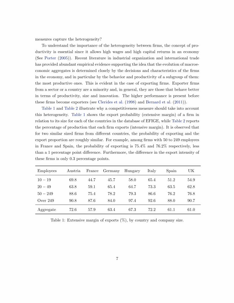
Table 1 and Table 2 illustrate why a competitiveness measure should take into account

this heterogeneity. Table 1 shows the export probability (extensive margin) of a firm in

relation to its size for each of the countries in the database of EFIGE, while Table 2 reports

the percentage of production that each firm exports (intensive margin). It is observed that

for two similar sized firms from different countries, the probability of exporting and the

export proportion are roughly similar. For example, among firms with 50 to 249 employees

in France and Spain, the probability of exporting is 75.4% and 76.2% respectively, less

than a 1 percentage point difference. Furthermore, the difference in the export intensity of

these firms is only 0.3 percentage points.

Employees Austria France Germany Hungary Italy Spain UK

10− 19 69.8 44.7 45.7 58.0 65.4 51.2 54.9

20− 49 63.8 59.1 65.4 64.7 73.3 63.5 62.8

50− 249 88.6 75.4 78.2 79.3 86.6 76.2 76.8

Over 249 90.8 87.6 84.0 97.4 92.6 88.0 90.7

Aggregate 72.6 57.9 63.4 67.3 72.2 61.1 61.0

Table 1: Extensive margin of exports (%), by country and company size.

7

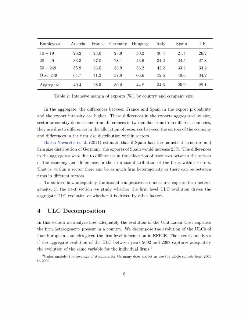
Employees Austria France Germany Hungary Italy Spain UK

10− 19 26.2 23.0 25.9 30.2 30.4 21.4 26.2

20− 49 33.3 27.0 28.1 43.6 34.2 24.5 27.8

50− 249 55.9 33.0 33.9 53.2 42.2 33.3 33.2

Over 249 64.7 41.2 37.8 66.6 52.6 40.6 34.2

Aggregate 40.4 28.5 30.0 44.8 34.6 25.9 29.1

Table 2: Intensive margin of exports (%), by country and company size.

In the aggregate, the differences between France and Spain in the export probability

and the export intensity are higher. These differences in the exports aggregated by size,

sector or country do not come from differences in two similar firms from different countries,

they are due to differences in the allocation of resources between the sectors of the economy

and differences in the firm size distribution within sectors.

Barba-Navaretti et al. (2011) estimate that if Spain had the industrial structure and

firm size distribution of Germany, the exports of Spain would increase 25%. The differences

in the aggregates were due to differences in the allocation of resources between the sectors

of the economy and differences in the firm size distribution of the firms within sectors.

That is, within a sector there can be as much firm heterogeneity as there can be between

firms in different sectors.

To address how adequately traditional competitiveness measures capture firm hetero-

geneity, in the next section we study whether the firm level ULC evolution drives the

aggregate ULC evolution or whether it is driven by other factors.

4 ULC Decomposition

In this section we analyze how adequately the evolution of the Unit Labor Cost captures

the firm heterogeneity present in a country. We decompose the evolution of the ULCs of

four European countries given the firm level information in EFIGE. The exercise analyzes

if the aggregate evolution of the ULC between years 2002 and 2007 captures adequately

the evolution of the same variable for the individual firms.5

5Unfortunately, the coverage of Amadeus for Germany does not let us use the whole sample from 2001to 2009.

8

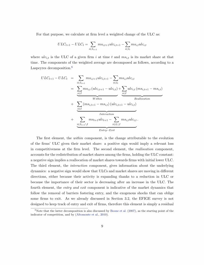
For that purpose, we calculate at firm level a weighted change of the ULC as:

ULCt+1 − ULCt =∑i∈It+1

msi,t+1ulci,t+1 −∑i∈It

msi,tulci,t

where ulci,t is the ULC of a given firm i at time t and msi,t is its market share at that

time. The components of the weighted average are decomposed as follows, according to a

Laspeyres decomposition.6

ULCt+1 − ULCt =∑i∈It+1

msi,t+1ulci,t+1 −∑i∈It

msi,tulci,t

=∑i∈I

msi,t (ulci,t+1 − ulci,t)︸ ︷︷ ︸Within

+∑i∈I

ulci,t (msi,t+1 −msi,t)︸ ︷︷ ︸Reallocation

+∑i∈I

(msi,t+1 −msi,t) (ulci,t+1 − ulci,t)︸ ︷︷ ︸Interaction

+∑

i∈It+1\I

mst+1ulct+1 −∑i∈It\I

msi,tulci,t︸ ︷︷ ︸Entry−Exit

.

The first element, the within component, is the change attributable to the evolution

of the firms’ ULC given their market share: a positive sign would imply a relevant loss

in competitiveness at the firm level. The second element, the reallocation component,

accounts for the redistribution of market shares among the firms, holding the ULC constant:

a negative sign implies a reallocation of market shares towards firms with initial lower ULC.

The third element, the interaction component, gives information about the underlying

dynamics: a negative sign would show that ULCs and market shares are moving in different

directions, either because their activity is expanding thanks to a reduction in ULC or

because the importance of their sector is decreasing after an increase in the ULC. The

fourth element, the entry and exit component is indicative of the market dynamics that

follow the removal of barriers fostering entry, and the exogenous shocks that can oblige

some firms to exit. As we already discussed in Section 3.2, the EFIGE survey is not

designed to keep track of entry and exit of firms, therefore this element is simply a residual

6Note that the latter decomposition is also discussed by Boone et al. (2007), as the starting point of theindicator of competition, and by (Altomonte et al., 2010).

9

of the calculation, and will be ignored in the discussion.

If the aggregate ULC was a measure that captured adequately the heterogeneity existent

at the firm level ULC, its evolution should be driven by the evolution of the firm level ULC.

Then we should observe the within component to be the most relevant in the explanation

of the aggregate ULC evolution.

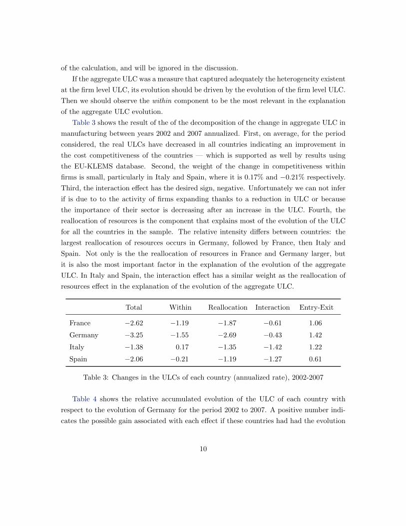
Table 3 shows the result of the of the decomposition of the change in aggregate ULC in

manufacturing between years 2002 and 2007 annualized. First, on average, for the period

considered, the real ULCs have decreased in all countries indicating an improvement in

the cost competitiveness of the countries — which is supported as well by results using

the EU-KLEMS database. Second, the weight of the change in competitiveness within

firms is small, particularly in Italy and Spain, where it is 0.17% and −0.21% respectively.

Third, the interaction effect has the desired sign, negative. Unfortunately we can not infer

if is due to to the activity of firms expanding thanks to a reduction in ULC or because

the importance of their sector is decreasing after an increase in the ULC. Fourth, the

reallocation of resources is the component that explains most of the evolution of the ULC

for all the countries in the sample. The relative intensity differs between countries: the

largest reallocation of resources occurs in Germany, followed by France, then Italy and

Spain. Not only is the the reallocation of resources in France and Germany larger, but

it is also the most important factor in the explanation of the evolution of the aggregate

ULC. In Italy and Spain, the interaction effect has a similar weight as the reallocation of

resources effect in the explanation of the evolution of the aggregate ULC.

Total Within Reallocation Interaction Entry-Exit

France −2.62 −1.19 −1.87 −0.61 1.06

Germany −3.25 −1.55 −2.69 −0.43 1.42

Italy −1.38 0.17 −1.35 −1.42 1.22

Spain −2.06 −0.21 −1.19 −1.27 0.61

Table 3: Changes in the ULCs of each country (annualized rate), 2002-2007

Table 4 shows the relative accumulated evolution of the ULC of each country with

respect to the evolution of Germany for the period 2002 to 2007. A positive number indi-

cates the possible gain associated with each effect if these countries had had the evolution

10

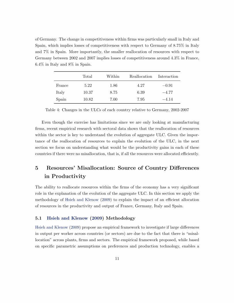
of Germany. The change in competitiveness within firms was particularly small in Italy and

Spain, which implies losses of competitiveness with respect to Germany of 8.75% in Italy

and 7% in Spain. More importantly, the smaller reallocation of resources with respect to

Germany between 2002 and 2007 implies losses of competitiveness around 4.3% in France,

6.4% in Italy and 8% in Spain.

Total Within Reallocation Interaction

France 5.22 1.86 4.27 −0.91

Italy 10.37 8.75 6.39 −4.77

Spain 10.82 7.00 7.95 −4.14

Table 4: Changes in the ULCs of each country relative to Germany, 2002-2007

Even though the exercise has limitations since we are only looking at manufacturing

firms, recent empirical research with sectoral data shows that the reallocation of resources

within the sector is key to understand the evolution of aggregate ULC. Given the impor-

tance of the reallocation of resources to explain the evolution of the ULC, in the next

section we focus on understanding what would be the productivity gains in each of these

countries if there were no misallocation, that is, if all the resources were allocated efficiently.

5 Resources’ Misallocation: Source of Country Differences

in Productivity

The ability to reallocate resources within the firms of the economy has a very significant

role in the explanation of the evolution of the aggregate ULC. In this section we apply the

methodology of Hsieh and Klenow (2009) to explain the impact of an efficient allocation

of resources in the productivity and output of France, Germany, Italy and Spain.

5.1 Hsieh and Klenow (2009) Methodology

Hsieh and Klenow (2009) propose an empirical framework to investigate if large differences

in output per worker across countries (or sectors) are due to the fact that there is “misal-

location” across plants, firms and sectors. The empirical framework proposed, while based

on specific parametric assumptions on preferences and production technology, enables a

11

clean representation of the potential impact of “misallocation” on sectoral or aggregate

productivity.

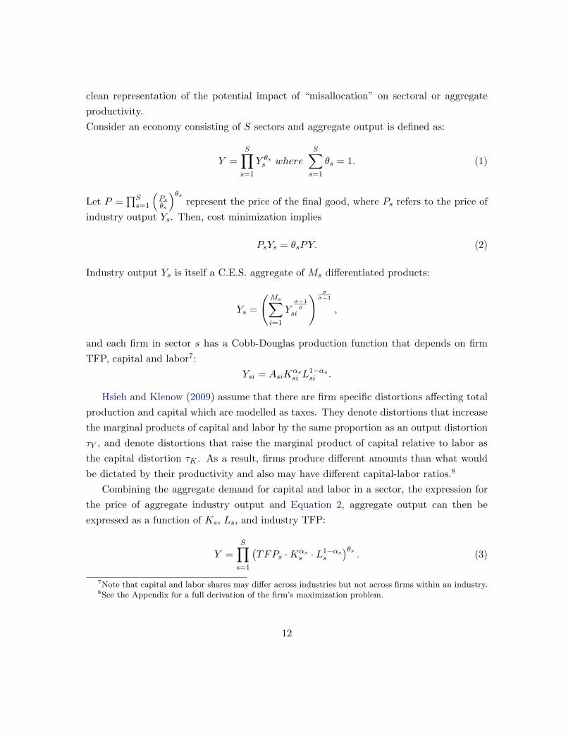
Consider an economy consisting of S sectors and aggregate output is defined as:

Y =S∏s=1

Y θss where

S∑s=1

θs = 1. (1)

Let P =∏Ss=1

(Psθs

)θsrepresent the price of the final good, where Ps refers to the price of

industry output Ys. Then, cost minimization implies

PsYs = θsPY. (2)

Industry output Ys is itself a C.E.S. aggregate of Ms differentiated products:

Ys =

(Ms∑i=1

Yσ−1σ

si

) σσ−1

,

and each firm in sector s has a Cobb-Douglas production function that depends on firm

TFP, capital and labor7:

Ysi = AsiKαssi L

1−αssi .

Hsieh and Klenow (2009) assume that there are firm specific distortions affecting total

production and capital which are modelled as taxes. They denote distortions that increase

the marginal products of capital and labor by the same proportion as an output distortion

τY , and denote distortions that raise the marginal product of capital relative to labor as

the capital distortion τK . As a result, firms produce different amounts than what would

be dictated by their productivity and also may have different capital-labor ratios.8

Combining the aggregate demand for capital and labor in a sector, the expression for

the price of aggregate industry output and Equation 2, aggregate output can then be

expressed as a function of Ks, Ls, and industry TFP:

Y =S∏s=1

(TFPs ·Kαs

s · L1−αss

)θs. (3)

7Note that capital and labor shares may differ across industries but not across firms within an industry.8See the Appendix for a full derivation of the firm’s maximization problem.

12

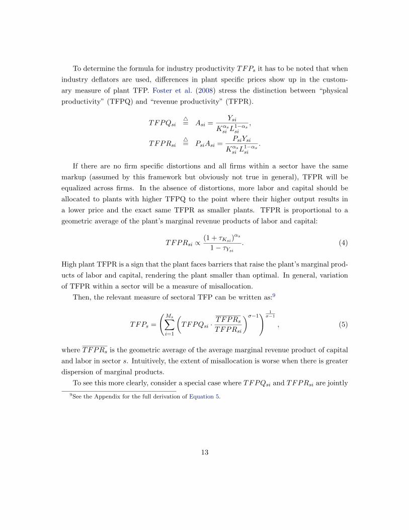
To determine the formula for industry productivity TFPs it has to be noted that when

industry deflators are used, differences in plant specific prices show up in the custom-

ary measure of plant TFP. Foster et al. (2008) stress the distinction between “physical

productivity” (TFPQ) and “revenue productivity” (TFPR).

TFPQsi4= Asi =

Ysi

Kαssi L

1−αssi

,

TFPRsi4= PsiAsi =

PsiYsi

Kαssi L

1−αssi

.

If there are no firm specific distortions and all firms within a sector have the same

markup (assumed by this framework but obviously not true in general), TFPR will be

equalized across firms. In the absence of distortions, more labor and capital should be

allocated to plants with higher TFPQ to the point where their higher output results in

a lower price and the exact same TFPR as smaller plants. TFPR is proportional to a

geometric average of the plant’s marginal revenue products of labor and capital:

TFPRsi ∝(1 + τKsi)

αs

1− τYsi. (4)

High plant TFPR is a sign that the plant faces barriers that raise the plant’s marginal prod-

ucts of labor and capital, rendering the plant smaller than optimal. In general, variation

of TFPR within a sector will be a measure of misallocation.

Then, the relevant measure of sectoral TFP can be written as:9

TFPs =

(Ms∑i=1

(TFPQsi ·

TFPRsTFPRsi

)σ−1) 1σ−1

, (5)

where TFPRs is the geometric average of the average marginal revenue product of capital

and labor in sector s. Intuitively, the extent of misallocation is worse when there is greater

dispersion of marginal products.

To see this more clearly, consider a special case where TFPQsi and TFPRsi are jointly

9See the Appendix for the full derivation of Equation 5.

13

lognormally distributed, then the expression in Equation 5 implies:

logTFPs =1

σ − 1log

(Ms∑i=1

Aσ−1si

)− σ

2var(logTFPRsi),

so that the negative effect of distortions can be summarized by the variance of log TFPR.

5.2 Gains of an Efficient Allocation of Resources in Europe

In order to determine the gains from an efficient allocation of resources, we calculate

“efficient” output in each country so we can compare it with actual output levels. If there

are no firm specific distortions, TFPR will be equalized across firms within a sector. Then,

industry TFP would be As =(∑Ms

i=1Aσ−1si

) 1σ−1

. For each industry, we calculate the ratio

of actual TFP (Equation 5) to this efficient level of TFP, and then aggregate this ratio

across sectors using the Cobb-Douglas aggregator (Equation 1):

Y

Yefficient=

S∏s=1

[Ms∑i=1

(Asi

As

TFPRsTFPRsi

)σ−1] θsσ−1

(6)

To calculate the effects of resource misallocation, we need to estimate key parameters

(industry output shares, industry capital shares, and the firm-specific distortions) from the

data.

The data for France, Germany, Italy and Spain are drawn from the joint EFIGE-

Amadeus dataset. We use are the plant’s industry (four-digit level), age (based on reported

birth year), wage payments, value-added, export revenues, and capital stock. For labor

input we use the plant’s wage bill10 rather than its employment to measure Lsi. As a later

robustness check, we measure Lsi as employment. We define capital stock as the book

value of fixed capital net of depreciation.

We set the rental price of capital (excluding distortions) to R = 0.10, we have in mind

a 5% real interest rate and a 5% depreciation rate.11 We set the elasticity of substitution

between plant value added to σ = 3, which ranges within the estimates of the substitutabil-

10The Amadeus data only report wage payments; the information on non-wage compensation is notreported.

11The actual cost of capital faced by plant i in industry s is denoted (1 + τKsi)R, so it differs from 10%if τKsi ≥ 0. Because our hypothetical reforms collapse τKsi to its average in each industry, if R is setincorrectly, it will affect the average capital distortion but not the experiment itself.

14

ity of competing manufactures in the trade and industrial organization literature (Broda

and Weinstein (2006)). Later, we entertain the higher value of 5 and a lower value of 2

for σ as a robustness check. We set the elasticity of output with respect to capital in each

industry (αs) to be 1 minus the labor share in the corresponding industry in Germany in

2008. We adopt the German shares as the benchmark.

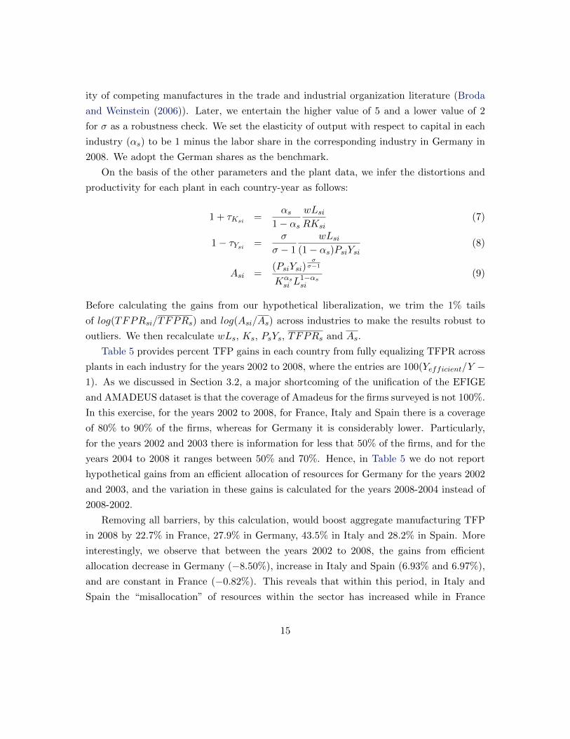
On the basis of the other parameters and the plant data, we infer the distortions and

productivity for each plant in each country-year as follows:

1 + τKsi =αs

1− αswLsiRKsi

(7)

1− τYsi =σ

σ − 1

wLsi(1− αs)PsiYsi

(8)

Asi =(PsiYsi)

σσ−1

Kαssi L

1−αssi

(9)

Before calculating the gains from our hypothetical liberalization, we trim the 1% tails

of log(TFPRsi/TFPRs) and log(Asi/As) across industries to make the results robust to

outliers. We then recalculate wLs, Ks, PsYs, TFPRs and As.

Table 5 provides percent TFP gains in each country from fully equalizing TFPR across

plants in each industry for the years 2002 to 2008, where the entries are 100(Yefficient/Y −1). As we discussed in Section 3.2, a major shortcoming of the unification of the EFIGE

and AMADEUS dataset is that the coverage of Amadeus for the firms surveyed is not 100%.

In this exercise, for the years 2002 to 2008, for France, Italy and Spain there is a coverage

of 80% to 90% of the firms, whereas for Germany it is considerably lower. Particularly,

for the years 2002 and 2003 there is information for less that 50% of the firms, and for the

years 2004 to 2008 it ranges between 50% and 70%. Hence, in Table 5 we do not report

hypothetical gains from an efficient allocation of resources for Germany for the years 2002

and 2003, and the variation in these gains is calculated for the years 2008-2004 instead of

2008-2002.

Removing all barriers, by this calculation, would boost aggregate manufacturing TFP

in 2008 by 22.7% in France, 27.9% in Germany, 43.5% in Italy and 28.2% in Spain. More

interestingly, we observe that between the years 2002 to 2008, the gains from efficient

allocation decrease in Germany (−8.50%), increase in Italy and Spain (6.93% and 6.97%),

and are constant in France (−0.82%). This reveals that within this period, in Italy and

Spain the “misallocation” of resources within the sector has increased while in France

15

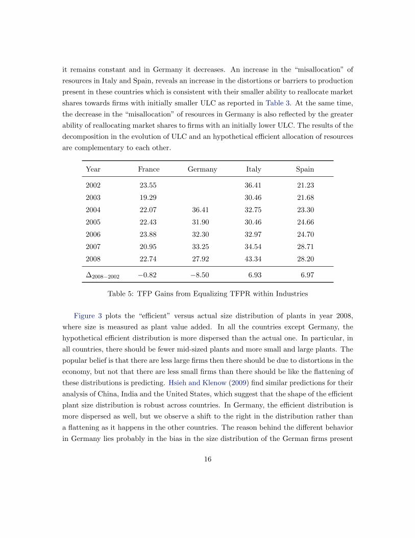
it remains constant and in Germany it decreases. An increase in the “misallocation” of

resources in Italy and Spain, reveals an increase in the distortions or barriers to production

present in these countries which is consistent with their smaller ability to reallocate market

shares towards firms with initially smaller ULC as reported in Table 3. At the same time,

the decrease in the “misallocation” of resources in Germany is also reflected by the greater

ability of reallocating market shares to firms with an initially lower ULC. The results of the

decomposition in the evolution of ULC and an hypothetical efficient allocation of resources

are complementary to each other.

Year France Germany Italy Spain

2002 23.55 36.41 21.23

2003 19.29 30.46 21.68

2004 22.07 36.41 32.75 23.30

2005 22.43 31.90 30.46 24.66

2006 23.88 32.30 32.97 24.70

2007 20.95 33.25 34.54 28.71

2008 22.74 27.92 43.34 28.20

∆2008−2002 −0.82 −8.50 6.93 6.97

Table 5: TFP Gains from Equalizing TFPR within Industries

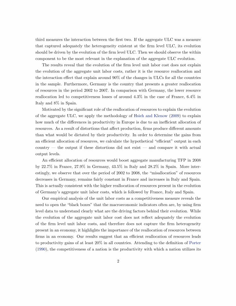
Figure 3 plots the “efficient” versus actual size distribution of plants in year 2008,

where size is measured as plant value added. In all the countries except Germany, the

hypothetical efficient distribution is more dispersed than the actual one. In particular, in

all countries, there should be fewer mid-sized plants and more small and large plants. The

popular belief is that there are less large firms then there should be due to distortions in the

economy, but not that there are less small firms than there should be like the flattening of

these distributions is predicting. Hsieh and Klenow (2009) find similar predictions for their

analysis of China, India and the United States, which suggest that the shape of the efficient

plant size distribution is robust across countries. In Germany, the efficient distribution is

more dispersed as well, but we observe a shift to the right in the distribution rather than

a flattening as it happens in the other countries. The reason behind the different behavior

in Germany lies probably in the bias in the size distribution of the German firms present

16

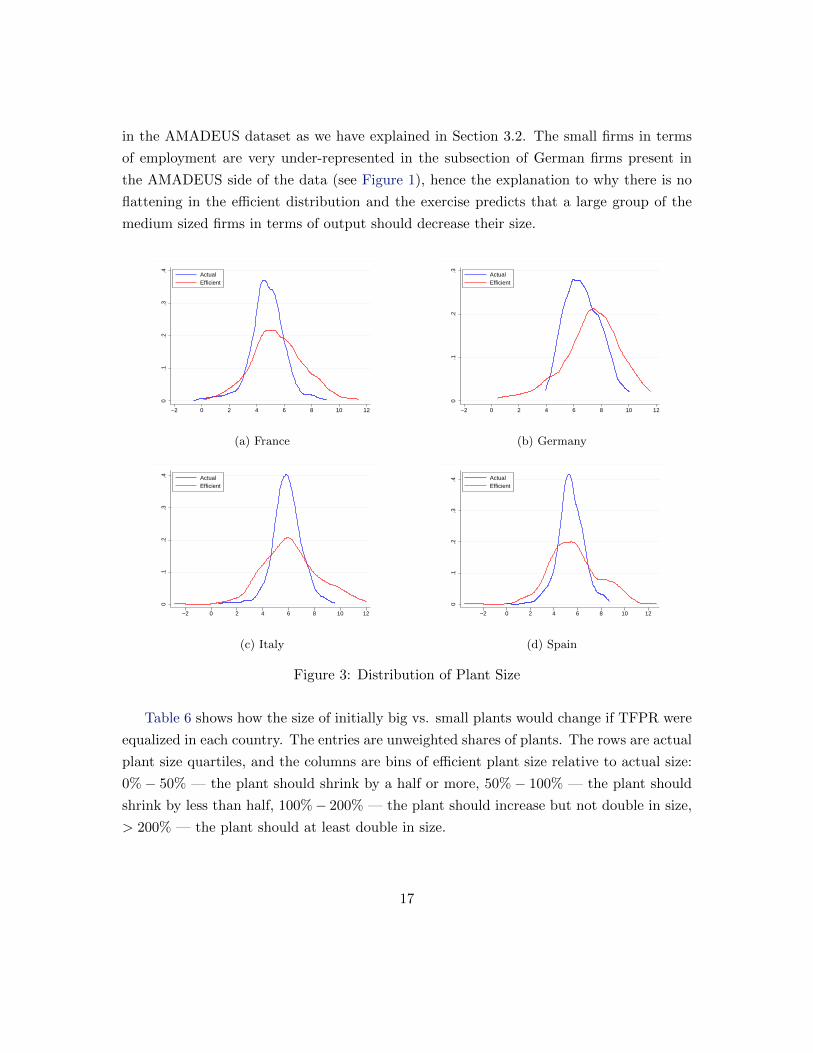
in the AMADEUS dataset as we have explained in Section 3.2. The small firms in terms

of employment are very under-represented in the subsection of German firms present in

the AMADEUS side of the data (see Figure 1), hence the explanation to why there is no

flattening in the efficient distribution and the exercise predicts that a large group of the

medium sized firms in terms of output should decrease their size.

0.1

.2.3

.4

−2 0 2 4 6 8 10 12

ActualEfficient

(a) France0

.1.2

.3

−2 0 2 4 6 8 10 12

ActualEfficient

(b) Germany

0.1

.2.3

.4

−2 0 2 4 6 8 10 12

ActualEfficient

(c) Italy

0.1

.2.3

.4

−2 0 2 4 6 8 10 12

ActualEfficient

(d) Spain

Figure 3: Distribution of Plant Size

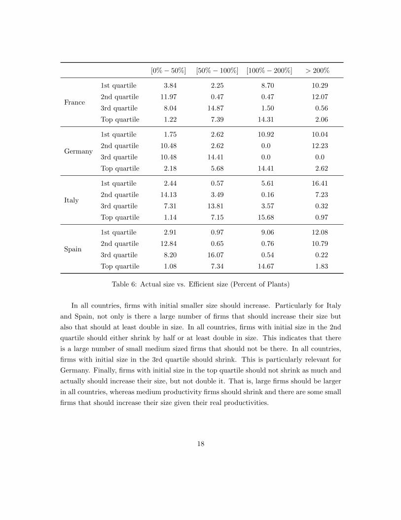
Table 6 shows how the size of initially big vs. small plants would change if TFPR were

equalized in each country. The entries are unweighted shares of plants. The rows are actual

plant size quartiles, and the columns are bins of efficient plant size relative to actual size:

0% − 50% — the plant should shrink by a half or more, 50% − 100% — the plant should

shrink by less than half, 100%− 200% — the plant should increase but not double in size,

> 200% — the plant should at least double in size.

17

[0%− 50%] [50%− 100%] [100%− 200%] > 200%

France

1st quartile 3.84 2.25 8.70 10.29

2nd quartile 11.97 0.47 0.47 12.07

3rd quartile 8.04 14.87 1.50 0.56

Top quartile 1.22 7.39 14.31 2.06

Germany

1st quartile 1.75 2.62 10.92 10.04

2nd quartile 10.48 2.62 0.0 12.23

3rd quartile 10.48 14.41 0.0 0.0

Top quartile 2.18 5.68 14.41 2.62

Italy

1st quartile 2.44 0.57 5.61 16.41

2nd quartile 14.13 3.49 0.16 7.23

3rd quartile 7.31 13.81 3.57 0.32

Top quartile 1.14 7.15 15.68 0.97

Spain

1st quartile 2.91 0.97 9.06 12.08

2nd quartile 12.84 0.65 0.76 10.79

3rd quartile 8.20 16.07 0.54 0.22

Top quartile 1.08 7.34 14.67 1.83

Table 6: Actual size vs. Efficient size (Percent of Plants)

In all countries, firms with initial smaller size should increase. Particularly for Italy

and Spain, not only is there a large number of firms that should increase their size but

also that should at least double in size. In all countries, firms with initial size in the 2nd

quartile should either shrink by half or at least double in size. This indicates that there

is a large number of small medium sized firms that should not be there. In all countries,

firms with initial size in the 3rd quartile should shrink. This is particularly relevant for

Germany. Finally, firms with initial size in the top quartile should not shrink as much and

actually should increase their size, but not double it. That is, large firms should be larger

in all countries, whereas medium productivity firms should shrink and there are some small

firms that should increase their size given their real productivities.

18

5.3 Robustness Tests

We now provide a number of robustness checks to our baseline Table 5 calculations of

hypothetical efficiency gains. We have measured plant labor input using its wage bill.

The logic is that wages per worker adjust for plant differences in hours worked per worker

and worker skills. However, wages could also reflect rent sharing between the plant and

its workers. If so, we might be interpreting differences in TFPR across plants because

the most profitable plants have to pay higher wages. We therefore recalculate the gains

from equalizing TFPR in France, Germany, Italy and Spain using simply employment as

our measure of plant labor input. The gains from an efficient allocation remain almost

unchanged for all countries with the exception of Germany — 21.18% for France, 35.44%

for Germany, 42.56% for Italy and 27.58% for Spain in 2008. The intuition behind the

smaller gains for Germany when we use the wage bill rather than the employees is that

wage differences may be limiting the TFPR differences.

We have assumed an elasticity of substitution within industries (σ) of 3. However the

literature on business cycles puts it at 2 while the literature more close to international

trade puts it at 5. Our estimates are sensitive to this parameter, with an increase between

10% and 20% in the gains from efficient allocation if σ = 5, and a decrease of 5% to 10% if

σ = 2. The intuition behind these results, is that when the elasticity of substitution within

industries is larger, then TFPR gaps are closed more slowly in response to reallocation of

inputs from low to high TFPR plants, enabling bigger gains from equalizing TFPR gains.

Given the dispersion in the size of the firms within the sectors and between countries,12

a last valid concern might be that the trimming of the productivity measures is large. Firms

with extreme productivity values have a high relative weight (following a trend more similar

to a Pareto distribution than a Normal distribution), which means that the behavior of the

sector aggregates are strongly influenced by the behavior of the largest firms (di Giovanni

and Levchenko (2009), Altomonte et al. (2010) and Altomonte et al. (2011)). Hence, less

trimming (or no trimming at all) in the right tail of the distribution, implies a higher

dispersion in the data observed, and we expect larger gains from an hypothetical efficient

allocation of resources. To analyze the robustness of the calculations to the dispersion in

firm size, we trim only 0.5% of the right tail of log(TFPRsi/TFPRs) before calculating

the hypothetical gains. While the results prove to be sensitive to this trimming, and as

12In Italy and Spain there is a smaller number of large firms than in Germany and France. See Crespo(2012) and Rubini et al. (2012).

19

expected there is an increase in the gains from an efficient allocation, this increase is similar

across countries (around 5%) — 26.86% in France, 33.97% in Germany, 49.33% in Italy and

35.46% in Spain. Between 2002 and 2008, the predicted gains from an efficient allocation

decrease in 3.64% in France, decrease in 9.20% in Germany, increase in 9.07% in Italy and

increase in 10.56%. While the variations are slightly larger, the ranking is unchanged and

therefore the conclusions of our exercise are consistent.

6 Conclusions

In this paper, we have analyzed the ability of the change in the aggregate unit labor cost

to capture the change in the competitiveness of a country.

Using firm level data, we calculate a weighted change of the aggregate unit labor costs

between 2002 and 2007 for four European countries: France, Germany, Italy and Spain.

The components of the weighted average are then decomposed according to a Laspeyres

decomposition into three main elements: the first captures changes in firm level unit labor

costs, keeping the initial domestic market shares of firms constant; the second quantifies

the reallocation of market shares within the domestic economy, keeping the initial unit

labor costs constant; and the third measures the interaction between the first two. The

results reveal that the evolution of the firm level unit labor cost does not explain the

evolution of the aggregate unit labor costs, rather it is the resource reallocation that drives

the evolution of the aggregate unit labor costs.

Motivated by the significant role of the reallocation of resources to explain the evolution

of the aggregate ULC, we apply the methodology of Hsieh and Klenow (2009) to analyze the

extent to which aggregate productivity differences between these four European countries

relate to inefficient resource reallocation. As a result of distortions that affect production,

firms produce different amounts than what would be dictated by their productivity. An

efficient allocation of resources would boost aggregate manufacturing TFP in 2008 by 22.7%

in France, 27.9% in Germany, 43.5% in Italy and 28.2% in Spain.

The empirical analysis of the unit labor costs as a competitiveness measure reveals the

need to use microeconomic data to understand the driving factors behind the evolution of

macroeconomic aggregates. And the decomposition of the aggregate indicator shows that

there are relevant differences among countries which in the aggregate cannot be observed

due to the noisiness of the measure.

20

References

Altomonte, C. and T. Aquilante (2012). The EU-EFIGE/Bruegel-Unicredit Dataset.

Bruegel Working Paper .

Altomonte, C., T. Aquilante, and G. Ottaviano (2012). The triggers of competitiveness:

The EFIGE cross-country report. Blueprint (17).

Altomonte, C., G. B. Navaretti, F. di Mauro, and G. Ottaviano (2011). Assessing compet-

itiveness: How firm-level data can help. Policy Contributions (643).

Altomonte, C., M. Nicolini, A. Rungi, and L. Ogliari (2010). Assessing the competitive

behaviour of firms in the single market: A micro-based approach. European Economy -

Economic Papers (409).

Antras, P., R. Segura-Cayuela, and D. Rodrıguez-Rodrıguez (2010). Firms in international

trade, with an application to spain. In SERIEs Invited Lecture at the XXXV Simposio

de la Asociacion Espanola de Economıa.

Barba-Navaretti, G., M. Bugamelli, F. Schivardi, C. Altomonte, D. Horgos, and D. Mag-

gioni (2011). The Global Operations of European Firms - The second EFIGE policy

report. Number 581 in Blueprints. Bruegel.

Bernard, A. B. and J. Bradford Jensen (1999). Exceptional exporter performance: cause,

effect, or both? Journal of International Economics 47 (1), 1–25.

Bernard, A. B., J. B. Jensen, S. J. Redding, and P. K. Schott (2011). The empirics of firm

heterogeneity and international trade. CEP Discussion Papers (dp1084).

Boone, J., H. van der Wiel, and J. C. van Ours (2007). How (not) to measure competition.

CEPR Discussion Papers (6275).

Broda, C. and D. E. Weinstein (2006). Globalization and the Gains from Variety. The

Quarterly Journal of Economics 121 (2), 541–585.

Clerides, S. K., S. Lach, and J. R. Tybout (1998). Is learning by exporting important?

micro-dynamic evidence from colombia, mexico, and morocco. The Quarterly Journal of

Economics 113 (3), 903–947.

21

Crespo, A. (2012). Trade, innovation and productivity: A quantitative analysis of Europe.

Working Paper EFIGE (62).

di Giovanni, J. and A. A. Levchenko (2009). International trade and aggregate fluctuations

in granular economies. Working Papers (585).

Felipe, J. and U. Kumar (2011). Unit labor costs in the eurozone: The competitiveness

debate again. Economics Working Paper Archive (651).

Foster, L., J. Haltiwanger, and C. Syverson (2008). Reallocation, firm turnover, and effi-

ciency: Selection on productivity or profitability? American Economic Review 98 (1),

394–425.

Hsieh, C.-T. and P. J. Klenow (2009). Misallocation and manufacturing tfp in china and

india. The Quarterly Journal of Economics 124 (4), 1403–1448.

Krugman, P. (1994). Competitiveness: A dangerous obsession. Technical report, Foreign

Affairs, vol 73(2).

Porter, M. (2005). What is competitiveness. Technical report, Notes on Globalization and

Strategy, IESE.

Porter, M. E. (1990). The Competitive Advantage of Nations. Free Press, New York.

Rubini, L., K. Desmet, F. Piguillem, and A. Crespo (2012). Breaking down the barriers

to firm growth in Europe: The fourth EFIGE policy report. Number 744 in Bruegel

Blueprints. Bruegel.

22

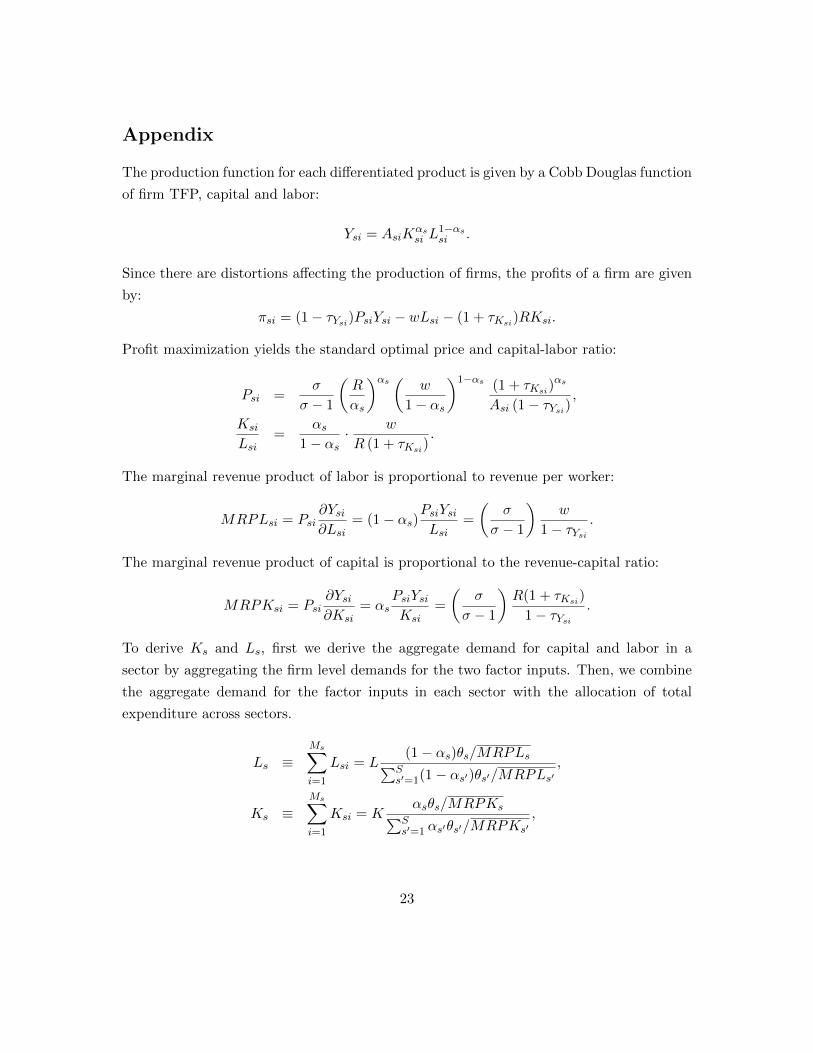
Appendix

The production function for each differentiated product is given by a Cobb Douglas function

of firm TFP, capital and labor:

Ysi = AsiKαssi L

1−αssi .

Since there are distortions affecting the production of firms, the profits of a firm are given

by:

πsi = (1− τYsi)PsiYsi − wLsi − (1 + τKsi)RKsi.

Profit maximization yields the standard optimal price and capital-labor ratio:

Psi =σ

σ − 1

(R

αs

)αs ( w

1− αs

)1−αs (1 + τKsi)αs

Asi (1− τYsi),

Ksi

Lsi=

αs1− αs

· w

R (1 + τKsi).

The marginal revenue product of labor is proportional to revenue per worker:

MRPLsi = Psi∂Ysi∂Lsi

= (1− αs)PsiYsiLsi

=

(σ

σ − 1

)w

1− τYsi.

The marginal revenue product of capital is proportional to the revenue-capital ratio:

MRPKsi = Psi∂Ysi∂Ksi

= αsPsiYsiKsi

=

(σ

σ − 1

)R(1 + τKsi)

1− τYsi.

To derive Ks and Ls, first we derive the aggregate demand for capital and labor in a

sector by aggregating the firm level demands for the two factor inputs. Then, we combine

the aggregate demand for the factor inputs in each sector with the allocation of total

expenditure across sectors.

Ls ≡Ms∑i=1

Lsi = L(1− αs)θs/MRPLs∑S

s′=1(1− αs′)θs′/MRPLs′,

Ks ≡Ms∑i=1

Ksi = Kαsθs/MRPKs∑S

s′=1 αs′θs′/MRPKs′,

23

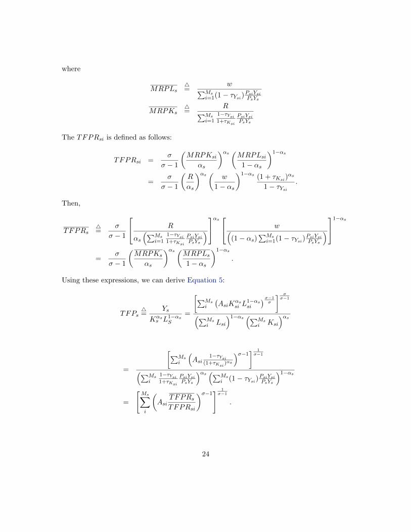
where

MRPLs4=

w∑Msi=1(1− τYsi)

PsiYsiPsYs

MRPKs4=

R∑Msi=1

1−τYsi1+τKsi

PsiYsiPsYs

The TFPRsi is defined as follows:

TFPRsi =σ

σ − 1

(MRPKsi

αs

)αs (MRPLsi1− αs

)1−αs

=σ

σ − 1

(R

αs

)αs ( w

1− αs

)1−αs (1 + τKsi)αs

1− τYsi.

Then,

TFPRs4=

σ

σ − 1

R

αs

(∑Msi=1

1−τYsi1+τKsi

PsiYsiPsYs

)αs w(

(1− αs)∑Ms

i=1(1− τYsi)PsiYsiPsYs

)1−αs

=σ

σ − 1

(MRPKs

αs

)αs (MRPLs1− αs

)1−αs.

Using these expressions, we can derive Equation 5:

TFPs4=

Ys

Kαss L1−αs

S

=

[∑Msi

(AsiK

αssi L

1−αssi

)σ−1σ

] σσ−1

(∑Msi Lsi

)1−αs (∑Msi Ksi

)αs

=

[∑Msi

(Asi

1−τYsi(1+τKsi )

αs

)σ−1] 1σ−1

(∑Msi

1−τYsi1+τKsi

PsiYsiPsYs

)αs (∑Msi (1− τYsi)

PsiYsiPsYs

)1−αs=

[Ms∑i

(Asi

TFPRsTFPRsi

)σ−1] 1σ−1

.

24