1  

Supporting Information for

The 16 April 2016, Mw 7.8 (MS 7.5) Ecuador earthquake: a quasi-repeat of

the 1942 MS 7.5 earthquake and partial re-rupture of the 1906 MS 8.6

Colombia-Ecuador earthquake

Lingling Yea,*, Hiroo Kanamoria, Jean-Philippe Avouaca, Linyan Lib, Kwok Fai Cheungb, Thorne Layc

aSeismological Laboratory, California Institute of Technology, Pasadena, CA 91125, USA

bDepartment of Ocean and Resources Engineering, University of Hawaii at Manoa, Honolulu, HI, 96822, USA

cDepartment of Earth and Planetary Sciences, University of California Santa Cruz, Santa Cruz, CA 95064, USA

*Corresponding author: Lingling Ye (lingling@gps.caltech.edu)

Contents of this file

Figures S1 to S9

Tables S1 to S3

Animations M1 to M4

Introduction

Supporting information includes 6 figures, 3 tables and 4 animations.

 

2  

 

   

Figure S1. (a) Map of the broadband seismic station distributions in North America (NA, diamonds) and Europe (EU, circles) for which high frequency teleseismic P waves are back-projected to the source region, as shown in Figures 2 and 5a. The station symbols are color-coded with the correlation coefficients for the first ~ 10 s of the aligned broadband P traces within each network. The red star shows the 2016 mainshock epicenter. (b) and (c) are aligned teleseismic P waves in the frequency band of 0.5 – 2 Hz for NA and EU networks, respectively.

 

3  

             

   

Figure S2. Megathrust geometry and source structure used in the finite-fault inversion for the 2016 Ecuador Earthquake. (a) Slab surface geometry approximated from slab 1.0 model [Hayes, 2012]. The red star shows the hypocenter of the 2016 event. (b) Source region velocity structure adapted from model Crust 2.0. Water depth varies with position for the offshore subfaults.

 

4  

 

Figure S3. Slip model with one additional up-dip row leading to tsunami mis-fit. (a) Slip distribution for the model with an additional up-dip row in the model relative to the final model (compare to Fig. 3) and outline of the initial rupture model (black). (b) Seafloor and land surface vertical displacement. (c) Near-field tsunami wave amplitude. The dash lines denote the trench and the shelf boundary defined at 200 m depth. (d) Tsunami wave peak amplitude across the eastern Pacific. (e) Comparison of recorded (black) and computed (red) waveforms at water-level stations. Note the early computed arrivals that result from even modest amounts of slip in the shallowest row compared to the final model in Figures 1, 3 and 4.

 

5  

 

Figure S4. Slip model shifted ~ 10 km inland. (a) Slip distribution for the model and outline of the initial rupture model (black). (b) Seafloor and land surface vertical displacement. (c) Near-field tsunami wave amplitude. The dash lines denote the trench and the shelf boundary defined at 200 m depth. (d) Tsunami wave peak amplitude across the eastern Pacific. (e) Comparison of recorded (black) and computed (red) waveforms at water-level stations. Note the late, smooth, and small computed arrivals at DART 32067 that result from even a modest down-dip shift of the rupture compared to the final model in Figures 1, 3 and 4.

 

6  

 

Figure S5. Comparison of observed (black lines) and computed (red lines) P-wave (a) and SH-wave (b) broadband ground displacement waveforms for the final slip model (Fig. 4).

 

7  

 

 

Figure S6. Predicted line-of-sight (LOS) displacements for InSAR ALOS-2 track140, Sentinel-1A ascending track 18 and descending track 40 from our best-fitting source model using the information about the LOS vectors provided by Xu and Sandwell (personal communication, 2016).    

 

8  

 

 

 

 

 

 

Figure S7. Foreshock and aftershock seismicity around the 2016 Ecuador Earthquake from the Geophysical Institute of the National Polytechnic School at Ecuador (http://www.igepn.edu.ec/portal/ultimo-­‐sismo/informe-­‐ultimo-­‐sismo.html). (a) Map view of seismicity from August 2015 to May 2016 around the 2016 Mw 7.8 Ecuador earthquake, color-coded with time difference from the Mw 7.8 mainshock and scaled with earthquake magnitude. (b) and (c) Plots of seismicity time sequence from the origin time and source latitude on a scale of months (b) and days (c).

 

9  

           

 

Figure S8. Companion of intensity produced by the 1942 (left) and 2016 (right) earthquakes. The intensity distribution for the 1942 earthquake is from Swenson and Beck [1996], and for the 2016 events it is from USGS/NEIC. The similarity of the intensity distributions suggests that the 1942 and 2016 events likely ruptured similar area on the megathrust.

 

10  

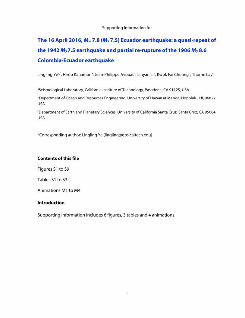
Figure S9. Comparison of N-S components of the 1906 and 2016 earthquakes. The black, red and green curves show the signals bandpass filtered in the frequency bands of 0.002 - 0.01 Hz, 0.002 - 0.0067 Hz and 0.002 - 0.005 Hz, respectively. The peak-to-peak amplitudes of all the band-passed records are normalized by the peak-to-peak amplitude. The similar dispersion between the two events supports our assumption that the signal for the 1906 event is the G1 Love wave.

 

11  

 Table S1. Comparison of 1906 and 1979 Tsunami Runup

Table S2. 1906, 1979 and 2016 Tsunami Runup

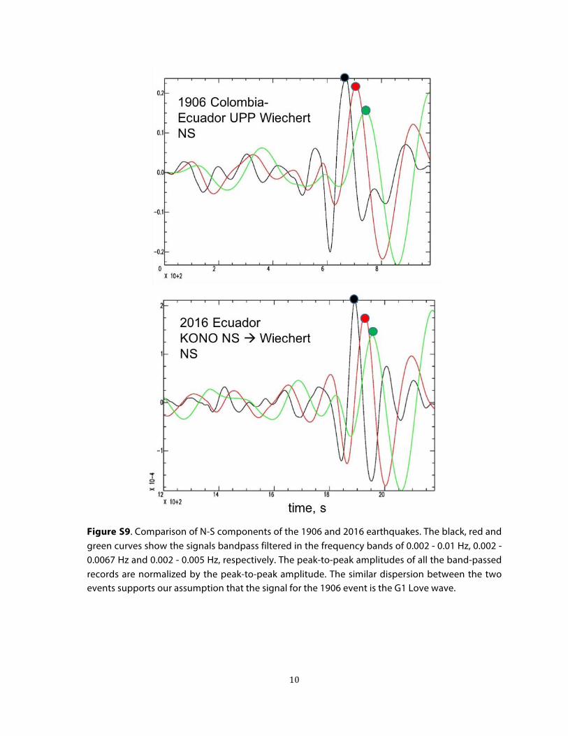
Table S2 continuous. 1979 Tsunami Runup

Country   Region   Lat   Lon   Distance   1906  (Mt)   1979  (Mt)  

COLOMBIA   GUAPI   2.57   -­‐77.88   438   1.00   2.00  COLOMBIA   TUMACO   1.83   -­‐78.73   321   5.00   3.00  JAPAN   HAKODATE   41.72   140.72   13654   0.17  (8.33)   0.10  (8.10)  JAPAN   AYUKAWA   38.30   141.50   13822   0.18  (8.36)   0.16  (8.30)  JAPAN   KUSHIMOTO   33.47   135.78   14553   0.24  (8.48)   0.09  (8.05)  US/HI   HILO   19.73   -­‐155.06   8253   1.80  (8.76)   0.40  (8.10)  US/HI   HONOLULU   21.31   -­‐157.87   8558   0.25  (8.70)   0.16  (8.50)  US/HI   KAHULUI   20.90   -­‐156.48   8411   0.30   0.34  

Travel  Time  Country   Region   Lat   Lon   Dist.  

Hours   Min  Max  

Height  

Mt  (Abe,  1979)  

1906-­‐01-­‐31  Columbia  (1.0°,  -­‐81.5°),  Mt_average  =  8.4  COLOMBIA   GUAPI   2.57   -­‐77.88   438   0   42   1.00    COLOMBIA   TUMACO   1.83   -­‐78.73   321   0   30   5.00    JAPAN   HAKODATE   41.72   140.72   13654   19   24   0.17   8.33  JAPAN   AYUKAWA   38.30   141.50   13822   19   48   0.18   8.36  JAPAN   HOSOSHIMA   32.43   131.67   14925   20   18   0.15   8.28  JAPAN   FUKAHORI   32.68   129.82   15037       0.28   8.55  JAPAN   NAGASAKI   32.73   129.87   15030   21   33   0.14   8.25  JAPAN   KUSHIMOTO   33.47   135.78   14553   20   27   0.24   8.48  

New  Zealand   GISBORNE   -­‐38.68   178.02   10988   26   25   0.60    PANAMA   NAOS_Is   8.92   -­‐79.53   907       0.70    US/CA   SAN_Diego   32.72   -­‐117.17   5133       0.05   8.00  US/CA   SAN_Francisco   37.81   -­‐122.47   5852       0.06   8.08  US/HI   HILO   19.73   -­‐155.06   8253   12   30   1.80   8.76  US/HI   HONOLULU   21.31   -­‐157.87   8558   11   42   0.25   8.70  US/HI   KAHULUI   20.90   -­‐156.48   8411       0.30    

2016-­‐01-­‐31  Ecuador  (0.35°,  -­‐79.93°)  ECUADOR   D32067   0.64   -­‐81.26   372   0   5      ECUADOR   Santa  Cruz  Is.   -­‐0.75   -­‐90.31   1255   3   2      ECUADOR   LA  LIBERTAD   -­‐2.23   -­‐80.90   669          

Country   Region   Lat   Lon   Dist.   Max  Height   Mt  (Abe,  1979)  

1979-­‐12-­‐12  Columbia     (1.0°,  -­‐79.5°),  Mt_average  =  8.1  COLOMBIA   BUENAVENTURA   3.89   -­‐77.07   360   0.14    COLOMBIA   EL_BARRO   2.60   -­‐77.70   215   1.00    COLOMBIA   EL_CHARCO   2.71   -­‐77.66   225   2.00    

 

12  

 

COLOMBIA   GUAPI   2.60   -­‐77.90   197   2.00    COLOMBIA   ISCUANDE   2.44   -­‐77.97   181   2.00    COLOMBIA   ISKA  GORGONA   3.00   -­‐78.32   194   5.00    COLOMBIA   LIMONES   2.61   -­‐77.80   207   2.00    COLOMBIA   SAN  JUAN  LA   2.33   -­‐78.60   117   6.00    COLOMBIA   TIMBIQUI   2.76   -­‐77.63   232   1.00    COLOMBIA   TUMACO   1.83   -­‐78.73   74   3.00    COLOMBIA   VUELTA  LARGA   2.65   -­‐77.90   200   3.00    COSTA  RICA   PUNTARENAS   9.97   -­‐84.83   1110   0.13    FRENCH     PAPEETE  TAHITI   -­‐17.53   -­‐149.57   7973   0.16    JAPAN   HACHINOHE   40.53   141.53   13769   0.21   8.42  JAPAN   HACHINOHE   40.52   141.52   13771   0.11   8.14  JAPAN   MUTSUOGAWARA   40.93   141.40   13750   0.06   7.88  JAPAN   CHICHIJIMA  Is.   27.09   142.19   14547   0.19   8.38  JAPAN   MERA   34.92   139.83   14267   0.07   7.95  JAPAN   ONAHAMA   36.93   140.90   14056   0.15   8.28  JAPAN   HAKODATE   41.72   140.72   13739   0.10   8.10  JAPAN   HANASAKI   43.28   145.57   13319   0.12   8.18  JAPAN   KUSHIRO   42.98   144.37   13417   0.09   8.05  JAPAN   TOKACHIKO   42.30   143.33   13530   0.25   8.50  JAPAN   URAKAWA   42.17   142.77   13576   0.12   8.18  JAPAN   HITACHIKO   36.50   140.63   14104   0.13   8.21  JAPAN   KAMAISHI   39.27   141.88   13831   0.17   8.33  JAPAN   MIYAKO   39.65   141.98   13799   0.15   8.28  JAPAN   OFUNATO   39.02   141.75   13857   0.18   8.36  JAPAN   SHIMANOKOSHIGYOKO   39.90   141.93   13785   0.24   8.48  JAPAN   NAZE   28.38   129.50   15483   0.10   8.10  JAPAN   MUROTOMISAKI   33.27   134.17   14788   0.05   7.80  JAPAN   TOSA-­‐SHIMIZU   32.78   132.96   14909   0.10   8.10  JAPAN   OWASE   34.08   136.20   14586   0.11   8.14  JAPAN   OWASE   34.08   136.20   14586   0.12   8.18  JAPAN   TOBA   34.48   136.82   14514   0.12   8.18  JAPAN   AYUKAWA   38.30   141.50   13922   0.16   8.30  JAPAN   ENOSHIMA   38.40   141.60   13909   0.03   7.58  JAPAN   ABURATSU   31.58   131.42   15106   0.13   8.21  JAPAN   MINAMI-­‐IZU   34.62   138.88   14356   0.06   7.88  JAPAN   OMAEZAKI   34.61   138.22   14405   0.09   8.05  JAPAN   TOKYO   35.65   139.77   14223   0.05   7.80  JAPAN   YAENE  HACHIJO   33.10   139.77   14390   0.06   7.88  JAPAN   KUSHIMOTO   33.47   135.78   14659   0.09   8.05  JAPAN   URAGAMI   33.55   135.90   14645   0.11   8.14  MEXICO   MANZANILLO   19.05   -­‐104.33   3342   0.50    MEXICO   ACAPULCO   16.83   -­‐99.92   2816   0.30    US/HI   HILO   19.73   -­‐155.06   8454   0.40   8.10  US/HI   HONOLULU   21.31   -­‐157.87   8755   0.16   8.50  US/HI   KAHULUI   20.90   -­‐156.48   8609   0.34    US/HI   NAWILIWILI   21.93   -­‐159.36   8913   0.14    US/HI   JOHNSTON   16.74   -­‐169.53   9977   0.10    

 

13  

Table S3. Surface Wave Magnitude

Station   Sta_lat(°)   Sta_lon(°)   Dist  (°)   Az(°)   Amp  (μm)   Ms  

1906-­‐01-­‐31  Columbia  (1°,  -­‐81.5°),  Ms_average  =  8.6    Jena   50.93   11.60   91.2   39.2   4242+   8.69  Osaka   34.70   135.52   130.3   319.4   3000   8.8  

Mizusawa   39.13   141.13   124.1   320.5   1544*   8.47  Potsdam   52.38   13.07   92.0   37.7   5000   8.9  Leipzig   51.33   12.40   91.7   38.8   4000   8.8  Sitka   57.05   -­‐135.33   70.3   332.1   7000   8.9  

Vieques   18.15   -­‐65.44   23.3   41.9   10000   8.0  Cheltenham   38.73   -­‐76.85   37.9   5.9   2360+   7.83  Honolulu   21.30   -­‐157.82   76.9   291.5   6000   8.9  Christch   -­‐43.53   172.62   102.2   225.7   2000   8.7  Zikawei   31.20   121.43   141.2   327.8   4000   8.9  Bombay   18.90   72.82   147.9   50.6   2000   8.7  Tiflis   41.72   44.80   115.5   42.0   1000   8.4  

(Sources:  Gutenberg  notepad;  *  from  original  records;+  from  station  bulletin)  1942-­‐05-­‐14     Ecuador  (-­‐3/4°,  -­‐81.5°),  Ms_average  =  7.9  

HAI   36.13   -­‐117.98   50.4   319.7   2?   7.6  HAI   36.13   -­‐117.98   50.4   319.7   1000   8.2  RIV   -­‐33.83   51.17   123.2   131.5   400   7.9  

PERTH   -­‐31.95   15.83   94.9   121.9   1400   8.5  UPP   59.85   17.64   93.8   30.1   240(?)   7.6  C?           200   7.8  A?       130     3?   7.6  

(Source:  Gutenberg  notepad)  1958-­‐01-­‐19  Ecuador  (1.0°,  -­‐79.5°),  Ms_average  =  7.3  

PAS   34.15   -­‐118.17   49.0   316.6   100   6.9  Aberdeen   57.17   -­‐2.10   82.3   32.4   200   7.3  Bucarest   44.41   26.10   100.4   44.6   150   7.3  Berkley   37.93   -­‐122.25   53.8   318.3   330   7.3  KEW   51.47   -­‐0.32   82.5   38.3   200   7.3  

LaPlate   -­‐34.90   -­‐57.93   41.1   152.6   800   7.4  Praha   50.08   14.42   91.8   40.0   300   7.6  UPP   59.85   17.64   92.7   30.1   200   7.4  

Kirurna   67.85   20.22   92.7   22.0   300   7.6  (Source:  Gutenberg  notepad)  

 

14  

Table S3. Continuous

1979-­‐12-­‐12  Columbia     (1°,  -­‐79.5°),  Ms_average  =  7.7  ALQ       41.7   326   430   7.3  GOL       44.7   331   100   7.8  PAS       48.6   316   321   7.3  PAS       48.6   316   473   7.5  BKS       53.4   318   490   7.6  BKS       53.4   318   560   7.6  MSO       54.2   331   436   7.6  NEW       56.7   331   450   7.6  NEW       56.7   331   350   7.7  PMR       79.1   333   50   8.2  COL       79.5   336   52   6.9  DBN       85.4   38   680   8.0  STU       87.8   41   148   7.4  GRF       89.1   41   557   8.0  MOX       89.4   40   34   8.2  MOX       89.4   40   323   7.9  HFS       90.1   30   624   8.1  SPA       91.6   180   67   7.1  KRA       94.7   40   90   7.3  KRA       94.7   40   373   8.0  SPC       95.1   41   464   8.0  GRM       104.2   124   125   7.5  PRE       106.5   116   37   7.0  SSE       142.1   331   302   8.4  

(Source:  USGS/NEIC)  

 

15  

 Animations

M1 – Back-projections of 0.5-2.0 Hz P waves from NA and EU networks.

 

16  

M2 – Zoom-in tsunami animation to DART 32067 and along the coast of Ecuador.

M3 – Large-Area tsunami animation to 3 DART stations and along the coasts of South and Central America.

 

17  

M4 – Rupture animation for slip (top) and cumulative slip (bottom) for the preferred fault model for the 2016 Ecuador earthquake. The moment-rate function is shown above each slip distribution, with a moving time indicator.